Computing Science 1P Lecture 19: Friday 9 th March Simon Gay Department of Computing Science...
66
Computing Science 1P Lecture 19: Friday 9 th March Simon Gay Department of Computing Science University of Glasgow 2006/07
-
Upload
ellen-watts -
Category
Documents
-
view
214 -
download
1
Transcript of Computing Science 1P Lecture 19: Friday 9 th March Simon Gay Department of Computing Science...

Computing Science 1P
Lecture 19: Friday 9th March
Simon GayDepartment of Computing Science
University of Glasgow
2006/07

2006/07 Computing Science 1P Lecture 19 - Simon Gay 2
What's coming up?
Fri 9th March (today): lecture as normalMon 12th – Wed 14th March: labs: FPPWed 14th March: lecture / tutorial as normalFri 16th March: NO LECTURE
EASTER BREAK: Mon 19th March – Fri 6th April
Tue 10th – Wed 11th April: Monday is a holidayDrop-in labs / FPP
Wed 11th April: lecture / tutorial as normal
NORMAL SCHEDULE RESUMES

2006/07 Computing Science 1P Lecture 19 - Simon Gay 3
Free Programming Project 2
We feel that the FPP in semester 1 was very beneficial forthose of you who did it, and there is some evidence that youenjoyed it too.
So, there will be another FPP now, and the handout describesit.
As an added incentive, there will be prizes for the best projects.
2006/07 Computing Science 1P Lecture 19 - Simon Gay 4
FPP Timetable
Fri 9th March: Unit 16 (FPP2) handed out. Start thinkingabout what you want to do.
Mon 12th – Wed 14th March: Discuss your idea with your tutor; write a clear specification, work on a plan.
Easter Break: Further work on your project, if you wish.
Tue 10th – Wed 11th April: Further work and advice from tutors.
Mon 16th – Wed 18th April: Demonstration to your tutor; submission (there will also be another Unit this week)
Tutors will nominate the best projects from each group; the lecturers willselect the winners; winners will also be asked to explain their programs.
2006/07 Computing Science 1P Lecture 19 - Simon Gay 5
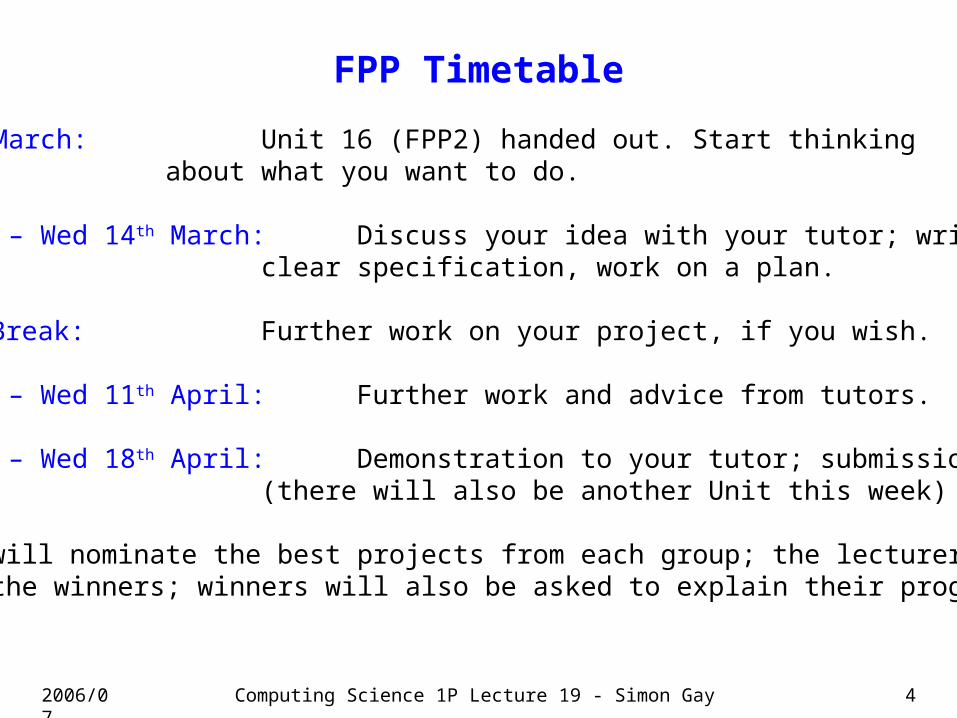
More on function parameters
We are very familiar with the idea of defining a function withparameters:
def test(x,y,z):
and then calling the function with the correct number ofparameters in the correct order:
f(1,"hello",1.2)
So far, this is the norm in most programming languages.Python is unusually flexible in providing extra features.
2006/07 Computing Science 1P Lecture 19 - Simon Gay 6
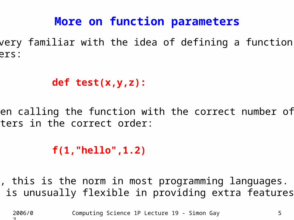
Naming the parameters when calling a function
Optionally we can give the name of the parameter when wecall the function:
f(x=1,y="hello",z=1.2)
Why would we do this?
If the parameters have informative names, then the functioncall (as well as the function definition) becomes more readable:
def lookup(phonebook,name):
number = lookup(phonebook = myBook, name = "John")

2006/07 Computing Science 1P Lecture 19 - Simon Gay 7
More on naming parameters
If we name the parameters when calling a function, then wedon't have to put them in the correct order:
number = lookup(phonebook = myBook, name = "John")
number = lookup(name = "John", phonebook = myBook)
are both correct.

2006/07 Computing Science 1P Lecture 19 - Simon Gay 8
Default values of parameters
We can specify a default value for a parameter of a function.Giving a value to that parameter when calling the function thenbecomes optional.
def lookup(phonebook,name,errorvalue="")
Example:
then number = lookup(myBook, "John")
is equivalent to
number = lookup(myBook, "John", "")
2006/07 Computing Science 1P Lecture 19 - Simon Gay 9
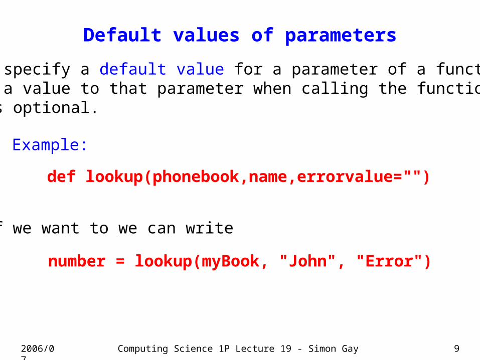
Default values of parameters
We can specify a default value for a parameter of a function.Giving a value to that parameter when calling the function thenbecomes optional.
def lookup(phonebook,name,errorvalue="")
Example:
number = lookup(myBook, "John", "Error")
If we want to we can write

2006/07 Computing Science 1P Lecture 19 - Simon Gay 10
Algorithms
We're going to spend a little time discussing algorithms,a central aspect of computing science and programming.
An algorithm is a systematic method or procedure for solving aproblem. Every computer program is based on one or morealgorithms: sometimes simple, sometimes very complex.

2006/07 Computing Science 1P Lecture 19 - Simon Gay 11
Quoted from Wikipedia:
The word algorithm comes from the name of the 9th century Persian mathematician Abu Abdullah Muhammad ibn Musa al-Khwarizmi whose works introduced Arabic numerals and algebraic concepts. He worked in Baghdad at the time when it was the centre of scientific studies and trade.
The word algorism originally referred only to the rules of performing arithmetic using Arabic numerals but evolved via European Latin translation of al-Khwarizmi's name into algorithm by the 18th century. The word evolved to include all definite procedures for solving problems or performing tasks.

2006/07 Computing Science 1P Lecture 19 - Simon Gay 12
Algorithms
For a given problem there may be several algorithms whichwill give the solution. We are often interested in the mostefficient algorithm; usually this means the fastest.
A fundamental discovery of computing science is theexistence of so-called NP-complete problems. These are problems which, as far as we know, cannot be solvedefficiently; however, an efficient algorithm for any one of themwould mean that we could solve all of them efficiently.
We'll say a little more about this later, but first let's see how different algorithms can be more or less efficient.
2006/07 Computing Science 1P Lecture 19 - Simon Gay 13
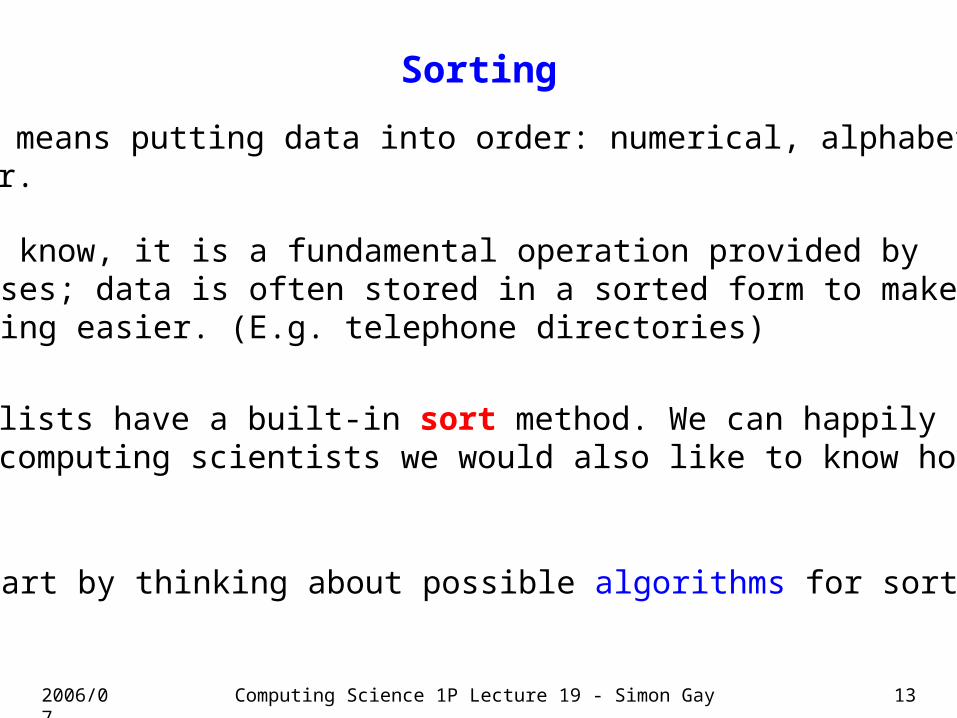
Sorting
Sorting means putting data into order: numerical, alphabetical,whatever.
As you know, it is a fundamental operation provided bydatabases; data is often stored in a sorted form to makesearching easier. (E.g. telephone directories)
Python lists have a built-in sort method. We can happily use it,but as computing scientists we would also like to know how itworks.
Let's start by thinking about possible algorithms for sorting.

2006/07 Computing Science 1P Lecture 19 - Simon Gay 14
How do we put things in order?
Think specifically about a list of numbers; we want to put theminto increasing order. How do we do it?
Obvious idea:
Find the smallest number (we know how to do that!).Remove it and put it into the first position of a new list.
Now find the smallest of the remaining numbers; it shouldbecome the second item of the new list.
And so on.

2006/07 Computing Science 1P Lecture 19 - Simon Gay 15
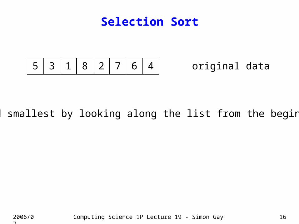
Selection Sort
5 3 1 8 2 7 6 4 original data
2006/07 Computing Science 1P Lecture 19 - Simon Gay 16
Selection Sort
5 3 1 8 2 7 6 4 original data
find smallest by looking along the list from the beginning

2006/07 Computing Science 1P Lecture 19 - Simon Gay 17
1
Selection Sort
5 3 8 2 7 6 4 original data
find smallest by looking along the list from the beginning

2006/07 Computing Science 1P Lecture 19 - Simon Gay 18
Selection Sort
5 3 8 2 7 6 4 original data
start a new list with the smallest item
1 sorted data

2006/07 Computing Science 1P Lecture 19 - Simon Gay 19
Selection Sort
5 3 8 2 7 6 4 original data
1 sorted data
find smallest by looking along the list from the beginning

2006/07 Computing Science 1P Lecture 19 - Simon Gay 20
Selection Sort
5 3 8 7 6 4 original data
1 sorted data
put the smallest item into the new list
2

2006/07 Computing Science 1P Lecture 19 - Simon Gay 21
Selection Sort
5 3 8 7 6 4 original data
1 sorted data
put the smallest item into the new list
2
and so on, until the original list is empty

2006/07 Computing Science 1P Lecture 19 - Simon Gay 22
Selection Sort: Alternative
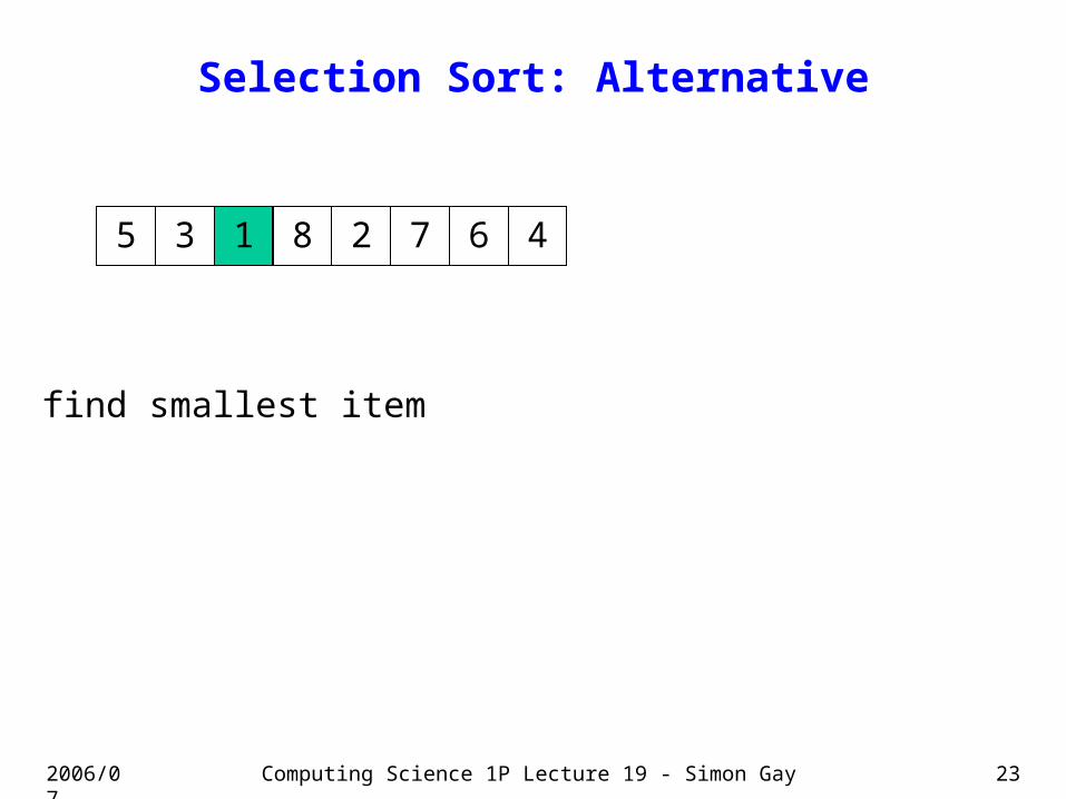
It is possible to reformulate the algorithm so that instead ofremoving items from the original list and putting them in a newlist, we modify the original list by moving items within it.
(In fact this is the more usual way to present it).
2006/07 Computing Science 1P Lecture 19 - Simon Gay 23
Selection Sort: Alternative
5 3 1 8 2 7 6 4
find smallest item

2006/07 Computing Science 1P Lecture 19 - Simon Gay 24
Selection Sort: Alternative
5 3 1 8 2 7 6 4
swap it with the first item

2006/07 Computing Science 1P Lecture 19 - Simon Gay 25
Selection Sort: Alternative
1 3 5 8 2 7 6 4
swap it with the first item
2006/07 Computing Science 1P Lecture 19 - Simon Gay 26
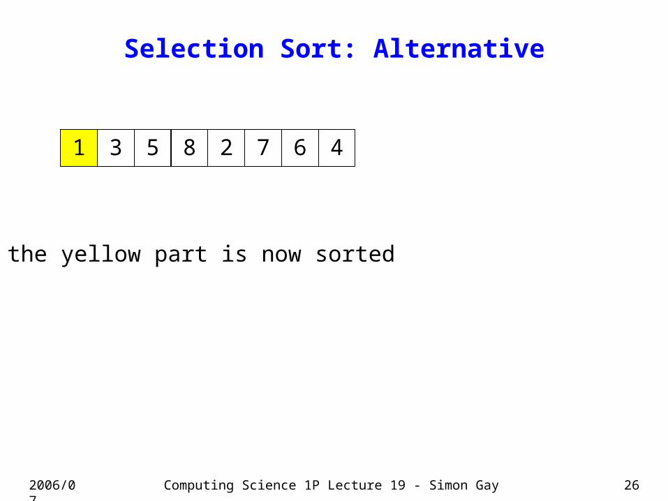
Selection Sort: Alternative
1 3 5 8 2 7 6 4
the yellow part is now sorted
2006/07 Computing Science 1P Lecture 19 - Simon Gay 27
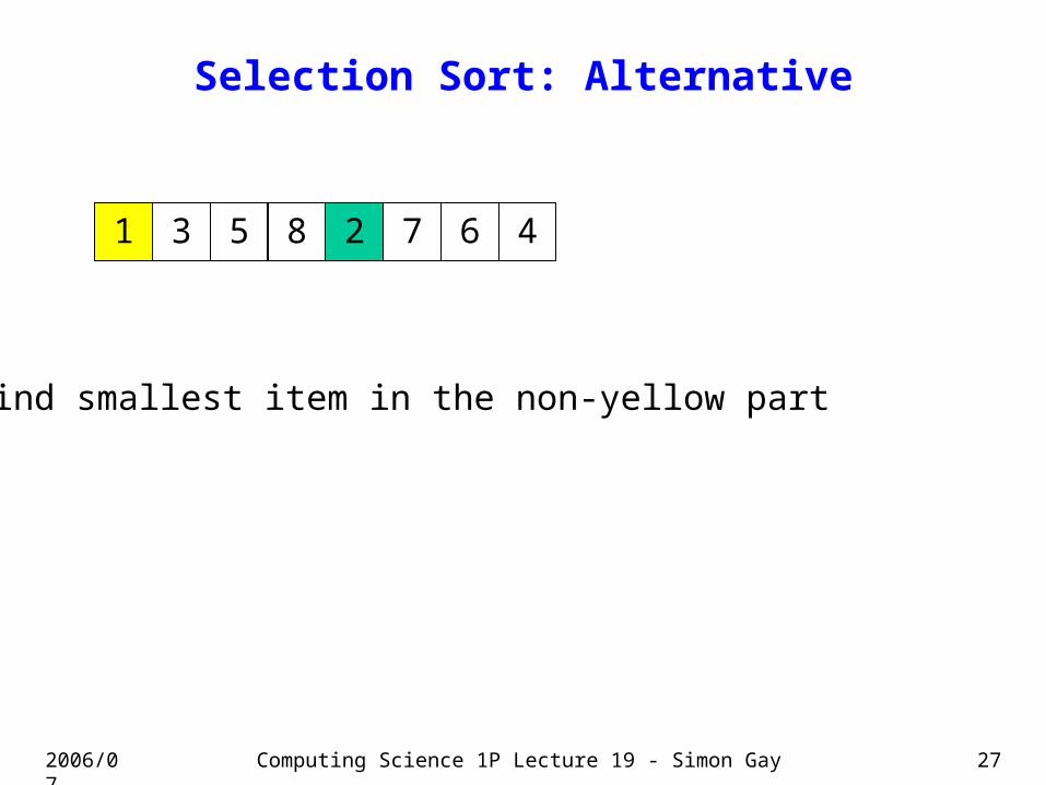
Selection Sort: Alternative
1 3 5 8 2 7 6 4
find smallest item in the non-yellow part

2006/07 Computing Science 1P Lecture 19 - Simon Gay 28
Selection Sort: Alternative
1 3 5 8 2 7 6 4
swap it with the first item in the non-yellow part

2006/07 Computing Science 1P Lecture 19 - Simon Gay 29
Selection Sort: Alternative
1 2 5 8 3 7 6 4
swap it with the first item in the non-yellow part
2006/07 Computing Science 1P Lecture 19 - Simon Gay 30
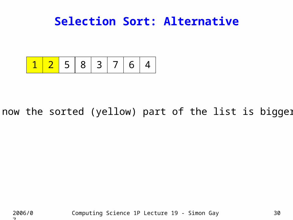
Selection Sort: Alternative
1 2 5 8 3 7 6 4
and now the sorted (yellow) part of the list is bigger

2006/07 Computing Science 1P Lecture 19 - Simon Gay 31
Selection Sort: Alternative
1 2 5 8 3 7 6 4
continue…

2006/07 Computing Science 1P Lecture 19 - Simon Gay 32
Selection Sort: Alternative
1 2 3 8 5 7 6 4
continue…

2006/07 Computing Science 1P Lecture 19 - Simon Gay 33
Selection Sort: Alternative
1 2 3 8 5 7 6 4
continue…
2006/07 Computing Science 1P Lecture 19 - Simon Gay 34
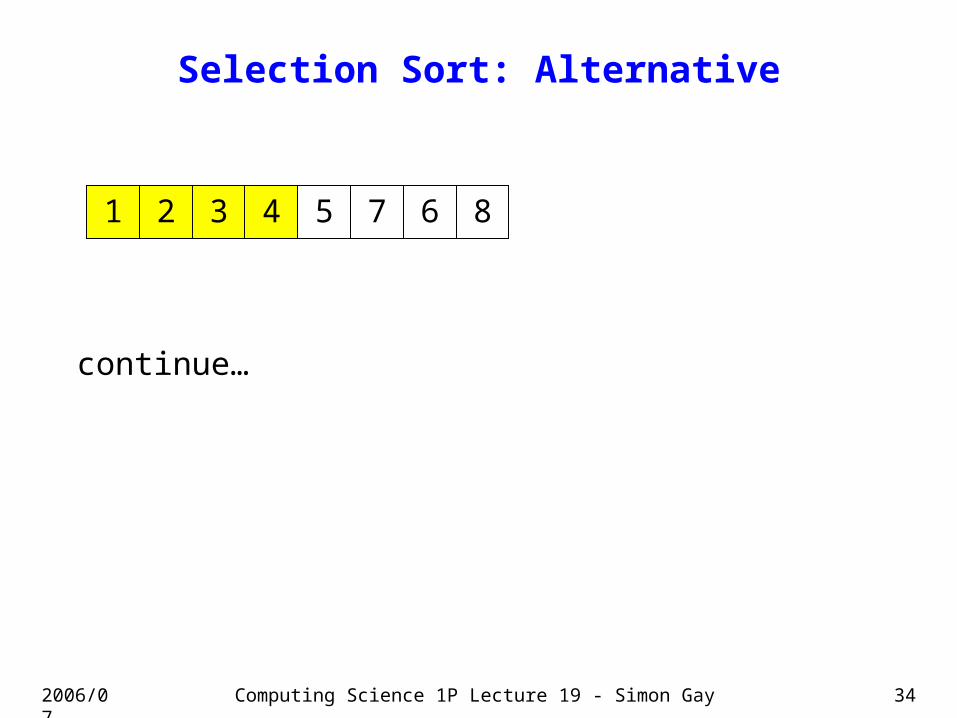
Selection Sort: Alternative
1 2 3 4 5 7 6 8
continue…

2006/07 Computing Science 1P Lecture 19 - Simon Gay 35
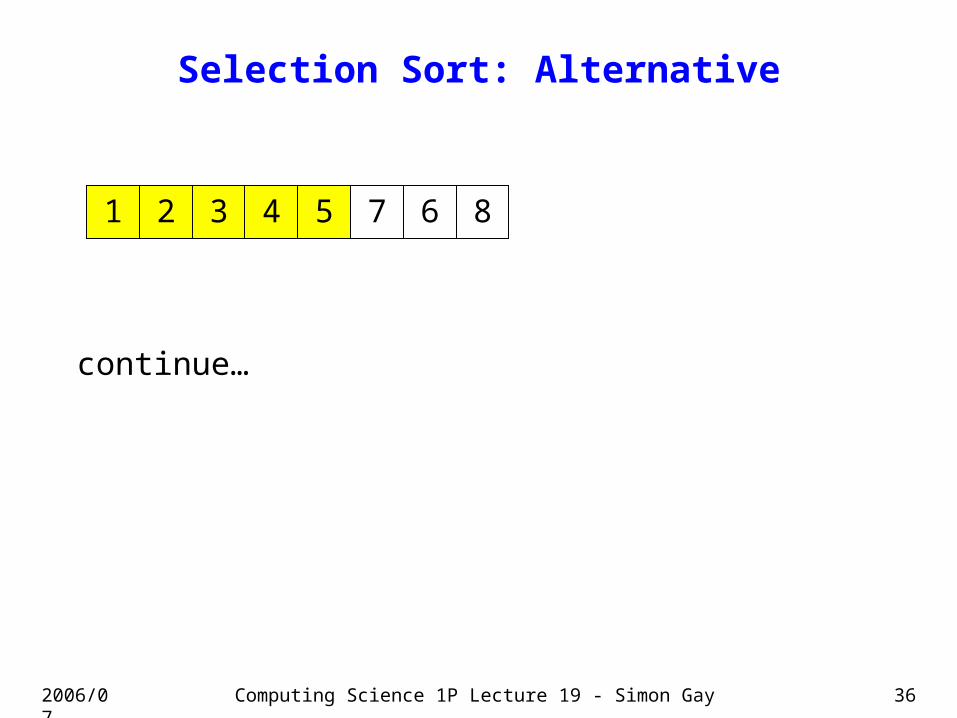
Selection Sort: Alternative
1 2 3 4 5 7 6 8
continue… 5 is in place already
2006/07 Computing Science 1P Lecture 19 - Simon Gay 36
Selection Sort: Alternative
1 2 3 4 5 7 6 8
continue…
2006/07 Computing Science 1P Lecture 19 - Simon Gay 37
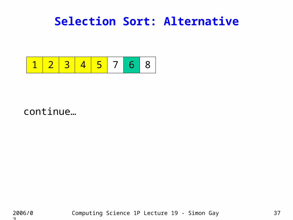
Selection Sort: Alternative
1 2 3 4 5 7 6 8
continue…
2006/07 Computing Science 1P Lecture 19 - Simon Gay 38
Selection Sort: Alternative
1 2 3 4 5 6 7 8
continue…

2006/07 Computing Science 1P Lecture 19 - Simon Gay 39
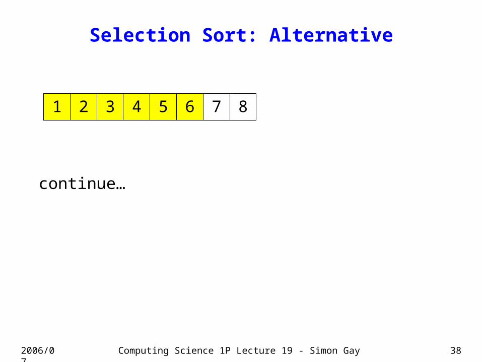
Selection Sort: Alternative
1 2 3 4 5 6 7 8
continue… 7 is in place already

2006/07 Computing Science 1P Lecture 19 - Simon Gay 40
Selection Sort: Alternative
1 2 3 4 5 6 7 8
continue… the last item is guaranteed to be in place

2006/07 Computing Science 1P Lecture 19 - Simon Gay 41
Selection Sort: Alternative
1 2 3 4 5 6 7 8
finished

2006/07 Computing Science 1P Lecture 19 - Simon Gay 42
Selection Sort in Python
The first version, which builds a new list:
def sort(x): s = [] while len(x) > 0: p = 0 # position of minimum so far i = 1 while i < len(x): # loop over the rest of x if x[i] < x[p]: # smaller item found p = i # update position i = i + 1 s = s + [x[p]] # put smallest in the new list del x[p] # and remove from x return s

2006/07 Computing Science 1P Lecture 19 - Simon Gay 43
Selection Sort in Python
The second version, which modifies the original list:
def sort(x): i = 0 while i < len(x): p = i # position of minimum so far j = i+1 while j < len(x): # loop over the rest of x if x[j] < x[p]: # smaller item found p = j # update position j = j + 1 temp = x[i] # move smallest into position i, x[i] = x[p] # extending the sorted region x[p] = temp # of x i = i + 1

2006/07 Computing Science 1P Lecture 19 - Simon Gay 44
Analyzing Selection Sort
How can we begin to analyze the efficiency (meaning speed)of selection sort?
Of course we could try it on various data sets and measure thetime taken, but because different computers have differentprocessing speeds in general, the time taken to sort 1000numbers on my computer does not tell you much about howlong it would take on your computer.
Also, as computing scientists, we would like to understandsomething more fundamental than empirical measurements.

2006/07 Computing Science 1P Lecture 19 - Simon Gay 45
Counting Comparisons
The first idea is to analyze the algorithm and work out howmany computational steps are needed to solve a problem of agiven size.
For sorting algorithms it turns out that the most relevant kindof computational step is the comparison of two items in the list.
If the items are large pieces of data, e.g. long strings, thencomparing them can be slow, and all of the other steps in thealgorithm are relatively quick.
For sorting algorithms we are interested in the number ofcomparisons needed to sort n items, expressed in terms of n.

2006/07 Computing Science 1P Lecture 19 - Simon Gay 46
Analyzing Selection Sort
Assume that we start with a list of length n.
To find the smallest item, we go round a loop n-1 times,doing a comparison each time (items 2 … n are each comparedwith the smallest item found so far).
Then we find the smallest of n-1 items, then the smallest of n-2,and so on.
The total number of comparisons is
(n-1) + (n-2) + (n-3) + … + 2 + 1

2006/07 Computing Science 1P Lecture 19 - Simon Gay 47
Analyzing Selection Sort
If you are taking Maths, you know that
(n-1) + (n-2) + (n-3) + … + 2 + 1 = n(n-1)/2
which can easily be proved by induction.
Or:
n
n-1

2006/07 Computing Science 1P Lecture 19 - Simon Gay 48
Analyzing Selection Sort
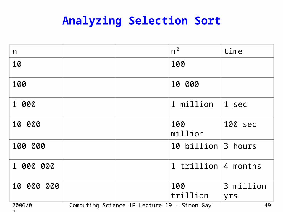
Selection sort needs n(n-1)/2 comparisons to sort n items.
As n becomes large, the dominant term is n²/2 and we say thatselection sort is an order n² algorithm.
This tells us something useful, independently of the speed of aparticular computer.
If it takes a certain time to sort a certain data set, then to sort10 times more data will take 100 times as long. To sort 1000times more data will take 1 000 000 times as long. And so on.
2006/07 Computing Science 1P Lecture 19 - Simon Gay 49
Analyzing Selection Sort
n n² time
10 100
100 10 000
1 000 1 million 1 sec
10 000 100 million 100 sec
100 000 10 billion 3 hours
1 000 000 1 trillion 4 months
10 000 000 100 trillion 3 million yrs
2006/07 Computing Science 1P Lecture 19 - Simon Gay 50
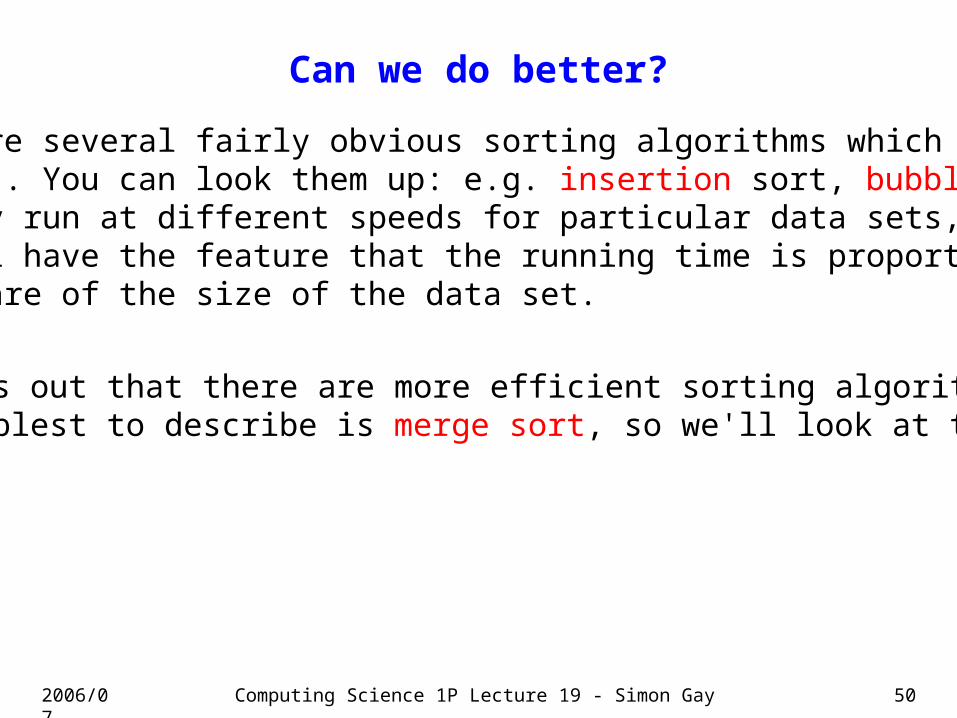
Can we do better?
There are several fairly obvious sorting algorithms which are allorder n². You can look them up: e.g. insertion sort, bubble sort.They may run at different speeds for particular data sets, butthey all have the feature that the running time is proportional tothe square of the size of the data set.
It turns out that there are more efficient sorting algorithms.The simplest to describe is merge sort, so we'll look at that.

2006/07 Computing Science 1P Lecture 19 - Simon Gay 51
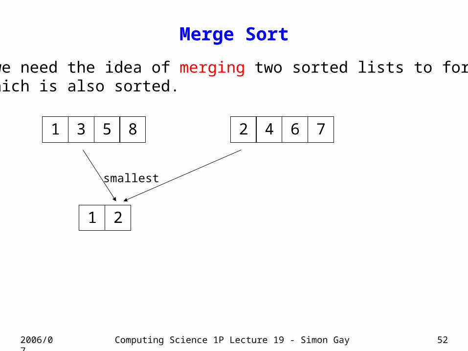
Merge Sort
First we need the idea of merging two sorted lists to form a newlist which is also sorted.
1 3 5 8 2 4 6 7
1
smallest
2006/07 Computing Science 1P Lecture 19 - Simon Gay 52
Merge Sort
First we need the idea of merging two sorted lists to form a newlist which is also sorted.
1 3 5 8 2 4 6 7
1
smallest
2

2006/07 Computing Science 1P Lecture 19 - Simon Gay 53
Merge Sort
First we need the idea of merging two sorted lists to form a newlist which is also sorted.
1 3 5 8 2 4 6 7
1
smallest
2 3

2006/07 Computing Science 1P Lecture 19 - Simon Gay 54
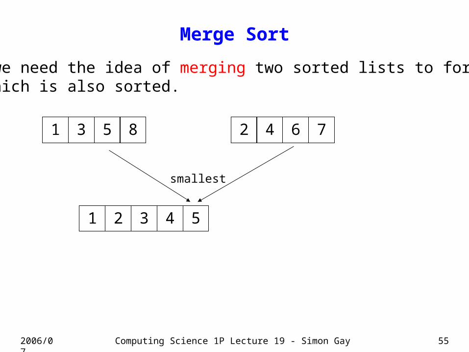
Merge Sort
First we need the idea of merging two sorted lists to form a newlist which is also sorted.
1 3 5 8 2 4 6 7
1
smallest
2 3 4
2006/07 Computing Science 1P Lecture 19 - Simon Gay 55
Merge Sort
First we need the idea of merging two sorted lists to form a newlist which is also sorted.
1 3 5 8 2 4 6 7
1
smallest
2 3 4 5

2006/07 Computing Science 1P Lecture 19 - Simon Gay 56
Merge Sort
First we need the idea of merging two sorted lists to form a newlist which is also sorted.
1 3 5 8 2 4 6 7
1
smallest
2 3 4 5 6

2006/07 Computing Science 1P Lecture 19 - Simon Gay 57
Merge Sort
First we need the idea of merging two sorted lists to form a newlist which is also sorted.
1 3 5 8 2 4 6 7
1
smallest
2 3 4 5 6 7

2006/07 Computing Science 1P Lecture 19 - Simon Gay 58
Merge Sort
First we need the idea of merging two sorted lists to form a newlist which is also sorted.
1 3 5 8 2 4 6 7
1
only thing left
2 3 4 5 6 7 8
2006/07 Computing Science 1P Lecture 19 - Simon Gay 59
Merge Sort
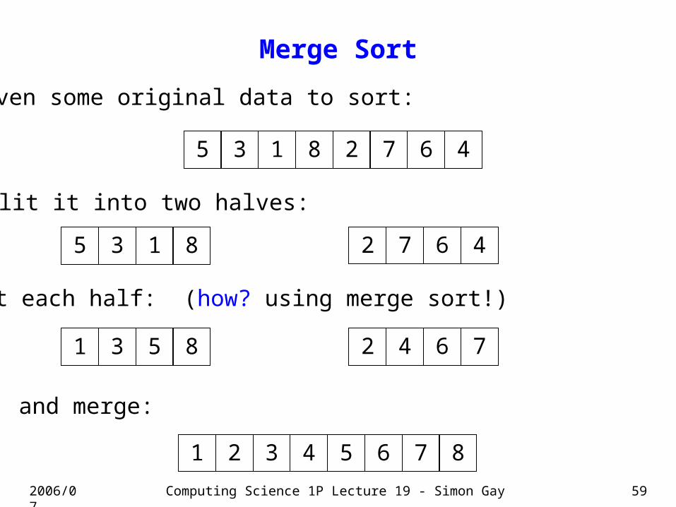
5 3 1 8 2 7 6 4
Given some original data to sort:
split it into two halves:
5 3 1 8 2 7 6 4
sort each half: (how? using merge sort!)
1 3 5 8 2 4 6 7
and merge:
1 2 3 4 5 6 7 8
2006/07 Computing Science 1P Lecture 19 - Simon Gay 60
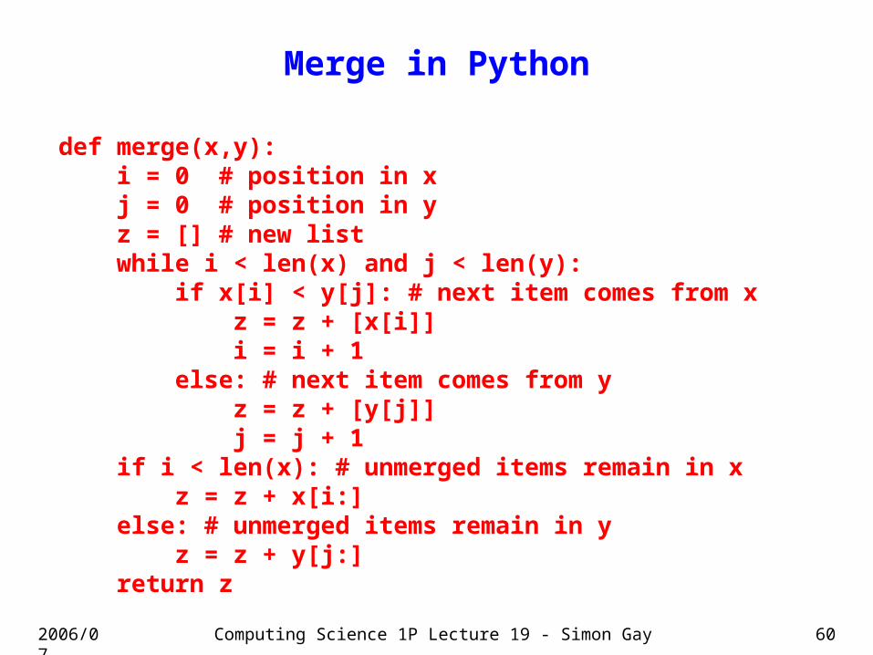
Merge in Python
def merge(x,y): i = 0 # position in x j = 0 # position in y z = [] # new list while i < len(x) and j < len(y): if x[i] < y[j]: # next item comes from x z = z + [x[i]] i = i + 1 else: # next item comes from y z = z + [y[j]] j = j + 1 if i < len(x): # unmerged items remain in x z = z + x[i:] else: # unmerged items remain in y z = z + y[j:] return z
2006/07 Computing Science 1P Lecture 19 - Simon Gay 61
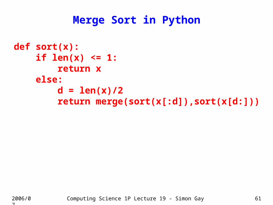
Merge Sort in Python
def sort(x): if len(x) <= 1: return x else: d = len(x)/2 return merge(sort(x[:d]),sort(x[d:]))

2006/07 Computing Science 1P Lecture 19 - Simon Gay 62
Analyzing Merge Sort
The algorithm repeatedly splits lists in half, sorts them, thenmerges the results. All the comparisons are in the merging.
Think of it like this:
merge
merge
merge
length n
length n/2
length n/4
length 1
…

2006/07 Computing Science 1P Lecture 19 - Simon Gay 63
Analyzing Merge Sort
Merging to produce a list of length n requires n-1 comparisons.The important thing is that this is order n.
Each round of merging requires n comparisons in total(not exactly, but we only care about the fact that it is n not n²or something else).
How many rounds of merging are there? Easiest to see if n is apower of 2:
n = 8, 3 roundsn = 16, 4 roundsn = 32, 5 roundsand so on
the number of rounds is log n(meaning logarithm to base 2)

2006/07 Computing Science 1P Lecture 19 - Simon Gay 64
Analyzing Merge Sort
There are log n rounds of merging, each requiring ncomparisons. We say that merge sort has order n log n.

2006/07 Computing Science 1P Lecture 19 - Simon Gay 65
Comparing Selection Sort and Merge SortWe now know that selection sort has order n²and merge sort has order n log n.
n n log n time n² time
10 33 100
100 664 10 000
1 000 9966 0.01 sec 1 million 1 sec
10 000 132 877 0.1 sec 100 million 100 sec
100 000 1.6 million 1.6 sec 10 billion 3 hours
1 000 000 20 million 20 sec 1 trillion 4 months
10 000 000 230 million 4 min 100 trillion 3 million yrs

2006/07 Computing Science 1P Lecture 19 - Simon Gay 66
Conclusion
There are usually many algorithms for a given problem; someare more efficient than others; the difference can have hugepractical significance.
The subject of algorithm analysis is a large area of CS. It willcome back later in the degree, especially in Levels 3 and 4.
Even for the problem of sorting, there is much more to saythan the fact that merge sort is better than selection sort.It is possible to prove that we can't do better than n log n,unless the data has special properties.