Computing Scheme of Work Year 6 Spreadsheets Crash course

Computing Scheme of Work

Year 6 Spreadsheets Crash course

For pupils in year 6 who have not used

2Calculate previously.

Year 6 Spreadsheet Catch-Up Contents

Need more support? Contact us:

Tel: +44(0)208 203 1781 | Email: [email protected] | Twitter: @2simplesoftware

2

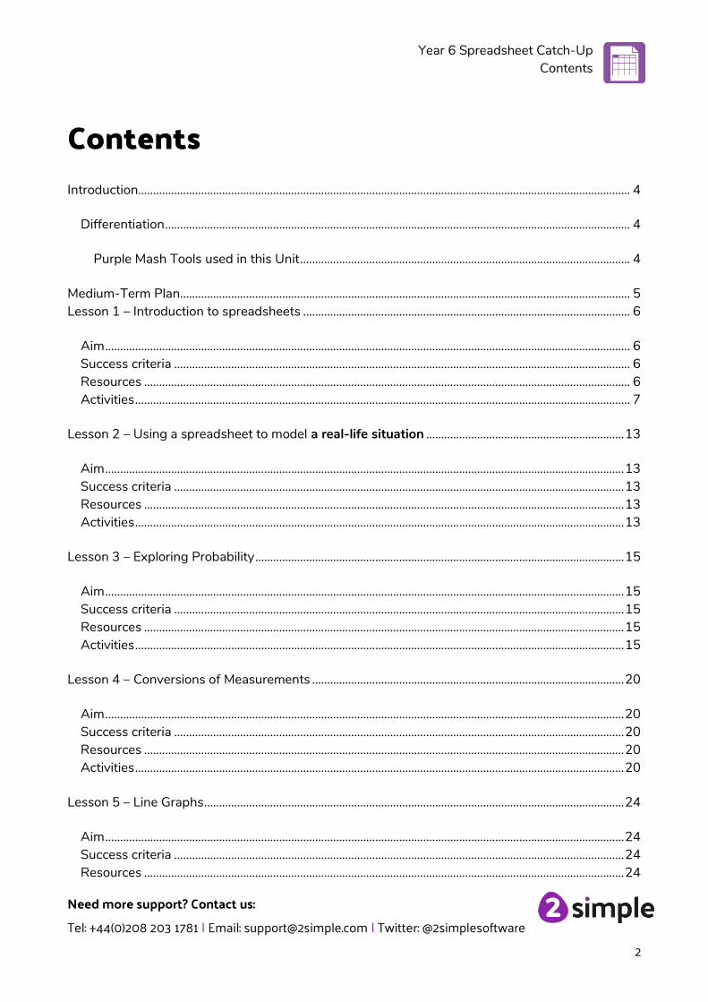
Contents

Introduction.................................................................................................................................................................... 4

Differentiation ........................................................................................................................................................... 4

Purple Mash Tools used in this Unit .............................................................................................................. 4

Medium-Term Plan ...................................................................................................................................................... 5

Lesson 1 – Introduction to spreadsheets ............................................................................................................. 6

Aim ............................................................................................................................................................................... 6

Success criteria ........................................................................................................................................................ 6

Resources .................................................................................................................................................................. 6

Activities ..................................................................................................................................................................... 7

Lesson 2 – Using a spreadsheet to model a real-life situation .................................................................. 13

Aim ............................................................................................................................................................................. 13

Success criteria ...................................................................................................................................................... 13

Resources ................................................................................................................................................................ 13

Activities ................................................................................................................................................................... 13

Lesson 3 – Exploring Probability ........................................................................................................................... 15

Aim ............................................................................................................................................................................. 15


Resources ................................................................................................................................................................ 15

Activities ................................................................................................................................................................... 15

Lesson 4 – Conversions of Measurements ........................................................................................................ 20

Aim ............................................................................................................................................................................. 20


Resources ................................................................................................................................................................ 20

Activities ................................................................................................................................................................... 20

Lesson 5 – Line Graphs ............................................................................................................................................ 24

Aim ............................................................................................................................................................................. 24


Resources ................................................................................................................................................................ 24

Year 6 Spreadsheet Catch-Up Contents



3

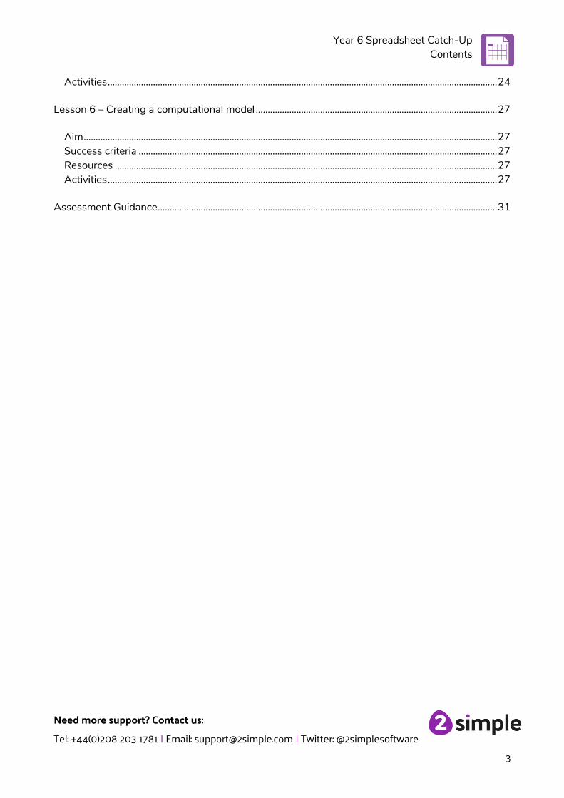
Activities ................................................................................................................................................................... 24

Lesson 6 – Creating a computational model ..................................................................................................... 27

Aim ............................................................................................................................................................................. 27


Resources ................................................................................................................................................................ 27

Activities ................................................................................................................................................................... 27

Assessment Guidance .............................................................................................................................................. 31

Year 6 Spreadsheet Catch-Up Introduction



4

Introduction 2Calculate is a simple to use spreadsheet (and more!) for beginners and beyond. A user guide can be found at 2Calculate User Guide. The following guide contains a catch-up unit of work forming part of the Computing Scheme of Work for teaching the use of spreadsheets. It is aimed at classes in which the pupils have not used 2Calculate before. This unit is one session longer than the scheme of work unit 6.3. The lessons assume that pupils are logged onto Purple Mash with their own individual usernames and passwords, so their work will be saved in their own folders automatically and can be easily reviewed and assessed by the class teacher. If you are currently using a single login per class or group and would like to set up individual logins yourself, then please see our guide to doing so at Create and Mange Users. Alternatively, please contact support at [email protected] or 0208 203 1781.

Differentiation

If pupils are not familiar with computer keyboards and mice and are going to be using 2Calculate on computers rather than tablets, then they would benefit from doing some work to familiarise themselves with the keys such as the arrow keys, enter and space. The use of spreadsheets has a strong link to mathematics. Some pupils might have difficulty with the mathematical concepts in some lessons and might need guidance with this aspect. For example, in lessons where spreadsheets are being used to add up prices; pupils who are not familiar with converting pence (45p) to pounds (£0.45) might need this aspect explained in more details; in lessons dealing with percentages and fractions some pupils might need extra support for the mathematical concepts. Where appropriate, guidance has been given on how to simplify tasks within lessons or challenge those who are ready for more stretching tasks.

Purple Mash Tools used in this Unit

2Calculate

https://www.purplemash.com/site#tab/teachers/guides_and_resources/2calculate_resources

https://www.purplemash.com/manuals/manageusers/index.html

mailto:[email protected]

Year 6 Spreadsheet Catch-Up Medium-Term Plan



5

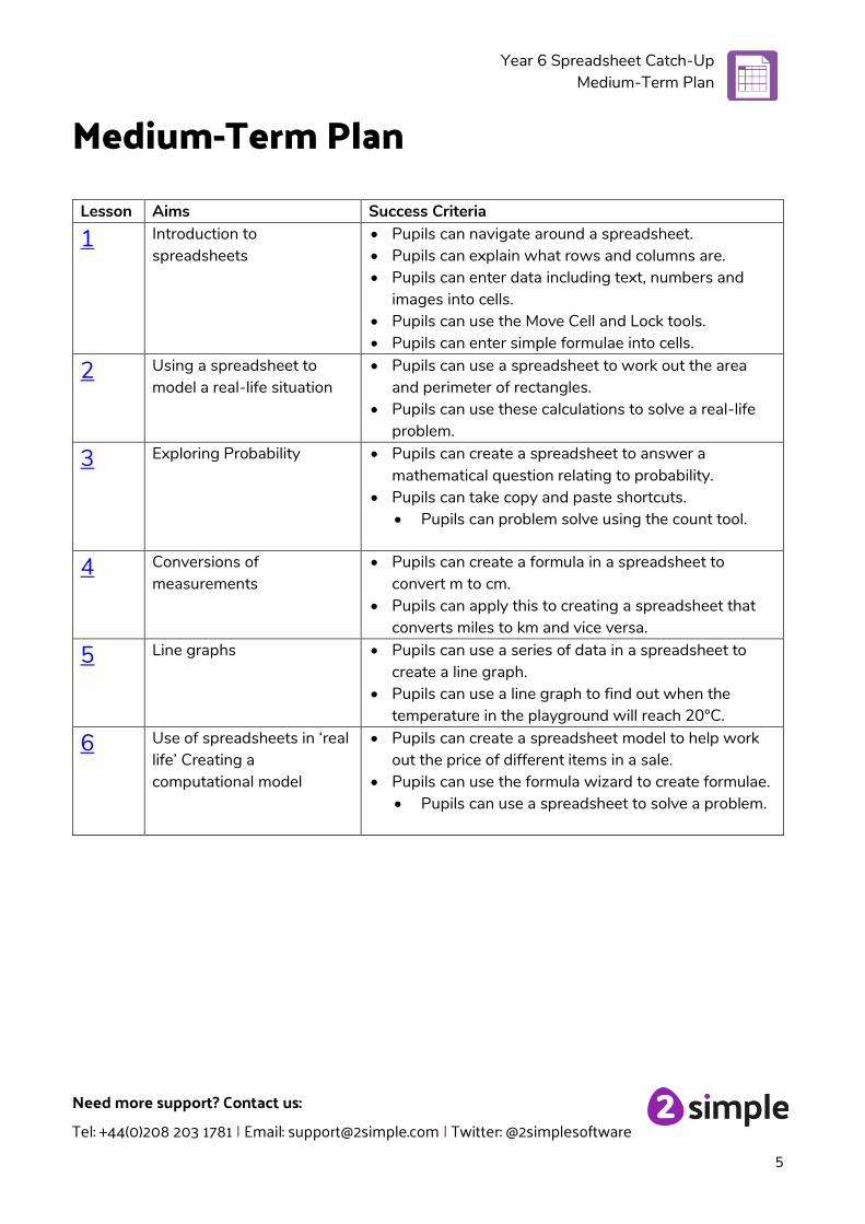
Medium-Term Plan Lesson Aims Success Criteria

1

Introduction to spreadsheets

• Pupils can navigate around a spreadsheet. • Pupils can explain what rows and columns are. • Pupils can enter data including text, numbers and

images into cells. • Pupils can use the Move Cell and Lock tools. • Pupils can enter simple formulae into cells.

2

Using a spreadsheet to model a real-life situation

• Pupils can use a spreadsheet to work out the area and perimeter of rectangles.

• Pupils can use these calculations to solve a real-life problem.

3

Exploring Probability • Pupils can create a spreadsheet to answer a mathematical question relating to probability.

• Pupils can take copy and paste shortcuts. • Pupils can problem solve using the count tool.

4

Conversions of measurements

• Pupils can create a formula in a spreadsheet to convert m to cm.

• Pupils can apply this to creating a spreadsheet that converts miles to km and vice versa.

5 Line graphs • Pupils can use a series of data in a spreadsheet to create a line graph.

• Pupils can use a line graph to find out when the temperature in the playground will reach 20°C.

6 Use of spreadsheets in ‘real life’ Creating a computational model

• Pupils can create a spreadsheet model to help work out the price of different items in a sale.

• Pupils can use the formula wizard to create formulae. • Pupils can use a spreadsheet to solve a problem.

Year 6 Spreadsheet Catch-Up Lesson 2



6

Lesson 1 – Introduction to spreadsheets

Aim

• To know what a spreadsheet looks like. • To be able to navigate around a spreadsheet and enter data. • To learn new vocabulary related to spreadsheets. • To add a variety of data types to a spreadsheet. • To use the ‘move cell’ and ‘lock’ tools. • To perform simple calculations.

Success criteria

• Pupils can navigate around a spreadsheet. • Pupils can explain what rows and columns are. • Pupils can insert text, numbers and images into cells. • Pupils can use the appropriate tools to drag and lock cells. • Pupils understand that formulae can be used to perform calculations within a spreadsheet. • Pupils can enter data into cells.

Resources

Unless otherwise stated, all resources can be found on the main unit 6.3 page. From here, click on the icon to set a resource as a 2do for your class. Use the links below to preview the resources; right-click on the link and ‘open in new tab’ so you don’t lose this page.

• 2Calculate prompt sheet to display on the whiteboard. • Copying and Pasting help sheet – this can be used if pupils are not familiar with how to copy

and paste using keyboard shortcuts or on a tablet.

Note for teacher: In this lesson, pupils are introduced to a variety of tools and time is given to allowing them to try out each in turn. Determine the time spent dependent upon the time that you have available. Alternatively, demonstrate the functions and then display the prompt sheet to help pupils then explore on their own.

https://www.purplemash.com/#tab/Teachers/computing_sow/computing_sow_y6/computing_sow_y6_unit_6-3

https://www.purplemash.com/app/schemes_of_work/computing_schemes_of_work/computing_sow_year2_unit_2_3_prompt_sheet

https://www.purplemash.com/app/schemes_of_work/computing_schemes_of_work/computing_sow_year2_unit_2_3_copying_pasting




7

Activities

1. Explain to the pupils that we are looking at a type of computer program called a spreadsheet today. Spreadsheets are used for organising information. For example, if you were planning a tea party you could input to the spreadsheet all the things you will need to get for the party and who you were going to invite. Can they think of any other things that could be stored in a spreadsheet for organising a party? (menus, gift list, entertainments).

2. Many people make lists on paper but the advantage of using a spreadsheet is that it can also do calculations for you. Explain what this means e.g. you could enter the cost of the different things that you will need for your party into the spreadsheet and then easily calculate how much money you will need to buy them all.

3. The aim today is to open a spreadsheet program in Purple Mash called 2Calculate and to learn how to enter information and do some simple calculations.

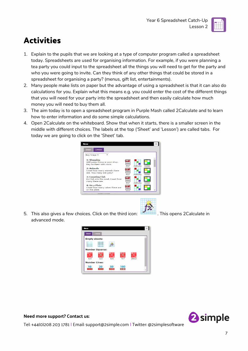
4. Open 2Calculate on the whiteboard. Show that when it starts, there is a smaller screen in the middle with different choices. The labels at the top (‘Sheet’ and ‘Lesson’) are called tabs. For today we are going to click on the ‘Sheet’ tab.

5. This also gives a few choices. Click on the third icon: . This opens 2Calculate in advanced mode.




8

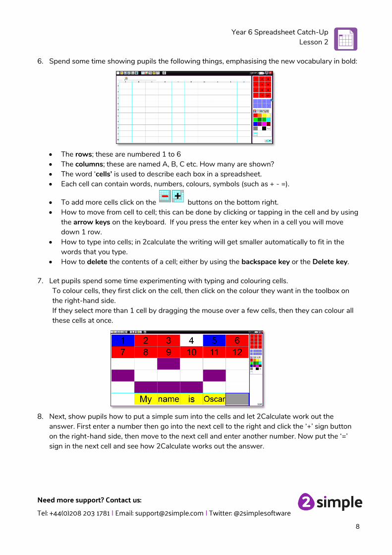
6. Spend some time showing pupils the following things, emphasising the new vocabulary in bold:

• The rows; these are numbered 1 to 6 • The columns; these are named A, B, C etc. How many are shown? • The word ‘cells’ is used to describe each box in a spreadsheet. • Each cell can contain words, numbers, colours, symbols (such as + - =).

• To add more cells click on the buttons on the bottom right. • How to move from cell to cell; this can be done by clicking or tapping in the cell and by using

the arrow keys on the keyboard. If you press the enter key when in a cell you will move down 1 row.

• How to type into cells; in 2calculate the writing will get smaller automatically to fit in the words that you type.

• How to delete the contents of a cell; either by using the backspace key or the Delete key.

7. Let pupils spend some time experimenting with typing and colouring cells. To colour cells, they first click on the cell, then click on the colour they want in the toolbox on the right-hand side. If they select more than 1 cell by dragging the mouse over a few cells, then they can colour all these cells at once.

8. Next, show pupils how to put a simple sum into the cells and let 2Calculate work out the answer. First enter a number then go into the next cell to the right and click the ‘+’ sign button on the right-hand side, then move to the next cell and enter another number. Now put the ‘=’ sign in the next cell and see how 2Calculate works out the answer.




9

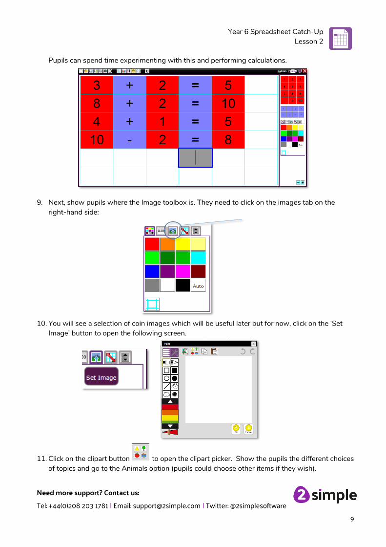
Pupils can spend time experimenting with this and performing calculations.

9. Next, show pupils where the Image toolbox is. They need to click on the images tab on the right-hand side:

10. You will see a selection of coin images which will be useful later but for now, click on the ‘Set Image’ button to open the following screen.

11. Click on the clipart button to open the clipart picker. Show the pupils the different choices of topics and go to the Animals option (pupils could choose other items if they wish).




10

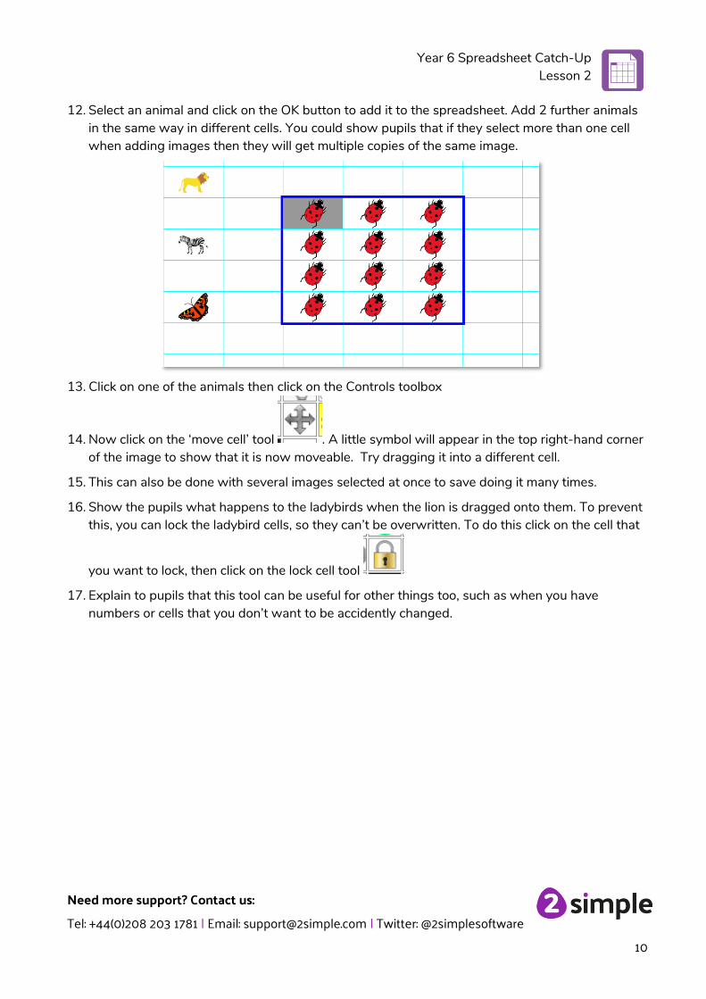
12. Select an animal and click on the OK button to add it to the spreadsheet. Add 2 further animals in the same way in different cells. You could show pupils that if they select more than one cell when adding images then they will get multiple copies of the same image.

13. Click on one of the animals then click on the Controls toolbox

14. Now click on the ‘move cell’ tool . A little symbol will appear in the top right-hand corner of the image to show that it is now moveable. Try dragging it into a different cell.

15. This can also be done with several images selected at once to save doing it many times.

16. Show the pupils what happens to the ladybirds when the lion is dragged onto them. To prevent this, you can lock the ladybird cells, so they can’t be overwritten. To do this click on the cell that

you want to lock, then click on the lock cell tool

17. Explain to pupils that this tool can be useful for other things too, such as when you have numbers or cells that you don’t want to be accidently changed.




11

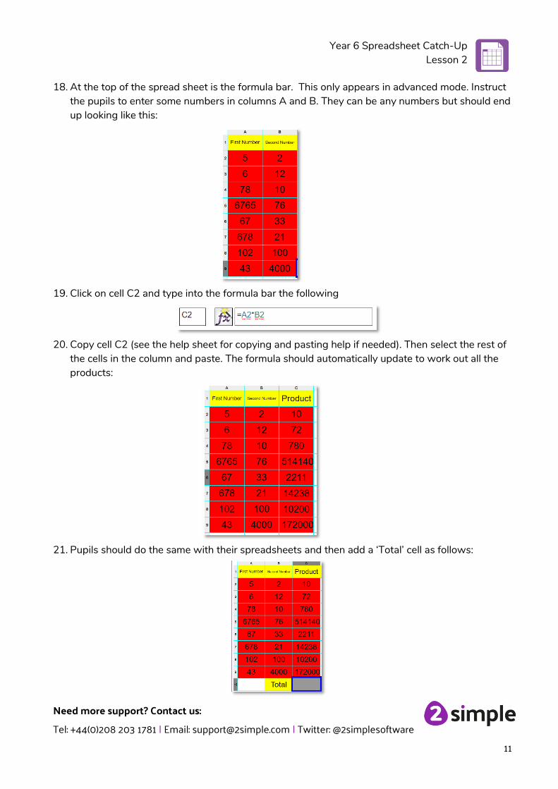
18. At the top of the spread sheet is the formula bar. This only appears in advanced mode. Instruct the pupils to enter some numbers in columns A and B. They can be any numbers but should end up looking like this:

19. Click on cell C2 and type into the formula bar the following

20. Copy cell C2 (see the help sheet for copying and pasting help if needed). Then select the rest of the cells in the column and paste. The formula should automatically update to work out all the products:

21. Pupils should do the same with their spreadsheets and then add a ‘Total’ cell as follows:




12

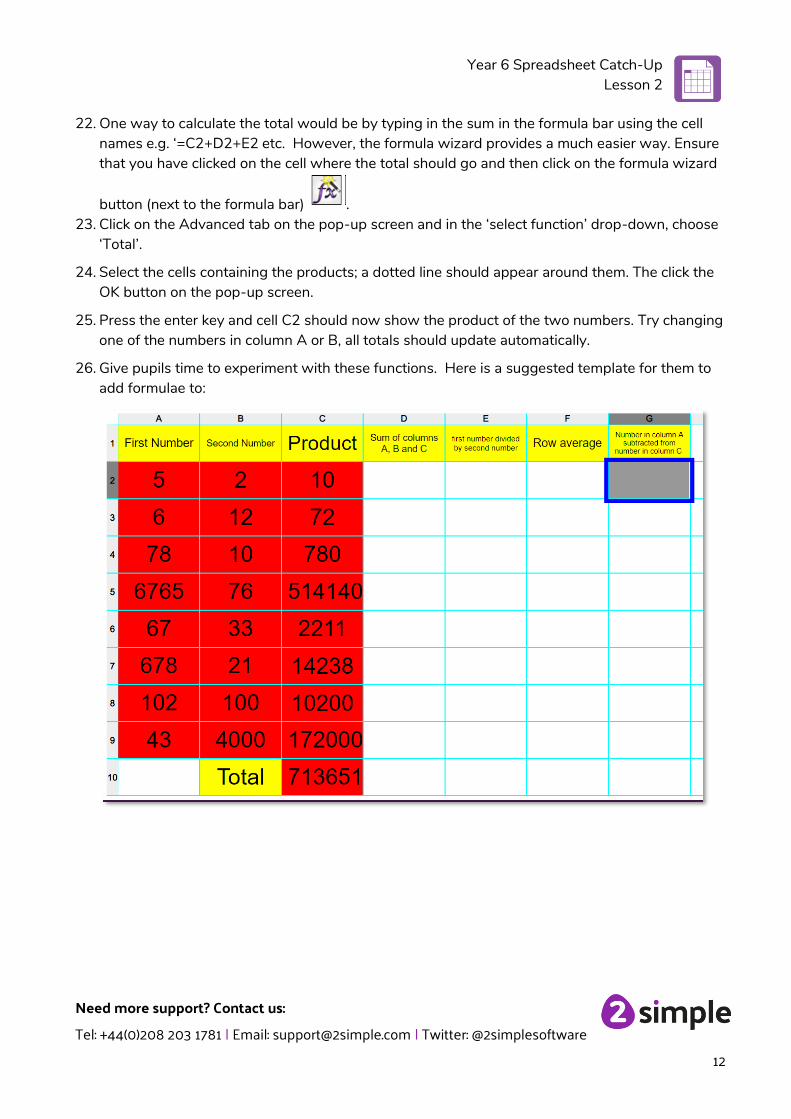
22. One way to calculate the total would be by typing in the sum in the formula bar using the cell names e.g. ‘=C2+D2+E2 etc. However, the formula wizard provides a much easier way. Ensure that you have clicked on the cell where the total should go and then click on the formula wizard

button (next to the formula bar) . 23. Click on the Advanced tab on the pop-up screen and in the ‘select function’ drop-down, choose

‘Total’.

24. Select the cells containing the products; a dotted line should appear around them. The click the OK button on the pop-up screen.

25. Press the enter key and cell C2 should now show the product of the two numbers. Try changing one of the numbers in column A or B, all totals should update automatically.

26. Give pupils time to experiment with these functions. Here is a suggested template for them to add formulae to:




13

Lesson 2 – Using a spreadsheet to model a real-life situation

Aim

• To use a spreadsheet to model a real-life problem • To use formulae to calculate area and perimeter of shapes.

Success criteria

• Pupils can use a spreadsheet to work out the area and perimeter of rectangles. • Pupils can use these calculations to solve a real-life problem.

Resources


• Cuboids example

Activities

1. Modelling in Computing means creating or using a model or simulation of a real-life situation, on a computer. For example, we could start by creating a page in 2calculate which added up how much money we made by selling 3 pizzas for 25p and 2 apples for 10p each in the school tuck shop. We could then use 2calculate to explore what would happen if we changed parts of the model—by putting up the prices for example. Changing certain values within the page and seeing what happens is what is meant by modelling.


https://www.purplemash.com/app/pup/sow_y5_Lcuboids




14

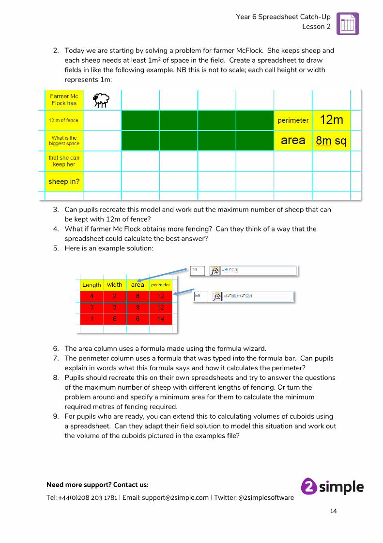
2. Today we are starting by solving a problem for farmer McFlock. She keeps sheep and each sheep needs at least 1m² of space in the field. Create a spreadsheet to draw fields in like the following example. NB this is not to scale; each cell height or width represents 1m:

3. Can pupils recreate this model and work out the maximum number of sheep that can be kept with 12m of fence?

4. What if farmer Mc Flock obtains more fencing? Can they think of a way that the spreadsheet could calculate the best answer?

5. Here is an example solution:

6. The area column uses a formula made using the formula wizard. 7. The perimeter column uses a formula that was typed into the formula bar. Can pupils

explain in words what this formula says and how it calculates the perimeter? 8. Pupils should recreate this on their own spreadsheets and try to answer the questions

of the maximum number of sheep with different lengths of fencing. Or turn the problem around and specify a minimum area for them to calculate the minimum required metres of fencing required.

9. For pupils who are ready, you can extend this to calculating volumes of cuboids using a spreadsheet. Can they adapt their field solution to model this situation and work out the volume of the cuboids pictured in the examples file?




15

Lesson 3 – Exploring Probability

Aim

• To use a spreadsheet to investigate the probability of the results of throwing many dice.

Success criteria

• Pupils can create a spreadsheet to answer a mathematical question relating to probability. • Pupils can take copy and paste shortcuts. • Pupils can problem solve using the count tool.

Resources

• 2Calculate tool

Activities

1. Explain that the pupils are going to use the dice tool to try and work out the probability of throwing certain numbers.

2. Open a blank sheet in advanced view:

3. Remind the pupils how to make their spreadsheet bigger by clicking on the in the button on the bottom right of the screen to add more cells.

4. Initially, you will need a sheet that goes to row 11 and column J.

5. Create a sheet like the example below. The dice tool can be found in the controls toolbox:

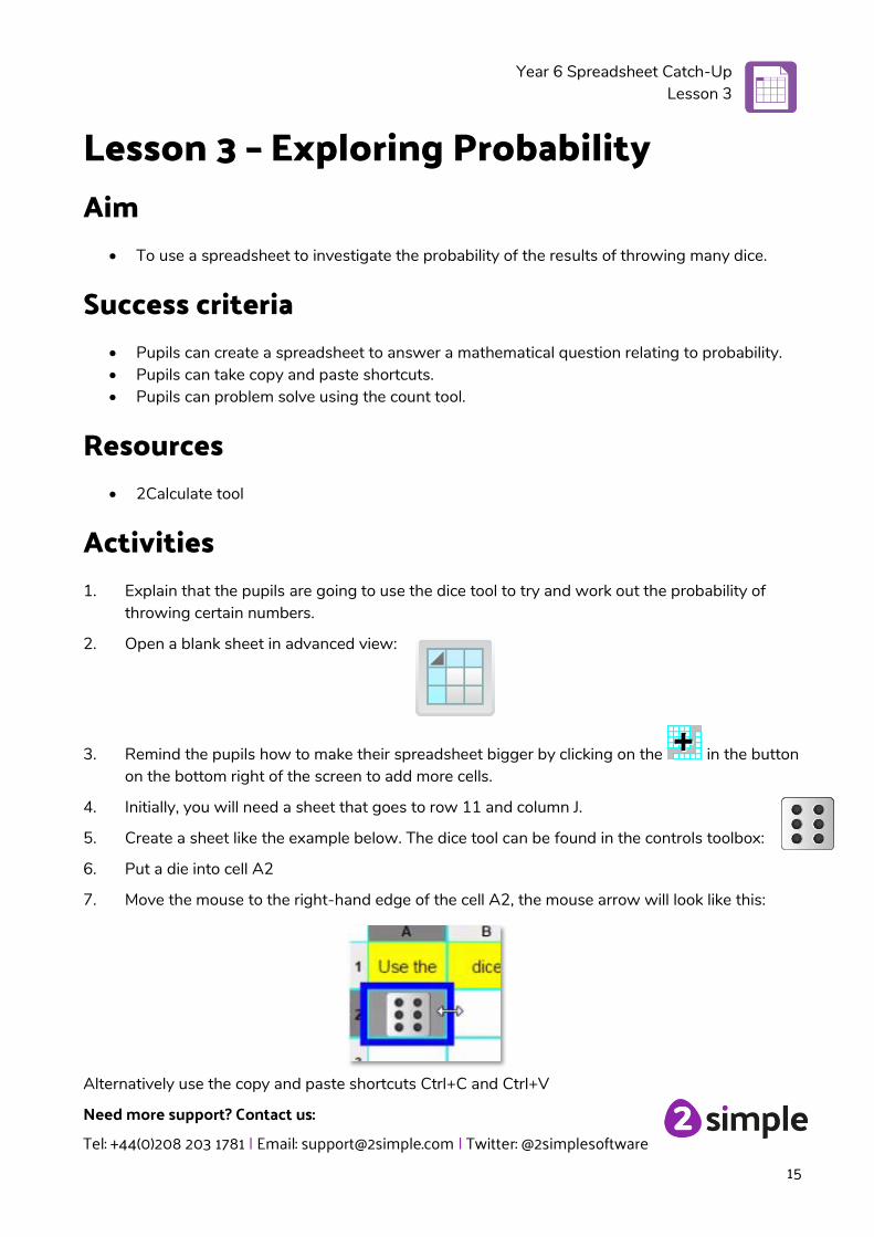
6. Put a die into cell A2

7. Move the mouse to the right-hand edge of the cell A2, the mouse arrow will look like this:

Alternatively use the copy and paste shortcuts Ctrl+C and Ctrl+V




16

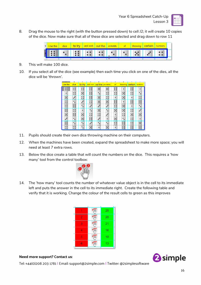
8. Drag the mouse to the right (with the button pressed down) to cell J2; it will create 10 copies of the dice. Now make sure that all of these dice are selected and drag down to row 11

9. This will make 100 dice.

10. If you select all of the dice (see example) then each time you click on one of the dies, all the dice will be ‘thrown’.

11. Pupils should create their own dice throwing machine on their computers.

12. When the machines have been created, expand the spreadsheet to make more space; you will need at least 7 extra rows.

13. Below the dice create a table that will count the numbers on the dice. This requires a ‘how many’ tool from the control toolbox:

14. The ‘how many’ tool counts the number of whatever value object is in the cell to its immediate left and puts the answer in the cell to its immediate right. Create the following table and verify that it is working. Change the colour of the result cells to green as this improves




17

accuracy due to the way the count toll works. The total should add up to 100 as there are 100 dice. The numbers should change each time the die is thrown.

15. Start to look at the results. Is any number more likely than the others? Is this answer correct if we change the numbers rolled?

16. Further Questions:

• Q How likely is it we will roll a 4?

• Q How likely we will roll a 0?

• Q How likely is it we will roll a 7?

• Q Are we more likely to roll an odd or an even number?

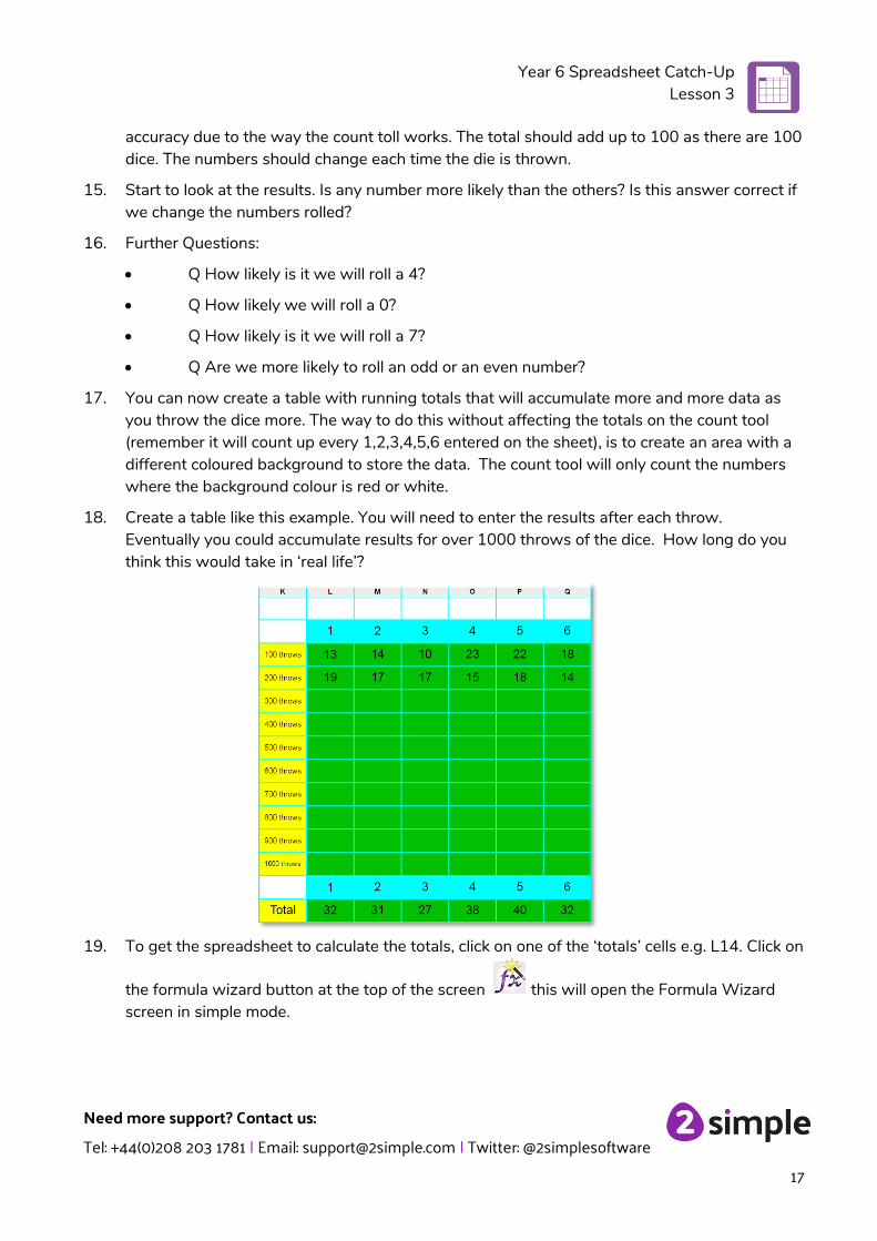
17. You can now create a table with running totals that will accumulate more and more data as you throw the dice more. The way to do this without affecting the totals on the count tool (remember it will count up every 1,2,3,4,5,6 entered on the sheet), is to create an area with a different coloured background to store the data. The count tool will only count the numbers where the background colour is red or white.

18. Create a table like this example. You will need to enter the results after each throw. Eventually you could accumulate results for over 1000 throws of the dice. How long do you think this would take in ‘real life’?

19. To get the spreadsheet to calculate the totals, click on one of the ‘totals’ cells e.g. L14. Click on

the formula wizard button at the top of the screen this will open the Formula Wizard screen in simple mode.




18

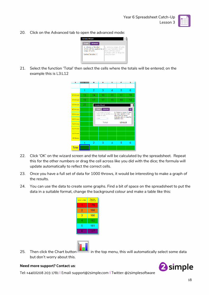
20. Click on the Advanced tab to open the advanced mode:

21. Select the function ‘Total’ then select the cells where the totals will be entered; on the example this is L3:L12

22. Click ‘OK’ on the wizard screen and the total will be calculated by the spreadsheet. Repeat this for the other numbers or drag the cell across like you did with the dice; the formula will update automatically to reflect the correct cells.

23. Once you have a full set of data for 1000 throws, it would be interesting to make a graph of the results.

24. You can use the data to create some graphs. Find a bit of space on the spreadsheet to put the data in a suitable format, change the background colour and make a table like this:

25. Then click the Chart button in the top menu, this will automatically select some data but don’t worry about this.




19

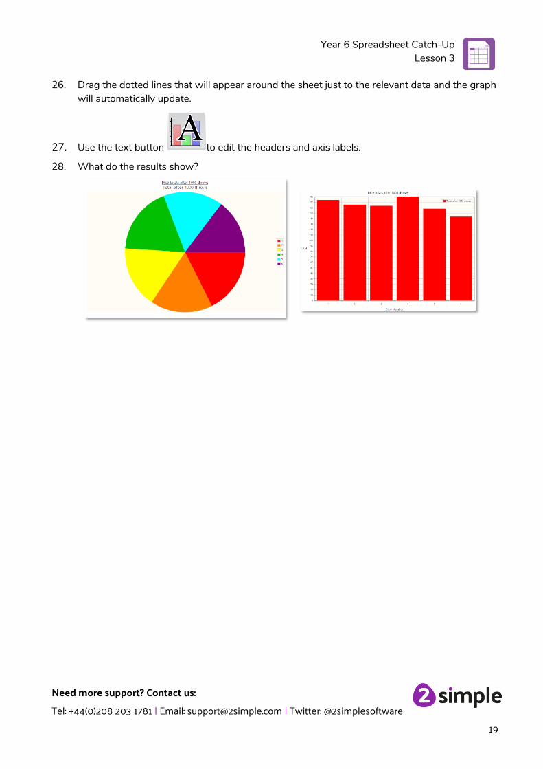
26. Drag the dotted lines that will appear around the sheet just to the relevant data and the graph will automatically update.

27. Use the text button to edit the headers and axis labels.

28. What do the results show?




20

Lesson 4 – Conversions of Measurements

Aim

• To use formulae within a spreadsheet to convert measurements of length and distance.

Success criteria

• Pupils can create a formula in a spreadsheet to convert m to cm. • Pupils can apply this to creating a spreadsheet that converts miles to km and vice

versa.

Resources


• Conversion example spreadsheet.

Note for teachers; in step 13, pupils use keyboard shortcuts for copying and pasting. If pupils are using tablets then the method is different, both methods are detailed in the resource file Copying and Pasting that can be displayed on the whiteboard.

Activities

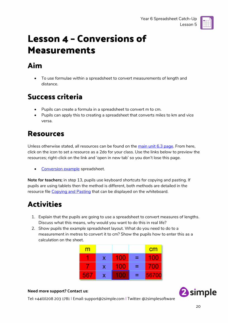
1. Explain that the pupils are going to use a spreadsheet to convert measures of lengths. Discuss what this means, why would you want to do this in real life?

2. Show pupils the example spreadsheet layout. What do you need to do to a measurement in metres to convert it to cm? Show the pupils how to enter this as a calculation on the sheet.


https://www.purplemash.com/#app/pup/sow_y5_L1

https://www.purplemash.com/app/schemes_of_work/computing_schemes_of_work/computing_sow_year2_unit_2_3_copying_pasting




21

3. Ask pupils to use the same format to convert from cm to m on their own sheets. (Use the advanced format sheet).

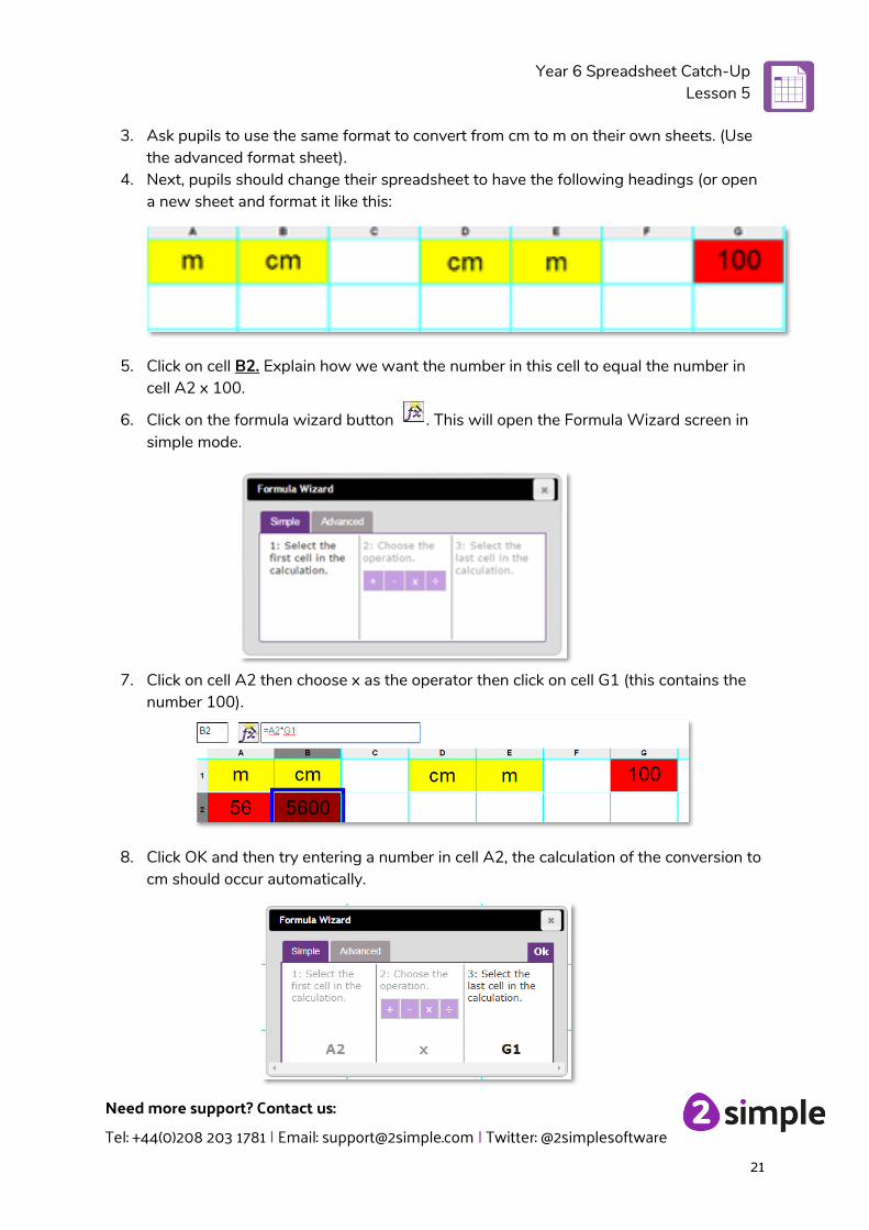
4. Next, pupils should change their spreadsheet to have the following headings (or open a new sheet and format it like this:

5. Click on cell B2. Explain how we want the number in this cell to equal the number in cell A2 x 100.

6. Click on the formula wizard button . This will open the Formula Wizard screen in simple mode.

7. Click on cell A2 then choose x as the operator then click on cell G1 (this contains the number 100).

8. Click OK and then try entering a number in cell A2, the calculation of the conversion to cm should occur automatically.




22

9. Ask pupils to create a similar formula for the other cells in column B on their own spreadsheets and test it out by entering different values in column A.

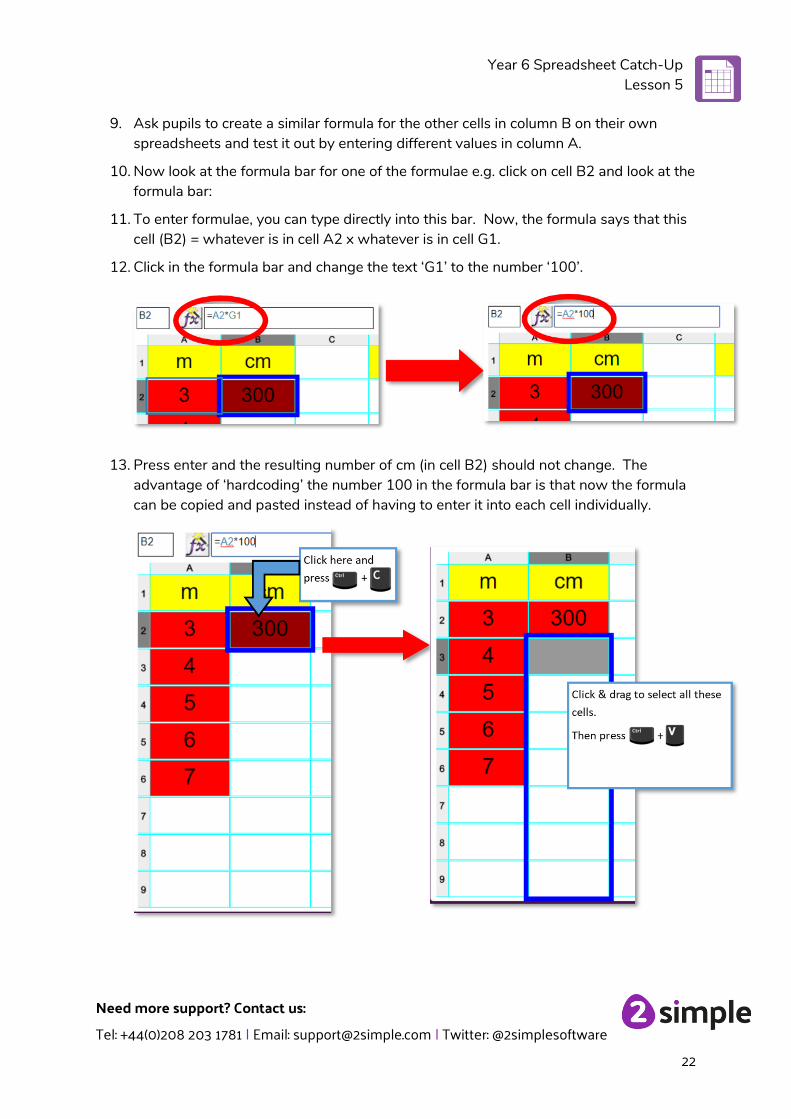
10. Now look at the formula bar for one of the formulae e.g. click on cell B2 and look at the formula bar:

11. To enter formulae, you can type directly into this bar. Now, the formula says that this cell (B2) = whatever is in cell A2 x whatever is in cell G1.

12. Click in the formula bar and change the text ‘G1’ to the number ‘100’.

13. Press enter and the resulting number of cm (in cell B2) should not change. The

advantage of ‘hardcoding’ the number 100 in the formula bar is that now the formula can be copied and pasted instead of having to enter it into each cell individually.




23

14. Copy cell B2 (click on cell B6 then press + . Now select the rest of column

B and then paste + . This should copy the formula and automatically update it to each row. The rows where column A is empty should initially display zeros. Test this out by entering numbers into the cells in column A.

15. See if pupils can use this method to create a formula that takes the contents on the cells in column D and divides by 100 to convert from cm to m.

16. NB They will need to use the ‘/’ key for a divide sign.

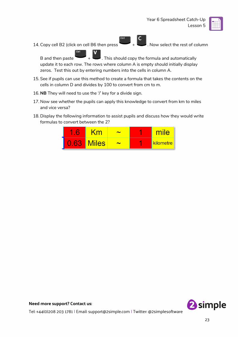
17. Now see whether the pupils can apply this knowledge to convert from km to miles and vice versa?

18. Display the following information to assist pupils and discuss how they would write formulas to convert between the 2?




24

Lesson 5 – Line Graphs

Aim

• To use the line graphing tool in 2Calculate with appropriate data. • To interpret a line graph to estimate values between data readings.

Success criteria

• Pupils can use a series of data in a spreadsheet to create a line graph. • Pupils can use a line graph to find out when the temperature in the playground will reach

20°C.

Resources


• Line Graph Example Data photo; the lesson uses example data; you could collect similar real data in advance of the lesson to make the activity more relevant to the pupils.

Activities

1. Create a blank worksheet by clicking on the new page icon at the top left of the screen.

2. You will probably have to resize the spreadsheet using the buttons in order to fit in the data. These buttons can be pressed at any time if you are running out of space and then the data can be copied and pasted into different cells if necessary.

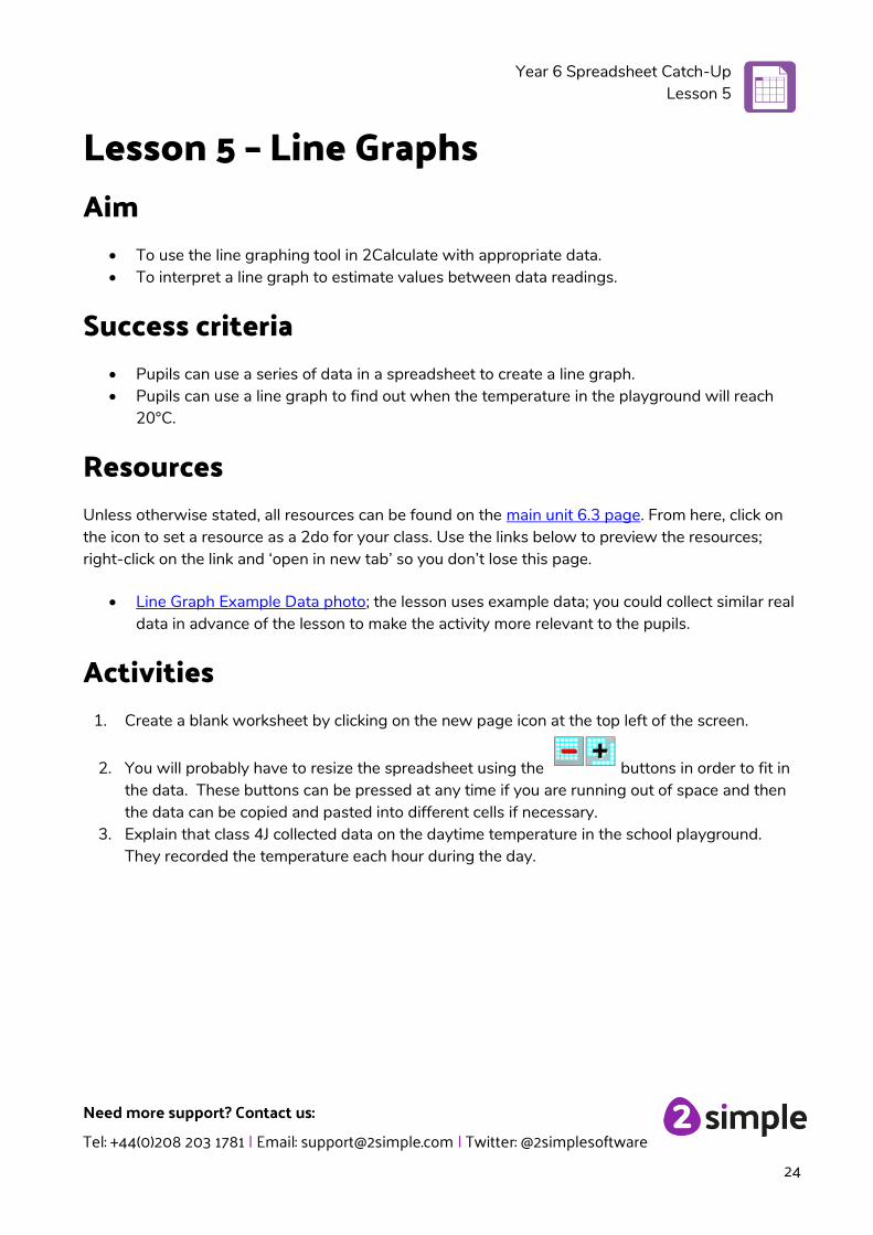
3. Explain that class 4J collected data on the daytime temperature in the school playground. They recorded the temperature each hour during the day.


https://www.purplemash.com/#app/pup/sow_2calc_y4_l3_data




25

4. Here is their record of the data (this photo is linked to above for displaying on a whiteboard):

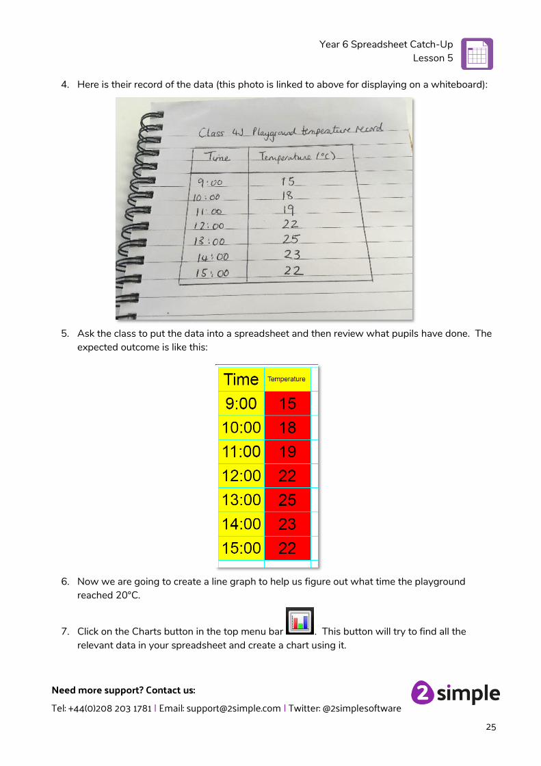
5. Ask the class to put the data into a spreadsheet and then review what pupils have done. The expected outcome is like this:

6. Now we are going to create a line graph to help us figure out what time the playground reached 20°C.

7. Click on the Charts button in the top menu bar . This button will try to find all the relevant data in your spreadsheet and create a chart using it.




26

8. If the tool does not find all your data, you can drag the dotted lines (that will appear) to select the data that you want to include in your chart.

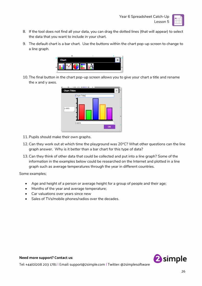
9. The default chart is a bar chart. Use the buttons within the chart pop-up screen to change to a line graph.

10. The final button in the chart pop-up screen allows you to give your chart a title and rename the x and y axes.

11. Pupils should make their own graphs.

12. Can they work out at which time the playground was 20°C? What other questions can the line graph answer. Why is it better than a bar chart for this type of data?

13. Can they think of other data that could be collected and put into a line graph? Some of the information in the examples below could be researched on the Internet and plotted in a line graph such as average temperatures through the year in different countries.

Some examples;

• Age and height of a person or average height for a group of people and their age; • Months of the year and average temperature; • Car valuations over years since new • Sales of TVs/mobile phones/radios over the decades.

Year 6 Spreadsheet Catch-Up Assessment Guidance



27

Lesson 6 – Creating a computational model

Aim

• Use a spreadsheet to calculate the discount and final prices in a sale. Create a formula to help work out the prices of items in the sale

Success criteria

• Pupils can create a spreadsheet model to help work out the price of different items in a sale.

• Pupils can use the formula wizard to create formulae. • Pupils can use a spreadsheet to solve a problem.

Resources

• 2Calculate tool

Note: The challenges in this lesson get gradually harder. You might decide to only go to a certain point with your class, dependent upon their ability, or to set some of the harder questions as extension work for some pupils.

Activities

1. Modelling in Computing means creating or using a simulation (a model) of a real life situation, on a computer. For example, we could start by creating a page in 2calculate which added up how much money we made by selling 3 pizzas for 25p and 2 apples for 10p each in the school tuck shop. We could then use 2Calculate to explore what would happen if we changed parts of the model—by putting up the prices for example. Changing certain values within the page and seeing what happens is what is meant by modelling.

2. Today we are going to make a model to help decide the best value tickets to buy for a concert.

3. Open a blank spreadsheet in Advanced view.




28

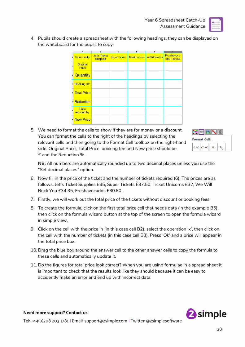
4. Pupils should create a spreadsheet with the following headings, they can be displayed on the whiteboard for the pupils to copy:

5. We need to format the cells to show if they are for money or a discount. You can format the cells to the right of the headings by selecting the relevant cells and then going to the Format Cell toolbox on the right-hand side. Original Price, Total Price, booking fee and New price should be £ and the Reduction %.

NB: All numbers are automatically rounded up to two decimal places unless you use the “Set decimal places” option.

6. Now fill in the price of the ticket and the number of tickets required (6). The prices are as follows: Jeffs Ticket Supplies £35, Super Tickets £37.50, Ticket Unicorns £32, We Will Rock You £34.35, Freshavocados £30.80.

7. Firstly, we will work out the total price of the tickets without discount or booking fees.

8. To create the formula, click on the first total price cell that needs data (in the example B5), then click on the formula wizard button at the top of the screen to open the formula wizard in simple view.

9. Click on the cell with the price in (in this case cell B2), select the operation ‘x’, then click on the cell with the number of tickets (in this case cell B3). Press ‘Ok’ and a price will appear in the total price box.

10. Drag the blue box around the answer cell to the other answer cells to copy the formula to these cells and automatically update it.

11. Do the figures for total price look correct? When you are using formulae in a spread sheet it is important to check that the results look like they should because it can be easy to accidently make an error and end up with incorrect data.




29

12. Make a chart to the side to record the costings order so that you can see how the prices change:

You can make the ticket seller name draggable by selecting them and then

clicking on the ‘move’ tool in the objects toolbox Then you can drag the names around as the cost changes.

13. Super Tickets have a 10% discount now so update the spreadsheet to reflect this. Enter 0.1 in the Reduction cell for Super Tickets. The cells are formatted as % so this should display as 10%.

14. Now click on the cell for the Price reduced by (C7), click on the formula wizard, then the original price x the reduction. Press OK and you can see the discount.

15. To work out the new total, click on the relevant New Price cell (C8), then the formula wizard and enter (by clicking on the cells) Total Price – Price reduced by. Then click ‘OK’.

16. Now add the following additional price reductions:

Jeff’s Ticket Supplies 25%

Ticket Unicorns 5%

We Will Rock You 20%

Freshavacados 15%

17. How does this change who is the cheapest supplier?

18. You are all set to buy your tickets from Freshavocados but then you read the small print and find out that there is a £4 booking fee. Can you add this into the spreadsheet and change the formulae to see if this affects the price?

19. To change the formula, click on cell F5 (total price). The formula bar should display the formula like this:

20. Click in the formula bar then on the end, add the text ‘+F4’, press enter. The formula should have changed, and the amount should now be reflected in the ticket price.




30

21. Now you decide to check the small print for Jeff’s Ticket Supplies, and you find there is a £2 booking fee. Add this to the spreadsheet and update the formula for cell B5.

22. You are just about to pay for your tickets from Jeff when you suddenly realise that the booking fee says, ‘per ticket’! What do you have to do to the spreadsheet to reflect this? One possibility is to change the formula for cell B6 as follows:

23. You decide to check all the small print. We Will Rock You and Super Tickets have no booking fee; great! Add this to the spreadsheet.

24. Then you see that today only, Ticket Unicorns have a magical buy 2 get one free offer on tickets! Can you show this in the spreadsheet?

25. The easiest way might be to change the number of tickets you are buying as you will only have to pay for 4 tickets now as you will then get 2 free. What a bargain! Quickly buy your tickets before they all run out.




31

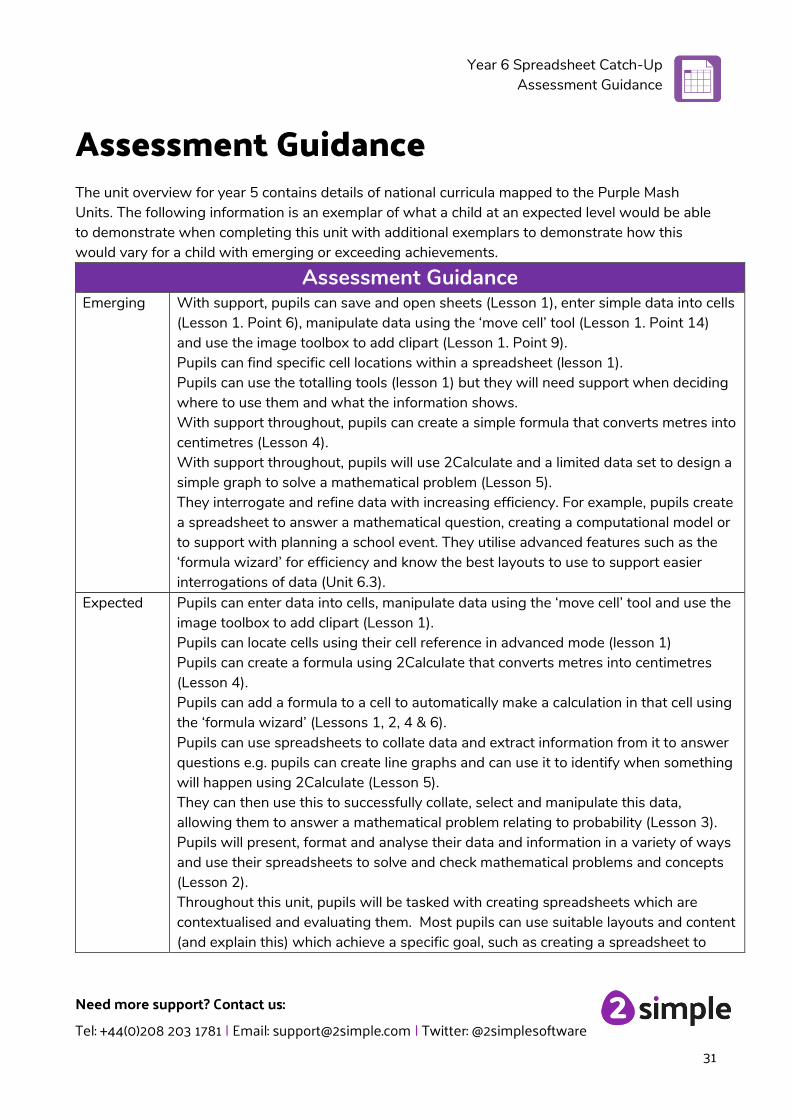
Assessment Guidance The unit overview for year 5 contains details of national curricula mapped to the Purple Mash Units. The following information is an exemplar of what a child at an expected level would be able to demonstrate when completing this unit with additional exemplars to demonstrate how this would vary for a child with emerging or exceeding achievements.

Assessment Guidance Emerging With support, pupils can save and open sheets (Lesson 1), enter simple data into cells

(Lesson 1. Point 6), manipulate data using the ‘move cell’ tool (Lesson 1. Point 14) and use the image toolbox to add clipart (Lesson 1. Point 9). Pupils can find specific cell locations within a spreadsheet (lesson 1). Pupils can use the totalling tools (lesson 1) but they will need support when deciding where to use them and what the information shows. With support throughout, pupils can create a simple formula that converts metres into centimetres (Lesson 4). With support throughout, pupils will use 2Calculate and a limited data set to design a simple graph to solve a mathematical problem (Lesson 5). They interrogate and refine data with increasing efficiency. For example, pupils create a spreadsheet to answer a mathematical question, creating a computational model or to support with planning a school event. They utilise advanced features such as the ‘formula wizard’ for efficiency and know the best layouts to use to support easier interrogations of data (Unit 6.3).

Expected Pupils can enter data into cells, manipulate data using the ‘move cell’ tool and use the image toolbox to add clipart (Lesson 1). Pupils can locate cells using their cell reference in advanced mode (lesson 1) Pupils can create a formula using 2Calculate that converts metres into centimetres (Lesson 4). Pupils can add a formula to a cell to automatically make a calculation in that cell using the ‘formula wizard’ (Lessons 1, 2, 4 & 6). Pupils can use spreadsheets to collate data and extract information from it to answer questions e.g. pupils can create line graphs and can use it to identify when something will happen using 2Calculate (Lesson 5). They can then use this to successfully collate, select and manipulate this data, allowing them to answer a mathematical problem relating to probability (Lesson 3). Pupils will present, format and analyse their data and information in a variety of ways and use their spreadsheets to solve and check mathematical problems and concepts (Lesson 2). Throughout this unit, pupils will be tasked with creating spreadsheets which are contextualised and evaluating them. Most pupils can use suitable layouts and content (and explain this) which achieve a specific goal, such as creating a spreadsheet to




32

Assessment Guidance work out the area and perimeter of rectangles Their layouts and contents will be fit for purpose for their intended audience.

Exceeding Pupils demonstrating greater depth will explore more complex functioning of the 2Calculate tools to create their own spreadsheets to explore number and interpret their own data. They will intuitively grasp the concept of using a spreadsheet to model a real-life situation and calculate solutions (lesson 6). Pupils demonstrating greater depth can use their understanding of converting metres into centimetres and apply this to other mathematical conversions (Lesson 4. Point 14 onwards) Furthermore, they choose the most appropriate way to convert and represent their data and can give their reasons behind this choice.

Computing Scheme of Work Year 6 Spreadsheets Crash course

Documents

Transcript of Computing Scheme of Work Year 6 Spreadsheets Crash course