Computers & Fluids 57 (2012) 208–224

Contents lists available at SciVerse ScienceDirect

Computers & Fluids

journal homepage: www.elsevier .com/locate /compfluid

A bounded upwinding scheme for computing convection-dominatedtransport problems

V.G. Ferreira a,⇑, R.A.B. de Queiroz a, G.A.B. Lima a, R.G. Cuenca a, C.M. Oishi b, J.L.F. Azevedo c, S. McKee d

a Departamento de Matemática Aplicada e Estatı́stica, Instituto de Ciências Matemáticas e de Computação – USP, São Carlos, SP, Brazilb Departamento de Matemática, Universidade Estadual Júlio de Mesquita Filho – UNESP, Presidente Prudente, SP, Brazilc Instituto de Aeronautica e Espaço, CTA/IAE/ALA, São José dos Campos, SP, Brazild Department of Mathematics and Statistics, University of Strathclyde, Glasgow, UK

a r t i c l e i n f o a b s t r a c t

Article history:Received 20 April 2009Received in revised form 26 September2011Accepted 27 December 2011Available online 10 January 2012

Keywords:Numerical simulationCBC/TVD stabilityHigh resolutionUpwindingMonotonic interpolationFinite differenceConvection modelingBoundedness

0045-7930/$ - see front matter � 2012 Elsevier Ltd. Adoi:10.1016/j.compfluid.2011.12.021

⇑ Corresponding author. Address: Av. TrabalhadorCEP: 13560-970, São Carlos, SP, Brazil.

E-mail address: pvgf@icmc.usp.br (V.G. Ferreira).

A practical high resolution upwind differencing scheme for the numerical solution of convection-domi-nated transport problems is presented. The scheme is based on TVD and CBC stability criteria and isimplemented in the context of the finite difference methodology. The performance of the scheme isinvestigated by solving the 1D/2D scalar advection equations, 1D inviscid Burgers’ equation, 1D scalarconvection–diffusion equation, 1D/2D compressible Euler’s equations, and 2D incompressible Navier–Stokes equations. The numerical results displayed good agreement with other existing numerical andexperimental data.

� 2012 Elsevier Ltd. All rights reserved.

1. Introduction

The development of fast, reliable and accurate numericalapproximations for the convection terms of hyperbolic conserva-tion laws and transport equations in fluid dynamics has presenteda continuing challenge. The most frustrating obstacle has been theattempt to prevent the unbounded growth of the unphysical spa-tial oscillations in the vicinity of sharp changes in gradients, orjump discontinuities. It is also essential that certain transport vari-ables remain bounded within physical limiting values. For exam-ple, the fluid depth in shallow water flows, the mixture fractionof reacting flows, the kinetic energy in turbulent flows, or speciesconcentration all cannot fall below zero. Previous studies by Smithand Hutton [54] (see also van Albada et al. [64] and van Leer [69])have shown that upwinding schemes may produce nonphysicalresults when boundedness is not preserved.

In order to obtain stable, bounded and physically plausible solu-tions, the classical first order upwind (FOU) difference scheme [21]– or the hybrid central upwind (HCU) [48,58] – is often adopted.

ll rights reserved.

São-carlense, 400 – Centro,

However, this scheme is generally unsuitable for applicationsinvolving long time evolution of complex flows (unless extremelyfine meshes are employed), mainly because extrema can become‘‘clipped’’ and numerical dissipation (even spatial derivatives) canbecome dominant (see Refs. [13,46,59]).

The cure for this has been to use conventional schemes, such ascentral differences (CDs), second-order upwind (SOU) [70], andquadratic-upstream interpolation for convective kinematics(QUICK) [39] (or its related QUICK with estimated streamline terms(QUICKEST) [41]), to name just a few. However, under highly con-vective conditions, these schemes also inevitably generate spuri-ous numerical (or non-monotonic) oscillations (wild [17] orparasitic solutions [25]) and instabilities in regions where the con-vected variables experience discontinuities.

To overcome these defects, a number of monotonic high-orderupwind schemes have appeared in the published literature suchas, for example, the sharp and monotonic algorithm for realistictransport (SMART) [24], the simple high accuracy resolution pro-gram (SHARP) [40], the variable-order non-oscillatory scheme (VO-NOS) [65], the weighted-average coefficient ensuring boundedness(WACEB) [57], the convergent and universally bounded interpola-tion scheme for the treatment of advection (CUBISTA) [5], and anadaptive bounded version of the QUICKEST (ADBQUICKEST) [23].

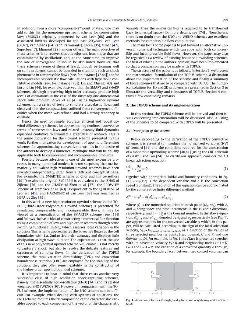
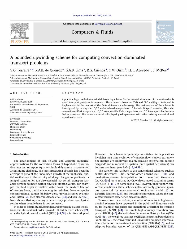
Fig. 1. Advection velocities through f and g faces, and neighboring nodes of thesefaces.

V.G. Ferreira et al. / Computers & Fluids 57 (2012) 208–224 209

In addition, from a more ‘‘compressible’’ point of view, one mayadd to this list the monotone upstream scheme for conservationlaws (MUSCL) originally pioneered by van Leer [68] and theassociated limiters developed for the past 20 years: van Leer[66,67], van Albada [64] (and its variants), Koren [35], Osher [47],Superbee [7], Minmod [28], among others. The main objective ofthese schemes is to recover smooth solutions from those that arecontaminated by oscillations and, at the same time, to improvethe rate of convergence. It should be also noted, however, thatthese schemes (some of them at least), though performing wellon some problems, cannot be bounded in situations such as shockphenomena in compressible flows (see, for instance [37,44]) and/orincompressible viscoelastic flow calculations with hyperbolic con-stitutive models (see, for instance [73]). Lin and Chieng [43] andLin and Lin [44], for example, observed that the SMART and SHARPschemes, although preserving high-order accuracy, produce highlevels of oscillations in the case of the unsteady one-dimensionalshock tube problem; Alves et al. [4], using high-order upwindschemes, ran a series of tests to simulate viscoelastic flows andobserved that the computations suffered from convergence diffi-culties when the mesh was refined, and had a strong tendency tooscillate.

Hence, the need for simple, accurate, efficient and robust up-wind differencing schemes for approximating nonlinear convectiveterms of conservation laws and related unsteady fluid dynamicsequations continues to stimulate a great deal of research. This isthe prime motivation for the upwind scheme presented in thiswork. Further motivation for development of upwind differencingschemes for approximating convective terms lies in the desire ofthe authors to develop a numerical technique that will be equallyapplicable both to compressible and incompressible problems.

Possibly because advection is one of the most expensive pro-cesses in many numerical models, it is not surprising that mathe-matically equivalent high resolution upwind schemes have beeninvented independently, often from a different conceptual basis.For example, the SMARTER scheme of Choi and his co-authors[19] (see also the original Ref. [55]) is equivalent to the ISNAS ofZijlema [76] and the CHARM of Zhou et al. [77]; the CROWLEYscheme of Tremback et al. [63] is equivalent to the QUICKEST ofLeonard [41]; and HARMONIC of van Leer [68] was renamed asHLPA by Zhu [79].

In this work, a new high resolution upwind scheme, called TO-PUS (Third-Order Polynomial Upwind Scheme) is presented forsimulating compressible and incompressible flows; it may beviewed as a generalization of the SMARTER scheme (see [19])and follows the basic idea of constructing a numerical flux functionusing a combination of low and high order schemes through someswitching function (limiter), which assesses local variation in thesolution. This scheme approximates the advective fluxes at the cellboundaries with 1st, 2nd or 3rd order accuracy and displays littledissipation at high wave number. The expectation is that the useof this new polynomial upwind scheme will enable us not merelyto capture a shock, but also to resolve the delicate features andstructures of complex flows. In the derivation of the TOPUSscheme, the total variation diminishing (TVD) and convectionboundedness criterion (CBC) are employed for the stability of thesolution; they also offer some flexibility in the construction ofthe higher-order upwind bounded schemes.

It is important to bear in mind that there exists another verysuccessful class of high resolution shock-capturing schemes,namely, the essentially non-oscillatory (ENO) [34] (and its relatedweighted ENO (WENO) [9]). However, in comparison with the TO-PUS scheme, the implementation of the ENO scheme can be diffi-cult. For example, when dealing with systems of equations, theENO scheme requires the decomposition of the characteristic vari-ables applied to each component of the vector of the characteristic

variable; then the numerical flux is required to be transformedback to physical space (for more details, see [74]). Nonetheless,there is no doubt that the ENO and WENO schemes are excellentmethods for compressible flow computation.

The main focus of the paper is to put forward an alternative uni-versal numerical technique which can cope with both compress-ible and incompressible fluid flows. However, the paper may alsobe regarded as a review of existing bounded upwinding schemes,the best of which (in the authors’ opinion) have been implementedso that a comparison may be made with TOPUS.

The structure of the paper is as follows. In Section 2, we presentthe mathematical formulation of the TOPUS scheme, a discussionabout the implementation of the scheme and finally a summaryof those schemes that are to be compared with TOPUS. The numer-ical solutions for 1D and 2D problems are presented in Section 3 toillustrate the versatility and robustness of TOPUS. Section 4 con-tains a few concluding remarks.

2. The TOPUS scheme and its implementation

In this section, the TOPUS scheme will be derived and then is-sues concerning implementation will be discussed. Also, a listingof the schemes to be compared with TOPUS will be presented.

2.1. Description of the scheme

Before proceeding to the derivation of the TOPUS convectivescheme, it is essential to introduce the normalized variables (NV)of Leonard [41] and the conditions required for the constructionof a monotonic upwinding scheme [40,41] (using the CBC criterionof Gaskell and Lau [24]). To clarify our approach, consider the 1Dlinear advection equation

@/@tþ a

@/@x¼ 0; ð1Þ

together with appropriate initial and boundary conditions. In Eq.(1), / = /(x, t) is the dependent variable and a is the convectionspeed (constant). The solution of this equation can be approximatedby the conservative finite difference method

/nþ1i ¼ /n

i � h /niþ1=2 � /n

i�1=2

� �; ð2Þ

where /ni is the numerical solution at mesh point (idx, ndt), with dx

and dt being space and time increments in the x- and t-directions,respectively, and h ¼ a dt

dxis the Courant number. In the above equa-

tion, /niþ1=2 and /n

i�1=2, denoted by /f and /g respectively (see Fig. 1),are approximations for the convected variable / which, in this pa-per, will be calculated, according to the sign of the local advectionvelocity, V(�) = V(through a control surface), as a function of the values atthree selected neighboring points (two upwind, U and R, and onedownwind D). For example, in Fig. 1 the f face is presented togetherwith its advection velocity Vf > 0 and neighboring nodes i + 1 = D,i = U and i � 1 = R. The variation of a convected quantity / through,for example, the boundary face f between two control volumes can

210 V.G. Ferreira et al. / Computers & Fluids 57 (2012) 208–224

be represented by a functional relationship linking values /D,/U and/R, which represent, respectively, the Downstream, the Upstreamand the Remote-upstream locations with respect to the advectionvelocity Vf at this face. The neighbors of the g face can be similarlyclassified. If this functional relationship, involving these threeneighboring positions, is prescribed, then the value of the interfaceconvected variable can be determined. To this end, the originalvariable / is transformed into the NV of Leonard [41] by

/̂ðx; tÞ ¼ /ðx; tÞ � /nR

/nD � /n

R

: ð3Þ

The advantage of this normalization is that the interface value /̂f

depends on /̂nU and h only, since /̂n

D ¼ 1 and /̂nR ¼ 0. From now on,

the superscript n will be omitted for simplicity. The CBC is acondition for achieving computed boundedness if only three neigh-boring values are used to approximate the interface numerical con-vected variables. According to Leonard [40,41], a bounded highresolution second and/or third order accurate scheme (in general,nonlinear) within the CBC region must pass through points O(0,0),Q(0.5,0.75), P(1,1) and with inclination of 0.75 at Q. Passing throughQ will provide second order accuracy and passing through Q with aslope of 0.75 will give third order accuracy.

The TOPUS scheme is derived by assuming that the NV at thecell interface f ; /̂f , are related to /̂U by a fourth degree polynomialfunction for 0 < /̂U < 1, and a linear function (the FOU scheme) for/̂U 6 0 and /̂U P 1. The four conditions of Leonard presentedabove, plus a free condition, are imposed to obtain

/̂f ¼a/̂4

U þ ð�2aþ 1Þ/̂3U þ 5a�10

4

� �/̂2

U þ �aþ104

� �/̂U ; /̂U 2 ð0;1Þ;

/̂U ; /̂U R ð0;1Þ;

(ð4Þ

where a is an adjustable constant in the interval [ � 2,2]. If a = 0,then TOPUS falls into the CBC region of Gaskell and Lau [24] andcorresponds to the SMARTER scheme of Choi and co-authors [19](see also Waterson and Deconinck [71]). By imposing an inclinationof 1 at point P (i.e. a continuously differentiable function at P), oneobtains a = 2. Fig. 2 depicts the TOPUS scheme for the case a = 2,where one can see that it is entirely contained within the TVD re-gion of Harten [29]. Other values of a ensure that TOPUS falls withinthe CBC region. In practice, it is necessary to be careful. For incom-pressible flows, it can be chosen from [�2,2] and boundedness willbe ensured; a good choice is a = 0 or a = 2. For compressible flows,one must set a = 2 to guarantee the TVD criterion.

0 0.2 0.4 0.6 0.8 1 1.20

0.2

0.4

0.6

0.8

1

1.2 TOPUSQ=(0.5,0.75)TVD region

Fig. 2. TOPUS with a = 2 on TVD region.

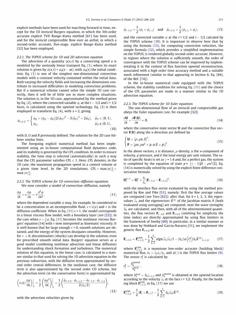
Let rf be a local shock sensor satisfying Sweby’s monotonicitypreservation condition when rf tends to zero. Then the correspond-ing flux limiter w = w(rf) for the TOPUS scheme when a = 2 is de-duced as follows. The variable rf is the ratio of upstream todownstream (consecutive) gradients

rf ¼@/@x

� �f

@/@x

� �g

; ð5Þ

which, for uniform meshes, can be rewritten as

rf ¼/U � /R

/D � /U; ð6Þ

and, in terms of the NV, expressed as

rf ¼/̂U

1� /̂U

: ð7Þ

Consider the general approximation (FOU scheme plus an anti-diffusive term) to the convected variable at the f face

/̂f ¼ /̂U þ12

wðrf Þð1� /̂UÞ: ð8Þ

From Eq. (4), with a = 2, Eqs. (7) and (8), one determines w(rf) as

wðrf Þ ¼ðjrf j þ rf Þ½3rf þ 1�ð1þ jrf jÞ3

: ð9Þ

Fig. 3 displays the TOPUS flux limiter (9) in the rf � w(rf) plane. Itcan be seen that the TOPUS flux limiter is a smooth function of rf

(>0) (see Zijlema [76] and Piperno et al. [49]), so there would appearto be a real possibility that it might perform better than other wellrecognized TVD schemes.

It is important to recognize that the TOPUS upwind schemedeveloped here, for calculating flux derivatives, is derived from1D theory; and in multidimensional cases, it has to be applied (fol-lowing Zhang and Jackson [75]) to each of the coordinate directionsseparately.

2.2. Implementation issues

In this subsection, we show how TOPUS (and other upwindingschemes) may be incorporated into the discretized form of a num-ber of model equations. In addition, a brief discussion concerningthe stability of the computations and the choice of the CFL param-eter is provided. In all calculations, for simplicity, first order

0 0.5 1 1.5 2 2.5 3 3.5 40

0.5

1

1.5

2

2.5TOPUSP=(1,1)TVD region

Fig. 3. Flux limiter w(rf) for the TOPUS with a = 2 on TVD region.

V.G. Ferreira et al. / Computers & Fluids 57 (2012) 208–224 211

explicit methods have been used for marching forward in time, ex-cept for the 1D inviscid Burgers equation, in which the 3th-orderaccurate explicit TVD Runge–Kutta method [61] has been used,and for the inviscid compressible flow over an airfoil, in which asecond-order accurate, five-stage, explicit Runge–Kutta method[32] has been employed.

2.2.1. The TOPUS scheme for 1D and 2D advection equationThe advection of a quantity /(x, t) by a convecting speed a is

modeled by the unsteady linear transport Eq. (1), where its exactsolution is given by /(x, t) = /0(x � at), with /0(x) the initial condi-tion. Eq. (1) is one of the simplest one-dimensional convectionmodels with a constant velocity contained within the initial data.Both varying the velocity fields and increasing the dimensions con-tribute to increased difficulties in modeling convection problems.But if a numerical scheme cannot solve the simple 1D case cor-rectly, then it will be of little use in more complex situations.The solution is, in the 1D case, approximated by the method givenby Eq. (2), where the convected variable /, at the i � 1/2 and i + 1/2faces, is calculated using the upwind technology. Eq. (3) is thenemployed to transform Eq. (4), with a = 2, giving

/i�1=2 ¼/R þ ð/D � /RÞ½2ð/̂UÞ4 � 3ð/̂UÞ3 þ 2/̂U �; /̂U 2 ð0;1Þ;/U ; /̂U R ð0;1Þ;

(ð10Þ

with D, U and R previously defined. The solution for the 2D case fol-lows similar lines.

The foregoing explicit numerical method has been imple-mented using an in-house computational fluid dynamics code,and its stability is governed by the CFL condition. In order to ensurestability, the time step is selected (automatically) in such a waythat the CFL parameter satisfies CFL 6 1. Here, CFL denotes, in the1D case, the maximum propagation speed in a control volume ata given time level. In the 2D simulations, CFL ¼ max juj dt

dxþ

max jv j dtdx

.

2.2.2. The TOPUS scheme for 1D convection–diffusion equationsWe now consider a model of convection–diffusion, namely

@/@tþ e

@/@x¼ m

@2/@x2 ; ð11Þ

where the dependent variable / may, for example, be considered tobe a concentration in an incompressible fluid, e = e(/) and m is thediffusion coefficient. When in Eq. (11) e = 1, the model correspondsto a linear viscous flow model, with a boundary layer (see [22]). Inthe case when e ¼ 1

2 /, Eq. (11) becomes the nonlinear viscous Bur-gers’ equation [14] with m now interpreted as kinematic viscosity. Itis well known that for large enough m > 0, smooth solutions are ob-tained, and the energy of the system dissipates smoothly. However,for m ? 0, discontinuities (shocks) can develop in the solution, evenfor prescribed smooth initial data. Burgers’ equation serves as agood model (combining nonlinear advection and linear diffusion)for understanding shock formation and turbulence. The numericalsolution of this equation, in the linear case, is calculated in a man-ner similar to that used for solving the 1D advection equation in theprevious subsection, with the diffusive term approximated by sec-ond order central differences. In the nonlinear case, the diffusiveterm is also approximated by the second order CD scheme, butthe advection term (in the conservative form) is approximated by

eð/Þ @/@x

� �����i

¼ 12

@/2

@x

!�����i

¼ 12

�/iþ1=2 � /iþ1=2 � �/i�1=2 � /i�1=2

2ðdx=2Þ

!;

ð12Þ

with the advection velocities given by

�/i�1=2 ¼12ð/i þ /i�1Þ and �/iþ1=2 ¼

12ð/iþ1 þ /iÞ; ð13Þ

and the convected variable / at the i + 1/2 and i � 1/2 calculed bythe TOPUS scheme (10). It is important to observe here that byusing the formula (13), for computing convection velocities, thesimple formula (12), which provides a simplified implementationon the TOPUS, is rendered globally second-order accurate. However,in regions where the solution is sufficiently smooth, the order ofconvergence with the TOPUS scheme can be improved by implem-entating it in the context of flux function upwind reconstruction,associated with a high order time accuracy method and a suitablemesh refinement (similar to that appearing in Section 6, Eq. (84),of the Ref. [74]).

In the in-house numerical code equipped with the TOPUSscheme, the stability condition for solving Eq. (11) and the choiceof the CFL parameter are made in a manner similar to the 1Dadvection equation.

2.2.3. The TOPUS scheme for 1D Euler equationsThe one-dimensional flow of an inviscid and compressible gas

obeys the Euler equations (see, for example [32])

@U@tþ @FðUÞ

@x¼ 0; ð14Þ

where the conservative state vector U and the convective flux vec-tor F(U) along the x-direction are defined by

U ¼ ½q;qu; E�T ;F ¼ ½qu;qu2 þ p;uðEþ pÞ�T :

(ð15Þ

In the above vectors, x is distance, q density, u the x-component ofvelocity, p pressure, and E the total energy per unit volume. The ra-tio of specific heats is set as c = 1.4 and, for a perfect gas, the systemis completed by the equation of state p = (c � 1)[E � qu2/2]. Eq.(14) is numerically solved by using the explicit finite difference con-servative formula

Unþ1i ¼ Un

i þdt

dx½Fi�1=2 � Fiþ1=2�n; ð16Þ

with the interface flux vector evaluated by using the method pro-posed by Roe and Pike [51], namely: first the Roe average valuesare computed (see Toro [62]); after that, for k = 1, 2, 3, the eigen-values ekk and the eigenvectors eK ðkÞ of the Jacobian matrix bA (bothevaluated using averaging) are computed; next the wave strengthseak are calculated; and then, with all of the aforementioned quanti-ties, the flux vectors Fi�1/2 and Fi+1/2 (omitting for simplicity thetime index) are directly approximated by using flux limiters inthe framework of Sweby [60]. In particular, in a similar manner aswas done by Hubbard and Garcia-Navarro [31], we implement thegeneric flux Fi+1/2 as

Fiþ1=2 ¼ FLOWiþ1=2 þ

12

X3

k¼1

signð~kkÞ~kkð1� jhkjÞw rkf

� �~akeK ðkÞjiþ1=2; ð17Þ

where FLOWiþ1=2 is a monotone low-order accurate (building block)

numerical flux, hk ¼ ~kkdt=dx, and w(�) is the TOPUS flux limiter (9).The sensor rk

f is calculated by

rkf ¼

~aupwindk

~alocalk

; ð18Þ

where ~alocalk ¼ ~akjiþ1=2 and ~aupwind

k is obtained at the upwind locationaccording to the velocity ~kk at the face i + 1/2. Finally, for the build-ing block FLOW

iþ1=2 in Eq. (17) we use

FLOWiþ1=2 ¼

12ðFi þ Fiþ1Þ �

12

X3

k¼1

~akj~kkjeK ðkÞ: ð19Þ

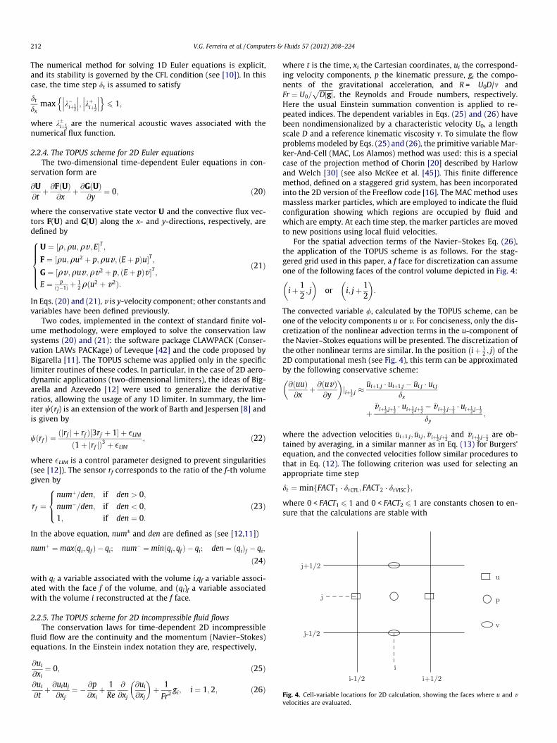
Fig. 4. Cell-variable locations for 2D calculation, showing the faces where u and v

212 V.G. Ferreira et al. / Computers & Fluids 57 (2012) 208–224

The numerical method for solving 1D Euler equations is explicit,and its stability is governed by the CFL condition (see [10]). In thiscase, the time step dt is assumed to satisfy

dt

dxmax k�iþ1

2

��� ���; kþiþ12

��� ���n o6 1;

where k�iþ12

are the numerical acoustic waves associated with thenumerical flux function.

2.2.4. The TOPUS scheme for 2D Euler equationsThe two-dimensional time-dependent Euler equations in con-

servation form are

@U@tþ @FðUÞ

@xþ @GðUÞ

@y¼ 0; ð20Þ

where the conservative state vector U and the convective flux vec-tors F(U) and G(U) along the x- and y-directions, respectively, aredefined by

U ¼ ½q;qu;qv ; E�T ;F ¼ ½qu;qu2 þ p;quv; ðEþ pÞu�T ;G ¼ ½qv ;quv;qv2 þ p; ðEþ pÞv �T ;E ¼ p

ðc�1Þ þ 12 qðu2 þ v2Þ:

8>>>><>>>>: ð21Þ

In Eqs. (20) and (21), v is y-velocity component; other constants andvariables have been defined previously.

Two codes, implemented in the context of standard finite vol-ume methodology, were employed to solve the conservation lawsystems (20) and (21): the software package CLAWPACK (Conser-vation LAWs PACKage) of Leveque [42] and the code proposed byBigarella [11]. The TOPUS scheme was applied only in the specificlimiter routines of these codes. In particular, in the case of 2D aero-dynamic applications (two-dimensional limiters), the ideas of Big-arella and Azevedo [12] were used to generalize the derivativeratios, allowing the usage of any 1D limiter. In summary, the lim-iter w(rf) is an extension of the work of Barth and Jespersen [8] andis given by

wðrf Þ ¼ðjrf j þ rf Þ½3rf þ 1� þ �LIM

ð1þ jrf jÞ3 þ �LIM

; ð22Þ

where �LIM is a control parameter designed to prevent singularities(see [12]). The sensor rf corresponds to the ratio of the f-th volumegiven by

rf ¼numþ=den; if den > 0;num�=den; if den < 0;1; if den ¼ 0:

8><>: ð23Þ

In the above equation, num± and den are defined as (see [12,11])

numþ ¼ maxðqi; qf Þ � qi; num� ¼ minðqi; qf Þ � qi; den ¼ ðqiÞf � qi;

ð24Þ

with qi a variable associated with the volume i,qf a variable associ-ated with the face f of the volume, and (qi)f a variable associatedwith the volume i reconstructed at the f face.

2.2.5. The TOPUS scheme for 2D incompressible fluid flowsThe conservation laws for time-dependent 2D incompressible

fluid flow are the continuity and the momentum (Navier–Stokes)equations. In the Einstein index notation they are, respectively,

@ui

@xi¼ 0; ð25Þ

@ui

@tþ @uiuj

@xj¼ � @p

@xiþ 1

Re@

@xj

@ui

@xj

� �þ 1

Fr2 gi; i ¼ 1;2; ð26Þ

where t is the time, xi the Cartesian coordinates, ui the correspond-ing velocity components, p the kinematic pressure, gi the compo-nents of the gravitational acceleration, and R = U0D/m andFr ¼ U0=

ffiffiffiffiffiffiffiffiffiDjgj

p, the Reynolds and Froude numbers, respectively.

Here the usual Einstein summation convention is applied to re-peated indices. The dependent variables in Eqs. (25) and (26) havebeen nondimensionalized by a characteristic velocity U0, a lengthscale D and a reference kinematic viscosity m. To simulate the flowproblems modeled by Eqs. (25) and (26), the primitive variable Mar-ker-And-Cell (MAC, Los Alamos) method was used: this is a specialcase of the projection method of Chorin [20] described by Harlowand Welch [30] (see also McKee et al. [45]). This finite differencemethod, defined on a staggered grid system, has been incorporatedinto the 2D version of the Freeflow code [16]. The MAC method usesmassless marker particles, which are employed to indicate the fluidconfiguration showing which regions are occupied by fluid andwhich are empty. At each time step, the marker particles are movedto new positions using local fluid velocities.

For the spatial advection terms of the Navier–Stokes Eq. (26),the application of the TOPUS scheme is as follows. For the stag-gered grid used in this paper, a f face for discretization can assumeone of the following faces of the control volume depicted in Fig. 4:

iþ 12; j

� �or i; jþ 1

2

� �:

The convected variable /, calculated by the TOPUS scheme, can beone of the velocity components u or v. For conciseness, only the dis-cretization of the nonlinear advection terms in the u-component ofthe Navier–Stokes equations will be presented. The discretization ofthe other nonlinear terms are similar. In the position iþ 1

2 ; j� �

of the2D computational mesh (see Fig. 4), this term can be approximatedby the following conservative scheme:

@ðuuÞ@xþ @ðuvÞ

@y

� �jiþ1

2;j�

�uiþ1;j � uiþ1;j � �ui;j � ui;j

dx

þ�v iþ1

2;jþ12� uiþ1

2;jþ12� �v iþ1

2;j�12� uiþ1

2;j�12

dy;

where the advection velocities �uiþ1;j; �ui;j; �v iþ12;jþ

12

and �v iþ12;j�

12

are ob-tained by averaging, in a similar manner as in Eq. (13) for Burgers’equation, and the convected velocities follow similar procedures tothat in Eq. (12). The following criterion was used for selecting anappropriate time step

dt ¼minfFACT1 � dt CFL; FACT2 � dt VISCg;

where 0 < FACT1 6 1 and 0 < FACT2 6 1 are constants chosen to en-sure that the calculations are stable with

velocities are evaluated.

0

0.2

0.4

0.6

0.8

1

1.2

100 100.2 100.4 100.6 100.8 101

ExactADBQUICKEST

0

0.2

0.4

0.6

0.8

1

1.2

100 100.2 100.4 100.6 100.8 101

ExactSMART

0

0.2

0.4

0.6

0.8

1

1.2

100 100.2 100.4 100.6 100.8 101

ExactWACEB

0

0.2

0.4

0.6

0.8

1

1.2

100 100.2 100.4 100.6 100.8 101

ExactVONOS

0

0.2

0.4

0.6

0.8

1

1.2

100 100.2 100.4 100.6 100.8 101

Exactvan Albada

0

0.2

0.4

0.6

0.8

1

1.2

100 100.2 100.4 100.6 100.8 101

ExactTOPUS

Fig. 5. Test case 1: numerical (blue symbol) and exact (red line) of the unsteady linear advection equation. (For interpretation of the references to colour in this figure legend,the reader is referred to the web version of this article.)

Table 1Computing time per mesh point per iteration and normalized costs by the unit cost ofthe WACEB scheme (cheapest).

Scheme Unit cost (ls) Normalized costs

ADBQUICKEST 0.35 1.13SMART 2.13 6.87WACEB 0.31 1.00VONOS 1.45 4.68van Albada 0.33 1.06TOPUS 0.32 1.03

V.G. Ferreira et al. / Computers & Fluids 57 (2012) 208–224 213

dt CFL ¼maxdx

juj ;dy

jv j

�and dt VISC ¼

Re2

d2xd

2y

d2x þ d2

y

:

2.2.6. Popular upwinding schemesIn this subsection, we list the schemes that are to be compared

with TOPUS. We also detail flux limiter functions.Non-normalizedvariable schemes:

� SMART [24]:

/f ¼

/U if /̂U R ½0;1�;

10/U � 9/R if 0 6 /̂U < 3=74;18 ð3/D þ 6/U � /RÞ if 3=74 6 /̂U < 5=6;

/D if 5=6 6 /̂U 6 1;

8>>>>><>>>>>:

� VONOS [65]:

/f ¼

/U if /̂U R ½0;1�;

10/U � 9/R if 0 6 /̂U < 3=74;38 /D þ 3

4 /U � 18 /R if 3=74 6 /̂U < 1=2;

1:5/U � 0:5/R if 1=2 6 /̂U < 2=3;

/D if 2=3 6 /̂U 6 1;

8>>>>>>>>><>>>>>>>>>:

� WACEB [57]:

/f ¼

/U if /̂U R ½0;1�;

2/U � /R if 0 6 /̂U < 3=10;34 /U � 3

8 /D � 18 /R if 3=10 6 /̂U < 5=6;

/D if 5=6 6 /̂U 6 1;

8>>>>><>>>>>:

Table 2Errors and computed convergence rates for 2D advection equation, with CFL = 0.5 at time t = 2. Here, ADB refers to ADBQUICKEST.

Scheme Mesh L1-error Convergence rate L2-error Convergence rate

ADB 16 � 16 7.40e�3 – 3.00e�2 –32 � 32 1.81e�3 2.0 1.09e�2 1.564 � 64 4.74e�4 1.9 4.14e�3 1.4128 � 128 1.20e�4 2.0 1.50e�3 1.5256 � 256 3.03e�5 2.0 5.37e�4 1.5

Superbee 16 � 16 8.94e�3 – 3.63e�2 –32 � 32 1.87e�3 2.3 1.15e�2 1.764 � 64 4.60e�4 2.0 4.05e�3 1.5128 � 128 1.19e�4 2.0 1.49e�3 1.4256 � 256 3.02e�5 2.0 5.35e�4 1.5

van Leer 16 � 16 6.97e�3 – 2.81e�2 –32 � 32 1.82e�3 1.9 1.09e�2 1.464 � 64 4.74e�4 1.9 4.14e�3 1.4128 � 128 1.20e�4 2.0 1.50e�3 1.5256 � 256 3.03e�5 2.0 5.37e�4 1.5

van Albada 16 � 16 8.85e�3 – 3.61e�2 –32 � 32 4.47e�3 1.0 2.67e�2 0.464 � 64 6.08e�4 2.9 5.29e�3 2.3128 � 128 1.46e�4 2.1 1.82e�3 1.5256 � 256 3.40e�5 2.1 6.02e�4 1.6

TOPUS 16 � 16 1.01e�2 – 4.09e�2 –32 � 32 3.39e�3 1.6 2.02e�2 1.064 � 64 5.63e�4 2.6 4.91e�3 2.0128 � 128 1.34e�4 2.1 1.67e�3 1.6256 � 256 3.20e�5 2.1 5.66e�4 1.6

214 V.G. Ferreira et al. / Computers & Fluids 57 (2012) 208–224

� Superbee [7]:

Table 3Errors a

Sche

van

TOPU

/f ¼

/U if /̂U R ½0;1�;2/U � /R if 0 6 /̂U < 1=3;12 ð/D þ /UÞ if 1=3 6 /̂U < 1=2;32 /U � 1

2 /R if 1=2 6 /̂U < 2=3;

/D if 2=3 6 /̂U 6 1;

8>>>>>>><>>>>>>>:

� CUBISTA [5]:

/f ¼

/U if /̂U R ½0;1�;74 /U � 3

4 /R if 0 6 /̂U < 3=8;38 /D � 3

4 /U � 18 /R if 3=8 6 /̂U < 3=4;

34 /D þ 1

4 /U if 3=4 6 /̂U 6 1;

8>>>>><>>>>>:

� ADBQUICKEST [23]:

/f ¼

/U if /̂U R ½0;1�;ð2� hÞ/U � ð1� hÞ/R if 0 6 /̂U < a;

aD/D þ aU/U � aR/RÞ if a 6 /̂U 6 b;

ð1� hÞ/D þ h/U if b < /̂U < 1;

8>>>><>>>>:

with

nd computed convergence rates for 1D inviscid Burgers’ equation, with u0(x) = 1 + 0.5sin(p

me Mesh L1-error Convergen

Albada 20 2.880e�02 –40 7.872e�03 1.880 1.700e�03 2.2

160 5.350e�04 1.7320 1.248e�04 2.1

S 20 1.825e�02 –40 3.551e�03 2.380 9.460e�04 1.9

160 1.720e�04 2.4320 3.492e�05 2.3

aD ¼ 16 ð2� 3hþ h2Þ; aU ¼ 1

6 ð5þ 3h� 2h2Þ; aR ¼ 16 ð1� h2Þ;

a ¼ 2� 3hþ h2

7� 9hþ 2h2 ; b ¼ �4þ 3hþ h2

�5þ 3hþ 2h2 :

Flux limiter functions:

� Minmod [28]: w(rf) = minmod (1,rf);

� Superbee [7]: w(rf) = max (0,min (1,2rf), min (2,rf));

� monotonized centered (MC) [67]: w(rf) = max (0,min ((1 + rf)/2,2,2rf));� van Leer [66]: wðrf Þ ¼

rf þ jrf j1þ jrf j

;

� van Albada [64]: wðrf Þ ¼r2

f þ rf

1þ r2f

;

� ADBQUICKEST [23]:

wðrf Þ ¼max 0;min 2rf ;2þh2�3hþð1�h2Þrf

3�3h ;2n on o

:

3. Numerical experiments

In order to demonstrate the behavior, validity, flexibility,robustness and practicality of the TOPUS scheme, we have per-formed numerous simulations based on benchmark test cases,including 2D compressible/incompressible flows. Comparisonsare made both with exact solutions and with well-recognized

x), �1 < x < 1 at time t = 0.12.

ce rate L1-error Convergence rate

7.017e�02 –2.462e�02 1.59.010e�03 1.42.862e�03 1.68.219e�04 1.8

5.250e�02 –1.530e�02 1.74.630e�03 1.71.150e�03 2.03.303e�04 1.8

0

0.1

0.2

0.3

0.4

0.5

0.6

-1.5 -1 -0.5 0 0.5 1

ExactADBQUICKEST

0

0.1

0.2

0.3

0.4

0.5

0.6

-1.5 -1 -0.5 0 0.5 1

ExactSMART

0

0.1

0.2

0.3

0.4

0.5

0.6

-1.5 -1 -0.5 0 0.5 1

ExactTOPUS

0

0.1

0.2

0.3

0.4

0.5

0.6

-1.5 -1 -0.5 0 0.5 1

ExactVONOS

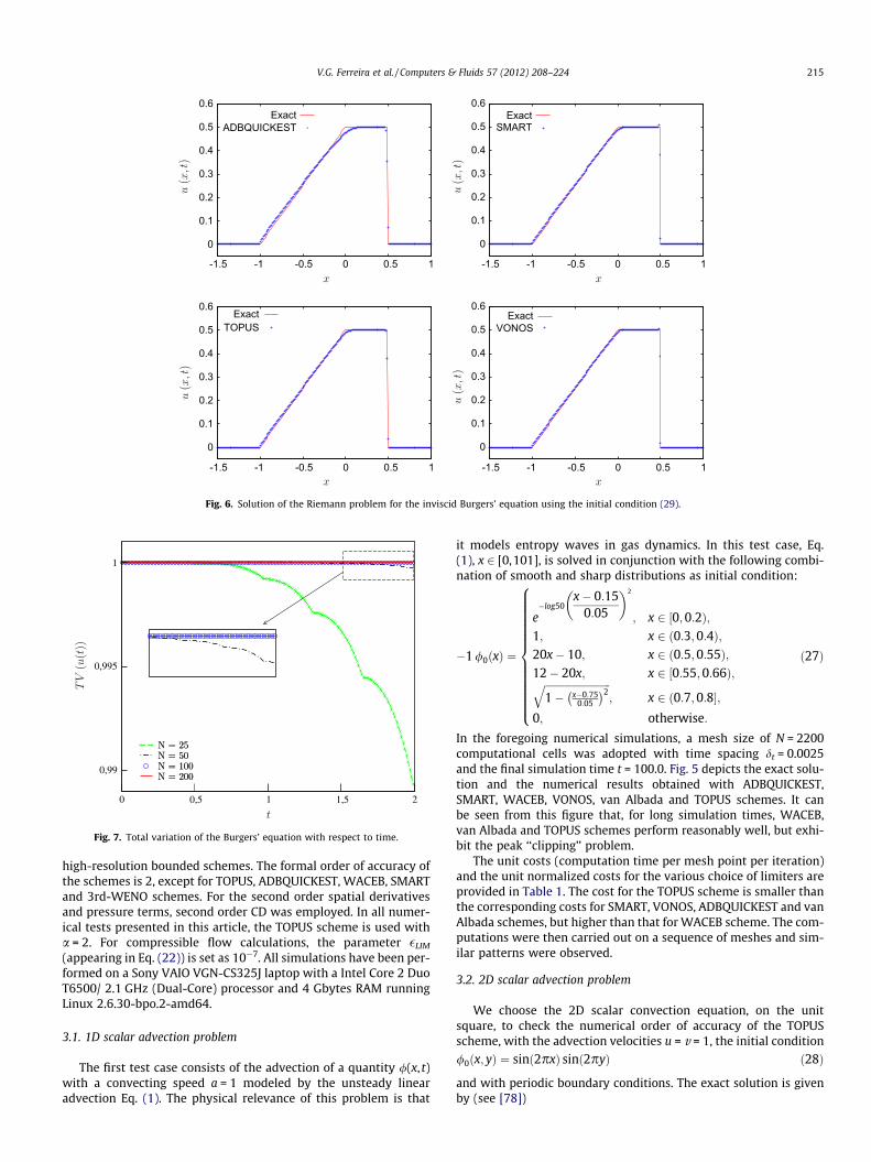
Fig. 6. Solution of the Riemann problem for the inviscid Burgers’ equation using the initial condition (29).

0 0,5 1 1,5 2

0,99

0,995

1

Fig. 7. Total variation of the Burgers’ equation with respect to time.

V.G. Ferreira et al. / Computers & Fluids 57 (2012) 208–224 215

high-resolution bounded schemes. The formal order of accuracy ofthe schemes is 2, except for TOPUS, ADBQUICKEST, WACEB, SMARTand 3rd-WENO schemes. For the second order spatial derivativesand pressure terms, second order CD was employed. In all numer-ical tests presented in this article, the TOPUS scheme is used witha = 2. For compressible flow calculations, the parameter �LIM

(appearing in Eq. (22)) is set as 10�7. All simulations have been per-formed on a Sony VAIO VGN-CS325J laptop with a Intel Core 2 DuoT6500/ 2.1 GHz (Dual-Core) processor and 4 Gbytes RAM runningLinux 2.6.30-bpo.2-amd64.

3.1. 1D scalar advection problem

The first test case consists of the advection of a quantity /(x, t)with a convecting speed a = 1 modeled by the unsteady linearadvection Eq. (1). The physical relevance of this problem is that

it models entropy waves in gas dynamics. In this test case, Eq.(1), x 2 [0,101], is solved in conjunction with the following combi-nation of smooth and sharp distributions as initial condition:

�1 /0ðxÞ ¼

e�log50

x� 0:150:05

� �2

; x 2 ½0;0:2Þ;1; x 2 ð0:3;0:4Þ;20x� 10; x 2 ð0:5;0:55Þ;12� 20x; x 2 ½0:55;0:66Þ;ffiffiffiffiffiffiffiffiffiffiffiffiffiffiffiffiffiffiffiffiffiffiffiffiffiffi

1� x�0:750:05

� �2q

; x 2 ð0:7;0:8�;0; otherwise:

8>>>>>>>>>>>>><>>>>>>>>>>>>>:ð27Þ

In the foregoing numerical simulations, a mesh size of N = 2200computational cells was adopted with time spacing dt = 0.0025and the final simulation time t = 100.0. Fig. 5 depicts the exact solu-tion and the numerical results obtained with ADBQUICKEST,SMART, WACEB, VONOS, van Albada and TOPUS schemes. It canbe seen from this figure that, for long simulation times, WACEB,van Albada and TOPUS schemes perform reasonably well, but exhi-bit the peak ‘‘clipping’’ problem.

The unit costs (computation time per mesh point per iteration)and the unit normalized costs for the various choice of limiters areprovided in Table 1. The cost for the TOPUS scheme is smaller thanthe corresponding costs for SMART, VONOS, ADBQUICKEST and vanAlbada schemes, but higher than that for WACEB scheme. The com-putations were then carried out on a sequence of meshes and sim-ilar patterns were observed.

3.2. 2D scalar advection problem

We choose the 2D scalar convection equation, on the unitsquare, to check the numerical order of accuracy of the TOPUSscheme, with the advection velocities u = v = 1, the initial condition

/0ðx; yÞ ¼ sinð2pxÞ sinð2pyÞ ð28Þ

and with periodic boundary conditions. The exact solution is givenby (see [78])

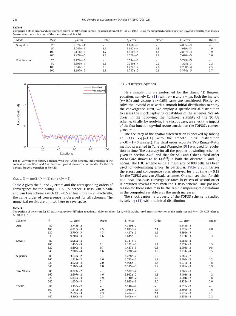
Table 4Comparison of the errors and convergence orders for 1D viscous Burgers’ equation at time 0.25, for dt = 0.001, using the simplified and flux function upwind reconstruction modes.Measured errors as function of the mesh size and Re = 20.

Mode Mesh L1-error Order L2-error Order L1-error Order

Simplified 25 9.374e�4 – 1.696e�3 – 4.035e�3 –50 3.045e�4 1.6 5.012e�4 1.8 1.089e�3 1.9

100 9.111e�5 1.7 1.400e�4 1.8 2.887e�4 1.9200 2.472e�5 1.8 3.700e�5 1.9 7.420e�5 2.0

Flux function 25 2.772e�3 – 3.574e�3 – 5.729e�3 –50 5.595e�4 2.3 7.360e�4 2.3 1.228e�3 2.2

100 9.544e�5 2.6 1.222e�4 2.6 2.238e�4 2.5200 1.397e�5 2.8 1.797e�5 2.8 3.374e�5 2.7

20 40 60 80 100−15

−10

−5

0

Iterations

Log

(Res

idua

l)

SimplifiedFlux function

Fig. 8. Convergence history obtained with the TOPUS scheme, implemented in thecontext of simplified and flux function upwind reconstruction modes, for the 1Dviscous Burgers’ equation at Re = 20.

216 V.G. Ferreira et al. / Computers & Fluids 57 (2012) 208–224

/ðx; y; tÞ ¼ sinð2pðx� tÞÞ sinð2pðy� tÞÞ:

Table 2 gives the L1 and L2 errors and the corresponding orders ofconvergence for the ADBQUICKEST, Superbee, TOPUS, van Albadaand van Leer schemes with CFL = 0.5 at final time t = 2. Practically,the same order of convergence is observed for all schemes. Thenumerical results are omitted here to save space.

Table 5Comparison of the errors for 1D scalar convection–diffusion equation, at different times, foADBQUICKEST.

Scheme N L1-error Order

ADB 80 3.748e�2 –160 6.810e�3 2.5320 2.700e�3 1.3640 9.200e�4 1.6

SMART 80 5.960e�3 –160 1.430e�3 2.1320 8.600e�4 0.7640 2.900e�4 1.6

Superbee 80 3.647e�2 –160 1.212e�2 1.6320 3.020e�3 2.0640 7.500e�4 2.0

van Albada 80 8.023e�2 –160 2.607e�2 1.6320 6.830e�3 1.9640 1.630e�3 2.1

TOPUS 80 5.330e�2 –160 1.319e�2 2.0320 2.690e�3 2.3640 5.300e�4 2.3

3.3. 1D Burgers’ equation

Here simulations are performed for the classic 1D Burgers’equation, namely Eq. (11) with / = u and � ¼ 1

2 u. Both the inviscid(m = 0.0) and viscous (m = 0.05) cases are considered. Firstly, wesolve the inviscid case with a smooth initial distribution to studythe convergence. Next, we employ a specific initial distributionto assess the shock capturing capabilities of the schemes. We ad-dress, in the following, the nonlinear stability of the TOPUSscheme. Finally, by resolving the viscous case, we check the impactof the flux function upwind reconstruction on the TOPUS’s conver-gence rate.

The accuracy of the spatial discretization is checked by solvingEq. (11), x 2 [�1,1], with the smooth initial distributionu(x,0) = 1 + 0.5sin(px). The third order accurate TVD Runge–Kuttamethod presented in Tang and Warnecke [61] was used for evolu-tion in time. The accuracy for all the popular upwinding schemes,given in Section 2.2.6, and that for Shu and Osher’s third-orderWENO are shown to be O(h5/2) in both the discrete L1 and L1norms. The FOU scheme using a mesh size of 800 cells has beenused for determining errors. In particular, Table 3 summarizesthe errors and convergence rates observed for u at time t = 0.12for the TOPUS and van Albada schemes. One can see that, for thisnonlinear test case, convergence rates in excess of second orderis obtained several times with the TOPUS scheme. One possiblereason for these rates may be the rapid dampening of oscillationsin the computed variable u as the mesh increases.

The shock capturing property of the TOPUS scheme is studiedby solving (11) with the initial distribution

r dt = 0.01/N. Measured errors as function of the mesh size and Re = 100. ADB refers to

L2-error Order L1-error Order

4.349e�2 – 5.545e�2 –1.013e�2 2.1 1.379e�2 2.04.497e�3 1.2 6.299e�3 1.11.645e�3 1.5 2.311e�3 1.4

6.731e�3 – 8.284e�3 –2.122e�3 1.7 2.877e�3 1.51.437e�3 0.6 2.005e�3 0.55.220e�4 1.5 7.334e�4 1.5

4.228e�2 – 5.386e�2 –1.793e�2 1.2 2.404e�2 1.24.998e�3 1.8 6.970e�3 1.81.335e�3 1.9 1.888e�3 1.9

9.582e�2 – 1.266e�1 –3.912e�2 1.3 5.401e�2 1.21.140e�2 1.8 1.601e�2 1.82.923e�3 2.0 4.122e�3 2.0

6.248e�2 – 8.073e�2 –1.968e�2 1.7 2.692e�2 1.64.484e�3 2.1 6.278e�3 2.19.608e�4 2.2 1.352e�3 2.2

1

1.5

2

2.5

3

3.5

4

4.5

5

1 1.5 2 2.5 3

ReferenceADBQUICKEST, N = 200ADBQUICKEST, N = 300

1

1.5

2

2.5

3

3.5

4

4.5

5

1 1.5 2 2.5 3

ReferenceLax-Wendroff, N = 200Lax-Wendroff, N = 300

1

1.5

2

2.5

3

3.5

4

4.5

5

1 1.5 2 2.5 3

ReferenceMINMOD, N = 200MINMOD, N = 300

1

1.5

2

2.5

3

3.5

4

4.5

5

1 1.5 2 2.5 3

ReferenceSuperbee, N = 200Superbee, N = 300

1

1.5

2

2.5

3

3.5

4

4.5

5

1 1.5 2 2.5 3

Referencevan Leer, N = 200van Leer, N = 300

1

1.5

2

2.5

3

3.5

4

4.5

5

1 1.5 2 2.5 3

ReferenceTOPUS, N = 200TOPUS, N = 300

Fig. 9. Density distribution for the Shu–Osher shock tube problem using ADBQUICKEST, Lax-Wendroff, Minmod, Superbee, van Leer and TOPUS schemes.

Fig. 10. Geometry of the backward facing step problem, showing a set ofcomputational cells adjacent to the wall.

200 400 600 8002

4

6

8

10

12

14

16Armaly et al. (Num.)Armaly et al. (Exp.)Ku et al.Jiang et al.Williams and Baker 2DWilliams and Baker 3DTOPUSADBQUICKEST

Fig. 11. Comparison between experimental data and numerical results for the sizeof the recirculation region length x1 as a function of the Reynolds number. A close-up of the results are provided in the inset.

V.G. Ferreira et al. / Computers & Fluids 57 (2012) 208–224 217

uðx;0Þ ¼0:0; if x 6 �1;0:5; if � 1 < x < 0;0:0; if x P 0:

8><>: ð29Þ

The exact solution is the rarefaction wave given by Ahmed (see [3]):

uðx; tÞ ¼

0:0; if x 6 �1;xþ1

t ; if � 1 < x 6 t2� 1;

0:5; if t2� 1 < x < t

4 ;

0:0; if x P t4 :

8>>><>>>:

This problem consists of a jump from zero to one at x = � 1/3 whichcreates an expansion fan, while the jump from one to zero at x = 1/3produces a shock wave. The purpose of this test is to check whether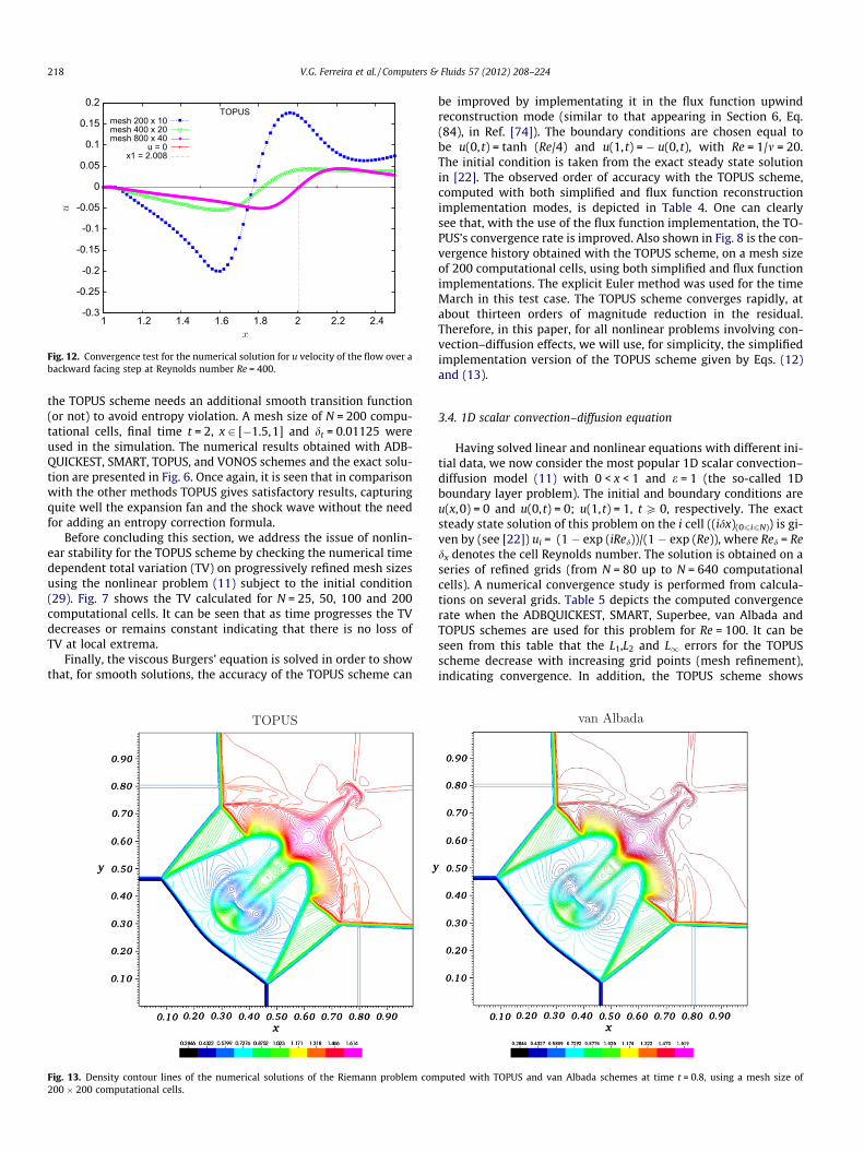

-0.3

-0.25

-0.2

-0.15

-0.1

-0.05

0

0.05

0.1

0.15

0.2

1 1.2 1.4 1.6 1.8 2 2.2 2.4

TOPUSmesh 200 x 10mesh 400 x 20mesh 800 x 40

u = 0x1 = 2.008

Fig. 12. Convergence test for the numerical solution for u velocity of the flow over abackward facing step at Reynolds number Re = 400.

218 V.G. Ferreira et al. / Computers & Fluids 57 (2012) 208–224

the TOPUS scheme needs an additional smooth transition function(or not) to avoid entropy violation. A mesh size of N = 200 compu-tational cells, final time t = 2, x 2 [�1.5,1] and dt = 0.01125 wereused in the simulation. The numerical results obtained with ADB-QUICKEST, SMART, TOPUS, and VONOS schemes and the exact solu-tion are presented in Fig. 6. Once again, it is seen that in comparisonwith the other methods TOPUS gives satisfactory results, capturingquite well the expansion fan and the shock wave without the needfor adding an entropy correction formula.

Before concluding this section, we address the issue of nonlin-ear stability for the TOPUS scheme by checking the numerical timedependent total variation (TV) on progressively refined mesh sizesusing the nonlinear problem (11) subject to the initial condition(29). Fig. 7 shows the TV calculated for N = 25, 50, 100 and 200computational cells. It can be seen that as time progresses the TVdecreases or remains constant indicating that there is no loss ofTV at local extrema.

Finally, the viscous Burgers’ equation is solved in order to showthat, for smooth solutions, the accuracy of the TOPUS scheme can

Fig. 13. Density contour lines of the numerical solutions of the Riemann problem com200 � 200 computational cells.

be improved by implementating it in the flux function upwindreconstruction mode (similar to that appearing in Section 6, Eq.(84), in Ref. [74]). The boundary conditions are chosen equal tobe u(0, t) = tanh (Re/4) and u(1, t) = � u(0, t), with Re = 1/m = 20.The initial condition is taken from the exact steady state solutionin [22]. The observed order of accuracy with the TOPUS scheme,computed with both simplified and flux function reconstructionimplementation modes, is depicted in Table 4. One can clearlysee that, with the use of the flux function implementation, the TO-PUS’s convergence rate is improved. Also shown in Fig. 8 is the con-vergence history obtained with the TOPUS scheme, on a mesh sizeof 200 computational cells, using both simplified and flux functionimplementations. The explicit Euler method was used for the timeMarch in this test case. The TOPUS scheme converges rapidly, atabout thirteen orders of magnitude reduction in the residual.Therefore, in this paper, for all nonlinear problems involving con-vection–diffusion effects, we will use, for simplicity, the simplifiedimplementation version of the TOPUS scheme given by Eqs. (12)and (13).

3.4. 1D scalar convection–diffusion equation

Having solved linear and nonlinear equations with different ini-tial data, we now consider the most popular 1D scalar convection–diffusion model (11) with 0 < x < 1 and e = 1 (the so-called 1Dboundary layer problem). The initial and boundary conditions areu(x,0) = 0 and u(0, t) = 0; u(1, t) = 1, t P 0, respectively. The exactsteady state solution of this problem on the i cell ((idx)(06i6N)) is gi-ven by (see [22]) ui = (1 � exp (iRed))/(1 � exp (Re)), where Red = Redx denotes the cell Reynolds number. The solution is obtained on aseries of refined grids (from N = 80 up to N = 640 computationalcells). A numerical convergence study is performed from calcula-tions on several grids. Table 5 depicts the computed convergencerate when the ADBQUICKEST, SMART, Superbee, van Albada andTOPUS schemes are used for this problem for Re = 100. It can beseen from this table that the L1,L2 and L1 errors for the TOPUSscheme decrease with increasing grid points (mesh refinement),indicating convergence. In addition, the TOPUS scheme shows

puted with TOPUS and van Albada schemes at time t = 0.8, using a mesh size of

0 0,2 0,4 0,6 0,8 10

0,5

1

1,5

2ReferenceTOPUSvan Albada

0 0,2 0,4 0,6 0,8 1-2

-1

0

1

2ReferenceTOPUSvan Albada

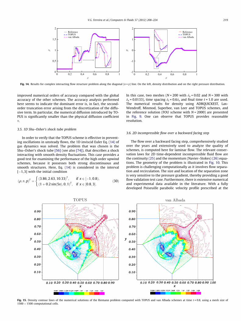
Fig. 14. Results for complex interacting flow structure problem along the diagonal (x = y) line. On the left, density distribution and on the right pressure distribution.

V.G. Ferreira et al. / Computers & Fluids 57 (2012) 208–224 219

improved numerical orders of accuracy compared with the globalaccuracy of the other schemes. The accuracy analysis performedhere seems to indicate the dominant error is, in fact, the second-order truncation error arising from the discretization of the diffu-sive term. In particular, the numerical diffusion introduced by TO-PUS is significantly smaller than the physical diffusion coefficientm.

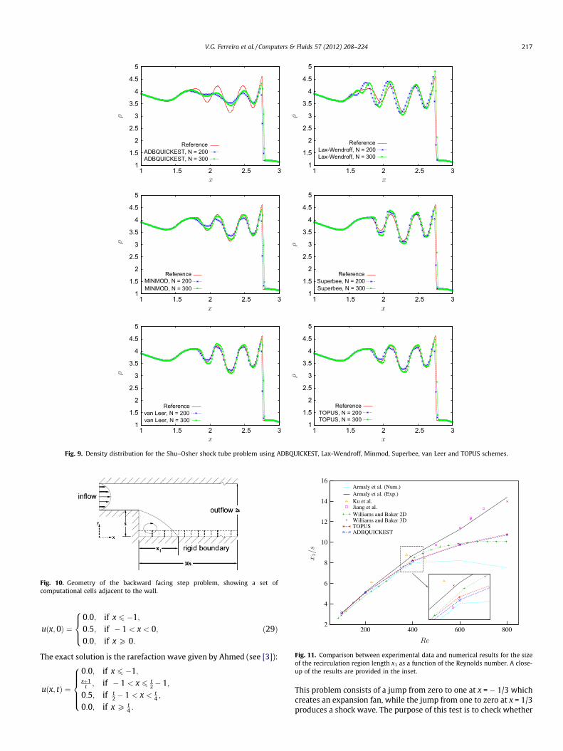
3.5. 1D Shu–Osher’s shock tube problem

In order to verify that the TOPUS scheme is effective in prevent-ing oscillations in unsteady flows, the 1D inviscid Euler Eq. (14) ofgas dynamics was solved. The problem that was chosen is theShu–Osher’s shock tube [56] (see also [74]), that describes a shockinteracting with smooth density fluctuations. This case provides agood test for examining the performance of the high order upwindschemes, because it possesses both strong discontinuous andsmooth structures. Here, Eq. (14) is considered in the interval[�1,3] with the initial condition

ðq; t; pÞT ¼ ð3:86;2:63;10:33ÞT ; if x 2 ½�1;0:8Þ;ð1þ 0:2 sinð5xÞ;0;1ÞT ; if x 2 ½0:8;3�:

(ð30Þ

Fig. 15. Density contour lines of the numerical solutions of the Riemann problem com1500 � 1500 computational cells.

In this case, two meshes (N = 200 with dx = 0.02 and N = 300 withdx = 0.0133), time spacing dt = 0.6dx and final time t = 1.0 are used.The numerical results for density using ADBQUICKEST, Lax-Wendroff, Minmod, Superbee, van Leer and TOPUS schemes, andthe reference solution (FOU scheme with N = 2000) are presentedin Fig. 9. One can observe that TOPUS provides reasonableresolution.

3.6. 2D incompressible flow over a backward facing step

The flow over a backward facing step, comprehensively studiedover the years and extensively used to analyze the quality ofschemes, is computed here for laminar flow. The relevant conser-vation laws for 2D time-dependent incompressible fluid flow arethe continuity (25) and the momentum (Navier–Stokes) (26) equa-tions. The geometry of the problem is illustrated in Fig. 10. Thisproblem is challenging computationally as it involves flow separa-tion and recirculation. The size and location of the separation zoneis very sensitive to the pressure gradient, thereby providing a goodflow validation test case. Furthermore, there is extensive numericaland experimental data available in the literature. With a fullydeveloped Poiseuille parabolic velocity profile prescribed at the

puted with TOPUS and van Albada schemes at time t = 0.8, using a mesh size of

Iterations

Log

(Res

idua

l)

0 20000 40000

-6

-4

-2

0

2

van AlbadaT OPUS

Fig. 16. Convergence histories with van Albada and TOPUS schemes for a NACA0012 airfoil at M1 = 0.85 and a = 1�.

X/C

Cp

0 0.25 0.5 0.75 1

-1

-0.5

0

0.5

1

van AlbadaTOPUS

X/C

Cp

0.7 0.8 0.9

-1

-0.5

0

van AlbadaTOPUS

Fig. 17. Comparison between numerical results obtained with TOPUS and vanAlbada limiters for the pressure coefficient distributions for a NACA 0012 airfoil atM1 = 0.85 and a = 1�.

220 V.G. Ferreira et al. / Computers & Fluids 57 (2012) 208–224

inlet section, we simulated numerically this fluid flow problem fora wide range of Reynolds numbers. These were based on the max-imum velocity U0 = Umax = 1 m/s at the entrance section and theheight of the step s (s = D = 0.1 m). The dimension of the computa-tional domain is 4.0 m � 0.2 m and the total time of simulation is100 seconds. A mesh size of 800 � 40 computational cells has beenused in the simulations.

Fig. 11 graphically displays the evolution of reattachmentlengths x1, normalized by the step height s. With Reynolds num-bers from 100 up to 800, we have the following data: 2D numericalresults of Armaly et al. [6] and Willians and Baker [72]; 3D numer-ical results of Willians and Baker [72], Ku et al. [36], Jiang et al. [34]and the experimental data of Armaly et al. [6]. We also have calcu-lations using TOPUS and ADBQUICKEST schemes (no significantimprovement was observed in the results obtained using the otherschemes). The numerical results using ADBQUICKEST, for0 < Re < 400, show good agreement with the 2D results of Williansand Baker [72]; they would appear, however, to diverge from thedata of Armaly et al. [6] and the 3D calculations. For Re P 400,the numerical results of both TOPUS and ADBQUICKEST give pooragreement with 3D data; this may be explained by 3D effectsand, possibly, the turbulence transition in this high Reynolds num-ber problem, as postulated by Ghia et al. [26]. This figure alsoshows a close-up, where it can be seen that the results obtainedwith the TOPUS scheme are marginally better than those obtainedusing the ADBQUICKEST scheme.

In addition, a convergence test of the numerical solution for(streamwise) velocity component u was performed with a Rey-nolds number of 400 on three uniform meshes consisting of200 � 10, 400 � 20 and 800 � 40 cells. This is illustrated inFig. 12, which shows how the reattachment length x1 was esti-mated (i.e. the change in the sign of the u velocity profile adjacentto the lower bounding wall (see Fig. 10)).

3.7. 2D compressible Euler equations

In this section, the TOPUS scheme is used to solve the 2D com-pressible Euler equations in conservative form (20) for steady andunsteady flows. The specific problems considered here are: (i) theshock–shock interaction problem originally defined by Schulz-Rinne et al. [53] (see also [15]) in the square domain

[0,1] � [0,1]; and (ii) the steady transonic flow around the NACA0012 airfoil with M1 = 0.85 and a = 1�.

Computations for the shock–shock interaction problem wereperformed by using the CLAWPACK software [42], implementedwith TOPUS, van Albada and MC limiter of van Leer [67] (see also[42] p. 115, or [27]). In the version of the CLAWPACK code thatwe have used, the Godunov’s first-order explicit time marchingmethod with second-order spatial corrections is implemented,where the flux functions are calculated by solving local Riemannproblems; this allows the easy introduction of limiter functionsto give high-resolution results. The solution of the problem usingthe MC limiter, on a mesh size of 2000 � 2000 computational cells,was selected as a reference solution, since this limiter has been oneof the more widely used in engineering applications (see, for in-stance [18,38] or [27]). This problem, a useful test to measurethe smallness of the inherent numerical viscosity of the scheme,

X/C

Entr

opy

0 0.25 0.5 0.75 1

-0.34

-0.33

-0.32

-0.31

-0.3

-0.29

-0.28

vanAlbadaTOPUS

Fig. 18. Comparison of entropy generated at the airfoil surface by TOPUS and vanAlbada limiter calculations of the flow over a NACA 0012 airfoil at M1 = 0.85 anda = 1�.

V.G. Ferreira et al. / Computers & Fluids 57 (2012) 208–224 221

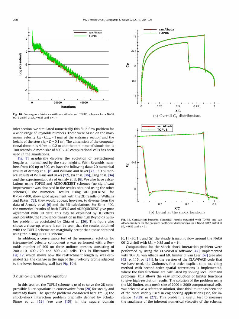
arises frequently as a model for simulating thin shear layers orsharp interfaces between inviscid fluids [52]. The solutions weremarched in time until time t = 0.8 by using a mesh size of200 � 200 computational cells and at CFL number of 0.8. Fig. 13shows density contour lines computed with TOPUS and van Albadalimiters. One can observe that TOPUS provides qualitatively thesame resolution as van Albada except at the top right region, wherethe TOPUS limiter captures the vortical structures a little better.However, when the density and pressure profiles are plotted alongthe diagonal (x = y line), as shown in Fig. 14, significant differencesbetween the TOPUS and the van Albada solutions can clearly be ob-served, indicating that TOPUS has behaved somewhat better thanthe van Albada limiter. In addition, to show that the TOPUS schemeis capable of capturing the complex interacting structures in theflow (i.e., vortex sheets), we repeat the numerical experimentshown in Fig. 13 using a mesh size of 1500 � 1500 computationalcells. The density contour lines are depicted in Fig. 15, from whichit can be seen that the TOPUS scheme provides a substantialimprovement at the contact surface, where instabilities manifestthemselves. So, it would appear that the TOPUS limiter introducesless numerical viscosity than van Albada.

We now focus on the specific AGARD test case (see [2]) of thesteady inviscid compressible flow over a NACA 0012 airfoil at free-stream Mach number M1 = 0.85 and angle-of-attack a = 1 deg. Theobjective of this test is to investigate whether the TOPUS schemecould resolve flows possessing strong shocks as well as the vanAlbada limiter, a widely used upwinding scheme for compressibleflow computations. This classical case is computed using a meshsize of 251 points over the airfoil surface, 151 points in radial direc-tion and the farfield boundary is set at 70 chords of radius. Thesolution is obtained using single-precision operations. The CFLnumber is set as a constant value of 0.7 and the maximum densityresidual for accepting convergence is chosen to be 10�7. TimeMarch to steady state uses the 5-stage, 2th-order accurate, explicitRunge–Kutta method presented in Ref. [32]. In Fig. 16, the conver-gence curves obtained with the van Albada and TOPUS schemes arepresented, showing that both schemes converge, at about the samerate, with eight orders of magnitude reduction in the residual.

The pressure coefficient distributions, Cp, on the upper andlower surfaces of the airfoil obtained with TOPUS and van Albadalimiters are plotted in Fig. 17. The overall views of the Cp distri-

butions are shown in Fig. 17a and detailed views of the upperand lower surface shock waves are shown in Fig. 17b. From thesefigures, it is seen that both TOPUS and van Albada limiters pro-vide similar results, showing that the strength of the shock is ingood agreement with the ones given in [2]. The results are alsoindicating that the shocks can be captured by the TOPUS schemewith 1–2 mesh points, whereas 3–4 points in the shock transitionare observed when the van Albada limiter is used. The data inFig. 17b also indicate that TOPUS is slightly less dissipative thanthe van Albada limiter at the shock. Away from the shock waves,both TOPUS and van Albada schemes produce almost identicalresults.

Further investigation of these results can be achieved byinspecting the entropy generated by the numerical solutions.Hence, Fig. 18 presents the entropy generated at the airfoil surfaceby the two schemes for the same flight condition. Moreover, theentropy fields are shown in Fig. 19a and b for van Albada and TO-PUS schemes, respectively. The clear conclusion from these figuresis that the entropy generated by the two schemes is quite compa-rable. In Fig. 18, one can see that TOPUS creates slightly more en-tropy at the airfoil surface than the van Albada limiter. Again, theseresults emphasize that TOPUS has essentially the same shock cap-turing characteristics as the widely used van Albada limiter forsuch inviscid transonic applications.

Finally, drag and lift coefficients (Cd and Cl) are summarized inTable 6. In this particular case, besides the comparison betweenTOPUS and van Albada schemes, we have included results for thepresent test case obtained by Amaladas and Kamath [1], Jamesonand Martinelli [33] and by Pulliam and Barton [50]. The table alsoincludes the range of values for lift and drag coefficients reportedin [2]. Such data provide for a more quantitative comparison ofthe presently proposed scheme. One can see in Table 6 that thepresent results for lift and drag coefficients are between those pro-vided by the van Albada limiter and those provided by the centeredschemes. Again, the current results are very close to those providedby the van Albada limiter, except that we obtain a slightly highervalue of lift coefficient, which is probably a consequence of the lessdissipative behavior at the shock, as previously discussed, and alsoa somewhat higher drag coefficient. We believe that the higherdrag coefficient is associated with the fact that TOPUS is generatingslightly more entropy at the airfoil surface than the van Albadalimiter, as indicated in Fig. 18. Hence, TOPUS produces more spuri-ous drag than the van Albada limiter, explaining the higher Cd val-ues. However, one should notice that, clearly, such additionalspurious drag is quite lower than what is generated by the otherschemes compared in Table 6. Furthermore, the current resultsfor both lift and drag coefficients are well within the ranges re-ported in [2].

4. Closing remarks

A high degree polynomial upwind-based finite differencescheme (TOPUS) has been introduced for the numerical solutionof convection-dominated transport problems. This new schemewas derived from the application of the TVD/CBC stability criteriacombined with the four conditions of Leonard [41]. TOPUS is pre-sented in both the normalized variables of Leonard and also as aflux limiting technique, and has been shown to possess threeimportant features: simplicity, robustness and generality of appli-cation. By setting the free parameter a equal to 2, the scheme isthen guaranteed to be oscillation-free; and, with this value of a,the performance of the scheme was evaluated by solving a varietyof test problems. These included the 1D/2D advection of scalars,the 1D Riemann problem for Euler’s/Burgers’ equation, the 2D Rie-mann problem for Euler’s equation, the 2D incompressible Navier–

X

Y

0 1

-0.5

0

0.5

1

1.5s

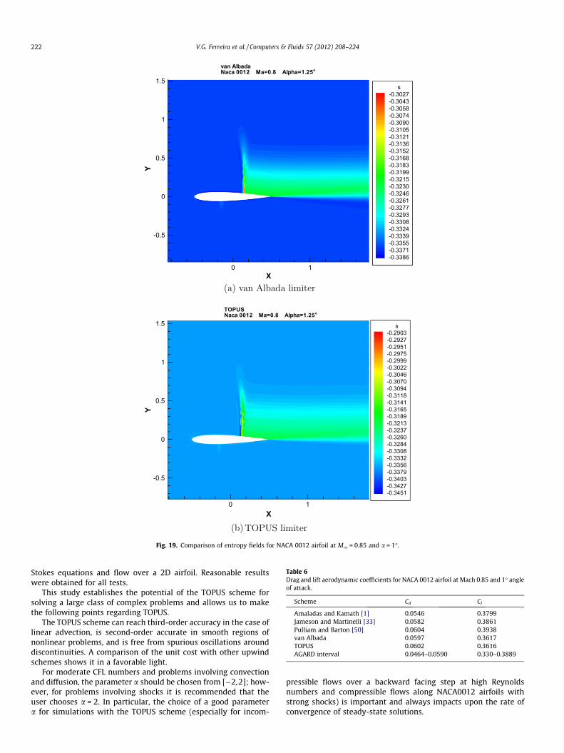
-0.3027-0.3043-0.3058-0.3074-0.3090-0.3105-0.3121-0.3136-0.3152-0.3168-0.3183-0.3199-0.3215-0.3230-0.3246-0.3261-0.3277-0.3293-0.3308-0.3324-0.3339-0.3355-0.3371-0.3386

van AlbadaNaca 0012 Ma=0.8 Alpha=1.25o

X

Y

0 1

-0.5

0

0.5

1

1.5 s-0.2903-0.2927-0.2951-0.2975-0.2999-0.3022-0.3046-0.3070-0.3094-0.3118-0.3141-0.3165-0.3189-0.3213-0.3237-0.3260-0.3284-0.3308-0.3332-0.3356-0.3379-0.3403-0.3427-0.3451

TOPUSNaca 0012 Ma=0.8 Alpha=1.25o

Fig. 19. Comparison of entropy fields for NACA 0012 airfoil at M1 = 0.85 and a = 1�.

Table 6Drag and lift aerodynamic coefficients for NACA 0012 airfoil at Mach 0.85 and 1� angleof attack.

Scheme Cd Cl

Amaladas and Kamath [1] 0.0546 0.3799Jameson and Martinelli [33] 0.0582 0.3861Pulliam and Barton [50] 0.0604 0.3938van Albada 0.0597 0.3617TOPUS 0.0602 0.3616AGARD interval 0.0464–0.0590 0.330–0.3889

222 V.G. Ferreira et al. / Computers & Fluids 57 (2012) 208–224

Stokes equations and flow over a 2D airfoil. Reasonable resultswere obtained for all tests.

This study establishes the potential of the TOPUS scheme forsolving a large class of complex problems and allows us to makethe following points regarding TOPUS.

The TOPUS scheme can reach third-order accuracy in the case oflinear advection, is second-order accurate in smooth regions ofnonlinear problems, and is free from spurious oscillations arounddiscontinuities. A comparison of the unit cost with other upwindschemes shows it in a favorable light.

For moderate CFL numbers and problems involving convectionand diffusion, the parameter a should be chosen from [�2,2]; how-ever, for problems involving shocks it is recommended that theuser chooses a = 2. In particular, the choice of a good parametera for simulations with the TOPUS scheme (especially for incom-

pressible flows over a backward facing step at high Reynoldsnumbers and compressible flows along NACA0012 airfoils withstrong shocks) is important and always impacts upon the rate ofconvergence of steady-state solutions.

V.G. Ferreira et al. / Computers & Fluids 57 (2012) 208–224 223

The 1D numerical results in this paper show that TOPUS is a ro-bust strategy for capturing shocks while maintaining a non-oscilla-tory profile, and when compared with reference solutions and thebest existing schemes, TOPUS does as well and occasionally better.

However, although TOPUS competes well with existingschemes, such as SMARTER, 3rd WENO, MUSCL and ADBQUICKEST,it is certainly not always better. Its main advantage lies in the sys-tematic nature of the scheme, its low cost and its fast implementa-tion for prototyping and fluid model verification/validation.

In particular, TOPUS provides practically the same resolution asADBQUICKEST without the need to tune the Courant parameter ateach time step, and requires less computational time.

Overall, the TOPUS scheme is an alternative to the family of up-wind schemes for simulating shock wave propagation and otherphenomena where the nonlinear advection term requires specialattention. We have numerically shown that the method can solvenonstationary as well as stationary problems in two space vari-ables. In the transonic inviscid flow over NACA0012 airfoil compu-tation, for example, TOPUS provided results compatible both withthat given by van Albada and existing experimental data. However,as a perspective for improvement of steady compressible flow cal-culations, an extra effort will have to be undertaken in the future inorder to couple the TOPUS scheme with an efficient implicit solver.For incompressible flows, TOPUS has proved to be an effective toolfor resolving the delicate features and structures of a laminar flowover a backward facing step.

Acknowledgments

Financial support from the FAPESP under Grants 05/51458-0,06/05910-1, 08/02673-4, 09/16954-8, 04/16064-9, and 09/15892-9 as well as CNPq under Grants 304201/2005-7, 312064/2006-3,477858/2009-0 and 305447/2010-6 are gratefully appreciated.This work was also carried out in the framework of the InstitutoNacional de Ciência e Tecnologia em Medicina Assistida porComputação Científica (CNPq, Brazil).

References

[1] Amaladas JR, Kamath H. Accuracy assessment of upwind algorithms forsteady-state computations. Comput Fluids 1998;93:941–62.

[2] AGARD Subcommittee C. Test cases for inviscid flow field methods, AGARDadvisory report 211; 1985. p. 6–27.

[3] Ahmed R. Numerical schemes applied to the burgers and Buckley–Leverettequations. MSc dissertation, University of Reading; 2004.

[4] Alves MA, Pinho FT, Oliveira. Effect of a high-resolution differencing scheme onfinite-volume predictions of viscoelastic flows. J Non-Newton Fluid Mech2000;93:287–314.

[5] Alves MA, Oliveira PJ, Pinho FT. A convergent and universally boundedinterpolation scheme for the treatment of advection. Int J Numer MethodsFluids 2003;41:47–75.

[6] Armaly BF, Durst F, Pereira JCF, Schonung B. Experimental and theoreticalinvestigation of backward facing step flow. J Fluid Mech 1983;127:473–96.

[7] Arora M, Roe PL. A well-behaved TVD limiter for high-resolution calculations ofunsteady flow. J Comput Phys 1997;132:3–11.

[8] Barth TJ, Jespersen DC. The design and application of upwind schemes onunstructured meshes. AIAA paper 89-0366. In: 27th AIAA aerospace sciencesmeeting, Reno, NV; 1989.

[9] Balsara DS, Shu CW. Monotonicity preserving weighted essentially non-oscillatory schemes with increasingly high order of accuracy. J Comput Phys2000;160:405–52.

[10] Berthon C. Stability of the MUSCL schemes for the Euler equations. CommunMath Sci 2005;3:133–57.

[11] Bigarella EDV. Advanced turbulence modelling for complex aerospaceapplications. PhD thesis, Sao Jose dos Campos; 2007.

[12] Bigarella EDV, Azevedo JLF. Advanced eddy-viscosity and Reynolds-stressturbulence model simulations of aerospace applications. AIAA paper no. 2006-2826. In: 24th AIAA applied aerodynamics conference, San Francisco, CA, USA,vol. 1; 2006. p. 1–39.

[13] Brandt A, Yavneh I. Inadequacy of first-order upwind difference schemes forsome recirculating flows. J Comput Phys 1991;93:128–43.

[14] Burgers JM. A mathematical model illustrating the theory of turbulence. AdvAppl Mech 1948;1:171–99.

[15] Cada M, Torrilhon M. Compact third-order limiter functions for finite volumemethods. J Comput Phys 2009;228:4118–45.

[16] Castelo A, Tomé MF, Cesar CNL, McKee S, Cuminato JA. Freeflow: an integratedsimulation system for three-dimensional free surface flows. J Comput VisualSci 2000;2:1–12.

[17] Chakravarthy SR, Osher S. High resolution applications of the Osher upwindscheme for the Euler equations, AIAA paper 83-1943. In: 6th Computationalfluid dynamics conference; 1983. p. 363–73.

[18] Chassignet EP, Hurlburt HE, Smedstad OM, Halliwell GR, Hogan PJ, WallcraftAJ, et al. The HYCOM (HYbrid Coordinate Ocean Model) data assimilativesystem. J Marine Syst 2007;65:60–83.

[19] Choi SK, Nam HY, Cho M. A comparison of higher-order bounded convectionschemes. Comput Methods Appl Mech Eng 1995;121:281–301.

[20] Chorin AJ. Numerical solution of the Navier–Stokes equations. Math Comput1968;22:745–62.

[21] Courant R, Isaacson E, Rees M. On the solution of nonlinear hyperbolicdifferential equations by finite differences. Commun Pure Appl Math1952;5:243–55.

[22] Corre C, Lerat A. High-order residual-based compact schemes for advection–diffusion problems. Comput Fluids 2008;37:505–19.

[23] Ferreira VG, Kurokawa FA, Queiroz RAB, Kaibara MK, Oishi CM, Cuminato JA,et al. Assessment of a high-order finite difference upwind scheme for thesimulation of convection–diffusion problems. Int J Numer Methods Fluids2009;60:1–26.

[24] Gaskell PH, Lau AKC. Curvature-compensated convective transport: SMART, anew boundedness-preserving transport algorithm. Int J Numer Methods Fluids1988;8:617–41.

[25] Gauzha VG, Vorozhtsov EV. Numerical solutions for partial differentialequations. New York: CRC Press; 1996.

[26] Ghia KN, Osswald GA, Ghia U. Analysis of incompressible massively separatedviscous flows using unsteady Navier–Stokes equations. Int J Numer MethodsFluids 1989;9:1025–50.

[27] Godoy WF, Desjardin PE. On the use of flux limiters in the discrete ordinatesmethod for 3D radiation calculations in absorbing and scattering media. JComput Phys 2010;229:3189–213.

[28] Goodman JB, LeVeque RJ. A geometric approach to high resolution TVDschemes. SIAM J Numer Anal 1988;25:268–84.

[29] Harten A. High resolution schemes for hyperbolic conservation laws. J ComputPhys 1983;49:357–93.

[30] Harlow FH, Welch JE. Numerical calculation of time-dependent viscousincompressible flow of fluid with free surface. Phys Fluids 1965;8:2182–9.

[31] Hubbard ME, Garcia-Navarro P. Flux difference splitting and the balancing ofsource terms and flux gradients. J Comput Phys 2000;165:89–125.

[32] Jameson A, Mavriplis D. Finite volume solution of the two-dimensional Eulerequations on a regular triangular mesh. AIAA J 1986;24:611–8.

[33] Jameson A, Martinelli L. Mesh refinement and modeling errors in flowsimulation. AIAA J 1998;36:676–86.

[34] Jiang G-S, Shu C-W. Efficient implementation of weighted ENO scheme. JComput Phys 1996;126:202–28.

[35] Koren B. Upwind discretization of the steady Navier–Stokes equations. Int JNumer Methods Fluids 1990;11:99–117.

[36] Ku HC, Hirsch RS, Taylor TD, Rosenberg AP. A pseudospectral matrix elementmethod for solution of the dimensional incompressible flows and its parallelimplementations. J Comput Phys 1989;83:260–91.

[37] Kuan KB, Lin CA. Adaptive QUICK-based scheme to approximate convectivetransport. AIAA J 2000;38:2233–7.

[38] Lee L. A class of high-resolution algorithms for incompressible flows. ComputFluids 2010;39:1022–32.

[39] Leonard BP. A stable and accurate convective modelling procedure based onquadratic upstream interpolation. Comput Methods Appl Mech Eng1990;19:59–98.

[40] Leonard BP. Universal limiter for transient interpolation modeling of theadvective transport equations: the ULTIMATE conservative difference scheme,NASA Technical Memorandum 100916, ICOMP-88-11; 1988.

[41] Leonard BP. Simple high-accuracy resolution program for convective modelingof discontinuities. Int J Numer Methods Fluids 1988;8:1291–318.

[42] LeVeque RJ. Finite volume methods for hyperbolic problems. NewYork: Cambridge University Press; 2002.

[43] Lin H, Chieng CC. Characteristic-based flux limiter of an essentially third-orderflux-splitting method for hyperbolic conservation laws. Int J Numer MethodsFluids 1991;13:287–307.

[44] Lin C-H, Lin CA. Simple high-order bounded convection scheme to modeldiscontinuities. AIAA J 1997;35:563–5.

[45] McKee S, Tomé MF, Ferreira VG, Cuminato JA, Castelo A, Sousa FS, et al. TheMAC method. Comput Fluids 2008;37:907–30.

[46] Naterer GF. Constructing an entropy-stable upwind scheme for compressiblefluid flow. AIAA J 1999;37:303–12.

[47] Osher S. Convergence of generalized MUSCL schemes. SIAM J Numer Anal1985;22:947–61.

[48] Patankar SV. Numerical heat transfer and fluid flows. New York: HemispherePublishing Corporation; 1980.

[49] Piperno S, Depeyre S. Criteria for the design of limiters yielding efficient highresolution TVD schemes. Int J Numer Methods Fluids 1998;27:183–97.

[50] Pulliam TH, Barton JT. Euler computations of AGARD working 07 airfoil testcases. AIAA paper, 85-0018; 1985.

224 V.G. Ferreira et al. / Computers & Fluids 57 (2012) 208–224

[51] Roe P, Pike J. Efficient construction and utilization of approximate Riemannsolutions. Comput Methods Appl Sci Eng 1984;6:499–518.

[52] Samtaney R, Pullin DI. On initial-value and self-similar solutions of thecompressible Euler equations. Phys Fluids 1996;8:2650–5.

[53] Schulz-Rinne CW, Collins JP, Glaz HM. Numerical solution of the Riemannproblem for two-dimensional gas dynamics. SIAM J Sci Comput 1993;14:1394–414.

[54] Smith RM, Hutton AG. The numerical treatment of advection: a performancecomparison of currents methods. Numer Heat Transfer 1982;5:439–61.

[55] Shin JK, Choi YD. Study on the improvement of the convective differencingscheme for the high-accuracy and stable resolution of the numerical solution.Trans KSME 1992;16:345–60.

[56] Shu C-W, Osher S. Efficient implementation of essentially non-oscillatoryshock capturing schemes. J Comput Phys 1989;83:32–78.

[57] Song B, Liu GR, Lam KY, Amano RS. On a higher-order bounded discretizationscheme. Int J Numer Methods Fluids 2000;32:881–97.

[58] Spalding DB. A novel finite difference formulation for differential expressionsinvolving both first and second derivatives. Int J Numer Methods Eng1972;4:551–9.

[59] Strikwerda JG. Upwind differencing, false scaling, and nonphysical solutions tothe driven cavity problem. J Comput Phys 1982;47:303–7.

[60] Sweby PK. High resolution schemes using flux limiters for hyperbolicconservation laws. SIAM J NumerAnal 1984;21:995–1011.

[61] Tang H, Warnecke G. A Runge–Kutta discontinuous Galerkin method for theEuler equations. Comput Fluids 2005;34:375–98.

[62] Toro EF. Riemann solver and numerical methods for fluid dynamics. 2nded. Berlin (Heidelberg): Springer-Verlag; 1999.

[63] Tremback CJ, Powell J, Cotton WR, Pielke RA. The forward in-time upstreamadvection scheme: extension to higher orders. Mon Weather Rev 1987;115:540–55.

[64] van Albada GD, van Leer B, Roberts WW. A comparative study ofcomputational methods in cosmic gas dynamics. Astron Astrophys1982;108:76–84.

[65] Varonos A, Bergeles G. Development and assessment of a variable-order non-oscillatory scheme for convection term discretization. Int J Numer MethodsFluids 1998;26:1–16.

[66] van Leer B. Towards the ultimate conservative difference scheme II.Monotonicity and conservation combined in a second-order scheme. JComput Phys 1974;14:361–70.

[67] van Leer B. Towards the ultimate conservative difference scheme IV. A newapproach to numerical convection. J Comput Phys 1977;23:276–99.

[68] van Leer B. Towards the ultimate conservative difference scheme V. A second-order sequel to Godunov’s method. J Comput Phys 1979;32:101–36.

[69] van Leer B. Upwind and high-resolution methods for compressible flow: fromdonor cell to residual-distribution schemes. Commun Comput Phys2006;1:192–206.

[70] Warming RF, Beam RM. Upwind second-order difference schemes andapplications in aerodynamic flows. AIAA J 1976;14:1241–9.

[71] Waterson NP, Deconinck H. Design principles for bounded higher-orderconvection schemes – a unified approach. J Comput Phys 2007;224:182–207.

[72] Williams PT, Baker AJ. Numerical simulations of laminar flow over a 3Dbackward-facing step. Int J Numer Methods Fluids 1997;24:1159–83.

[73] Xue S-C, Phan-Thien N, Tanner RI. Upwinding with deferred correction(UPDC): an effective implementation of higher-order convection schemes forimplicit finite volume methods. J Non-Newton Fluid Mech 2002;108:1–24.

[74] Yamaleev NK, Carpenter MH. Third-order energy stable WENO scheme. JComput Phys 2009;228:3025–47.

[75] Zhang J, Jackson TL. A high-order incompressible flow solver with WENO. JComput Phys 2009;228:2426–42.

[76] Zijlema M. On the construction of a third-order accurate monotone convectionscheme with application to turbulent flows in general domains. Int J NumerMethods Fluids 1996;22:619–41.

[77] Zhou G, Davidson L, Olsson E. Transonic inviscid/turbulent airfoil flowsimulations using a pressure based method with high order schemes. LectNotes Phys 1995;453:372–7.

[78] Zhou T, Li Y, Shu C-W. Numerical comparison of WENO finite volume andRunge–Kutta discontinuos Galerkin methods. J Sci Comput 2001;16:145–71.

[79] Zhu J. On the higher-order bounded discretization schemes for finite volumecomputations of incompressible flows. Comput Methods Appl Mech Eng1992;98:345–60.