Computers and Fluids -...
19
Computers and Fluids 168 (2018) 285–303 Contents lists available at ScienceDirect Computers and Fluids journal homepage: www.elsevier.com/locate/compfluid An aerodynamic design optimization framework using a discrete adjoint approach with OpenFOAM Ping He a,∗ , Charles A. Mader a , Joaquim R.R.A. Martins a , Kevin J. Maki b a Department of Aerospace Engineering, University of Michigan, Ann Arbor, Michigan 48109, USA b Department of Naval Architecture and Marine Engineering, University of Michigan, Ann Arbor, Michigan 48109, USA a r t i c l e i n f o Article history: Received 8 November 2017 Revised 9 March 2018 Accepted 6 April 2018 Available online 7 April 2018 Keywords: OpenFOAM Discrete adjoint optimization Parallel graph coloring Ahmed body UAV Car a b s t r a c t Advances in computing power have enabled computational fluid dynamics (CFD) to become a crucial tool in aerodynamic design. To facilitate CFD-based design, the combination of gradient-based optimization and the adjoint method for computing derivatives can be used to optimize designs with respect to a large number of design variables. Open field operation and manipulation (OpenFOAM) is an open source CFD package that is becoming increasingly popular, but it currently lacks an efficient infrastructure for constrained design optimization. To address this problem, we develop an optimization framework that consists of an efficient discrete adjoint implementation for computing derivatives and a Python inter- face to multiple numerical optimization packages. Our adjoint optimization framework has the following salient features: (1) The adjoint computation is efficient, with a computational cost that is similar to that of the primal flow solver and scales up to 10 million cells and 1024 CPU cores. (2) The adjoint deriva- tives are fully consistent with those generated by the flow solver with an average error of less than 0.1%. (3) The adjoint framework can handle optimization problems with more than 100 design variables and various geometric and physical constraints such as volume, thickness, curvature, and lift constraints. (4) The framework includes additional modules that are essential for successful design optimization: a geometry-parametrization module, a mesh-deformation algorithm, and an interface to numerical opti- mizations. To demonstrate our design-optimization framework, we optimize the ramp shape of a simple bluff geometry and analyze the flow in detail. We achieve 9.4% drag reduction, which is validated by wind tunnel experiments. Furthermore, we apply the framework to solve two more complex aerodynamic- shape-optimization applications: an unmanned aerial vehicle, and a car. For these two cases, the drag is reduced by 5.6% and 12.1%, respectively, which demonstrates that the proposed optimization framework functions as desired. Given these validated improvements, the developed techniques have the potential to be a useful tool in a wide range of engineering design applications, such as aircraft, cars, ships, and turbomachinery. © 2018 Elsevier Ltd. All rights reserved. 1. Introduction Open field operation and manipulation (OpenFOAM) is an open source software package for computational fluid dynamics (CFD) [1,2] that contains more than 80 solvers capable of simulating var- ious types of flow processes, including aerodynamics, hydrodynam- ics, heat transfer, and multiphase flow [3]. OpenFOAM is being ac- tively developed and verified by its users and developers [4–7], and its popularity has been rapidly growing over the past decade. OpenFOAM has become a powerful tool for aerodynamic design of engineering systems such as aircraft, cars, and turbomachinery ∗ Corresponding author. E-mail address: [email protected] (P. He). [8–14]. One of the major tasks in the process of aerodynamic de- sign is to improve system performance (e.g., reduce drag, maximize power, and improve efficiency). Traditionally, it involves manual loops of design modification and performance evaluation, which is not efficient. To improve the efficiency of this process, the combi- nation of gradient-based optimization and the adjoint method for computing derivatives can be used to automatically optimize the design. The true benefit of using the adjoint method to compute derivatives is that its computational cost is almost independent of the number of design variables, which enables complex industrial design optimization. Given this background, the development of an adjoint optimization framework may facilitate the existing process of OpenFOAM-based aerodynamic-shape design. The adjoint method was first introduced to fluid mechanics by Pironneau [15] in 1970s. The approach was then extended by https://doi.org/10.1016/j.compfluid.2018.04.012 0045-7930/© 2018 Elsevier Ltd. All rights reserved.
Transcript of Computers and Fluids -...

Computers and Fluids 168 (2018) 285–303
Contents lists available at ScienceDirect
Computers and Fluids
journal homepage: www.elsevier.com/locate/compfluid
An aerodynamic design optimization framework using a discrete
adjoint approach with OpenFOAM
Ping He
a , ∗, Charles A. Mader a , Joaquim R.R.A. Martins a , Kevin J. Maki b
a Department of Aerospace Engineering, University of Michigan, Ann Arbor, Michigan 48109, USA b Department of Naval Architecture and Marine Engineering, University of Michigan, Ann Arbor, Michigan 48109, USA
a r t i c l e i n f o
Article history:
Received 8 November 2017
Revised 9 March 2018
Accepted 6 April 2018
Available online 7 April 2018
Keywords:
OpenFOAM
Discrete adjoint optimization
Parallel graph coloring
Ahmed body
UAV
Car
a b s t r a c t
Advances in computing power have enabled computational fluid dynamics (CFD) to become a crucial tool
in aerodynamic design. To facilitate CFD-based design, the combination of gradient-based optimization
and the adjoint method for computing derivatives can be used to optimize designs with respect to a
large number of design variables. Open field operation and manipulation (OpenFOAM) is an open source
CFD package that is becoming increasingly popular, but it currently lacks an efficient infrastructure for
constrained design optimization. To address this problem, we develop an optimization framework that
consists of an efficient discrete adjoint implementation for computing derivatives and a Python inter-
face to multiple numerical optimization packages. Our adjoint optimization framework has the following
salient features: (1) The adjoint computation is efficient, with a computational cost that is similar to that
of the primal flow solver and scales up to 10 million cells and 1024 CPU cores. (2) The adjoint deriva-
tives are fully consistent with those generated by the flow solver with an average error of less than
0.1%. (3) The adjoint framework can handle optimization problems with more than 100 design variables
and various geometric and physical constraints such as volume, thickness, curvature, and lift constraints.
(4) The framework includes additional modules that are essential for successful design optimization: a
geometry-parametrization module, a mesh-deformation algorithm, and an interface to numerical opti-
mizations. To demonstrate our design-optimization framework, we optimize the ramp shape of a simple
bluff geometry and analyze the flow in detail. We achieve 9.4% drag reduction, which is validated by wind
tunnel experiments. Furthermore, we apply the framework to solve two more complex aerodynamic-
shape-optimization applications: an unmanned aerial vehicle, and a car. For these two cases, the drag is
reduced by 5.6% and 12.1%, respectively, which demonstrates that the proposed optimization framework
functions as desired. Given these validated improvements, the developed techniques have the potential
to be a useful tool in a wide range of engineering design applications, such as aircraft, cars, ships, and
turbomachinery.
© 2018 Elsevier Ltd. All rights reserved.
1
s
[
i
i
t
a
O
o
[
s
p
l
n
n
c
d
d
t
d
h
0
. Introduction
Open field operation and manipulation (OpenFOAM) is an open
ource software package for computational fluid dynamics (CFD)
1,2] that contains more than 80 solvers capable of simulating var-
ous types of flow processes, including aerodynamics, hydrodynam-
cs, heat transfer, and multiphase flow [3] . OpenFOAM is being ac-
ively developed and verified by its users and developers [4–7] ,
nd its popularity has been rapidly growing over the past decade.
penFOAM has become a powerful tool for aerodynamic design
f engineering systems such as aircraft, cars, and turbomachinery
∗ Corresponding author.
E-mail address: [email protected] (P. He).
a
o
b
ttps://doi.org/10.1016/j.compfluid.2018.04.012
045-7930/© 2018 Elsevier Ltd. All rights reserved.
8–14] . One of the major tasks in the process of aerodynamic de-
ign is to improve system performance (e.g., reduce drag, maximize
ower, and improve efficiency). Traditionally, it involves manual
oops of design modification and performance evaluation, which is
ot efficient. To improve the efficiency of this process, the combi-
ation of gradient-based optimization and the adjoint method for
omputing derivatives can be used to automatically optimize the
esign. The true benefit of using the adjoint method to compute
erivatives is that its computational cost is almost independent of
he number of design variables, which enables complex industrial
esign optimization. Given this background, the development of an
djoint optimization framework may facilitate the existing process
f OpenFOAM-based aerodynamic-shape design.
The adjoint method was first introduced to fluid mechanics
y Pironneau [15] in 1970s. The approach was then extended by

286 P. He et al. / Computers and Fluids 168 (2018) 285–303
S
w
c
p
a
g
m
i
c
a
d
t
t
(
a
d
g
a
w
2
j
f
a
a
s
f
P
u
t
[
a
m
j
f
2
f
d
m
t
d
g
r
P
O
s
i
s
a
fl
d
o
p
p
w
Jameson [16] to the optimization of two-dimensional aerodynamic-
shape design in the late 1980s. Since then, the adjoint method has
been implemented for three-dimensional turbulent flows, and its
application has also been generalized to multipoint and multidis-
ciplinary design optimization [17–26] . While the adjoint method
is recognized as an efficient method for computing derivatives of
a solver based on partial differential equations (PDEs), success-
ful optimization requires a framework that includes other compo-
nents that go beyond the flow solution and derivative computation.
We also require modules for geometry manipulation, mesh defor-
mation, and optimization algorithms. The speed and accuracy of
such modules, especially as they pertain to derivative computation,
strongly impact the overall optimization. We have developed a full
suite of modules to facilitate aerodynamic optimization, some of
which have been published previously. The geometry-manipulation
module was developed by Kenway et al. [27] and has been used in
various aerodynamic and aerostructural design-optimization stud-
ies [26,28–31] . Perez et al. [32] developed an open source Python
interface to various numerical optimization packages that we reuse
here. 1 In the present work, we focus on the implementation of the
adjoint solver in OpenFOAM, the development of which allows the
OpenFOAM solver to be efficiently integrated into our existing op-
timization framework.
Two different methods exist for formulating the adjoint of a
flow solver: continuous and discrete [33] . The continuous approach
derives the adjoint formulation from the Navier–Stokes (NS) equa-
tions and then discretizes to obtain the numerical solution. In con-
trast, the discrete approach starts from the discretized NS equa-
tions and differentiates the discretized equations to get the adjoint
terms. Although these two approaches handle adjoint formulation
in different ways, they both converge to the same answer for a suf-
ficiently refined mesh [34] .
The adjoint method was first implemented in OpenFOAM by
Othmer [35] , who used the continuous approach to derive the ad-
joint formulation for the incompressible flow solver simpleFoam.
This continuous adjoint implementation was then integrated as
a built-in OpenFOAM solver for computing derivatives. A num-
ber of recent studies have reported shape optimization based on
derivatives computed from the continuous adjoint [36–40] . Oth-
mer’s continuous adjoint framework uses a free-form deformation
(FFD) geometry-morphing technique that can handle complex ge-
ometries such as full-scale cars. Moreover, the computational cost
for the adjoint is similar to that for the primal flow solver, allowing
one to tackle cases with more than 10 million cells [38,39] . How-
ever, they used a basic steepest descent optimization algorithm to
update the shape, so their optimization problems did not include
design constraints.
More recently, Towara and Naumann [41] reported a discrete
adjoint implementation for OpenFOAM. They used reverse mode
automatic differentiation (AD) to compute derivatives so that the
adjoint derivatives are fully consistent with the flow solution, re-
gardless of the mesh refinement. However, they used AD to dif-
ferentiate the entire OpenFOAM code, requiring all flow variables
to be stored to conduct the reverse AD computation. To reduce
the memory required to store the flow variables, the checkpoint-
ing technique was used to trade speed for memory. As a result,
the overall computational cost to compute derivatives is high—the
adjoint-flow runtime ratio ranges from 5 to 15 [42–44] . Given the
cost of this adjoint computation, it would be hard to use this im-
plementation for practical shape optimization.
Instead of applying AD to the entire code, we implement a
discrete adjoint approach where the partial derivatives in the
adjoint equations are computed by using finite differences (see
1 https://www.github.com/mdolab/pyoptsparse .
i
a
m
ection 2.5 ). The objective here is to develop an adjoint solver
ithin the limitations of the OpenFOAM framework that is suffi-
iently efficient for practical shape optimization. We evaluate the
erformance of our adjoint implementation in terms of speed, scal-
bility, and accuracy, optimize the aerodynamic shape of a bluff
eometry representative of a ground vehicle, and validate the opti-
ized result by comparing it with the result of wind tunnel exper-
ments. Furthermore, we demonstrate the constrained optimization
apability for two more complex shape-optimization applications:
n unmanned aerial vehicle (UAV), and a car. We opt to use the
iscrete adjoint approach because the adjoint derivative is consis-
ent with the flow solution, as mentioned above. Moreover, we find
he discrete adjoint implementation easier to maintain and extend
for example, when adding new objective or constraint functions
nd boundary conditions).
The rest of the paper is organized as follows: Section 2 intro-
uces the optimization framework along with the theoretical back-
round for each of its modules. Section 3 evaluates its performance
nd presents the aerodynamic shape optimization results. Finally,
e summarize and give conclusions in Section 4 .
. Methodology
The design-optimization framework implements a discrete ad-
oint for computing the total derivative d f/ d x , where f is the
unction of interest (which for optimization will be the objective
nd constraint functions, e.g., drag, lift, and pitching moment),
nd x represents the design variables that control the geometric
hape via FFD control point movements. The design-optimization
ramework consists of multiple components written in C ++ and
ython and depends on the following external libraries and mod-
les: OpenFOAM, portable, extensible toolkit for scientific compu-
ation (PETSc) [45,46] , pyGeo [27] , pyWarp [27] , and pyOptSparse
32] . The framework also requires an external optimization pack-
ge, which can be any package supported by the pyOptSparse opti-
ization interface. In this section, we elaborate on the overall ad-
oint optimization framework, the theoretical background for the
ramework modules, and the code structure and implementation.
.1. Discrete adjoint optimization framework
Fig. 1 shows the modules and data flow for the optimization
ramework. We use the extended design structure matrix standard
eveloped by Lambe and Martins [47] . The diagonal entries are the
odules in the optimization process, whereas the off-diagonal en-
ries are the data. Each module takes data input from the vertical
irection and outputs data in the horizontal direction. The thick
ray lines and thin black lines denote the data and process flow,
espectively. The numbers in the entries are their execution order.
The framework consists of two major layers: OpenFOAM and
ython, and they interact through input and output files. The
penFOAM layer consists of a flow solver (simpleFoam), an adjoint
olver (discreteAdjointSolver), and a graph-coloring solver (color-
ngSolver). The flow solver is based on the standard OpenFOAM
olver simpleFoam for steady incompressible turbulent flow. The
djoint solver computes the total derivative d f/ d x based on the
ow solution generated by simpleFoam. The mesh deformation
erivative matrix ( d x v / d x , where x v contains the volume-mesh co-
rdinates) is needed when computing the total derivative and is
rovided by the Python layer. To accelerate computation of the
artial derivatives, we developed a parallel graph-coloring solver,
hose algorithm is discussed in Section 2.6 .
The Python layer is a high-level interface that takes the user
nput and the total derivatives computed by the OpenFOAM layer
nd calls multiple external modules to perform constrained opti-
ization. To be more specific, these external modules include “py-

P. He et al. / Computers and Fluids 168 (2018) 285–303 287
Fig. 1. Extended design-structure matrix [47] for discrete adjoint framework for constrained-shape-optimization problems. x : design variables; x (0) : baseline design variables;
x ( ∗) : optimized design variables; x S : coordinates of design surface; x V : coordinates of volume mesh; w : state variables; c : geometric constraints; f : objective and constraint
functions.
G
o
f
t
t
v
t
s
d
f
2
g
[
g
i
s
s
o
c
t
u
p
v
i
c
m
d
g
a
t
c
2
c
s
t
m
i
fi
b
h
t
r
t
p
t
m
q
m
e
n
m
2
t
t
t∫
∫w
l
t
a
T
m
a
e
t
l
eo” for the surface-geometry parameterization and computation
f geometric constraints c and their derivatives d c /d x , “pyWarp”
or the volume-mesh deformation, and “pyOptSparse” for the op-
imization setup. In this paper, we use the sparse nonlinear op-
imizer (SNOPT) package [48] , but the pyOptSparse interface pro-
ides access to various other optimization algorithms. In addition,
he PETSc library is used to efficiently manipulate and store large
parse matrices and vectors and to solve the linear equations. The
etailed background for each of these modules is introduced in the
ollowing sections.
.2. Surface geometry parameterization—pyGeo
To optimize the shape, one must manipulate the surface of a
iven geometry. We use a FFD implementation by Kenway et al.
27] to parameterize geometries. The FFD approach embeds the
eometry into a volume that can then be manipulated by mov-
ng points at the surface of that volume (the FFD points). Fig. 2 (a)
hows an example of using the FFD approach to parameterize the
urface of a bluff geometry called the Ahmed body [49] . Once an
bject is embedded into a FFD volume, a Newton search is exe-
uted to determine the mapping between the FFD points (parame-
er space) and the surface geometry (physical space). The FFD vol-
me is a trivariate B -spline volume such that the gradient of any
oint inside the volume can be easily computed. Note that the FFD
olume parameterizes the geometry changes rather than chang-
ng the geometry itself, allowing us to choose a more efficient and
ompact set of design variables.
The geometry parameterization is implemented in the pyGeo
odule and allows us to control the local shape of the geometry
uring optimization. Moreover, by moving sets of FFD points to-
ether, one can produce rigid motion for surface deformation. This
llows us to control the global dimension of a geometry, such as
he ramp angle of the Ahmed body, or the twist, sweep, span, and
hord of an aircraft wing.
.3. Volume mesh deformation—pyWarp
Once the surface geometry is changed in the optimization pro-
ess, the corresponding changes need to be applied to the CFD
urface mesh. To avoid having negative-volume cells and to main-
ain mesh quality, we also need to smoothly deform the volume
esh; a process also known as mesh warping or mesh morph-
ng. The mesh-deformation algorithm used in this work is an ef-
cient analytic inverse-distance method similar to that described
y Luke et al. [50] . The advantage of this approach is that it is
ighly flexible and can be applied to both structured and unstruc-
ured meshes. In addition, compared with the method based on
adial basis functions [51] , this approach better preserves mesh or-
hogonality in the boundary layer. Figs. 2 (b) and (c) show exam-
les of the baseline and deformed volume mesh in the symme-
ry plane for the Ahmed body. The surface-parameterization and
esh-deformation operations are fully parallel and typically re-
uire less than 0.1% of the CFD simulation time. Such a speedy
esh deformation is crucial when optimizing, because this op-
ration is called multiple times for each optimization iteration;
amely, when the surface geometry is updated and when the
esh-deformation derivative matrix d x v / d x is computed.
.4. SIMPLE-algorithm-based solver for steady incompressible
urbulent flow—simpleFoam
The standard OpenFOAM solver simpleFoam is used to simulate
he steady incompressible turbulent flow by solving the NS equa-
ions:
S
U · d S = 0 , (1)
S
U U · d S +
∫ V
∇p d V −∫
S
(ν + νt )(∇ U + ∇ U
T ) · d S = 0 , (2)
here U = [ u , v , w ] is the velocity vector; u , v , and w are the ve-
ocity components in the x , y , and z directions, respectively; S is
he face-area vector; V is the volume; ν and νt are the molecular
nd turbulent eddy viscosity, respectively; and p is the pressure.
he finite volume method is used to discretize the continuity and
omentum equations on collocated meshes. These two equations
re coupled by using the semi-implicit method for pressure-linked
quations (SIMPLE) algorithm [52] along with the Rhie–Chow in-
erpolation [53] . The detailed implementation is given below, fol-
owing Jasak [54] .

288 P. He et al. / Computers and Fluids 168 (2018) 285–303
Fig. 2. (a) Surface-geometry parameterization for Ahmed body [49] obtained by using FFD approach. The black and red squares are the FFD points. Only the black FFD points
are selected as the design variables for manipulating the ramp shape whereas the red FFD points remain unchanged during the optimization. (b) Baseline and (c) deformed
volume mesh at symmetry plane for Ahmed body. The surface parameterization and mesh-deformation operations are fully parallel and typically require less than 0.1% of
the CFD simulation time.
I
c
f
l
U
T
R
b
s
t
∇
S
fl
φ
N
u
u
t
The SIMPLE algorithm starts by discretizing the momentum
equation and solving an intermediate velocity field by using the
pressure field obtained from the previous iteration or an initial
guess ( p 0 ). The momentum equation is then semi-discretized as
a P U P = −∑
N
a N U N − ∇p 0 = H ( U ) − ∇p 0 , (3)
where a is the coefficient resulting from the finite-volume dis-
cretization, subscripts P and N denote the control volume cell and
all of its neighboring cells, respectively, and H ( U ) = − ∑
N a N U N
represents the influence of the velocity from all the neighboring
cells. Note that, to linearize the convective term, a new variable
φ0 (the cell-face flux) is introduced into the discretization to give∫ S
U U · d S =
∑
f
U f U f · S f =
∑
f
φ0 U f , (4)
where the subscript f denotes the cell face. The cell-face flux φ0
can be obtained from the previous iteration or from an initial
guess. The above linearization process complicates the discrete ad-
joint implementation; we elaborate on this issue and its solution
in Section 2.5 . Solving Eq. (3) , we obtain an intermediate velocity
field that does not yet satisfy the continuity equation.
Next, the continuity equation is coupled with the momentum
equation to construct a pressure Poisson equation, and a new
pressure field is computed. The discretized form of the continuity
equation is ∫ S
U · d S =
∑
f
U f · S f = 0 . (5)
w
nstead of using a simple linear interpolation, U f in this equation is
omputed by interpolating the cell-centered velocity U P —obtained
rom the discretized momentum Eq. (3) —onto the cell face as fol-
ows:
f =
(H ( U )
a P
)f
−(
1
a P
)f
(∇p) f . (6)
his idea of momentum interpolation was initially proposed by
hie and Chow [53] and is effective in mitigating the “checker-
oard” issue resulting from the collocated mesh configuration. Sub-
tituting Eq. (6) into Eq. (5) , we obtain the pressure Poisson equa-
ion:
·(
1
a P ∇p
)= ∇ ·
(H ( U )
a P
). (7)
olving Eq. (7) , we obtain an updated pressure field p 1 .
Finally, the new pressure field p 1 is used to update the cell-face
ux by using
1 = U f · S f =
[ (H ( U )
a P
)f
−(
1
a P
)f
(∇p 1 ) f
]
· S f . (8)
ext, a new velocity field is computed by using Eq. (3) with the
pdated pressure and cell-face flux. The above process is repeated
ntil the specified flow-convergence criteria are met.
The Reynolds-averaged Navier–Stokes (RANS) approach is used
o model the turbulence in the flow. To connect the mean variables
ith the turbulence eddy viscosity νt , we use the Spalart–Allmaras
P. He et al. / Computers and Fluids 168 (2018) 285–303 289
(∫
w
b
ν
T
d
t
c
d
m
2
s
d
a
g
w
l
a
A
s
t
a
u
e
t
w
w
t
g
E
t
j
t
S
w
e
t
d
t
n
p
t
E
p
t
t
l
c
a
c
e
t
t
t
c
c
d
I
i
e
o
H
m
m
l
fi
f
t
3
c
r
t
a
t
r
R
s
t
w
p
p
u
i
p
v
t
H
R
b
a
n
2
m
u
∂
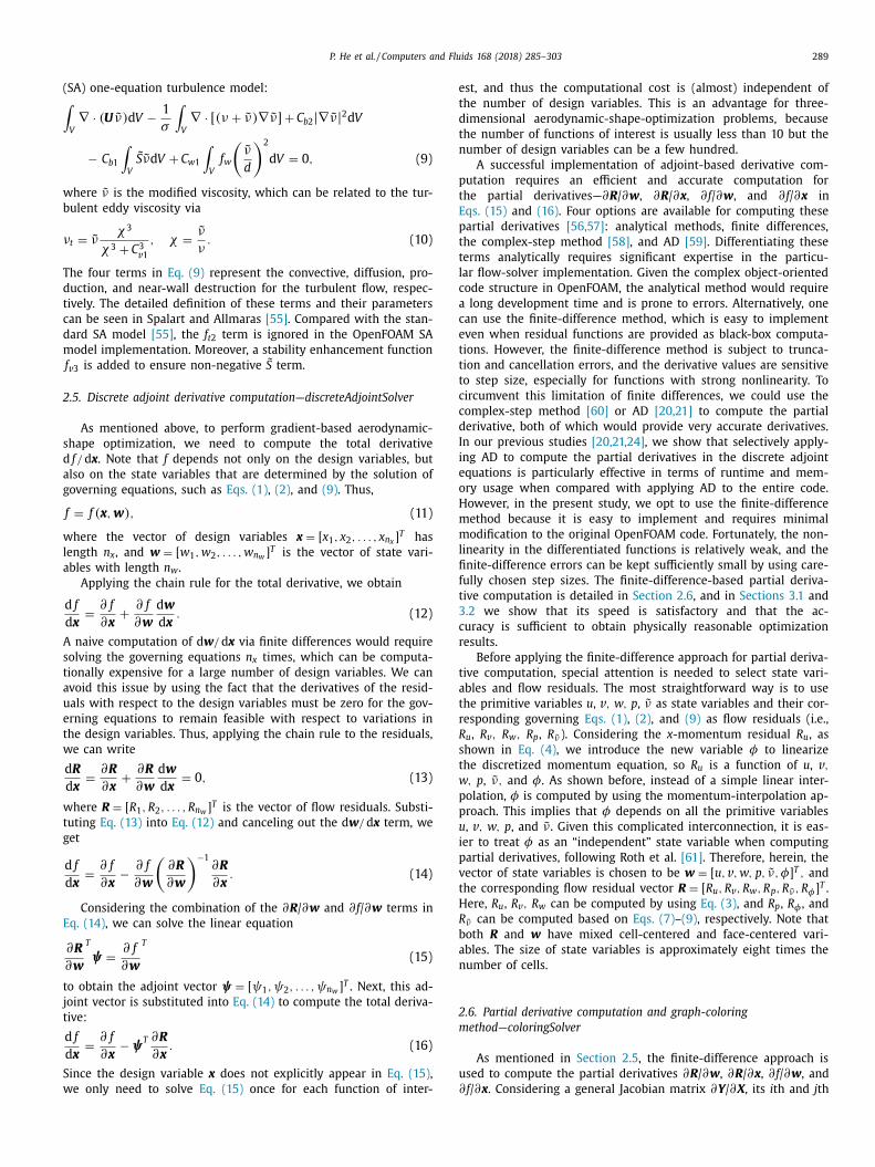
SA) one-equation turbulence model:
V
∇ · ( U ̃ ν)d V − 1
σ
∫ V
∇ · [(ν + ˜ ν) ∇ ̃ ν] + C b2 |∇ ̃ ν| 2 d V
− C b1
∫ V
˜ S ̃ νd V + C w 1
∫ V
f w
(˜ ν
d
)2
d V = 0 , (9)
here ˜ ν is the modified viscosity, which can be related to the tur-
ulent eddy viscosity via
t = ˜ νχ3
χ3 + C 3 v 1 , χ =
˜ ν
ν. (10)
he four terms in Eq. (9) represent the convective, diffusion, pro-
uction, and near-wall destruction for the turbulent flow, respec-
ively. The detailed definition of these terms and their parameters
an be seen in Spalart and Allmaras [55] . Compared with the stan-
ard SA model [55] , the f t 2 term is ignored in the OpenFOAM SA
odel implementation. Moreover, a stability enhancement function
f v 3 is added to ensure non-negative ˜ S term.
.5. Discrete adjoint derivative computation—discreteAdjointSolver
As mentioned above, to perform gradient-based aerodynamic-
hape optimization, we need to compute the total derivative
f/ d x . Note that f depends not only on the design variables, but
lso on the state variables that are determined by the solution of
overning equations, such as Eqs. (1) , (2) , and (9) . Thus,
f = f ( x , w ) , (11)
here the vector of design variables x = [ x 1 , x 2 , . . . , x n x ] T has
ength n x , and w = [ w 1 , w 2 , . . . , w n w ] T is the vector of state vari-
bles with length n w
.
Applying the chain rule for the total derivative, we obtain
d f
d x =
∂ f
∂ x +
∂ f
∂ w
d w
d x . (12)
naive computation of d w / d x via finite differences would require
olving the governing equations n x times, which can be computa-
ionally expensive for a large number of design variables. We can
void this issue by using the fact that the derivatives of the resid-
als with respect to the design variables must be zero for the gov-
rning equations to remain feasible with respect to variations in
he design variables. Thus, applying the chain rule to the residuals,
e can write
d R
d x =
∂ R
∂ x +
∂ R
∂ w
d w
d x = 0 , (13)
here R = [ R 1 , R 2 , . . . , R n w ] T is the vector of flow residuals. Substi-
uting Eq. (13) into Eq. (12) and canceling out the d w / d x term, we
et
d f
d x =
∂ f
∂ x − ∂ f
∂ w
(∂ R
∂ w
)−1 ∂ R
∂ x . (14)
Considering the combination of the ∂ R / ∂ w and ∂ f / ∂ w terms in
q. (14) , we can solve the linear equation
∂ R
∂ w
T
ψ =
∂ f
∂ w
T
(15)
o obtain the adjoint vector ψ = [ ψ 1 , ψ 2 , . . . , ψ n w ] T . Next, this ad-
oint vector is substituted into Eq. (14) to compute the total deriva-
ive:
d f
d x =
∂ f
∂ x − ψ
T ∂ R
∂ x . (16)
ince the design variable x does not explicitly appear in Eq. (15) ,
e only need to solve Eq. (15) once for each function of inter-
st, and thus the computational cost is (almost) independent of
he number of design variables. This is an advantage for three-
imensional aerodynamic-shape-optimization problems, because
he number of functions of interest is usually less than 10 but the
umber of design variables can be a few hundred.
A successful implementation of adjoint-based derivative com-
utation requires an efficient and accurate computation for
he partial derivatives—∂ R / ∂ w , ∂ R / ∂ x , ∂ f / ∂ w , and ∂ f / ∂ x in
qs. (15) and (16) . Four options are available for computing these
artial derivatives [56,57] : analytical methods, finite differences,
he complex-step method [58] , and AD [59] . Differentiating these
erms analytically requires significant expertise in the particu-
ar flow-solver implementation. Given the complex object-oriented
ode structure in OpenFOAM, the analytical method would require
long development time and is prone to errors. Alternatively, one
an use the finite-difference method, which is easy to implement
ven when residual functions are provided as black-box computa-
ions. However, the finite-difference method is subject to trunca-
ion and cancellation errors, and the derivative values are sensitive
o step size, especially for functions with strong nonlinearity. To
ircumvent this limitation of finite differences, we could use the
omplex-step method [60] or AD [20,21] to compute the partial
erivative, both of which would provide very accurate derivatives.
n our previous studies [20,21,24] , we show that selectively apply-
ng AD to compute the partial derivatives in the discrete adjoint
quations is particularly effective in terms of runtime and mem-
ry usage when compared with applying AD to the entire code.
owever, in the present study, we opt to use the finite-difference
ethod because it is easy to implement and requires minimal
odification to the original OpenFOAM code. Fortunately, the non-
inearity in the differentiated functions is relatively weak, and the
nite-difference errors can be kept sufficiently small by using care-
ully chosen step sizes. The finite-difference-based partial deriva-
ive computation is detailed in Section 2.6 , and in Sections 3.1 and
.2 we show that its speed is satisfactory and that the ac-
uracy is sufficient to obtain physically reasonable optimization
esults.
Before applying the finite-difference approach for partial deriva-
ive computation, special attention is needed to select state vari-
bles and flow residuals. The most straightforward way is to use
he primitive variables u , v , w, p , ˜ ν as state variables and their cor-
esponding governing Eqs. (1) , (2) , and (9) as flow residuals (i.e.,
u , R v , R w
, R p , R ˜ ν ). Considering the x -momentum residual R u , as
hown in Eq. (4) , we introduce the new variable φ to linearize
he discretized momentum equation, so R u is a function of u , v ,, p , ˜ ν, and φ. As shown before, instead of a simple linear inter-
olation, φ is computed by using the momentum-interpolation ap-
roach. This implies that φ depends on all the primitive variables
, v , w, p , and ˜ ν . Given this complicated interconnection, it is eas-
er to treat φ as an “independent” state variable when computing
artial derivatives, following Roth et al. [61] . Therefore, herein, the
ector of state variables is chosen to be w = [ u, v , w, p, ̃ ν, φ] T , and
he corresponding flow residual vector R = [ R u , R v , R w
, R p , R ˜ ν , R φ] T .
ere, R u , R v , R w
can be computed by using Eq. (3) , and R p , R φ , and
˜ ν can be computed based on Eqs. (7) –(9) , respectively. Note that
oth R and w have mixed cell-centered and face-centered vari-
bles. The size of state variables is approximately eight times the
umber of cells.
.6. Partial derivative computation and graph-coloring
ethod—coloringSolver
As mentioned in Section 2.5 , the finite-difference approach is
sed to compute the partial derivatives ∂ R / ∂ w , ∂ R / ∂ x , ∂ f / ∂ w , and
f / ∂ x . Considering a general Jacobian matrix ∂ Y / ∂ X , its i th and j th

290 P. He et al. / Computers and Fluids 168 (2018) 285–303
Fig. 3. A 5 × 5 diagonal Jacobian matrix computed with graph coloring. The
columns with the same colors are perturbed simultaneously because they affect
independent sets of rows, resulting in a maximum of three colors in this case. The
dashed line denotes parallel matrix storage in PETSc using two processors.
Table 1
Connectivity level for simpleFoam flow residuals with Spalart–
Allmaras turbulence model. The numbers denote how many levels
of neighboring state variables are connected to a flow residual.
U p ˜ ν φ
R U 2 1 1 0
R p 3 2 2 1
R ˜ ν 1 2 0
R φ 3 2 2 1
fi
u
t
s
h
s
t
i
s
t
t
f
s
w
t
s
s
F
a
m
t
u
i
t
e
m
o
t
p
element can be computed as (∂ Y
∂ X
)i, j
=
Y i ( X + ε e j ) − Y i ( X )
ε , (17)
where the subscripts i and j are the row and column indices of
the matrix, respectively, ε is the finite-difference step, and e j is
a unit vector with unity in row j and zeros in all other rows. A
naive implementation is that we perturb each column of the ma-
trix and compute the corresponding partial derivatives for all rows.
Although evaluating the Y function is relatively cheap, this process
needs to be repeated n C times, where n C is the number of columns
in the Jacobian matrix. This is not a severe issue for ∂ R / ∂ x and
∂ f / ∂ x , because the size of x does not typically exceed a few hun-
dred. However, for ∂ R / ∂ w and ∂ f / ∂ w , the computational cost may
be too high, because the size of w can easily escalate to tens of
millions for a three-dimensional aerodynamic-optimization prob-
lem.
To accelerate the finite-difference-based partial derivative com-
putation, we use a graph-coloring method. The graph-coloring ap-
proach exploits the sparsity of the Jacobian matrix and enables us
to simultaneously perturb multiple columns by perturbing sets of
columns that influence independent sets of rows. Considering the
diagonal Jacobian matrix in Fig. 3 , as mentioned above, a naive
Fig. 4. Example of sparsity pattern for ∂ R / ∂ w , generated based on a curved cube geome
subscripts denote the cell or face index where n c and n f are the total number of cells
Similar ordering is also applied to R . (a) Structured hexahedral mesh (cell size: 100, face
(cell size: 94, face size: 345, Jacobian row size: 815).
nite-difference im plementation would require five function eval-
ations. To accelerate this process, we partition all the columns of
he matrix into different structurally orthogonal subgroups (colors),
uch that, in one structurally orthogonal subgroup, no two columns
ave a nonzero entry in a common row. The columns with the
ame colors are perturbed simultaneously and the number of func-
ion evaluations can be reduced to three.
The actual ∂ R / ∂ w sparsity pattern for a three-dimensional case
s obviously much more complicated than the diagonal matrix
hown in Fig. 3 . Table 1 summarizes the level of connectivity for
he simpleFoam flow residuals. Depending on the mesh topology,
he number of connected state variables for a flow residual differs
rom case to case, although their connectivity levels remain the
ame. As an example, Fig. 4 shows the sparsity pattern for ∂ R / ∂ w ,
hich is generated based on the connectivity level and mesh
opology information from a curved cube geometry. We show re-
ults for both a structured hexahedral mesh and an unstructured
nappy hexahedral mesh which is generated by the built-in Open-
OAM mesh tool snappyHexMesh. Given that we mix cell-centered
nd face-centered variables and residuals, we use a state-by-state
atrix ordering because it is straightforward to implement. Note
hat we reorder the state Jacobian matrix to reduce the memory
sage for the adjoint-equation solution (see Section 2.7 ). As shown
n Fig. 4 , the p and φ residuals have the largest level of connec-
ivity and therefore denser rows. Also, while the structured mesh
xhibits a block-diagonal structure, the unstructured mesh is much
ore irregular. Therefore, an analytical determination of the col-
ring, such as that described by Lyu et al. [21] , is impossible for
he unstructured mesh ∂ R / ∂ w , and an efficient coloring scheme to
artition the Jacobian matrices is needed.
try. We use a state-by-state matrix ordering (i.e., w = [ U 1: n c , p 1: n c , ̃ ν1: n c , φ1: n f ] ). The
and faces, respectively. For example, U 1: n c = [ u 1 , v 1 , w 1 , u 2 , v 2 , w 2 , . . . , u n c , v n c , w n c ] .
size: 365, Jacobian row size: 865) and (b) unstructured snappy hexahedral mesh

P. He et al. / Computers and Fluids 168 (2018) 285–303 291
Algorithm 1 Parallel graph coloring for sparse Jacobian matrix J .
Input: Jacobian matrix: J � Global size: n R × n C Output: Graph-coloring vector: G � Global size: 1 × n C
1: G j ← −1 for each j ∈ C all � Label all columns as uncolored ( −1 )
2: R j ← rand for each j ∈ C all � Initialize conflict-resolution vector with random numbers
3: for t ∈ { interior , global } do � Color interior columns first and then global columns
4: for n ∈ { 0 , . . . , ∞} do � n : current color
5: G j ← n for each j ∈ C uncolored � Assign current color n to uncolored columns
6: for r ∈ R local do � R local : Local rows owned by the current processor
7: S = F (t, n, R, G, J i = r, j∈ C nonzeros ) � S: reset columns. F : conflict-resolution function
8: G j ← −1 for each j ∈ S � Reset these columns as uncolored
9: if t = interior and G j � = −1 for each j ∈ C interior then
10: break � All interior columns are colored
11: else if t = global and G j � = −1 for each j ∈ C global then
12: break � All global columns are colored
Algorithm 2 Conflict-resolution function for graph coloring.
Input: Task to resolve: t , current color: n , conflict-resolution vector: R , graph-coloring vector: G , and nonzero elements in a given row:
J i = r, j∈ C nonzeros
Output: Columns to reset: S
1: function S = F ( t, n, R, G, J i = r, j∈ C nonzeros )
2: if t = interior then
3: v min ← min (R j ) for each j ∈ C interior ∪ C local
4: j min ← find_index (R = v min ) � Find column index with minimal R value
5: for j ∈ { C interior , C local } do
6: if G j = n and j � = j min then
7: S.append( j) � Append all columns but j min to S for current color n
8: if t = global then
9: for range ∈ { local , global } do
10: ˆ G ← G
k for each k ∈ all processors � Gather all colors to current processor
11: v min ← min (R j ) for each j ∈ C range
12: j min ← find _ index (R = v min )
13: for j ∈ C range do
14: if j ∈ C interior then
15: S.append( j / ∈ C interior ) � Always keep interior columns
16: else if ˆ G j = n and j � = j min then
17: S.append( j)
p
v
(
(
j
t
o
b
p
t
i
c
o
c
t
n
i
J
g
c
t
e
o
f
(
c
d
c
i
t
a
c
w
b
a
n
(
n
p
a
o
H
a
i
i
a
f
The idea of partitioning the Jacobian matrix was initially pro-
osed by Curtis et al. [62] . This process was then modeled as
arious graph-coloring problems, such as the column intersection
distance-1) graph proposed by Coleman et al. [63] and bipartite
distance-2) graph introduced by Gebremedhin et al. [64] . The ob-
ective is to find the fewest colors possible for a given Jacobian ma-
rix. Note that this number is bounded by the maximum number
f nonzero entries in a row of the Jacobian. Unfortunately, it has
een shown that the graph-coloring computation is an NP-hard
roblem [63] ; it is very unlikely that a universal algorithm exists
o determine the fewest possible colors in polynomial time. This
ssue becomes even more challenging if one needs to extend the
oloring algorithm for parallel computation in a distributed mem-
ry system. For example, Nielsen and Kleb [60] used the greedy
oloring algorithm [62] to accelerate state Jacobian computation in
heir adjoint implementation, which resulted in a reasonably small
umber of colors. However, the greedy algorithm is known to be
nherently sequential and is difficult to parallelize for tackling large
acobian matrices [65] . Given this background, a heuristic parallel
raph-coloring algorithm is proposed herein.
The general idea of heuristic graph coloring is to tentatively
olor and then resolve any conflict. The pseudo-algorithm is de-
ailed in Algorithm 1 . More specifically, there is a loop over
ach row that assigns a tentative color to all nonzero, uncol-
red columns ( Algorithm 1 , lines 4–6). Next, a conflict-resolution
unction is called to determine the “winner” column in this row
Algorithm 1 , line 7), and all the other columns are reset to “un-
olored” ( Algorithm 1 , line 8). The conflict-resolution function is
etailed in Algorithm 2 . The above process is repeated until all
olumns are colored ( Algorithm 1 , lines 9–12). This general idea
s similar to that described by Bozda ̆g et al. [66] . The challenge is
hat the operations above need to be fully parallel and scalable. In
ddition, the number of colors should be independent of the Ja-
obian sizes and the number of CPU cores. To achieve these goals,
e developed an improved parallel algorithm to tackle the Jaco-
ian matrix with O(10 million) rows using O(10 0 0) CPU cores. This
lgorithm is optimized based on the parallel storage and commu-
ication architecture of PETSc, and it consists of two major steps
i.e., interior and global; see Algorithm 1 , line 3).
First, we color the interior columns that do not share any
onzero entry in a common column among the distributed CPU
rocessors. As mentioned before, the PETSc library is used to store
nd manipulate the large sparse matrices and vectors. An example
f the PETSc’s parallel matrix storage strategy is shown in Fig. 3 .
ere each processor owns different portions or rows of the matrix,
nd a similar parallel storage is also used for vectors. As shown
n Fig. 3 , column 0 is interior for Proc0 and columns 3 and 4 are
nterior for Proc1. These interior columns can be safely colored on
local processor without a conflict between processors. Note that,
or each processor, we only color the columns in diagonal blocks to

292 P. He et al. / Computers and Fluids 168 (2018) 285–303
v
p(
w
s
b
s
a
t
l
t
∂
v
t
t
u
t
W
s
2
w
m
f
t
J
d
t
s
i
p
m
p
s
b
m
fi
d
v
t
v
2
o
S
T
(
S
o
t
t
i
s
t
p
t
o
avoid any message-passing interface (MPI) communication at this
step ( Algorithm 1 , line 6). Next, we repeat the above coloring strat-
egy for global columns, whereas the colored interior columns re-
main untouched. Note that we need the coloring information from
other processors, and MPI communications are needed at this step.
To ensure a successful coloring process, a robust conflict-resolution
function is needed. To explore the potential for a smaller number
of colors, the “winner” of each conflicting column is determined in
a random manner ( Algorithm 1 , line 2). Note that, when determin-
ing the winner for global columns, we need to first complete the
coloring for local columns to prevent deadlock ( Algorithm 2 , line
9).
In this paper, we use the graph-coloring scheme detailed above
to accelerate the computation of the partial derivative for both
∂ R / ∂ w and ∂ f / ∂ w . Special attention is needed for the ∂ f / ∂ w col-
oring scheme. Typically, f is computed based on the integration
of state variables over a surface (e.g., drag and lift). From a dis-
crete perspective, this implies that the number of connected states
for f is on the order of N D (the total number of cell faces on the
surface). To enable the coloring scheme for ∂ f / ∂ w , we divide f
into N D different cell faces. In other words, ∂ f/∂ w =
∑ N D i =1
∂ f i /∂ w .
With this treatment, we can easily obtain the connectivity for each
f i / ∂w , compute the coloring, calculate the partial derivatives, and
sum their values to the final ∂ f / ∂ w matrix. We observe that the
number of colors for ∂ f / ∂ w is typically one order of magnitude less
than the number of colors for ∂ R / ∂ w . Therefore, in Section 3.1 , we
mainly focus on evaluating the performance of the coloring scheme
for ∂ R / ∂ w .
No coloring scheme is needed for ∂ R / ∂ x and ∂ f / ∂ x . Instead,
a brute-force finite-difference approach is used: We first perturb
each design variable and deform the surface and volume meshes to
compute the mesh-deformation derivative matrix ( d x v / d x , where
x v is the volume-mesh coordinates) in the Python layer. As men-
tioned in Section 2.3 , this operation requires less than 0.1% of the
CFD simulation time. This matrix is then passed to the adjoint
solver, which allows us to directly compute ∂ R / ∂ x and ∂ f / ∂ x . Note
that the number of operations for computing ∂ R / ∂ x and ∂ f / ∂ x is
proportional to the number of design variables, which does not
typically exceed a few hundred. Finally, we observe that the first-
order forward-differencing scheme is the most efficient and robust
option, so we use it to compute all partial derivatives in this paper.
2.7. Solution of adjoint equations
Adjoint derivative computation requires a robust linear-
equation solver, especially for realistic geometry configurations
with highly complex flow conditions [30,67–69] . We use the PETSc
library to solve the linear equation shown in Eq. (15) . PETSc
provides a wide range of parallel linear- and nonlinear-equation
solvers with various preconditioning options. We use the gener-
alized minimal residual (GMRES) iterative linear-equation solver
with the additive Schwartz method as the global preconditioner.
For the local preconditioning, we use the incomplete lower and
upper (ILU) factorization approach with one or two levels of fill-
in. This strategy is effective for solving the adjoint equation, as re-
ported in previous studies [21,24] . To reduce the memory usage
of ILU fill, we adopt the nested-dissection matrix-reordering ap-
proach. The preconditioning matrix is computed by using a color-
ing approach similar to that used in Section 2.6 , except that we use
the first-order upwind scheme to compute the convective terms of
flow residuals. Since we have a mix of cell- and face-centered state
variables and flow residuals, and their magnitudes are quite differ-
ent (e.g., the magnitudes of U and φ), we need to scale all the par-
tial derivatives so that their magnitudes are as similar as possible.
By properly scaling the Jacobian matrix, the diagonal dominance
and condition number can be improved, thus improving the con-
ergence of the linear equations. The scaled finite-difference com-
utation for the state Jacobian matrix takes the form
∂ R
∂ W
)scaled
i, j
=
C R i
R i ( W + C W
j ε e j ) − C R
i R i ( W )
ε , (18)
here C R and C W are the scaling factors for the residuals and
tates, respectively. For the cell-centered residuals, C R is chosen to
e the cell volume whereas, for the face-centered residuals, C R is
et to be the face area S f . The state scaling factors C W for U , p , ˜ ν,
nd φ are selected to be U 0 , U
2 0 / 2 , ˜ ν0 , and U 0 S f , respectively. Here
he subscript 0 denotes the inlet (far-field) reference value. Simi-
ar scaling is also applied to ∂ f / ∂ W , ∂ R / ∂ x , and ∂ f / ∂ x . Note that
he scaling is only applied when computing the partial derivatives
R / ∂ w , ∂ f / ∂ w , ∂ R / ∂ x , and ∂ f / ∂ w , whereas the values of the state
ariables are unchanged, which ensures a consistent dimension for
he flow solver because OpenFOAM uses dimensional variables for
he flow solution. Also note that the scaled partial derivative val-
es differ from their original values. However, it is straightforward
o prove that the final values of the total derivative are the same.
e observe that the convergence of the adjoint equation can be
ignificantly improved by using the above scaling of R and w .
.8. Constrained nonlinear optimization—pyOptSparse
We set up our optimization problems by using pyOptSparse,
hich is an open source, object-oriented Python interface for for-
ulating constrained nonlinear optimization problems. This inter-
ace is based on the original pyOpt [32] module but includes ex-
ensive modifications to facilitate the assembly of sparse constraint
acobians. pyOptSparse provides a high-level API for defining the
esign variables, the objective function, and the constraint func-
ions. pyOptSparse itself does not include optimization problem
olvers, but it provides interfaces for several optimization packages,
ncluding some open source packages.
In this study, we use SNOPT [48] to solve the optimization
roblems. SNOPT implements the sequential quadratic program-
ing algorithm to solve the constrained nonlinear optimization
roblem and uses the quasi-Newton method to solve the quadratic
ubproblem, where the Hessian of the Lagrangian is approximated
y using a Broyden–Fletcher–Goldfarb–Shanno update. The opti-
ality in SNOPT is quantified by the norm of the residual of the
rst-order Karush–Kuhn–Tucker optimality conditions [48,70] .
As with all gradient-based optimizers, SNOPT requires the
erivatives of objective and constraints with respect to all design
ariables for each optimization iteration. We compute these deriva-
ives efficiently and accurately by using the adjoint approach de-
eloped herein.
.9. Code structure and implementation
The adjoint derivative computation is a key module in
ur optimization framework. We developed a new class called
IMPLEDerivativeClass based on the OpenFOAM framework.
his class contains all the functions for the coloring solver
coloringSolver) and the discrete adjoint solver (discreteAdjoint-
olver), including the connectivity computation, parallel graph col-
ring, partial derivative computation, and adjoint-equation solu-
ion. Fig. 5 shows the code structure and calling sequence for
hese two solvers. Note that we only need to run the color-
ng solver once per optimization, and the coloring information is
aved. The discreteAdjointSolver then reads the coloring informa-
ion as input when computing ∂ R / ∂ w and ∂ f / ∂ w . As an exam-
le, Fig. 6 shows the code structure for the ComputedRdW func-
ion. Here, we first compute the reference flow residuals based
n the unperturbed, converged flow solutions. Next, we start from

P. He et al. / Computers and Fluids 168 (2018) 285–303 293
Fig. 5. Code structure for coloring and discrete adjoint solvers.
Fig. 6. Code structure for state Jacobian matrix ( ∂ R / ∂ w ) computation function.
t
s
fl
i
t
m
u
m
p
a
t
Us
b
j
i
p
d
s
a
i
a
s
H
i
a
p
3
t
a
d
m
f
T
w
t
m
a
t
3
a
r
r
p
b
r
s
w
1
i
d
e
r
h
h
a
b
c
m
o
t
c
r
n
a
a
a
b
m
he first color and simultaneously perturb the state variables as-
ociated with it. Based on the perturbed flow solutions, new
ow residuals are computed, and the finite-difference approach
s used to compute partial derivatives. Finally, we assign the par-
ial derivative values for the ∂ R / ∂ w matrix stored in PETSc for-
at and reset the perturbations. The above process is repeated
ntil all the colors are done. Note that the boundary conditions
ust be updated for each state-variable perturbation. For exam-
le, when we perturb the velocity of a cell immediately next to
n interprocessor boundary patch, we need to interpolate the per-
urbed velocity onto this boundary patch. This is done by calling
.correctBoundaryConditions() in OpenFOAM. We need
imilar updates for all flow variables. Note that updating the
oundary condition is essential for accurately computing the ad-
oint derivative.
One of the advantages of the discrete adjoint approach is that
ts formulation starts from the discretized NS equations, and the
roperties of flow solver (e.g., the flow convergence behavior and
erivatives) are preserved. Following this idea, we reuse the code
tructure in the simpleFoam flow solver as much as possible in the
djoint implementation. This not only facilitates the adjoint code
mplementation but also reduces the effort required to modify the
djoint code when the flow solver is updated. Listing 1 shows a
ample function for computing the momentum-equation residuals.
ere we reuse the fvm matrix ( UEqn ; the left-hand-side matrix)
mplemented in the original simpleFoam flow solver and calculate
matrix-vector product for residual computations. A similar im-
lementation is used to compute other flow residuals.
. Results and discussion
We now evaluate the performance of adjoint derivative compu-
ation in terms of speed, scalability, and accuracy. We then perform
basic optimization of a simple bluff body geometry along with
etailed flow analyses and experimental validation of the opti-
ization result. In addition, we apply the optimization framework
or two more complex cases: UAV and car aerodynamic design.
he main objective of this section is to demonstrate our frame-
ork’s capabilities for various constrained-optimization applica-
ions. A comprehensive optimization study (e.g., multipoint opti-
ization [29,71] and mesh-refinement studies) for each of these
pplications is outside the present scope and will be done in fu-
ure work.
.1. Performance evaluation
To evaluate the performance of our adjoint framework, we use
simple bluff geometry—the Ahmed body. The Ahmed body is a
ectangular block geometry with a rounded front end and a sharp
amp near the rear end, as shown in Fig. 2 (a). It was originally
roposed and tested by Ahmed et al. [49] in 1984 and has since
een widely used as a CFD benchmark. Here we choose the 25 °amp-angle configuration as our baseline geometry.
Only half of the body is simulated, and the simulation domain
ize is 8 L , 2 L , and 2 L in the x , y , and z directions, respectively,
here L is the length of Ahmed body. The Reynolds number is
.4 × 10 6 based on L and U 0 . A second-order linear upwind scheme
s used to differentiate the divergence terms, whereas the central
ifferential scheme is adopted for the diffusion terms. This differ-
ntiation configuration is reportedly the most efficient and accu-
ate for RANS simulations [6] and is used for all the simulations
erein.
For the derivative computation, the unstructured snappy hexa-
edral mesh is generated with approximately 1 million cells. The
veraged y + is 60, so a wall function is used for νt . For the scala-
ility test, we generate meshes with up to 10 million cells. For the
oloring scheme, we also show results for a structured hexahedral
esh for comparison. All test simulations in this section were done
n Stampede 2, which is a high-performance computing (HPC) sys-
em equipped with a second generation Intel Xeon Phi 7250 Pro-
essor: Knights Landing (KNL). Each KNL node has 68 CPU cores
unning at 1.4 GHz and 96 GB of DDR4 memory, and they are con-
ected through the Sandy Bridge FDR Infiniband. Stampede 2 has
peak PFLOPS of 18. The OpenFOAM and PETSc versions are 2.4.x
nd 2.7.6, respectively, and they were compiled with Intel-17.0.4
nd IMPI-17.0.3.
We first test the scalability for the coloring solver by using
oth structured hexahedral and unstructured snappy hexahedral
eshes, as shown in Fig. 7 . The Jacobian row sizes are 8.8 × 10 6

294 P. He et al. / Computers and Fluids 168 (2018) 285–303
Listing 1. Sample function for computing momentum residuals. This sample code just illustrates the idea of reusing simpleFoam code (i.e., the fvm matrix UEqn ) for residual
computation; the actual computeURes function in our code is slightly different.
Fig. 7. Performance of parallel coloring scheme for state Jacobian matrix ∂ R / ∂ w .
The coloring runtime scales up to 10 million cells and 1024 CPU cores, and the
number of colors is almost independent of the mesh size and the number of CPU
cores.
a
r
l
c
c
r
c
s
t
s
I
[
o
i
t
f
o
e
h
h
c
C
A
c
T
c
b
s
fl
nd 8.4 × 10 7 for 1 million and 10 million cells, respectively. The
untime for parallel coloring computation scales well up to 10 mil-
ion mesh cells and 1024 CPU cores. In addition, the number of
olors is almost independent of Jacobian size and number of CPU
ores, which confirms the efficiency of our parallel coloring algo-
ithm. In terms of mesh topology, the number of structured mesh
olors ( ∼ 1300) is generally less than the number of unstructured
nappy mesh colors ( ∼ 2300) because the stencil for the unstruc-
ured snappy mesh is much larger than the structured mesh, re-
ulting in a denser Jacobian matrix and therefore more colors.
n the previous adjoint coloring implementations using analytical
21] , greedy [60] , or heuristic [72] approaches, the number of col-
rs was reported to be O(100), which is much less than in our
mplementation. This is primarily due to the level-three connec-
ivity, as shown in Table 1 , and especially to the inclusion of the
ace-center state variable φ in our adjoint formulation. As a result,
ur Jacobian matrix is relatively dense: a maximum of 307 nonzero
ntries are in a row of the state Jacobian for the structured hexa-
edral mesh and 811 nonzero entries for the unstructured snappy
exahedral mesh.
Next, we evaluate the speed and scalability of adjoint derivative
omputation in Fig. 8 . The objective function is the drag coefficient
D , defined as C D = D/ 0 . 5 ρU
2 0 A ref , where D is the drag force and
ref is the frontal area of the Ahmed body. The adjoint derivative
omputation scales well up to 10 million cells and 1024 CPU cores.
his good scalability is primarily due to the performance of the
oloring solver, as shown in Fig. 7 . Here, we also show the scala-
ility of flow simulation for reference. The derivative computation
cales as well as does the flow simulation.
In terms of speed, the derivative computation is faster than the
ow solution for 10 million cells, whereas for 1 million cells, the

P. He et al. / Computers and Fluids 168 (2018) 285–303 295
Fig. 8. Scalability of flow and adjoint computations. The adjoint runtime scales up
to 10 million cells and 1024 CPU cores.
Table 2
Runtimes of flow and adjoint computation for increasing number
of CPU cores. The adjoint-flow runtime ratio is of order unity.
1 million cells
KNL nodes 2 2 2 2
CPU cores 16 32 64 128
Flow runtime (s) 6418 3593 2039 1377
Adjoint runtime (s) 7036 3686 1955 1331
Adjoint-flow runtime ratio 1.10 1.03 0.96 0.97
10 million cells
KNL nodes 24 24 32 32
CPU cores 128 256 512 1024
Flow runtime (s) 14543 7539 3677 2709
Adjoint runtime (s) 12763 6037 3494 2412
Adjoint-flow runtime ratio 0.88 0.80 0.95 0.89
Table 3
Adjoint computational-time breakdown for Ahmed body. Computation
of ∂ R / ∂ w , ∂ R / ∂ w (PC), and the solution of the adjoint equation are the
most expensive whereas the computational cost for ∂ f / ∂ w , ∂ R / ∂ x , and
∂ f / ∂ x is very small. PC stands for “preconditioning matrix computation.”
Runtime (s) Percent
∂ R / ∂ w 547 .0 41 .1%
∂ R / ∂ w (PC) 425 .9 32 .0%
∂ f / ∂ w 2 .7 0 .2%
∂ R / ∂ x 5 .3 0 .4%
∂ f / ∂ x 2 .7 0 .2%
Adjoint equation 347 .4 26 .1%
a
l
3
b
m
s
6
t
a
t
s
i
T
c
C
Fig. 9. Convergence history of flow and adjoint residuals for Ahmed-body case with
1 million unstructured snappy hexahedral cells.
p
t
i
T
a
t
2
m
o
t
p
w
o
i
m
t
n
m
2
t
t
c
n
i
0
C
p
d
t
(
p
i
a
t
djoint computation speed is very close to that of the flow simu-
ation and outperforms the flow simulation when using more than
2 CPU cores. The faster derivative computation for greater num-
er of cells is primarily attributed to the fact that the flow requires
ore iterations to converge. The convergence tolerance of the flow
olver is set to 10 −8 , and the 1- and 10-million-cell cases require
0 0 0 and 80 0 0 steps to converge, respectively.
Overall, the runtime ratio between the adjoint and flow compu-
ation is of order unity, independent of Jacobian size (mesh cells)
nd number of CPU cores, as shown in Table 2 . This confirms
he efficiency of the adjoint derivative computation. Moreover, the
calability test for the flow and adjoint indicates that good scalabil-
ty is achieved if each CPU core owns no fewer than 20 0 0 0 cells.
able 3 shows the detailed runtime breakdown for the derivative
omputation using the 1-million-cell Ahmed-body case with 128
PU cores. Computing the state Jacobian matrix is the most ex-
ensive part, followed by computing the state Jacobian precondi-
ioning matrix. Note that the cost of computing the state Jacobian
s proportional to n c T resid , where n c is the number of colors and
resid is the cost of one flow residual computation. Meanwhile, the
djoint equation converges in about 500 iterations (see Fig. 9 ) and
akes 26.1% of the total adjoint runtime.
In terms of peak resident memory, the flow solutions require
.9 and 25.2 GB for the 1-million-cell (16 CPU cores) and 10-
illion-cell (128 CPU cores) cases, respectively, whereas the mem-
ry requirement rapidly grows to 101.8 and 886.1 GB to compute
he adjoint derivative for 1 and 10 million cells, respectively. The
eak memory usage happens at the adjoint-equation solution step
hen the ILU preconditioner is filled in. This relatively large mem-
ry requirement indicates that our discrete adjoint implementation
s memory bound. Fortunately, current HPC systems typically have
ore than 64 GB of memory per node, which alleviates this limi-
ation. As mentioned above, Stampede 2 has 96 GB of memory per
ode, and we require at least 2 and 10 nodes for the 1- and 10-
illion-cell cases, respectively. To be conservative, we use at least
4 nodes in practice for the 10 million runs (see Table 2 ). Note
hat a KNL node has many more CPU cores than traditional sys-
ems, but the processors run at lower frequencies. Therefore, when
omparing the speed of KNL against traditional CPUs, a node-to-
ode comparison is more appropriate than a core-to-core compar-
son. For example, a combined flow and adjoint computation takes
.8 hours for the 1 million cells when using 2 KNL nodes with 128
PU cores (see Table 2 ).
Finally, we evaluate the accuracy of the adjoint derivative com-
utation by using the derivative computed directly from the finite-
ifference approach as a reference. The verification of the deriva-
ive of the drag coefficient with respect to the far-field velocity
d C D / d u 0 ) is shown in Table 4 . Because the finite-difference ap-
roach is used to compute the partial derivatives in the adjoint
mplementation, the impact of the finite-difference step size on the
ccuracy is shown for comparison. The step size used in the par-
ial derivative computations is defined in Eq. (18) . Note that, for

296 P. He et al. / Computers and Fluids 168 (2018) 285–303
Table 4
Verification of adjoint derivative computation for d C D / d u 0 , where u 0 is the far-field velocity in the x direction. For a step size of 10 −8 , the
adjoint derivative matches the reference value to the fifth digit.
Table 5
Verification of adjoint derivative computation for d C D / d x , where x =
(x 0 , x 1 , x 2 , x 3 ) is the FFD design variable vector. The average error is less
than 0.1%.
Fig. 10. Optimization of ramp angle for Ahmed-body case. The optimization con-
verges to the optimum in only four iterations.
Fig. 11. Convergence history of C D and optimality for optimizing Ahmed-body ramp
shape. Drag reduction is 9.4%. The optimization results are validated by wind tunnel
experiments.
1
t
r
o
d
t
c
u
m
s
u
o
the scaled partial derivatives, the actual perturbation is the step
size multiplied by the scaling factor ( C W ε). The best agreement
occurs for a step size of 10 −8 , for which the adjoint derivative
matches the reference value to the fifth digit. Note that similar
step-size studies are conducted for the reference derivative value
in Table 4 (central difference with a step size of 10 −5 ), and for all
other results shown later in this paper. We find that the errors in
reference derivative values under different finite-differencing step
sizes are much smaller than the errors of adjoint derivative compu-
tation; we thus conclude that using the finite-difference derivatives
as references is reasonable. In addition to the far-field velocity, we
evaluate the accuracy of the derivative with respect to the FFD de-
sign variables ( d C D / d x ), shown in Table 5 , where the design vari-
ables are four FFD points covering the Ahmed-body ramp. Again,
the reference derivative is computed by using the finite-difference
approach. For the best-case scenario ( d C D / d x 1 ), the error is less
than 0.01%, whereas for the worst case ( d C D / d x 3 ), the error is no
more than 0.3%. Overall, the average error is less than 0.1%. The
derivative accuracy from our discrete adjoint implementation suf-
fices for numerical optimization, as shown in Section 3.2 .
3.2. Aerodynamic-shape optimization of Ahmed body
In this section, we optimize the aerodynamic shape of the
Ahmed body. Here we choose the 25 ° ramp-angle configuration
with 1 million cells as our baseline case. This simple geometry
allows us to demonstrate the basic optimization capability and
to verify the optimization framework. Moreover, extensive exper-
imental results are available for Ahmed body, which provide a bet-
ter understanding of the flow fields and optimization results.
First, a single design variable—the ramp angle—is optimized to
verify our adjoint framework. As reported in the original Ahmed-
body experiment [49] , reducing the ramp angle decreases the
ramp-surface contribution to the drag; however, the contribution
from the vertical rear-end surface increases. Thus, an optimal ramp
angle between 0 ° and 40 ° minimizes the drag. This trend is repro-
duced by our CFD simulations (shown in Fig. 10 as the black line).
Here, we perform CFD simulations for ramp angles ranging from 0 °to 30 ° in 5 ° increments. As mentioned in Section 2.2 , the ramp an-
gle is controlled by using global shape control to move a set of FFD
points together, while keeping the upper edge of the ramp fixed.
The result indicates that the optimal ramp angle is approximately
5 °. Next, we conduct an adjoint optimization for drag minimiza-
ion, starting from the 25 ° ramp angle; the result is shown as the
ed dots in Fig. 10 . The optimization converges to the optimum in
nly four iterations.
We next optimize an aerodynamic shape with multiple local
esign variables, as described in Table 6 . We set 25 FFD points on
he ramp surface, forcing the top edge of the ramp to remain un-
hanged. The FFD volume and points are shown in Fig. 2 . We set
p five linear constraints to force the y -direction slope at the sym-
etry plane to remain zero. In addition, we only allow the ramp
urface to move upward, resulting in a shape that is easier to man-
facture for wind tunnel experiments.
Fig. 11 shows the convergence history of C D and optimality for
ptimizing the Ahmed-body ramp shape. Both C and optimality
D
P. He et al. / Computers and Fluids 168 (2018) 285–303 297
Table 6
Ahmed-body ramp-shape optimization problem.
Function or variable Description Quantity
Minimize C D Drag coefficient
with respect to z z coordinate of FFD points 25
subject to g sym y = 0 y direction slope at the symmetry plane is zero 5
0 m < z < 0.1 m Design variable bounds
Fig. 12. Pressure-coefficient contours for baseline and optimized Ahmed-body geometries. The transparent gray area denotes the isosurface of the Q criterion ( Q = 10 0 0 ).
The optimized ramp shape provides better pressure recovery by modifying the rear-end vortex structure and the flow separation on the ramp.
c
b
p
s
o
o
s
(
c
2
t
r
d
m
s
s
t
p
[
a
r
l
o
a
r
i
Q
w
l
d
t
a
s
a
n
p
r
v
r
t
i
l
n
a
a
t
m
e
t
(
t
t
l
fi
o
a
onverge in 23 iterations. The simulated drag coefficient for the
aseline Ahmed body ( C 0 D
) is 0.310, which is 3.4% less than the ex-
erimental result (0.321) at the same Reynolds number [73] . We
peculate that this lower C D value is partially due to the exclusion
f four supporting legs in our simulations. For the optimized ge-
metry, C D drops to 0.281—a 9.4% reduction in drag. In terms of
peed, the optimization takes 24 hours when using 32 CPU cores
Intel Xeon E5-2680 v3 at 2.5 GHz). In total, we perform 24 adjoint
omputations and 29 flow solutions for the optimization. There are
361 colors for the state Jacobian.
To further validate the optimization results, we conducted wind
unnel experiments using the intermediate and final Ahmed body
amp shapes during the optimization. The reduction in drag pre-
icted by our numerical optimization agrees well with the experi-
ental data, as shown in Fig. 11 ; the difference is 0.6% for the final
hape.
Finally, we analyze the flow fields to better understand the re-
ults of optimization. For flows over bluff bodies, the flow separa-
ion near the rear end provides the major contribution to drag; the
ressure drag dominates and the friction drag is relatively small
49] . Therefore, maintaining a favorable pressure distribution (i.e.,
n effective pressure recovery near the rear end) is critical for drag
eduction. Fig. 12 shows the pressure coefficient contours for base-
ine and optimized Ahmed bodies. Although we only simulate and
ptimize half of the Ahmed body, we show the full geometry for
better illustration. We also show the isosurface of the Q crite-
ion, which is a useful metric to identify the vortex structure and
s defined as
=
1
(�i, j �i, j − S i, j S i, j ) , (19)
2here � and S are the rotation and strain rates, respectively. A
arge positive Q implies that the rotational motion of the fluid
ominates its strain (expanding, shrinking, or shearing) motion. For
he baseline geometry, a low-pressure region appears near the top
nd side edges of the ramp surface, matching the experimental ob-
ervation reported by Lienhart and Becker [74, Fig. 12] . Moreover,
distinct vortex structure appears in the simulation results: A cor-
er vortex originates from the top corner of the ramp surface and
ropagates downstream. In addition, strong vorticity occurs on the
amp surface, implying a mild flow separation. Also, behind the
ertical rear-end surface, two counter-rotating vortices form as a
esult of flow recirculation. The simulated vortex structure qualita-
ively agrees with the results observed in Ahmed’s original exper-
ments [49, Figs. 6 and 10] . This vortex structure is closely corre-
ated with the pressure distribution, i.e., the low-pressure regions
ear the side edge and top edge are impacted by the corner vortex
nd the mild flow separation on the ramp, respectively.
Keeping the above baseline-flow structure in mind, we now ex-
mine the pressure distribution over the optimized shape. We find
hat the pressure distribution changes significantly. For the opti-
ized geometry, the low-pressure regions near the top and side
dges shrink, and a high-pressure region emerges in the middle of
he ramp surface. By taking a close look at the optimized shape
top-right corner in Fig. 12 ), we see a bump near the side edge of
he ramp. This bump raises the corner vortex and reduces its in-
ensity, as shown by the Q isosurface in Fig. 12 . As a result, the
ow-pressure region near the side edge is reduced. In addition, we
nd that the local ramp angle near the top edge is reduced in the
ptimized shape ( Fig. 13 ), resulting in a weaker flow separation
nd higher pressure in the middle of the ramp surface. Note that

298 P. He et al. / Computers and Fluids 168 (2018) 285–303
Fig. 13. Ramp shape at symmetry plane and C p profiles on ramp and vertical rear-
end surfaces. The C p profiles are based on the pressure averaged over the lateral
( y ) direction. The pressure increases significantly on the ramp surface, which con-
tributes to the reduced drag.
Fig. 15. Convergence history of C D and optimality for optimizing UAV wing shape.
Drag is reduced by 5.6%.
s
a
a
C
a
m
c
w
t
a
p
w
m
(
this pressure increase, due to better pressure recovery, provides
the major contribution to drag reduction. This conclusion is further
confirmed by the pressure-coefficient profiles at the ramp and ver-
tical rear-end surfaces of the Ahmed body, as shown in Fig. 13 . The
pressure on the ramp surface significantly increases, although the
pressure on the vertical rear-end surface is slightly reduced.
For this section, we verified the adjoint optimization framework
by optimizing with respect to a single design variable (ramp angle).
We then optimized the local shape for the ramp surface and val-
idated the optimization results experimentally. Moreover, we ana-
lyzed the flow in detail to confirm that the result of optimization
is physically reasonable. In the next section, we apply this adjoint
framework to two more complex applications: the aerodynamic-
shape optimization of a UAV and of a car.
3.3. Aerodynamic-shape optimization of unmanned aerial vehicle
Compared with full-size piloted aircraft, UAVs have the ad-
vantage of lower cost, longer endurance, and more flexibility
with respect to the operating environment. Over the last few
years, UAVs have gained unprecedented popularity for applica-
tions such as surveillance, reconnaissance, search and rescue, and
Fig. 14. Structured hexahedral mesh for UAV wing. The red squares are the 120
cientific-research support [75] . However, most of the existing
erodynamic-shape-optimization studies have focused on full-size
ircraft whereas relatively little effort has been devoted to UAVs.
ompared with full-size aircraft, most UAVs cruise at a low speed
nd therefore operate in the regime of incompressible flow. This
akes our adjoint optimization framework especially relevant, be-
ause it is based on the incompressible-flow solver simpleFoam.
In this section, we optimize the aerodynamic shape of a UAV
ing. The wing geometry is taken from a multi-mission UAV pro-
otype called Odyssey [76] . The wing planform is rectangular with
n aspect ratio of 8.57 and a span of 4.572 m. The wing section
rofile is Eppler214. No twist or sweep is adopted in the baseline
ing geometry. For the CFD, we generate a structured hexahedral
esh with approximately 0.5 million cells and an average y + of 31
Fig. 14 ). The simulation domain extends to 30 chord lengths. The
FFD points to control the wing shape at six different spanwise locations.

P. He et al. / Computers and Fluids 168 (2018) 285–303 299
Table 7
Setup for wing-shape optimization for UAV (Odyssey).
Function or variable Description Quantity
minimize C D Drag coefficient
with respect to y y coordinate of FFD points 120
γ Twist 6
α Angle of attack 1
Total design variables 127
subject to C L = 0.75 Lift-coefficient constraint 1
t ≥ 0 . 5 t baseline Minimum-thickness constraint 400
V ≥ V baseline Minimum-volume constraint 1
y upper LE
= −y lower LE
Fixed leading-edge constraint 20
y upper TE
= −y lower TE
Fixed trailing-edge constraint 20
−0 . 5 m < y < 0.5 m Design variable bounds
Total constraints 442
Fig. 16. Results of optimizing UAV wing. Fine tuning the wing-section profiles and twist distributions along the span gives the optimized shape the desired elliptical lift
distribution. Drag is reduced by 5.6%.
i
n
i
u
e
a
a
v
w
c
n
c
9
w
t
h
h
e
d
s
[
X
c
J
s
d
l
i
l
b
t
nlet velocity is 24.81 m/s (Mach number 0.074) and the Reynolds
umber is 9.0 × 10 5 .
Table 7 summarizes the optimization problem, whose objective
s to minimize the drag coefficient. For the design variables, we
se 120 FFD points to control the local wing shape at six differ-
nt spanwise locations, as shown in Fig. 14 . In addition, the twists
t these six spanwise locations are selected to be the design vari-
bles along with the angle of attack. The total number of design
ariables is 127. We constrain the lift coefficient ( C L = L/ 0 . 5 ρU
2 0
A ref ,
here L is the lift force) to be 0.75. In addition, we limit the lo-
al wing thickness to be greater than 50% of the baseline thick-
ess. This is done by sampling the points in a 20 × 20 grid in the
hordwise and spanwise directions, covering full span and 1% to
9% chord. Finally, we constrain the total volume of the optimized
ing to be greater than or equal to that of the baseline wing, and
he leading and trailing edges of the wing are fixed. In total, we
ave 442 constraints for this case.
Fig. 15 shows the drag coefficient and optimality convergence
istory for the optimization. The baseline and optimized drag co-
fficients are 0.0378 and 0.0357, respectively, and the drag is re-
uced by 5.6%. This reduction in drag is comparable to previous re-
ults of aerodynamic-shape optimization for full-size aircraft wings
29,31,71] . The optimization took 30 hours on 32 CPU cores (Intel
eon E5-2680 v3 at 2.5 GHz). In total, we conducted 48 adjoint
omputations and 79 flow solutions for the optimization. The state
acobian has 1386 colors.
Fig. 16 compares in more detail the baseline and optimized re-
ults. According to Lanchester–Prandtl wing theory, the induced
rag of a three-dimensional, finite-span wing is minimized if the
ift distribution along the spanwise direction is elliptical. As shown
n Fig. 16 (b), the spanwise lift distribution produced by the base-
ine wing differs significantly from the elliptical lift distribution,
ut the optimized wing achieves an elliptical distribution. Because
he induced drag typically constitutes the largest proportion of the

300 P. He et al. / Computers and Fluids 168 (2018) 285–303
Fig. 17. Unstructured snappy hexahedral mesh for DrivAer model. The black and
red squares are the FFD points. Only the black FFD points are selected as design
variables for manipulating the rear-end shape, whereas the red FFD points remain
unchanged during the optimization.
Fig. 18. Convergence history of C D and optimality for DrivAer rear-end-shape opti-
mization. Drag is reduced by 12.1%.
N
w
fi
d
c
t
a
d
o
r
c
i
i
total drag for subsonic wings, changing the spanwise lift distribu-
tion to elliptical is the major driving force for aerodynamic op-
timization. In our case, the lift distribution can be modified by
fine tuning the wing section profiles and twist distributions along
the span. Fig. 16 (e)–(g) compare the baseline and optimized wing
profiles and pressure distributions at three spanwise locations (5%
root, 50% mid, and 95% tip). The twist and maximum thickness dis-
tributions are shown in Fig. 16 (c) and (d). We find that the twists
increase at all spanwise locations in the optimized shape. Near the
tip, the twist increases by almost 1 °, which lowers the aerody-
namic loading and drives the lift distribution to elliptical. In ad-
dition, we observe that the camber increases near the root section,
because the airfoils there are subject to higher lift coefficients.
3.4. Optimizing aerodynamic shape of a car
Since Othmer [36] first applied the adjoint method to designing
the aerodynamic shape of a car, the popularity of this approach
has grown rapidly in the automotive industry [38–40] . However,
to date, studies of adjoint-based car-shape optimization have been
based on OpenFOAM’s built-in continuous adjoint solver, and the
optimization problems are unconstrained. Constraints are neces-
sary to obtain practical results for optimization. For example, when
optimizing the shape of a car’s glass, one needs to limit its curva-
ture and avoid wavy shapes so that it can be manufactured. In-
stead of imposing a curvature constraint, previous studies limited
their optimization to small changes [i.e., O(0.01 m)] in a handful
of design variables [36,38] , so they obtained an optimum only in
a very limited design space. The approach developed herein ad-
dresses this limitation, so we perform a constrained aerodynamic-
shape optimization of a car. More specifically, we set up 50 design
variables to control the shape along with 38 curvature and slope
constraints. Moreover, we set relatively large bounds ( ± 0.2 m) for
the design variables, allowing us to find the optimum in a larger
design space.
The car geometry we optimize is a fastback sedan model called
DrivAer. The DrivAer geometry is a combination of an Audi A4 and
a BMW 3 Series model and was originally proposed by Heft et al.
[77,78] . The DrivAer model has been widely used as a benchmark.
In this section, we focus on optimizing its rear-end shape. To re-
duce the mesh size and improve flow convergence, we simplify
the geometry by smoothing the underbody and removing wheels,
mirrors, and handles. We generate 1 million unstructured snappy
hexahedral mesh to simulate half of the DrivAer model with an av-
erage y + of 46. The geometry and mesh for DrivAer are shown in
Fig. 17 . The simulation-domain size is 8 L , 2 L , and 2 L in the x , y , and
z directions, respectively, where L is the DrivAer model length. The
inlet velocity is 10 m/s and the corresponding Reynolds number is
3.1 × 10 6 .
The objective of the optimization is to minimize the drag coef-
ficient. We define 50 FFD points to control the rear-end shape, as
shown in Fig. 17 . Similar to what was done for the Ahmed body,
the y slope at the symmetry plane is constrained to be zero. More-
over, we take the manufacturing constraints into consideration by
imposing a mean curvature constraint on the back glass. The mean
curvature of the optimized back glass is enforced to be less than
that of the baseline DrivAer model. The mean curvature of a para-
metric surface (surface mesh), x S = x S (u, v ) , is defined as
H =
EN − 2 F M + GL
2(EG − F 2 ) , (20)
where x S is the surface-coordinates vector, u and v are the param-
eterization variables, and E , F , G , L , M , and N are the coefficients
from the first and second fundamental forms of parametric sur-
faces,
E = x u · x u , F = x u · x v , G = x v · x v , L = x uu · n , M = x u v · n ,
= x vv · n , (21)
here n is the surface unit normal vector and x u denotes the
rst-order derivative of x with respect to u , similarly to the other
erivatives. Given Eqs. (20) and (21) , we can compute d H/ d x S . To
onnect surface coordinates and design variables, we map d H/ d x S o d H/ d x by using the FFD approach introduced in Section 2.2 . To
void wavy shapes, we also impose monotonic constraints in the y
irection. In total, we set 38 constraints for this case. The full setup
f the optimization problem is summarized in Table 8 .
The convergence history of C D and optimality for the DrivAer
ear-end-shape optimization are shown in Fig. 18 . The drag coeffi-
ient drops from 0.140 to 0.123 in 21 iterations—a 12.1% reduction
n drag. Given that DrivAer is designed by experienced aerodynam-
cists, this drag reduction is a significant improvement. However,

P. He et al. / Computers and Fluids 168 (2018) 285–303 301
Table 8
DrivAer rear-end-shape optimization problem.
Function or variable Description Quantity
minimize C D Drag coefficient
with respect to z z coordinate of FFD points 50
subject to g symm y = 0 y -direction slope at symmetry plane is zero 10
H glass ≤ H glass
baseline Mean curvature constraint for back glass 1
z i, j ≥ z i, j+1 Monotonic constraint in y direction 27
−0 . 2 m < z < 0.2 m Design-variable bounds
Total constraints 38
Fig. 19. DrivAer rear-end-shape optimization results. Panels (a) and (c) show the baseline geometry, and panels (b) and (d) show the optimized geometry. Panels (e) shows
a side-by-side comparison, and panel (f) shows the C p and rear-end profiles at the symmetry plane. The C p profiles are based on the pressure averaged over the lateral ( y )
direction. The optimized shape decreases the rear-end height, thereby increasing the base pressure on the vertical rear-end surface for a total reduction in drag of 12.1%.
t
c
C
d
t
l
t
t
t
fi
e
e
o
t
t
t
o
p
a
t
(
g
t
he optimality only drops one order of magnitude and stops de-
reasing at about 1 × 10 −3 . The optimization took 58 hours on 32
PU cores (Intel Xeon E5-2680 v3 at 2.5 GHz). In total, we con-
ucted 21 adjoint computations and 71 flow solutions for the op-
imization. There were 2377 colors for the state Jacobian. This is a
onger runtime than the previous two cases, which is primarily due
o the poorer flow convergence for the DrivAer model. As a result,
he adjoint-equation solution takes longer to converge. Moreover,
he adjoint derivative accuracy is degraded. For instance, the far-
eld velocity derivative d C D / d u 0 is 0.02765 based on finite differ-
nces, whereas the adjoint computation predicts 0.02744 with an
rror of 0.76%. Although this level of error remains acceptable for
ptimization, it increases the overall runtime of the optimization:
he optimization requires more function evaluations (flow solu-
ions) at each iteration. The poor flow convergence is known to be
he one of the most challenging issues in car aerodynamic-shape
ptimization [36] , so improvements are needed in this area.
To analyze the optimization results, we show in Fig. 19 the
ressure distributions and the velocity contours for the baseline
nd optimized geometries. As discussed by Hucho and Sovran [79] ,
he goal of car rear-end-shape design is to maximize the pressure
also known as the base pressure) to the extent possible in this re-
ion. We know that the drag for a bluff body can be impacted by
he rear-end slant angle and rear-end height. However, for a fast-

302 P. He et al. / Computers and Fluids 168 (2018) 285–303
s
o
s
d
F
p
c
d
t
t
t
m
t
s
c
b
A
g
N
F
C
o
p
p
R
back car geometry with smoothed top rear-end contour, the rear-
end height becomes the main influencing factor, and its optimal
value depends strongly on the upstream flow conditions [79] . As
shown in Fig. 19 (a) and (b), the rear-end slant angle remains al-
most unchanged at the symmetry plane for the optimized shape;
however, the rear-end height decreases, pushing the rear-end re-
circulation vortex downward. This reduction in rear-end height is
more evident near the top corners of the vertical rear-end surface,
as shown in Fig. 19 (d) and (e). As a result, the base pressure in-
creases for the optimized shape, which contributes to drag reduc-
tion. To confirm this, we plot in Fig. 19 (f) the C p distribution on
the back glass and the vertical rear-end surface for the baseline
and optimized shapes. Although the pressure on the back glass de-
creases for the optimized shape, a larger portion of pressure in-
creases on the vertical rear-end surface.
4. Conclusions
In this work, we develop an efficient discrete adjoint within a
constrained shape-design optimization framework based on Open-
FOAM. We demonstrate the capability of this framework by using
it to optimize the aerodynamic design of a UAV and a car. This
optimization framework consists of multiple modules: a geomet-
ric parameterization module based on FFDs, an inverse-distance
method for volume-mesh deformation, a standard OpenFOAM in-
compressible solver for flow simulation, a discrete adjoint solver
for derivative computation, and a sequential quadratic program-
ming gradient-based optimizer (SNOPT) for nonlinear constrained-
optimization problems.
We then evaluate the performance of our framework by using
the Ahmed body as a baseline. We find that the derivatives are
computed as fast as the primal flow simulation, with a ratio of ad-
joint runtime to flow runtime ranging from 0.8 to 1.1. Furthermore,
the adjoint derivative computation scales well up to 10 million
cells and 1024 CPU cores. This speed and scalability is primarily
attributed to the efficient parallel graph-coloring acceleration algo-
rithm developed herein. The average error in the derivative com-
putation is less than 0.1%.
We further verify the optimization framework by using it to op-
timize the ramp angle and shape of the Ahmed body. The result for
optimizing the ramp angle matches the optimal value predicted by
CFD simulations. We also compare the simulated pressure distri-
butions and rear-end vortex structures with experimental observa-
tions for the baseline Ahmed body geometry and obtain consistent
results. Building on this, we explain the underlying physics of the
optimized result. We find that the optimized ramp shape provides
better pressure recovery by modifying the rear-end vortex struc-
ture and the flow separation on the ramp, achieving a 9.4% reduc-
tion in drag. The intermediate and final shapes of the ramp dur-
ing the optimization were built and tested in a wind tunnel ex-
periment, and we observed a remarkably good agreement in drag
reduction. These results and analyses confirm that the optimized
shapes are physically valid and can yield usable designs.
Finally, we use the framework to optimize the aerodynamic de-
sign of a UAV wing and a car rear-end design with various phys-
ical and geometric constraints (e.g., volume, thickness, curvature,
and lift constraints). In the UAV wing shape optimization, we find
that the optimized result provides a theoretically optimal elliptical
lift distribution by fine-tuning the wing-section profiles and twist
distributions, thereby reducing the drag by 5.6%. Upon optimizing
the rear-end shape of the car, the drag is reduced by 12.1%, most
of which is attributed to the decrease in rear-end height, which
increases the base pressure on the vertical rear-end surface.
In this paper, we demonstrate that the proposed adjoint frame-
work can tackle shape-optimization problems with over 100 de-
sign variables subject to various geometric and physical con-
traints (volume, thickness, slope, curvature, and lift). Moreover,
ur adjoint framework is easily adaptable to other OpenFOAM flow
olvers to handle shape optimizations involving heat transfer, hy-
rodynamics, and internal flows. Given the popularity of Open-
OAM in industry, the proposed optimization framework has the
otential to become a useful design tool in a wide range of appli-
ations, such as aircraft, cars, ships, and turbomachinery.
One limitation of our adjoint implementation is its use of finite
ifferences to compute the state Jacobian and other partial deriva-
ives. To address this limitation, we plan to use automatic differen-
iation to compute partial derivatives in the future. Moreover, given
hat high memory usage is the bottleneck of our adjoint imple-
entation for handling cases with O(100 million ) cells, we plan
o implement the matrix-free adjoint approach to avoid explicitly
toring the state Jacobian matrix. We also plan to improve the pre-
onditioning matrix construction to reduce the memory required
y ILU fill-in for the adjoint solution.
cknowledgments
The computations were done in the Extreme Science and En-
ineering Discovery Environment (XSEDE), which is supported by
ational Science Foundation Grant No. ACI-1548562, as well as the
lux HPC cluster at the University of Michigan Center of Advanced
omputing. The authors would like to thank Ney R. Secco and Tim-
thy R. Brooks for their helpful comments and discussion to im-
rove the manuscript. The authors also thank Peter Bachant for
roviding the wind-tunnel-experiment data.
eferences
[1] Weller HG , Tabor G , Jasak H , Fureby C . A tensorial approach to computa-
tional continuum mechanics using object-oriented techniques. Comput Phys1998;12(6):620–31 .
[2] Jasak H , Jemcov A , Tukovi ́c Z . OpenFOAM: a C ++ library for complex physics
simulations. International Workshop on Coupled Methods in Numerical Dy-namics, IUC. Citeseer; 2007 .
[3] Jasak H . OpenFOAM: introduction, capabilities and HPC needs. Cyprus Ad-vanced HPC Workshop; 2012 .
[4] Lysenko DA, Ertesvåg IS, Rian KE. Modeling of turbulent separated flows us-ing OpenFOAM. Comput Fluids 2013;80:408–22. doi: 10.1016/j.compfluid.2012.
01.015 .
[5] Wu W, Bernitsas MM, Maki K. RANS simulation versus experiments offlow induced motion of circular cylinder with passive turbulence control at
35,0 0 0 < Re < 130,0 0 0. J Offshore Mech Arctic Eng 2014;136(4):041802. doi: 10.1115/1.4027895 .
[6] Robertson E, Choudhury V, Bhushan S, Walters D. Validation of OpenFOAM nu-merical methods and turbulence models for incompressible bluff body flows.
Comput Fluids 2015;123:122–45. doi: 10.1016/j.compfluid.2015.09.010 .
[7] D’Alessandro V, Montelpare S, Ricci R. Detached–eddy simulations of the flowover a cylinder at Re = 3900 using OpenFOAM. Comput Fluids 2016;136:152–69.
doi: 10.1016/j.compfluid.2016.05.031 . [8] Jasak H , Beaudoin M . OpenFOAM turbo tools: From general purpose CFD to
turbomachinery simulations; 2011 . [9] Bouwman R . Design of wind turbines using OpenFOAM as part of the CAE
chain–overview. First Symposium on OpenFOAM in Wind Energy; 2013 .
[10] Nakao S, Kashitani M, Miyaguni T, Yamaguchi Y. A study on high subsonic air-foil flows in relatively high reynolds number by using OpenFOAM. J Therm Sci
2014;23(2):133–7. doi: 10.1007/s11630- 014- 0687- 5 . [11] Medina H , Beechook A , Saul J , Porter S , Aleksandrova S , Benjamin S . Open
source computational fluid dynamics using OpenFOAM. In: Royal AeronauticalSociety, General Aviation Conference, London,; 2015 .
[12] Bevan R, Poole D, Allen C, Rendall T. Adaptive surrogate-based optimization of
vortex generators for tiltrotor geometry. Journal of Aircraft 2017;54(3):1011–24. doi: 10.2514/1.C033838 .
[13] Blacha T, Islam M. The aerodynamic development of the new Audi Q5. SAE IntJ Passenger Cars-Mech Syst 2017;10(2017-01-1522). doi: 10.4271/2017-01-1522 .
[14] Lietz R , Larson L , Bachant P , Goldstein J , Silveira R , Shademan M , et al. Anextensive validation of an open source based solution for automobile external
aerodynamics Tech. Rep. SAE Technical Paper (2017-01-1524); 2017 . [15] Pironneau O. On optimum profiles in Stokes flow. J Fluid Mech
1973;59(01):117–28. doi: 10.1017/S0 0221120730 0145X .
[16] Jameson A. Aerodynamic design via control theory. J Scient Comput1988;3(3):233–60. doi: 10.1007/BF01061285 .
[17] Jameson A, Martinelli L, Pierce NA. Optimum aerodynamic design usingthe Navier–Stokes equations. Theor Comput Fluid Dyn 1998;10(1–4):213–37.
doi: 10.10 07/s0 01620 050 060 .

P. He et al. / Computers and Fluids 168 (2018) 285–303 303
[
[
[
[
[
[
[
[
[
[
[
[
[
[
[
[
[
[
[
[
[
[
[
[
[
[
[
[
[[
[
[
[
[
[
[
[
[
[
[
[18] Nielsen EJ, Anderson WK. Aerodynamic design optimization on unstructuredmeshes using the Navier-Stokes equations. AIAA J 1999;37(11). doi: 10.2514/2.
640 . [19] Mavriplis DJ. Discrete adjoint-based approach for optimization problems on
three-dimensional unstructured meshes. AIAA J 2007;45(4):740. doi: 10.2514/1.22743 .
20] Mader CA, Martins JRRA, Alonso JJ, van der Weide E. ADjoint: an approach forthe rapid development of discrete adjoint solvers. AIAA J 2008;46(4):863–73.
doi: 10.2514/1.29123 .
[21] Lyu Z, Kenway GK, Paige C, Martins JRRA. Automatic differentiation adjointof the Reynolds-averaged Navier–Stokes equations with a turbulence model.
In: 21st AIAA Computational Fluid Dynamics Conference. San Diego, CA; 2013.https://doi.org/10.2514/6.2013-2581 .
22] Martins JRRA, Lambe AB. Multidisciplinary design optimization: a survey ofarchitectures. AIAA J 2013;51(9):2049–75. doi: 10.2514/1.J051895 .
23] Mader CA, Martins JRRA. Stability-constrained aerodynamic shape optimization
of flying wings. J Aircraft 2013;50(5):1431–49. doi: 10.2514/1.C031956 . [24] Kenway GKW, Kennedy GJ, Martins JRRA. Scalable parallel approach for high-
fidelity steady-state aeroelastic analysis and derivative computations. AIAA J2014;52(5):935–51. doi: 10.2514/1.J052255 .
25] Xu S, Radford D, Meyer M, Müller J-D. Stabilisation of discrete steady adjointsolvers. J Comput Phys 2015;299:175–95. doi: 10.1016/j.jcp.2015.06.036 .
26] Garg N, Kenway GKW, Martins JRRA, Young YL. High-fidelity multipoint hy-
drostructural optimization of a 3-D hydrofoil. J Fluids Struct 2017;71:15–39.doi: 10.1016/j.jfluidstructs.2017.02.001 .
[27] Kenway GK, Kennedy GJ, Martins JRRA. A CAD-free approach to high-fidelityaerostructural optimization. In: Proceedings of the 13th AIAA/ISSMO Multidis-
ciplinary Analysis Optimization Conference. Fort Worth, TX; 2010 AIAA 2010-9231. https://doi.org/10.2514/6.2010-9231 .
28] Kenway GKW, Martins JRRA. Multipoint high-fidelity aerostructural optimiza-
tion of a transport aircraft configuration. J Aircraft 2014;51(1):144–60. doi: 10.2514/1.C032150 .
29] Lyu Z, Kenway GKW, Martins JRRA. Aerodynamic shape optimization inves-tigations of the Common Research Model wing benchmark. AIAA Journal
2015;53(4):968–85. doi: 10.2514/1.J053318 . 30] Chen S, Lyu Z, Kenway GKW, Martins JRRA. Aerodynamic shape optimiza-
tion of the Common Research Model wing-body-tail configuration. J Aircraft
2016;53(1):276–93. doi: 10.2514/1.C033328 . [31] Yu Y, Lyu Z, Xu Z, Martins JRRA. On the influence of optimization algorithm
and starting design on wing aerodynamic shape optimization. Aerosp Sci Tech-nol 2018;75:183–99. doi: 10.1016/j.ast.2018.01.016 .
32] Perez RE, Jansen PW, Martins JRRA. pyOpt: a Python-based object-orientedframework for nonlinear constrained optimization. Struct Multidiscipl Optim
2012;45(1):101–18. doi: 10.10 07/s0 0158-011-0666-3 .
[33] Giles MB, Pierce NA. An introduction to the adjoint approach to design. Flow,Turbul Combust 20 0 0;65(3-4):393–415. doi: 10.1023/A:1011430410075 .
34] Nadarajah S, Jameson A. A comparison of the continuous and discrete adjointapproach to automatic aerodynamic optimization. In: Proceedings of the 38th
AIAA Aerospace Sciences Meeting and Exhibit. Reno, NV; 20 0 0. https://doi.org/10.2514/6.20 0 0-667 .
[35] Othmer C. A continuous adjoint formulation for the computation of topo-logical and surface sensitivities of ducted flows. Int J Numer Methods Fluids
2008;58(8):861–77. doi: 10.1002/fld.1770 .
36] Othmer C. Adjoint methods for car aerodynamics. J Math Industr 2014;4(1):6.doi: 10.1186/2190- 5983- 4- 6 .
[37] Papoutsis-Kiachagias E, Magoulas N, Mueller J, Othmer C, Giannakoglou K.Noise reduction in car aerodynamics using a surrogate objective function
and the continuous adjoint method with wall functions. Comput Fluids2015;122:223–32. doi: 10.1016/j.compfluid.2015.09.002 .
38] Han T, Kaushik S, Karbon K, Leroy B, Mooney K, Petropoulou S, Papper J.
Adjoint-driven aerodynamic shape optimization based on a combination ofsteady state and transient flow solutions. SAE Int J Passenger Cars-Mech Syst
2016;9(2016-01-1599):695–709. doi: 10.4271/2016-01-1599 . 39] Papoutsis-Kiachagias E , Giannakoglou K . Continuous adjoint methods for tur-
bulent flows, applied to shape and topology optimization: industrial applica-tions. Arch Comput Methods Eng 2016;23(2):255–99 .
40] Karpouzas GK, Papoutsis-Kiachagias EM, Schumacher T, de Villiers E, Gian-
nakoglou KC, Othmer C. Adjoint optimization for vehicle external aerodynam-ics. Int J Autom Eng 2016;7(1):1–7. doi: 10.20485/jsaeijae.7.1 _ 1 .
[41] Towara M , Naumann U . A discrete adjoint model for OpenFOAM. ProcediaComput Sci 2013;18:429–38 .
42] Sen A . Industrial applications of discrete adjoint OpenFOAM. 15th EuropeanWorkshop on Automatic Differentiation; 2014 .
43] Sen A , Towara M , Naumann U . Discrete adjoint of an implicit coupled solver
based on foam-extend using algorithmic differentiation. 16th European Work-shop on Automatic Differentiation; 2014 .
44] Sen A . Effective sensitivity computation for aerodynamic optimization usingdiscrete adjoint OpenFoam. 19th European Workshop on Automatic Differenti-
ation; 2016 . 45] Balay S , Gropp WD , McInnes LC , Smith BF . Efficient management of paral-
lelism in object oriented numerical software libraries. Birkhäuser Press; 1997.
p. 163–202 . 46] Balay S , Brown J , Buschelman K , Eijkhout V , Gropp WD , Kaushik D , et al. PETSc
users manual Tech. Rep.. Argonne National Laboratory; 2013 . [47] Lambe AB, Martins JRRA. Extensions to the design structure matrix for the
description of multidisciplinary design, analysis, and optimization processes.Struct Multidiscip Optim 2012;46(2):273–84. doi: 10.10 07/s0 0158- 012- 0763- y .
48] Gill PE, Murray W, Saunders MA. SNOPT: an SQP algorithm for large-scaleconstrained optimization. SIAM J Optim 20 02;12(4):979–10 06. doi: 10.1137/
S1052623499350013 . 49] Ahmed S , Ramm G , Faltin G . Some salient features of the time-averaged
ground vehicle wake. Tech. Rep.. SAE Technical Paper, No. 840300; 1984 . 50] Luke E, Collins E, Blades E. A fast mesh deformation method using explicit in-
terpolation. J Comput Phys 2012;231(2):586–601. doi: 10.1016/j.jcp.2011.09.021 .
[51] De Boer A, Van der Schoot M, Bijl H. Mesh deformation based on radial ba-sis function interpolation. Comput Struct 2007;85(11):784–95. doi: 10.1016/j.
compstruc.2007.01.013 . 52] Patankar SV, Spalding DB. A calculation procedure for heat, mass and momen-
tum transfer in three-dimensional parabolic flows. Int J Heat Mass Transfer1972;15(10):1787–806. doi: 10.1016/0017- 9310(72)90054- 3 .
53] Rhie C, Chow WL. Numerical study of the turbulent flow past an airfoil with
trailing edge separation. AIAA J 1983;21(11):1525–32. doi: 10.2514/3.8284 . 54] Jasak H . Error analysis and estimation for finite volume method with appli-
cations to fluid flow. Ph.D. thesis Imperial College of Science, Technology andMedicine; 1996 .
55] Spalart P, Allmaras S. A one-equation turbulence model for aerodynamic flows.30th Aerospace Sciences Meeting and Exhibit; 1992. doi: 10.2514/6.1992-439 .
56] Peter JE, Dwight RP. Numerical sensitivity analysis for aerodynamic optimiza-
tion: a survey of approaches. Comput Fluids 2010;39(3):373–91. doi: 10.1016/j.compfluid.2009.09.013 .
[57] JRRA M , J T H . Multidisciplinary design optimization of aircraft configura-tionspart 1: a modular coupled adjoint approach. Lecture Series, Von Karman
Institute for Fluid Dynamics, Sint-Genesius-Rode, Belgium; 2016 . 58] Martins JRRA, Sturdza P, Alonso JJ. The complex-step derivative approximation.
ACM Trans Math Software 2003;29(3):245–62. doi: 10.1145/838250.838251 .
59] Griewank A . Evaluating derivatives. Philadelphia: SIAM; 20 0 0 . 60] Nielsen EJ, Kleb WL. Efficient construction of discrete adjoint operators on un-
structured grids using complex variables. AIAA J 2006;44(4):827–36. doi: 10.2514/1.15830 .
[61] Roth R, Ulbrich S. A discrete adjoint approach for the optimization of un-steady turbulent flows. Flow, Turbul Combust 2013;90(4):763–83. doi: 10.1007/
s10494- 012- 9439- 3 .
62] Curtis A, Powell MJ, Reid JK. On the estimation of sparse Jacobian matrices.IMA J Appl Math 1974;13(1):117–19. doi: 10.1093/imamat/13.1.117 .
63] Coleman TF, Moré JJ. Estimation of sparse Jacobian matrices and graph coloringblems. SIAM J Numer Anal 1983;20(1):187–209. doi: 10.1137/0720013 .
64] Gebremedhin AH, Manne F, Pothen A. What color is your Jacobian? Graph col-oring for computing derivatives. SIAM Rev 2005;47(4):629–705. doi: 10.1137/
S003614 4504 4 4 4711 .
65] Boman EG , Bozda ̆g D , Catalyurek U , Gebremedhin AH , Manne F . A scalable par-allel graph coloring algorithm for distributed memory computers. In: European
Conference on Parallel Processing. Springer; 2005. p. 241–51 . 66] Bozda ̆g D , Catalyurek U , Gebremedhin AH , Manne F , Boman EG , Özgüner F . A
parallel distance-2 graph coloring algorithm for distributed memory comput-ers. In: International Conference on High Performance Computing and Com-
munications. Springer; 2005. p. 796–806 . [67] Xu S, Timme S, Badcock KJ. Enabling off-design linearised aerodynamics anal-
ysis using Krylov subspace recycling technique. Comput Fluids 2016;140:385–
96. doi: 10.1016/j.compfluid.2016.10.018 . 68] Xu S, Timme S. Robust and efficient adjoint solver for complex flow conditions.
Comput Fluids 2017;148:26–38. doi: 10.1016/j.compfluid.2017.02.012 . 69] Kenway GKW, Martins JRRA. Buffet onset constraint formulation for aerody-
namic shape optimization. AIAA J 2017;55(6):1930–47. doi: 10.2514/1.J055172 . [70] Gill PE, Murray W, Saunders MA, Wright MH. User’s Guide for SNOPT 5.3: A
Fortran Package for Large-scale Nonlinear Programming. Systems Optimization
Laboratory; Stanford University, California, 94305-4023; 1998. Technical ReportSOL 98-1.
[71] Kenway GKW, Martins JRRA. Multipoint aerodynamic shape optimization in-vestigations of the Common Research Model wing. AIAA J 2016;54(1):113–28.
doi: 10.2514/1.J054154 . [72] Towara M , Naumann U . Implementing the discrete adjoint formulation in
OpenFOAM. 3rd Argonne AD Workshop; 2015 .
[73] Meile W , Brenn G , Reppenhagen A , Fuchs A . Experiments and numerical sim-ulations on the aerodynamics of the Ahmed body. CFD Lett 2011;3(1):32–9 .
[74] Lienhart H , Becker S . Flow and turbulence structure in the wake of a simplifiedcar model. Tech. Rep.. SAE Technical Paper, 2003-01-0656; 2003 .
75] Vachtsevanos GJ , Valavanis KP . Military and civilian unmanned aircraft. In:Handbook of Unmanned Aerial Vehicles. Springer; 2015. p. 93–103 .
[76] Ryaciotaki-Boussalis H , Guillaume D . Computational and experimental design
of a fixed-wing UAV. In: Handbook of Unmanned Aerial Vehicles. Springer;2015. p. 109–41 .
[77] Heft A , Indinger T , Adams N . Investigation of unsteady flow structures in thewake of a realistic generic car model. In: 29th AIAA Applied Aerodynamics
Conference; 2011. p. 27–30 . 78] Heft AI , Indinger T , Adams N . Experimental and numerical investigation of the
DrivAer model. In: Proceedings of the ASME 2012 Fluids Engineering Summer
Meeting; 2012. p. FEDSM2012–72272 . 79] Hucho W-H , Sovran G . Aerodynamics of road vehicles. Society of Automotive
Engineers, Inc; 1998 .