Computers & Fluids 38 (2009) 309–319

Contents lists available at ScienceDirect

Computers & Fluids

journal homepage: www.elsevier .com/ locate /compfluid

Computational aspects of a scalable high-order discontinuous Galerkinatmospheric dynamical core

R.D. Nair a,*, H.-W. Choi c, H.M. Tufo a,b

a Institute for Mathematics Applied to Geosciences (IMAGe), Computational and Information Systems Laboratory, National Center for Atmospheric Research(NCAR), 1850 Table Mesa Drive, Boulder, CO 80305, USAb Department of Computer Science, University of Colorado, Boulder, CO 80309, USAc Global Modeling and Assimilation Office, Code 610.1, NASA Goddard Space Flight Center, Greenbelt, MD 20771, USA

a r t i c l e i n f o

Article history:Received 3 December 2007Received in revised form 2 April 2008Accepted 2 April 2008Available online 22 April 2008

0045-7930/$ - see front matter � 2008 Elsevier Ltd. Adoi:10.1016/j.compfluid.2008.04.006

* Corresponding author.E-mail addresses: rnair@ucar.edu (R.D. Nai

(H.-W. Choi), tufo@ucar.edu (H.M. Tufo).

a b s t r a c t

A new atmospheric general circulation model (dynamical core) based on the discontinuous Galerkin (DG)method is developed. This model is conservative, high-order accurate and has been integrated into theNCAR’s high-order method modeling environment (HOMME) to leverage scalable parallel computingcapability to thousands of processors. The computational domain for this 3-D hydrostatic model is acubed-sphere with curvilinear coordinates; the governing equations are cast in flux-form. The horizontalDG discretization employs a high-order nodal basis set of orthogonal Lagrange–Legendre polynomialsand fluxes of inter-element boundaries are approximated with Lax–Friedrichs numerical flux. The verticaldiscretization follows the 1-D vertical Lagrangian coordinates approach combined with the cell-inte-grated semi-Lagrangian conservative remapping procedure. Time integration follows the third-orderstrong stability preserving explicit Runge–Kutta scheme. The domain decomposition is applied throughspace-filling curve approach. To validate the 3-D DG model in HOMME framework, a baroclinic instabilitytest is used and the results are compared with those from the established models. Parallel performance isevaluated on IBM Blue Gene/L supercomputers.

� 2008 Elsevier Ltd. All rights reserved.

1. Introduction

Atmospheric general circulation modeling (AGCM) has beengoing through radical changes over the past decade. There havebeen several efforts to develop new dynamical cores (a basiccomponent of AGCM that describes the general circulationgoverned by adiabatic processes at resolved scales [33]) which relyon advanced numerical methods and non-conventional sphericalgrid systems. The primary reason for this trend is to exploit theenormous computing potential of the massively-parallel petascalesystems that will dominate future high-performance computing(HPC). The discretization schemes for these new generation modelsare based on ‘‘local” methods such as finite-volume or spectral-ele-ment methods, and employing spherical grid system such as thegeodesic or cubed-sphere grid that is free from singularities[10,24,31,34]. These features are the essential ingredients for anynew dynamical core with horizontal resolution of the order of afew kilometers and capable of scaling to several thousands ofprocessors.

To meet the challenges of building a new generation AGCM, theNational Center for Atmospheric Research (NCAR) has developed a

ll rights reserved.

r), Hae-Won.Choi@nasa.gov

computationally efficient and scalable atmospheric modelingframework known as the high-order method modeling environ-ment (HOMME) [9]. HOMME primarily employs the spectralelement (SE) method on a cubed-sphere [25] tiled with quadrilat-eral elements and it can be configured to solve the global shallowwater [30] or the hydrostatic primitive equations [18,31]. More-over, the shallow water version has adaptive mesh refinementcapability [28]. Recently, the HOMME spectral element dynamicalcore has been shown to efficiently scale to 32,768 processors of anIBM Blue Gene/L (BG/L) system [2].

However, for climate and atmospheric applications, conserva-tion of integral invariants such as mass and total energy is ofsignificant importance, and for that the hydrostatic primitive equa-tions should be cast in flux form. A major limitation of the currentSE atmospheric model is that it is not inherently conservative, andlocal (element-wise) conservation is not obvious. In order toresolve conservation issues, we have included the discontinuousGalerkin (DG) shallow water model [22,21] to support the HOMMEframework [8]. Recently, the DG 2-D shallow water model-extended to a baroclinic model based on 3-D hydrostatic primitiveequations in flux form [3,23]. This paper details the computationalaspects of the DG baroclinic model in the HOMME framework.

The major motivations for choosing a DG baroclinic model asthe conservative option in HOMME are the following. The DGmethod [4,6], which is a hybrid technique combining the finite

310 R.D. Nair et al. / Computers & Fluids 38 (2009) 309–319

element and finite volume methods, is inherently conservative andshares the same computational advantages as the SE method suchas scalability, high-order accuracy, spectral convergence, and thusis a potential candidate for climate modeling. Besides, the element-based HOMME grid system is well-suited for implementing thehigh-order DG method. Parallelization in HOMME is effectedthrough a hybrid MPI/OpenMP design and domain decompositionthrough the space-filling curve approach which is again amenableto DG implementation as demonstrated in [8]. Our contributionhere is the application of known DG techniques to a large and com-plex problem.

The remainder of the paper is organized as follows: Section 2describes the HOMME grid system and horizontal and vertical dis-cretization of the 3-D model. The DG model is evaluated using abaroclinic instability test and results are compared with standardmodels in Section 3. Parallel implementation and performanceare discussed in Section 4, followed by conclusions.

2. The 3-D discontinuous Galerkin model

Here we describe the development of a baroclinic DG model inthe HOMME framework [3,23]. The governing equations are cast influx form over the cubed-sphere with non-orthogonal curvilinearcoordinates. This formulation enables the applications of conserva-tion laws, a basic requirement for the system to be conservative.The vertical component of the 3-D atmosphere is treated withLagrangian coordinates which results in a finite number of multi-layer horizontal Lagrangian surfaces where the DG discretizationare performed.

2.1. The HOMME grid system

The HOMME grid system is based on the cubed-sphere geome-try [22,25], where the sphere (globe) is decomposed into six iden-tical regions by an equiangular central (gnomonic) projection ofthe faces of an inscribed cube (Fig. 1). This results in a nonorthog-onal curvilinear ðx1; x2Þ coordinate system free of singularities foreach face of the cubed-sphere, such that x1; x2 2 ½�p=4; p=4�. Eachface of the cubed sphere is partitioned into Ne � Ne rectangularnon-overlapping elements so that the total number of elementsspanning the surface of the sphere Nelem ¼ 6� N2

e .The metric tensor Gij associated with the transformation

between the regular longitude–latitude ðk; hÞ sphere with radiusR, and the cubed-sphere with curvilinear coordinates ðx1; x2Þ isdefined as follows [22]:

Gij ¼ AT A; A ¼ R cos hok=ox1 R cos hok=ox2

Roh=ox1 Roh=ox2

" #: ð1Þ

Fig. 1. The left panel shows a cubed-sphere grid tiled with Ne ¼ 5 elements so that the totgrid where each of the elements is mapped onto a Nv � Nv Gauss–Lobatto–Legendre (GLLquadrature points ðNv ¼ 8Þ defined in the reference element ½�1;1� � ½�1;1�.

The matrix A is used for transforming the spherical velocity vec-tor ðu; vÞ to the covariant ðu1; u2Þ and contravariant ðu1;u2Þ velocityvectors such that

uv

� �¼ A

u1

u2

" #; ui ¼ Gijuj; ui ¼ Gijuj; Gij ¼ ðGijÞ�1

: ð2Þ

Note that the transformations (2) are free of singularities andthe metric term G ¼ detðGijÞ is identical for all cube faces.

2.2. Hydrostatic primitive equations on the cubed-sphere

A major feature of the baroclinic DG model is the 1D verticalLagrangian coordinates [17,19,29]. The horizontal layers or sur-faces of the atmosphere are treated as material (Lagrangian) sur-faces in the vertical direction and free to move up or down withrespect to a reference 1D vertical (Eulerian) coordinate as the timeevolves. Over time, the Lagrangian surfaces deform and thus mustbe periodically remapped onto the reference coordinates. As aresult the primitive equations can be recast in a conservative formwithout the vertical advection terms.

The prognostic variables are pressure thickness dp, covariantwind vectors ðu1;u2Þ, potential temperature H, and moisture q.The flux form hydrostatic primitive equations, consisting of themomentum, mass continuity, thermodynamic, and moisture trans-port equations, can be expressed in curvilinear coordinates asfollows [3,23]:

ou1

otþrc � E1 ¼

ffiffiffiffiGp

u2ðf þ fÞ � RdTo

ox1 ðln pÞ; ð3Þou2

otþrc � E2 ¼ �

ffiffiffiffiGp

u1ðf þ fÞ � RdTo

ox2 ðln pÞ; ð4Þo

otðDpÞ þ rc � ðUjDpÞ ¼ 0; ð5Þ

o

otðHDpÞ þ rc � ðUjHDpÞ ¼ 0; ð6Þ

o

otðqDpÞ þ rc � ðUjqDpÞ ¼ 0; ð7Þ

where

rc �o

ox1 ;o

ox2

� �; E1 ¼ ðE;0Þ; E2 ¼ ð0;EÞ; E¼ Uþ 1

2ðu1u1 þ u2u2Þ;

Uj ¼ ðu1;u2Þ; Dp¼ffiffiffiffiGp

dp; H¼ Tðp0=pÞj; j¼ Rd=Cp;

where T is the temperature, E is the energy term, f is the relativevorticity [21], U ¼ gh is the geopotential and f is the Coriolis param-eter; p0 is a standard pressure, Rd is the gas constant and Cp is thespecific heat at constant pressure. In order to close the system ofEqs. (3)–(7), we consider the hydrostatic equation as given in [1],

(8x8)

ξ

ξ

1

2

(−1, 1)

(−1, −1) (1, −1)

(1, 1) GLL Grid

al number of elements Nelem ¼ 6� 5� 5. The central panel shows the computational) grid. The right panel shows the structure of the corresponding GLL grid with 8� 8

R.D. Nair et al. / Computers & Fluids 38 (2009) 309–319 311

dU ¼ �CpHdP; ð8Þ

where P ¼ ðp=p0Þj is the Exner function.

2.3. Horizontal DG discretization

Here we adopt the established DG methods for the horizontaldiscretization of the baroclinic model. Since the vertical advectionterms are absent in the continuous equations, the entire 3-D sys-tem can be treated as a vertically stacked shallow water (2-D)DG models [21], where the vertical levels are coupled only throughthe hydrostatic relation (8). Horizontal aspects of the discretizationof the baroclinic model is very similar to that of the SW model,therefore, here we briefly outline the procedure. Details of theDG discretization of SW model as well as conservation laws onthe cubed-sphere are given in [8,16,21].

The flux form of Eq. (3)–(7) can be written in the following com-pact form:

o

otUþrc � FðUÞ ¼ SðUÞ; ð9Þ

where U ¼ ½u1;u2;Dp;DpH;Dpq�T denotes prognostic variables (statevariable vector), F(U) is flux function, and S(U) is the source term.

The computational domain S is the surface of the cubed-sphere, tiled with Nelem rectangular elements ðXmÞ such thatS ¼ [Nelem

m¼1 Xm. Since the DG spatial discretization considered hereis the same for every element on S, it is only necessary to discussthe discretization for a generic element X with the boundary oX.

Let Uh be an approximate solution of (9) and uh a test function,both defined in a finite dimensional vector space VhðXÞ. Then theweak form of (9) can be formulated by integration by parts [6] suchthat

o

ot

ZX

UhuhdX�Z

XFðUhÞ � rcuhdXþ

IoX

FðUhÞ � nuhdl

¼Z

Xk

SðUhÞuhdX; ð10Þ

where n is the unit outward-facing normal vector on the boundaryoX. Note that the solution Uh at the boundary is discontinuous, andthis issue is resolved by employing an approximate Riemann solverfor the flux term ‘FðUhÞ � n’ in (10). A Riemann solver essentiallyreplaces the analytic flux FðhÞ � n by a numerical flux bFðU�h ;Uþh Þ.The numerical flux provides the only mechanism by which adjacentelements interact. The flux computation is local to the elementboundaries, and which has an important role in the parallelcommunication (MPI) between adjacent elements.

A variety of approximate Riemann solvers are available withvarying complexity [32], however, for our application the Lax–Friedrichs numerical flux formulas found to an excellent choicein terms of its efficiency and accuracy [21,8]. The Lax–Friedrichsformula is given by

bFðU�h ;Uþh Þ ¼ 12½ðFðU�h Þ þ FðUþh ÞÞ � n� aðUþh � U�h Þ�; ð11Þ

where U�h and Uþh are the left and right limits of the discontinuousfunction Uh evaluated at the element interface, a is the upper boundfor the absolute value of eigenvalues of the flux Jacobian F0ðUÞ in thedirection n. In many ways the system (3)–(7) behaves like a multi-layer shallow water system. However, for the shallow water systemon the cubed-sphere, the local maximum values of a in x1 andx2-directions for each element X are defined by a1 ¼maxju1j þ

ffiffiffiffiffiffiffiffiffiffiffiUG11

p� �and a2 ¼ maxðju2j þ

ffiffiffiffiffiffiffiffiffiffiffiUG22

pÞ, respectively (see, Nair

et al. [21]). The baroclinic model is solved for finite number of ver-tical layers and a is computed for each layer as needed in (11).

An important aspect of the DG discretization is the choice of anappropriate set of basis functions (polynomials) that span Vh. Inorder to evaluate the integrals in (10) efficiently and accurately,

orthogonal polynomial based basis set is usually employed. Re-cently, Levy et al. [16] compared the efficiency of high-order nodaland modal basis functions (Legendre polynomial) for DG formula-tion, and showed that nodal version is computationally far moreefficient than the modal version while both methods produce al-most equivalent solutions. For the present study, we adopt the no-dal basis set for the DG discretization as described in [8].

The nodal basis set is constructed using Lagrange–Legendrepolynomials h‘ðnÞ; n 2 ½�1;1�, with roots at the Gauss–Lobattoquadrature points. The basis functions are defined by

h‘ðnÞ ¼ðn� 1Þðnþ 1ÞL0NðnÞ

NðN þ 1ÞLNðn‘Þðn� n‘Þ; ð12Þ

where LNðnÞ is the Legendre polynomial of degree N. In order to takethe advantage of efficient quadrature rules, new independent vari-ables n1 ¼ n1ðx1Þ and n2 ¼ n2ðx2Þ are introduced in such a way thatn1; n2 2 ½�1;1�.

The high-order accuracy of the HOMME spectral element gridsis directly related to the Gauss–Lobatto–Legendre (GLL) quadraturepoints. For a given order of accuracy ðNvÞ of the SE scheme, everyelement in the computational domain is mapped onto the uniqueGLL grid, is often referred to as the reference element, boundedby ½�1;1� � ½�1;1� with Nv � Nv GLL grid points. In Fig. 1, centraland right panels show the computational domain withNelem ¼ 216 elements and the GLL grid with Nv ¼ 8, respectively.The DG baroclinic model exploit this grid structure and built ontothe HOMME framework [23].

The approximate solution Uh belongs to the finite dimensionalspace VhðXÞ expanded in terms of a tensor-product of the La-grange basis functions defined at the GLL points such that

Uhðn1; n2Þ ¼XNv

i¼1

XNv

‘¼1

Uhðn1i ; n

2‘ Þhiðn1Þh‘ðn2Þ: ð13Þ

The test function uh also follows the same representation. Bysubstituting the expansion (13) for Uh and uh in the weak formula-tion (10), exploiting the orthogonality of the polynomials, simplifi-cations leads to the following system of ordinary differentialequations [8,21]:

dUh

dt¼ LðUhÞ; Uh 2 ð0; sÞ � X: ð14Þ

The above ODE can be solved with an explicit time integrationstrategy such as the third-order strong stability preserving Run-ge–Kutta (SSP-RK) scheme by Gottlieb et al. [11]:

Uð1Þh ¼ Unh þ DtLðUn

hÞ;

Uð2Þh ¼34

Unh þ

14

Uð1Þh þ DtLðUð1Þh Þh i

;

Unþ1h ¼ 1

3Un

h þ23

Uð2Þh þ DtLðUð2Þh Þh i

;

ð15Þ

where the superscripts n and nþ 1 denote time levels t and t þ Dt,respectively. The above three-stage explicit R–K scheme is robustand popularly used for DG methods [5,6]. Currently, the DG baro-clinic model employs SSP-RK (15) for time integration. Unfortu-nately this scheme is very time-step restrictive and therefore itmay not be efficient for very long term climate-scale integration.Development of efficient time integration scheme is ongoingresearch.

2.4. Vertical discretization

The Lagrangian vertical coordinate was first introduced by Starr[29] in the early days of atmospheric modeling. Recently, Lin [17]reintroduced the ‘‘vertically Lagrangian” coordinates in finite-vol-ume (based on a piecewise parabolic method) dynamical core

GLL Grid Box

v q( , , θ , , δ )pk

k −1/2

k + 1/2

k

pk −1/2

p(φ, )k + 1/2

(φ, )

u

−

Fig. 3. A schematic showing 3-D grid structure for the DG baroclinic model for a DGelement. The pressure ðpÞ and geopotential ðUÞ are staggered with respect to theprognostic variables such as the pressure thickness ðdpÞ, velocity components andpotential temperature.

312 R.D. Nair et al. / Computers & Fluids 38 (2009) 309–319

and demonstrated its application with practical climate simula-tions [7]. The ‘‘control-volume approach” employed in [17] forthe pressure gradient terms avoids the explicit usage of theseterms in the momentum equations. However in the DG formula-tion, such an approach is not consistent with the high-order hori-zontal DG discretization and the pressure gradient terms arerequired in the momentum Eqs. (3) and (4) as used in [29].

The vertical discretization based on the 1-D vertical Lagrangiancoordinates of [29] follows evolve and remap approach. Fig. 2 showsthe schematic illustration of the vertical Lagrangian coordinates,where the smooth curves represent the Lagrangian surfaces anddashed lines indicate the corresponding Eulerian reference sur-faces. At initial time Lagrangian surfaces coincide with the refer-ence surfaces, however, as time evolves the Lagrangian surfaceare free to move up or down with respect to the reference layers.A terrain following Lagrangian vertical coordinate can be con-structed by treating any reference Eulerian coordinate as a materialsurface. For the present study we employ the terrain following‘eta’-coordinates g ¼ gðp; psÞ [27], which is a hybrid of pressureand normalized pressure coordinates r ¼ p=ps (where ps is the sur-face pressure), as the vertical reference coordinates.

Over time, the Lagrangian vertical coordinates deforms andmust be periodically remapped onto a reference coordinate. Thehydrostatic atmosphere is vertically divided into a finite numberof ðNlevÞ pressure intervals or pressure thicknesses. The pressurethickness dpk is defined as difference between the pressure inter-faces such that dpk ¼ pkþ1=2 � pk�1=2, where the suffix ‘k� 1=2’ de-notes the interfaces (half-levels) and staggered with respect tothe full-level k as shown in Fig. 2.

The state variables Uk ¼ ½u1;u2;Dp;DpH;Dpq�Tk are predicted atthe full-levels (dotted line in Fig. 2) for k ¼ 1;2; . . . ;Nlev. With thesenotations, pressure at the top of the atmosphere is ptop ¼ p�1=2, thesurface pressure is given by ps ¼ pNlevþ1=2 ¼ ptop þ

PNlev1 dpk, and the

surface geopotential (includes topography) Us ¼ UNlevþ1=2. Fig. 3schematically shows the vertical staggering of the variables, foran element with 5� 5 GLL grid points.

At every time step dpk is predicted at model levelsk ¼ 1;2; . . . ;Nlev and then used to determine the pressure at theinterfaces ðk� 1=2Þ by summing the pressure thickness from topðptopÞ to the layer in question:

Fig. 2. Schematic diagram showing the vertical Lagrangian surfaces. The thick s-mooth curves show the Lagrangian surfaces (interfaces) which are free to move inthe vertical direction as function of time. The dashed lines are the correspondingEulerian reference (static) lines. The dotted line shows a typical level (full-level k),bounded by the interfaces (half-levels) k� 1=2 and kþ 1=2, where the prognosticvariables are predicted.

pkþ1=2 ¼ ptop þXk

‘¼1

dp‘; k ¼ 1;2; . . . ;Nlev: ð16Þ

The geopotential at the interfaces is obtained by using the dis-cretized hydrostatic relation (8), dUk ¼ �CpHkdPk, and summingthe geopotential height from bottom ðUsÞ to top, i.e.,

Uk�1=2 ¼ Us þXk

‘¼Nlev

dU‘; k ¼ Nlev; Nlev � 1; . . . ;1: ð17Þ

The discretized momentum equations require p and U at full-levels, and they are interpolated from corresponding values givenat half-levels by Eqs. (16) and (17) using a method described in[27]. Note that ptop and Us serve as the top and bottom (surface)boundary conditions, respectively, for the vertical discretization.

2.5. Conservative vertical remapping

For the baroclinic model, the velocity fields ðu1;u2Þ, the mois-ture q, and total energy ðCEÞ are remapped onto the referenceEulerian coordinates using the 1-D conservative cell integratedsemi-Lagrangian (CISL) method of Nair and Machenhauer [20].The temperature field H is retrieved from the remapped totalenergy CE as discussed in [17]. The vertical remapping process isdescribed as below, which requires a reference 1-D grid. A varietyof vertical coordinates systems are available for remapping, how-ever, we choose the hybrid pressure coordinate g ¼ gðp; psÞ as thereference coordinate [27]. The values g monotonically increasesform the top ðgtopÞ of the atmosphere to the earth’s surface levelðgs ¼ 1Þ, as shown in Fig. 4.

Consider a 1-D vertical domain I � ½gtop; gs� spanned by twomonotonic grid lines, gL

k�1=2 and gEk�1=2, where k ¼ 1;2; . . . ;Nlev þ 1,

representing Lagrangian (source) and Eulerian (target) grids,respectively. There exist a one-to-one correspondence betweenthe grid points on these two grids. The grid spacing is defined bydwL

k ¼ gLkþ1=2 � gL

k�1=2 and dgEk ¼ gE

kþ1=2 � gEk�1=2, for k ¼ 1;2; . . . ;Nlev,

such that jgs � gtopj ¼P

kdgLk ¼

Pkdg

Ek.

Let wðgÞ be a generic density function for g 2 I, representing anyof the variables to be remapped. By remapping we transfer theaverage values of wðgLÞ defined in the Lagrangian grid to that ofwðgEÞ in the Eulerian grid with mass conservation as a constraint.Fig. 4 schematically depicts the vertical Lagrangian and Euleriangrids over the interval ½gtop; gs�, and the relative positions of the grid

Fig. 4. Schematic of the vertical remapping based on a 1-D Eulerian reference co-ordinate g 2 ½gtop; gs�. Both Lagrangian (short lines) and Eulerian coordinates (filledcircles) exactly span the domain with gtop and gs as common points. The supersc-ripts ‘L’ and ‘E’ indicate Lagrangian and Eulerian coordinate variables, respectively.wkðgÞ is the average density of a field wðgÞ (variable to be remapped) defined in thecell ½gk�1=2; gkþ1=2�. The values from the Lagrangian grid is remapped onto the Eul-erian grid.

R.D. Nair et al. / Computers & Fluids 38 (2009) 309–319 313

points. At a given time, the cell-averaged values wðgLÞ at theLagrangian cells are known. From which the average values inthe Eulerian cells is computed. We follow the ‘‘accumulated mass”approach as used in finite-volume based remapping schemes[15,20].

The cell averaged density in the Lagrangian cell forg 2 ½gL

k�1=2; gLkþ1=2� is formally defined to be

wkðgLÞ ¼ 1dgL

k

Z gLkþ1=2

gLk�1=2

wðgÞdg: ð18Þ

The mass in an Eulerian (target) grid cell for g 2 ½gEk�1=2; g

Ekþ1=2� is

given by

wkðgEÞdgEk ¼

Z gEkþ1=2

gEk�1=2

wðgÞdg ¼Z gE

kþ1=2

gtop

wðgÞdg�Z gE

k�1=2

gtop

wðgÞdg: ð19Þ

Above equation indicates that the mass in the Eulerian cells canbe represented as the differences of the accumulated masses froma common reference point gtop. Moreover, the accumulated masscan be expressed in terms of the Lagrangian (source) grid variableas follows:Z gE

k�1=2

gtop

wðgÞdg ¼X‘m¼1

wmðgLÞdgLm þ

Z gEk�1=2

gL‘

wðgÞdg; ð20Þ

where gL‘ 2 ½gE

k�3=2; gEk�1=2�, and gL

1 � gtop. In Eq. (20), the summation isa known quantity, while the right-hand side integral is evaluatedanalytically [20]. The cell-averaged density field wkðgEÞ at any Eule-rian cell can be determined from (19) by employing (20).

The accuracy and efficiency of the 1D remapping scheme de-pends on the representation of the density function (or the sub-grid scale distribution) wðgÞ in the Lagrangian cells. Usually thesub-grid-scale distribution for w is represented by polynomials,

which may be further modified to be monotonic. For the currentapplication wðgÞ is defined as piecewise parabolic functions forthe internal cells, but, for the boundary cells piecewise linear func-tions are employed. A natural question arises with the treatment ofLagrangian coordinates is how frequent the remapping need to beperformed? Our experience suggests that the remapping frequencyis in general DtOð10Þ, where Dt is the model time step, and thisestimate is consistent with [17].

3. Numerical test

There are only a few idealized test-cases available for evaluating3-D atmospheric dynamical cores. Most of them rely on the forcedsolution obtained by adding strong diffusion or explicit forcingterms. Typically such test-cases require long-term integrationsfor converged solution [12] and hence not suitable for debugging.The baroclinic wave instability test proposed by Jablonowski andWilliamson [13] fills this gap, and is an excellent tool for debuggingand performing preliminary validation new dynamical cores. Theinitial conditions for the test are quasi-realistic and defined by ana-lytic expressions which are a steady-state solution of the hydro-static primitive equations. Baroclinic waves are triggered in thenorthern hemisphere when using the initial conditions with anoverlaid perturbation. This test may be integrated up to 30 modeldays, and has the predictability limit up to approximately 16 days[13]. We consider this particular test for evaluating the DG dynam-ical core.

3.1. Initial Conditions

The surface pressure is initially given as ps ¼ 1000 hPa and theinitial spherical wind velocities are defined as follows. We followthe notations as used in [13], where initial conditions are pre-scribed in horizontal longitude–latitude ðk;uÞ coordinates andthe vertical coordinate g ¼ gðp; psÞ.

The balanced initial wind velocity ðu; vÞ is given by

uðk;u; gÞ ¼ u0 cos32 gv sin2ð2uÞ; ð21Þ

vðk;u; gÞ ¼ 0; ð22Þ

where u0 ¼ 35 m=s;gv ¼ ðg� g0Þp=2; g0 ¼ 0:252; g 2 ½0;1�. Thecharacteristic atmospheric temperature profiles are given as

TðgÞ ¼ T0gRdC

g for gs P g P gt ;

T0gRdC

g þ DTðgt � gÞ5 for g < gt ;

8<: ð23Þ

where T0 ¼ 288 K; C ¼ 0:005 K=m; Rd ¼ 287 J=kg K;g ¼ 9:806 m=

s2;DT ¼ 4:8� 105 K, and gt ¼ 0:2 is the tropause level. By definingthe following dummy functions:

Ac ¼ �2 sin6 u cos2 uþ 13

� �þ 10

63

� �; ð24Þ

Bc ¼ aX85

cos3 u sin2 uþ 23

� �� p

4

� �; ð25Þ

the potential temperature is given as follows:

Hðk;u; gÞ ¼ TðgÞ þ 34

gpu0

Rdsin gv cos

12 gv 2u0 cos

32 gvAc þ Bc

h i �Pðk;u; gÞ; ð26Þ

where Pðk;u; gÞ ¼ pps

� �jis the Exner function, a ¼ 6:371229� 106 m

denotes the radius of the earth and X ¼ 7:29212� 10�5 s�1 is theearth’s angular velocity. The surface geopotential given as

Usðk;uÞ ¼ u0 cos32

p2ðgs � g0Þ

h iu0 cos

32

p2ðgs � g0Þ

h iAc þ Bc

n o; ð27Þ

where gs ¼ 1.

314 R.D. Nair et al. / Computers & Fluids 38 (2009) 309–319

The perturbation field required to be added to the zonal windfield (21) for triggering baroclinic waves is given by

u0ðk;u; gÞ ¼ up exp � rR

� �2� �

ð28Þ

with maximum amplitude up ¼ 1 m=s, radius R ¼ a=10 and thegreat-circle distance r, which is given by

r ¼ a arccos½sin uc sin uþ cos uc cos u cosðk� kcÞ�; ð29Þ

Fig. 5. Polar stereographic projections of the surface pressure evolution as a result of thsurface pressure (in hPa) after 1 hour, 1 day, 4 days and 6 days, respectively. The simulatioof 1.6� approximately at the equator. The model employs 26 vertical levels ðNlev ¼ 26Þ.

where ðkc;ucÞ ¼ ðp=9;2p=9Þ is the center of the perturbation geo-graphically located at (20�E, 40�N).

3.2. The model simulation results

The horizontal resolution of the model is controlled by twoparameters which are number of elements on a face of thecubed-sphere along any coordinate direction ðNeÞ as well as the

e baroclinic instability over the northern hemisphere [13]. Panels (a)–(d) show then is done with the 3-D DG dynamical core at a horizontal resolution ðNe ¼ 8;Nv ¼ 8Þ

R.D. Nair et al. / Computers & Fluids 38 (2009) 309–319 315

number of 1-D quadrature points on an element ðNvÞ. Severalchoices are possible for the horizontal resolution with Ne and Nv

combinations (also known as ‘‘h–p refinement” in SE literature).For this study we choose 26 full vertical levels ðNlev ¼ 26Þ withgtop 0:002515 (approximately 2.5 hPa) [27]. The remapping fre-

Fig. 6. Orthographic projection of the simulated surface pressure in hPa (top panels) andusing the DG baroclinic model (panels (a) and (c)) and the reference global spectral modeat the equator. Both models employ 26 vertical levels ðNlev ¼ 26Þ.

quency ðRf Þ is in general DtOð10Þ, for the baroclinic instability testRf is set to 18. However, we note that this choice of Rf is not opti-mal, it is dependent on the horizontal resolution as well as theforcing; more research is needed in this regard and will be a topicfor future study.

the temperature fields in K at the 850 hPa pressure level (bottom panels) at day 8;l (panels (b) and (d)). The horizontal resolution of the models are approximately 1.4�

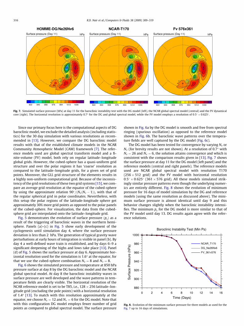
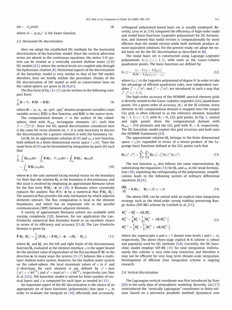
Fig. 7. Simulated surface pressure (hPa) at day 11 for the baroclinic instability test with the DG model (left), the NCAR global spectral model (central) and the FV dynamicalcore (right). The horizontal resolution is approximately 0.7� for the DG and global spectral model, while the FV model employs a resolution of 0:5 � 0:625 .

Fig. 8. Evolution of the minimum surface pressure for three models as used for theFig. 7 up to 16 days of simulations.

316 R.D. Nair et al. / Computers & Fluids 38 (2009) 309–319

Since our primary focus here is the computational aspects of DGbaroclinic model, we exclude the detailed analysis (including statis-tics) for the 30 day simulation with various resolutions as recom-mended in [13]. However, we compare the DG baroclinic modelresults with that of the established climate models in the NCARCommunity Atmospheric Model (CAM) framework [7]. The refer-ence models used are global spectral transform model and a fi-nite-volume (FV) model, both rely on regular latitude–longitudeglobal grids. However, the cubed-sphere has a quasi-uniform gridstructure and over the polar regions it has ‘coarse’ resolution ascompared to the latitude–longitude grids, for a given set of gridpoints. Moreover, the GLL grid structure of the elements results ina highly non-uniform computational grid. Because of the inconsis-tency of the grid resolutions of these two grid systems [15], we com-pare an average grid resolution at the equator of the cubed-sphereby using the approximate relation 90=ðNeðNv � 1ÞÞ, with that ofthe regular spherical grid in polar coordinates. Nevertheless, withthis setup the polar regions of the latitude-longitude sphere getapproximately 30% more grid points as opposed to the polar panelsof the cubed-sphere. For visualization, the data from the cubed-sphere grid are interpolated onto the latitude–longitude grid.

Fig. 5 demonstrates the evolution of surface pressure ðpsÞ as aresult of the triggering of baroclinic waves in the northern hemi-sphere. Panels (a)–(c) in Fig. 5 show early development of thecyclogenesis until simulation day 4, where the surface pressuredeviation is less than 2 hPa. The generation of typical gravity waveperturbations at early hours of integration is visible in panel (b). Byday 4 a well-defined wave train is established, and by days 6–9 asignificant deepening of the highs and lows take place [13]. Panel(d) of Fig. 5 shows the surface pressure at day 6. Approximate hor-izontal resolution used for the simulation is 1.6� at the equator, forthat we use the cubed-sphere combination Ne ¼ 8 and Nv ¼ 8.

Fig. 6 shows the simulated pressure and temperature at 850 hPapressure surface at day 8 by the DG baroclinic model and the NCARglobal spectral model. At day 8 the baroclinic instability waves insurface pressure are well developed and the wave patterns in tem-perature fields are clearly visible. The horizontal resolution of theNCAR reference model is set to be T85, i.e., 128� 256 latitude–lon-gitude grid (excluding the pole points) with a horizontal resolutionof 1.4� [13]. To match with this resolution approximately at theequator, we choose Ne ¼ 12 and Nv ¼ 6 for the DG model. Note thatwith this configuration DG model employs fewer number of gridpoints as compared to global spectral model. The surface pressure

shown in Fig. 6a by the DG model is smooth and free from spectralringing (spurious oscillation) as opposed to the reference modelshown in Fig. 6b. The baroclinic wave patterns over the tempera-ture fields are well captured by the DG model (Fig. 6c).

The DG model has been tested for convergence by varying Ne orNv (for brevity results are not shown). At a resolution of 0.7� withNe ¼ 26 and Nv ¼ 6, the solution attains convergence and which isconsistent with the comparison results given in [13]. Fig. 7 showsthe surface pressure at day 11 for the DG model (left panel) and thereference models (central and right panels). The reference modelsused are NCAR global spectral model with resolution T170(256� 512 grid) and the FV model with horizontal resolution0:5 � 0:625 (361� 576 grid). All these models simulated strik-ingly similar pressure patterns even though the underlying numer-ics are entirely different. Fig. 8 shows the evolution of minimumpressure for 16 days of model simulation by the DG and referencemodels (using the same resolution as discussed above). The mini-mum surface pressure is almost identical until day 9 and thisbehavior changes slightly when the baroclinic instability intensi-fies. The minimum ps for the DG model is more similar to that ofthe FV model until day 13. DG results again agree with the refer-ence solutions.

Table 1Comparison between co-processor and virtual-node modes of IBM Blue Gene/Lsupercomputers

Mode type Coprocessor (CO) Virtual-node (VN)

Clock cycle 0.7 GHz 0.7 GHzMemory/proc 0.5 GB 0.25 GBTasks/node 1 2

R.D. Nair et al. / Computers & Fluids 38 (2009) 309–319 317

4. Parallel implementation

4.1. Domain decomposition

The salient feature of the cubed-sphere geometry is its gridstructure which provides a quasi-uniform grid spacing over thesphere. The cubed-sphere face edges are discontinuous, howeverthey are physically connected by using a set of local transforma-tions provided in [22]. Fig. 9 shows the topological (logical) con-nectivity of the six sub-domains which span the cubed-sphere.Since every sub-domain has the identical square pattern it is rathereasy to tile the entire sphere with rectangular elements as shownin Fig. 1. In other words, for the cubed-sphere the computationaldomain is naturally decomposed into Nelem number of non-overlap-ping rectangular elements.

The parallel implementation of HOMME is based on a hybridMPI/OpenMP approach. HOMME parallel environment is designedto support the element based methods such as spectral elementand discontinuous Galerkin methods. The natural way to paralle-lize the element based method is to allocate a chunk of elementsto each processor. Each element only needs information from adja-cent elements, so the domain decomposition reduces to a standardgraph partitioning problem using algorithm based on either Hilbertspace-filling curve approach by Sagan [26], Dennis et al. [8] or ME-TIS [14].

The approach generates best partitions when Ne ¼ 2‘3m5n,where ‘;m, and n are integers. The first step to partitioning thecomputing grid involves the mapping of the 2-D surface of thecubed-sphere into a linear array. Fig. 10 illustrates the Hilbertspace-filling curve and elements when Nelem ¼ 24. Then the secondstep involves partitioning the linear array into Pg contiguousgroups, where Pg is the number of MPI tasks. The space-fillingcurve partitioning creates contiguous groups of elements andload-balances the computational and communication costs. Formore detail communication frameworks of HOMME, see [8].

z

4 F2 F3F1

F6

F5(Top)

F1

(Bottom)

x

yF

Fig. 9. The logical orientation of the six faces (sub-domains) of the cubed-sphere.

EndStart

Fig. 10. A mapping of a Hilbert space-filling curve for Nelem ¼ 24 cubed-sphere grid.

To perform parallel computing experiments, we employ the2048 processors of a IBM Blue Gene/L (BG/L) supercomputer atNCAR. The configuration of these systems is summarized in Table 1.A Message Passing Interface (MPI) job for IBM BG/L machine can berun in co-processor mode (i.e., a single MPI task runs on each com-pute node) or in virtual-node mode (i.e., two MPI tasks are run oneach compute node). To determine sustained MFLOPS per proces-sor, the number of floating-point operations per time step wasmeasured for the main DG time stepping loop using hardware per-formance counters for IBM supercomputer.

� IBM Blue Gene/L system uses libmpihpm library and its link andcode examples are given as follows:

add -L$(BGL_LIBRARY_PATH) -lmpihpm_f -

lbgl_perfctr.rts. . .

call trace_start()call dg3d_advance()call trace_stop(). . .

4.2. Parallel performance

To assess parallel performance we consider baroclinic instabil-ity test [13]. Note that all writing and printing functions are turnedoff during performance evaluations. Table 2 summarizes thedynamical core configurations for 3-D model used in parallel per-formance experiments (note that the R–K time steps used are notoptimal).

Fig. 11 demonstrates parallel performance, where 2048 proces-sors of a IBM Blue Gene/L machine sustains between 248 and 257MFLOPS per processor with coprocessor mode and sustains be-tween 220 and 247 MFLOPS per processor with virtual-node modefor 1� horizontal resolution (i.e., Nelem ¼ 1944). For 0.5� horizontalresolution (i.e., Nelem ¼ 7776), 2048 processors of a IBM Blue Gene/L machine sustains between 249 and 261 MFLOPS per processorwith coprocessor mode and sustains between 232 and 248 MFLOPSper processor with virtual-node mode. The CPU cost in wall clockhours is shown in Fig. 12.

Table 3 summaries the percentage of peak performance forstrong scaling results for 2048 processors of a IBM Blue Gene/L sys-tem. Two thousand and fourty-eight processors of a IBM BlueGene/L machine sustains 9.5% and 9.3% of peak performance forcoprocessor and virtual-node modes, respectively.

Table 2Summary of dynamical core configurations for Baroclinic Instability Test used in 3-DDGM model on HOMME

Horizontalresolution

Vertical resolutionðNlevÞ

Number of elementsðNelemÞ

Time stepðDtÞ

1� 26 1944 6 s0.5� 26 7776 3 s

32 64 128 256 512 1024 20480

50

100

150

200

250

300

Processor

MF

LOP

Sustained FLOP/Processor

1944 elements: 1 task/node (CO)1944 elements: 2 task/node (VN)7776 elements: 1 tasks/node (CO)7776 elements: 2 tasks/node (VN)

Fig. 11. Parallel performance (i.e., strong scaling) results on 2048 processors of aIBM BG/L supercomputer at NCAR.

32 64 128 256 512 1024 2048

10−1

100

101

Processor

CP

U H

our

1 Day Simulation CPU Cost Per Hour

1944 elements: 1 task/node (CO)1944 elements: 2 task/node (VN)7776 elements: 1 tasks/node (CO)7776 elements: 2 tasks/node (VN)

Fig. 12. The CPU cost in wall clock hour as a function of processors on 2048 pro-cessors of a IBM BG/L supercomputer at NCAR.

Table 3Summary of strong scaling results for 2048 processors of a IBM BG/L supercomputerat NCAR

Resource Sustained MFLOPS % of peak performance

1944 elements: 1 task/node (CO) 257 9.21944 elements: 2 tasks/node (VN) 247 8.87776 elements: 1 task/node (CO) 261 9.37776 elements: 2 tasks/node (VN) 248 8.9

318 R.D. Nair et al. / Computers & Fluids 38 (2009) 309–319

5. Conclusion

A conservative high-order discontinuous Galerkin (DG) baro-clinic model has been developed and implemented in NCAR’shigh-order method modeling environment (HOMME). The 3-DDG model rely on hydrostatic primitive equations cast in flux-from.The computational domain is the singularity-free cubed-spheregeometry. The DG discretization uses high-order nodal basis set

of Lagrange–Legendre polynomials and fluxes of inter-elementboundaries are approximated with Lax–Friedrichs numerical flux.The vertical discretization follows the 1-D vertical terrain-follow-ing Lagrangian coordinates approach. Consequently, the 3-D atmo-sphere is divided into a finite number of Lagrangian 2-D horizontalsurfaces (layers) and DG discretization is performed for each layer.Over time, the Lagrangian surfaces are subject to deformation, andtherefore the state variables are periodically remapped onto a ref-erence coordinate. The vertical remapping is performed with theconservative cell-integrated semi-Lagrangian method.

The time integration of the model rely on the explicit third-or-der strong-stability preserving Runge–Kutta scheme. The DGdynamical core is validated using a baroclinic instability test andresults are compared with that of the NCAR global spectral modeland a finite-volume model available in community atmosphericmodeling framework. The DG model successfully simulated baro-clinic instability growth and the results are comparable with thatof the reference models. Idealized tests show that the new modelsimulation is accurate, smooth and free from ‘spectral ringing’(spurious oscillations) as opposed to the global spectral model.

However, the DG baroclinic model employs explicit Runge–Kut-ta time integration with moderate time step size resulting in a low-er integration rate. This may not be adequate for long-term climatesimulations. New time integration schemes for the baroclinic mod-el is under investigation. This includes semi-implicit, implicit–ex-plicit Runge–Kutta and the Rosenbrock class of time integrators.The vertical Lagrangian treatment is an elegant approach by whichthe 3D model can be treated as vertically-stacked shallow water(2D) models. Nevertheless, the remapping frequency used for thepresent study is somewhat ad hoc, and more rigorous studies arerequired in this regard.

Parallel experiments are tested on 2048 processors of a IBMBlue Gene/L supercomputer at NCAR. Conservative 3-D DG baro-clinic model sustains 9.3% peak performance (i.e., 261 MFLOPS/processor) for IBM Blue Gene/L’s coprocessor mode and sustains8.9% peak performance (i.e., 248 MFLOPS/processor) for IBM BlueGene/L’s virtual-node mode. The preliminary performance studywith DG model is encouraging and comparable to that of the SEbaroclinic model in HOMME. Extending the new DG model to afully-fledged climate model with realistic physics packages andscaling up to Oð100 KÞ processors is our ultimate goal.

Acknowledgements

The Authors would like to thank Prof. Christiane Jablonowskifor the baroclinic instability test comparison data, Dr. John Dennisfor the performance study support and Dr. Peter Lauritzen for theinternal review of the manuscript. This project is supported bythe NSF sponsorship of the NCAR and DOE awards #DE-FG02-04ER63870 and #DE-FG02-07ER64464. Computer time is providedthrough the NSF MRI Grants CNS-0421498, CNS-0420873, andCNS-0420985, and through the IBM Shared University ResearchProgram.

References

[1] Arakawa A, Suarez MJ. Vertical differencing of the primitive equations in sigmacoordinates. Mon Weather Rev 1983;111:34–45.

[2] Bhanot G, Dennis JM, Edwards J, Grabowski W, Gupta M, Jordan K, et al. Earlyexperiences with the 360T IBM BlueGene/L Platform. Int J Comput Meth2008;5, in press.

[3] Choi H-W, Nair RD, Tufo HM. A scalable high-order discontinuous Galerkinmethods for global atmospheric modeling. In: Proceedings of the internationalconference on parallel computational fluid dynamics. Busan, SouthKorea: Elsevier; 2006.

[4] Cockburn B. An introduction to the discontinuous-Galerkin method forconvection-dominated problems. In: Quarteroni A, editor. Lecture notes inmathematics: advanced numerical approximation of nonlinear hyperbolicequations, vol. 1697. Springer; 1997. p. 151–268.

R.D. Nair et al. / Computers & Fluids 38 (2009) 309–319 319

[5] Cockburn B, Hou S, Shu C-W. TVB Runge–Kutta local projection discontinuousGalerkin finite element method for conservation laws IV: themultidimensional case. Math Comp 1990;54:545–81.

[6] Cockburn B, Karniadakis GE, Shu C-W. Discontinuous Gakerkin methods:theory, computation, and applications. Lecture notes in computational scienceand engineering, vol. 11. Springer; 2000. p. 1–470.

[7] Collins WD, Rasch PJ, Boville BA, Hack JJ, McCaa JR, Williamson DL, et al. Theformulation and atmospheric simulation of the community atmosphericmodel version 3 (CAM3). J Clim 2006;19:2144–61.

[8] Dennis JM, Levy M, Nair RD, Tufo HM, Voran T. Towards an efficient andscalable discontinuous Galerkin atmospheric model. Proceedings of the 19thIEEE International Parallel and Distributed Processing Symposium, 4–8 April2005, 7 pp.

[9] HOMME: high-order methods modeling environment. National Center forAtmospheric Research (NCAR); 2006. <http://www.homme.ucar.edu>.

[10] Fournier A, Taylor MA, Tribbia JJ. A spectral element atmospheric model(seam): high-resolution parallel computation and local resolution of regionaldynamics. Mon Weather Rev 2004;132:726–48.

[11] Gottlieb S, Shu C-W, Tadmor E. Strong stability-preserving high-order timediscretization methods. SIAM Rev. 2001;43(1):89–112.

[12] Held IM, Suarez MJ. A proposal for the intercomparison of the dynamical coresof atmospheric general circulation models. Bull Amer Meteor Soc1994;75(10):1825–30.

[13] Jablonowski C, Williamson DL. A Baroclinic instability test case foratmospheric model dynamical cores. Quart J Royal Meteorol Soc2006;132:2943–75.

[14] Karypis G, Kumar V. METIS Family of multilevel partitioning algorithms.University of Minnesota, Department of Computer Science; 1998. <http://glaros.dtc.umn.edu/gkhome/views/metis>.

[15] Lauritzen PH, Nair RD. Monotone and conservative cascade remappingbetween spherical grids (CaRS): regular latitude–longitude and cubed-spheregrids. Mon Weather Rev 2008;136:1416–32.

[16] Levy MN, Nair RD, Tufo HM. High-order Galerkin methods for scalable globalatmospheric models. Comput Geosci 2007;33:1022–35.

[17] Lin S-J. A ‘‘vertically-Lagrangian” finite-volume dynamical core for globalmodels. Mon Weather Rev 2004;132:2293–307.

[18] Loft RD, Thomas SJ, Dennis JM. Terascale spectral element dynamical core foratmospheric general circulation models. Supercomputing 2001. In: ACM/IEEEconference, Denver; 2001.

[19] Machenhauer B, Kass E, Lauritzen PH. Handbook of numerical analysis: specialvolume on computational methods for the atmosphere and the oceans.Elsevier 2008; in press.

[20] Nair RD, Manchenhauer B. The mass-conservative cell-integrated semi-Lagrangian advection scheme on the sphere. Mon Weather Rev2002;130:649–67.

[21] Nair RD, Thomas SJ, Loft RD. A Discontinuous Galerkin global shallow watermodel. Mon Weather Rev 2005;133:876–88.

[22] Nair RD, Thomas SJ, Loft RD. A Discontinuous Galerkin transport scheme on thecubed sphere. Mon Weather Rev 2005;133:814–28.

[23] Nair RD, Tufo HM. Petascale atmospheric general circulation models. J Phys:Conf Ser 2007;78. doi:10.1088/1742–6596/78/1/012078.

[24] Ringler TD, Heikes RP, Randall DA. Modeling the atmospheric generalcirculation using a spherical geodesic grid: a new class of dynamical cores.Mon Weather Rev 2000;128:2471–89.

[25] Sadourny R. Conservative finite-difference approximations of the primitiveequations on quasi-uniform spherical grids. Mon Weather Rev1972;100:136–44.

[26] Sagan H. Space-filling curves. Springer-Verlag; 1994.[27] Simmons AJ, Burridge DM. An energy and angular-momentum conserving

vertical finite-difference scheme and hybrid vertical coordinates. MonWeather Rev 1981;109:758–66.

[28] St-Cyr A, Jablonowski C, Dennis JM, Tufo HM, Thomas SJ. A comparison of twoshallow water models with non-conforming adaptive grids. Mon. Wea. Rev.2008;136: In Press.

[29] Starr VP. A quasi-Lagrangian system of hydrodynamical equations. J Meterol1945;2(1):227–37.

[30] Taylor MA, Tribbia JJ, Iskandrani M. The spectral element method for theshallow water equations on the sphere. J Comput Phys 1997;130:92–108.

[31] Thomas SJ, Loft RD. Semi-implicit spectral element atmospheric model. J SciComput 2002;17:339–50.

[32] Toro EF. Riemann solvers and numerical methods for fluid dynamics. Springer;1999.

[33] Washington WM, Parkinson CL. An introduction to three-dimensional climatemodeling. University Science Books; 2005.

[34] Zhang H, Rancic M. A global eta model on quasi-uniform grids. Quart J RoyMeteo Soc 2007;133:517–28.