Computer Vision Lecture 5 ng‘19 · 7 ng‘19 Mixture of Gaussians • One generative model is a...

1

Pe

rce

ptu

al

an

d S

en

so

ry A

ug

me

nte

d C

om

pu

tin

gC

om

pu

ter

Vis

ion

Su

mm

er‘

19

Computer Vision – Lecture 5

Segmentation

30.04.2019

Bastian Leibe

Visual Computing Institute

RWTH Aachen University

http://www.vision.rwth-aachen.de/

[email protected] Pe

rce

ptu

al

an

d S

en

so

ry A

ug

me

nte

d C

om

pu

tin

gC

om

pu

ter

Vis

ion

Su

mm

er‘

19

Course Outline

• Image Processing Basics

Recap: Structure Extraction

• Segmentation

Segmentation as Clustering

Graph-theoretic Segmentation

• Recognition

Global Representations

Subspace representations

• Local Features & Matching

• Object Categorization

• 3D Reconstruction

2

Pe

rce

ptu

al

an

d S

en

so

ry A

ug

me

nte

d C

om

pu

tin

gC

om

pu

ter

Vis

ion

Su

mm

er‘

19

Recap: Hough Transform

• How can we use this to find the most likely parameters

(𝑚, 𝑏) for the most prominent line in the image space?

Let each edge point in image space vote for a set of possible

parameters in Hough space

Accumulate votes in discrete set of bins; parameters with the most

votes indicate line in image space.

3

x

y

m

b

Image space Hough (parameter) space

Slide credit: Steve Seitz

b = –x1m + y1

(x0, y0)

(x1, y1)

𝑚1

𝑏1

𝑦 = 𝑚1𝑥 + 𝑏1

Pe

rce

ptu

al

an

d S

en

so

ry A

ug

me

nte

d C

om

pu

tin

gC

om

pu

ter

Vis

ion

Su

mm

er‘

19

Recap: Hough Transf. Polar Parametrization

• Usual 𝑚, 𝑏 parameter space problematic:

Can take on infinite values, undefined for vertical lines.

• Point in image space

Sinusoid segment in

Hough space

4

[0,0]

d

x

y

: perpendicular distance from

line to origin

: angle the perpendicular

makes with the x-axis

d

Slide adapted from Steve Seitz

𝑥 cos 𝜃 + 𝑦 sin 𝜃 = 𝑑

Pe

rce

ptu

al

an

d S

en

so

ry A

ug

me

nte

d C

om

pu

tin

gC

om

pu

ter

Vis

ion

Su

mm

er‘

19

Recap: Hough Transform for Circles

• Circle: center (𝑎, 𝑏) and radius 𝑟

• For an unknown radius 𝑟, unknown gradient direction

5B. Leibe

Hough spaceImage space

b

r

a

222 )()( rbyax ii

Slide credit: Kristen Grauman

Pe

rce

ptu

al

an

d S

en

so

ry A

ug

me

nte

d C

om

pu

tin

gC

om

pu

ter

Vis

ion

Su

mm

er‘

19

Recap: Generalized Hough Transform

• What if we want to detect arbitrary shapes defined by

boundary points and a reference point?

6B. Leibe

Image space

x a

p1

θ

p2

θ

At each boundary point,

compute displacement vector:

𝑟 = 𝑎 – 𝑝𝑖.

For a given model shape:

store these vectors in a table

indexed by gradient

orientation 𝜃.

[Dana H. Ballard, Generalizing the Hough Transform to Detect Arbitrary Shapes, 1980]


2

Pe

rce

ptu

al

an

d S

en

so

ry A

ug

me

nte

d C

om

pu

tin

gC

om

pu

ter

Vis

ion

Su

mm

er‘

19

Recap: Generalized Hough Transform

To detect the model shape in a new image:

• For each edge point

Index into table with its gradient orientation 𝜃

Use retrieved 𝑟 vectors to vote for position of reference point

• Peak in this Hough space is reference point with most

supporting edges

7Slide credit: Kristen Grauman

Voting locations

for test points

Displacement vectors

based on model shape Pe

rce

ptu

al

an

d S

en

so

ry A

ug

me

nte

d C

om

pu

tin

gC

om

pu

ter

Vis

ion

Su

mm

er‘

19

Topics of This Lecture

• Segmentation and grouping

Gestalt principles

Image Segmentation

• Segmentation as clustering

k-Means

Feature spaces

• Probabilistic clustering

Mixture of Gaussians, EM

• Model-free clustering

Mean-Shift clustering

8B. Leibe

Pe

rce

ptu

al

an

d S

en

so

ry A

ug

me

nte

d C

om

pu

tin

gC

om

pu

ter

Vis

ion

Su

mm

er‘

19

Examples of Grouping in Vision

9B. Leibe

Determining image regions

Grouping video frames into shots

Object-level grouping

Figure-ground


What things should

be grouped?

What cues

indicate groups?

Pe

rce

ptu

al

an

d S

en

so

ry A

ug

me

nte

d C

om

pu

tin

gC

om

pu

ter

Vis

ion

Su

mm

er‘

19

The Gestalt School

• Grouping is key to visual perception

• Elements in a collection can have properties that result

from relationships

“The whole is greater than the sum of its parts”

10

Illusory/subjective

contoursOcclusion

Familiar configuration

http://en.wikipedia.org/wiki/Gestalt_psychology

Slide credit: Svetlana Lazebnik Image source: Steve Lehar

Pe

rce

ptu

al

an

d S

en

so

ry A

ug

me

nte

d C

om

pu

tin

gC

om

pu

ter

Vis

ion

Su

mm

er‘

19

Gestalt Theory

• Gestalt: whole or group

Whole is greater than sum of its parts

Relationships among parts can yield new properties/features

• Psychologists identified series of factors that predispose set

of elements to be grouped (by human visual system)

11B. Leibe

Untersuchungen zur Lehre von der Gestalt,

Psychologische Forschung, Vol. 4, pp. 301-350, 1923

http://psy.ed.asu.edu/~classics/Wertheimer/Forms/forms.htm

“I stand at the window and see a house, trees, sky.

Theoretically I might say there were 327 brightnesses

and nuances of colour. Do I have "327"? No. I have sky,

house, and trees.”

Max Wertheimer(1880-1943)

Pe

rce

ptu

al

an

d S

en

so

ry A

ug

me

nte

d C

om

pu

tin

gC

om

pu

ter

Vis

ion

Su

mm

er‘

19

Gestalt Factors

• These factors make intuitive sense, but are very difficult to translate

into algorithms.12

B. Leibe Image source: Forsyth & Ponce

http://en.wikipedia.org/wiki/Gestalt_psychology

http://psy.ed.asu.edu/~classics/Wertheimer/Forms/forms.htm

3

Pe

rce

ptu

al

an

d S

en

so

ry A

ug

me

nte

d C

om

pu

tin

gC

om

pu

ter

Vis

ion

Su

mm

er‘

19

Continuity through Occlusion Cues

13B. Leibe

Pe

rce

ptu

al

an

d S

en

so

ry A

ug

me

nte

d C

om

pu

tin

gC

om

pu

ter

Vis

ion

Su

mm

er‘

19


14B. Leibe

Continuity, explanation by occlusion

Pe

rce

ptu

al

an

d S

en

so

ry A

ug

me

nte

d C

om

pu

tin

gC

om

pu

ter

Vis

ion

Su

mm

er‘

19


15B. Leibe Image source: Forsyth & Ponce

Pe

rce

ptu

al

an

d S

en

so

ry A

ug

me

nte

d C

om

pu

tin

gC

om

pu

ter

Vis

ion

Su

mm

er‘

19


16B. Leibe Image source: Forsyth & Ponce

Pe

rce

ptu

al

an

d S

en

so

ry A

ug

me

nte

d C

om

pu

tin

gC

om

pu

ter

Vis

ion

Su

mm

er‘

19

The Ultimate Gestalt?

17B. Leibe

Pe

rce

ptu

al

an

d S

en

so

ry A

ug

me

nte

d C

om

pu

tin

gC

om

pu

ter

Vis

ion

Su

mm

er‘

19

Image Segmentation

• Goal: identify groups of pixels that go together

18B. LeibeSlide credit: Steve Seitz, Kristen Grauman

4

Pe

rce

ptu

al

an

d S

en

so

ry A

ug

me

nte

d C

om

pu

tin

gC

om

pu

ter

Vis

ion

Su

mm

er‘

19

The Goals of Segmentation

• Separate image into coherent “objects”

19B. Leibe

Image Human segmentation

Slide credit: Svetlana Lazebnik

Pe

rce

ptu

al

an

d S

en

so

ry A

ug

me

nte

d C

om

pu

tin

gC

om

pu

ter

Vis

ion

Su

mm

er‘

19



Gestalt principles

Image Segmentation


k-Means

Feature spaces





20B. Leibe

Pe

rce

ptu

al

an

d S

en

so

ry A

ug

me

nte

d C

om

pu

tin

gC

om

pu

ter

Vis

ion

Su

mm

er‘

19

Image Segmentation: Toy Example

• These intensities define the three groups.

• We could label every pixel in the image according to which

of these primary intensities it is.

i.e., segment the image based on the intensity feature.

• What if the image isn’t quite so simple?

21B. Leibe

intensity

input image

black pixelsgray

pixels

white

pixels

1 23


Pe

rce

ptu

al

an

d S

en

so

ry A

ug

me

nte

d C

om

pu

tin

gC

om

pu

ter

Vis

ion

Su

mm

er‘

19

22B. Leibe

Pix

el co

un

t

Input image

Input imageIntensity

Pix

el co

un

t

Intensity


Pe

rce

ptu

al

an

d S

en

so

ry A

ug

me

nte

d C

om

pu

tin

gC

om

pu

ter

Vis

ion

Su

mm

er‘

19 • Now how to determine the three main intensities that define

our groups?

• We need to cluster.

23B. Leibe

Input imageIntensity

Pix

el

co

un

t


Pe

rce

ptu

al

an

d S

en

so

ry A

ug

me

nte

d C

om

pu

tin

gC

om

pu

ter

Vis

ion

Su

mm

er‘

19

• Goal: choose three “centers” as the representative

intensities, and label every pixel according to which of these

centers it is nearest to.

• Best cluster centers are those that minimize SSD between

all points and their nearest cluster center ci:

24B. LeibeSlide credit: Kristen Grauman

0 190 255

1 23

Intensity

5

Pe

rce

ptu

al

an

d S

en

so

ry A

ug

me

nte

d C

om

pu

tin

gC

om

pu

ter

Vis

ion

Su

mm

er‘

19

Clustering

• With this objective, it is a “chicken and egg” problem:

If we knew the cluster centers, we could allocate points to groups by

assigning each to its closest center.

If we knew the group memberships, we could get the centers by

computing the mean per group.


Pe

rce

ptu

al

an

d S

en

so

ry A

ug

me

nte

d C

om

pu

tin

gC

om

pu

ter

Vis

ion

Su

mm

er‘

19

K-Means Clustering

• Basic idea: randomly initialize the k cluster centers, and

iterate between the two steps we just saw.

1. Randomly initialize the cluster centers, c1, ..., cK

2. Given cluster centers, determine points in each cluster

– For each point p, find the closest ci. Put p into cluster i

3. Given points in each cluster, solve for ci

– Set ci to be the mean of points in cluster i

4. If ci have changed, repeat Step 2

• Properties Will always converge to some solution

Can be a “local minimum”

– Does not always find the global minimum of objective function:

26B. LeibeSlide credit: Steve Seitz

Pe

rce

ptu

al

an

d S

en

so

ry A

ug

me

nte

d C

om

pu

tin

gC

om

pu

ter

Vis

ion

Su

mm

er‘

19


27B. Leibe

K=2

K=3

img_as_col = double(im(:));

cluster_membs = kmeans(img_as_col, K);

labelim = zeros(size(im));

for i=1:k

inds = find(cluster_membs==i);

meanval = mean(img_as_column(inds));

labelim(inds) = meanval;

end


Pe

rce

ptu

al

an

d S

en

so

ry A

ug

me

nte

d C

om

pu

tin

gC

om

pu

ter

Vis

ion

Su

mm

er‘

19

K-Means++

• Can we prevent arbitrarily bad local minima?

1. Randomly choose first center.

2. Pick new center with prob. proportional to

(Contribution of p to total error)

3. Repeat until k centers.

• Expected error = O(log k) * optimal

28B. Leibe

Arthur & Vassilvitskii 2007

Slide credit: Steve Seitz

Pe

rce

ptu

al

an

d S

en

so

ry A

ug

me

nte

d C

om

pu

tin

gC

om

pu

ter

Vis

ion

Su

mm

er‘

19

Feature Space

• Depending on what we choose as the feature space,

we can group pixels in different ways.

• Grouping pixels based on

intensity similarity

• Feature space: intensity value (1D)


Pe

rce

ptu

al

an

d S

en

so

ry A

ug

me

nte

d C

om

pu

tin

gC

om

pu

ter

Vis

ion

Su

mm

er‘

19

Feature Space



• Grouping pixels based

on color similarity

• Feature space: color value (3D) 30

B. Leibe

R=255

G=200

B=250

R=245

G=220

B=248

R=15

G=189

B=2

R=3

G=12

B=2R

G

B


http://theory.stanford.edu/~sergei/slides/BATS-Means.pdf

6

Pe

rce

ptu

al

an

d S

en

so

ry A

ug

me

nte

d C

om

pu

tin

gC

om

pu

ter

Vis

ion

Su

mm

er‘

19




• Grouping pixels based

on texture similarity

• Feature space: filter bank responses (e.g., 24D) 31

B. Leibe

Filter bank of

24 filters

F24

F2

F1

…


Pe

rce

ptu

al

an

d S

en

so

ry A

ug

me

nte

d C

om

pu

tin

gC

om

pu

ter

Vis

ion

Su

mm

er‘

19

Smoothing Out Cluster Assignments

• Assigning a cluster label per pixel may yield outliers:

• How can we ensure they

are spatially smooth?

32B. Leibe

1 2

3

?

Original Labeled by cluster center’s

intensity


Pe

rce

ptu

al

an

d S

en

so

ry A

ug

me

nte

d C

om

pu

tin

gC

om

pu

ter

Vis

ion

Su

mm

er‘

19




• Grouping pixels based on

intensity+position similarity

Simple way to encode both similarity and proximity.

What could be a problem with this solution?33

B. LeibeSlide credit: Kristen Grauman

X

Intensity

Y

Pe

rce

ptu

al

an

d S

en

so

ry A

ug

me

nte

d C

om

pu

tin

gC

om

pu

ter

Vis

ion

Su

mm

er‘

19

Summary K-Means

• Pros

Simple, fast to compute

Converges to local minimum

of within-cluster squared error

• Cons/issues

Setting k?

Sensitive to initial centers

Sensitive to outliers

Detects spherical clusters only

Assuming means can be

computed


Pe

rce

ptu

al

an

d S

en

so

ry A

ug

me

nte

d C

om

pu

tin

gC

om

pu

ter

Vis

ion

Su

mm

er‘

19



Gestalt principles

Image Segmentation


k-Means

Feature spaces





37B. Leibe

Pe

rce

ptu

al

an

d S

en

so

ry A

ug

me

nte

d C

om

pu

tin

gC

om

pu

ter

Vis

ion

Su

mm

er‘

19

Probabilistic Clustering

• Basic questions

What’s the probability that a point x is in cluster m?

What’s the shape of each cluster?

• K-means doesn’t answer these questions.

• Basic idea

Instead of treating the data as a bunch of points, assume that they

are all generated by sampling a continuous function.

This function is called a generative model.

Defined by a vector of parameters θ


7

Pe

rce

ptu

al

an

d S

en

so

ry A

ug

me

nte

d C

om

pu

tin

gC

om

pu

ter

Vis

ion

Su

mm

er‘

19

Mixture of Gaussians

• One generative model is a mixture of Gaussians (MoG)

K Gaussian blobs with means ¹j, cov. matrices §j, dim. D

Blob j is selected with probability ¼j

The likelihood of observing x is a weighted mixture of Gaussians

39B. LeibeSlide adapted from Steve Seitz

p(xjµj) =1

(2¼)D=2j§jj1=2exp

½¡1

2(x¡¹j)T§¡1j (x¡¹j)

¾

µ = (¼1;¹1;§1; : : : ; ¼M;¹M;§M)

Pe

rce

ptu

al

an

d S

en

so

ry A

ug

me

nte

d C

om

pu

tin

gC

om

pu

ter

Vis

ion

Su

mm

er‘

19

Expectation Maximization (EM)

• Goal

Find blob parameters µ that maximize the likelihood function:

• Approach:1. E-step: given current guess of blobs, compute ownership of each point

2. M-step: given ownership probabilities, update blobs to maximize

likelihood function

3. Repeat until convergence40

B. LeibeSlide credit: Steve Seitz

Pe

rce

ptu

al

an

d S

en

so

ry A

ug

me

nte

d C

om

pu

tin

gC

om

pu

ter

Vis

ion

Su

mm

er‘

19

EM Algorithm

• Expectation-Maximization (EM) Algorithm

E-Step: softly assign samples to mixture components

M-Step: re-estimate the parameters (separately for each mixture

component) based on the soft assignments

41B. Leibe

8j = 1; : : : ;K; n= 1; : : : ;N

¼̂newj Ã N̂j

N

¹̂newj Ã 1

N̂j

NX

n=1

°j(xn)xn

§̂newj Ã 1

N̂j

NX

n=1

°j(xn)(xn ¡ ¹̂newj )(xn ¡ ¹̂newj )T

N̂j ÃNX

n=1

°j(xn) = soft number of samples labeled j

Slide adapted from Bernt Schiele

Pe

rce

ptu

al

an

d S

en

so

ry A

ug

me

nte

d C

om

pu

tin

gC

om

pu

ter

Vis

ion

Su

mm

er‘

19

Applications of EM

• Turns out this is useful for all sorts of problems

Any clustering problem

Any model estimation problem

Missing data problems

Finding outliers

Segmentation problems

– Segmentation based on color

– Segmentation based on motion

– Foreground/background separation

...


Pe

rce

ptu

al

an

d S

en

so

ry A

ug

me

nte

d C

om

pu

tin

gC

om

pu

ter

Vis

ion

Su

mm

er‘

19

Segmentation with EM

43B. Leibe Image source: Serge Belongie

k=2 k=3 k=4 k=5

EM segmentation results

Original image

Pe

rce

ptu

al

an

d S

en

so

ry A

ug

me

nte

d C

om

pu

tin

gC

om

pu

ter

Vis

ion

Su

mm

er‘

19

Summary: Mixtures of Gaussians, EM

• Pros

Probabilistic interpretation

Soft assignments between data points and clusters

Generative model, can predict novel data points

Relatively compact storage

• Cons

Local minima

– k-means is NP-hard even with k=2

Initialization

– Often a good idea to start with some k-means iterations.

Need to know number of components

– Solutions: model selection (AIC, BIC), Dirichlet process mixture

Need to choose generative model

Numerical problems are often a nuisance44

B. Leibe

8

Pe

rce

ptu

al

an

d S

en

so

ry A

ug

me

nte

d C

om

pu

tin

gC

om

pu

ter

Vis

ion

Su

mm

er‘

19



Gestalt principles

Image segmentation


k-Means

Feature spaces





45B. Leibe

Pe

rce

ptu

al

an

d S

en

so

ry A

ug

me

nte

d C

om

pu

tin

gC

om

pu

ter

Vis

ion

Su

mm

er‘

19

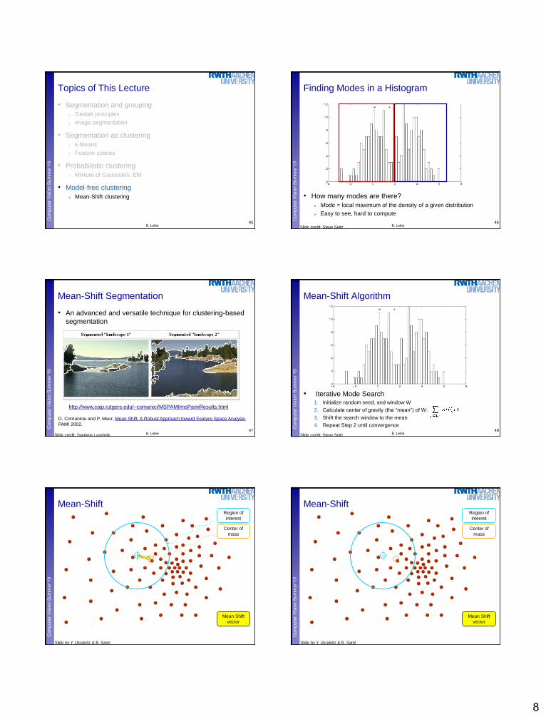
Finding Modes in a Histogram

• How many modes are there?

Mode = local maximum of the density of a given distribution

Easy to see, hard to compute


Pe

rce

ptu

al

an

d S

en

so

ry A

ug

me

nte

d C

om

pu

tin

gC

om

pu

ter

Vis

ion

Su

mm

er‘

19

Mean-Shift Segmentation

• An advanced and versatile technique for clustering-based

segmentation

47B. Leibe

http://www.caip.rutgers.edu/~comanici/MSPAMI/msPamiResults.html

D. Comaniciu and P. Meer, Mean Shift: A Robust Approach toward Feature Space Analysis,

PAMI 2002.


Pe

rce

ptu

al

an

d S

en

so

ry A

ug

me

nte

d C

om

pu

tin

gC

om

pu

ter

Vis

ion

Su

mm

er‘

19

Mean-Shift Algorithm

• Iterative Mode Search1. Initialize random seed, and window W

2. Calculate center of gravity (the “mean”) of W:

3. Shift the search window to the mean

4. Repeat Step 2 until convergence48

B. LeibeSlide credit: Steve Seitz

Pe

rce

ptu

al

an

d S

en

so

ry A

ug

me

nte

d C

om

pu

tin

gC

om

pu

ter

Vis

ion

Su

mm

er‘

19

Region of

interest

Center of

mass

Mean Shift

vector

Mean-Shift

Slide by Y. Ukrainitz & B. Sarel

Pe

rce

ptu

al

an

d S

en

so

ry A

ug

me

nte

d C

om

pu

tin

gC

om

pu

ter

Vis

ion

Su

mm

er‘

19

Region of

interest

Center of

mass

Mean Shift

vector

Mean-Shift



http://www.caip.rutgers.edu/~comanici/Papers/MsRobustApproach.pdf

9

Pe

rce

ptu

al

an

d S

en

so

ry A

ug

me

nte

d C

om

pu

tin

gC

om

pu

ter

Vis

ion

Su

mm

er‘

19

Region of

interest

Center of

mass

Mean Shift

vector

Mean-Shift


Pe

rce

ptu

al

an

d S

en

so

ry A

ug

me

nte

d C

om

pu

tin

gC

om

pu

ter

Vis

ion

Su

mm

er‘

19

Region of

interest

Center of

mass

Mean Shift

vector

Mean-Shift


Pe

rce

ptu

al

an

d S

en

so

ry A

ug

me

nte

d C

om

pu

tin

gC

om

pu

ter

Vis

ion

Su

mm

er‘

19

Region of

interest

Center of

mass

Mean Shift

vector

Mean-Shift


Pe

rce

ptu

al

an

d S

en

so

ry A

ug

me

nte

d C

om

pu

tin

gC

om

pu

ter

Vis

ion

Su

mm

er‘

19

Region of

interest

Center of

mass

Mean Shift

vector

Mean-Shift


Pe

rce

ptu

al

an

d S

en

so

ry A

ug

me

nte

d C

om

pu

tin

gC

om

pu

ter

Vis

ion

Su

mm

er‘

19

Region of

interest

Center of

mass

Mean-Shift


Pe

rce

ptu

al

an

d S

en

so

ry A

ug

me

nte

d C

om

pu

tin

gC

om

pu

ter

Vis

ion

Su

mm

er‘

19

Tessellate the space

with windows

Run the procedure in parallel


Real Modality Analysis

10

Pe

rce

ptu

al

an

d S

en

so

ry A

ug

me

nte

d C

om

pu

tin

gC

om

pu

ter

Vis

ion

Su

mm

er‘

19

The blue data points were traversed by the windows towards the mode.


Real Modality Analysis

Pe

rce

ptu

al

an

d S

en

so

ry A

ug

me

nte

d C

om

pu

tin

gC

om

pu

ter

Vis

ion

Su

mm

er‘

19

Mean-Shift Clustering

• Cluster: all data points in the attraction basin of a mode

• Attraction basin: the region for which all trajectories lead to

the same mode

58B. LeibeSlide by Y. Ukrainitz & B. Sarel

Pe

rce

ptu

al

an

d S

en

so

ry A

ug

me

nte

d C

om

pu

tin

gC

om

pu

ter

Vis

ion

Su

mm

er‘

19

Mean-Shift Clustering/Segmentation

• Find features (color, gradients, texture, etc)

• Initialize windows at individual pixel locations

• Perform mean shift for each window until convergence

• Merge windows that end up near the same “peak” or mode

59B. LeibeSlide credit: Svetlana Lazebnik

Pe

rce

ptu

al

an

d S

en

so

ry A

ug

me

nte

d C

om

pu

tin

gC

om

pu

ter

Vis

ion

Su

mm

er‘

19

Mean-Shift Segmentation Results

60B. Leibe



Pe

rce

ptu

al

an

d S

en

so

ry A

ug

me

nte

d C

om

pu

tin

gC

om

pu

ter

Vis

ion

Su

mm

er‘

19

More Results


Pe

rce

ptu

al

an

d S

en

so

ry A

ug

me

nte

d C

om

pu

tin

gC

om

pu

ter

Vis

ion

Su

mm

er‘

19

More Results



11

Pe

rce

ptu

al

an

d S

en

so

ry A

ug

me

nte

d C

om

pu

tin

gC

om

pu

ter

Vis

ion

Su

mm

er‘

19

Problem: Computational Complexity

• Need to shift many windows…

• Many computations will be redundant.B. Leibe

Pe

rce

ptu

al

an

d S

en

so

ry A

ug

me

nte

d C

om

pu

tin

gC

om

pu

ter

Vis

ion

Su

mm

er‘

19

Speedups: Basin of Attraction

1. Assign all points within radius r of end point to the mode.

B. Leibe

r

Pe

rce

ptu

al

an

d S

en

so

ry A

ug

me

nte

d C

om

pu

tin

gC

om

pu

ter

Vis

ion

Su

mm

er‘

19

Speedups

2. Assign all points within radius r/c of the search path to the mode.

B. Leibe

r=c

Pe

rce

ptu

al

an

d S

en

so

ry A

ug

me

nte

d C

om

pu

tin

gC

om

pu

ter

Vis

ion

Su

mm

er‘

19

Summary Mean-Shift

• Pros

General, application-independent tool

Model-free, does not assume any prior shape (spherical, elliptical,

etc.) on data clusters

Just a single parameter (window size h)

– h has a physical meaning (unlike k-means)

Finds variable number of modes

Robust to outliers

• Cons

Output depends on window size

Window size (bandwidth) selection is not trivial

Computationally (relatively) expensive

Does not scale well with dimension of feature space


Pe

rce

ptu

al

an

d S

en

so

ry A

ug

me

nte

d C

om

pu

tin

gC

om

pu

ter

Vis

ion

Su

mm

er‘

19

Segmentation: Caveats

• We’ve looked at bottom-up ways to segment an image into

regions, yet finding meaningful segments is intertwined with

the recognition problem.

• Often want to avoid making hard decisions too soon

• Difficult to evaluate; when is a segmentation successful?


Pe

rce

ptu

al

an

d S

en

so

ry A

ug

me

nte

d C

om

pu

tin

gC

om

pu

ter

Vis

ion

Su

mm

er‘

19

Generic Clustering

• We have focused on ways to group pixels into image

segments based on their appearance

Find groups; “quantize” feature space

• In general, we can use clustering techniques to find groups

of similar “tokens”, provided we know how to compare the

tokens.

E.g., segment an image into the types of motions present

E.g., segment a video into the types of scenes (shots) present

68B. Leibe

12

Pe

rce

ptu

al

an

d S

en

so

ry A

ug

me

nte

d C

om

pu

tin

gC

om

pu

ter

Vis

ion

Su

mm

er‘

19

References and Further Reading

• Background information on segmentation by clustering can

be found in Chapter 14 of

D. Forsyth, J. Ponce,

Computer Vision – A Modern Approach.

Prentice Hall, 2003

• More on the EM algorithm can be

found in Chapter 16.1.2.

Computer Vision Lecture 5 ng‘19 · 7 ng‘19 Mixture of Gaussians • One generative model is a...

Documents

Transcript of Computer Vision Lecture 5 ng‘19 · 7 ng‘19 Mixture of Gaussians • One generative model is a...