Computer simulations to study interaction between burning rates and

pressure variations in confined enclosure fires

F. Bonte1, N.Noterman1 and B. Merci2

1Bel V, subsidiary of the Federal Agency for Nuclear Control, Belgium

2Ghent University – UGent, Dept. of Flow, Heat and Combustion Mechanics, Belgium.

Abstract

Fires in nuclear facilities constitute a significant threat to nuclear safety. A major

concern when dealing with safety assessments in nuclear facilities is the confinement

of nuclear material by dynamic confinement. Therefore, pressure variations within

compartments in case of fire are important to consider. This paper focuses on the

capability of a zone model (CFAST) and a field model (ISIS) to predict the interaction

between mass loss rate and total relative room pressure or oxygen concentration in

case of under-ventilated fire conditions. Results are obtained using as input the mass

loss rate measured during the experiment and the mass loss rate measured in free

atmosphere. A sensitivity study has also been performed for the field model to analyse

the influence on the outputs of soot production, radiation modelling, wall emissivity,

turbulence modelling and branch flow resistance.

1 Introduction

Fires in nuclear facilities constitute a significant threat to nuclear safety. From the

technical point of view, the nuclear facilities design has to consider fires as internal

hazard. Since fire scenarios are major contributors to the overall vulnerability of the

nuclear installations, large international efforts have been done to understand and

analyse the phenomenon of fire and its consequences. In addition, the modelling of

fire scenarios within the safety assessment of nuclear installations improved

significantly over the last decade. The engineering community has now available tools

for the simulation of the fire scenarios. These efforts result in improved nuclear facility

design, as well as regulatory requirements to fire safety and fire protection technology.

Plant operators are allowed to use fire modelling and fire risk information, along with

prescriptive requirements to demonstrate that nuclear power plants can be safely shut

down and that radioactive release is minimized in the event of a fire. To achieve this

objective, validations of existing fire models and empirical correlations with respect to

2

the prediction of parameters of major interest in nuclear facility fire safety and risk

analysis are still necessary.

A major concern when dealing with safety assessments in nuclear facilities is the

confinement of nuclear material by dynamic confinement (negative pressure system

[1]). Therefore, pressure variations within compartments in case of fire are important to

consider. Prétrel et al. [2, 6] have already reported on the experimentally observed link

between the burning rate and pressure variations inside a compartment during a fire.

The present paper focuses on the capability of a zone model (CFAST [3]) and a field

model (ISIS, Version 2.3.1 - Incendie SImulé pour la Sûreté [4]) to predict the

interaction between mass loss rate and total relative room pressure and oxygen

concentration. More precisely, under-ventilated fire conditions are studied.

First of all, the experiments are briefly described. Next, the simulations are presented.

The numerical analysis is explained and sensitivity studies are performed, before the

conclusions are drawn.

2 Full-Scale Experiments

2.1 Experimental Facility and initial conditions

Fire experiments are performed in the context of the PRISME (French acronym for

“Fire Propagation in Elementary Multi-room scenarios”) project in the IRSN DIVA

facility (Figure 1), located at the Cadarache site in France [5]. The DIVA facility is

included in the JUPITER facility, which has a free volume of 2630m³. This extensively

instrumented facility is specifically dedicated for the performance of fire tests in

confined and ventilated multi-room configurations. It comprises three 120 m³ rooms,

one 150 m³ corridor, one 170 m³ room on the first floor and a ventilation network. It

consists of a 30 cm thick reinforced concrete structure and equipment is sized to

withstand a gas pressure range from -100 hPa to 520 hPa. The doors are made of

steel and are leak tight. Control leaks between premises via openings and doors can

be made. The following measurements are possible:

- mass loss rate of the fuel;

- pressure,

- temperatures (vertical trees);

- concentration of soot (including size distribution) and gaseous species in

each room;

- temperatures and thermal flux densities on the walls;

- pressure, temperatures, flow rates and species concentration at several

locations in the ventilation network;

3

- velocity profiles at the door if opened;

- and size distribution of soot.

Figure 1: Synopsis of the DIVA facility.

In the present paper, one of the single room tests (PRS-SI-D3, [6]) is investigated. The

fire room is Room 2. It is ventilated and closed. Rooms 1 and 3, both closed and not

ventilated, are not used. All the doors to Rooms 1, 2 and 3 are airtight and closed with

expansion joints. The ceiling is insulated by panels of 5 cm thick rock wool

(THERMIPAN). The actual volume of Room 2 is 118.5 m³. Table 1 gives an overview of

the DIVA compartment data. The emissivity of concrete is estimated for clean and smooth

walls. When the fire occurs in the compartment, the smoke layer deposits soot on the

walls and most probably increases the emissivity of concrete up to 0.8 or 0.9 (maybe

more sometimes).

DIVA Compartment

Floor Area 5 m x 6 m

Height 4 m

Material

Heat

conductivity k

(W.m-1.K-1)

Heat Capacity

Cp (J.kg-1K-1) Emissivity ε

Density ρ

(kg.m-3)

Concrete 1.5 736 0.7 2430

Rock Wool

(THERMIPAN) 0.102 840 0.95 140

Table 1: DIVA compartment data and material properties.

The ventilation system includes a blowing branch and an exhaust branch. The exhaust

system is equipped with a bank of 8 SOFILTRA type HEPA filters (Figure 2).

4

Figure 2: Schematic diagram of the ventilation network.

The intake and exhaust openings of the room consist of rectangular ducts (0.4 m x 0.4

m) entering into the rooms, 0.75 m long, for this configuration. The air inlet and outlet

openings have a cross section of 0.18 m² (0.3 m x 0.6 m) and are equipped with grills.

The direction of flow is ‘East-West’ for both openings.

The data concerning the pressure sensors (location, height ‘H’ and section ‘S’) and the

names of the nodes and the branches are specified in Figure 4.

Figure 3: Position of intake and exhaust openings in Room 2.

For the PRS-SI-D3 test, the ventilation system is adjusted to obtain an air renewal rate

of 1.5 h-1 (180 m³/h). The experimental maps for the relative total pressures and the

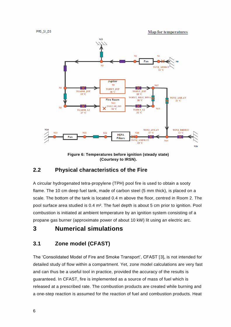
volume flow rates are given in Figure 5. The temperature map is given in Figure 6. The

experimental data are provided “as is” with no assumption. The experimental data

presented are some average values between -60 to 0 s (ignition) for the PRS-SI-D3

test. The density of air is assumed as constant equal at 1.18 kg/m³ to calculate the

x_EW

x_NS

5

relative total pressure. The uncertainties concerning the pressure and flow rate

measurements were evaluated about ± 30% [14].

Figure 4: Map for nodes ‘N’, branches ‘B’ and pressure sensors ‘P’ (Courtesy to IRSN).

Figure 5: Relative total pressures and air flow rates before ignition (steady state)

(Courtesy to IRSN).

6

Figure 6: Temperatures before ignition (steady state)

(Courtesy to IRSN).

2.2 Physical characteristics of the Fire

A circular hydrogenated tetra-propylene (TPH) pool fire is used to obtain a sooty

flame. The 10 cm deep fuel tank, made of carbon steel (5 mm thick), is placed on a

scale. The bottom of the tank is located 0.4 m above the floor, centred in Room 2. The

pool surface area studied is 0.4 m². The fuel depth is about 5 cm prior to ignition. Pool

combustion is initiated at ambient temperature by an ignition system consisting of a

propane gas burner (approximate power of about 10 kW) lit using an electric arc.

3 Numerical simulations

3.1 Zone model (CFAST)

The ‘Consolidated Model of Fire and Smoke Transport’, CFAST [3], is not intended for

detailed study of flow within a compartment. Yet, zone model calculations are very fast

and can thus be a useful tool in practice, provided the accuracy of the results is

guaranteed. In CFAST, fire is implemented as a source of mass of fuel which is

released at a prescribed rate. The combustion products are created while burning and

a one-step reaction is assumed for the reaction of fuel and combustion products. Heat

7

transfer in walls can be accounted for by solving the heat conduction equation normal

to the wall.

The following parameters have been set, in agreement with Figures 5 and 6:

Ambient Conditions – interior

Gas and wall temperature 34 °C

Thermodynamic pressure 98384 Pa

Relative humidity 50 %

Ambient Conditions – exterior

Temperature 31 °C

Pressure 98300 Pa

The geometry consists of Room 1, Room 2, Room 3 and the corridor as seen in Figure

1. Room 2 is the fire room. All rooms are modelled because leakages towards these

rooms and subsequently towards the outside are included. The walls consist of 0.3 m

thick concrete, the ceiling is 0.05 m thick THERMIPAN (Table 1) and the floor is

concrete with a thickness of 1 m. Surface connections are used for each wall. The

rooms have normal flow characteristics; the corridor is modelled as ‘default Corridor’.

Leakage paths must be specified in compartments with closed doors and windows

during the fire event since zone fire models assume that compartments are completely

sealed unless otherwise specified. In reality, the resulting pressure and the rate of

pressure rise are often kept very small by gas leaks through openings in the walls and

cracks around doors, known as “leakage paths.” By contrast, compartments with at

least one open door or window can maintain pressure close to ambient during the fire

event.

All the leakages due to penetrations and cracks have been modelled here as a

0.003 m² gap (0.003 m x 1 m) underneath the doors (horizontal flow vents). This gap

has been chosen such that the calculated pressure variation matches the

experimentally measured value.

The ventilation system is assumed to continue to operate during the fire with no

changes brought about by fire-related pressure effects. It is modelled as a constant

renewal rate of 180 m³/h. The description of the fan includes a drop off in flow beginning

at a pressure specified at 2000 Pa. Above this pressure drop, the flow gradually drops to

zero flow (4000 Pa). CFAST does not include provisions for reverse flow through a fan.

The fuel is TPH, a combustible liquid, specified as follows:

Heat of combustion ΔHc = 4.2x107 J/kg

8

Heat of Gasification 361 kJ/kg

Volatilization temperature 188 °C

Radiative fraction 0.35

Molar mass 0.17 kg/m³

Total mass 14.6 kg

H/C 0.1806

CO/CO2 and C/CO2 As in experiment

Lower Oxygen Limit 10 %

Gaseous ignition temperature 53.5 °C

Ignition criterion Time = 0s

The Mc Caffrey plume model [7] is used.

3.2 Field model ISIS

ISIS is an open source CFD (Computational Fluid Dynamics) package developed by

IRSN [4]. It is based on the scientific computing development platform PELICANS and

available as open-source software (https://gforge.irsn.fr/gf/project/pelicans). It is

entirely parallized via this platform, for both the assembly and solution of discrete

systems.

The governing equations describing the turbulent reactive flow in low Mach number

regime encompass the Favre-averaged Navier-Stokes equations (mass and

momentum). Turbulence is modelled by a modified k-ε model, using the Boussinesq

hypothesis for the buoyancy source terms in the transport equations for k and ε [8].

The EBU model is used for combustion.

The radiative heat transfer equation for an absorbing and emitting medium is solved

using the Finite Volume Method [9]. In addition, the effect of soot on the absorption

coefficient is taken into account by means of a correlation proposed by Novozhilov

[10]. Soot production is modelled on the basis of an average yield, ys= 0.11 kg/kg (kg

soot per kg fuel), as measured during the experiment. Soot is transported by

convection and diffusion.

An interesting feature concerns the calculation of the thermodynamic pressure in the

room. This calculation is based on a simplified momentum balance equation for the

system composed of the confined compartment and the ventilation network. A general

Bernoulli equation describes each branch i of the network, which is, in this particular

case, connected to the compartment (pipe-junction boundary condition):

9

fPPt

Q

S

Linodeth

i

i

i

, (1)

where Li and Si are respectively the length and the cross-sectional area of branch i, Qi

is the flow rate in branch i, Pnode,i is the pressure at extremity of the branch which is not

located at the compartment wall and f is an aerodynamic resistance:

i

i

QRQsignf (2)

The flow exponents are set to α = 2 and β = 1.

If the pipe length L is not specified, which is the case here, the stationary Bernoulli

equation:

fPP inodeth , (3)

is supplemented by the overall mass balance equation of the compartment:

i

ith QRT

WP

t0 (4)

Geometric and material properties as used are gathered in the following tables:

Air properties

Laminar viscosity Sutherland viscosity law,

μ0 = 1.68 x 10-5 Pa.s, T0 = 273 K, S = 110.5 K.

Specific heat capacity Cp = 1020 J/(kg.K)

Reference temperature Tref = 307 K

Turbulent Prandtl Pr = 0.7

Density Ideal Gas Law for low Mach number flows (P0 = 98384 Pa)

Turbulent Schmidt Sc = 0.7

Absorption coefficient Gas-soot mixture, gas coefficient 0.1/m, soot coefficient

1264/m/K. Soot density = 1800 kg/m³

The standard gravity field is applied.

Fuel properties

Heat of combustion ΔHc = 4.2x107 J/kg

Boiling point Tfuel = 461 K

The fuel is treated as dodecane with incomplete combustion: C12H26 + (18.5 - s) O2 +

N2 13 H2O + (12 - s) CO2 + N2 + sC with s=1.55833. s can be estimated from the

data of Tewarson [11] (ys ≈ 0.15) or from the experiment ys ≈ 0.11; ys = s*Wc/Wfuel =

s*12/170.

Initial conditions

10

Velocity 0.0 0.0 0.0 m/s

Gas and wall temperature T0 = Tref = 307 K

Thermodynamic pressure P0 = Pref + Plocal = 98384 Pa

Turbulence kinetic energy k0 = 1.E-6 m²/s²

Dissipation rate of

turbulent kinetic energy

ε0 = 1.E-9 m²/s³

Mixture fraction 0.0

Fuel mass fraction 0.0

Boundary conditions

At the inlet and exhaust openings, the pipe-junction boundary condition presented

above is used. The air flow resistances have been derived from the pressures

measured at the extremity of each branch in steady state conditions prior to ignition

(see Figure 5 and Figure 6): with Pinlet = 270 Pa (at 27°C) and Poutlet = -676 Pa (at

32°C), equation (2) yields Rinlet = 46445.1 m-4 and Routlet = 197142.1 m-4.

With the knowledge of the average branch velocity u inlet, and the setting of the

turbulent intensity i and the mixing length scale l, the turbulent kinetic energy k inlet and

the dissipation rate of the turbulent kinetic energy ε inlet are set at the boundary [12].

The turbulent intensity is set at 0.01 and the mixing length scale to 0.03 m.

At the pool surface, the experimentally measured burning rate, )(tmc , is used to

determine the inlet velocity: pfuel

cfuel

S

tmwnv

)( , along with the following conditions:

H = cp (Tfuel – T0) + ΔHc,eff , Yf = Z = 1.

Yf = Z = H = 0

If )(tmc >0

otherwise

ρ = ρ(Tfuel) = 4.14 kg/m³ P0 = Pref + Plocal = 983 hPa + Plocal

Turbulence kinetic energy kpool = 1.E-5 m²/s²

Dissipation rate of turbulent kinetic energy εpool = 1.E-9 m²/s³

A gray-surface boundary condition is applied for the radiative intensity, with pool

surface emissivity equal to 1. The fuel inlet temperature is set at boiling temperature

(461K) and the pool wall is assumed to be adiabatic.

The heat transfer to the concrete walls and THERMIPAN ceiling are calculated with

the wall law [18]. The conditions were set as in Table 1, with exception of the

emissivity of the concrete wall, which is set to 0.9. The boundary condition with the

exterior is assumed to be adiabatic. The admission and extraction ventilation branches

are modelled as adiabatic.

11

Mesh characteristics and grid convergence

Grid sensitivity is important in the verification process of the numerical simulation

results. The grid convergence for a certain quantity can be influenced by the choice of

the time step and discretization schemes [13]. Therefore, a number of mesh/time step

studies have been performed, confirming that the grid is adequate (successive

reductions in mesh cell size hardly modify the results under consideration). Table 2

summarizes the grid characteristics while Figure 7 provides a graphical impression.

Name Ncells ΔxpoolΔypoolΔzpool ΔxmaxΔymaxΔzmax Δxwall,

Δywall Δzceiling

M6 46x56x40

= 103040 4.0x4.0x5.7 18.8x18.8x14.3 6 18 6 9

Table 2: Grid characteristics (number of cells ‘Ncells’ ; grid sizes ‘Δ' in cm ; ‘’: evolution

in the grid size near the objects mentioned).

Figure 7; +x_NS, +x_EW, +Z and 3D mesh clips. Only 1/4th

of the symmetrical mesh is

shown.

4 Quantification of comparison of results

12

In order to quantify differences between model predictions and experimental

measurements, much effort has recently been carried out to develop the application of

metric operators. The reader is referred to a PRISME group publication [14], where a

discussion is given on several metric operators for the case of a pool fire scenario in a

well-confined compartment.

The simplest option is the single-point comparison, which can be used to quantify

differences between measurements and numerical results for (scalar) quantities that

are independent of time and space, or to compare point wise peak values from fire

experiments and model predictions:

E

EM (5)

where E represents the experimental observation and M the model prediction.

A normalized relative difference can be used [15] if one wants to take into account the

initial state of the calculation as a reference state or to avoid any discussion about

units:

0

00

EE

EEMM

E

EM

p

pp

(6)

where ΔM is the difference between the peak value (Mp) of the model prediction and

the ambient value (M0), and ΔE is the difference between the experimental observation

(Ep) and the ambient value (E0).

A general formulation for the single-point comparison using peak values (e.g.

temperature, over- or under-pressure, critical oxygen value in the compartment, etc.),

named Local Error, can be written as:

i

ii

e

em

max

maxmax or

i

ii

e

em

min

minmin (7)

where Δmi = mi-m0 and Δei = ei-e0 with mi and ei the ith values of the vector m and e

respectively.

In order to obtain an overall comparison of two curves, the single-point comparison

can be extended to multiple points. Each of these curves can be represented as a

multidimensional vector, with each point in time defining an additional dimension. For

simplicity, the analysis presented treats time-dependent quantities either averaged in

space or measured at a point. Prior to quantification of the differences, the data is

interpolated to a common time discretization (here 4s was used). The difference in the

overall magnitude of two vectors is calculated by the normalized Euclidean distance

between two vectors, termed Global Error:

13

2

1

2

1

n

i i

i

n

i

i

m Em E

E E

(8)

If the Euclidean Distance is zero, both vectors are identical.

To compare the shapes of the two curves, the cosine of the normalized inner product

of the vectors E and M is calculated.

yx

yxyx

,

,cos (9)

When the cosine equals 1, both curves can differ from each other only by a constant

multiplier.

Below, the results are evaluated using these three quantities.

5 Numerical simulation results: discussion

5.1 Burning Rate

As first part of the code testing, results in circumstances of oxygen deficiency are

investigated. The burning rate is an important boundary condition of the problem.

One option is to impose the burning rate as measured in the experiments. This curve

is labelled ‘MLR-exp’ in Figure 8. Results with this curve as input are labelled ‘MLR-

exp’ below.

Another option is to consider the mass-loss-rate (MLR) curve as determined in a free

atmosphere as input. This is common practice in calculations by fire safety engineers,

implicitly assuming that the model in the simulations will deal with circumstances of

oxygen deficiency and radiative feedback effects towards the flaming region. The input

curve is labelled ‘MLR-exp-free-atm’ in Figure 8. Results with this curve as input are

labelled ‘MLR-exp-free-atm’ below.

The burning rate evolution in the confined ventilated compartment versus time follows

the curve in free atmosphere quite well during the first three minutes. After about 200s,

the burning rate becomes higher in the compartment than in free atmosphere, most

probably due to radiative heat feedback from the flames to the fuel. After 5 minutes,

the fire starts to extinguish. Complete extinction is achieved after about 6 minutes.

ISIS

With the version of ISIS used here, however, solely the effect of oxygen deficiency on

the mass loss rate can be taken into account, using the Peatross - Beyler correlation

[16]:

14

1.11020 OXmm (10)

with 0m the burning rate (kg/s) for a fire in 21vol% oxygen concentration and X O2 the

mean oxygen mole fraction in a region near the flame. The region for averaging the

oxygen molar fraction XO2 was chosen as a cube of 1 m² surface area and 0.4 m height

around the burner. Averaging the oxygen mole fraction over a larger volume (e.g. the

‘whole domain’) negatively affects the results.

Expression (10) cannot predict a higher burning rate within the compartment than in

free atmosphere. Therefore, the observation in the period 200s – 300s cannot be

captured. This is clearly seen in Figure 8: the evolution is almost perfect during the

first 200s. After that, the MLR-exp curve cannot be followed. For obvious reasons,

burning afterwards (after 360s) lasts longer than in the MLR-exp curve, since the fuel

is consumed less rapidly. Despite this deficiency, the free atmosphere burning rate as

input, in combination with the Peatross - Beyler (‘PB’) correlation (10), is used in the

following sections.

Incorporation of effects of both lack of oxygen and radiative feedback is work-in-

progress [17], but this is beyond the scope of the present paper.

Figure 8: Measured burning rate in the compartment (‘MLR-exp’) or in free atmosphere

(‘MLR-exp-free-atm’) and calculated from ISIS (‘near flame region’ either a cube of

1 x 1 x 0.4m3 or ‘whole domain’). Input for the simulations is ‘MLR-exp-free-atm’.

CFAST

Fires in CFAST are defined as a series of individual fire objects which are then placed

as desired within compartments in the simulation. Each fire object defines the time

15

dependent variables of the fire which are the mass loss rate, rate of heat release, fuel

height, and fuel area. In the CFAST model, if sufficient oxygen is available, then fuel is

fully burned as [3]:

Where E is the heat release per mass unit of oxygen consumed, taken to be 1.31 x 107

J/kg (based on oxygen consumption calorimetry for typical fuels) and neededOactualO mm ,, ,

the oxygen needed to achieve full combustion.

However, if the oxygen concentration is low enough, a limit of burning due to oxygen

depletion is incorporated by limiting the burning rate as the oxygen level decreases

until a “lower oxygen limit” (LOL) is reached. To limit the actual burning which takes

place in the combustion zone, the following model is incorporated:

availableOneededOactualO mmm ,,, ,min (12)

The lower oxygen limit is incorporated through a smooth decrease in the burning rate

near the limit:

LOLOeavailableO CXmm2,

(13)

where em is the mass entrainment flow rate, XO2 is the mass fraction of oxygen, and

the lower oxygen limit coefficient, CLOL, is the fraction of the available fuel which can

be burned with the available oxygen and varies from 0 at the limit to 1 above the limit.

By concept, em and XO2 are calculated for each zone in CFAST, i.e. the lower layer,

the upper layer and the vent flow. In each zone, the heat release, originating from the

pyrolysis rate of the source or unburned hydrocarbons of previous regions, is limited

by the available oxygen in that region.

The curve labelled ‘MLRmCFAST-free-atm+LOL12’ in Figure 9 shows the effect of

using a lower oxygen value of 12% on the MLR-exp-free-atm input. At a time of 5.3

minutes, the oxygen drops below 12% and the MLR is consequently lowered.

The investigation of altering the LOL value is shown in Figure 9. If a very low LOL

value is used (e.g. 1%, i.e. ‘LOL1’), the input curve of MLR will be tracked unaltered by

CFAST. Because it is desired that the MLR-exp stays unaffected (it is a measured

value inside the compartment), a LOL of 1% is further used. A LOL of 10% or 12%

seems adequate to be used with MLR-exp-free-atm due to the fact that these values

produce the lowest Global Error and best Cosine values (Figure 10) for the MLR

prediction. With a LOL of 14%, the MLR drops too soon.

When the simulations reach the lower oxygen limit, the burning rate is limited as

described above. Due to this lowering of burning rate, the loss of heat becomes larger

C

actualOH

Exmm

, (11)

16

than the addition of heat, leading to the lowering of pressure. In turn, the admission of

fresh air is possible again, leading to a disturbance (uppercut) in mass loss rate for the

CFAST simulations.

Figure 9: Measured burning rate in the compartment (‘MLR-exp’) or in free atmosphere

(‘MLR-exp-free-atm’) and calculated from CFAST for different LOL. (MLR-exp-free-atm

overwritten with MLRmCFAST-free-atm+LOL1).

0

0.1

0.2

0.3

0.4

0.5

0.6

0.7

0.8

0.9

1

Global Error Cosine

LOL 14 LOL 12 LOL 10 LOL 1

Figure 10: Global Error and Cosine (0-500s) for different LOL in CFAST

(MLR-exp-free-atm response).

For completeness, the quantitative comparison of above mentioned simulation results

is shown in Table 3. The Local and Global Errors and the Cosine of the angle between

the vectors are reported for the MLR responses of the simulations with ‘MLR-exp-free-

atm’ as input.

In the following sections, the ‘MLRmCFAST+LOL1’ is used in CFAST in case of

analysis based on the mass loss rate as measured inside the compartment (can be

shortened ‘MLR-exp’ as it is basically the same). In ISIS, no Peatross & Beyler

17

correlation is used in this case. This choice is made when it is desired that both codes

track unaffected the MLR-exp curve as measured inside the compartment.

ISIS + Peatross –

Beyler (1x1x0.4) CFAST + LOL 12%

Time

frame (s)

Local

Error

Global

Error

cosine Local

Error

Global

Error

cosine

0-100 -0.00 0.07 0.998 0.02 0.06 0.998

100-250 -0.25 0.18 0.985 -0.22 0.16 0.988

250-450 0.37 0.930 0.48 0.881

0-500 -0.25 0.30 0.953 -0.13 0.37 0.930

Table 3: Quantitative comparison for MLR responses by the code with the mass-loss-

rate (MLR) curve as determined in a free atmosphere ‘MLR-exp-free-atm’ as input. Local

Errors are determined for the maximum values of the curves.

5.2 Total derivative room pressure and the ventilation flow

rate

Room pressure may be important when it contributes to smoke migration to adjacent

compartments. It is also a major concern when dealing with dynamic confinement to

minimize the contamination propagation in nuclear facilities. Together with the total

relative pressure, volume flow rate at the admission and extraction branches of the

ventilation network describe the aeraulic behaviour of the fire room and the effects on

the ventilation network during the fire. These attributes can also be important because

it influences the outcome of under ventilated fires. Both CFAST and ISIS calculate

room pressure as they solve energy and mass balance equations in the control

volume. CFAST requires the volume flow rate at the branches as an input. A change in

flow rate can be defined in CFAST with a description of a fan or the change of the

initial opening fraction of a mechanical vent at a certain time during the simulation.

CFAST does not include provisions for reverse flow through a fan. The ISIS model

provides a boundary condition which can be used in the case of a confined

compartment connected to a ventilation network (section 3.2). The particular modelling

takes into account pressure variations over time inside the fire compartment.

ISIS

Figure 11 shows the measured versus predicted pressures in t ime by ISIS. The

measured pressure has an expanded uncertainty of ± 2% [14]. ISIS predicts the

pressure behaviour very well with MLR-exp as an input. The reproduction of pressure

variations are important for the nuclear safety and are qualitatively recovered by ISIS.

18

Figure 11: Calculated vs measured total relative pressure in the fire room

(measuring range: -7000 … 10 000 Pa). Xm = ISIS prediction

Further, roughly no difference in pressure prediction is observed during the first 200s

due to the consistent MLR-exp and MLR-exp-free-atm. Between 200s and 320s, MLR-

exp-free-atm is smaller, resulting in less pressure rise (due to less heating). When

applying the MLR-exp-free-atm, the fire keeps on burning after 370s because the code

does not predict the extinguishment. As a result, heating still occurs, resulting in a

higher pressure than when applying MLR-exp. These effects are also visible in the

quantitative comparison (Table 4). The errors between measured and calculated

pressure rise with time for MLR-exp-free-atm as input. This shows that the MLR

greatly affects the pressure behaviour inside the compartment.

Additionally, the above shows that it is important to consider the extinction phase of a

fire and the cooling down of the compartment within the safety analyses concerning

pressure confinements. In general, the occurring negative pressure can be explained

due to the larger loss of heat through the walls and vents than the heat generated by

the fire in the compartment.

In order to validate the ISIS pipe-junction boundary condition, considerations of

pressure and volume flow rate at the admission and extraction branches of the

ventilation network are regarded (Figure 12). As could be expected, errors for volume

flow rate (Table 5 and Table 6) are larger for MLR-exp-free-atm than for MLR-exp

because of the larger error for MLR-exp-free-atm (0-500s). A differentiation in errors

can be noticed between the prediction of the volume flow at admission and extraction

19

branch. Before extinguishing of the fire, the Global Error is smaller for the extraction.

The comparison for the extraction volume flow rate has even so a Cosine value closer

to 1, resulting in a better performance of the boundary condition for the extraction. The

somewhat to high predicted reverse flow through the admission seems to cause the

small under prediction of the first and second pressure peak (Table 4). Nonetheless,

the results evidence the used boundary condition is capable of modelling the in- en

outlet branch.

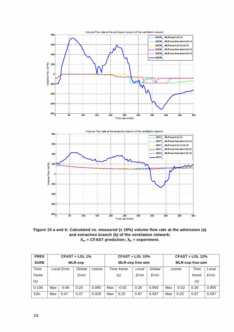
Figure 12 a and b: Calculated vs. measured (± 10%) volume flow rate at the

admission (a) and extraction branch (b) of the ventilation network;

Xm = ISIS prediction, XE = experiment.

20

PRESSURE ISIS

MLR-exp

ISIS + Peatross – Beyler

(1x1x0.4) MLR-exp-free-atm

Time frame

(s)

Local Error Global

Error

cosine Local Error Global

Error

cosine

0-100 Max -0.10 0.10 0.995 Max -0.12 0.13 0.993

100-250 Max -0.15 0.13 0.992 Max -0.16 0.53 0.850

250-450 Min 0.07 0.15 0.988 Min -0.67 0.72 0.854

0-500 0.13 0.992 0.51 0.868

Table 4: Quantitative comparison for PRESSURE between experimental data and the

response by the ISIS code with the MLR curve ‘MLR-exp’ or ‘MLR-exp-free-atm’ as input.

Q-ADM ISIS

MLR-exp

ISIS + Peatross – Beyler

(1x1x0.4) MLR-exp-free-

atm

Time

frame

(s)

Local Error Global

Error

cosine Local Error Global

Error

cosine

0-100 Max 0.00 0.36 0.944 Max -0.02 0.30 0.958

100-250 Max -0.21 0.21 0.977 Max -0.16 0.55 0.835

250-450 Min 0.32 0.34 0.983 Min -0.19 0.29 0.965

0-500 0.32 0.966 0.37 0.930

Table 5: Quantitative comparison for Volume Flow at the admission branch between

experimental data and the response by the ISIS code with the MLR curve ‘MLR-exp’ or

‘MLR-exp-free-atm’ as input.

Q-EXT ISIS

MLR-exp

ISIS + Peatross – Beyler

(1x1x0.4) MLR-exp-free-

atm

Time

frame

(s)

Local Error Global

Error

cosine Local Error Global

Error

cosine

0-100 Max -0.01 0.13 0.993 Max -0.03 0.11 0.995

100-250 Max -0.16 0.14 0.998 Max -0.13 0.24 0.980

250-450 Min 0.38 0.42 0.918 Min -0.63 0.68 0.731

0-500 0.24 0.972 0.37 0.930

Table 6: Quantitative comparison for Volume Flow at the extraction branch between

experimental data and the response by the ISIS code with the MLR curve ‘MLR-exp or

‘MLR-exp-free-atm’ as input.

CFAST

21

The pressure evolution observed for the different simulations shown in Figure 13

confirm that for MLR-exp, the LOL must be set on a low value (<10% as found in

section 5.1). This seems consistent with impact of the MLR response on the pressure

and supports the tracking the MLR-exp curve. Recall that for ‘MLR-exp-free-atm’ as

input, the MLRmCFAST-free-atm response showed the best results for a LOL of 10%

or 12%. This LOL values are confirmed when regarding the pressure behaviour.

Visually, one can discuss which LOL to use, but on the basis of the quantitative

comparison (Table 7), it can be concluded that using a LOL of 10% gives the best

prediction of the pressure curve. It is therefore decided to further use a LOL value of

10% when using ‘MLR-exp-free-atm’ as input.

In order to validate the admission and extraction boundary condition available in

CFAST, the pressure and volume flow rate at the admission and extraction branches

of the ventilation network are examined (Figure 15 a and b). Fresh air intake trough

the admission is blocked between 30s and 270s, showing clearly the inability of

CFAST to model reversed flows at admission. Air leaves the fire room mainly through

the small gaps under the doors (Figure 14). Because the aeraulic resistance of those

gaps does not match the true aeraulic resistance as in the experiments, the pressure

and the flow rates cannot be predicted accurately at the same time. The extraction

condition in CFAST is not capable of capturing a more intense outflow due to the

internal pressure rise. In the experiment, newly fresh air enters in the compartment at

about 270s, due to a pressure evolution in the compartment towards ambient

pressure. At this point in time, cold air enters the compartment, which results in a

pressure drop. Subsequently, the heat of the fire heats up this air, resulting in a

pressure rise. After about 270s, also the flow rates through the gaps under the door

are responsible for the pressure prediction. In general, the volume flow rate in and out

the compartment through the admission and extraction are badly predicted by CFAST.

Additionally, it can clearly be seen that the MLR mainly determines the pressure

behaviour and that absolute values for pressures are mostly affected by creating gaps

under the doors. A quantitative comparison confirms this statement (Table 8 and Table

9). For CFAST, it is also clear within the quantitative comparison that the prediction is

somewhat better for the extraction branch, here certainly due to the inability of CFAST

to predict reverse flow. Consequently, it is expected that smoke concentration,

interface heights and even temperatures will be affected by this behaviour.

It appears that CFAST is able to predict the pressure time curve quite well when

compared to ISIS (Table 4 vs.Table 7), and this in order to make safety evaluations

related to pressure inside the compartment. The former is true for completely open

simulations, but recall that the leakage (gap under the doors) in the CFAST simulation

22

was chosen “ad hoc”, (even if it seems realistic) so that the calculated pressure

resembles the measured pressure. With the measured MLR inside the compartment

(e.g. MLR-exp) as input, CFAST was able predict the right shape of the pressure, but

absolute values were hard to determine if one does not have any experimental data.

Above observation is in contrast with the ISIS code, where no gaps were assumed and

the pipe-junction boundary condition was able to predict adequately the pressure

inside the compartment (Figure 11). This illustrates the interest of thermodynamic

pressure modelling of equation (1) and (4).

Figure 13: CFAST - Calculated (± 75%) vs measured (± 2%) total relative pressure

in the fire room (measuring range: -7000 … 10 000 Pa). Xm = CFAST prediction

23

Figure 14: Calculated Volume Flow rate through the 3 gaps under the fire room doors

24

Figure 15 a and b: Calculated vs. measured (± 10%) volume flow rate at the admission (a)

and extraction branch (b) of the ventilation network;

Xm = CFAST prediction; XE = experiment.

PRES

SURE

CFAST + LOL 1%

MLR-exp

CFAST + LOL 10%

MLR-exp-free-atm

CFAST + LOL 12%

MLR-exp-free-atm

Time

frame

(s)

Local Error Global

Error

cosine Time frame

(s)

Local

Error

Global

Error

cosine Time

frame

(s)

Local

Error

0-100 Max -0.06 0.20 0.980 Max -0.02 0.30 0.955 Max -0.02 0.30 0.955

100- Max 0.07 0.37 0.929 Max 0.25 0.87 0.597 Max 0.25 0.87 0.597

25

250

250-

450

Min 0.06 0.18 0.987 Min 0.19 0.54 0.844 Min 0.26 1.15 0.319

0-500 0.24 0.971 0.56 0.834 0.793 0.675

Table 7: Quantitative comparison for PRESSURE between experimental data and the

response by the CFAST code with the MLR curve ‘MLR-exp’ or ‘MLR-exp-free-atm’ as

input.

Q-

ADM

CFAST + LOL 1%

MLR-exp

CFAST + LOL 10%

MLR-exp-free-atm

CFAST + LOL 12%

MLR-exp-free-atm

Time

frame

(s)

Local Error Global

Error

cosine Local Error Global

Error

cosine Local Error Global

Error

cosine

0-100 Max -1.00 0.99 0.127 Max -1.00 0.99 0.122 Max -1.00 0.99 0.122

100-

250

Max -1.00 1.01 -0.217 Max -1.00 1.06 -0.761 Max -1.00 1.06 -0.761

250-

450

Min -0.75 0.69 0.945 Min -0.75 0.79 0.898 Min -0.75 0.85 0.685

0-500 0.85 0.668 0.91 0.561 0.92 0.524

Table 8: Quantitative comparison for Volume Flow at the admission branch between

experimental data and the response by the CFAST code with the MLR curve MLR-exp’ or

‘MLR-exp-free-atm’ as input.

Q-

EXT

CFAST + LOL 1%

MLR-exp

CFAST + LOL 10%

MLR-exp-free-atm

CFAST + LOL 12%

MLR-exp-free-atm

Time

frame

(s)

Local Error Global

Error

cosine Local Error Global

Error

cosine Local Error Global

Error

cosine

0-100 Max -0.59 0.60 0.951 Max -0.59 0.60 0.952 Max -0.59 0.60 0.952

100-

250

Max -0.66 0.64 0.982 Max -0.66 0.65 0.985 Max -0.66 0.65 0.985

250-

450

Min -1.34 1.00 0.255 Min -1.35 0.98 0.296 Min -1.37 1.00 0.279

0-500 0.72 0.758 0.71 0.777 0.72 0.760

Table 9: Quantitative comparison for Volume Flow at the extraction branch between

experimental data and the response by the CFAST code with the MLR curve MLR-exp’ or

‘MLR-exp-free-atm’ as input.

5.3 Oxygen concentration

Oxygen concentration is not an important attribute for nuclear fire safety analysis “as

such”, but it is essentially important as it may influence the outcome of fires in nuclear

facilities because of their compartmentalized nature. Oxygen has a direct influence on

the burning behaviour of a fire, especially if the concentration is relatively low (see

section 5.1). The CFAST two-zone model is able to predict oxygen concentration in

26

the upper and lower layers, and the ISIS model calculates the oxygen concentration in

each control volume defined in the computational domain.

ISIS

Figure 16 depicts the measured versus predicted oxygen volume concentrations in

time by ISIS. The measured oxygen concentration has an expanded uncertainty of ±

2 % [14]. ISIS predicts the oxygen concentration very well in the high region (HAUT)

and the region close to the flame base (FP), no matter if the input is ‘MLR-exp’ or

‘MLR-exp-free-atm’ (Table 10). In the lower region, outside the flame region (BAS), the

oxygen concentration drops sooner in the experiments, likewise as observed in the

high region. This behaviour is not captured correctly by the ISIS code. Nevertheless,

minimum oxygen concentration and oxygen rise after extinction is well captured.

27

Figure 16 a - c: Calculated (± 8%) vs. Measured (± 1%) O2 Volume concentration for the

sensors (a) O2FP (Z = 0.35 m: x_NS = -0.8 m; x_EW = 0),

(b) O2HAUT (Z= 3.3 m; x_NS = 1.5 m; x_EW = -1.25 m),

(c) O2BAS (Z= 0.8 m; x_NS = 1.5 m; x_EW = -1.25 m);

Xm = ISIS prediction, XE = experiment.

O2

ISIS

MLR-exp

ISIS + Peatross –

Beyler (1x1x0.4) MLR-

exp-free-atm

Time

frame 0 -

500s

Local

Error

Global

Error

cosine Local

Error

Global

Error

cosine

FP 0.12 0.06 0.998 0.06 0.05 0.999

HAUT 0.00 0.03 1.000 0.04 0.05 0.999

BAS 0.04 0.11 0.998 0.05 0.10 0.997

Table 10: Quantitative comparison for oxygen volume concentration between

experimental data and the response by the ISIS code with ‘MLR-exp’ or ‘MLR-exp-free-

atm’ as input.

Figure 17 depicts two sectional planes which visualise the oxygen mass fraction for

the MLR-exp simulation (see Figure 3). The higher oxygen region (red) can be

expected to dictate the oxidation of fuel (thus the burning). For this reason, a higher

oxygen region around the burner with an area 1 m² and 0.4 m height was then “ad

hoc” chosen as bounding area for averaging the oxygen molar fraction XO2 when using

the ‘MLR-exp-free-atm’, i.e. as measured in the free atmosphere as an input (see

section 5.1). The oxygen reduction via the Peatross & Beyler correlation resulted

subsequently in the MLR-exp-free-atm response.

28

Figure 17: Visualisation of the oxygen mass fraction at t=315s; YO in %

(plane left: x_EW = 0 m; plane right: x_NS = 0 m)

CFAST

For completeness, the Figure 18 depicts the result of predicted oxygen volume

concentration obtained by CFAST. Because of the two-zone principle of CFAST and

the fact that the upper layer descends very rapidly under 0.8 m, the sensor at the

bottom (“BAS”) is not shown on the figure. As could be expected by the inability to

capture reverse (in)flow in CFAST (Figure 15), the oxygen concentration is somewhat

underestimated: less fresh air enters the compartment in the simulations, compared to

the experiments.

Figure 18: Calculated (± 8%) vs. Measured (± 1%) O2 Volume concentration for the

sensor O2HAUT (Z= 3.3 m; x_NS = 1.5 m; x_EW = -1.25 m).

In addition, Table 11 provides the quantitative comparison for oxygen volume

concentration between experimental data and the response by the CFAST code with

the MLR curve ‘MLR-exp’ or ‘MLR-exp-free-atm’ as input.

O2 CFAST + LOL 1% CFAST + LOL 10%

29

MLR-exp MLR-exp-free-atm

Time

frame 0 -

500s

Local

Error

Global

Error

cosine Local

Error

Global

Error

cosine

HAUT -0.22 0.20 0.994 -0.34 0.22 0.992

Table 11: Quantitative comparison for oxygen volume concentration between test data

and the response by the CFAST code with the ‘MLR-exp’ or ‘MLR-exp-free-atm’ as input.

6 Extra Numerical ISIS experiments: sensitivity

analysis

The following sensitivity study is based on the input settings as described in paragraph

3.2 and only for MLR-exp. The simulation results of this reference case are shown in

paragraph 5.

6.1 Overview of the sensitivity performed

6.1.1 Soot production (ISIS)

Soot is a product of incomplete combustion and its formation is a complex

phenomenon, making it difficult to model. Nevertheless, soot is of importance in

thermal radiation models. Many approaches are available, but only two are restrained.

Fixed soot yield fraction

The reference simulation was set up with a fixed soot yield fraction ys of 0.11. This

value of soot fraction was based on the average of the soot measurement values for

the experiment. For a first sensitivity study, this fixed soot yield was set to 0.15 [11]

and the stoichiometric carbon coefficient of the dodecane combustion was

consequently changed. This higher value of soot fraction is set on the assumption that

quite some soot will be formed during the burning period. Due to this consideration, a

value of 0.15 would possible be used when considering this scenario for safety

analysis purposes.

Simulation IDs: M6_ys0.15_FVM1 vs. M6_ys011_FVM.

Modeling soot yield

1 This code means: mesh size and time step ‘M6’, ys = 0.15 and using FVM to calculate the

radiative heat transfer

30

The Moss two-equation model is used to model the soot production [18]. The variables

of the modal are:

- the soot mass fraction Ys,

- the soot particle concentration Xn [mol.kg−1].

This model takes into account the processes of nucleation, surface growth and

coagulation. The soot combustion term depends on a specific oxidation rate.

Moreover, a thermodiffusion is added to the equations.

The use of this model can be compared to the use of fixed soot yield modelling as

described above. Two sets of Moss-coefficients, which depend on the fuel, were used

(Cα, Cβ and Cγ); one set for Low Sooty (LS) flames and one set of Heavy Sooty (HS)

flames. The model constants used were ([18] and [19]):

LS: Cα = 1.7 x 108 m³kg-2K-1/2s-1 ; Cβ = 1.0 x 109 m³K-1/2s-1; and Cγ = 4.2 x 10-17 kg-2/3K-

1/2s-1

HS: Cα = 1.3 x 106 m³kg-2K-1/2s-1 ; Cβ = 2.0 x 109 m³K-1/2s-1; and Cγ = 8.5 x 10-13 kg-2/3K-

1/2s-1

For both simulations, the fuel is treated as dodecane incomplete combustion in air as

presented in paragraph 3.2.

Simulation IDs: M6_mossLS_FVM vs. M6_mossHS_FVM (vs. M6_ys0.15_FVM &

M6_ys011_FVM)

6.1.2 Radiation modelling

P1 vs. FVM

Using the P1 radiation model instead of the Finite Volume Method (FVM) is considered

[18]. Within the spherical harmonic approximation P1, radiation intensity is expressed

by means of 1 harmonic, while with FVM the total set of admissible directions of

propagation is discretized in a finite set of control angles characterize by the angular

coordinates of its direction. The P1 approximation is very accurate if the optical

dimension of the medium is large. However, it yields inaccurate results for thinner

media particular near the domain boundaries.

Simulation IDs: M6_ys0.11_P1 vs. M6_ys011_FVM

6.1.3 Wall emissivity

The emissivity of the wall is changed from 0.9 (soot deposits) to 0.7 (no soot deposits).

Simulation IDs: M6_ys0.11_FVM vs. M6_ys011_FVM_εw07

6.1.4 Turbulence modelling

31

Two-equation turbulence RANS models (k – ε and k - ε RNG) with buoyancy

modifications of the source terms can be employed in ISIS to predict turbulent

viscosity, characteristic length and time scale [18]. With RNG, the transport k-equation

remains the same as the standard k – ε model except for model constant.

Nevertheless, a modification to the ε equations is made, whereby an additional rate of

strain term is introduced. For weakly to moderate strained flows, the RNG k – ε model

tends to yield comparable results to the k – ε model. No rapid strain or streamline

curvature is expected, so results should be largely equal.

Simulation IDs: M6_ys0.11_FVM vs. M6_ys011_FVM_RNG

6.1.5 In- and output branch flow resistance

The pipe-junction boundary condition implemented in ISIS is intended to be applied in

the case of a confined domain which is connected to a ventilation network (1). The

sensitivity consists of changing the aeraulic resistance R of the network in order to

investigate the effects on the pressure. R is changed to 1.1R (+10%) to study the

behaviour for a larger flow resistance. The resistance is also changed to -10%, -30%

and -50% in order to investigate the behaviour when applying a more open boundary

condition.

Simulation IDs: M6_ys0.11_FVM_R+10%, M6_ys0.11_FVM_R-10%,

M6_ys0.11_FVM_R-30%, M6_ys0.11_FVM_R-50% vs. M6_ys0.11_FVM

6.2 Results of the sensitivity study

With the use of the pipe-junction boundary condition, the pressure inside the

compartment during a fire is adequately predicted. This boundary condition relies on

measured pressures, but only at steady state before ignition. Consequently, semi-blind

simulation can be made with some degree of confidence in pressure predictions.

Figure 19 and Figure 20 show the sensitivity analysis results for the pressure

predictions in the compartment.

32

Figure 19: Plot of Calculated vs. Measured Total Pressure sensitivity.

Figure 20: Plot of Calculated vs. Measured Total Pressure sensitivity for

change in- and outflow branch resistance.

These pressure responses are subsequently investigated through the use of the

metrics proposed in paragraph 4.

Figure 21 depicts the evolution in Global Error for the conducted sensitivity. It can be

concluded that the aeraulic resistance has the largest influence on the pressure

results. Because aeraulic resistance is calculated from pressure measurements, it

constitutes an error input for simulations. It is observed that an uncertainty of 10% on

the aeraulic resistance is acceptable for conducting simulations. Using open boundary

conditions for modelling the aeraulics seems unacceptable as from lowering the

33

resistance with 30%, the Global Error becomes larger than 30%. Further, it is

observed that soot modelling has a relatively strong influence on the Global Error and

is the only parameter which greatly affects the shape of the pressure curve (Figure

22). The soot yield fraction strongly determines the soot concentration, which in turn

affects the radiation heat transfer and subsequently gas and wall temperatures [20].

This explains changes in the pressure variation (through the ideal gas law). Preferably,

a fixed soot yield ys of 0.11 (mean value as measured during the experiment) is used.

Nevertheless, using the Moss-model to predict soot yield with low soot (LS) model

constants is useful and acceptable in an error range of 25%.

The results are less sensitive to changes in other model settings. The relative

importance of changing the radiation model, wall emissivity and turbulence modelling

can be seen in Figure 23 to Figure 25. Wall emissivity and radiation modelling affect

gas and wall temperatures [20], and thus subsequently the pressure evolution inside

the compartment. Using P1 approximation to solve the radiation or FVM does not

change Local Error for pressure predictions, even so as using the RNG k – ε model

instead of the unaltered ε equation. The third most important parameter seems thus to

be the wall emissivity. At the beginning of the fire, there are minor soot deposits on the

wall, such that an emissivity of 0.7 is more acceptable to use. As the fire starts to

extinguish, a wall emissivity of 0.9 seems more appropriate as can be seen by a lower

Local Error in pressure predictions after 250s.

Euclidean Pressure Global Error

0

0.1

0.2

0.3

0.4

0.5

P0-500

M6_ys0.11_FVM M6_ys0.15_FVM M6_ys0.11_P1M6_ys0.11_FVM_RNG M6_mossHS_FVM M6_mossLS_FVMM6_ys0.11_FVM_εw07 M6_ys0.11_FVM_R+10% M6_ys0.11_FVM_R-10%M6_ys0.11_FVM_R-30% M6_ys0.11_FVM_R-50%

Figure 21: Quantitative comparison via Global Error of pressure sensitivity

response (0-500s).

34

Euclidean Pressure cosine

0.7

0.8

0.9

1

P0-500

M6_ys0.11_FVM M6_ys0.15_FVM M6_ys0.11_P1M6_ys0.11_FVM_RNG M6_mossHS_FVM M6_mossLS_FVMM6_ys0.11_FVM_εw07 M6_ys0.11_FVM_R+10% M6_ys0.11_FVM_R-10%M6_ys0.11_FVM_R-30% M6_ys0.11_FVM_R-50%

Figure 22: Quantitative comparison via Cosine of pressure sensitivity response (0-500s).

Pressure Local Error Maximum

-0.6

-0.5

-0.4

-0.3

-0.2

-0.1

0

0.1

0.2

P0-100

M6_ys0.11_FVM M6_ys0.15_FVM M6_ys0.11_P1

M6_ys0.11_FVM_RNG M6_mossHS_FVM M6_mossLS_FVM

M6_ys0.11_FVM_εw07 M6_ys0.11_FVM_R+10% M6_ys0.11_FVM_R-10%

M6_ys0.11_FVM_R-30% M6_ys0.11_FVM_R-50%

Figure 23: Quantitative comparison via Local Error of maximum pressure sensitivity

response between 0 and 100s (first pressure peak).

Pressure Local Error Maximum

-0.6

-0.5

-0.4

-0.3

-0.2

-0.1

0

0.1

0.2

P100-250

M6_ys0.11_FVM M6_ys0.15_FVM M6_ys0.11_P1

M6_ys0.11_FVM_RNG M6_mossHS_FVM M6_mossLS_FVM

M6_ys0.11_FVM_εw07 M6_ys0.11_FVM_R+10% M6_ys0.11_FVM_R-10%

M6_ys0.11_FVM_R-30% M6_ys0.11_FVM_R-50%

Figure 24: Quantitative comparison via Local Error of maximum pressure sensitivity

response between 100s and 250s (second pressure peak).

35

Pressure Local Error Minimum

-0.4

-0.3

-0.2

-0.1

0

0.1

0.2

P250-450

M6_ys0.11_FVM M6_ys0.15_FVM M6_ys0.11_P1

M6_ys0.11_FVM_RNG M6_mossHS_FVM M6_mossLS_FVM

M6_ys0.11_FVM_εw07 M6_ys0.11_FVM_R+10% M6_ys0.11_FVM_R-10%

M6_ys0.11_FVM_R-30% M6_ys0.11_FVM_R-50%

Figure 25: Quantitative comparison via Local Error of maximum pressure sensitivity

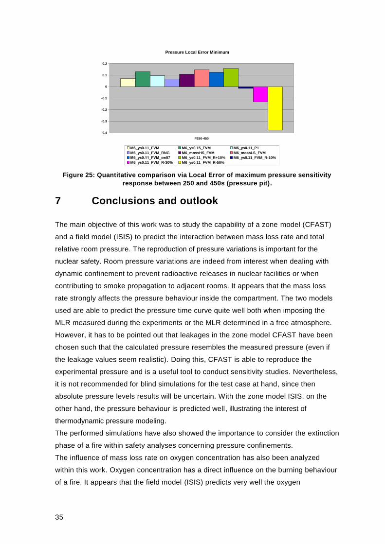
response between 250 and 450s (pressure pit).

7 Conclusions and outlook

The main objective of this work was to study the capability of a zone model (CFAST)

and a field model (ISIS) to predict the interaction between mass loss rate and total

relative room pressure. The reproduction of pressure variations is important for the

nuclear safety. Room pressure variations are indeed from interest when dealing with

dynamic confinement to prevent radioactive releases in nuclear facilities or when

contributing to smoke propagation to adjacent rooms. It appears that the mass loss

rate strongly affects the pressure behaviour inside the compartment. The two models

used are able to predict the pressure time curve quite well both when imposing the

MLR measured during the experiments or the MLR determined in a free atmosphere.

However, it has to be pointed out that leakages in the zone model CFAST have been

chosen such that the calculated pressure resembles the measured pressure (even if

the leakage values seem realistic). Doing this, CFAST is able to reproduce the

experimental pressure and is a useful tool to conduct sensitivity studies. Nevertheless,

it is not recommended for blind simulations for the test case at hand, since then

absolute pressure levels results will be uncertain. With the zone model ISIS, on the

other hand, the pressure behaviour is predicted well, illustrating the interest of

thermodynamic pressure modeling.

The performed simulations have also showed the importance to consider the extinction

phase of a fire within safety analyses concerning pressure confinements.

The influence of mass loss rate on oxygen concentration has also been analyzed

within this work. Oxygen concentration has a direct influence on the burning behaviour

of a fire. It appears that the field model (ISIS) predicts very well the oxygen

36

concentration both with the MLR measured during the experiments or the MLR

determined in a free atmosphere. On the other hand, the simulations performed with

the two-zone model (CFAST) showed limitations to predict the oxygen concentration

due to the inability to capture reverse flow.

To complete this work a sensitivity study has been performed for the field model.

Influence on the outputs of soot production, radiation modelling, wall emissivity,

turbulence modelling and branch flow resistance have been analyzed. The aeraulic

resistance is the most important parameter. The model for soot also has a relatively

strong influence, through the impact on the evolution of the temperature inside the

compartment. Further investigations on the influence of soot models would therefore

be interesting. In the same sense, heat losses from the compartment (and e.g. wall

emissivities) are also important issues to consider.

[1] ISO 17873, Nuclear facilities – Criteria for the design and operation of ventilation systems for nuclear

installations other than reactors, 1st edition (2004).

[2] Prétrel, H. and J.M. Such, Study based on large-scale experiments on the periodic instabilities of pressure and

burning rate in the event of pool fire in a confined and mechanically ventilated compartment, Third European

Combustion Meeting ECM (2007).

[3] W. P. Jones, R. D. Peacock, G. P. Forney, P. A. Reneke, CFAST – Consolidated Model of Fire Growth and

Smoke transport (version 6) – Technical reference guide, Technical Report NIST-SP-1026, National Institute of

Standards and Technology (Revision April 2009).

[4] Institut de Radioprotection et de Sûreté Nucléaire, ISIS 2.3.1 – Tutorial, Validation and Verification, IRSN

Publications (2011).

[5] Laurent Adouin, Hugues Prétrel, William Le Saux, Overview of the OECD PRISME PROJECT – Main

Experimental Results, 21th International Conference on Structural Mechanics in Reactor Technology (SMiRT 21),

2011

[6] Prétrel, H., Querre, P. and Forestier, M., (2005). Experimental Study Of Burning Rate Behaviour In Confined And

Ventilated Fire Compartments. Fire Safety Science 8: 1217-1228. doi:10.3801/IAFSS.FSS.8-1217.

[7] McCaffrey, B.J., “Momentum Implications for Buoyant Diffusion Flames,” Combustion and Flame 52, 149 (1983).

[8] SGDH – single gradient diffusion hypothesis in K. Van Maele and B. Merci, “Application of Two Buoyancy-

Modified k- Turbulence Models to Different Types of Buoyant Plumes”, Fire Safety Journal, Vol. 41 (2), pp. 122 -138

(2006)

[9] Institut de Radioprotection et de Sûreté Nucléaire, Resolution in ISIS of the Radiative Transfer Equation using the

Finite Volume Method, SEMIC-(2010)-067/DL Ind.1.

[10] V. Novozhilov. Computational fluid dynamics modeling of compartment fires. Progress in Energy and Combustion

Science, 27:611–666 (2001).

[11] Archibald Tewarson, Chapter 4 in The SFPE Handbook of Fire Protection Engineering, 3th Edition (2002).

[12] Yeoh, G.H and K.K. Yuen, Computational fluid dynamics in fire engineering: theory, modelling and practice.

Amsterdam: Elsevier. ISBN 978-0-7506-8589-4 (2009).

[13] Sam S.Y. Wang, Patrick J. Roche, Richard A. Schmals, Yafei Jia and Peter E. Smith, Verification and Validation

of 3D Free-surface Flow Models, ASCE ISBN 978-0-7844-0957-2. (2008).

[14] L. Audouin et.al., Quantifying differences between computational results and measurements in the case of a

large-scale well-confined fire scenario. Nuclear Engineering and Design 241 (2011).

37

[15] Verification and Validation of Selected Fire Models for Nuclear Power Plant Applications, Technical Report

NUREG-1824 and EPRI 1011999, U.S. Nuclear Regulatory Commission, Office of Nuclear Research (RES),

Rockville, MD, 2007, and Electric Power Institute (EPRI), Palo Alto, CA. (2007).

[16] Peatross, M. J. and Beyler, C. L., ”Ventilation effects on compartment fire characterization”, Fire Safety Scien ce

– Proceeding of the Fifth International Symposium, International Association for Fire Safety Science, (1997), pp 403-

414.

[17] S. Suard, A. Nasr, S. Mélis, J-P Garo, H. EL-Rabii, L. Gay and L. Audouin, Analytical Approach for Predicting

Effects of Vitiated Air on the Mass Loss Rate of Large Pool Fire in Confined Compartments, Fire Safety Science 10

IAFSS, (2011).

[18] Institut de Radioprotection et de Sûreté Nucléaire, ISIS 2.3.1 – Physical Modelling, IRSN Publication (2011).

[19] Guan heng Yeoh, Kwok Kit Yuen, Computational Fluid Dynamics in Fire Engineering, Theory, Modelling and

Practice, ELSEVIER. ISBN 978-0-7506-8589-4. (2009).

[20] Sylvain Suard, Sylvain Vaux and Laurence Rigollet, Fire Code Benchmark activities within the international

research project PRISME – discussion on metrics used for validation and on sensitivity analysis, SMirt 21, 2011