DOEINASA10394-1 NASA CR-174755

Computer Simulation 09 the Heavy- Duty Turbo=Compsoug?ded Diesel Cycle for Studies of Engine Efficiency and Perf ormanee

Dennis N. Assanis, Jack A. Ekchian, John 5. Heywood, and Kriss K. Replogle Sloan Automotive Laboratory Massachusetts lnstitue of Technology Cambridge, Massachusetts 021 39

May 1984

Prepared for NATllONAL AERONAUTICS AND SPACE ADMINISTRATION Lewis Research Center Cleveland, Ohio 441 35 Under Grant NAG 3-394

for U.S. DEPARTMENT OF ENERGY Conservation and Renewable Energy Office of Vehicle and Engine R&D Washington, D.C. 20585 Under Interagency Agreement DE-A101 -8QCS50194

https://ntrs.nasa.gov/search.jsp?R=19840025235 2020-02-10T12:31:29+00:00Z

Table of Contents

1 . INTRODUCTION

2. BASIC ASSUMPTIONS OF ENGINE MODEL

3. CONSERVATION EQUATIONS

3.1 Conservation of Mass 3.1 .1 Conservation of t o t a l mass 3.1 - 2 Conservation of fue l mss

3.2 Conservation of Energy

4. APPLICATION OF CONSERVATION EQUATIONS TO ENGINE PROCESSES

5. MODELLING OF ENGINE PROCESSES

5.1 Gas Exchange 5.2 Combustion Model 5.3 Ignition Delay Model 5.4 Heat Transfer 5.5 Twbulent Flow Model 5.6 Engine Friction Model

6. BASIC ASSWTIONS OF OTHER COMPONENT MODELS

7. MODELLING OF SYSTEM COMPONENTS

7.1 State Variables 7.2 Derivation of Different ial Equations

7.2.1 Manifolds 7.2.2 Turbocharger

7.3 Wastegate and EGR Valve Models 7.4 Intercooler Model 7.5 Manifold geat Transfer 7,6 Pressure Loss=

8. THERM3DYNAMIC PROPERTIES

9. TRANSPORT PROPERTIES

1 0. ITERATION PROCEDURE

10.1 Method of Solution 1 0.2 Crank Angle by Crank Angle Integration

$.PaC@DmG PAGE BLAiNF; B E T

iii

1 1 . PROGRAM INPUTS AND OUTPUTS

11.1 Inputs 1 1 . l . 1 Eng ine operating condit ions 1 1 . l . 2 System dimensions and design parameters 11.1.3 Heat t rans fe r and turbulent flow

parameters 1 1 .1 .4 Engine f r i c t i o n parameters 11.1.5 I n i t i a l condit ions 11.1.6 Ambient condit ions 1 1 . l . 7 Cornputat ional pararn? ters

1 1.2 Turbocharger and Power Turbine Maps 11.3 outputs

11 .3.1 Input echo 11.3.2 Main crank angle by crank angle r e s u l t s 1 1.3.3 Integrated r e s u l t s and cycle performnce 1 1 .3.4 Sub-mdpl r e s u l t s

1 . INTRODUCTION

The u s of ceramics in heavy duty d iese l engine applications is

especially promising [1 1. It has been shown in the TACOM/Cmins Adiabatic

Engine Program tha t reductions in heat losses at appropriate points i n the

diesel engine system re su l t i n substantially increased exhaust enthalpy [ 2 ] .

One of the mst promising concepts for taking advantage of t h i s increased

exhaust enthalpy is the turbocharged turbo-compounded d iese l engine cycle C31.

This engine concept consis ts of several sub-systems: compressor, engine,

turbocharger turbine , compounded turbine , ducting and heat exchangers.

Applications of ceramic materials t o d i f fe ren t sub-system components have

widely different degrees of d i f f icu l ty . Therefore, there is a need for a

computer simulation of t h i s engine concept, a t the appropriate leve l of

de t a i l , t o enable engineers t o define the trade-offs associated with

introducing ceramic materials i n various par t s of the t o t a l engine system, and

t o carry out system optimization studies.

This report describes the model being developed for simulating the

behavior of the t o t a l engine system. The focus of t h i s t o t a l system

simulation is t o define the mass and energy t ransfers (heat t ransfers , heat

release, work t ransfers) in each sub-system and the relationship between the

sub-systems. Since t h i s system model must function a s a single-unit, in t h i s

development program, a del iberate e f fo r t is mde to maintain a balance in the

complexity of the various sub-system descriptions.

Figure 1 i l l u s t r a t e s the propzed overall model structure. The air flow

is followed through an a i r f i l t e r , ducting , turbocharger compressor, duct ing,

cooler and engine intake system, t o the d iese l engine. The engine operating

cycle is then modelled. The exhaust gas flow is followed through the engine

exhaust ports, mnifold and ducting to the turbocharger turbine; then followed

1

through addi t ional ducting t o the compounded turbine, the exhaust system and

muffler t o the atmosphere. Engine f r i c t i o n sub-mdels a r e then used t o obtain

brake q u a n t i t i e s from the computed indicated quan t i t i e s .

' h e engine m e 1 of the t o t a l system simulation is a mthemat ica l model

of the processes occuring in a d i e s e l engine over a complete cycle. The

d i rec t - in jec t ion four-stroke diesel-engine cyc le - s imla t ion developed i n t h i s

work is based on two ex i s t ing M. I.T. engine cycle simulations: ( i ) a spark-

ign i t ion engine simulation [ 41, and ( i i ) a div ided-chamber d i e s e l engine

simulation [5]. The d i rec t - in jec t ion d i e s e l simulat ion has re ta ined many of

the bas ic d e l l ing assumptions (gas exchange process, thermdynamic and

t ranspor t proper t ies rou t ines ) , a s well a s the modular s t r u c t u r e and e f f i c i e n t

cornputat ional algorithm of the parent codes.

The tasks i n the f i r s t year of the program were t o develop t h i s D I d i e s e l

simulation, m d i f y t h i s s ing le cylinder engine mdel t o predic t the

performance of a multi-cylinder engine, and t o implement the appropriate logic

f o r coup1 ing the mult i-cyl inder engine with the turbocharger, compound turbine

and other system component models.

The purpose of t h i s r epor t is t o summarize the bas ic assumptions and

m t h e m t i c a l r e l a t ionsh ips used i n t h i s simulation of the turbocharged

turbo-compounded d i e s e l engine cycle. The repor t is arranged a s follows.

Sect ions 2, 4 and 5 describe the simulation of the d i e s e l engine i t s e l f .

Sections 6 and 7 describe the models used f o r the o ther system components:

the turbocharger compressor. and turbine, compound turbine, wastegate, cooler ,

manifold and ducting m d e l s . Sections 3, 8 and 9 r e l a t e t o a l l parts of the

t o t a l engine system. Sections 10 and 11 describe the in tegra t ion together of

a l l the subsystems, and program inputs and outputs.

2 . BASIC ASSWIjTIONS OF ENGINE MODEL

The d iese l engine cycle is treated a s a sequence of continuous processes:

intake, compression, combust ion ( including expansion), and exhaust. The

duration of the individual processes a r e a s follows. The intake process

begins when the intake valve opens ( I V O ) and ends Wen the intake valve closes

( I V C ) . Tne compression process begins a t IVC and ends a t the time of ignition

( I G N ) . The combustion process begins when igni t ion occurs and ends when the

exhaust valve opens (EVO). The exhaust process begins at EVO and ends at I V O

(and not when the exhaust valve closes).

In the engine simulation, the system of in te res t consists of the

instantaneous contents of a cylinder, i.e. air and combustion products. In

general, t h i s system is open t o the transfer of mass, enthalpy, and energy in

the form of work and heat. Tnroughout the cycle, the cylinder is treated a s a

variable volum plenum, spa t ia l ly uniform in pressure. Furthermore, the

cylinder contents a r e represented a s one continuous medium by defining an

average equivalence r a t i o and temperature in the cylinder a t a l l tines.

Gas properties a r e obtained assuming ideal gas behavior. A t low

temperatures (below 1000 K), the cylinder contents a r e treated a s a

homogeneous mixture of non-reactirg ideal gases. A t high temperatures (above

1000 K), the properties of the cylinder contents a r e calculated with allowance

for chemical dissociation by assuming that the burned gases a r e in

equilibrium, using an approximte calculation method based on hydrocarbon a i r

combust ion.

Quasi-steady, adiabatic, one -d i~ns iona l flow equations a r e used t o

predict mass flows past the valves. The intake and exhaust manifolds are

treated a s plenums whose pressure and temperature h is tor ies a r e determined by

solution of the manifold s t a t e equations. When reverse flow past the intake

v a l v e o c c u r s , a r a p i d mix ing model t o r t h e back f low g a s e s i s assumed. l ' t l cb

e n g i n e model c o u p l e s w i t h t h e compres so r and h e a t exchange r a t t h e i n l e t

m a n i f o l d , and w i t h t h e t u r b o c h a r g e r t u r b i n e a t t h e e x h a u s t m a n i f o l d .

The compres s ion p r o c e s s i s d e f i n e d s o a s t o i n c l u d e t h e i g n i t i o n d e l a y

p e r i o d ; i . e . , t h e t i m e I n t e r v a l between t h e s t a r t of t h e i n j e c t i o n p r o c e s s

( t h e p o i n t a t which t h e i n j e c t o r n e e d l e s t a r t s t o l i f t ) and t h e i g n i t i o n

p o i n t ( t h e s t a r t o f p o s i t i v e h e a t r e l e a s e due t o cornbus t ion) . The t o t a l

l e n g t h o f t h e i g n i t i o n d e l a y i s r e l a t e d t o t h e mean c y l i n d e r g a s t e m p e r a t u r e

and p r e s s u r e d u r i n g t h e d e l a y p e r i o d by an e m p i r i c a l A r r h e n i u s e x p r e s s i o n .

The combus t ion p r o c e s s i s mode l l ed a s a u n i f o r m i y d i s t r i b u t e d h e a t

r e l e a s e p r o c e s s . The r a t e of h e a t r e l e a s e i s assumed t o be p r o p o r t i o n a l t o

t h e r a t e o f f u e l b u r n i n g which i s mode l l ed e m p i r i c a l l y . S i n c e t h e d i e s e l

combus t ion p r o c e s s i s compr i sed of a pre-mixed and d i f f u s i o n - c o n t r o l l e d

combus t ion mechanism, i t was d e c i d e d t o u s e Watsop ' s f u e l b u r n i n g r a t e

c o r r e l a t i o n [ 6 ] , c o n s i s t i n g o f t h e s u n o f two a l g e b r a i c f u n c t i o n s , one f o r

e a c h combus t ion mechanism. The p r o p o r t i o n o f t h e t o t a l f u e l i n j e c t e d t h a t

i s b u r n t by e i t h e r mechanism depends on t h e l e n g t h o f t h e i g n i t i o n d e l a y

p e r i o d and t h e e n g i n e l o a d and s p e e d .

Heat t r a n s f e r i s i n c l u d e d i n a l l t h e e n g i n e p r o c e s s e s . Convec t ive h e a t

t r a n s f e r i s mode l l ed u s i n g a v a i l a b l e c o r r e l a t i o n s f o r t u r b u l e n t f l ow i n

p i p e s . The c h a r a c t e r i s t i c v e l o c i t y and l e n g t h s c a l e s r e q u i r e d t o e v a l u a t e

t h e s e c o r r e l a t i o n s a r e o b t a i n e d from a mean and t u r b u l e n t k i n e t i c e n e r g y

model. R a d i a t i v e h e a t t r a n s f e r i s added d u r i n g combust ion .

F i n a l l y , a n e m p i r i c a l f r i c t i o n model i s used t o c o n v e r t t h e i n d i c a t e d

e n g i n e pe r fo rmance q u a n t i t i e s t o b r a k e pe r fo rmance q u a n t i t i e s .

3. CONSERVATION EQUATIONS

In t h i s section, equations for the conservation of mass and energy w i l l

be s ta ted for the contents of a generalized control volume treated a s an open

system. The conservation equation for the fue l mass w i l l be used t o develop a

d i f fe ren t ia l equation for the change in fuel-air equivalence r a t i o of the

system. The energy conservation equation w i l l be expanded t o obtain a

d i f fe ren t ia l equation for the change in temperature of the thermodynamic

system.

3.1 Conservation of Mass

3.1 .1 Conservation of t o t a l mass

The r a t e of change of the t o t a l mass in any control v o l ~ or open system

is equal t o the sum of the mass flow r a t e s into and out of the control volume,

Note that the convention used in our model assumes that mass flow ra t e s

into the control volume a r e taken a s positive, while mass flow ra t e s out of

the control vo1un;e a r e negative.

3.1 .2 Conservation of fue l mass

In part icular , conservation of the fue l species can be expressed a s

where mf denotes the fue l content i n the control v o l u ~ e (includes fue l added

by injection and fue l in the form of canbustion products).

Defining the fue l f ract ion, F, i n the control v o l m a s

where m is the total mass in the control volume, equation (3-2) can be

re-written as

where F . denotes the fuel fraction of the mass flow entering or leaving the J

control volume through the j port.

Differentiating the left-hand side of equation (3-3) gives

or substituting for rn from equation (3-1) results in a differential equation

for the change in the fuel fraction of the control volume, i.e.

An average fuel-air equivalence rat io, $, for the contents of the control

volume can be defined as

where rn is the mass of a i r in the control volume and FAST0 denotes the a

stoichiometric fuel to a i r ratio.

Expressing the equivalence rat io, $, i n terms of the fuel fraction, F,

and differentiating (3-7) wi th respect to time we obtain an equation for the

ra te of change of the equivalence ra t io of the control volume, i.e.

ORIGINAL PAGE 18 OF POOR Q U A L m

with F given from equation (3-5).

3.2 Conservation of Energy

The general energy equation for an open thermodynamic system may be

written a s

with the r a t e of change of the energy of the system being given by

where

1 m.h. is the net r a t e of influx of enthalpy j

J J

Q = Z Qi is the t o t a l heat transfer t o the walls, i .e. the sum of the W

i

heat transfer ra tes t o the different surfaces of the control

volume of interest

W = pV is the r a t e at which the system does work by boundary

displacement.

The dots denote different iat ion with respect t o time. Note that the

convention used is that heat loss from the system and work done by the system

are taken a s positive.

Differentiating the left-hand s ide of equation (3-9) gives

The contents of any control volume, i.e. a i r and combustion products, can

be represented as one continuous medium by defining an average equivalence

ra t io a t a l l times. Gas properties are obtained assuming ideal gas behavior

and therdynamic equilibrium. With these assumptions, we can express the

enthalpy, h , and the density, p , of the mixture of a i r and combustion products

Hence, the rate of change of the above fluid properties with respect to time,

or crank-angle, can be written as

where

and

The equation of s t a te for ideal gases

p = RpT

can be expressed in differential form as

Re-arranging equation (3-17) and using (3-161, we can w r i t e

Subs t i tu t ing f o r p from equation (3-15) i n t o the above equation, we can

. . express R in terms of p, T and $, i .e .

From the d i f f e r e n t i a l form of the equation of s t a t e , we can express the

time r a t e of change of pressure a s

R m T V p = p ( - + - + - - - ) R m T V

o r subs t i tu t ing f o r R from equation (3-191, and with some manipulation, we

obta in the time r a t e of change of p- L essure:

Returning t o the energy equation (3 - l l ) , and expressing h i n terms of

its p a r t i a l de r iva t ives with respect t o T, p and 4, we obtain

Final ly , subs t i tu t ing f o r p from equation (3-21 ) , w e obta in a n

equation fo r the r a t e of change of temperature that does not e x p l i c i t l y depend

on the r a t e of change of pressure of the system, i . e .

. . or d i v i d i n g (3-23) by m, and c o l l e c t i n g t e r m s i n T , 41 and m get

l e a d i n g to

where

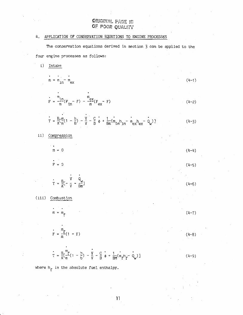
4. APPLICATION OF CONSERVATION EQUATIONS TO ENGINE PROCESSES

The conservation equations derived i n sect ion 3 can be applied t o the

four engine processes as follows:

i) Intake

i i ) Compression

( i i i ) Combustion

where h is the absolute f u e l enthalpy. f

( i v ) Exhaust

Note that the fuel fraction of the mass flow r a t e through the exhaust

port , F could be different from the cylinder fue l f ract ion, F, in reverse ex'

flow situations.

5. MODELLING OF ENGINE PROCESSFS

5.1 Gas Exchang2

A one-dimnsional quasi-steady compressible flow m d e l is used t o

calculate the mass flow r a t e s through the intake and the exhaust valves during

the gas exchange process. The manifolds a r e treated a s plenums with known

pressures. Furthermre, the temperature and average fquivalenqe r a t i o of the

intake charge (fresh a i r and ECFL at intake manifold conditions) and the

exhaust charge (mixture of a i r and ccmbustion products a t cylinder conditions)

a re known. When reverse flow into the intake manifold occurs, a rapid-mixing

mde l is used, i .e . perfect and instantaneous mixing between the back-flowing

charge and the intake charge is assumed.

A t each s tep of the gas exchange process, values for the valve open areas

and discharge coeff icients a r e obtained from tabulated data. Given the open

area, the discharge coeff icient , and the pressure r a t i o across a particular

valve, the mass flow r a t e across that valve is calculated from:

where

c = discharge coefficient d

A = valve open area

Po = stagnation pressure upstream of r e s t r i c t ion

p = s t a t i c pressure a t r e s t r i c t i on S

T = stagnation temperature upstream of r e s t r i c t i on 0

Y = r a t i o of specif ic heats

R = gas constant

When the kinet ic energy in the cylinder is negligible, the stagnation

pressure and temperature reduce to the s ta t i c pressure and temperature,

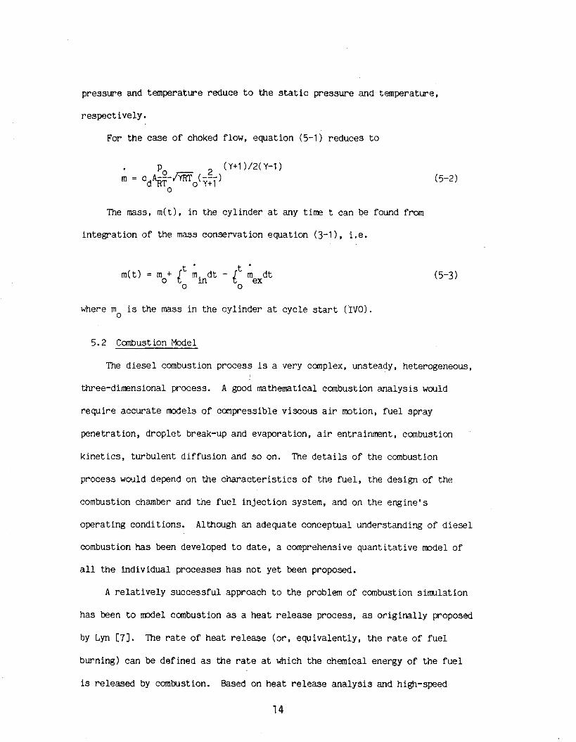
respectively . For the case of choked flow, equation (5-1) reduces to

The mass, m(t), in the cylinder a t any time t can be found from

integration of the mass conservation equation (3-1 ) , i.e.

where m is the mass in the cylinder a t cycle s t a r t ( I V O ) . 0

5.2 Combustion Model

The diesel combustion proces? is a very complex, unsteady, heterogeneous,

three-dimensional process. A good m thematical combust ion analysis wculd

require accurate models of compressible viscous a i r motion, fuel spray

penetration, droplet break-up and evaporation, a i r entrainment, combustion

kinetics, turbulent diffusion and so on. The details of the combustion

process would depend on the characteristics of the fuel, the design of the

combustion chamber and the fuel injection system, and on the engine1 s

operating conditions. Although an adequate conceptual understanding of diesel

combustion has been developed to date, a comprehensive quantitative mdel of

a l l the individual processes has not yet been proposed.

A relatively successful approach to the problem of combustion simulation

has been to mxlel ccmbustion as a heat release process, as originally proposed

by Lyn [7]. The rate of heat release (or, equivalently, the rate of fuel

burning) can be defined as the rate a t which the chemical energy of the fuel

is released by combustion. Based on heat release analysis and high-speed

photography, Lyn has provided an excellent description of the d i f fe ren t stages

of d iese l canbustion. These stages can be ident i f ied on the typical rate of

heat release diagram for a D I engine shown in Fig. 2 a s follows:

Ignition delay (ab) : The period between the dynamic injection point ( the

point a t which the injector needle starts t o l i f t ) and the ignition point ( the

s t a r t of posit ive heat re lease due t o cmbustion).

Pre-mixed or rapid combustion phase (bc 1 : In t h i s phase, combustion of the

fuel which has mixed with a i r t o within the flamabili ty l i m i t s during the

ignition delay period occurs rapidly i n a few crank angle degrees. This

r e su l t s in the high i n i t i a l r a t e of burning generally observed i n direct-

injection d iese l engines.

Mixing controlled combustion phase (cd): Once the fue l and air premixed

during the ignition delay have been consumed, the heat release r a t e (or

burning r a t e ) is controlled by the r a t e a t which mixture becomes available for

burning. The heat release r a t e may or may not reach a second (usually lower)

peak in t h i s phase; it decreases a s t h i s phase progresses.

Late combustion phase (de) : Heat release continues a t a low r a t e w e l l in to

the expansion stroke. Eventually, the burning r a t e asymptotically approaches

zero. The nature of combustion during t h i s phase is not well understood.

Possible processes a r e tha t a smll fract ion of the fue l may not yet have

burned, o r energy present i n soot and fuel-rich cmbustion products can still

be released, e tc . Given the somewhat a rb i t ra ry limits of t h i s phase,

combustion mdeld usually focus on the main heat re lease periods, i.e. the

pre-mixed and mixing controlled combust ion phases.

1 5

Based on h i s observations, Lyn C71 proposed a method of predict ing

burning r a t e s f r m the r a t e of f u e l in jec t ion. The f u e l in jec ted is divided

in to elements according t o the order i n which they en te r the combustion

chamber. These f u e l elements become "ready fo r burning1! according t o a

c e r t a i n law (with increasing burning time a s in jec t ion proceeds). Thus, a

"ready f o r burning" diagram can be obtained from the r a t e of in jec t ion

diagram. A t the ign i t ion point , which occurs a f t e r the lapse of the delay

period, the pa r t of the in jec ted f u e l which has been made "ready f o r burning"

is added on the t o t a l "ready f o r burning" diagram, causing the sharp peak i n

the burning r a t e diagram. Subsequent burning is e s s e n t i a l l y proportional t o

the r a t e of in jec t ion. Although t h i s method gives a reasonable f i t t o data

obtained over a wide range of speeds and loads, it requires fu r the r refinement

and c a l i b r a t i o n before it can be used i n canputer simulation work.

I t is necessary i n combustion modelling, in the context of computer

simulation t o predic t the performance of new engine concepts, t o describe the

apparent f u e l burning r a t e by a lgebraic expressions. The constants in these

expressions can be chosen su i t ab ly t o r e f l e c t the dependence of the ac tua l

f u e l burning r a t e on engine type and pa r t i cu la r operating conditions.

Shipinski e t a 1 C83 attempted t o cor re la te the apparent r a t e of f u e l

burning with the r a t e of f u e l in jec t ion by f i t t i n g a Wiebe function t o heat

r e l ease diagrams obtained from t e s t s on a high-speed swirl-type d i r e c t

in jec t ion engine. Although Shipinski obtained a reasonable agreement with h i s

engine da ta , the heat r e l ease shape defined by the Wiebe function alone has a

notable d i f ference f ran the two-part c h a r a c t e r i s t i c with the i n i t i a l spike

tha t is measured on mst engine types.

To overcome t h i s problem, Watson e t a 1 C91 proposed t h a t the apparent

f u e l burning r a t e could be expressed a s the sum of two components, one

r e l a t i n g t o pre-mixed and Ule o the r t o diffusion-controlled burning, i .e.

16

where m is the fue l burning r a t e with respect t o crank angle

and subscripts t , p, d denote t o t a l , pre-mixed and diffusion burning,

respectively.

In order t o quantify the proportion of the fue l burnt by e i ther

mechanism, a phase proportionality factor , 0, is introduced. This expresses

the cumulative fue l burnt by pre-mixed burning a s a f ract ion of the t o t a l fue l

injected, i .e.

Consequently, 3 non-dimnsional apparent fue l burning r a t e curve can be i

written a s

where M( T) = non-dimnsional burning r a t e dis t r ibut ion

and T = normalized crank position.

The phase proportionality factor , 5 , is considered t o be controlled by

the length of the ignition delay period (since the fue l that is prepared for

burning during t h i s period governs the pre-mixed burning phase), and the

overal l cylinder equivalence r a t i o , $ This can be expressed by a ove '

re la t ion of the fom

where I D = ignition delay (see Section 5.3).

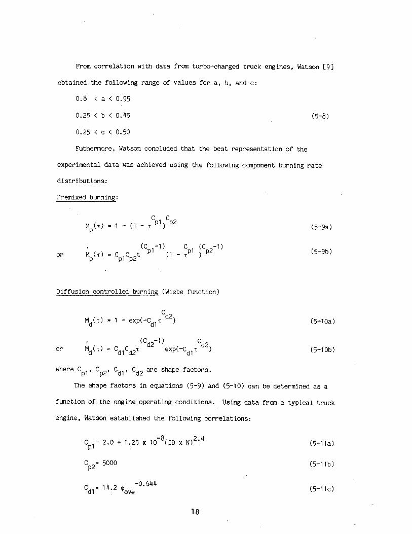
From c o r r e l a t i o n with d a t a f r a n turbo-charged t ruck engines, Watson [9]

obtained the fol lowing range of va lues f o r a , b, and c :

0.8 < a < 0.95

Futhermore, Watson concluded t h a t the b e s t r ep resen ta t ion o f the

experimental d a t a was achieved us ing the fol lowing canponent burning rate

d i s t r i b u t i o n s :

Premixed burning:

Diffusion con t ro l l ed burning (Wiebe func t ion )

where C C C d l , Cd2 are shape f a c t o r s . p l ' p2'

The shape f a c t o r s i n equat ions (5-9) and (5-1 0 ) can be determined as a

funct ion o f t h e engine opera t ing condi t ions . Using d a t a f r a n a t y p i c a l t ruck

engine, Watson e s t ab l i shed the fol lowing co r re l a t ions :

C = 1 4 . 2 $ -0.644

d 1 ove

where

ID = ignition delay (see Section 5.3)

N = enginespeed (RPM)

'ove = overal l cylinder equivalence ra t io .

Watson's correlat ion gives good agreemnt betveen experimntal and

predicted r e su l t s over the en t i r e range of engine operating conditions, and is

f lex ib le enough t o be applied t o various types of d iese l engines. Tnus, we

have followed Watson's approach t o describe the heat release prof i le for our

engine simulation. I f necessary, the constants (or the form) of correlat ions

(5-7) and (5-1 1) w i l l be modified t o f i t experimental data for our engine

design.

5.3 Igni t ion Delay Model

The ignition delay period i n a d iese l engine was defined i n section 5.2

a s the tire (or crank angle) interval between the start of inject ion and the

start of combustion. The start of inject ion is usually taken a s the tire when

the injector needle l i f t s off its sea t (determined from a needle l i f t

indicator). Tne start of combustion is more d i f f i c u l t t o determine. It is

&st ident i f ied from the change i n slope of the heat release rate which occurs

at ignition.

Both physical and chemical processes must take place before the injected

fue l can Ijurn. The physical processes are: the atomization of the l iquid

fue l jet; the vaporization of the fue l droplets; the mixing of fue l vapor with

a i r . The chemical processes a r e the precmbust ion reactions of the fue l , air,

residual gas mixture which lead to autoignition. These processes are affected

by engine design and operating variables, and fuel characteristics.

Ignition delay data from fundamental experiments in combustion bombs and

flow reactors have usually been correlated by equations of the form

I D = A p-n exp(E/RT) (5-12)

where I D = ignition delay [msl

E = apparent activation energy for the fuel autoignition process

R = universal gas constant

p = gas pressure Catml

T = gas temperature [K]

and A and n are constants dependent on the fuel and the injection and

air-flow characteristics. Representative values for A, n and E are given in

Table 1 . These correlations have usually been derived from tes t s i n uniform a i r

environments where the pressure and temperature only changed due to the

cooling effect of the fuel vaporization and fuel heating processes. However,

i n a diesel engine, pressure and temperature change considerably during the

delay period due to the compression resulting f'rcin piston mtion. .hother

problem is that the form of these simple correlations is not sufficiently

flexible to allow a l l the influencing fuel and engine parameters to be

included i n the ~a lcu la t ion of the ignition delay.

Hardenberg and Hase [I01 have developed an empirical formula for

predicting the ignition delay in D I engines as a function of fuel

characteristics, engine parameters and ambient conditions. Dent [ I 1 1 has

shown that this formula can give reasonable agreemnt with experimental data

over a wide range of engine conditions. However, the pressure and temperature

used in t h i s correlation a re identified a s the corresponding conditions at top

deal centre, estirrated using a polytropic m e 1 for the compression process.

It is f e l t tha t such a polytropic model is not appropriate in our s i m l a t i o n

context, where pressures and temperatures can be accurately predicted over the

duration of the ignition delay period. Therefore, we propose t o use a formula

similar t o Equation (5-1 21, with pressure and temperature taken a t the i r

arithmetic mean values during the delay period t o account for changing

condi t ions.

5.4 Heat Transfer

The heat transfer mechanisms in a d iese l engine include forced convection

( Q ) from the turbulent flow in the cylinder to the combustion chamber walls, C

and radiation (Q ) from the flame and the burning soot par t ic les . The t o t a l r

heat transfer r a t e ( Q ) is therefore given by W

+

The convective heat transfer a t the gas-to-cylinder wall interface w i l l

depend on the temperature gradient in the boundary layer a t the surface.

However, due t o the inherent d i f f i cu l t i e s i n calculating the boundary layers

i n a diesel engine, the convective heat transfer r a t e is usually expressed 2s

where

h = convective heat transfer coefficient

A = surface area

T = bulk mean gas temperature f3

T = l o c a l su r f ace temperature on cy l inde r wall, head, o r p i s ton , a s W

appropr ia te .

The problem is then t o dev i se a method t o c a l c u l a t e the convective hea t

t r a n s f e r c o e f f i c i e n t t h a t appears i n (5-1 4 ) . The approach usua l ly taken is t o

c a l c u l a t e h f r a n a Nusselt-Reynolds number c o r r e l a t i o n analagous t o t h a t used

f o r s teady tu rbu len t flow i n a p ipe [12-161, i .e .

where

Nu = hL/A : Nusselt number

Re = VL/v : Reynolds number

P r = pc / / A : Prandt l number P

L = a c h a r a c t e r i s t i c length

V = a c h a r a c t e r i s t i c v e l o c i t y

X = thermal conduct iv i ty

v = kinematic v i s c o s i t y

p = dynamic v i s c o s i t y

p = dens i ty

c = s p e c i f i c h e a t a t cons tant pressure P

and a , d , e are cons t an t s ad jus t ed t o f i t experimental data.

For tunate ly , t h e r e is l i t t l e v a r i a t i o n i n t h e Prandt l number f o r a i r and

combustion products , which is usua l ly c l o s e t o uni ty . Consequently, w e may

drop t h e P rand t l number dependence i n equation (5-15) with l i t t l e l o s s i n

accuracy, s o t h a t

Nu = a Re d (5-1 6 )

To c a l c u l a t e the convective h e a t t r a n s f e r c o e f f i c i e n t from c o r r e l a t i o n

2 2

(5-1 6 ) , instantaneous values for the character is t ic length and velocity

scales , and the gas transport properties (p, p , and A) a r e needed. Currently,

it is not possible t o predict these paramters and the i r spa t i a l and temporal

variation with any accuracy in an internal combustion engine. To overcome

t h i s d i f f icu l ty , representative values of the character is t ic length and

velocity scales , and the gas temperature, pressure, and equivalence r a t i o a t

which the gas properties a r e t o be evaluated a re chosen.

For our heat transfer model, the character is t ic length scale is taken t o

be the macroscale of turbulence, a s defined by equat ion (5-28) . (See

turbulent flow model). The character is t ic velocity V is postulated t o be an

effect ive velocity due t o contributions from the mean kinetic energy, the

turbulent kinet ic energy and piston motion, i.e.

where

U = mean flow velocity, defined by (5-20)

u f = turbulent intensity, defined by (5-21 )

V = instantaneous piston speed P

While t h i s expression for V is speculative, it is constructed in such a

way tha t increases i n any of the three component veloci t ies lead t o increases

i n the heat transfer r a t e , while a t the same tire er rors due t o overest imting

the contribution from any one component are minimized.

Many attempts have been reported t o determine the constants a and d,

e i ther by experirrjents or t r i a l and error. [I 2-1 61. Suggested values are

depending on intensi ty of change motion. The gas density and the transport

2 3

properties, p and A, that appear in correlation (5-1 6) are evaluated a t the

mean gas temperature, pressure, and equivalence ratio.

Radiative heat flux is significant in diesel engines. However, due to

the diff iculty of measuring instantaneous flame temperature and heat flux, it

is not easy t o quantify the contribution of radiation t o the overall heat

transferred. Estimtes of the relat ive importance of radiation have varied

between a few and 30 percent of total heat transfer, and vary according to

engine type. [13,14,17,181.

Annand [ I 31 has expressed the radiation term as

where

kr = empirical radiation constant

T = b u l k mean gas temperature g

T = local surface temperature on cylinder wall, head or piston, W

as appropriate

During the intake, compression and exhaust processes, when the radiative

heat flux would be zero, kr = 0. During combustion, Annand and Ma [ I 4 1

suggested that

kr = Cro

2 4 where o = Stephan-Boltzmann constant (56.7~10'~ kwlm K ) ,

and C is an adjustable constant with value3 in the range of 1.3 - 3.1, r

depending on the engine speed and load. The value of Cr, exceeding unity,

suggests that the actual radiation temperature is appreciably above the bulk

mean value.

Spatial variations i n heat transfer rates are accounted for by assigning

different surface temperatures to the cylinder walls, head, piston, etc.,

2 4

based on prac t ica l experience. I f these temperatures a r e t o be calculated, a

heat conduction M e 1 is required for the piston, valves, cylinder head, and

1 iner . The t o t a l instantaneous heat t ranfer r a t e w i l l be calculated fran the sum

of the convective terms (predicted by equation 5-1 4) plus the sum of the

radiat ive terms (predicted by equation 5-1 9 ) .

5.5 Turbulent Flow Model

The heat t ransfer model of the cycle simulation requires e s t i m t e s of the

charac te r i s t ic velocity and length scales. To e s t i m t e these scales i n a way

which incorporates the key physical mechanisms affect ing charge motion i n the

cylinder, a turbulent flow m d e l is used. This m d e l is a var ia t ion of the

models used by Manscuri C51 and Poulos C41 in previous engine s i m l a t i o n work.

The turbulence m d e l consis ts of a zero-dimensional energy cascade. Mean

flow kinet ic energy, K , is supplied t o the cylinder through the valves. Mean

kinet ic energy, K is converted t o turbulent kinet ic energy, k , through a

turbulent diss ipat ion process. Turbulent k ine t ic energy is converted t o heat

through viscous dissipation. When mass flows out of the cylinder, it ca r r i e s

with it both mean and turbulent k ine t ic energy. Figure 3 i l l u s t r a t e s the

energy cascade mdel .

A t any t ins3 during the cycle, the mean flow velocity, U , and the

turbulent intensi ty , u l , a r e found fran knowledge of the wan and turbulent

kinet ic energies, K and k , respectively. Thus, the following equations apply:

where the factor 3 in equation (5-21) comes f r m assuming that the sm11 scale

turbulence is isotropic (and accounting for a l l three orthogonal fluctuating

velocity components).

The time rate of change of the mean kinetic energy, K is given by

Similarly, the rate of change of the turbulent kinetic energy, k, is

where m = mass in the cylinder

m.= mass flow rate into the cylinder 1

m = mass flow rate out of the cylinder e

V . = jet velocity into the cylinder 1

P = rate of turbulent kinetic energy production

E = rate of turbulent kinetic energy dissipation per unit mass

A = ra te of turbulent kinetic energy amplification due to rapid

distortion

9. = characteristic size of large-scale eddies

In equations (5-22) and (5-,23), the production term P has to be defined

in terms of flow and geometrical parameters of the chamber. However, since

the above mdel does not predict spatially resolved flow parameters, P must be

estimated f r m mean flow quantities only.

Assuming tha t turbulence production in the engine cylinder is similar t o

turbulence product ion in a boundary layer over a f l a t plate [19], we can

express P a s

au ' P = 11 (--) t ay

(5-25)

2 where u = C k /(ME) is turbulent viscosity, t 11

and C = 0.09 is a universal constant. u

Again, a s the velocity f i e l d i n the cylinder is not known, the velocity

gradient ( aU/ay) is approximted a s

a u 2 u 2 (--I = c (-1 ay B L

(5-26)

. rere C is an adjustable constant and L is a gecmetric length scale. B

Using equations (5-251, (5-26 , ( 5-20) and (5-24) , we can express P a s

1 /2 3 3/2 KO 5 . P = 2 ( 5 ) C c (--I(

u B L 2 m (5-27)

Furthermore, the character is t ic s i ze of the large-scale eddies, L, and

the representative g e o ~ t r i c length scale, L w i l l be both identified with the

macroscale of turbulence, assumed t o be given by

2 2 = L = V/(TB 14) ( 5-28a

where V is the instantaneous volume of the combustion chamber and 3 is the

cylinder bore, subject t o the res t r ic t ion that

L 2 B/2 (5-28b )

Hence, equat ion can be re-written a s

During the co;inpression and the combustion processes, the turbulent

k i n e t i c energy decays due t o viscous diss ipat ion. On the o the r hand, a t the

same time the turbulent k i n e t i c energy is amplified due t o the rapid

d i s t o r t ion t h a t the cylinder charge undergoes with r i s i n g cylinder pressures.

Consequently, an amplif ication term, A, was added t o equation (5-23) t o

account f o r t h i s e f f e c t . The amplif ication term w i l l be l a rge r during

combustion when the unburned gas is assumed t o be compressed by the flame a t a

s u f f i c i e n t l y high r a t e . However, i n the d i e s e l engine context (high

cmpress ion r a t i o s ) , i t is proposed t o keep the amplif ication term during

canpresson, too.

Using equation (5-21), the r a t e of turbulence amplif ication due t o rapid

d i s t o r t i o n can be expressed as

where the r a t e of change of the turbulent in tens i ty d u f / d t can be estimated

assuming t h a t conservation of mass and angular momentum can be applied t o the

large s c a l e eddies during the rapid d i s t o r t i o n period.

Under these assumptions, conservation of m a s s fo r a s ing le eddy of volume

V requires tha t L

where p is the mean gas densi ty and subscr ip t o r e f e r s t o the condit ions a t

the s t a r t of cmpression. Then, s ince

where L is the macroscale of turbulence, we can re-write (5-31) as

2 8

Conservation of eddy angular momentum requires that

U L = U L W wO 0

mere U is the character is t ic velocity due t o eddy vort ic i ty . W

Combining (5-33) and (5-34) with the assumption that

the following re la t ion is obtained for the evolution of the turbulent

intensity during the rapid canpression period

Differentiating both sides of equation (5-36) and re-arranging we get

du' - - u1 -- Q - dt 3p d t

Hence, combining equations (5-30) and (5-371, the r a t e of turbulence

amplification is given by

o r , introducing (5-21 1,

with p given from equation (3-15).

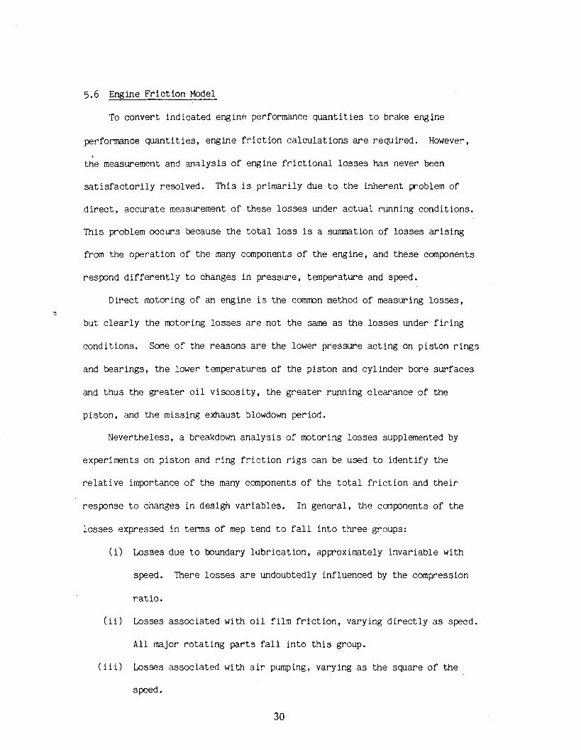
5.6 Engine Fr ic t ion Model

To convert indicated engine performance quan t i t i e s t o brake engine

performance quan t i t i e s , engine f r i c t i o n ca lcu la t ions a r e required. However,

the measurement and ana lys i s of engine f r i c t i o n a l losses has never been

s a t i s f a c t o r i l y resolved. This is primarily due t o the inherent problem of

d i r e c t , accurate measurement of these losses under a c t u a l running conditions.

This problem occurs because the t o t a l l o s s is a s u m t i o n of losses a r i s i n g

from the operation of the many components of the engine, and these components

respond d i f f e r e n t l y t o changes i n pressure, temperature and speed.

Direct motoring of an engine is the commn method of measuring losses ,

but c l e a r l y the m t o r i n g losses a r e not the same a s the losses under f i r i n g

condit ions. Sane of the reasons a r e the lower pressure ac t ing on pis ton r i n g s

and bearings, the lower temperatures of the p is ton and cylinder bore surfaces

and thus the greater o i l v i scos i ty , the g rea te r running clearance of the

p is ton, and the missing exhaust blowdown period.

Nevertheless, a breakdown ana lys i s of motoring losses supplemented by

experiments on pis ton and r ing f r i c t i o n r i g s can be used t o ident i fy the

r e l a t i v e importance of the many components of the t o t a l f r i c t i o n and t h e i r

response t o changes i n desigh var iables . In general , the ccmponents of the

losses expressed i n terms of mep tend t o f a l l in to th ree groups:

( i ) Losses due t o boundary lubr ica t ion , approximtely invar iable with

speed. There losses a r e undoubtedly influenced by the compression

r a t i o .

( i i ) Losses associated with o i l f i lm f r i c t i o n , varying d i r e c t l y a s speed.

A l l major r o t a t i n g p a r t s f a l l in to t h i s group.

( i i i ) Losses associated with a i r pumping, varying a s the square of the

speed.

3 0

Therefore, the mtoring losses can be expressed i n the form

F = A + B N + C & ( 5-39 )

where F a r e the losses in mep, N is engine speed, and A, B and C a r e

constants.

Millington and Hartles [201 have measured motoring losses on a large

variety of automotive diesel engines during the course of development of

prototype engines. Their work suggests a readjustment of equation (5-39)

coupled with sui table selection of the constants a s follows:

where F = motoring losses, ps i mep

A = compression r a t i o minus 4 for a D I d iesel

N = engine speed, rpm

V = mean piston speed, fpm

Equation (5--40 ) repyesents a sound empirical correlation of the motoring ' , L :

loss data obtained from diese l engines. Therefore, it w i l l be used t o obtain

brake quantit ies from the indicated quantit ies computed in the engine

simulation.

6. BASIC ASSUMPTIONS O F OTHER COMPONENT M I D E L S

The configuration of the turbocharged, turbocompounded , Diesel system was

zhown in Fig. 1 . I t consis ts of a ccmpressor, intercooler, intake manifold,

intake ports t o the engine, multicylinder engine, exhaust ports, exhaust

manifold, wastegate, turbocharger turbine, compounded turbine and associated

ducting. The following simplifying assumptions were made in order t o develop

mde l s of the components required in addition t o the diesel engine t o canplete

the overall system.

1 . The intake a i r is a t atmspheric conditions:

'1 = Patm and TI - - Tatm

2. The compressor, turbine and power turbine a re adiabatic; i .e. there is no

heat t ransfer from these conponents t o the environment.

3. There a re no mass t ransfers except along the routes indicated; i.e. no

loss o r leakage from the system.

4. Intake a i r and exhaust gas can be modelled a s ideal gases.

5. The connecting pipes to and from the manifolds can be included as parts of

their respective manifolds, for modelling purposes.

6. There is perfect and instantaneous mixing of a l l mass flows that enter

each -i%nifold with the gases in the manifold, thus there is no variation

in properties within a manifold a t any instant of t i r e , md a l l flows

leaving a manifold have the properties of the manifold contents.

7 . The wastegate bleeds off a f ract ion of the exhaust gas stream ( r i ~ 1, such W

that the flow bypasses the turbocharger turbine b u t not the pwer turbine.

8. The wastegate valve behaves a s a t h ro t t l e valve of variable effective

throat area. The s ize of the opening can be governed by the intake

manifold pressure, p 5'

9. The EGR flow is e i ther spec i f ied a s a f ract ion of the intake flow, or the

EGR valve is modelled a s a th ro t t l e valve of fixed effect ive throat area.

10. The flaws through the wastegate and EGR valves a r e subsonic and adiabatic,

and the throat pressures a r e eq~zal t o the downstream pressures.

11. The two exhaust gas streams, through and by-passing the turbine, (5 and t

i% ) reunite with no lo s s of thermal energy or pressme. W

12. The inside wall temperature of a l l components i n the system a r e known.

13. There are pressure drops between the following:

compressor discharge and intercooler in le t (p & p ) 2 3

intercooler i n l e t and intake manifold (p & p ) 3 5

exhaust manifold and turbine in l e t (p & p8) 7

turbine discharge and power turbine in l e t (p & p ) 9 10

power turbine discharge and atmsphere (p, & ~ a t m )

14 . Wastegate upstream pressure equals turbine in le t pressure.

15. Wastegate downstream pressure equals turbine discharge pressure.

16. Turbine and ccmpressor speeds a re equal.

17. The turbocharger (turbine, compressor and shaf t ) has fixed values of

rotat ional i ne r t i a and damping, r e l a t i ve t o its housing (J and B,

respectively) . 18. The power turbine shaft is connected t o the engine crankshaft via a

specified gear r a t i o transmission, thus the power turbine speed is always

determined d i rec t ly from the engine speed.

7. MODELLING OF SYSTEM COMPONENTS

7.1 State Variables

The turbocharged diesel engine system described i n Sec. 6 can be modelled

mathemtically by a set of simultaneous, non-linear differential equations

involving a minimum set of dependent variables. These variables, called the

s ta te variables, are sufficient to describe canpletely the system a t any point

in time. Although their number is fixed by the system, there are many choices

of s t a te variables, some mre convenient than others. The mass, temperature,

absolute pressure and fuel fraction states of each manifold and the

turbocharger speed were chosen as the nine s ta te variables of t h i s system.

Crank-angle was chosen as the independent variable, rather than t i m e . Since

we are studying constant speed performance, time and crank-angle are directly

proportional. A l l mass flow rates ( m ) i n the following analysis refer t o mass

flow per unit crank angle.

7.2 Derivation of Differential Equations

7.2.1 Manifolds

The four s ta te equations for each manifold are derived from four

interdependent relations for the manifold control volume:

1 . conservation of total mass

2. conservation of fuel mass

3. conservation of energy ( f i r s t law of thermodynamics)

4 . ideal gas law

The general manifold control volume model is shown in Fig. 4. The total

mass and fuel fraction s ta te equations for the mnifold come directly from the

continuity relations derived earl ier (Equations (3-1 ) and (3-5),

respectively) :

where the subscript m re fe rs t o the manifold control volume, and the subscript

j r e f e r s to the j-th mass flow that enters or leaves the control volume.

For the intake manifold, the mass flows entering and leaving the manifold

include:

i ) compressor mass flow (m in Fig. 1 ) (entering) which is found from the C

compressor map

ii) engine intake mass flow (m in Fig. 1 ) (leaving) which is found in

from the engine model .

iii) EGR mss flow ( mEm in Fig. 1 j (entering) which is found frcm the

EGR valve equations

For the exhaust manifold, the mass flows entering and leaving the

manifold include:

i ) t k b i n e mass flow (rn i n Fig.1) (leaving) which is found frcm the t

turbine map

ii) engine exhaust mass flow (m in Fig. 1 ) (entering) which is found ex

from the engine model

iii) EGR m s s flow (- mEQ( in Fig. 1 ) (leaving) which has the opposite

sign t o intake EGR flow)

BW1GlNAL PAGE 19 09: BOOR QUALITY

i v ) wastegate mass flow (m i n Fig. 1 ) ( l eav ing ) which is found from t h e W

wastegate valve model

The s t a t e equat ion f o r temperature is der ived from t h e gene ra l temperature

s t a t e equat ion (3-26) appl ied t o t h e m n i f o l d c o n t r o l volume.

where A , B, and C a r e def ined i n (3-27), (3-24), (3-28) and are ca l cu l a t ed by

the thermodynamic proper ty subrout ine ,

Q = heat t r a n s f e r rate t o t h e manifold walls

and d4/dt is r e l a t e d t o dF/dt and F by (3-8).

The state equat ion f o r p re s su re is der ived from the gene ra l pressure

s t a t e equat ion app l i ed t o t h e manifold c o n t r o l volume (Eq. 3-21):

The mass, f u e l f r a c t i o n and temperature d e r i v a t i v e s a r e ca l cu l a t ed i n

equat ions (7 - I ) , (7-2) , and (7-3); t h e equivalence r a t i o d e r i v a t i v e , d$ /d t , is

r e l a t e d t o the r u e 1 f r a c t i o n d e r i v a t i v e by Eq. (3-85 ; and the dens i ty

d e r i v a t i v e s a r e c a l c u l a t e d by t h e thermdynamic property subrout ine .

7.2.2 Turbocharger

The state equat ion descr ib ing the turbocharger is der ived from t h e

conserva t ion of energy r e l a t i o n .

d-(E ) = W d t t / c compressor + ' turbine

d where E ) = J w d W + B w

2 d t t/c d t

E t / c = t o t a l mechanical energy o f turbocharger r o t o r

QRIG1NAL P&GE IS OF POOR QUAL9TT

J = rotat ional i ne r t i a of turbocharger

B = rotat ional damping of turbocharger

w = angular velocity

'turb ine = mt(h8- hg)

Solving for dw/dt gives:

Tne enthalpy changes across the compressor and turbine a r e calculated using

the compressible flow relat ions.

The complete s t a t e equation for turbocharger is found by combining equations

(7-91, (7-lo), and (7-11).

7.3 Wastegate and EGR Valve Models

The wastegate and exhaust gas recirculation (EGR) valves a r e modelled a s

adiabatic t h ro t t l e valves of known effect ive throat area (which is the product

of actual cross-sectional area and a discharge coefficient. The mass flow

ra t e s through the valves a r e calculated using (5-1) and (5-2).

To determine the EGR flow ra t e , e i ther the percentage of the ergine in l e t

flow which is EGR is specified, or the EGR valve openiw is treated a s a fixed

effective-area or i f ice .

The wastegate valve opening area varies between zero and a fixed maxirrmm

value, (CDA),,x, and is determined by an actuator linked to a pressure sensor.

The sensor measures the gage pressure of the intake manifold. A t present, a

simple actuation model has been adopted which gives a continuous closed-form

relation between effective valve throat area and intake manifold pressure.

This mdel can be replaced when the actual actuator characteristics are

available.

7.4 Intercooler Model

The intercooler, which is situated between the compressor discharge and

intake manifold, serves to increase the density of the charge a i r by lowering

its temperature. The intercooler is modelled as a heat exchanger of fixed

area, heat-tranfer coefficient and cooling flow rate. The change in charge

a i r temperature is determined from the non-dimnsional heat exchanger

ef fect iveness, E.

where h r e f e r s t o t h e c h a r g e a i r f l o w ( h o t )

c refers to the coolant flow (cold)

1 and 2 refer t o inlet and exi t conditions respectively

Thl = compressor discharge temperature, T2

Th2 = intercooler discharge temperature,

Tcl = coolant inlet temperature (assumed to be fixed)

Heat exchanger effectiveness is either known as a design parameter or can

be derived from graphical correlations that are available for the various

typical heat exchanger configurations. From the l a t t e r E can be determined as

a function of capacity r a t e r a t i o , C /C min mx ' and number of heat transfer

un i t s , NA, where

'min = the lesser of the two values of mc (assumed t o belong t o the

P

charge a i r flow),

Cmx = the greater of the two values of mc (assumed t o belong t o the P

coolant flow and t o be fixed) ,

A = heat exchange surface area (fixed)

U = heat transfer coefficient based on A

Fig. 5 shows a graphical correlation for a cross-flow heat-exchanger with

unmixed flows, with various r a t i o s of C /C Currently the assumption is min m x '

being made tha t Cmx is much larger than C . With t h i s assumption the mm '

expression for effectiveness reduces t o the following simple form:

7.5 Manifold Heat Transfer

With the incorporation of an intercooler, heat transfer f r m the intake

manifold t o the environment becomes smll enough t o be rieglected. Heat I

transfer from the exhaust manifold, however, cannot be neglected. Heat

t rv l s f e r from the gas i n the exhaust manifold t o the e n v i r o m n t involves a

combinat ion of forced convective' heat transfer from the gas t o the inside

walls, conduction from the inside walls t o the outside walls and t o the water

jacket, and natural (and probably forced) convection f r m the outer surfaces

t o the environment.

I t is c lear ly a complicated process t o determine f u l l y the heat transfer

from inside gas t o outside a i r , involving mny detailed assumptions about

engine geometry and environmental flow conditions. To simplify t h i s t a s k in

39

the current generation simulation program we w i l l deal only with the modelling

of the heat transfer from manifold gas to interior walls, which necessitates

that a value for the wall temperature be assumd.

The heat transfer coefficient is derived from an e x p e r i ~ n t a l correlation

that relates Nusselt, Reynolds and Prandtl numbers for fully-developed

turbulent flow in circular tubes with large temperature gradients (Eq. 7-14).

where D = exhaust manifold diameter

V = average velocity of gas

The gas properties are:

k = thermal conductivity

p = absolute viscosity

p = density

c = specific heat a t constant pressure P

Subscripts are:

b: refers to properties a t T b *

f : refers to properties a t T f '

Temperatures are:

T = bulk (avers,?) temperature b

Tw = wall temperature

T = "film" temperature, f

7.6 Pressure L a s e s

Pressure l o s s terms have been included a t f ive locations in the overal l

system nmdel. These are:

between compressor discharge and intercooler i n l e t ,

across intercooler,

between exhaust m i f o l d and turbine i n l e t ,

between twb ine out le t and power turbine in l e t

between power turbine out le t and atmsphere.

Each of these pressure drops is calculated using the corresponding f r i c t i on

factors and f r i c t i on coeff icients for the geometry of each passage.

For straight-sect ions:

*ere L = length of passage

D = diameter of passage

p = bulk density

V = average velocity

f = f r i c t i on factor , which is correlated by (7-17) for the surface

roughness and range of Reynolds numbers t o be encountered.

Note that

with Re= pVD/p

For bends, enlargements, contractions, etc:

where K = f r i c t i on coefficient for a part icular passage geometry. Values f

of K for typical geometries a re c o m n l y available. f

8. THERM3DYNAMIC PROPEKT IES

Our themdynamic model assumes that the various control volumes contain

mixtures of a i r and canbustion products throughout the total engine system.

By utilizing the concept of the instantaneous average equivalence ra t io

defined in Section 3.1, the contents of any control volume can be represented

as one continuous medium. Furthermore, assuming ideal gas behavior and

thermdynamic equilibrium, the instantaneous gas properties can be determined

fran a knowledge of pressure, temperature and average equivalence rat io in the

control volume.

When the temperature of the cylinder contents is below 1000 K, they are

treated as a homogeneous mixture of non-reacting ideal gases, their properties

being calculated using the procedure outlined below [211:

The hydrocarbon-air canbustion reaction is written as:

c @ C H Y + 0 + O N + x CO + x2H20 + x CO + x4H2 + x 0 + +N 1 3 5 2 (8-1

where JI = the molar N:O rat io of the products,

y = the mlar H:C ra t io of the fuel,

@ = the average equivalence rat io,

xi = moles of species i per mole of 0 reactant 2

and E = 4/(4+y) ( 8-2

The quantities x. are determined by using the following assumptions: 1

a) for lean mixtures ( 4 S 1) H2 can be neglected.

b) for rich mixtures ( 4 > 1 ) O2 can be neglected.

c ) for rich mixtures, the gas water reaction

C02 + H2 + C02 + H20

is in equilibrium with equilibrium constant K(T).

The solution for the x. is shown in Table 11, where C is obtained by 1

solving equation (8-3) for its positive root.

The value of K(T) is obtained by curve f i t t i n g JANAF table data over the

temperature range 400 t o 3200 K and is given by

In(K(T)) = 2.743 - 1.761 /t - 1.61 1 / t 2 + .2803/t 3 ( 8-4

where t = T/1000, and T is the temperature i n Kelvins.

I f the grams of products per mole of 0 reactant is expressed a s 2

M = ( 8 ~ + 4 ) @ + 32 + 281) ( 8-5 1

the specif ic enthalpy h and the specif ic heats a t constant pressure and

constant composition, c and c respectively, can be expressed by the P $

following relationships :

The coeff icients a . a r e obtained by curve f i t t i n g JANAF table data t o the lj

above functional form. The values of a a r e given in Table 111. The i j

resultant c is in cal/g-K, while h and c a r e i n kcal/g. P $

Since the cylinder contents a r e being t reated a s a mixture of non-

reacting ideal gases, the density of the mixture is given by

where

Ro = the universal gas constant (1.9869 cal/mle-K)

and M, the average molecular weight of the mixture, is given by

M/((1 - € I $ + 1 + qJ) $ 5 1

and

Then, the part ial derivatives of the density wi th respect to

temperature, pressure, and equivalence ra t io are given by

'then the temperature of the cylinder contents is above 1000 K , their

properties are calculated with allowance for chemical dissociation, according

to the calculation method described i n C221. This is an approxirmte method

based on curve f i t t ing data obtained from detailed thermchmical calculations

[23] t o a functional form obtained f r m concentrations within the burned gases

are not calculated, the bulk thermodynamic properties needed for cycle

analysis are accurately determined.

9. TRANSPORT PROPERTIES

The heat t ransfer correlat ions r e l a t e the heat t ransfer coeff ic ient t o

the Reynolds and Prandtl numbers and the t h e r m l conductivity. The

calculation of the heat t ransfer r a t e s w i l l therefore require values for the

viscosi ty and the Praadtl number (from which the t he rml conductivity can be

obtained). We have used the approximte correlat ions for the viscosity and

the Prandtl number of hydrocarbon-air canbustion products developed by

Mansouri and Heywood C24 I.

The NASA equilibrium program C231 was used t o compute the viscosity of

hydrocarbon-air canbust ion products as a function of temperature, T,

equivalence r a t i o , +, and pressure p. It w x i shown that the v i s o s i t y of the

canbustion products was s a t i s f ac to r i l y correlated by a power-law based on a i r

viscosity data , corrected for the e f fec t of equivalence r a t i o , i .e . ,

-7 0.7/(1 p Ckg/msl = 3.3~10 T + 0.027$) prod

(9-1

for 500 K 5 T I4000 K

0 6 4 5 4

Note that the viscosity of the combustion products is independent of the

pressure.

The equilibrium Prandtl number of hydrocarbon-air combust ion products was

a l so calculated over the above ranges of temperature, pressure, and

equivalence r a t i o . Using a second order polynomial of Y t o curve f i t the

above data, it was shown that the following correlation for lean ( @ < 1)

mixtures predicted values in good agreemnt (within 5%) with the data, i.e.,

P r = 0.05 + 4 . 2 ( ~ - 1) - 6 . 7 ( ~ - 1 ) 2

fo r 500 K I T I 4000 K

and $ 5 1

For r ich mixtures (41 > I ) , a reasonable f i t ( l e s s than 10% er ror ) t o the

equilibrium Prandtl number values calculated with the NASA program was found

to be the following:

2 2 P r = C0.05 + 4.2(Y - 1 ) - 6.7(Y - 1) 3/11 + 0 . 0 1 5 ~ 1 0 - ~ ( ~ ~ ) 1

for 2000 K I T I 3500 K (9-2b

and 1 < $ 5 4

1 0. ITERATION PROCEDLTRE

1 0.1 Basic Method of Solution

When the individual submdels of the t o t a l engine system a r e brought

together t o form a complete mdel , the r e su l t is a s e t of simultaneous

f irst-order ordinary d i f ferential-equat ions. To perf om predictive

calculations with the cycle simulation, these equations must be integ-ated

simultaneously over the f u l l o p r a t i n g cycle. Note, however, that some of the

governing equations l i ke the mass flow r a t e through the intake or the exhaust

valve and the non-dimensional fue l burning r a t e apply only during parts of the

cycle.

Integration of the governing equations is performed numerically using a

standardized code developed by Shampine and Gordon [27]. The optimal

integration time s tep is calculated automatically in the routine so a s t o

maximize efficiency. Detailed documentation of the i n t e r a t i o n routine is

provided in the l i s t i n g of the code.

10.2 Crank Angle By Crank Angle Integration

The engine mdel calculates the s t a t e variables in one master cylinder of

a mult i-cylinder engine, while the manifold and other component models have

inherent multi-cylinder capability. The interact ion between the master

cylinder model and the other components takes place in the manifolds. To

simulate the e f fec t of additional cylinders on the manifold conditions and

hence on the en t i r e s y s t m behavior, the conditions i n the other cylinders a r e

assumed t o vary a s echoes of the f i r s t cylinder, shif ted by the appropriate

phase lags. The intake and exhaust mass flow profi les calculated by the

engine m d e l for the master cylinder a r e used t o represent the profi les fc r

the other cylinders. These profi les a r e u@ated a f t e r the completion of each

engine cycle for use in the next i terat ion.

4 7

A flow c h a r t showing t h e o v e r a l l s t r u c t u r e of t h e eng ine c y c l e

s i m u l a t i o n i s shown i n F igure 6. A f t e r t h e i n i t i a l i z a t i o n of t h e s t a t e

v a r i a b l e s , t h e s i m u l a t i o n proceeds w i t h t h e s imul taneous i n t e g r a t i o n of t h e

s t a t e e q u a t i o n s f o r t h e mani fo lds , t h e e n g i n e and t h e tu rbocharger . The

main program de te rmines which s e t s of e q u a t i o n s t n e i n t e g r a t o r w i l l work

wi th , and c a l c u l a t e s and p r i n t s o u r r e s u l t s a s t h e c y c l e proceeds . Four

secondary r o u t i n e s cor respond ing t o t h e i n t a k e , compressor , combustion, and

exhaus t p r o c e s s e s a r e c a l l e d i n t u r n by t h e i n t e g r a t i o n r o u t i n e t o supply i t

w i t h t h e d e r i v a t i v e s of t h e v a r i a b l e s which i t must i n t e g r a t e . A t h i r d

l e v e l of u t i l i t y r o u t i n e s , such a s t h e o t h e r component s t a t e e q u a t i o n s ,

thermodynamic and t r a n s p o r t p r o p e r t y r o u t i n e s , t a b l e s of v a l v e f low a r e a s

and d i s c h a r g e c o e f f i c i e n t s , i s c a l l e d by t h e second l e v e l r o u t i n e s t o h e l p

i n the e v a l u a t i o n of t h e n e c e s s a r y d e r i v a t i v e s a t each s t e p .

Approximate e s t i m a t e s o f a l l s t a t e v a r i a b l e s a t convergence a r e

assumed. In g e n e r a l , more than one i t e r a t i o n i s r e q u i r e d t o model an eng ine

o p e r a t i o n under s t e a d y c o n d i t i o n s . The i n t e g r a t i o n c o n t i n u e s u n t i l t h e

sys tem reaches a q u a s i - s t e a d y s t a t e , which i s d e f i n e d a s t h e s t a t e i n which

t h e v a l u e of each s t a t e v a r i a b l e a t a p a r t i c u l a r crank-angle i s t h e same ( t o

w i t h i n a s p e c i f i e d i n t e r v a l ) a s i t was a t t h a t crank-angle i n t h e p rev ious

e n g i n e c y c l e . Thus, a t quas i - s t eady s t a t e a s e t of r e p e a t i n g p a t t e r n s of

v a r i a t i o n , one f o r each s t a t e i n t h e sys tem and each w i t h a p e r i o d of one

e n g i n e r e v o l u t i o n , i s ach ieved .

1 1 . PROGRAM INPUTS AND OUTPUTS

11 .I Inputs

To operate the simulation, a set of input parameters must be specified.

These include f ixed system dirrensions, i n i t i a l values of state var iables and

computing tolerances. They a r e l i s t e d and b r i e f l y described below.

1 1 . l . 1 Engine operating condi t ions

i. f u e l type

ii. mss of f u e l in jected per cycle

iii. in jec t ion timing

iv. engine speed (rpm)

v. constants i n the ign i t ion delay cor re la t ion

vi . nominal burning duration

v i i . constants re la ted t o the burning r a t e d i s t r ibu t ions

1 1 . I .2 System d imns ions and design parameters

a. Engine paramters

i. number of cyl inders

i i. cylinder bore and s t roke

iii. clearance v o l m

iv. connecting rod length

v. valve timings (crank angles at which the intake and exhaust

valves open and close)

vi . tabulated values f o r the valve open a reas and discharge

coef f i c ien t s

b . Other component dimens ions

i. manifold dimnsions

ii. connecting passage dirrensions

iii. EGR and wastegate valve dimensions

iv. wastegate ac tuator c h a r a c t e r i s t i c s

c. In tercooler c h a r a c t e r i s t i c s

i. coolant flow hea t capacity

ii. heat exchange surface a rea

iii. heat exchanger hea t t r a n s f e r coe f f i c i en t

d. Turbomachinery parameters

i. turbocharger r o t a t i o n a l i n e r t i a

i i . turbocharger r o t a t i o n a l damping

iii. power turbine gear r a t i o

iv. power turbine transmission eff ic iency

v. compressor, turbine and power turbine maps

(see Sec. 11.2 - Turbocharger and power turbine maps)

11 .l. 3 Heat t r a n s f e r and turbulent flow parameters

a. constants f o r the Nusselt-Reynolds number cor re la t ion

b. the temperatures of the p is ton, cyl inder head, cyl inder walls and

manifold wal ls

c. the turbulent d i s s ipa t ion constant

1 1 .l. 4 Engine f r i c t i o n parameters

Empirical constants associated with the ca lcula t ion of f r i c t i o n losses

11.1.5 I n i t i a l condit ions

a. intake manifold pressure and temperature

b. exhaust manifold pressure and temperature

c . turbocharger speed

11.1.6 Ambient conditions

a . intake temperature

b. intake pressure

c . f i n a l exhaust pressure

11 . l . 7 Computational paramters

a . convergence mrgins for each s t a t e variable

b. error tolerances for i n t e p a t i o n of the d i f fe ren t ia l equations

c. other paramters used in the integration alwri thm

(For a detai led description of these parameters, see the engine

simulation code. )

1 1 .2 Turbocharger and Power Turbine Maps

Maps give the interrelationships amng mss flow r a t e , efficiency,

pressure r a t i o and rotor speed for each of the three turbomchinery

components: turbocharger compressor and turbine, and power turbine. The maps

a r e put into the simulat ion in tabular form and must therefore be reduced to

tabular form i f i n i t i a l l y in graphical form. The tables a r e interpolated

during the simulation t o find the necessary informtion. The map variables of

mss flow r a t e and rotor speed a r e corrected by factors re la t ing actual i n l e t

conditions t o standard conditions. The speed correction factor involves

i n l e t temperature, and the mass flow r a t e correction factor involves i n l e t

temperature and pressure.

The compressor map variables a r e 7 ) m 2 ) p2/p1 3) nc and 4) w. c ,

The mass flow r a t e is normlized according t o p and T The rotor speed is 8 8'

normlized according t o T 8'

The turbine map variables a r e 1) mt, 2 ) p$p9. 3) " and 4) o.

5 1,

\ The mass flow rate is normalized according t o p and T The rotor speed is 8 8'

normalized according t o T8.

Thepower turbinemapvariablesare 1 ) 1 2)p10/p11, 3) "t, 4 ) upt. pt '

Mass flow ra te is normlized according to p and TlO. The shaft speed, which 10

is directly determined from the engine speed and the specified gear rat io, is

normalized according to TlO.

11.3 Outputs

Four types of outputs are generated by the cycle simulation:

11.3.1 Input echo

A l i s t ing of a l l the input parameters, including some quantities derived

directly from the given inputs (e.g. engine displacemnt and compression

rat io)

11.3.2 Major crank-angle by crank angle results

A t specified crank-angle intervals, the values of the following s ta te

variables are returned:

a. cylinder pressure, temperature, and average equivalence ra t io

b. intake manifold pressure, temperature and average equivalence ra t io

c . exhaust manifold pressure, temperature and average equivalence rat io

d. turbocharger speed

In addition, the following other quantities are reported a t the same

intervals:

a. engine to ta l heat transfer rate

b. heat transfer rates to different surfaces of interest

c . engine work done

d. turbulent flow model results (such as mean flow velocity, turbulent

d. turbulent flow m d e l r e su l t s (such as mean flow velocity, twbulent

intensity, mcroscale of turbulence )

e. a code which monitors the performance of the integration routine

Integrating through the different processes for the master cylinder, the

following quantit ies a r e reported during the corresponding process:

a . Intake

i. mass flows through each valve

ii. mass fract ion of fresh charge (air) in the cylinder

b. Combustion

i. a non-dimnsional fue l burning r a t e

ii. fue l burnt a s a function of t o t a l fue l injected

c. Exhaust

i. mass flow r a t e and velocity through exhaust valve

11.3.3 Integrated resu l t s and cycle performance

After cmplet ion of an engine cycle, a s m r y of r e su l t s obtained by

integrating some of the governing equations over the cycle is given.

Integrated r e su l t s include the following:

a. volumetric and thermal eff ic iencies

b. gross indicated, pumping and f r i c t i on man effect ive pressures

c . t o t a l heat loss

d. ignition delay period

e. estimated mean exhaust temperature

f . mass in cylinder a t IVO and a t IVC

g. mass of a i r inducted per cycle

h. t o t a l heat and work transferred during each process

i. r e su l t s of an overal l energy balance

1 1 .3 .4 Sub-&el results

After the overall cycle results are l i s ted, detailed results for the main

sub-mdels of the cycle simulation are given a t specified crank angle

intervals. These quantities include the following :

a. total engine intake and exhaust mass flow rates

b. compressor, turbocharger turbine and power turbine mass flow rates,

pressure rat ios and efficiencies

c. wastegate (turbocharger turbine bypass) and ECR mass flow rates

d. power turbine work transfer

e. pressures and temperatures a t various system locations

f . intake and exhaust manifold heat transfer rates

g. intercooler effectiveness

12. REFERENCES

1 . Katz, N. R. and Lenoe, E.M. , "Ceramics for Diesel Engines : Preliminary Results of a Technology Asse~smen t ,~~ Progress :Report DOE/AMMRC LAG DE-AE 101 -77 CS51017, 1981 .

2. Kamo, R. and Bryzik, FJ. , "Adiabatic Turbocompound Engine Performance Predict ions ," SAE Paper 780068, 1 978.

3. Kamo , R. and Bryzik, W. , "Cumins-TARADCOM Adiabat LC T~rbocmpund Engine Program," SAE paper 81 0070, 1981.

4. Pculos, S.G. and Heywood, J.B., "The Effect of Chavber Gemetry on Spark- Ignition Engine Combu~tion,~ SAE paper 830334, 1983.

5. Mansour i , S. H. , Heywood, J. B. and Radhakrishnan, K. , "Divided-Chamber Diesel Engines, Part 1 : A Cycle-Simulation which Predicts Performance and Emissions," SAE Paper 820273, 1982.

6. iJatson, N. and Janota, M.S., Turbocharging the Internal Ccmbustion Engine, John Wiley & Sons, New York, 1982.

7. Lyn, W.T., "Study of Burning Rate and Nature of Combustion in Diesel Engine, " I X Symposium ( International) on Cmbust ion, Proceedings, pp. 1069-1082, The Ccmbustion Ins t i t u t e , 1962.

8. Shipinski, J . , Uyehara, O.A. and Myers, P.S., "Experimental Correlat im Between Rate-of-Inj ect ion and Rate-of-Heat-Release in a Diesel Engine, ASME Paper 68-DGP-11 , 1968.

9. Watson, N. , P i l ley, A.D. and Marzouk, M . , !'A Ccmbustion Correlation for Diesel Engine Simulation, " SAE Paper 800029, 1 980.

10. Hardenberg, H.O. and Hase, F.W., "An Empirical Formula for Computing the Pressure Rise Delay of a Fuel @om its Cetane Number and from the Relevant Parameters of D irect-Inject ion Diesel Engines , SAE paper 790493, 1 979.

1 1 . Dent, J. C. and Mehta, P. S. , llPhenornelogical Combust ion Model for a Quiescent Chamber Diesel Engine ," SAE Paper 81 1235, 1981.

12. Woschni, G., "A Universally Applicable Equation for the Instantaneous Heat Transfer Coefficient i n the Internal Ccmbus t ion Engine, " SAE Paper 670931 , 1967.

13. Annand, J.D., "Heat Transfer i n the Cylinders of Reciprocating Internal Combust ion Engines, " Proceedings Ins t i t u t e of Mechanical Engineers, Vol. 177, No. 36, 1963.

14. Annand, J. D. and Ma, T.H. , ltInstantaneous Heat Transfer Rates to the Cylinder Head Surface of a Sm11 Compression-Igni t ion Engine, " Proceedings Ins t i t u t e of Mechanical Engineers, Vol. 1 85, No. 72, 1 971 .

15. S i tke i , G., "Heat Transfer and Therml Loading in Internal Combustion Engines," Akademiai Kiade, Wldapest, 1974.

16. Kamel, M. and Watson, N. , "Heat Transfer i n the Indirect Injection Diesel Engine,!! SAE Paper 790826, 1979.

17. O g u r i , T. and Shigewo, I., "Radiant Heat Transfer in Diesel Engines," SAE paper 720023, 1 972.

18. Kunitomo, T., Matsuoka, K. and Oguri, T. , "Prediction of Radiative Heat Flux in a Diesel Engine," SAE Paper 750786, SAE Trans., Vol. 84, 1975.

19. Tennekes, M. and Lumley, J.L., A F i r s t Caurse in Turbulence, M.I.T. Press, Cambridge, Mass., 1 972.

20. Millington, B.W. and Hartles, E.R., "Frictional Losses i n Diesel Engines," SAE paper 680590, 1 968.

21. Hires, S.D., Ekchian, A., Heywood, J.B., Tabaczynski, R . J . and Wall, J.C., llPerformance and NOx Emissions Modelling of a J e t Ignition Prechamber S t r a t i f ied Charge Engine, SAE Paper 7601 61 , 1 976.

22. Martin, M.K. and Heywood, J.B., "Approximate Relationships for the Thermdynamic Properties of Hydrocarbon-Air Ccmbust ion Products , I 1 Combustion Science and Technology, Vol. 1 5, pp. 1-10, 1977.

23. Svehla, R.A. and McBride, B. J., "Fortran I V Ccmputer Program Calculations of Thermodynamic and Transport Properties of Ccmplex Chemical Systems , I 1

NASA Technical Note, NASA TN D-7056, 1973.

24. Mansouri, S.H. and Heywood, J.B., lfCorrelations for the Viscosity and Prandtl Number of Hydrocarbon-Air Canbustion product;^," Canbustion Science and Technology, Vol. 23, pp. 251-256, 1980.

25. Kays, W.M., London, A.L. and Johnson, D.W., "Gas Turbine Plant Heat Exchangers," ASME, New York, 1951.

26. Rohsenow, W.M. and Choi, H.Y. , Heat, Mass, and Momemtum Transfer, Prentice-Hall, Englewood Cl i f f s , N. J . , 1 961.

27. Shampine, L.F. and Cordon, M.K., Ccmputer Solution of Ordinary Different ial Equations: Tne I n i t i a l Value Problem, Freewn, 1974.

Table I: Constants for Arrhenius Equation for Ignition Delay [ms]

Cetane E/R Fue 1 No. A 11 kelvins Ref. Notes

d iese l 53.5 1.23 676.5 ( a )

n-cetane 100 0.872 1.24 4050 (a) Bomb data a t high pressure

n-heptane 0.748 1.44 5270 ( a )

d iese 1 45-50 4.05~1 o - ~ 0.757 5470 ( b ) Steadyflow

d iese 1 reactor

2 .43~1 o - ~ 2 2091 5.3 (c)

kerosene 1.68~1 o - ~ 2

cetane 4.04x10-~O 2

1 9008.7 (c ) Continuous flow

25383 (c ) apparatus

diesel 3.45 1.02 21 00 (dl

( a ) Igura, S. , Kadota, T. , Hirozasu, H., "Spontaneous Ignition Delay of Fuel Sprays in High Pressure Gaseous Environment," Jap. Soc. Mech. Engrs., Vol. 41, No. 345, p. 1559, (1975).

(b) Stringer, F. W., Clarke, A.E., Clarke, J.S., "The Spontaneous Ignition of Hydrocarbon Fuels in a Flowing System," Proc. Auto. Div., Ins t i tu t ion of Mech. Eng., 1970.

( c ) Spadaccini, L. J . , and TeVelde, J.A., "Autoignition Characteristics of Aircraft-Type Fuels, " United Technologies Research Center, NASA report CR-159886, 1 980.

(d) Watson, N. , P i l ley, A.D. and Marzouk, M. , "A Combustion Correlation for Diesel Engine Siriiulat ion," SAE paper 800029, 1980.

Table 11: Burned Gas Composition under 1000°~

~ a b l c 111: CzeEf iziexts f o r P r ~ l y n o ~ i a l F i t t o Therzodynclcic Pzo?e r t i e s

Caefficiszts f o r l G C i 0 : : < T - < 500O.r:

. Coeff lcier , ts f o r 5CCIei; < T < k!23"fr,

* picked t o give er . th ,a lp :~ d a : ~ ~ a t O°K

+ w Figure 1: Turbo-compounded diesel system configuration

Premixed Burning Region Combustion Controlled by Chernicol Kinetics

Crank A n g l e

F i g u r e 2 : T y p i c a l r a t e o f h e a t r e l e a s e d i a g r a m f o r a DI d i e s e l e n g i n e

\ cylinder

K

K-k

k - heat

/\ K k

Figure 3: Energy cascade model

Figure 4: General manifold c o n t r o l volume

GROSS - FLOW

(Wc,, HOT FLUID

Figure 5: Cross-flow heat exchanger effectiveness vs. NTU

Figure 6: Flowchart of simulation program

o or sale by the National Technical Information Service, Springfield, Virginia 22161

3. fl6clplent'8 Catalog NO.

5. Raporl Data

May 984

8. Parformlng Organization Code

8 Performing Organlzrtlon Report No.

lo . Work Unit NO.

1 Roporl No

NASA CR-174755

2. Qovarnmant Accosslon No

4 Tllle and Subtltle

Computer Simul a t i on o f t h e Heavy-Duty Turbo-Compounded D iese l Cyc le f o r S tud ies o f Engine E f f i c i e n c y and Performance

7 Author@)

Dennis N. Assanis, Jack A. Ekchian, John B. Heywood, and K r i s s K. Rep log le

9 Performlng Organization Name and Address

Sl oan Automot ive Labora to ry Massachusetts I n s t i t u t e o f Technology Cambridge, Massachusetts 021 39

12 Sponsoring Agency Namo and Address

U.S. Department o f Energy O f f i c e o f Veh ic le and Engine R&D Washington, D.C. 20585

11. Contract or Grant No.

NAG 3-394 13. Typo of Roport and Perlod Covered

Con t rac to r Repor t

14. Sponsorlng AgoncySeds Repor t No.

DOE/NASA/0394- 1

15 Supplementary Notes

I n t e r i m Report. Performed under In te ragency Agreement DE-AI01-80CS50194. P r o j e c t Manager, James C. Wood, T ranspo r t a t i on P ropu l s i on D i v i s i o n , NASA Lewis Research Center, Cleveland, Ohio 441 35.

16 Abstract

It has been shown t h a t r educ t i ons i n hea t l o s s a t app rop r i a t e p o i n t s i n the d i e s e l engine r e s u l t i n s u b s t a n t i a l l y i nc reased exhaust en tha l py. One o f t h e p romis ing concepts f o r t a k i n g advantage of t h i s inc reased en tha l py i s t h e turbocharged, t u r b o - compounded d i e s e l eng ine cyc l e . I n 1983 t h e Department o f Energy sponsored a program f o r a computer s i m u l a t i o n o f t he heavy d u t y turbocharged, turbo-compounded d i e s e l engine system. Th i s would enable t h e engineer t o d e f i n e t h e t r a d e o f f s assoc ia ted w i t h i n t r o d u c i n g ceramic m a t e r i a l s i n va r i ous p a r t s o f t he t o t a l engine system, and t o c a r r y o u t system o p t i m i z a t i o n s t u d i e s . Th i s r e p o r t descr ibes t he bas i c assump- t i o n s and t he mathematical r e l a t i o n s h i p s used i n t he s i m u l a t i o n o f t he model engine.

17 Key Words (Suggested by Author(s))

Diese l engine T r a n s p o r t a t i o n Computer model Energy Fuel consumption

18. Dlslrlbutlon Stalamont

U n c l a s s i f i e d - u n l i m i t e d STAR ca tegory 85

Unc lass i f i e d -

20 Securlty Classlf (of thls paga)

U n c l a s s i f i e d 21 No of pages

6 5 22 Prlce'

A04