Computer Networks Prof. Sujoy Ghosh Department of Computer...

Computer Networks Prof. Sujoy Ghosh

Department of Computer Science and Engineering Indian Institute of Technology, Kharagpur

Lecture – 9 Sonet/Sdh

Good day. In this lecture we will discuss about SONET. The word SONET stands for Synchronous Optical Network, SONET in the USA, Canada, and Japan, Synchronous Digital Hierarchy elsewhere. For example in India we will be calling SDH. So this is a time division multiplexing system that transmits a constant stream of information. (Refer Slide Time: 00:54)

SDH is actually a successor of PDH. Few years back we used to have a PDH gear in our telecom infrastructure in the wide area network part that is plesiochronous multiplexing (nearly synchronous). This business of being a nearly synchronous introduces us a lot of problems and complications. So, when from this nearly synchronous we went to synchronous, that was a major achievement as well as improvement of services as we will see later on. In the PDH multiplexing in which two or more signals are transmitted and nominally in the same digital way and the significant instance occur at nominally the same time. This was PDH.

(Refer Slide Time: 01:17)


When SONET was introduced, it had a number of achievements to its credit. Firstly, it is a standard multiplexing using multiples of 51.84 mbps that is an STS-1 rate and STS-N – we will look at these rates. This was used as building blocks. This is something that is to be understood that why it is that particular rate value is so important. The point is when you are multiplexing the original source may come from various sources, and these signals will travel, will get together, will separate out and then mixed with others, etc. That is possible only when we have in international multiplexing standard and this international multiplexing standard was first achieved in SONET.

What happened was previously of course the rate which people used were must less and they had all kinds of differences. As technology grew and different sort of countries on different things came together, they came together at a certain rate of transmission and this is a basic building block of SONNET. There is a standard multiplexing using multiples of this particular day. That in itself was a big achievement. (Refer Slide Time: 03:50)

Secondly, it also first stated the optical signal standard for interconnecting multiple vendor equipment. the point was previously of course at lower rates they were all electrical signal standards, SONET has both has electrical signal standard as well as optical signal standard and in this optical signal standard it was possible to bring together multiple vendors to agree on to some particular format.


And the third achievement in SONET was extensive OAM & P capabilities. So what are OAM & P? O is for operation; a is for administration; and m is for maintenance; P is for protection. Maintaining the system, administrating the system, operation of the system etc., are much more flexible in SONET when compared to others. What kind of flexibility, etc., that we will see. Regarding protection also, as a matter of fact it is so strong in SONET, that we will specifically discuss this aspect in a separate lecture when we talk about protection. These are very strong points in SONET and that’s not all. (Refer Slide Time: 05:23)

The fourth one was multiplexing formats for existing digital signals. It’s not that such a development can take place in vacuum – that means they had some history and the trouble was that different countries have different kinds of histories. It is not feasible for a technology to come and say throw away whatever you have been doing and put this. There will never be forklift upgrade; it is never possible because of cost, practical considerations, and all kinds of things. So an evolving technology, in order to be successful, has to bring together previous technologies so that they can merge into this new technology and that was another SONET achievement. These existing digital signals – these DS1, DS2, etc., are different multiplexing standards at the low end. By the way there is also DS0 and DS0 rate is our venerable 64 kbps line rate. Do you remember once again that for voice channels, we require a 64 kbps because of PCM, etc. we have already discussed. So that is a DS0 rate and these several DS0 get together to form DS1 and so on, and that way, there is a hierarchy of rates. (Refer Slide Time: 06:50)

Then the fifth achievement of SONET was that it supports ITU hierarchy: E1, etc. so this ITU hierarchy was more popular in Europe, India, etc. and they had rates like E1, E2, E3, etc. E1 was something like 2 mbps, and then E2 was 1mbps, and E3 was 34 mbps, whereas the development in USA was on a different track. They had a tone rate T1, T2, T3, etc. Their rates were as above: DS1, DS2, etc. What happened was that when SONET got introduced, these two sort of came together and although they are not perfectly identical – these SONET and SDH – for most of the part, they are identical; they interoperate with only very slight modification at the boundaries, which is not very important. That is a great thing and that means that the same standard is being adopted worldwide, so that any signal can be transported in any way. If there is an infrastructure, we can transport in any way to another part of world; there is no problem. So bringing together of these, that means bridging the Atlantic Ocean of these two standards, which was another good achievement of SONET.


The next is that it accommodates other applications. The other applications which were not a part of this kind of hierarchy, like BISDN, that is broadband ISDN, also can be accommodated in SONET and that way you see SONET was quite flexible; and how this flexibility is achieved we will see that later on. (Refer Slide Time: 08:49)

Finally it allows quick recovery from failure, talking about protection, etc. So if there is a failure like a line failure or if there is a terminal equipment failure you can deploy a SONET in a particular fashion and SONET can recover from this failure and this retransmission, etc., can take place in a short period of time.

That is very important when you want to give the so-called career great service, where arbitrary down time is absolutely not acceptable. As I said, we will discuss this separately in another lecture. (Refer Slide Time: 09:32)

Some of the broad features of SONET and SDH: it was first standardized by ANCI/ECSA, SDH by ITU–T. So SONET was by this ANCI/ECSA and SDH by this ITU–T. SONET is time division multiplexing, pure. We know what time division multiplexing is, and we will see later on how frames, etc. are made up. It is a pure time division multiplexing system. SONET encompasses optical and electrical specifications, so there are optical specifications as well as electrical specifications. You know that usually at the user end, quite often things start at the electrical level and the rates are low. But as you go more towards the backbone of the network, the rates that are needed at the backbone start becoming higher and higher and finally at the real backbone it has to be very high-speed network, and such high-speed networks are only possible through optical communication and optical networking. Once again, we will see about optical networking in the next couple of lectures. Our specification, the SONET specification, spans both the electrical side as well as the optical side, and that is a very good feature of SONET.


SONET uses octet multiplexing, octet means the same thing as a byte that means 8 bits, so sonnet uses octet multiplexing. They are multiplexed byte by byte. SONET uses extremely precise timing, something like in 30 years, maybe; SONET has very precise timing and that is why things are synchronous. And if things become synchronous, then we derive a lot of advantages out of that. And SONET provides support for operation, maintenance, and administration (OAM) as we have already mentioned (Refer Slide Time: 11:42)

SONET is actually superior to T3 and T4, etc. with improvements over the T carriers; these T3, T4 are still in use but they feed into SONET nowadays.

But earlier, they were used to feed into this PDH and these T3, T4 have particular rates which existed, and their specification left something to be desired. Because of this lack of synchronicity, handling the signals from different sources is not easy. What could happen is that when things are not synchronous, but just almost synchronous, then to handle this “almost” part, you have to do something; you have to incur some overhead; and you have to incur some complexity. That was the difficulty with PDH; in SDH or SONET, this is eliminated, and we get better transport performance. Then, we have the ability to identify sub streams. This was another advantage of SONET over PDH, which is that a particular user uses may be using a very small kind of bandwidth – small in relative sense – and then, as more and more users, as I said as all these data streams or communications streams come towards the backbone of the network, the pipes tend to get fatter. That means, we need faster and faster communication. So between say two points in the backbone, there may be a very fast communication going on and then after going to some other hops, this will again diverge. SONET has this ability that different streams can get together, travel for some time, and then again diverge. So the ability to identify sub streams is very important, and that is also allowed in SONET, which was more difficult in the RDR system. And of course international connectivity, as I said that it breached Atlantic and that was great. It enhanced control and administrative function that was also very good from the point of view of service providers. (Refer Slide Time: 14:24)

We have talked about this seven-layer OSI protocol; where does a SONET SDH really fit in? SONET SDH goes to the bottom of this. If you remember, starting from the application layer, we go right up to the physical layer. There are several layers in OSI model, and there are other models. Anyway, usually the bottom-most layer is always the physical layer. So SONET really fits into the physical layer in some sense.

So what would happen is that the layer just above the physical is the data link layer, may be, or layer two. So after all this encapsulation, etc. is over through all these six other layers including the data link layer, SONET takes it over for transporting it from one point to another. So SDH is placed at the bottom of the protocol stack in the physical layer along with the fiber. Any IP traffic even if it is the IP traffic of a packet oriented traffic – and remember that SONET is a TDM system – it can sort of travel within a sort of TDM transport as they quite often do. So any IP traffic that is destined to be transmitted across a fiber-based SDH network will be framed by a layer two protocol before being ready to take its orders from the SDH equipment. (Refer Slide Time: 16:00)

These are some of the multiplexing standards – I have not given all of them I just indicate some of them. If you remember as I mentioned DS0 is a 64 kbps channel and 24 of them constitute a T1 line. So T1 rate is approximately about 1.5 mbps; 4 T1 gives T2 and 6 T2 gives T3 and so on. Similarly 30 DS0 –this is a European system – gives E1 line. So E1, if you remember, is about say 2 mbps: 4 E1 gives E2; E3 is a 34 mbps line. And then I suddenly jump right up to this thing called OC3; this o is for optical. So this way, this 155 mbps is 3 of the basic STS 1 rates that I mentioned earlier; I will come to this later on. So these are some of the standards. There is a whole hierarchy of standards; for example, this name SDH is also synchronous digital hierarchy, this is a hierarchy. For the SONET, the basic rate is STS 1 that is synchronous transport signal level 1, and the speed is 51.84 mbps. This is designed to carry what was DS3 RDR or a combination of DS1 c, and DS2 etc. As I said a combination of different streams can flow through a SONET pipe or SONET infrastructure. So that is good and that means DS3 is a fat pipe or DS3 is almost the same as STS-1. So it is a fat pipe through which multiple pipes, say may be DS2 or DS1, etc. may travel.


And this net goes up to STS-N, whereas synchronous transport signal level is N; so this has a speed of N into 51.84 mbps designed to carry multiple STS -1. I mentioned that these are byte multiplexed STS-1 means 1 byte from one source and another byte from another source and so on. (Refer Slide Time: 18:25)

Fundamental SDH frame is STM -1; SDH if you remember is the other standard, which came from Europe and they sort of came together and that is what we are talking about. SDH frame is STM -1 synchronous transport module and the SONET version is OC -3, that is, optical container, each providing 155 mbps.

So when we come to this rate these 155 mbps OC 13, different rates etc. and different systems are culminated here, at this 155 mbps, almost 155. STM 4 provides four times the STM -1 capacity, STM 16 provides a further fourfold increase, which means STM4 may be about 620 mbps, and then, if you go to STM16, which is four times that of about 2.5 giga bit by s, then you have STM 64, which is about 10giga bit by s. So all these rates are there; that means, from this point onwards, these two streams have converged and we are going to higher and higher rates in a sort of universal fashion, which makes things easy across the world. (Refer Slide Time 19:50)

It is worth noting that the internet working between SDH and SONET systems is possible at matched bit rates; for example STM4 and OC12; so they interoperate. A slight modification to the overhead is required as they are structured little differently so there will always be a little something; but anyway that is not very serious. So they do interoperate.


We have seen the SONET electrical hierarchy; now we look at the SONET optical signal hierarchy: OC-1 is the optical career, level 1; it carries STS-1; OC 3 carries STS-3 or STM -1 at 155 mbps; OC-N optical career level N. (Refer Slide Time: 20:41)

OC - N as I mentioned is an optical carrier, which uses N into 51.84 mbps, so OC - 48 is about 2.4 gbps; overhead percentage is about 3.45%. OC signal is sent after scrambling to avoid a long string of 0s and 1s to enable clock recovery. This is a small technical point; that means in order to keep the whole thing synchronized, the SDH units use the transitions which happen when there is a 1.

So the point is that if there is no 1 for a very long period in the data stream, then the clock on one side may drift relative to the clock on the other side; that is always possible. So we try to avoid long streams of 0s in this SONET or SDH, and we do that by scrambling the data from various streams, etc., or descrambling them. The idea is that even if one of them is sending a long stream of 0s, there will be quite a few 1s from the other streams and then the clock will be maintained. An STS -N is synchronous transport signal electronic equivalent of optical carriers. (Refer Slide Time: 22:16)

OC 3, OC12, OC 24 and OC 48 rates are common in telecom circuits – if you remember OC 48 is 16 times of OC 3; that is, 16 times 155 mbps, which is about 10 gbps. Up to 10 gbps is very common these days. Actually right now, with DWDM systems, OC 192 rate is already in operation, and OC 768, which is 40 gbps, is being talked about. So that was another disadvantage earlier that this digital hierarchy of standard rates did not exist beyond a very small rate – I mean small in today’s comparison. But now we have an extended and open system where, as technology improves, we can always go for higher and higher rates; so from OC 3, which is 155 mbps, we can go to maybe OC 192, which is 10 gbps or OC 768, which is 40 gbps that we are talking about now.


How do you use these high-speed links? These high-speed links of course have to be on fiber – we can look at details of fiber later on, but please note that in practical application, an SDH line system will have a multiplexer that takes its inputs from a variety of sources in different layer 2 data formats. So here we are talking about these different signals coming in the electronic domain, and they are coming from a variety of sources, may be coming with different layer 2 data formats. These are aggregated up to form frames at a line rate of system, for example up to STM 64 for a 10 gbps bit rate system. (Refer Slide Time: 24:11)

Now these frames at 10 gbps cannot be pumped anywhere. It is very difficult to pump it on a copper. So these frames are transmitted out onto optical fiber links. There is a possibility of multiple SDH multiplexers to each give out one wavelength of a WDM system. As we will see later on, this WDM stands for Wave Length Division multiplexing; this is some form of frequency division multiplexing. I mentioned about it when I talked about frequency division multiplexing. In fiber optics, we talk about wavelength multiplexing so it is possible that one multiplexer is feeding into one wavelength, another multiplexer is feeding into another wavelength, and all these different wavelengths are traveling together in the fiber. (Refer Slide Time: 25:08)

At the end of the system, there will be an SDH demultiplexer on the other end, just as we have a multiplexer on one side. Naturally, you have to have a demultiplexer on the other side that now accesses the individual data streams from the STM 64 frames as required. So STM 64 is carrying lots of frames in a very short time; they are sort of separated out and then fed into slower streams down the line. So there may also be an SDH add drop multiplexer with the ability to remove and insert lower bit rate streams from the signal.


Alternatively a digital cross connect may be present with the ability to switch individual VC4s. Well, this is virtual container four, which is another concept, we will talk about later. So between different fiber links there is a digital cross connect; if you have the digital cross connect in the optical level, the advantage is that you need not go into the electronic domain at all. So the advantage of not going into electronic domain is that you are handling a huge, very fat, pipe; that means, a large number of channels, and you can just switch them from one fiber to another fiber simply in the optical domain without doing any kind of processing; and that is always an advantage. (Refer Slide Time: 26:33)

We will talk about some SONET terms now; for example, envelope. This envelope is the payload. Basically, after all encapsulation, etc., you remember that finally near the bottom we have this layer 2 and this layer 2 protocol will encapsulate it and then hand it over to SONET at the lower level, maybe at the physical level. So whatever this layer 2 hands over to SONET is the payload; the rest of it are kind of system overheads – payload plus some end system overhead also goes into this payload. So these together form what is known as the envelope; this is a SONET term. Other bits and bytes which are used for management, that means OAM and P portion, goes as the overhead of SONET. Then there is the concept of concatenation; that means, unchannelized envelope can carry super rate data payload, for example, ATM, etc. So, the method of concatenation is different from that of T carrier hierarchy; we need not bother about it at the moment. (Refer Slide Time: 27:50)

Then there are some nonstandard functional names in SONET, like TM is for terminal multiplexer, also known as line terminating equipment or LTE. These are ends of point-to-point links. ADM is for add drop multiplexer; we have mentioned this. DCC is for digital cross connect wideband and broadband; MN is for matched nodes and D plus R means drop and repeat, etc. Anyway, these are just some terms.


Now let us come to some important concepts in SONET namely: section, line, and path. What is a section? I will just show you figure first and then come back to this. (Refer Slide Time: 28:40)

Please look at this figure: we have some multiplexers. So as the figure shows, we have a multiplexer in this side, another is an output that fits to another multiplexer. This multiplexer is going in this direction and after some time, the signal becomes weak. So we want a repeater; what is a repeater? A repeater is something which boosts the signal strength.

So there is a repeater, then it travels some more distance then there is a repeater again and then it travels some more distance and then on other side we have the corresponding demultiplexer and then it fits into the other de-multiplexer. From repeater to repeater, we call it a section. So from repeater to multiplexer, this is also a section. So multiplexer to repeater, repeater to repeater, these are called sections. And then, from multiplexer to multiplexer, we call it a line. At the repeater, nothing happens excepting the signal is cleaned up. The signal may be boosted or there may be other cleaning operation, synchronizing operation, etc., that may be done at the repeater; but as such, the signals which are traveling here, the same set of signals are traveling here. At the multiplexer, of course, some of the signals may go off in another direction; some signals may go in some other direction, etc. So at the multiplexer, there may be a convergence or divergence, depending on which way the signal is flowing. That may happen at the multiplexer, so from multiplexer to multiplexer, we call it a line; and then from the end user point to end user point, we call it a path. (Refer Slide Time: 30:30)

Look at this once; the portion from a multiplexer to a repeater is known as a section or it could be a repeater to a repeater also; the portion from a multiplexer to another multiplexer is a line. The portion from source to destination multiplexer is a path; below path line and section is the photonic sub layer; that means photonic sub layer is whatever is happening in the optical domain, and we are not discussing that at the moment.


Sections are bounded by repeaters or multiplexers that terminate the line; lines may carry several tributary signals and are bounded by multiplexers, a path goes end to end between terminating multiplexers. (Refer Slide Time: 31:15)

Each STH frame lasts 125 microseconds. As I mentioned, this 125 microseconds time period, time epoch, is sort of sacred in this whole domain because 125 microseconds is what is required for a DS0 channel. Remember this is a time division multiplexing, which means that if you have a 125 microsecond kind of slot, then some of the DS0 bytes can take these bytes.

Actually if you have to take it as 8 kbps and if it is 8 kbps, inverse of that is 125 microsecond. So if you have a 125 microsecond slot, if 1 byte travels in this frame, then that is enough for 1 DS0 channel. In SONET we have very sophisticated and very fast equipment; that means this is a time division multiplexing system; within this 125 microseconds, not only 1 byte can go but lot of other bytes can go. That means a lot of channels can travel together in this 125 microseconds frame. This is the idea. So each STH frame lasts 125 microseconds; how many bytes are going in there depends on whether it is STS -1 or STS -2 or STS –N, etc. So 125 microseconds as I mentioned is 8000 frames/s. STS -1 frame has 6480 bits or 810 bytes. That means in one, 125 microsecond slot or frame, we are putting in 810 bytes. Theoretically, of course, that means it can carry 810 DS0 or voice signals; actually it is not 810, it is lesser than that because a number of these bytes are used for different types of overheads. We will talk about this. We have these 810 bytes; the octets are understood in terms of a table of 9 rows and 90 columns; so let us look at this figure. (Refer Slide Time: 33:49)

We have a SONET frame or an SDH frame, which has 9 rows; you can see the 9 rows on this side and then 90 columns, total 90 columns. Out of these 90 columns, 3 columns have been shown in yellow. These are sort of used for overhead and these 87 columns are used for payload or for envelope. If you remember, the envelope contains the payload as well as little bit of overhead, which we will come to later on. This is how after every 90 bytes, we come back to again another 3 bytes of this overhead. This is how it is to be understood: the first 3 columns contain transport overhead and TOH has 9 rows by 3 columns, that means 27 bytes, which is subdivided into section overhead SOH (section overhead), 9 bytes, 3 rows of 3 columns; LOH, that is, line overhead, which is 18 bytes, that is, 6 rows of 3 columns. So we have section overhead and we have a line overhead – remember we have these three concepts like section, line, and path. We have not talked about path overhead.

There is some path overhead and it goes into the envelope; so there is some path and as far as these things as line and section are concerned, these are the overhead bytes. Just to clarify why do we require the over bytes – the point is that the multiplexers or the repeaters have to have some communication between them in the control plain so as to give you this OAM capability. For that some information needs to be sent or exchanged between the two points; anywhere there is a section, the section overhead would consider those things which are central to the section about the signal strength and other kind of things; line overhead maybe would contain something else and similarly path overhead would contain something else. But these are required for these OAM capabilities that we have in SONET. (Refer Slide Time: 36:16)

Let us look at these overheads separately; first section overhead, which defines and identifies frames and monitors section errors and communication between sections terminating equipment. So these are its functions: it identifies frames; monitors section errors – if there are errors, it monitors section errors; and communication between section terminating equipment, maybe two repeaters or a repeater and multiplexer, and so on.


Line overhead locates first octet of SPE and monitors line errors and communication between terminating equipment. We will come back to this locating of the first octet of SPE. This is a very interesting feature and we will talk about this separately. Previously we talking about section errors; so line errors and communication between terminating equipment, etc., is taken care of by the line overhead. Apart from that, line overhead contains this pointer, really, which points to the first byte of the SPE. (Refer Slide Time: 37:29)

And then there is a path overhead; and as I said path overhead is really inside the envelope and we will look at all these later. Path overhead verifies connection path; you remember path means from end to end; that means from the end to end multiplexer is a path. Whether the connection has been established or not, it monitors path errors, receivers’ status, communication between path termination equipment, and so on. This is the POH . We talked about the synchronous payload envelope or SPE that I was talking about. That is, the other 87 columns hold the SPE (synchronous payload envelope). So SPE has 9 waves by 87 columns, which are divided into path overhead and payload, which means the path overhead goes along with the envelope that is in the SPE, whereas other overheads have separate bytes or separate columns associated with them as shown. (Refer Slide Time: 38:36)

Now this SPE does not necessarily start in the column 4, which means that the SPE does not necessarily stay within one frame; these are two very important points in SONET. The point is that although you have these 87 columns, actually the data may start getting transmitted at some arbitrary points inside those 87 columns. What is the idea? I mean why do you want to leave something and then only start from the middle? The point is that if there are some kind of mismatches of late, etc., if everything in the world were absolutely synchronous, all activities and all equipments, etc., then you could have started from the beginning. But that is not the case and this is where we absorb this kind of variation and this gives great flexibility to SONET, which was not there earlier. And the other interesting thing is that the SPE does not necessarily stay within one frame, which means that the SPE may start in one frame and then end in another. We will just look at a diagram of this; let us have a diagram of this.


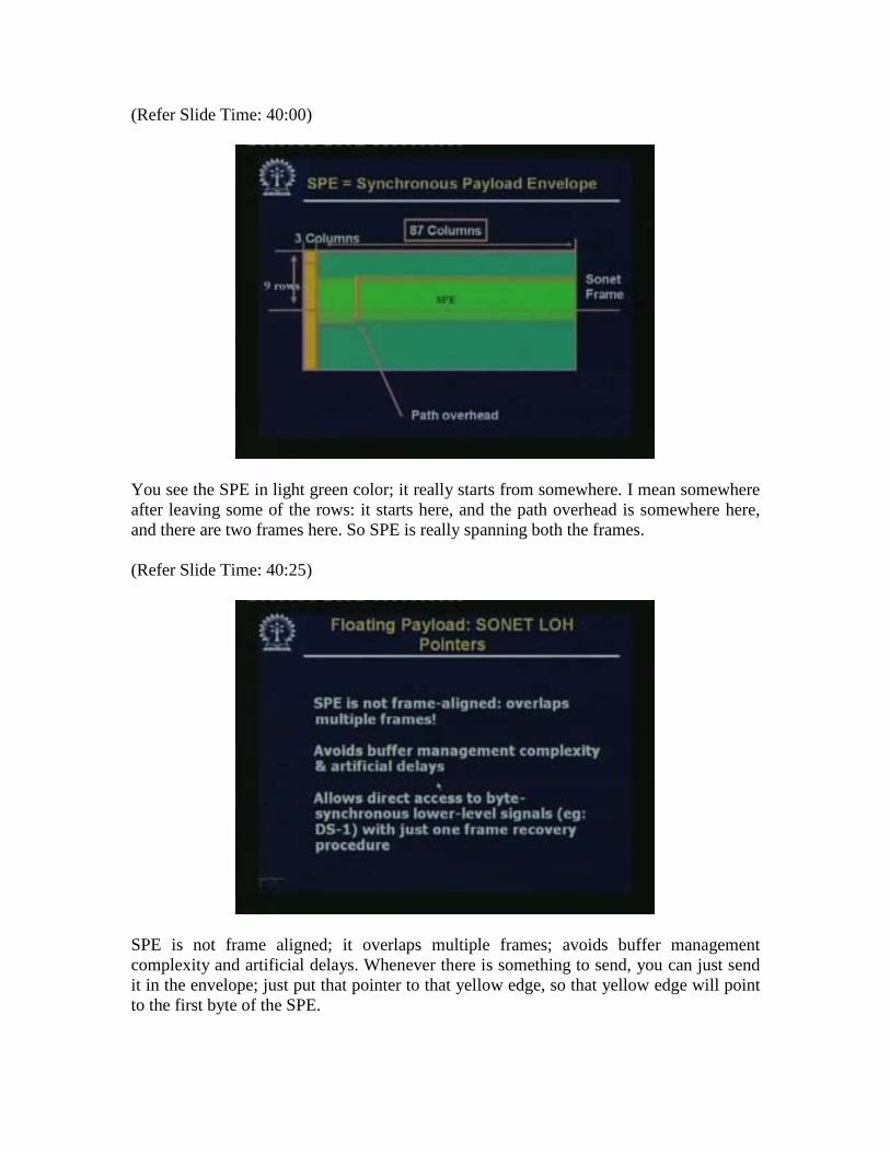
You see the SPE in light green color; it really starts from somewhere. I mean somewhere after leaving some of the rows: it starts here, and the path overhead is somewhere here, and there are two frames here. So SPE is really spanning both the frames. (Refer Slide Time: 40:25)

SPE is not frame aligned; it overlaps multiple frames; avoids buffer management complexity and artificial delays. Whenever there is something to send, you can just send it in the envelope; just put that pointer to that yellow edge, so that yellow edge will point to the first byte of the SPE.

It allows direct access to byte synchronous lower level signals, for example, DS1, with just one frame recovery procedure. (Refer Slide Time: 40:5 7)

These are the advantages of the SONET frames. This is one frame coming in may be 125 microseconds; this is the next frame; and SPE, as I have already shown, can overlap. I mean it may start somewhere within the first frame and then continue in the second frame in this fashion and then be over here. Actually after this, some other envelope may come in over here. (Refer Slide Time: 41:35)

Now of course where is the path overhead? There are two fields, H1 and H2 in LOH; LOH means line overhead, which points to the beginning of the path overhead. Path overhead beginning floats within the frame; 9 bytes that is one column may span frame along with the SPE; it is originated and terminated by all path devices; and this gives you end-to-end support. These are the features of path overhead. The point is that if you remember the path is end to end, that means it is close to the end users; just as the end user may start somewhere arbitrarily in-between, a path overhead also goes along with the SPE and it starts over there and at LOH, we keep a pointer to this path overhead. (Refer Slide Time: 42:40)

Just as some of the equipment that we use in SONET, one of the most important of these is the add drop multiplexer. They are important because at certain point in the network, what might happen is that there are some sources which want to send into the network. They will sort of go so there is this SONET equipment, which is ADM let us say, and SONET stream is flowing let us say like this. There may be something that wants to upload and travel along with this thing. At the same time, this may be the destination location for some of the other signals which originated elsewhere; they have to be dropped here. So some signals have to be dropped, some signals have to be added. So this multiplexer can handle that and that is very important. That is why they are called add drop multiplexers. This stream is itself of course flowing at a tremendous rate, whatever that rate is. So SONET SDH is a synchronous system with the master clock accuracy of 1 in 109, which you will see is highly accurate. It shows when you come in some kind of CCM clock somewhere and then there is a protocol for distributing and maintaining this clock over the entire network. Frames are sent byte by byte and ADMs can add drop smaller tributaries into the main SONET SDH stream and I have explained how that is done. Within that frame you can send lot of bytes; you can take out some of the bytes and add some of the bytes.

That is how you take out some of the smaller tributaries and add some of the smaller tributaries. (Refer Slide Time: 44:22)

Digital cross connect, which is an optical layer equipment, is also very important. It cross connects thousands of streams and software control, so it replaces patch panel; that is a good thing about the digital cross connect and a software control is coming where the control is coming from the control plane of the switches. You can connect the streams from may be one fiber to another; it handles performance monitoring, PDH SONET streams, and also provides ADM functions; that means add drop multiplexing functions. (Refer Slide Time: 44:58)

Finally we have this concept of grooming in SONET. Grooming means, we group the traffic in some format. So you want to keep this group in one particular way; it could be that there is a one group of streams for whom you want to give higher priority or you want to give higher quality of service. So you have to group them together. Similarly there may be multiple groups; so it enables grouping traffic with similar destination, Quos, etc., which is a part of grooming. It enables multiplexing or extracting streams also – that is also part of grooming. Narrow wider broadband and optical cross connects may be used for grooming. (Refer Slide Time: 45:47)

If you look at this figure, you have this narrow band, this SONET layer and optical layer. In the narrow band, we have this DS0 grooming and then in the DS1 grooming, there is a white band and then the broadband DS3 grooming – so the rates are going up, starting from the 64 kbps, it is going up. When you are going up for the STS 48, you are in optical domain; that means STS 48 is STM 16, so that is a high rate. The point is that, at that rate, most probably, you are well in the optical domain. Then, finally, you can go to all optical domain; that means wavelength, waveband, and fiber grooming – there are different levels of grooming, depending on what you want to do. Lastly we will just talk a little bit about virtual tributaries or containers. We have already talked a little bit about it. This is the opposite of STM; actually in some sense this is called sub multiplexing; that is, different streams coming together to form one very fat or very fast stream.


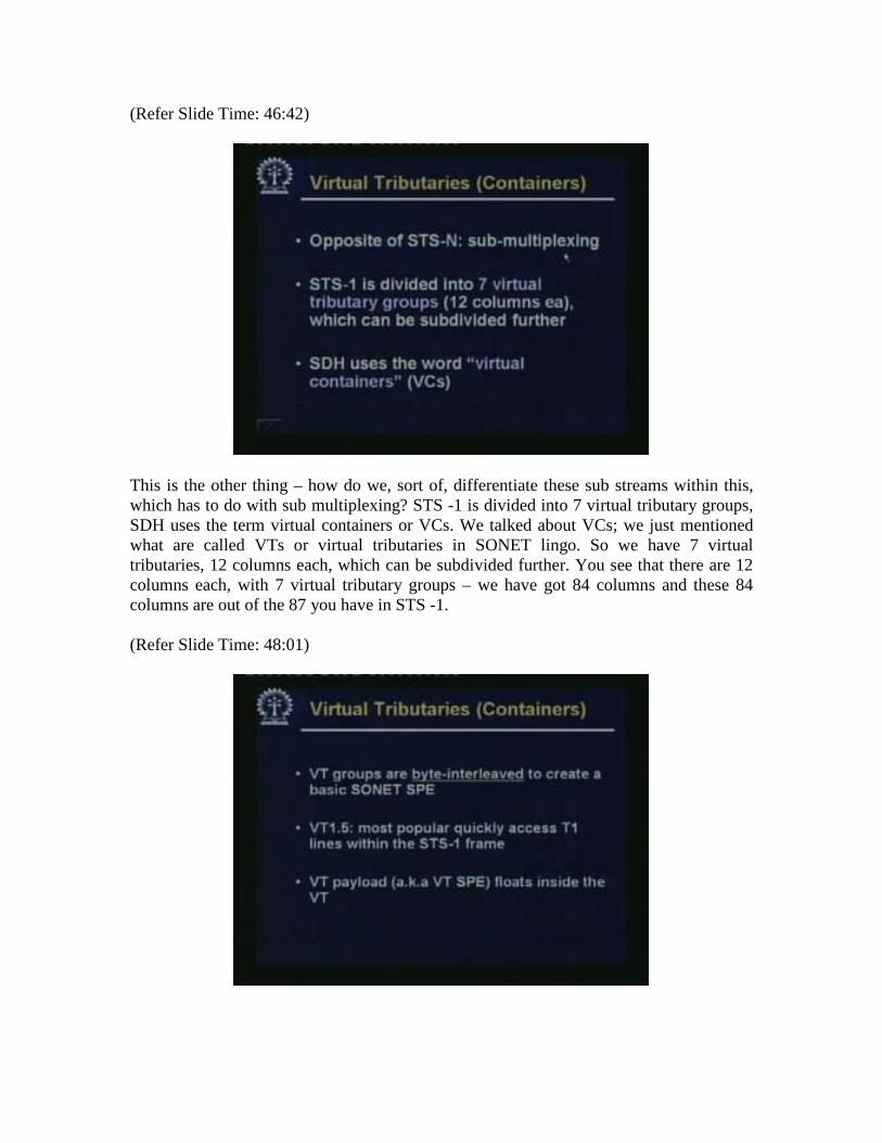
This is the other thing – how do we, sort of, differentiate these sub streams within this, which has to do with sub multiplexing? STS -1 is divided into 7 virtual tributary groups, SDH uses the term virtual containers or VCs. We talked about VCs; we just mentioned what are called VTs or virtual tributaries in SONET lingo. So we have 7 virtual tributaries, 12 columns each, which can be subdivided further. You see that there are 12 columns each, with 7 virtual tributary groups – we have got 84 columns and these 84 columns are out of the 87 you have in STS -1. (Refer Slide Time: 48:01)

VT groups are byte interleaved to create a basic SONET SPE. So this VT groups are byte interleaved. They may be again extracted from each other. VT 1.5 is the most popular, quickly accessed, T1 line within the STS-1 frame. So the idea is that you have a T1 line, which is approximately 1.5 mbps line, which is coming out of your small business, and you have a 1.5 mbps line. So that is your bandwidth requirement, you want to connect it to a distant location somewhere. And you do not want your thing to get mixed up with others. At the same time, as a small business you cannot have infrastructure of connecting to another location which is wide apart. So you will go with this public infrastructure or public switched tele PSDN network or whoever is maintaining this communication equipment. Usually telecom people maintain it in most of the places. Anyway, they have a sort of fiber going from one place to another, which contains very high-speed links. What you want is your T1 line should join them, sort of get transported over the distance and then go and feed into another T1 line at the destination. That is what you want. You want your T1 line to sort of have a separate sort of existence – just like in a compartment, we have different passengers. Passengers have their own individual entity but together they are packed into one compartment and then they travel. Similarly your T1 line is going to ride onto to this very fast stream and travel to the destination. So VT 1.5 gives your T1 line. (Refer Slide Time: 50:00)

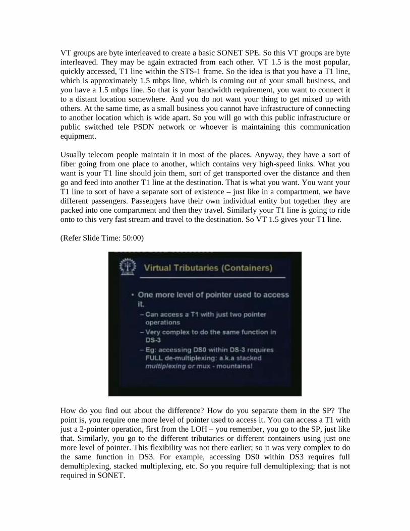
How do you find out about the difference? How do you separate them in the SP? The point is, you require one more level of pointer used to access it. You can access a T1 with just a 2-pointer operation, first from the LOH – you remember, you go to the SP, just like that. Similarly, you go to the different tributaries or different containers using just one more level of pointer. This flexibility was not there earlier; so it was very complex to do the same function in DS3. For example, accessing DS0 within DS3 requires full demultiplexing, stacked multiplexing, etc. So you require full demultiplexing; that is not required in SONET.

The point is that the other streams may go; you know where in that frame your bytes really are traveling for the stream or for the container or for the tributary that you are interested; you just extract it, others keep on traveling as they are. So you do not demultiplex the whole thing and that gives a great advantage of add drop multiplexing. (Refer Slide Time: 51:16)

This is just a figure showing that you can have various types of lines, all feeding into the same infrastructure. You may have what we have put over here: DS1, which is 1.544 mbps, E1, 2.048 mbps, DSIC DS2, DS3, ATM .48.384, E4, which is 139.264 mbps, ATM is about 150 mbps, etc. They are sort of traveling; they are getting in different containers. From VT 1.5, different tributaries, that is 1. 5236 etc., form a VT group and ride on a higher strength or higher speed stream.


Just as I said, these are sort of identified through a pointer; so we have this transport overhead. We use some bytes for that out of those 87 columns we have. So we use some columns of that and then we put a pointer, which gives to the STS payload pointer. Then there is a VT pointer, virtual tributary pointer, and this much is the VT SPE within the overall STS-1 SPE, which is the payload. Even now SONET is the most widely used technology in wide area networking that is existing today. Of course, as you know, as technology grows, maybe we will go out of SONET. People are already talking about going out of SONET because one disadvantage of SONET is that its equipment tends to be expensive. Well, expensive compared to what we think today. What is cheap today and what we think is cheap today may sound very expensive tomorrow; that is how the technology grows. So people are talking about direct transport over the optical layer, etc. May be we will touch those aspects later on. But all that is still in a sort of experimental stage and on the field, actually, SDH or SONET equipment is almost everywhere; all types of telephone companies are connected through that and major service providers use this as a means of transport. Thank you.



Good day, so today we will be speaking about fiber optic components and fiber optic communication as might of heard this lecture as well as the next couple of lectures, we will concentrate on fiber optic components. We have looked at some of the physical layer components of fiber optic systems before so we will sort of quickly review that, some of the stuff we will be talking about today is going to be common and then from that point.

we will take out take it up into WDM systems, how wavelength division multiplexing is done and how systems are handled in fiber optic domain, this fiber optic domain happens to be very crucial because a lot of traffic in terms of volume may be as much as forty to fifty percent, actually goes through the fiber as days are going by and as more and more demand for bandwidth is coming up fiber optics is becoming more and more important , we will be talking about fiber optic components today. (Refer Slide Time: 55:22)

In fiber optic component of course the basic fiber is there we have already talked about it, so we will talk little bit more about this then we have light source and receivers on two end because we know that in fiber optic cables light is the carrier of information then we require these different components like amplifiers, couplers, modulator, multiplexer and switches so we will look up at these components one by one and then we will start our discussion on wavelength division multiplexing.


The next set of components are multiplexers filters gratings, just talk little bit about it ,if you look at this wavelength , these are all; wavelength selective , devices multiplexers, filters , these are wavelength selective devices in a wavelength filter and what we want is suppose λ1, λ2 etc so many are coming, I want only λ 1 out 2 λ3 λ 4 etc are absorbed or something where as if you are a multiplexer I want the difference this λ coming in different lines, I want all to be mixed together and use the same line, these are wavelength multiplexer so application could be particular wavelength or a particular wave band selection. (Refer Slide Time: 56:42)

Wave band is nothing but some contiguous operating wavelengths which all are side by side, if you remember that in the operating window what ever be that 1550 what ever may be the window you are using there you can have a number of λ all side by side, there is a guard band between each of these operating λ so where the guard band that is given by the i q t has specified, how much guard band etc you have to have but so you can have large number of λ all group together in the same window. Aband out of that means a bunch of sequence is out of that you can short select instead of selecting only, that is wavelength band selection static wavelength cross connects and OAM is optical add drop multiplexers, you have come across this term optical add drop multiplexers in the context of Sonet but optical domain we require optical add drop multiplexers, we will come to that. Equalization of gain so that is another application filtering of noise ideas used in laser operation and dispersion compensation modules etc, these are the different applications one of the standard wavelength selective component is arrayed waveguide gratings ,we have seen this before… (Refer Slide Time: 58:08)

Computer Networks Prof. Sujoy Ghosh Department of Computer...

Documents

Transcript of Computer Networks Prof. Sujoy Ghosh Department of Computer...