
COMPUTER NETWORKS - II...COMPUTER NETWORKS - II (Subject Code: 10CS64) PART - A ... Behrouz A....
250
Computer Networks-II 10CS64 COMPUTER NETWORKS - II (Subject Code: 10CS64) PART - A UNIT-1 6 Hours Packet Switching Networks - 1: Network services and internal network operation, Packet network topology, Routing in Packet networks, shortest path routing: Bellman-Ford algorithm. UNIT–2 6 Hours Packet Switching Networks – 2: Shortest path routing (continued), Traffic management at the Packet level, Traffic management at Flow level, Traffic management at flow aggregate level. UNIT–3 6 Hours TCP/IP-1: TCP/IP architecture, The Internet Protocol, IPv6, UDP. UNIT–4 8 Hours TCP/IP-2: TCP, Internet Routing Protocols, Multicast Routing, DHCP, NAT and Mobile IP Dept Of CSE,SJBIT Page 1
Transcript of COMPUTER NETWORKS - II...COMPUTER NETWORKS - II (Subject Code: 10CS64) PART - A ... Behrouz A....

Computer Networks-II 10CS64
COMPUTER NETWORKS - II
(Subject Code: 10CS64)
PART - A
UNIT-1 6 Hours
Packet Switching Networks - 1: Network services and internal network
operation, Packet network topology, Routing in Packet networks, shortest path
routing: Bellman-Ford algorithm.
UNIT–2 6 Hours
Packet Switching Networks – 2: Shortest path routing (continued), Traffic
management at the Packet level, Traffic management at Flow level, Traffic
management at flow aggregate level.
UNIT–3 6 Hours
TCP/IP-1: TCP/IP architecture, The Internet Protocol, IPv6, UDP.
UNIT–4 8 Hours
TCP/IP-2: TCP, Internet Routing Protocols, Multicast Routing, DHCP, NAT
and Mobile IP
Dept Of CSE,SJBIT Page 1
Computer Networks-II 10CS64
PART – B
UNIT-5 7 Hours
Applications, Network Management, Network Security: Application layer
overview, Domain Name System (DNS), Remote Login Protocols, E-mail, File
Transfer and FTP, World Wide Web and HTTP, Network management, Overview
of network security, Overview of security methods, Secret-key encryption
protocols, Public-key encryption protocols, Authentication, Authentication and
digital signature, Firewalls.
UNIT–6 6 Hours
QoS, VPNs, Tunneling, Overlay Networks: Overview of QoS, Integrated
Services QoS, Differentiated services QoS, Virtual Private Networks, MPLS,
Overlay networks.
UNIT-7 7 Hours
Multimedia Networking: Overview of data compression, Digital voice and
compression, JPEG, MPEG, Limits of compression with loss, Compression
methods without loss, Overview of IP Telephony, VoIP signaling protocols, Real-
Time Media Transport Protocols, Stream control Transmission Protocol (SCTP)
UNIT–8 6 Hours
Mobile AdHoc Networks and Wireless Sensor Neworks: Overview of Wireless
Ad-Hoc networks, Routing in AdHOc Networks, Routing protocols for and
Dept Of CSE,SJBIT Page 2

Computer Networks-II 10CS64
Security of AdHoc networks, Sensor Networks and protocol structures,
Communication Energy model, Clustering protocols, Routing protocols, ZigBee
technology and 802.15.4.
Text Books:
1. Communication Networks – Fundamental Concepts & key architectures,
Alberto Leon Garcia & Indra Widjaja, 2nd Edition, Tata McGraw-Hill, India (7 -
excluding 7.6, 8)
2. Computer & Communication Networks, Nadir F Mir, Pearson Education, India
(9, 10 excluding 10.7, 12.1 to 12.3, 16, 17.1 to 17.6, 18.1 to18.3, 18.5, 19, 20)
Reference Books:
1. Behrouz A. Forouzan: Data Communications and Networking, 4th Edition, Tata
McGraw-Hill, 2006.
2. William Stallings: Data and Computer Communication, 8th Edition, Pearson
Education, 2007.
3. Larry L Peterson and Bruce S Davie: Computer Networks – A Systems
Approach, 4th Edition, Elsevier, 2007.
4. Wayne Tomasi: Introduction to Data Communications and Networking, Pearson
Education, 2005.
Dept Of CSE,SJBIT Page 3

Computer Networks-II 10CS64
TABLE OF CONTENTS
PART-A
UNIT - 1 Packet Switching Networks – 1……………………………….6-29
UNIT – 2 Packet Switching Networks – 2……………………………...30-42
UNIT – 3 TCP/IP-1……………………………………………………...43-58
UNIT – 4 TCP/IP-2……………………………………………………...59-90
PART – B
UNIT – 5 Applications, Network Management, Network Security….92-145
UNIT – 6 QoS, VPNs, Tunneling, Overlay Networks………………146-172
UNIT - 7 Multimedia Networking……………………………………173-215
UNIT – 8 Mobile AdHoc Networks and Wireless Sensor Neworks..216-250
Dept Of CSE,SJBIT Page 4

Computer Networks-II 10CS64
PART-A
Dept Of CSE,SJBIT Page 5

Computer Networks-II 10CS64
UNIT - 1
Packet Switching Networks - 1: Network services and internal
network operation, Packet network topology, Routing in Packet
networks, shortest path routing: Bellman-Ford algorithm.
Dept Of CSE,SJBIT Page 6
Computer Networks-II 10CS64
UNIT-I
PACKET-SWITCHING NETWORKS:
In Circuit switching the resources allocated for a particular
user can not be used by other users at the same time. This approach
is inefficient when the amount of information transferred is small
or if information is produced in bursts, as is the case in many
computer applications. Networks that transfer blocks of
information called packets. Packet-switching networks are better
matched to computer applications and can also be designed to
support real-time applications such as telephony.
1.1 Packet networks can be viewed by two perspectives:
One perspective involves an external view of the network
and is concerned with the services that the network provides to
the transport layer that operates above it at the end systems.
Ideally the definition of the network services is independent of the
underlying network and transmission technologies. This approach
allows the transport layer and the applications that operate above
it to be designed so that they can function over any network that
provides the given services.
A second perspective on packet networks is concerned with
the internal operation of a network. Here look at the physical
topology of a network, the interconnection of links, switches, and
routers. The approach that is used to direct information across
the network: datagrams, or virtual circuits. The first perspective,
involving the services provided to the layer above, does not differ
in a fundamental way between broadcast and switched packet
networks.
The second perspective, however, is substantially different.
Dept Of CSE,SJBIT Page 7

Computer Networks-II 10CS64
In the case of LANs, the network is small, addressing is simple,
and the frame is transferred in one hop so no routing is required.
In the case of packet-switching networks, addressing must
accommodate extremely large-scale networks and must work in
concert with appropriate routing algorithms. These two
challenges, addressing and routing, are the essence of the
network layer.
NETWORK SERVICES AND INTERNAL NETWORK
OPERATION:
The essential function of a network is to transfer
information among the users that are attached to the network or
internetwork. In Figure 1.1 we show that this transfer may involve
a single block of information or a sequence of blocks that are
temporally related. In the case of a single block of information,
we are interested in having the block delivered correctly to the
destination, and we may also be interested in the delay
experienced in traversing the network. In the case of a sequence of
blocks, we may be interested not only in receiving the blocks
correctly and in the right sequence but also in delivering a
relatively unimpaired temporal relation.
Figure 1.2 shows a transport protocol that operates end to
end across a network. The transport layer peer processes at the
end systems accept messages from their higher layer and transfer
these messages by exchanging segments end to end across the
network. The f i gure shows the interface at which the network
service is visible to the transport layer. The network service is all
that matters to the transport layer, and the manner in which the
network operates to provide the service is irrelevant.
The network service can be connection-oriented or
connectionless. A con- nectionless service is very simple, with
only two basic interactions between the transport layer and the
Dept Of CSE,SJBIT Page 8
Computer Networks-II 10CS64
network layer: a request to the network that it send a packet and
an indication from the network that a packet has arrived. The
user can request transmission of a packet at any time, and does not
need to inform the network layer that the user intends to transmit
information ahead of time.
A connection-release procedure may also be required to
terminate the connection. It is clear that providing connection-
oriented service entails greater complexity than connectionless
service in the network layer.
It is also possible for a network layer to provide a choice of
services to the user of the network. For example, the network
layer could offer:
i) best-effort connectionless service
ii) low-delay connectionless service
iii) connection-oriented reliable stream service
iv) connection-oriented transfer of packet with delay and
bandwidth guarantees.
t0 t1
Network
FIGURE 1.1 A network transfers information among user
Dept Of CSE,SJBIT Page 9

Computer Networks-II
Messages
Transport layer
Network
layer
Data link
layer
Physical
layer
Peer-to-peer protocols
across a network protocol stack view
It is easy to come up with examples of applications that can
make use of each of these services. However, it does not follow
that all the services should be offered by the network layer.
When applied to the issue of choice of network services,
the end-to-end argument suggests that functions should be
placed as close to the application as possible, since it is the
Dept Of CSE,SJBIT Page10
Transport layer
Network
layer
Data link
layer
Physical
layer
Segments
Network service
End system
a
Network service
End system
b
Network layer
Data link
layer
Physical
layer Network
layer
Data link
layer
Physical
layer
operating end to end FIGURE 1.2
10CS64
Messages
Computer Networks-II 10CS64
application that is in the best position to determine whether a
function is being carried out completely and correctly. This
argument suggests that as much functionality as possible should
be located in the transport layer or higher and that the network
services should provide the minimum functionality required to
meet application performance.
Consider the internal operation of the network. Figure 1 .3
shows the relation between the service offered by the network
and the internal operation. T he internal operation of a network
is connectionless if packets are transferred within the network as
datagrams. Thus in the figure each packet is routed
independently. Consequently packets may follow different paths
from to and so may arrive out of order. We say that the
internal operation of a network is connection-oriented if packets
follow virtual circuits that have been established from a source
to a destination. Thus to provide communications between
and, routing to set up a virtual circuit is done once, and
thereafter packets are simply forwarded along the established
path. If resources are reserved during connection setup, then
bandwidth, delay, and loss guarantees can be provided.
The fact that a network offers connection-oriented service,
connectionless service, or both does not dictate how the network
must operate internally.
Dept Of CSE,SJBIT Page 11

Computer Networks-II 10CS64
C
Medium
1 2 3 2 1 Network
Physical layer entity
3
Data link layer entity
End system
Network layer entity
Transport layer entity
entities work together to provide network
service to layer 4 entities
Dept Of CSE,SJBIT Page 13
A
1 2 1 2 3 2 1
B
3
Network layer entity
4
End
b
3 2 1 1 2 3
system
a
4 3 2 1
1
2
FIGURE 1.3 Layer 3

Computer Networks-II 10CS64
This reasoning suggests a preference for a connectionless
network, which has much lower complexity than a connection-
oriented network. The reasoning does allow the possibility for
some degree of ``connection orientation'' as a means to ensure that
applications can receive the proper level of performance. Indeed
current research and standardization efforts can be viewed as an
attempt in this direction to determine an appropriate set of network
services and an appropriate mode of internal network operation.
We have concentrated on high-level arguments up to this
point. Clearly, functions that need to be carried out at every node
in the network must be in the network layer. Thus functions that
route and forward packets need to be done in the network layer.
Priority and scheduling functions that direct how packets are
forwarded so that quality of service is provided also need to be in
the network layer. Functions that belong in the edge should, if
possible, be imple- mented in the transport layer or higher. A
third category of functions can be implemented either at the edge
or inside the network. For example, while con- gestion takes place
inside the network, the remedy involves reducing input flows at the
edge of the network. We will see that congestion control has been
imple- mented in the transport layer and in the network layer.
Dept Of CSE,SJBIT Page 14
Computer Networks-II 10CS64
The network layer may therefore be called upon to carry out
segmentation inside the network and reassembly at the edge.
Alternatively, the network could send error messages to the
sending edge, requesting that the packet size be reduced. A more
challenging set of functions arises when the ``network'' itself may
actually be an internetwork. In this case the network layer must also
be concerned not only about differences in the size of the units that
the component networks can transfer but also about differences
in addressing and in the services that the component networks
provide.
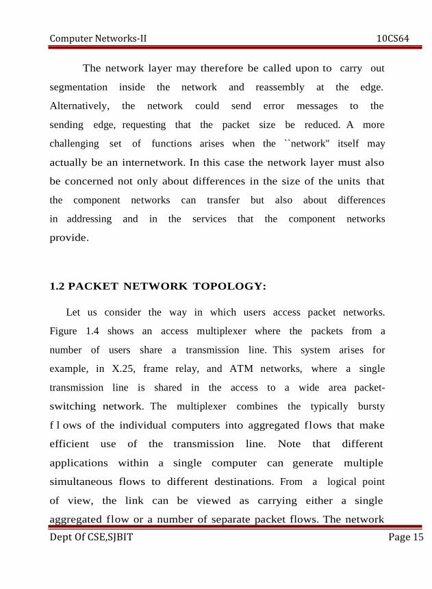
1.2 PACKET NETWORK TOPOLOGY:
Let us consider the way in which users access packet networks.
Figure 1.4 shows an access multiplexer where the packets from a
number of users share a transmission line. This system arises for
example, in X.25, frame relay, and ATM networks, where a single
transmission line is shared in the access to a wide area packet-
switching network. The multiplexer combines the typically bursty
f l ows of the individual computers into aggregated flows that make
efficient use of the transmission line. Note that different
applications within a single computer can generate multiple
simultaneous flows to different destinations. From a logical point
of view, the link can be viewed as carrying either a single
aggregated flow or a number of separate packet flows. The network
Dept Of CSE,SJBIT Page 15

Computer Networks-II 10CS64
access node forwards packets into a backbone packet network.
Network access
MUX
LANs provide the access to packet-switching networks in many
environments. As shown in Figure 1.5a, computers are connected
to a shared transmission medium. Transmissions are broadcast to
all computers in the network. Each computer is identified by a
unique physical address, and so each station listens for its address
to receive transmissions. Broadcast and multi- cast transmissions
are easily provided in this environment.
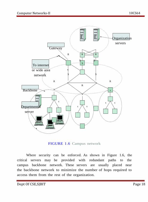
Multiple LANs in an organization, in turn, are interconnected
into campus networks with a structure such as that shown in
Figure 1 .6. LANs for a large group of users such as a
department are interconnected in an extended LAN through the
use of LAN switches, identified by lowercase s in the figure.
Resources such as servers and databases that are primarily of
use to this department are kept within the subnetwork. This
approach reduces delays in accessing the resources and contains
the level of trafic that leaves the subnetwork. Each subnetwork
has access to the rest of the organization through a router R that
Dept Of CSE,SJBIT Page 16

Computer Networks-II 10CS64
accesses the campus backbone network. A subnetwork also uses
the campus backbone to reach the ``outside world'' such as the
Internet or other sites belong- ing to the organization through a
gateway router. Depending on the type of organization, the
gateway may implement firewall functions to control the traffic
that is allowed into and out of the campus network.
Servers containing critical resources that are required by the
entire organization are usually located in a data center where they
can be easily maintained and
(a) (b)
LAN LAN 1
Bridge
LAN 2
FIGURE 1.5 Local area networks
Dept Of CSE,SJBIT Page 17
Computer Networks-II
Gateway
To internet
or wide area
network
R
Backbone
Departmental
server
FIGURE 1.6 Campus network
Where security can be enforced. As shown in Figure 1.6, the
critical servers may be provided with redundant paths to the
campus backbone network. These servers are usually placed near
the backbone network to minimize the number of hops required to
access them from the rest of the organization.
Dept Of CSE,SJBIT Page 18
s
s
R
S
s
10CS64
Organization
servers
R R
s s S
S
R
R
s
s
s s
s
Computer Networks-II 10CS64
The trafic within an extended LAN is delivered based on the
physical LAN addresses. However, applications in host computers
operate on the basis of logical IP addresses. Therefore, the
physical address corresponding to an IP address needs to be
determined every time an IP packet is to be transmitted over a
LAN. This address resolution problem can be solved by using IP
address to physical address translation tables.
The routers in the campus network are interconnected to form
the campus backbone network, depicted by the mesh of switches,
designated S, in Figure 1.6. Typically, for large organizations such
as universities these routers are interconnected by using very high
speed LANs, for example, Gigabit Ethernet or an ATM network.
The routers use the Internet Protocol (IP), which enables them to
operate over various data link and network technologies. The
routers exchange information about the state of their links to
dynamically calculate routing tables that direct packets across the
campus network. The routers in the campus network form a
domain or autonomous system. The term domain indicates that the
routers run the same routing protocol. The term autonomous system
is used for one or more domains under a single administration.
Organizations with multiple sites may have their various
campus networks interconnected through routers interconnected
by leased digital transmission lines or frame relay connections.
In this case access to the wide area network may use an access
multiplexer such as the one shown in Figure 1 .4. In addition the
campus network may be connected to an Internet service provider
through one or more border routers as shown in Figure 1 .7. To
communicate with other networks, the autonomous system must
Dept Of CSE,SJBIT Page 19

Computer Networks-II 10CS64
provide information about its network routes in the border
routers.
A national ISP provides points of presence in various
cities where customers can connect to their network. The ISP has
its own national network for interconnecting its POPs. This
network could be based on ATM; it might use IP over SONET; or
it might use some other network technology. The ISPs in turn
exchange traffic as network access points (NAPs), as shown in
Figure 1.8a. A NAP is a high-speed LAN or switch at which the
routers from different ISPs
Interdomain level
Border routers
Border routers
Autonomous
system or
domain
LAN level Intradomain level
FIGURE 1.7 Intradomain and
Dept Of CSE,SJBIT
Internet service provider
interdomain levels
Page 20

Computer Networks-II 10CS64
(a) National service provider A
National service provider B
NAP
National service provider C
RB
(b)
NAP
RA
Route
server
LAN
RC
FIGURE 1.8 National ISPs exchange traffic at NAPs
Dept Of CSE,SJBIT Page21
NAP

Computer Networks-II 10CS64
Routing information is exchanged through route servers can
exchange trafic, and as such NAPs are crucial to the
interconnectivity provided by the Internet.
Thus we see that a multilevel hierarchical network topology
arises for the Internet which is much more decentralized than
traditional telephone networks. This topology comprises multiple
domains consisting of routers interconnected by point-to-point
data links, LANs, and wide area networks such as ATM. The
principal task of a packet-switching network is to provide
connectivity among users. The routing protocols must adapt to
changes in network topology due to the introduction of new
nodes and links or to failures in equipment. Different routing
algorithms are used within a domain and between domains.
1.3 Routing in packet networks:
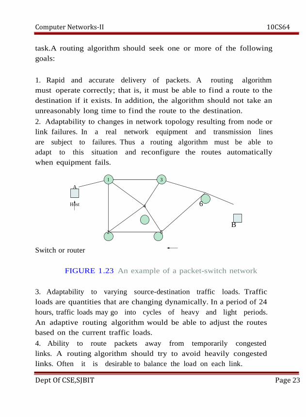
A packet-switched network consists of nodes (routers or
switches) intercom nected by communication links in an arbitrary
meshlike fashion as shown in Figure 1.23. As suggested by the
figure, a packet could take several possible paths from host A to
host B. For example, three possible paths are 1-3-6, 1-4-5-6, and 1-
2-5-6. However, which path is the ``best''one?
If the objective is to minimize the number of hops, then path
1-3-6 is the best. If each link incurs a certain delay and the
objective function is to minimize the end-to-end delay, then the
best path is the one that gives the end-to-end minimum delay.
Yet a third objective function involves selecting the path with the
greatest available bandwidth. The purpose of the routing algorithm
is to identify the set of paths that are best in a sense defined by
the network operator. Note that a routing algorithm must have
global knowledge about the network state in order to perform its
Dept Of CSE,SJBIT Page 22
Computer Networks-II 10CS64
task.A routing algorithm should seek one or more of the following
goals:
1. Rapid and accurate delivery of packets. A routing algorithm
must operate correctly; that is, it must be able to find a route to the
destination if it exists. In addition, the algorithm should not take an
unreasonably long time to find the route to the destination.
2. Adaptability to changes in network topology resulting from node or
link failures. In a real network equipment and transmission lines
are subject to failures. Thus a routing algorithm must be able to
adapt to this situation and
when equipment fails.
1
A
Host
2
Switch or router
FIGURE 1.23 An example of a packet-switch network
3. Adaptability to varying source-destination traffic loads. Traffic
loads are quantities that are changing dynamically. In a period of 24
hours, traffic loads may go into cycles of heavy and light periods.
An adaptive routing algorithm would be able to adjust the routes
based on the current traffic loads.
4. Ability to route packets away from temporarily congested
links. A routing algorithm should try to avoid heavily congested
links. Often it is desirable to balance the load on each link.
Dept Of CSE,SJBIT Page 23
reconfigure the
3
4
5
routes automatically
6
B
Computer Networks-II 10CS64
5. Ability to determine the connectivity of the network. To find
optimal routes, the routing system needs to know the connectivity
or reachability information.
6. Low overhead. A routing system typically obtains the
connectivity information by exchanging control messages with
other routing systems. These messages represent an overhead that
should be minimized.
Routing Algorithm Classification
One can classify routing algorithms in several ways. Based on
their responsive ness, routing can be static or dynamic (or
adaptive). In static routing the network topology determines the
initial paths. The precomputed paths are then manually loaded to
the routing table and remain fixed for a relatively long period of
time. Static routing may suffice if the network topology is
relatively fixed and the network size is small. Static routing
becomes cumbersome as the network size increases. The biggest
disadvantage of static routing is its inability to react rapidly to
network failures. In dynamic (adaptive) routing each router
continu ously learns the state of the network by communicating
with its neighbors. Thus a change in a network topology is
eventually propagated to all the routers. Based on the information
collected, each router can compute the best paths to desired
destinations. One disadvantage of dynamic routing is the added
complexity in the router.
A routing decision can be made on a per packet basis or during
the connec tion setup time. With virtual-circuit packet switching,
the path (virtual circuit) is determined during the connection setup
phase. Once the virtual circuit is established, all packets
belonging to the virtual circuit follow the same route.
Dept Of CSE,SJBIT Page 24
Computer Networks-II 10CS64
Datagram packet switching does not require a connection setup.
The route followed by each packet is determined independently.
Shortest-path algorithms:
Network routing is a major component at the network layer
and is concerned with the problem of determining feasible paths
(or routes) from each source to each destination. A router or a
packet-switched node performs two main functions: routing and
forwarding.
In the routing function an algorithm finds an optimal path to
each destination and stores the result in a routing table. In the
forwarding function a router forwards each packet from an input
port to the appropriate output port based on the information stored
in the routing table.
Shortest-path routing algorithms: the Bellman-Ford algorithm
and Dijkstra's algorithm.Some other routing approaches are
flooding, deflection routing, and source routing.
Most routing algorithms are based on variants of shortest-path
algorithms,which try to determine the shortest path for a packet
according to some cost criterion. To better understand the purpose
of these algorithms, consider a communication network as a graph
consisting of a set of nodes (or vertices) and a set of links (or edges,
arcs, or branches), where each node represents a router or a packet
switch and each link represents a communication channel between
two routers. Figure 1.28 shows such an example. Associated with
each link is a value that represents the cost of using that link. For
simplicity, it is assumed that each link is nondirected. If a link is
directed, then the cost must be assigned to each direction. If we
define the path cost to be the sum of the link costs along the path,
then the shortest path between a pair of nodes is the path with the
Dept Of CSE,SJBIT Page 25

Computer Networks-II 10CS64
least cost. For example, the shortest path from node 2 to node 6 is
2-4-3-6, and the path cost is 4.
FIGURE 1.28 A sample network with
associated link costs
assign a cost to each link,
depending on which function is to be optimized. Examples include
1. Cost 1/capacity. The cost is inversely proportional to the
link capacity. Here one assigns higher costs to lower-capacity
links. The objective is to send a packet through a path with the
highest capacity. If each link has equal capacity, then the shortest
path is the path with the minimum number of hops.
2. Cost packet delay. The cost is proportional to an average
packet delay, which includes queueing delay in the switch buffer
and propagation delay in the link. The shortest path represents the
fastest path to reach the destination.
3. Cost congestion. The cost is proportional to some congestion
measure, for example, traffic loading. Thus the shortest path tries to
avoid congested links.
The Bellman-Ford Algorithm
The Bellman-Ford algorithm (also called the Ford-Fulkerson
algorithm) is based on a principle that is intuitively easy to
understand: If a node is in the shortest path between A and B,
Dept Of CSE,SJBIT Page 26
2
5
1
4
Many
3
2
4
3
5
metrics
1
2
can be
1
3
2
6
used to

Computer Networks-II 10CS64
then the path from the node to A must be the shortest path and
the path from the node to B must also be the shortest path. As
an example, suppose that we want to find the shortest path from
node 2 to node 6 (the destination) in Figure 1 .28. To reach the
destination, a packet from node 2 must f i rst go through node 1,
node 4, or node 5. Suppose that someone tells us that the shortest
paths from nodes 1, 4, and 5 to the destination (node 6) are 3, 3,
and 2, respectively. If the packet first goes through node 1, the total
distance (also called total cost) is 3 + 3, which is equal to 6.
Through node 4, the total distance is 1 + 3, equal to 4. Through
node 5, the total distance is 4 + 2, equal to 6. Thus the shortest
path from node 2 to the destination node is achieved if the
packet first goes through node 4.
To formalize this idea, let us first fix the destination node. Define
Dj to be the current estimate of the minimum cost (or minimum
distance) from node j to the destination node and Cij to be the link
cost from node i to node j. For example, defined to be zero (that is,
Cii f l 0), and the link cost between node i and node k is infinite if
node i and node k are not directly connected. For example, C15 f l
C23 f l 1 in Figure 1.28. With all these definitions, the minimum cost
from node 2 to the destination node (node 6) can be calculated by
D2 fl min{C21 + D1, C24 + D4, C25 + D5 }
fl min{3 + 3, 1 + 3, 4 + 2}
fl 4
Thus the minimum cost from node 2 to node 6 is equal to 4, and the
next node to visit is node 4. One problem in our calculation of the
minimum cost from node 2 to node 6 is that we have assumed that
the minimum costs from nodes 1, 4, and 5 to the destination were
known. In general, these nodes would not know their mini-mum
Dept Of CSE,SJBIT Page 27

Computer Networks-II 10CS64
costs to the destination without performing similar calculations. So
let us apply the same principle to obtain the minimum costs for the
other nodes. For example,
D1 fl min{C12 + D2, C13 + D3, C14 + D4}
And D4 fl min{C41 + D1, C42 + D2, C43 + D3, C45 + D5}
A discerning reader will note immediately that these equations
are circular, since D2 depends on D1 and D1 depends on D2 . The
magic is that if we keep iterating and updating these equations, the
algorithm will eventually converge to the correct result. To see
this outcome, assume that initially D1 flD2 f l . . . fl D5 f l ∞ .
Observe that at each iteration, D1 , D2 , . . . , D5 are nonincreasing.
Because the minimum distances are bounded below, eventually
D1, D2, . . . , D5 must converge.
Now if we define the destination node, we can summarize the
Bellman-Ford algorithm as follows:
1. Initialization
Di fl∞; for all i ≠ d
Dd f l 0
2. Updating: For each i ≠ d,
Di fl mijn{Cij + Dj}, for all j ≠ i
Repeat step 2 until no more changes occur in the iteration.
Dept Of CSE,SJBIT Page 28

Computer Networks-II 10CS64
UNIT – 2
Packet Switching Networks – 2: Shortest path routing (continued),
Traffic management at the Packet level, Traffic management at Flow
level, Traffic management at flow aggregate level.
Dept Of CSE,SJBIT Page 29
Computer Networks-II 10CS64
UNIT – 2
PACKET SWITCHING NETWORKS – 2:
2.1 Traffic Management at the packet level:
Traffic management is concerned with the delivery of QoS
to specific packet flows. Traffic management entails mechanisms
for managing the flows in a network to control the load that is
applied to various links and switches. Traffic management also
involves the setting of priority and scheduling mechanisms at
switches, routers, and multiplexers to provide differentiated
treatment for packets and cells belonging to different classes,
flows, or connections. It also may involve the policing and
shaping of traffic flows as they enter the network.
The dashed arrows show packets from other flows that
``interfere''with the packet of interest in the sense of contending for
buffers and transmission along the path. We also note that these
interfering flows may enter at one multi- plexer and depart at some
later multiplexer, since in general they belong to different source-
destination pairs and follow different paths through the network.
The performance experienced by a packet along the path is the
accumulation of the performance experienced at the N
multiplexers. For example, the total end-to-end delay is the sum
of the delays experienced at each multiplexer. Therefore, the
average end-to-end delay is the sum of the individual average
delays. On the other hand, if we can guarantee that the delay at each
multiplexer can be kept below some upper bound, then the end-
to-end delay can be kept below the sum of the upper bounds at the
various multiplexers. The jitter experienced by packets is also of
interest. The jitter measures the variability in the packet delays and
is typically measured in terms of the difference of the minimum
Dept Of CSE,SJBIT Page 30

Computer Networks-II 10CS64
delay and some maximum value of delay.
Note that the discussion here is not limited solely to
connection-oriented packet transfer. In the case of connectionless
transfer of packets, each packet will experience the performance
along the path traversed. On the other hand, this analysis will hold in
connectionless packet switching networks for the period of time
during which a single path is used between a source and a
destination. If these paths can be ``pinned down'' for certain flows
in a connectionless network, then the end-to-end analysis is valid.
Packet-switching networks are called upon to support a wide
range of services with diverse QoS requirements. To meet the QoS
requirements of multiple services, an ATM or packet multiplexer
must implement strategies for managing how cells or packets are
placed in the queue or queues, as well as control the transmission
bit rates that are provided to the various information flows. We
now consider a number of these strategies.
1 2 N-1 N
FIGURE 1.41 The end-to-end QoS of a packet along a
path traversing N hops
Dept Of CSE,SJBIT Page31
Computer Networks-II 10CS64
2.2 Traffic management at Flow level:
FIFO and Priority Queues: The simplest approach to
managing a multiplexer involves first-in, first-out (FIFO) queuing
where all arriving packets are placed in a common queue and
transmitted in order of arrival, as shown in Figure 1.42a. Packets
are discarded when they arrive at a full buffer. The delay and loss
experienced by packets in a FIFO system depend on the inter
arrival times and on the packet lengths. As inter arrivals become
more bursty or packet lengths more variable, performance will
deteriorate. Because FIFO queuing treats all packets in the same
manner, it is not possible to provide different information flows
with different qualities of service. FIFO systems are also subject
to hogging, which occurs when a user sends packets at a high rate
and fills the buffers in the system, thus depriving other users of
access to the multiplexer.
A FIFO queuing system can be modified to provide different
packet-loss performance to different traffic types. Figure 1 .42b
shows an example with two classes of traffic. When the number of
packets reaches a certain threshold, arrivals of lower access
priority (Class 2) are not allowed into the system. Arrivals of higher
access priority (Class 1) are allowed as long as the buffer is not
full. As a result, packets of lower access priority will experience a
higher packet-loss probability.
Head-of-line (HOL) priority queuing is a second approach
that involves defining a number of priority classes. A separate
queue is maintained for each priority class. As shown in Figure
1.43, each time the transmission line becomes available the next
packet for transmission is selected from the head of the line of the
highest priority queue that is not empty.
For example, it does not allow for providing some egree of
guaranteed access to transmission bandwidth to the lower
Dept Of CSE,SJBIT Page 32

Computer Networks-II 10CS64
Another problem is that it does not discriminate
priority. Fairness problems can arise
user hogs the bandwidth by sending an
FIGURE 1.42 (a) FIFO queueing; (b)
Transmission link
Packet
discard
when full
Packet buffer
Transmission link
Class 1 Class 2
discard discard
when full when threshold
exceeded
Packet
discard
when full
High-priority packets
Low-priority packets
Dept Of CSE,SJBIT
users
priority classes.
between
here when a
of the same
certain
excessive number of packets.
(a)
Arriving packets
(b)
Arriving packets
Packet buffer
FIGURE 1 .43 HOL priority
Transmission link
Page 33

Computer Networks-II 10CS64
When
high-priority
queue empty
Packet
discard
when full
A third approach to managing a multiplexer, shown in Figure
1.44, involves sorting packets in the queue according to a priority
tag that reflects the urgency with which each packet needs to be
transmitted. This system is very flexible because the method for
defining priority is open and can even be defined dynamically. For
example, the priority tag could consist of a priority class followed
by the arrival time of a packet to a multiplexer.
A third important example that can be implemented by
the approach is fair queueing and weighted fair queueing, which are
discussed next.
Sorted packet buffer
Transmission link
Packet
discard
when full
FIGURE 7.44 Sorting packets according to priority tag
Dept Of CSE,SJBIT Page 34
Taggin g
Arriving packets
Computer Networks-II 10CS64
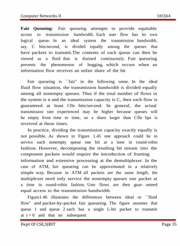
Fair Queueing: Fair queueing attempts to provide equitable
access to transmission bandwidth. Each user flow has its own
logical queue. In an ideal system the transmission bandwidth,
say, C bits/second, is divided equally among the queues that
have packets to transmit.The contents of each queue can then be
viewed as a fluid that is drained continuously. Fair queueing
prevents the phenomenon of hogging, which occurs when an
information flow receives an unfair share of the bit
Fair queueing is ``fair'' in the following sense. In the ideal
fluid flow situation, the transmission bandwidth is divided equally
among all nonempty queues. Thus if the total number of flows in
the system is n and the transmission capacity is C, then each flow is
guaranteed at least Cfln bits/second. In general, the actual
transmission rate experienced may be higher because queues will
be empty from time to time, so a share larger than Cfln bps is
received at those times.
In practice, dividing the transmission capacity exactly equally is
not possible. As shown in Figure 1.45 one approach could be to
service each nonempty queue one bit at a time in round-robin
fashion. However, decomposing the resulting bit stream into the
component packets would require the introduction of framing
information and extensive processing at the demultiplexer. In the
case of ATM, fair queueing can be approximated in a relatively
simple way. Because in ATM all packets are the same length, the
multiplexer need only service the nonempty queues one packet at
a time in round-robin fashion. User flows are then guar- anteed
equal access to the transmission bandwidth.
Figure1.46 illustrates the differences between ideal or ``fluid
flow'' and packet-by-packet fair queueing. The figure assumes that
queue 1 and queue 2 each has a single L-bit packet to transmit
at t = 0 and that no subsequent
Dept Of CSE,SJBIT Page 35

Computer Networks-II 10CS64
packets arrive. Assuming a capacity of C = L bits/second fl 1
packet/second,
the fluid-flow system transmits each
and therefore.
Packet flow 1
Packet flow 2
Packet flow n
FIGURE 1.45 Fair queueing
completes the transmission of both packets exactly at time t = 2
seconds. The bit-by-bit system (not shown in the figure) would
begin by transmitting one bit from queue 1, followed by one bit
from queue 2, and so on. On the other hand, the packet-by-packet
fair-queueing system transmits the packet from queue 1 first and
then transmits the packet from queue 2, so the packet completion
times are 1 and 2 seconds. In this case the first packet is 1 second
too early relative to the completion time in the fluid system.
Approximating fluid-flow fair queueing is not as straightforward
when pack- ets have variable lengths. If the different user queues are
serviced one packet at a time in round-robin fashion, we do not
necessarily obtain a fair allocation of transmission bandwidth. For
example, if the packets of one flow are twice the size of packets in
another flow, then in the long run the first flow will obtain twice
Dept Of CSE,SJBIT Page 36
packet at a rate of 1/2
Approximated
bit-level
round-robin
service
C bits/second
Transmission link
Computer Networks-II 10CS64
the bandwidth of the second flow. A better approach is to transmit
packets from the user queues so that the packet completion times
approximate those of a fluid- flow fair queueing system. Each time
a packet arrives at a user queue, the completion time of the
packet is derived from a fluid-flow fair-queueing system. This
number is used as a finish tag for the packet. Each time the
transmission of a packet is completed, the next packet to be
transmitted is the one with the smallest finish tag among all of the
user queues. We refer to this system as a packet-by-packet fair-
queueing.
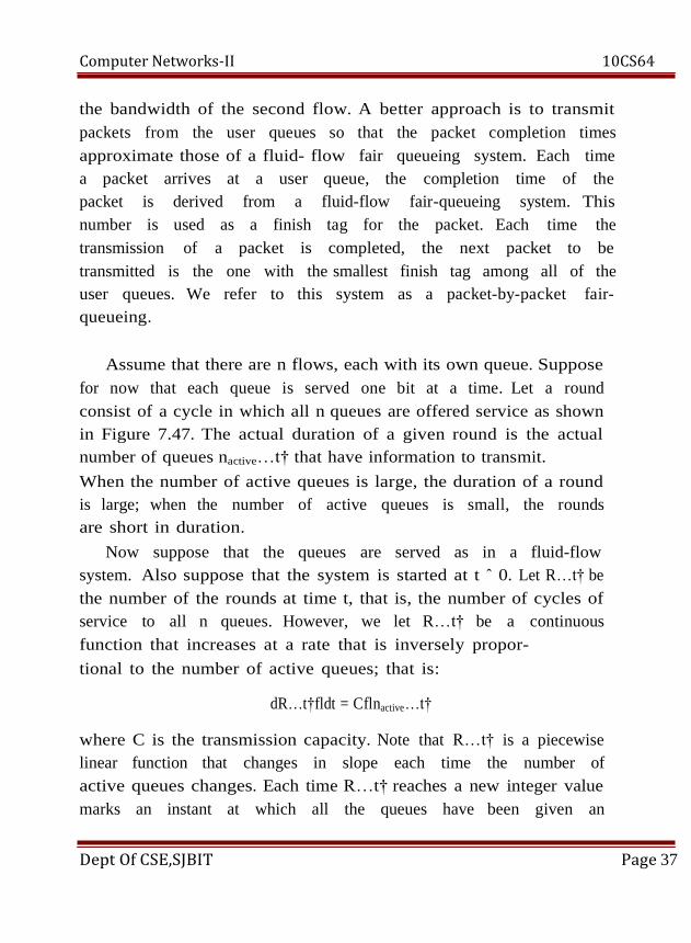
Assume that there are n flows, each with its own queue. Suppose
for now that each queue is served one bit at a time. Let a round
consist of a cycle in which all n queues are offered service as shown
in Figure 7.47. The actual duration of a given round is the actual
number of queues nactive…t† that have information to transmit.
When the number of active queues is large, the duration of a round
is large; when the number of active queues is small, the rounds
are short in duration.
Now suppose that the queues are served as in a fluid-flow
system. Also suppose that the system is started at t ˆ 0. Let R…t† be
the number of the rounds at time t, that is, the number of cycles of
service to all n queues. However, we let R…t† be a continuous
function that increases at a rate that is inversely propor-
tional to the number of active queues; that is:
dR…t†fldt = Cflnactive…t†
where C is the transmission capacity. Note that R…t† is a piecewise
linear function that changes in slope each time the number of
active queues changes. Each time R…t† reaches a new integer value
marks an instant at which all the queues have been given an
Dept Of CSE,SJBIT Page 37

Computer Networks-II 10CS64
equal number of opportunities to transmit a bit.
k Let us see how we can calculate the finish tags to approximate
fluid-flow fair queueing. Suppose
arrives at an empty queue at time ti
has length P…i; k†. This packet will complete its transmission when
P…i; k† rounds have elapsed, one round for each bit in the
packet. Therefore, the packet completion time will be the value
of time t
when the R…t† reaches the value:
F…i; k† ˆ R…ti † +P…i; k†
We will use F…i; k† as the finish tag of the packet. On the other
hand, if the kth packet from the ith flow arrives at a nonempty
queue, then the packet will have a finish tag F…i; k† equal to the
finish tag of the previous packet in its queue
F…i; k 1† plus its own packet length P…i; k†; that is:
F…i; k† ˆ F…i; k 1† + P…i; k†
The two preceding equations can be combined into the
1†; R…ti †g + P…i; k† for fair queueing:
FIGURE 1 .47 Computing the finishing time in packet- by-packet fair queueing and
weighted fair queueing
R(t) grows at rate inversely
proportional to nactive(t)
Dept Of CSE,SJBIT Page 38
the kth packet from flow i
and suppose that the packet
k
Generalize so R(t) is continuous, not discrete
following compact
equation:
F…i; k† = maxfF …i; k
Rounds
k

Computer Networks-II 10CS64
We reiterate: The actual packet completion time for the kth
packet in flow I in a fluid-flow fair-queueing system is the time t
when R…t† reaches the value F…i; k†. The relation between the actual
completion time and the finish tag is not straightforward because
the time required to transmit each bit varies according to the
number of active queues.
As an example, suppose that at time t 0 queue 1 has one packet
of length one unit and queue 2 has one packet of length two units.
A fluid-flow system services each queue at rate 1/2 as long as
both queues remain nonempty. As shown in Figure 1.48, queue 1
empties at time t = 2. Thereafter queue 2 is served at rate 1 until it
empties at time t = 3. In the packet-by-packet fair-queueing system,
the finish tag of the packet of queue 1 is F…1; 1† = R…0† + 1 = 1. The
finish tag of the packet from queue 2 is F…2; 1† = R…0† + 2 = 2. Since
the finish tag of the packet of queue 1 is smaller than the finish tag
of queue 2, the system will service queue 1 first. Thus the packet of
queue 1 completes its transmissions at time t = 1 and the packet of
queue 2 completes its transmissions at t = 3.
Dept Of CSE,SJBIT Page 39
Computer Networks-II 10CS64
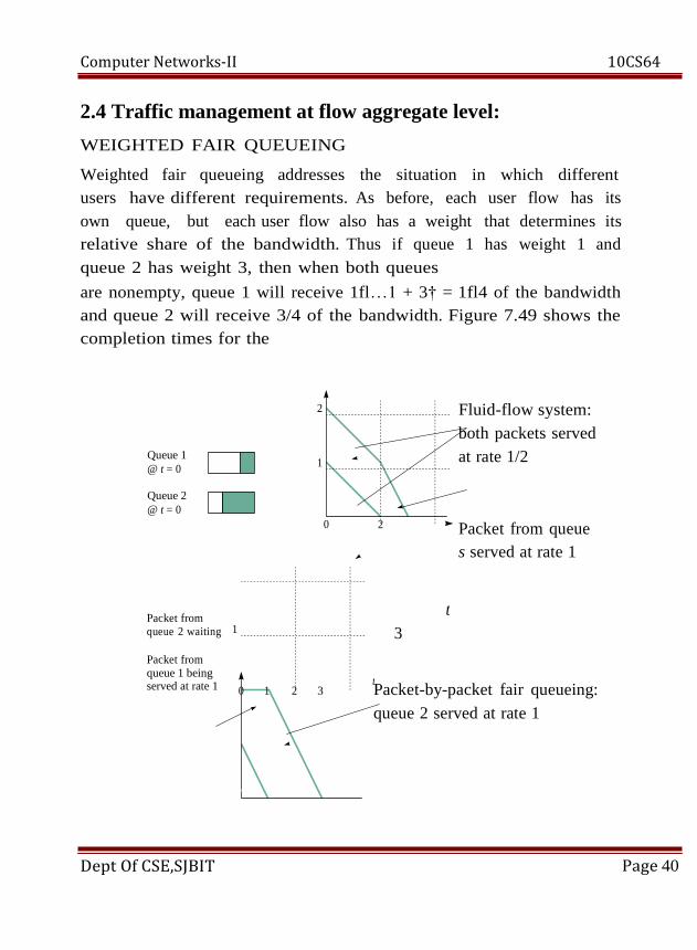
2.4 Traffic management at flow aggregate level:
WEIGHTED FAIR QUEUEING
Weighted fair queueing addresses the situation in which different
users have different requirements. As before, each user flow has its
own queue, but each user flow also has a weight that determines its
relative share of the bandwidth. Thus if queue 1 has weight 1 and
queue 2 has weight 3, then when both queues
are nonempty, queue 1 will receive 1fl…1 + 3† = 1fl4 of the bandwidth
and queue 2 will receive 3/4 of the bandwidth. Figure 7.49 shows the
completion times for the
Queue 1
@ t = 0
Queue 2
@ t = 0
Packet from queue 2 waiting
Packet from queue 1 being served at rate 1
Dept Of CSE,SJBIT
2
1
0
1
0 1 2 3
2
t
3
Packet-by-packet fair queueing:
queue 2 served at rate 1
Page 40
t
Fluid-flow system:
both packets served
at rate 1/2
Packet from queue
s served at rate 1
Computer Networks-II 10CS64
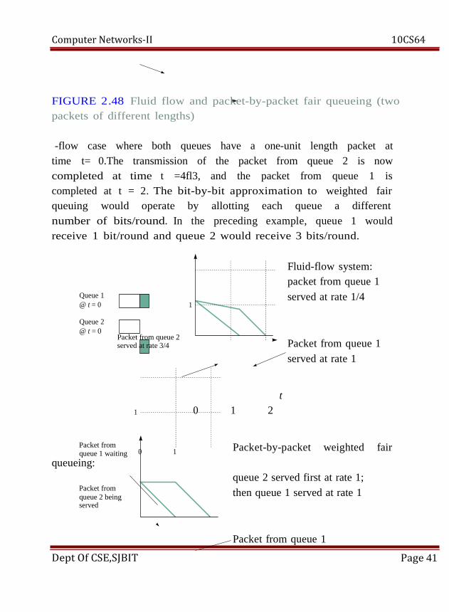
FIGURE 2.48 Fluid flow and packet-by-packet fair queueing (two
packets of different lengths)
-flow case where both queues have a one-unit length packet at
time t= 0.The transmission of the packet from queue 2 is now
completed at time t =4fl3, and the packet from queue 1 is
completed at t = 2. The bit-by-bit approximation to weighted fair
queuing would operate by allotting each queue a different
number of bits/round. In the preceding example, queue 1 would
receive 1 bit/round and queue 2 would receive 3 bits/round.
Fluid-flow system:
packet from queue 1
served at rate 1/4
Packet from queue 1
served at rate 1
t
0 1 2
Packet-by-packet weighted fair
queue 2 served first at rate 1;
then queue 1 served at rate 1
Packet from queue 1
Page 41
0 1
1
Packet from queue 2 served at rate 3/4
1
Queue 1
@ t = 0
Queue 2
@ t = 0
Packet from queue 1 waiting
queueing:
Packet from
queue 2 being served
Dept Of CSE,SJBIT

Computer Networks-II 10CS64
FIGURE2.49 Fluid flow and packetized, weighted fair
queueing
Weighted fair-queueing systems are a means for providing QoS
guarantees. Suppose a given user flow has weight wi and suppose
that the sum of the weights of all the user flows is W . In the worst
case when all the user queues are non- empty, the given user flow
will receive a fraction wiflW of the bandwidth C.
When other user queues are empty, the given user flow will
receive a greater
share.
Dept Of CSE,SJBIT Page 42
Computer Networks-II 10CS64
UNIT – 3
TCP/IP-1: TCP/IP architecture, The Internet Protocol, IPv6, UDP.
Dept Of CSE,SJBIT Page 43

Computer Networks-II 10CS64
UNIT – 3
TCP/IP-1:
The Internet Protocol (IP) enables communications across a
vast and heterogeneous collection of networks that are based on
different technologies. Any host computer that is connected to the
Internet can communicate with any other computer that is also
connected to the Internet. The Internet therefore offers ubiquitous
connectivity and the economies of scale that result from large
deployment.
The Internet offers two basic communication services that
operate on top of IP: Transmission control protocol (TCP) reliable
stream service and user datagram protocol (UDP) datagram
service. Any application layer protocol that operates on top of
either TCP or UDP automatically operates across the Internet.
Therefore the Internet provides a ubiquitous platform for the
deployment of network-based services.
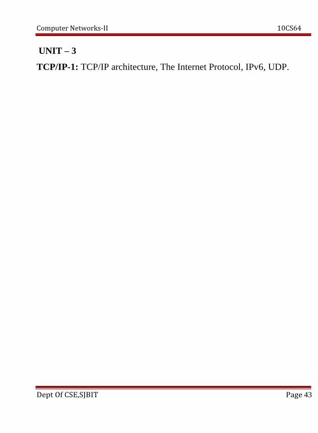
3.1 THE TCP/IP ARCHITECTURE
The TCP/IP protocol suite usually refers not only to the two
most well-known protocols called the Transmission Control
Protocol (TCP) and the Internet Protocol (IP) but also to other
related protocols such as the User Datagram Protocol (UDP), the
Internet Control Message Protocol (ICMP) and the basic
applications such as HTTP, TELNET, and FTP. The basic
structure of the TCP/IP protocol suite is shown in Figure 3 .1.
Application layer protocols such as SNMP and DNS send their
messages using UDP. The PDUs exchanged by the peer TCP
protocols are called TCP segments or segments, while those
Dept Of CSE,SJBIT Page 44
Computer Networks-II 10CS64
exchanged by UDP protocols are called UDP datagrams or
datagrams. IP multiplexes TCP segments and UDP datagrams and
performs fragmentation, if necessary, among other tasks to be
discussed below. The protocol data units exchanged by IP
protocols are called IP packets or packets.1 IP packets are sent to
the network interface for delivery across the physical network. At
the receiver, packets passed up by the network interface are
demultiplexed to the appropriate protocol (IP, ARP, or RARP).
The receiving IP entity needs to determine whether a packet has
to be sent to TCP or UDP. Finally, TCP (UDP) sends each
segment (datagram) to the appropriate application based on the
port number. The physical network can be implemented by a
variety of technologies such as Ethernet, token ring, ATM, PPP
over various transmission systems, and others.
FIGURE 3.1 TCP/IP
protocol suite
RARP
Physical
Dept Of CSE,SJBIT Page 45
Application
UDP
ARP
Application
TCP
ICMP IP
Computer Networks-II 10CS64
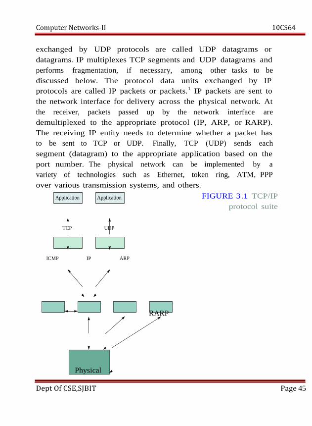
The PDU of a given layer is encapsulated in a PDU of the
layer below as shown in Figure 8.2. In this figure an HTTP GET
command is passed to the TCP layer, which encapsulates the
message into a TCP segment. The segment header contains an
ephemeral port number for the client process and the well-known
port 80 for the HTTP server process. The TCP segment in turn is
passed to the IP layer where it is encapsulated in an IP packet. The
IP packet header contains an IP network address for the sender and
an IP network address for the destination. IP network addresses are
said to be logical because they are defined in terms of the logical
topology of the routers and end systems. The IP packet is then
passed through the network interface and encapsulated into a PDU
of the underlying network. In Figure 2.2 the IP packet is
encapsulated into an Ethernet LAN frame. The frame header
contains physical addresses that identify the physical endpoints for
the sender and the receiver. The logical IP addresses need to be
converted into specific physical addresses to carry out the transfer
of bits from one device to the other. This conversion is done by an
address resolution protocol.
Each host in the Internet is identified by a globally unique IP
address. An IP address is divided into two parts: a network ID and
a host ID. The network ID
Dept Of CSE,SJBIT Page 46

Computer Networks-II 10CS64
Header contains
source and destination
port numbers
IP header
Header contains
source and destination
IP addresses;
transport protocol type
Header contains Ethernet
source and destinhetaiden
physical addresses;
network protocol type
FIGURE 3.2 Encapsulation of PDUs in TCP/IP and
addressing information in
the headers
Dept Of CSE,SJBIT Page 47
a or
Computer Networks-II 10CS64
must be obtained from an organization authorized to issue IP
addresses. The Internet layer provides for the transfer of
information across multiple networks through the use of routers,
as shown in Figure 2.3. The Internet layer provides a single
service, namely, best-effort connectionless packet transfer. IP
packets are exchanged between routers without a connection
setup; they are routed indepen- dently, and may traverse different
paths. The gateways that interconnect the intermediate networks
may discard packets when they encounter congestion. The
responsibility for recovery from these losses is passed on to the
transport layer.
The network interface layer is particularly concerned with the
protocols that are used to access the intermediate networks. At
each gateway the network protocol is used to encapsulate the IP
packet into a packet or frame of the underlying network or link.
The IP packet is recovered at the exit router of the given
network. This router must determine the next hop in the route to
the destination and then encapsulate the IP packet or frame of the
type of the next network or link. This approach provides a clear
separation of the Internet layer from the technology-dependent
network interface layer. This approach also allows the Internet
layer to provide a data transfer service that is transparent in the
sense of not depending on the details of the underlying networks.
Different network technologies impose different limits on the size
of the blocks that they can handle. IP must accommodate the
maximum transmission unit of an under-
lying network or link by implementing segmentation and
reassembly as needed.
To enhance the scalability of the routing algorithms and to
control the size of the routing tables, additional levels of
hierarchy are introduced in the IP
Dept Of CSE,SJBIT Page 48
Computer Networks-II 10CS64
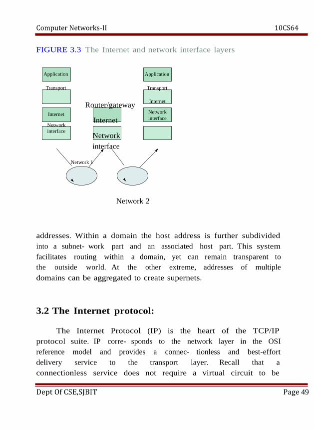
FIGURE 3.3 The Internet and network interface layers
Application
Transport
Internet
Network interface
Network 1
Network 2
addresses. Within a domain the host address is further subdivided
into a subnet- work part and an associated host part. This
facilitates routing within a domain, yet can remain transparent to
the outside world. At the other extreme, addresses of multiple
domains can be aggregated to create supernets.
3.2 The Internet protocol:
The Internet Protocol (IP) is the heart of the TCP/IP
protocol suite. IP corre- sponds to the network layer in the OSI
reference model and provides a connec- tionless and best-effort
delivery service to the transport layer. Recall that a
connectionless service does not require a virtual circuit to be
Dept Of CSE,SJBIT Page 49
Application
Transport
Internet
Network
interface
Router/gateway
Internet
Network
interface
system

Computer Networks-II 10CS64
established before data transfer can begin. The term best-effort
indicates that IP will try its best to forward packets to the
destination, but does not guarantee that a packet will be delivered
to the destination. The term is also used to indicate that IP does
not make any guarantee on the QoS.2 An application requiring high
reliability must implement the reliability function within a higher-
layer protocol.
IP Packet
To understand the service provided by the IP entity, it is useful to
examine the IP packet format, which contains a header part and a
data part. The format of the IP header is shown in Figure 3.4.
The header has a fixed-length component of 20 bytes plus a
variable-length component consisting of options that can be up to
40 bytes. IP packets are
0 4 8 16 19 24
31
Version IHL Type of service Total length
Identification Flags Fragment offset
Time to live Protocol Header checksum
Source IP address
Destination IP address
Options Padding
FIGURE 3.4 IP version 4 headers
Dept Of CSE,SJBIT Page 50

Computer Networks-II 10CS64
transmitted according to network byte order: bits 0±7 first, then
bits 8±15, then bits 16±23, and finally bits 24±31 for each row. The
meaning of each field in the header follows.
Version: The version field indicates the version number used by
the IP packet so that revisions can be distinguished from each
other. The current IP version is 4. Version 5 is used for a real-
time stream protocol called ST2, and version 6 is used for the
new generation IP know as IPng or IPv6 (to be discussed in the
following section).
Internet header length: The Internet header length (IHL)
specifies the length of the header in 32-bit words. If no options
are present, IHL will have a value of 5. The length of the options
field can be determined from IHL.
Type of service: The type of service (TOS) field specifies the
priority of the packet based on delay, throughput, reliability, and
cost requirements. Three bits are assigned for priority levels
(called ``precedence'') and four bits for the specific requirement
(i.e., delay, throughput, reliability, and cost). For example, if a
packet needs to be delivered to the destination as soon as
possible, the transmitting IP module can set the delay bit to one
and use a high-priority level. In practice most routers ignore this
field.
Recent work in the Differentiated Service Working Group
of IETF tries to redefine the TOS field in order to support other
services that are better than the basic best effort.
Total length: The total length specifies the number of bytes of
the IP packet including header and data. With 16 bits assigned to
this field, the max- imum packet length is 65,535 bytes. In
practice the maximum possible length is very rarely used, since
most physical networks have their own length limitation. For
example, Ethernet limits the payload length to 1500 bytes.
Dept Of CSE,SJBIT Page51
Computer Networks-II 10CS64
Identification, flags, and fragment offset: These fields are used
for fragmentation and reassembly and are discussed below.
Time to live: The time-to-live (TTL) field is defined to indicate the
amount of time in seconds the packet is allowed to remain in the
network. However, most routers interpret this field to indicate the
number of hops the packet is allowed to traverse in the network.
Initially, the source host sets this field to some value. Each router
decrements this value by one. If the value reaches zero before the
packet reaches the destination, the router discards the packet and
sends an error message back to the source. With either
interpretation, this field prevents packets from wandering aimlessly
in the Internet.
Protocol: The protocol field specifies the protocol that is to
receive the IP data at the destination host. Examples of the
protocols include TCP (pro- tocol fl 6), UDP (protocol fl 17), and
ICMP (protocol fl 1). Header checksum: The header checksum field
verifies the integrity of the header of the IP packet. The data part
is not verified and is left to upper-layer protocols. If the
verification process fails, the packet is simply discarded. To compute
the header checksum, the sender first sets the header checksum
field to 0 and then applies the Internet checksum algorithm
discussed in Chapter 3. Note that when a router decrements the TTL
field, the router must also recompute the header checksum field.
Source IP address and destination IP address: These fields
contain the addresses of the source and destination hosts. The format
of the IP address is discussed below.
Options: The options field, which is of variable length, allows
the packet to request special features such as security level, route to
be taken by the packet, and timestamp at each router. The options
field is rarely used. Router alert is a new option introduced to
alert routers to look inside the IP packet. The option is intended
for new protocols that require rela- tively complex processing in
Dept Of CSE,SJBIT Page 52

Computer Networks-II 10CS64
routers along the path [RFC 2113].
Padding: This field is used to make the header a multiple of 32-
bit words.
When an IP packet is passed to the router by a network
interface, the following processing takes place. First the header
checksum is computed and the fields in the header are checked to
see if they contain valid values. Next IP fields that need to be
changed are updated. For example, the TTL and header checksum
fields always require updating. The router then identifies the next
loop for the IP packet by consulting its routing tables. The IP
packet is then for- warded along the next loop.
3.3 IPv6
IP version 4 has played a central role in the
internetworking environment for many years. It has proved
flexible enough to work on many different networking
technologies. However, it has become a victim of its own
success Ðexplosive growth! In the early days of the Internet, people
using it were typically researchers and scientists working in
academia, high-tech companies, and research laboratories, mainly
for the purpose of exchanging scientific results through e- mails.
In the 1990s the World Wide Web and personal computers shifted
the user of the Internet to the general public. This change has
created heavy demands for new IP addresses, and the 32 bits of
the current IP addresses will be exhausted sooner or later.
In the early1990s the Internet Engineering Task Force
(IETF) began to work on the successor of IP version 4 that would
solve the address exhaustion problem and other scalability
problems. After several proposals were investigated, the new IP
version was recommended in late 1994. The new version is called
Dept Of CSE,SJBIT Page 53
Computer Networks-II 10CS64
IPv6 for IP version 6 (also called IP next generation or IPng).
IPv6 was designed to interoperate with IPv4 since it would likely
take many years to complete the transition from version 4 to
version 6. Thus IPv6 should retain the most basic service
provided by IPv4Ða connectionless delivery service. On the other
hand, IPv6 should also change the IPv4 functions that do not
work well and support new emerging applications such as real-time
video conferencing, etc. Some of the changes from IPv4 to IPv6
include Longer address fields: The length of address field is
extended from 32 bits to128 bits. The address structure also
provides more levels of hierarchy.
Theoretically, the address space can support up to 3:4 1038
hosts. Simplified header format: The header format of IPv6 is
simpler than that of IPv4. Some of the header fields in IPv4 such as
checksum, IHL, identifica- tion, flags, and fragment offset do not
appear in the IPv6 header.
Flexible support for options: The options in IPv6 appear in
optional extension headers that are encoded in a more efficient and
flexible fashion than they were in IPv4.
Flow label capability: IPv6 adds a ``flow label'' to identify a
certain packet ``flow'' that requires a certain QoS. Security: IPv6
supports built-in authentication and confidentiality. Large packets:
IPv6 supports payloads that are longer than 64 K bytes, called
jumbo payloads. Fragmentation at source only: Routers are not
allowed to fragment packets. If a packet needs to be fragmented, it
must be done at the source. No checksum field: The checksum field
has been removed to reduce packet processing time in a router.
Packets carried by the physical network such as Ethernet, token
ring, X.25, or ATM are typically already checked. Furthermore,
higher-layer protocols such as TCP and UDP also perform their
own verification. Thus removing the checksum field probably would
not introduce a serious problem in most situations.
Dept Of CSE,SJBIT Page 54
Computer Networks-II 10CS64
Header Format
The IPv6 header consists of a required basic header and optional
extension headers. The format of the basic header is shown in
Figure 8.10. The packet should be transmitted in network byte
order. The description of each field in the basic header follows.
Version: The version field specifies the version number of the
protocol and should be set to 6 for IPv6. The location and length of
the version field stays unchanged so that the protocol software can
recognize the version of the packet quickly. Traffic class: The traffic
class field specifies the traffic class or priority of the packet. The
traffic class field is intended to support differentiated service.
Flow label: The flow label field can be to identify the QoS
requested by the packet. In the standard, a flow is defined as ``a
sequence of packets sent from a particular source to a particular
(unicast or multicast) destination for which the source desires
special handling by the intervening routers.''
An example of an application that may use a flow label is a
packet video system that requires its packets to be delivered to the
destination within a certain time constraint. Routers that see these
packets will have to process them according to their request.
Hosts that do not support flows are required to set this field to
0.
Payload length: The payload length indicates the length of the
data (excluding header). With 16 bits allocated to this field, the
payload length is limited to 65,535 bytes. As we explain below, it
is possible to send larger payloads by using the option in the
extension header. Next header: The next header field identifies the
type of the extension header that follows the basic header. The
extension header is similar to the options field in IPv4 but is
more flexible and efficient. Extension headers are further discussed
below.
Dept Of CSE,SJBIT Page 55
Computer Networks-II 10CS64
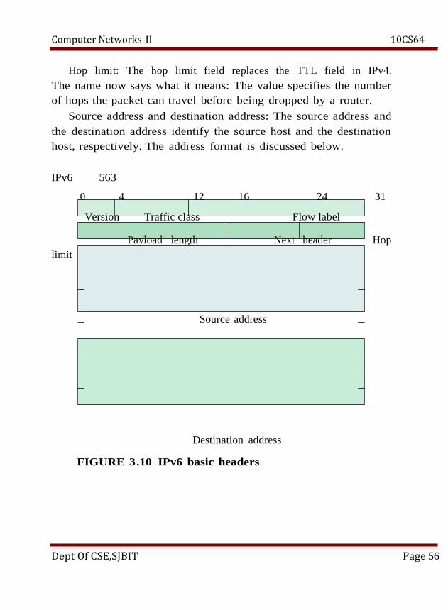
Hop limit: The hop limit field replaces the TTL field in IPv4.
The name now says what it means: The value specifies the number
of hops the packet can travel before being dropped by a router.
Source address and destination address: The source address and
the destination address identify the source host and the destination
host, respectively. The address format is discussed below.
IPv6 563
0 4 12 16 24 31
Version Traffic class Flow label
Payload length Next header Hop
limit
Source address
Destination address
FIGURE 3.10 IPv6 basic headers
Dept Of CSE,SJBIT Page 56
Computer Networks-II 10CS64
3.4 User datagram protocol:
Two transport layer protocols, TCP and UDP, build on the
best-effort service provided by IP to support a wide range of
applications. In this section we discuss the details of UDP.
The User Datagram Protocol (UDP) is an unreliable,
connectionless trans- port layer protocol. It is a very simple
protocol that provides only two additional services beyond IP:
demultiplexing and error checking on data. Recall that IP knows
how to deliver packets to a host, but does not know how to deliver
them to the specific application in the host. UDP adds a mechanism
that distinguishes among multiple applications in the host. Recall
also that IP checks only the integrity of its header. UDP can
optionally check the integrity of the entire UDP datagram.
Applications that use UDP include Trivial File Transfer
Protocol, DNS, SNMP, and Real-Time Protocol (RTP).
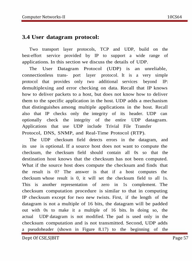
The UDP checksum field detects errors in the datagram, and
its use is optional. If a source host does not want to compute the
checksum, the checksum field should contain all 0s so that the
destination host knows that the checksum has not been computed.
What if the source host does compute the checksum and finds that
the result is 0? The answer is that if a host computes the
checksum whose result is 0, it will set the checksum field to all 1s.
This is another representation of zero in 1s complement. The
checksum computation procedure is similar to that in computing
IP checksum except for two new twists. First, if the length of the
datagram is not a multiple of 16 bits, the datagram will be padded
out with 0s to make it a multiple of 16 bits. In doing so, the
actual UDP datagram is not modified. The pad is used only in the
checksum computation and is not transmitted. Second, UDP adds
a pseudoheader (shown in Figure 8.17) to the beginning of the
Dept Of CSE,SJBIT Page 57

Computer Networks-II 10CS64
datagram when performing the checksum computation. The
pseudoheader is also created by the source and destination hosts
only during the checksum computation and is not transmitted. The
pseudoheader is to ensure
0 16 31
Source port Destination port
UDP length UDP checksum
Data
0 8 16 31
Source IP address
Destination IP address
Protocol = 17 UDP length
0 0 0 0 0 0 0 0
FIGURE 3.17 UDP pseudoheader
that the datagram has indeed reached the correct destination
host and port. Finally, if a datagram is found to be corrupted, it is
simply discarded and the source UDP entity is not notified.
Dept Of CSE,SJBIT Page 58

Computer Networks-II 10CS64
UNIT – 4
TCP/IP-2: TCP, Internet Routing Protocols, Multicast Routing, DHCP,
NAT and Mobile IP.
Dept Of CSE,SJBIT Page 59
Computer Networks-II 10CS64
UNIT – 4
TCP/IP-2:
4.1 Transmission control protocol:
TCP and IP are the workhorses in the Internet. In this
section we first discuss how TCP provides reliable, connection-
oriented stream service over IP. To do so, TCP implements a
version of Selective Repeat ARQ. In addition, TCP implements
congestion control through an algorithm that identifies
congestion through packet loss and that controls the rate at which
information enters the network through a congestion window.
TCP Reliable Stream Service
The Transmission Control Protocol (TCP) provides a logical
full-duplex (two- way) connection between two application layer
processes across a datagram network. TCP provides these
application processes with a connection-oriented,reliable, in-
sequence, byte-stream service. TCP also provides flow control that
allows receivers to control the rate at which the sender transmits
information so that buffers do not overflow. TCP can also support
multiple application processes in the same end system.
TCP does not preserve message boundaries and treats the data
it gets from the application layer as a byte stream. Thus when a
source sends a 1000-byte message in a single chunk (one write),
the destination may receive the message in two chunks of 500 bytes
each (two reads), in three chunks of 400 bytes, 300 bytes and 300
bytes (three reads), or in any other combination. In other words,
Dept Of CSE,SJBIT Page 60

Computer Networks-II 10CS64
TCP may split or combine the application information in the way it
finds most appropriate for the underlying network.
TCP Operation
We now consider the adaptation functions that TCP uses
to provide a connection-oriented, reliable, stream service. We are
interested in delivering the user information so that it is error
free, without duplication, and in the same order that it was
produced by the sender. We assume that the user information
consists of a stream of bytes as shown in Figure 8.18. For
example, in the transfer of a long file the sender is viewed as
inserting a byte stream into the transmitter's send buffer. The task of
TCP is to ensure the transfer of the byte stream to the receiver and
the orderly delivery of the stream to the destination application.
TCP was designed to deliver a connection-oriented service in an
internet environment, which itself offers connectionless packet
transfer service, so different packets can traverse a different path
from the same source to the same destination and can therefore
arrive out of order. Therefore, in the internet old messages from
previous connections may arrive at a receiver, thus potentially
complicating the task of eliminating duplicate messages. TCP
deals with this problem by using long (32 bit) sequence numbers
and by establishing randomly selected initial sequence numbers
during connection setup. At any given time the receiver is accepting
sequence numbers from a much smaller window, so the
likelihood of accepting a very old message is very low. In addition,
TCP enforces a time-out period at the end of each connection to
allow the network to clear old segments from the network.
TCP uses a sliding-window mechanism, as shown in Figure
4.19. The send window contains three pointers: Slast points to the
oldest byte that has not yet been acknowledged.
Dept Of CSE,SJBIT Page61
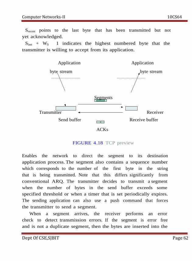
Computer Networks-II 10CS64
Srecent points to the last byte that has been transmitted but not
yet acknowledged.
Slast + WS 1 indicates the highest numbered byte that the
transmitter is willing to accept from its application.
Application Application
byte stream byte stream
Segments
Transmitter Receiver
Send buffer Receive buffer
ACKs
FIGURE 4.18 TCP preview
Enables the network to direct the segment to its destination
application process. The segment also contains a sequence number
which corresponds to the number of the first byte in the string
that is being transmitted. Note that this differs significantly from
conventional ARQ. The transmitter decides to transmit a segment
when the number of bytes in the send buffer exceeds some
specified threshold or when a timer that is set periodically expires.
The sending application can also use a push command that forces
the transmitter to send a segment.
When a segment arrives, the receiver performs an error
check to detect transmission errors. If the segment is error free
and is not a duplicate segment, then the bytes are inserted into the
Dept Of CSE,SJBIT Page 62

Computer Networks-II 10CS64
appropriate locations in the receive buffer if the bytes fall within
the receive window. Note that the receiver will accept out-of-order
but error-free segments. If the received segment contains the byte
corresponding to Rnext, then the Rnext pointer is moved forward to
the location of the next byte that has not yet been received. An
acknowledgment with the sequence number Rnext is sent in a
segment that is transmitted in the reverse direction. Rnext
acknowledges the correct receipt of all bytes up to Rnext 1. This
acknowledgment, when received by the transmitter, enables the
transmitter to update its parameter Slast to Rnext, thus moving the
send window forward. Later in the section we give an example
of data transfer in TCP.
TCP separates the flow control function from the
acknowledgment function.The flow control function is
implemented through an advertised window field in the segment
header. Segments that travel in the reverse direction contain the
advertised window size that informs the transmitter of the
number of buffers currently available at the receiver. The
advertised window size is given by
WA ˆ WR …Rnew Rlast†
The transmitter is obliged to keep the number of outstanding
bytes below the advertised window size, that is
Srecent Slast WA
To see how the flow control takes effect, suppose that the
application at the receiver's side stops reading the bytes from the
buffer. Then Rnew will increase while Rlast remains fixed, thus
leading to a smaller advertised window size.
Eventually the receive window will be exhausted when Rnew Rlast
ˆ WR, and the advertised window size will be zero. This condition
will cause the transmitter to stop sending. The transmitter can
continue accepting bytes from its application until its buffer
Dept Of CSE,SJBIT Page 63

Computer Networks-II 10CS64
contains WS bytes. At this point the transmitter blocks its
application from inserting any more bytes into the buffer.
Finally, we consider the retransmission procedure that is used
in TCP. The transmitter sets a timer each time a segment is
transmitted. If the timer expires before any of the bytes in the
segment are acknowledged, then the segment is retransmitted.
TCP Protocol
We now discuss the structure of TCP segments and the setting up
of a TCP connection, the data transfer phase, and the closing of
the connection. Detailed information about TCP can be found in
RFC 793 and RFC 1122.
TCP SEGMENT
Figure 8.20 shows the format of the TCP segment. The header
consists of a 20 The description of each field in the TCP segment
is given below. The term sender refers to the host that sends the
segment, and receiver refers to the host that receives the segment.
Source port and destination port: The source and destination
ports identify the sending and receiving applications, respectively.
Recall from section 2.3.1 that the pair of ports and IP addresses
identify a process-to-process connection. byte fixed part plus a
variable-size options field.
Dept Of CSE,SJBIT Page 64

Computer Networks-II 10CS64
0 4
Source port
Header
length
Reserved
Checksum
Options
Data
FIGURE 4.20
Dept Of CSE,SJBIT
24 31
Destination port
Window size
Urgent pointer
Padding
16
Sequence number
Acknowledgment number
10
P R S S H T
S F Y I N N
A C K
U R G
TCP segment
Page 65

Computer Networks-II 10CS64
Sequence number: The 32-bit sequence number field identifies
the position of the first data byte of this segment in the sender's
byte stream during data transfer (when SYN bit is not set). The
sequence number wraps back to 0 after 232 1. Note that TCP
identifies the sequence number for each byte (rather than for each
segment). For example, if the value of the sequence number is 100
and the data area contains five bytes, then the next time this
TCP module sends a segment, the sequence number will be
105. If the SYN bit is set to 1 (during connection establishment),
the sequence number indicates the initial sequence number (ISN)
to be used in the sender's byte stream. The sequence number of
the first byte of data for this byte stream will be ISN+1. It is
important to note that a TCP connection is full duplex so that each
end point independently maintains its own sequence number.
Acknowledgment number: This field identifies the sequence
number of the next data byte that the sender expects to receive if
the ACK bit is set. This field also indicates that the sender has
successfully received all data up to but not including this value. If
the ACK bit is not set (during connection establishment), this field
is meaningless. Once a connection is established, the ACK bit
must be set.
Header length: This field specifies the length of the TCP
header in 32-bit words. This information allows the receiver to
know the beginning of the data area because the options field is
variable length.
Reserved: As the name implies, this field is reserved for future
use and must be set to 0.
URG: If this bit is set, the urgent pointer is valid (discussed
shortly).
ACK: If this bit is set, the acknowledgment number is valid.
PSH: When this bit is set, it tells the receiving TCP module to
Dept Of CSE,SJBIT Page 66

Computer Networks-II 10CS64
pass the data to the application immediately. Otherwise, the
receiving TCP module may choose to buffer the segment until
enough data accumulates in its buffer.
RST: When this bit is set, it tells the receiving TCP module
to abort the connection because of some abnormal condition.
SYN: This bit requests a connection (discussed later).
FIN: When this bit is set, it tells the receiver that the sender
does not have any more data to send. The sender can still
receive data from the other direction until it receives a segment
with the FIN bit set.
Window size: The window size field specifies the number of bytes
the sender is willing to accept. This field can be used to control
the flow of data and congestion.
Checksum: This field detects errors on the TCP segment. The
procedure is discussed below.
Urgent pointer: When the URG bit is set, the value in the
urgent pointer field added to that in the sequence number field
points to the last byte of the ``urgent data'' (data that needs
immediate delivery). However, the first byte of the urgent data
is never explicitly defined. Because the receiver's TCP module
passes data to the application in sequence, any data in the
receiver's buffer up to the last byte of the urgent data may be
considered urgent.
Options: The options field may be used to provide other
functions that are not covered by the header. If the length of the
options field is not a multiple of 32 bits, extra padding bits will be
added. The most important option is used by the sender to
indicate the maximum segment size (MSS) it can accept. This
option is specified during connection setup. Two other options
that are negotiated during connection setup are intended to deal
with situations that involve large delay-bandwidth products. The
Dept Of CSE,SJBIT Page 67

Computer Networks-II 10CS64
window scale option allows the use of a larger advertised window
size. The window can be scaled upward by a factor of up to 214.
Normally the maximum window size is 216 1 ˆ 65,535. With
scaling the maximum advertised window size is 65,535 214 fl
1,073,725,440 bytes. The timestamp option is intended for high-
speed connections where the sequence numbers may wrap
around during the lifetime of the connection. The timestamp
option allows the sender to include a timestamp in every segment.
This timestamp can also be used in the RTT calculation.
TCP CHECKSUM
The purpose of the TCP checksum field is to detect errors. The
checksum com putation procedure is similar to that used to
compute an IP checksum (discussed in Chapter 3) except for two
features. First, if the length of the segment is not a multiple of 16
bits, the segment will be padded with zeros to make it a multiple
of 16 bits. In doing so, the TCP length field is not modified.
Second, a pseudoheader (shown in Figure 8.21) is added to the
beginning of the segment when performing the checksum
computation.
0 8 16
31
Source IP address
Destination IP address
0 0 0 0 0 0 0 0 Protocol fl 6 TCP segment
length
FIGURE 4.21 TCP pseudoheader
Dept Of CSE,SJBIT Page 68

Computer Networks-II 10CS64
CONNECTION ESTABLISHMENT
Before any host can send data, a connection must be established.
TCP establishes
the connection using a three-way handshake procedure shown in
Figure 8.22. The
handshakes are described in the following steps:
1. Host A sends a connection request to host B by setting the
SYN bit. Host A
also registers its initial sequence number to use (Seq_no fl x).
2. Host B acknowledges the request by setting the ACK bit and
indicating the next data byte to receive (Ack_no fl x + 1). The
``plus one'' is needed because the SYN bit consumes one
sequence number. At the same time, host B also sends a request
by setting the SYN bit and registering its initial sequence number
to use (Seq_no fl y).
3. Host A acknowledges the request from B by setting the ACK
bit and con firming the next data byte to receive (Ack_no fl y
+ 1). Note that the sequence number is set to x + 1. On receipt at
B the connection is established.
If during a connection establishment phase, one of the hosts
decides to refuse a connection request, it will send a reset segment
by setting the RST bit. Each SYN message can specify options
such as maximum segment size, window scal- ing, and timestamps.
Because TCP segments can be delayed, lost, and duplicated,
the initial sequence number should be different each time a host
requests a connection.
Dept Of CSE,SJBIT Page 69

Computer Networks-II 10CS64
TCP CONNECTION TERMINATION
TCP provides for a graceful close that involves the independent
termination of each direction of the connection. A termination is
initiated when an application tells TCP that it has no more data to
send. The TCP entity completes transmis- sion of its data and,
upon receiving acknowledgment from the receiver, issues a
segment with the FIN bit set. Upon receiving a FIN segment, a
TCP entity informs its application that the other entity has
terminated its transmission of data. For example, in Figure 8.27
the TCP entity in host A terminates its trans- mission first by
issuing a FIN segment. Host B sends an ACK segment to
acknowledge receipt of the FIN segment from A. Note that the
FIN segment uses one byte, so the ACK is 5087 in the example.
After B receives the FIN segment, the direction of the flow
from B to A is still open. In Figure 8.27 host B sends 150 bytes in
one segment, followed by a FIN segment. Host A then sends an
acknowledgment. The TCP in host A then enters the
TIME_WAIT state and starts the TIME_WAIT timer with an
initial value set to twice the maximum segment lifetime (2MSL).
Dept Of CSE,SJBIT Page 70
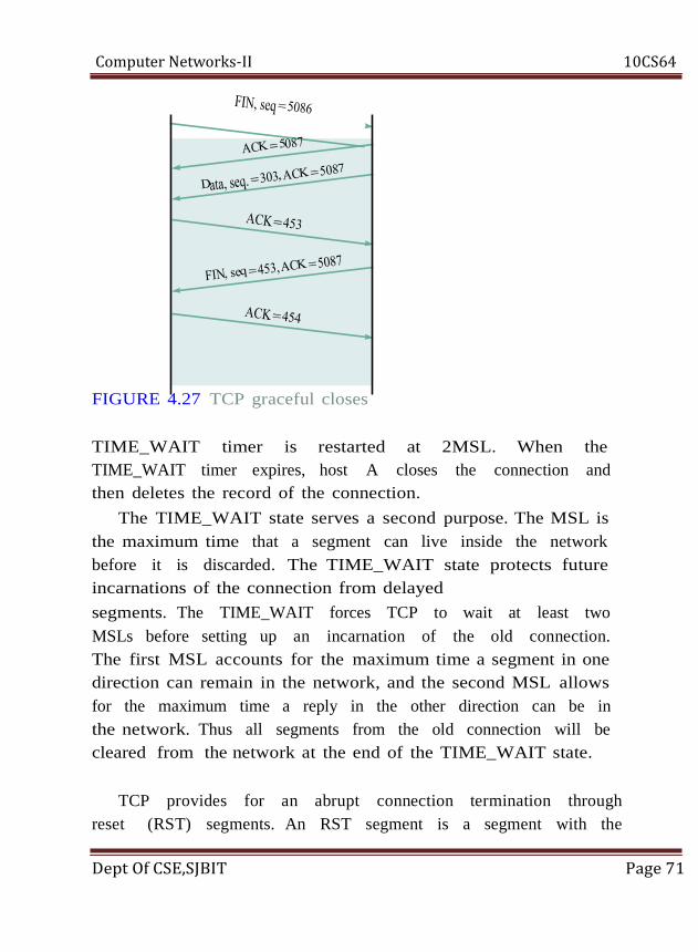
Computer Networks-II 10CS64
FIGURE 4.27 TCP graceful closes
TIME_WAIT timer is restarted at 2MSL. When the
TIME_WAIT timer expires, host A closes the connection and
then deletes the record of the connection.
The TIME_WAIT state serves a second purpose. The MSL is
the maximum time that a segment can live inside the network
before it is discarded. The TIME_WAIT state protects future
incarnations of the connection from delayed
segments. The TIME_WAIT forces TCP to wait at least two
MSLs before setting up an incarnation of the old connection.
The first MSL accounts for the maximum time a segment in one
direction can remain in the network, and the second MSL allows
for the maximum time a reply in the other direction can be in
the network. Thus all segments from the old connection will be
cleared from the network at the end of the TIME_WAIT state.
TCP provides for an abrupt connection termination through
reset (RST) segments. An RST segment is a segment with the
Dept Of CSE,SJBIT Page 71
Computer Networks-II 10CS64
RST bit set. If an application decides to terminate the connection
abruptly, it issues an ABORT command, which causes TCP to
discard any data that is queued for transmission and to send an
RST segment. The TCP that receives the RST segment then
notifies its application process that the connection has been
terminated.
Tcp state transition diagram:
A TCP connection goes through a series of states during its
lifetime. Figure 8.28 shows the state transition diagram. Each
state transition is indicated by an arrow, and the associated
label indicates associated events and actions. Connection
establishment begins in the CLOSED state and proceeds to
the ESTABLISHED state. Connection termination goes
from the ESTABLISHED state to the CLOSED state. The
normal transitions for a client are indicated by thick solid lines,
and the normal transitions for a server are denoted by dashed
lines. Thus when a client does an active open, it goes from the
CLOSED state, to SYN_SENT, and then to ESTABLISHED. The
server carry- ing out a passive open goes from the CLOSED state,
to LISTEN, SYN_RCVD, and then to ESTABLISHED.
The client normally initiates the termination of the
connection by sending a FIN. The associated state trajectory
goes from the ESTABLISHED state, to FIN_WAIT_1 while it
waits for an ACK, to FIN_WAIT_2 while it waits for the other
side's FIN, and then to TIME_WAIT after it sends the final
ACK. When the TIME_WAIT 2MSL period expires, the
connection is closed and the transmission control block that
stores all the TCP connection variables is deleted. Note that the
state transition diagram does not show all error conditions that
Dept Of CSE,SJBIT Page 72

Computer Networks-II 10CS64
may arise, especially in relation to the TIME_WAIT state. The
server normally goes from the ESTABLISHED state to the
CLOSE_WAIT state after it receives a FIN, to the LAST_ACK
when it sends its FIN, and finally to CLOSE when it receives the
final ACK.
Mobile IP:
Mobile networking is a subject that is becoming increasingly
important as por table devices such as personal digital assistants
(PDAs) and notebook computers are becoming more powerful and
less expensive, coupled with people's need to be connected
whenever and wherever they are. The link between the portable
device and the fixed communication network can be wireless or
wired. Infrared channels are often used in shorter distances. A
wireless connection enables a user to maintain its communication
session as it roams from one area to another, providing a very
powerful communication paradigm. In this section we look at a
simple IP solution for mobile computers.
Mobile IP allows portable devices called mobile hosts (MHs)
to roam from one area to another while maintaining the
communication sessions. One require- ment in mobile IP is that
a legacy host communicating with an MH and the intermediate
routers should not be modified. This requirement implies that
an MH must continuously use its permanent IP address even as it
roams to another area. Otherwise, existing sessions will stop
working and new sessions should be restarted when an MH
moves to another area. The basic mobile IP solution is sketched
in Figure 2.29.
Dept Of CSE,SJBIT Page 73

Computer Networks-II 10CS64
The mobile IP routing operates as follows:
When a correspondent host (CH) wants to send a packet to an
MH, the CH transmits the standard IP packet with its address as
the source IP address and the MH's address as the destination IP
address. This packet will be intercepted by the mobile host's
router called the home agent (HA), which keeps track of the
current location of the MH. The HA manages all MHs in its
home network that use the same address prefix. If the MH is
located in the home network, the HA simply forwards the packet
to its home network.
When an MH moves to a foreign network, the MH obtains a
care-of address from the foreign agent (FA) and registers the
new address with its HA. The care-of address reflects the MH's
current location and is typically the address of the FA. Once the
HA knows the care-of address of the MH, the HA can forward
the registration packet to the MH via the FA.
Dept Of CSE,SJBIT Page 74
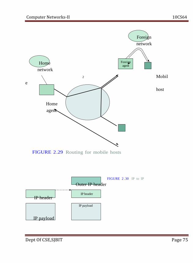
Computer Networks-II 10CS64
Foreign
network
Foreign agent
2
Routing for mobile hosts
FIGURE 2 .30 IP to IP
Outer IP header
IP header
IP payload
Home
network
e
Home
agent
FIGURE 2.29
IP header
IP payload
Dept Of CSE,SJBIT
Mobil
host
Page 75
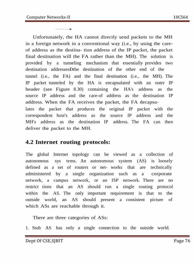
Computer Networks-II 10CS64
Unfortunately, the HA cannot directly send packets to the MH
in a foreign network in a conventional way (i.e., by using the care-
of address as the destina- tion address of the IP packet, the packet
final destination will the FA rather than the MH). The solution is
provided by a tunneling mechanism that essentially provides two
destination addressesÐthe destination of the other end of the
tunnel (i.e., the FA) and the final destination (i.e., the MH). The
IP packet tunneled by the HA is encapsulated with an outer IP
header (see Figure 8.30) containing the HA's address as the
source IP address and the care-of address as the destination IP
address. When the FA receives the packet, the FA decapsu-
lates the packet that produces the original IP packet with the
correspondent host's address as the source IP address and the
MH's address as the destination IP address. The FA can then
deliver the packet to the MH.
4.2 Internet routing protocols:
The global Internet topology can be viewed as a collection of
autonomous sys tems. An autonomous system (AS) is loosely
defined as a set of routers or net- works that are technically
administered by a single organization such as a corporate
network, a campus network, or an ISP network. There are no
restrict tions that an AS should run a single routing protocol
within the AS. The only important requirement is that to the
outside world, an AS should present a consistent picture of
which ASs are reachable through it.
There are three categories of ASs:
1. Stub AS has only a single connection to the outside world.
Dept Of CSE,SJBIT Page 76

Computer Networks-II 10CS64
Stub AS is also called single-homed AS.
2. Multihomed AS has multiple connections to the outside world
but refuses to carry transit traffic (traffic that originates and
terminates in the outside world). Multihomed AS carries only
local traffic (traffic that originates or terminates in that AS).
3. Transit AS has multiple connections to the outside world and
can carry transit and local traffic.
Home network
Home
agent
2a
Internet
1
2b
FIGURE 4.31 Route optimization for mobile IP
For the purpose of AS identification, an AS needs to be
assigned with a globally unique AS number (ASN) that is
represented by a 16-bit integer and thus is limited to about
Dept Of CSE,SJBIT Page 77
Foreign
network
Foreign
agent
3
4

Computer Networks-II 10CS64
65,000 numbers. We show later how ASNs are used in exterior
routing. Care must be taken not to exhaust the AS space.
Currently, there are about 3500 registered ASs in the Internet.
Fortunately, a stub AS, which is the most common type, does
not need an ASN, since the stub AS prefixes are placed at the
provider's routing table. On the other hand, a transit AS needs
an ASN. At present, an organization may request an ASN from
the American Registry for Internet Numbers (ARIN) in North
America. Routing protocols in the Internet are arranged in a
hierarchy that involves two types of protocols: Interior Gateway
Protocol (IGP) and Exterior Gateway Protocol (EGP). IGP is
used for routers to communicate within an AS and relies on IP
addresses to construct paths. EGP is used for routers to
communicate among different ASs and relies on AS numbers to
construct AS paths. In this section we cover two popular IGPs:
Routing Information Protocol and Open Shortest Path First.
4.3 Multicast routing:
The routing mechanisms discussed so far assume that a
given source transmits its packets to a single destination. For
some applications such as teleconferencing, a source may want
to send packets to multiple destinations simultaneously. This
requirement calls for another type of routing called multicast
routing as illustrated in Figure 8.52. In the figure, source S
wants to transmit to destinations with multicast group G1.
Although the source can send each copy of the packet separately
to each destination by using conventional unicast routing, a
more efficient method would be to minimize the number of
copies. For example, when router 1 receives a packet from the
source, router 1 copies the packet to routers 2 and 5
simultaneously. Upon receipt of these packets, router 2 forwards
Dept Of CSE,SJBIT Page 78

Computer Networks-II 10CS64
the packet to its local network, and router 5 copies the packet to
routers 7 and 8. The packet will eventually be received by each
intended destination.
With multicast routing, each packet is transmitted once per
link. If unicast routing is used instead, the link between the
source and router 1 will carry four copies for each packet
transmitted. In general, the bandwidth saving with multi- cast
routing becomes more substantial as the number of destinations
increases.
There are many ways to generate a multicast tree. One
approach that is used in multicast backbone (MBONE) is called
reverse-path multicasting. MBONE is basically an overlay packet
network on the Internet supporting routing of IP multicast
packets (with Class D address
FIGURE 4.52 Multicast Gree rooted at source
2
3
7
3
4
2
1
4
3
2
Dept Of CSE,SJBIT
t 1
2
3
1
5
4
1
5
42
3
2
6
5
3
1 4
1
3
4
G1
8
G2 G1
Page 79
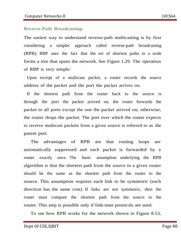
Computer Networks-II 10CS64 Reverse-Path Broadcasting:
The easiest way to understand reverse-path multicasting is by first
considering a simpler approach called reverse-path broadcasting
(RPB). RBP uses the fact that the set of shortest paths to a node
forms a tree that spans the network. See Figure 1.29. The operation
of RBP is very simple:
Upon receipt of a multicast packet, a router records the source
address of the packet and the port the packet arrives on.
If the shortest path from the router back to the source is
through the port the packet arrived on, the router forwards the
packet to all ports except the one the packet arrived on; otherwise,
the router drops the packet. The port over which the router expects
to receive multicast packets from a given source is referred to as the
parent port.
The advantages of RPB are that routing loops are
automatically suppressed and each packet is forwarded by a
router exactly once. The basic assumption underlying the RPB
algorithm is that the shortest path from the source to a given router
should be the same as the shortest path from the router to the
source. This assumption requires each link to be symmetric (each
direction has the same cost). If links are not symmetric, then the
router must compute the shortest path from the source to the
router. This step is possible only if link-state protocols are used.
To see how RPB works for the network shown in Figure 8.53,
Dept Of CSE,SJBIT Page 80
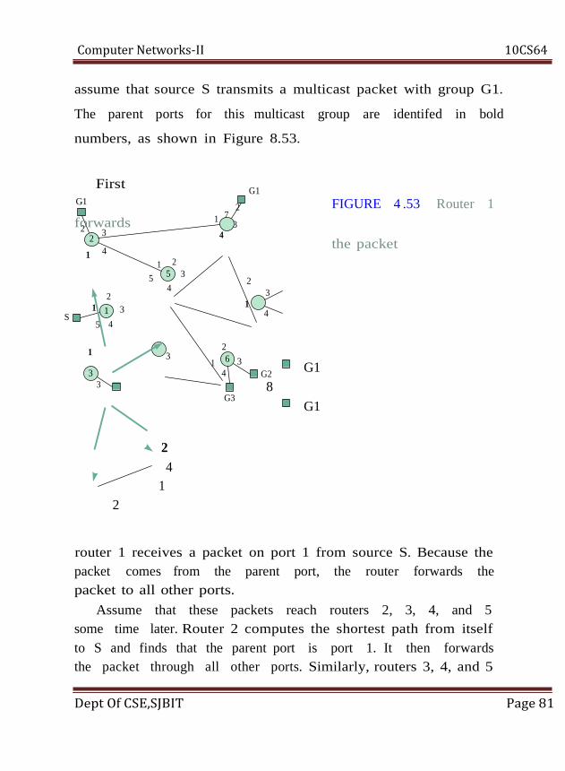
Computer Networks-II 10CS64
assume that source S transmits a multicast packet with group G1.
The parent ports for this multicast group are identifed in bold
numbers, as shown in Figure 8.53.
G1
FIGURE 4 .53 Router 1
2
the packet
2
3
1 4
4
3 G2
8
2
4
1
2
router 1 receives a packet on port 1 from source S. Because the
packet comes from the parent port, the router forwards the
packet to all other ports.
Assume that these packets reach routers 2, 3, 4, and 5
some time later. Router 2 computes the shortest path from itself
to S and finds that the parent port is port 1. It then forwards
the packet through all other ports. Similarly, routers 3, 4, and 5
Dept Of CSE,SJBIT Page 81
3
4
2
1
5
1
3
3
2
1
1 S
First
G1
forwards
2 7
3
3
1
1
5
3
1
4
2
5
4
3 2
6
4
G3
G1
G1
Computer Networks-II 10CS64
find that the packet arrives on the parent ports. As a result, each
router forwards the packet to its other ports, as shown in Figure
8.54. Note that the bidirectional link indicates that each router
forwards the packet to the other.
Next assume that the pG1ckets arrive at routers 2 through 8.
Because router 2 receives the packet from port 4, which is not
the parent port, router 2 drops the packet. Routers 3, 4, and 5
also drop the packet fo r the same reason. Router 6,however,
finds that the parent po rt is port 1, so router 6 forwards the
packet coming from router 4 to its other ports. The packet that
came from router 5 to router 6 is dropped. Routers 7 and 8
forward the packet that from router 5. Figure 8.55
illustrates the process pictorially. The reader should verify that
the packet will no longer be propagated after this point.
Note that although the hosts connected to routers 3 and 6
belong to different multicast groups, the packets for group G1 are
still forwarded by these routers. Typically, these hosts are
attached to the router via a shared medium LAN.
Therefore, unnecessary bandwidth is wasted regardless of the
multicast group.
This problem can be solved by having the router truncate its
transmission to the local network if none of the hosts attached to
the network belong to the multicast group. This refinement is
called truncated reverse-path broadcasting (TRPB).
Note that TRPB performs truncation only at the ``leaf'' routers
(routers at the edge of the network). The next section describes a
protocol that allows a router to determine which hosts belong to
which multicast groups.
Dept Of CSE,SJBIT Page 82
a
2
3
2
came
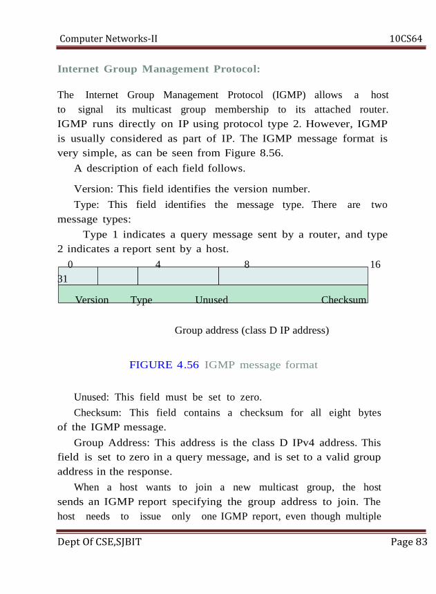
Computer Networks-II 10CS64
Internet Group Management Protocol:
The Internet Group Management Protocol (IGMP) allows a host
to signal its multicast group membership to its attached router.
IGMP runs directly on IP using protocol type 2. However, IGMP
is usually considered as part of IP. The IGMP message format is
very simple, as can be seen from Figure 8.56.
A description of each field follows.
Version: This field identifies the version number.
Type: This field identifies the message type. There are two
message types:
Type 1 indicates a query message sent by a router, and type
2 indicates a report sent by a host.
0 4 8 16
31
Version Type Unused Checksum
Group address (class D IP address)
FIGURE 4.56 IGMP message format
Unused: This field must be set to zero.
Checksum: This field contains a checksum for all eight bytes
of the IGMP message.
Group Address: This address is the class D IPv4 address. This
field is set to zero in a query message, and is set to a valid group
address in the response.
When a host wants to join a new multicast group, the host
sends an IGMP report specifying the group address to join. The
host needs to issue only one IGMP report, even though multiple
Dept Of CSE,SJBIT Page 83
Computer Networks-II 10CS64
applications are joining the same group. The host does not issue
a report if it wants to leave the group.
To make sure that multiple hosts do not send a report at the
same time when receiving a query that would lead to a collision,
the scheduled transmission time should be randomized. Because
the router only has to know that at least one host belongs to a
particular group, efficiency can be improved by having a host
monitor if another host sends the same report earlier than its
scheduled transmission. If another host has already sent the
same report, the first host cancels its report.
Reverse-Path Multicasting:
As section 8.8.2 just explained IGMP allows hosts to
indicate their group members. We now continue with selective
multicast routing called reverse-path multicasting (RPM), which
is an enhancement of TRPB. Unlike TRPB, RPM forwards a
multicast packet only to a router that will lead to a leaf router
with group members. Each router forwards the first packet for a
given (source, group) according to TRPB. All leaf routers receive
at least the first multicast packet. If a leaf router does not find a
member for this group on any of its ports, the leaf router will send
a prune message to its upstream router instructing the upstream
router not to forward subsequent packets belonging to this
(source, group). If the upstream router receives the prune
messages from all of its downstream neighbors, it will in turn
generate a prune message to its further upstream router.
A host may later decide to join a multicast group after a prune
message has been sent by its leaf router. In this case the leaf router
would send a graft message to its upstream router to cancel its
earlier prune message. Upon receiving the graft message, the first
Dept Of CSE,SJBIT Page 84
Computer Networks-II 10CS64
upstream router will forward subsequent multicast pack- ets to this
leaf router. If the first upstream router has also sent a prune
message earlier, the first upstream router will send a graft message
to the second upstream router. Eventually, a router in the multicast
tree will reactivate its affected port so that the multicast packets
will travel downstream toward the host. Figure 8.57 shows the
grafting message flow when a host attached to router 6 wants to
join the group. Subsequently, router 1 will forward the multicast
packets to router 4, which will forward the multicast packets to
router 6. Eventually, the multicast packets arrive at the host.
4.4 DHCP:
The Dynamic Host Configuration Protocol (DHCP) is a network
protocol that is used to configure network devices so that they can
communicate on an IP network. A DHCP client uses the DHCP protocol
to acquire configuration information, such as an IP address, a default
route and one or more DNS server addresses from a DHCP server. The
DHCP client then uses this information to configure its host. Once the
configuration process is complete, the host is able to communicate on
that internet. The DHCP server maintains a database of available IP
addresses and configuration information. When it receives a request from
a client, the DHCP server determines the network to which the DHCP
client is connected, and then allocates an IP address or prefix that is
appropriate for the client, and sends configuration information appropriate
for that client.
Because the DHCP protocol must work correctly even before DHCP
Dept Of CSE,SJBIT Page 85

Computer Networks-II 10CS64
clients have been configured, the DHCP server and DHCP client must be
connected to the same network link. In larger networks, this is not
practical. On such networks, each network link contains one or more
DHCP relay agents. These DHCP relay agents receive messages from
DHCP clients and forward them to DHCP servers. DHCP servers send
responses back to the relay agent, and the relay agent then sends these
responses to the DHCP client on the local network link.
DHCP servers typically grant IP addresses to clients only for a
limited interval. DHCP clients are responsible for renewing their IP
address before that interval has expired, and must stop using the address
once the interval has expired, if they have not been able to renew it.
DHCP is used for IPv4 and IPv6. While both versions serve much the
same purpose, the details of the protocol for IPv4 and IPv6 are sufficiently
different that they may be considered separate protocols.
Hosts that do not use DHCP for address configuration may still use it
to obtain other configuration information. Alternatively, IPv6 hosts may
use stateless address auto configuration. IPv4 hosts may use link-local
addressing to achieve limited local connectivity.
Dept Of CSE,SJBIT Page 86

Computer Networks-II 10CS64
4.5 NAT and Mobile IP:
The concept of NAT is a very powerful concept for several reasons:
It shields computers in a private LAN from the Internet and therefore reduces
the risks that are associated with connecting a computer to the Internet (hacking
attacks).More importantly, Internet service providers usually assignone IP address
to a home network or multiple IP addresses to an organization. However, the
number of computers on the home network. What NAT does is that local
Dept Of CSE,SJBIT Page 87
Computer Networks-II 10CS64
addresses (in one of the 3 ranges of private IP addresses that start with 10,172, or
192) are translated to one public IP address assigned to the home network (in the
case of DSL service) or multiple public IP addresses assigned to the organization
by the Internet service provider (in the case of organizations such as KFUPM ).
The NAT system also translates from the public IP address(es) to the
corresponding private IP addresses as the packets arrive from the Internet to the
private network. In fact, all computers in a network that uses NAT appear to the
outside world as having only few IP addresses.
For the case of a home network, all computers in your home network will
appear to the outside world as having a single IP address. If you visit a website
that records your IP address from one of your home network computers and then
try to visit the same website from another computer, the website will not be able to
distinguish between the two computers. The following are two examples that show
how NAT works. In the first case, the network is assigned multiple public IP
addresses equal to the number of machines in the network. All that the NAT does
is translate each private IP address into one of the public IP addresses and vice
versa. The two situations for outgoing packets (packets going from the private
network to the Internet) and incoming packets (packets going from the Internet to
the private network) are shown below. In the second case, the network is assigned
a single public IP address that will be used by all computers in the private
network. The two situations for outgoing packets and incoming packets are shown
afterwards.
Dept Of CSE,SJBIT Page 88

Computer Networks-II 10CS64
Mobile IP:
Mobile IP (or IP mobility) is an Internet Engineering Task Force (IETF)
standard communications protocol that is designed to allow mobile device users to
move from one network to another while maintaining a permanent IP address.
Mobile IP for IPv4 is described in IETF RFC 5944, and extensions are defined in
IETF RFC 4721. Mobile IPv6, the IP mobility implementation for the next
generation of the Internet Protocol, IPv6, is described in RFC 6275.
The Mobile IP protocol allows location-independent routing of IP datagrams
on the Internet. Each mobile node is identified by its home address disregarding its
current location in the Internet. While away from its home network, a mobile node
Dept Of CSE,SJBIT Page 89
Computer Networks-II 10CS64
is associated with a care-of address which identifies its current location and its
home address is associated with the local endpoint of a tunnel to its home agent.
Mobile IP specifies how a mobile node registers with its home agent and how the
home agent routes datagrams to the mobile node through the tunnel.
Applications:
In many applications (e.g., VPN, VoIP), sudden changes in network
connectivity and IP address can cause problems. Mobile IP was designed to
support seamless and continuous Internet connectivity.
Mobile IP is most often found in wired and wireless environments where
users need to carry their mobile devices across multiple LAN subnets. Examples
of use are in roaming between overlapping wireless systems, e.g., IP
over DVB, WLAN, WiMAX and BWA.
Changes in IPv6 for Mobile IPv6
•A set of mobility options to include in mobility messages
•A new Home Address option for the Destination Options header
•A new Type 2 Routing header
•New Internet Control Message Protocol for IPv6 (ICMPv6) messages to discover
the set of home agents and to obtain the prefix of the home link
•Changes to router discovery messages and options and additional Neighbor
Discovery options.
Dept Of CSE,SJBIT Page 90

Computer Networks-II 10CS64
PART – B
Dept Of CSE,SJBIT Page 91

Computer Networks-II 10CS64
UNIT - 5
Applications, Network Management, Network Security:
Application layer overview, Domain Name System (DNS), Remote
Login Protocols, E-mail, File Transfer and FTP, World Wide Web and
HTTP, Network management, Overview of network security,
Overview of security methods, Secret-key encryption protocols, Public-
key encryption protocols, Authentication, Authentication and digital
signature, Firewalls.
Dept Of CSE,SJBIT Page 92
Computer Networks-II 10CS64
UNIT-5
Applications, Network Management, Network Security
5.1. Application-Layer Overview
The application layer is built on the transport layer and provides network services to
user applications. The application layer defines and performs such applications as
electronic mail (e-mail), remote access to computers, file transfers, newsgroups, and
the Web, as well as streaming video, Internet radio and telephony, P2P file sharing,
multiuser networked games, streaming stored video clips, and real-time video
conferencing.
The application layer has its own software dependencies. When a new application is
developed, its software must be able to run on multiple machines, so that it does not
need to be rewritten for networking devices, such as routers, that function at the
network layer. In a client/server architecture for example, a client end host requests
services from a server host. A client host can be on sometimes or always. Figure 5.1
shows an example of application-layer communication.
Dept Of CSE,SJBIT Page 93

Computer Networks-II 10CS64
Figure 5.1. Web communication between two end systems
5.1.1. Client and Server Model
A client/server model provides specific computational services, such as partial-time
usage services to multiple machines. Reliable communication protocols, such as TCP,
allow interactive use of remote servers as well. For example, we can build a server that
provides remote image-processing services to clients. Implementing such a
communication service requires a server loaded with the application protocol to accept
requests and a client to make such requests. To invoke remote image processing, a user
first executes a client program establishing a TCP connection to a server. Then, the
client begins transmitting pieces of a raw image to the server. The server processes the
received objects and sends the results back.
5.2. Domain Name System (DNS)
Dept Of CSE,SJBIT Page 94
Computer Networks-II 10CS64
One of the most important components of the application layer is the Domain Name
System (DNS) server. DNS is a distributed hierarchical and global directory that
translates machine or domain names to numerical IP addresses.DNS can run over
either UDP or TCP. Some of the information-processing functions a DNS server
handles are
• Finding the address of a particular host
• Delegating a subtree of server names to another server
• Denoting the start of the subtree that contains cache and configuration parameters, and
giving corresponding addresses
• Naming a host that processes incoming mail for the designated target
• Finding the host type and the operating system information
• Finding an alias for the real name of a host
• Mapping IP addresses to host names
5.2.1. Domain Name Space
Any entity in the TCP/IP environment is identified by an IP address, which thereby
identifies the connection of the corresponding host to the Internet. An IP address can
also be assigned a domain name. Unique domain names assigned to hosts must be
selected from a name space and are generally organized in a hierarchical fashion.
Domain names are defined in a tree-based structure with the root at the top, as shown
in Figure 5.2. A tree is structured with a maximum of 128 levels, starting at level 0
(root). Each level consists of nodes. A node on a tree is identified by a label, with a
string of up to 63 characters, except for the root label, which has empty string.
Dept Of CSE,SJBIT Page 95
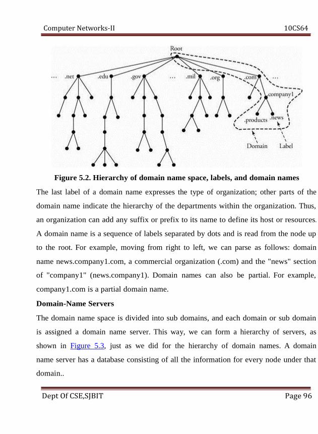
Computer Networks-II 10CS64
Figure 5.2. Hierarchy of domain name space, labels, and domain names
The last label of a domain name expresses the type of organization; other parts of the
domain name indicate the hierarchy of the departments within the organization. Thus,
an organization can add any suffix or prefix to its name to define its host or resources.
A domain name is a sequence of labels separated by dots and is read from the node up
to the root. For example, moving from right to left, we can parse as follows: domain
name news.company1.com, a commercial organization (.com) and the "news" section
of "company1" (news.company1). Domain names can also be partial. For example,
company1.com is a partial domain name.
Domain-Name Servers
The domain name space is divided into sub domains, and each domain or sub domain
is assigned a domain name server. This way, we can form a hierarchy of servers, as
shown in Figure 5.3, just as we did for the hierarchy of domain names. A domain
name server has a database consisting of all the information for every node under that
domain..
Dept Of CSE,SJBIT Page 96

Computer Networks-II 10CS64
Figure 5.3. Hierarchy of DNS domain name servers
5.2.2. Name/Address Mapping
DNS operates based on the client/server application. Any client host can send an IP
address to a domain name server to be mapped to a domain name. Each host that needs
to map an address to a name or vice versa should access the closest DNS server with
its request.
Mapping can be of either recursive or iterative. In recursive mapping (Figure 5.4), the
client host makes the request to its corresponding DNS server. The DNS server is
responsible for finding the answer recursively. The requesting client host asks for the
answer through its local DNS server, news.company1.com
Finally, .com server sends the query to the local DNS server of the requested place, as
Dept Of CSE,SJBIT Page 97
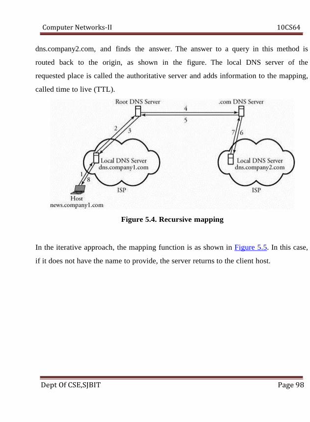
Computer Networks-II 10CS64
dns.company2.com, and finds the answer. The answer to a query in this method is
routed back to the origin, as shown in the figure. The local DNS server of the
requested place is called the authoritative server and adds information to the mapping,
called time to live (TTL).
Figure 5.4. Recursive mapping
In the iterative approach, the mapping function is as shown in Figure 5.5. In this case,
if it does not have the name to provide, the server returns to the client host.
Dept Of CSE,SJBIT Page 98

Computer Networks-II 10CS64
Figure 5.5. Iterative mapping
In Figure 5.5, the news.company1.com host sends the query to its own local DNS
server, dns.company1.comthus trying the root DNS server firstand then tries .com
server, finally ending up with the local DNS server of the requested place:
dns.company2.com.
5.2.3. DNS Message Format
DNS communication is made possible through query and reply messages. Both
message types have the 12-byte header format shown in Figure 5.6.
Dept Of CSE,SJBIT Page 99

Computer Networks-II 10CS64
Figure 5.6. DNS message format
The header has six fields as follows. A client uses the identification field to match the
reply with the query. This field may appear with a different number each time a client
transmits a query. The server copies this number in its reply. The flags field contains
subfields that represent the type of the message, such as the type of answer requested
or requested DNS recursive or iterative mapping. The number of questions field
indicates how many queries are in the question portion of the message. The number of
answers shows how many answers are in the answer field. For the query message, this
field contains all zeros. The number of authoritative records field consists of the
number of authoritative records in the authority portion of a reply message. Similarly,
this field is filled by zeros for a query message. Finally, the number of additional
records field records are in the additional information portion of a reply message and is
similarly filled by zeros in a query message.
5.3. Remote Login Protocols
A client/server model can create a mechanism that allows a user to establish a session
on the remote machine and then run its applications. This application is known as
remote login. This can be done by a client/server application program for the desired
service. Two remote login protocols are TELNET and SSH.
5.3.1. TELNET Protocol
TELNET (terminal network) is a TCP/IP standard for establishing a connection to a
remote system. TELNET allows a user to log in to a remote machine across the
Internet by first making a TCP connection and then pass the detail of the application
Dept Of CSE,SJBIT Page 100
Computer Networks-II 10CS64
from the user to the remote machine..
Logging to Remote Servers
With TELNET, an application program on the user's machine becomes the client. The
user's keyboard and its monitor also attach directly to the remote server. The remote-
logging operation is based on timesharing, whereby an authorized user has a login
name and a password. TELNET has the following properties.
• Client programs are built to use the standard client/server interfaces without knowing
the details of server programs.
• A client and a server can negotiate data format options.
• Once a connection is established through TELNET, both ends of the connection are
treated symmetrically.
When a user logs in to a remote server, the client's terminal driver accepts the
keystrokes and interprets them as characters by its operating system. Characters are
typically transformed to a universal character set called network virtual terminal
(NVT), which uses 7-bit USASCII representation for data. The client then establishes
a TCP connection to the server. Texts in the NVT format are transmitted using a TCP
session and are delivered to the operating system of the remote server. The server
converts the characters back from NVT to the local client machine's format.
5.3.2. Secure Shell (SSH) Protocol
Secure Shell (SSH), another remote login protocol, is based on UNIX programs. SSH
uses TCP for communications but is more powerful and flexible than TELNET and
allows the user to more easily execute a single command on a remote client. SSH has
the following advantages over TELNET.
• SSH provides a secure communication by encrypting and authenticating messages.
Dept Of CSE,SJBIT Page 101
Computer Networks-II 10CS64
• SSH provides several additional data transfers over the same connection by
multiplexing multiple channels that are used for remote login.
SSH security is implemented by using public-key encryption between the client and
remote servers. When a user establishes a connection to a remote server, the data being
transmitted remains confidential even if an intruder obtains a copy of the packets sent
over an SSH connection. SSH also implements an authentication process on messages
so that a server can find out and verify the host attempting to form a connection.
Normally, SSH requires users to enter a private password.
The advantage of port forwarding is that application data can be passed between two
sites the client and the second server without requiring a second client and server the
first server as a client and the second server.Figure 5.7 shows the format of an SSH
packet.
Figure 5.7. SSH packet format
• Length indicates the size of the packet, not including the length field or the variable-
length random padding field that follows it.
Dept Of CSE,SJBIT Page 102

Computer Networks-II 10CS64
• Padding causes an intrusion to be more difficult.
• Type identifies the type of message.
• CRC, or cyclic redundancy check, is an error-detection field.
Dept Of CSE,SJBIT Page 103

Computer Networks-II 10CS64
5.4. Electronic Mail (E-mail)
5.4.1. Simple Mail Transfer Protocol (SMTP) and E-mail
The Simple Mail Transfer Protocol (SMTP) plays a major role in transferring
Internet electronic mail. This protocol transfers electronic mail (e-mail ) from
the mail server of a source to the mail servers of destinations. SMTP is older
than the Hypertext Transfer Protocol (HTTP), the Web communication
protocol, and imposes certain restrictions, such as limits on the size of e-mail
content.
In Figure 5.8, user 1 is in a residential area, has an Internet service provider
(ISP), and is sending an e-mail to user 2, working in an organization. Suppose
that the mail servers are isp.com and organization.com, respectively. Thus,
user 1 and user 2 have e-mail addresses of [email protected] and
[email protected], respectively. The procedure for an e-mail exchange
between user 1 and user 2 is as follows.
Figure 5.8. Two users exchanging e-mail through SMTP
Dept Of CSE,SJBIT Page 104
Computer Networks-II 10CS64
Begin SMTP Between Two Users
1. User 1 provides user 2's e-mail address ([email protected]) and
composes its message.
2. User 1 sends the message to its mail server (isp.com).
3. Server isp.com places the message in its queue.
4. SMTP on user 1's mail server notices the message in the queue and opens a
TCP connection with the organization mail server (organization.com).
5. Initial SMTP handshaking takes place between the two servers.
6. The message is sent to organization.com's mail server, using the established
TCP connection.
7. User 2's mail server receives the message and then puts it in user 2's mailbox,
ready to be retrieved by user 2.
5.5. File Transfer and FTP
File transfer is another computer networking application. It is always
essential that files and information geographically distributed over
different locations be shared among the members of a working group.
In a certain application, files are typically saved in a server. A user
then uses a file transfer protocol to access the server and transfer the
desired file. Two file transfer protocols are FTP and SCP.
5.5.1. File Transfer Protocol (FTP)
File Transfer Protocol (FTP) is part of the TCP/IP suite and is very
Dept Of CSE,SJBIT Page 105

Computer Networks-II 10CS64
similar to TELNET. Both FTP and TELNET are built on the
client/server paradigm, and both allow a user to establish a remote
connection. However, TELNET provides a broader access to a user,
whereas FTP allows access only to certain files. The essence of this
protocol is as follows.
Begin File Transfer Protocol
1. A user requests a connection to a remote server.
2. The user waits for an acknowledgment.
3. Once connected, the user must enter a user ID, followed by a
password.
4. The connection is established over a TCP session.
5. The desired file is transferred.
6. The user closes the FTP connection.
FTP can also run through a Web browser.
5.5.2. Secure Copy Protocol (SCP)
The Secure Copy Protocol (SCP) is similar to TELNET but is secure.
Incorporated in the SCP structure are a number of encryption and
authentication features that are similar to those in SSH. Also similar
is the exchange of commands between local and remote hosts. SCP
commands automatically prompt the user for the password
information when it is time to access a remote machine. SCP cannot
handle file transfer between machines of significantly different
architectures.
Dept Of CSE,SJBIT Page 106
Computer Networks-II 10CS64
5.6. World Wide Web (WWW) and HTTP
Application-layer software is the intelligence built for end servers. The World
Wide Web (WWW), or simply Web, is a global network of servers linked by
a common protocol allowing access to all connected hypertext resources.
When a client host requests an object, a Web server responds by sending the
requested object through browsing tools. A browser is a user agent displaying
the requested Web page. The Hyper Text Transfer Protocol (HTTP) transfers
that page at the application layer. HTTP uses TCP rather than UDP, since
reliability of delivery is important for Web pages with text. The TCP
connection-establishment delay in HTTP is one of the main contributing
delay factors associated with downloading Web documents.
HTTP is based on the client/server idea, having a client and a server program,
both of which can be executed on different end systems. The communication
is carried out through an exchange of HTTP messages. This protocol
specifies the structure of these messages. For example, HTTP defines how a
pair of client/server hosts should exchange messages. In this context, a Web
page consists of files, such as Hypertext Mark-up Language (HTML) file or
an image that can be addressed by a single uniform resource locator (URL).
A URL is a global address of an HTML document and has two parts. The
first part indicates what protocol is used, and the second part determines the
IP address of the associated resource.
5.6.1. Web Caching (Proxy Server)
An HTTP request from a user is first directed to the network proxy server, or
Web cache. Once configured by the network, a browser's request for an
Dept Of CSE,SJBIT Page 107

Computer Networks-II 10CS64
object is directed to the Web cache, which must contain updated copies of all
objects in its defined proximity. The main reason for Web caching is to
reduce the response time for a user request. This benefit is much more
obvious when the bandwidth to a requested server is limited because of traffic
at certain hours of the day. Normally, each organization or ISP should have
its own cache providing a high-speed link to its users. Consequently, it is to
users' advantages that this rapid method of finding objects be available. This
method of Internet access also reduces traffic on an organization's access link
to the Internet. The details of Web caching are as follows:
Begin Web Caching Algorithm
1. The source browser makes a TCP connection to the Web cache.
2. The user browser transmits its HTTP request to the Web cache.
3. If it has a copy of the requested object, the Web cache forwards the object to
the user browser.
Otherwise the Web cache establishes a TCP connection to the requested
server and asks for the object. Once it receives the requested object, the Web
cache stores a copy of it and forwards another copy to the requesting user
browser over the existing TCP connection.
Figure 5.9 shows three Internet service providers (ISPs). A user in ISP
domain 3 is browsing to find and watch an object named
http://www.filmmaker.com in ISP domain 1. The request for this object is
directed to the Web cache, shown by dashed lines. In this example, the Web
cache has no record of the requested object and therefore is establishing
another TCP connection to update its record.
Dept Of CSE,SJBIT Page 108

Computer Networks-II 10CS64
Figure 5.9. A user's browser requesting an object through the
Web cache
5.7. Network Management
The main purpose of network management is to monitor, manage, and control
a network. A network can be structured with many links, routers, servers, and
other physical-layer devices, which can be equipped with many network
protocols that coordinate them. Imagine when thousands of such devices or
protocols are tied together by an ISP and how drastic their management can
become to avoid any interruptions in routine services. In this context the
purpose of network management is to monitor, test, and analyze the
hardware, software, and human elements of a network and then to configure
and control those elements to meet the operational performance requirements
Dept Of CSE,SJBIT Page 109

Computer Networks-II 10CS64
of the network.
Figure 5.10 illustrates a simple network management scenario in which LANs
connect to the Internet. LAN 1 is dedicated to the network administrator
facilities. The network administrator can periodically send management
packets to communicate with a certain network entity. A malfunctioning
component in a network can also initiate communication of its problem to the
network administrator.
Figure 5.10. Simple network management in a scenario of LANs
connecting to the Internet
Network management tasks can be characterized as follows:
• QoS and performance management. A network administrator periodically
Dept Of CSE,SJBIT Page 110

Computer Networks-II 10CS64
monitors and analyzes routers, hosts, and utilization of links and then redirect
traffic flow to avoid any overloaded spots. Certain tools are available to
detect rapid changes in traffic flow.
• Network failure management. Any fault in a network, such as link, host, or
router hardware or software outages, must be detected, located, and
responded to by the network. Typically, increased checksum errors in frames
is an indication of possible error. Figure 5.10 shows adapter failures at router
R3 and host H37; these failures can be detected through network
management.
• Configuration management. This task involves tracking all the devices under
management and ensuring that all devices are connected and operate
properly. If there is an unexpected change in routing tables, a network
administrator wants to discover the misconfigured spot and reconfigure the
network before the error affects the network substantially.
• Security management. A network administrator is responsible for the security
of its network. This task is handled mainly through firewalls. A firewall can
monitor and control access points. In such cases, the network administrator
wants to know about any intrusion from a suspicious source to the network.
For example, a host in a network can be attacked by receiving a large number
of SYN packets.
• Billing and accounting management. The network administrator specifies
user access or restrictions to network resources and issues all billing and
charges, if any, to users.
Locating a failing point, such as an adapter failure at a host or a router, can be
Dept Of CSE,SJBIT Page 111
Computer Networks-II 10CS64
done by appropriate network management tools. Normally, a standard packet
format is specified for network management.
5.7.1. Elements of Network Management
Network management has three main components: network management: a
managing center, a managed device, and a network management protocol.
The managing center consists of the network administrator and his or her
facilities. Typically, the managing center comprises a substantial human
network. A managed device is the network equipment, including its software,
that is controlled by the managing center. Any hub, bridge, router, server,
printer, or modem can be a managed device. The network management
protocol is a policy between the managing center and the managed devices.
The protocol in this context allows the managing center to obtain the status of
managed devices. In network management, an agent is a managed device,
such as a router, hub, or bridge. A manager is a network administrative
device, as a management host. An agent can use the network management
protocol to inform the managing center of an unexpected event.
5.7.2. Structure of Management Information (SMI)
The structure of management information (SMI) language is used to define
the rules for naming objects and to encode objects in a managed network
center. In other words, SMI is a language by which a specific instance of the
data in a managed network center is defined. For example, Integer32 means a
32-bit integer with a value between -231 and -231 - 1. The SMI language also
provides higher-level language constructs, which typically specify the data
type, status, and semantics of managed objects containing the management
Dept Of CSE,SJBIT Page 112
Computer Networks-II 10CS64
data. For example, the STATUS clause specifies whether the object definition
is current or obsolete, ipInDelivers defines a 32-bit counter to trace the
number of IP datagrams received at a managed device and then received at an
upper-layer protocol.
5.7.3. Management Information Base (MIB)
Management information base (MIB) is an information storage medium that
contains managed objects reflecting the current status of the network.
Because managed objects have associated pieces of information that are
stored in a MIB, the MIB forms a collection of named objects, including their
relationships to one another in a management center. The information pieces
can be obtained by directing the managing center to do so.
Objects are organized in a hierarchical manner and are identified by the
abstract syntax notation one (ASN.1) object definition language. The
hierarchy of object names, known as ASN.1 object identifier, is an object
identifier tree in which each branch has both a name and a number, as shown
in Figure 5.11. Network management can then identify an object by a
sequence of names or numbers from the root to that object.
Dept Of CSE,SJBIT Page 113
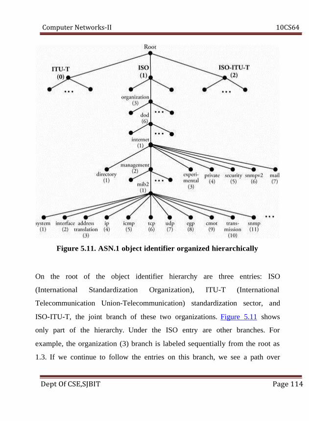
Computer Networks-II 10CS64
Figure 5.11. ASN.1 object identifier organized hierarchically
On the root of the object identifier hierarchy are three entries: ISO
(International Standardization Organization), ITU-T (International
Telecommunication Union-Telecommunication) standardization sector, and
ISO-ITU-T, the joint branch of these two organizations. Figure 5.11 shows
only part of the hierarchy. Under the ISO entry are other branches. For
example, the organization (3) branch is labeled sequentially from the root as
1.3. If we continue to follow the entries on this branch, we see a path over
Dept Of CSE,SJBIT Page 114

Computer Networks-II 10CS64
dod (6), Internet (1), management (2), mib-2(1), and ip (4). This path is
identified by (1.3.6.1.2.1.4) to indicate all the labeled numbers from the root
to the ip (4) entry. Besides that entry, MIB module represents a number of
network interfaces and well-known Internet protocols at the bottom of this
tree. This path clearly shows all the standards of "IP" associated with the
"MIB-2" computer networking "management."
5.7.4. Simple Network Management Protocol (SNMP)
The Simple Network Management Protocol (SNMP) is designed to monitor
the performance of network protocols and devices. SNMP protocol data units
(PDUs) can be carried in the payload of a UDP datagram, and so its delivery
to a destination is not guaranteed. Managed devices, such as routers and
hosts, are objects, and each object has a formal ASN.1 definition. For each
object, MIB accommodates a database of information that describes its
characteristics. With this protocol, a network manager can find the location of
a fault. SNMP runs on top of UDP and uses client/server configurations. The
commands of this protocol define how to query information from a server and
forward information to a server or a client.
The task of SNMP is to transport MIB information among managing centers
and agents executing on behalf of managing centers. For each managed MIB
object, an SNMP request is used to retrieve or change its associated value. If
an unsolicited message is received by an agent, or when an interface or
device goes down, the protocol can also inform the managing center. The
second version of this protocol, SNMPv2, runs on top of more protocols and
has more messaging options, resulting in more effective network
Dept Of CSE,SJBIT Page 115
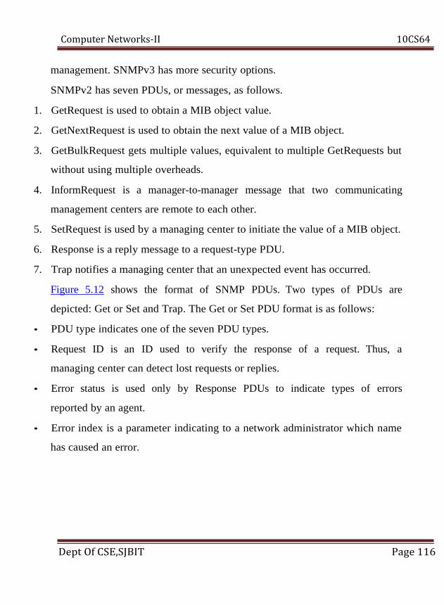
Computer Networks-II 10CS64
management. SNMPv3 has more security options.
SNMPv2 has seven PDUs, or messages, as follows.
1. GetRequest is used to obtain a MIB object value.
2. GetNextRequest is used to obtain the next value of a MIB object.
3. GetBulkRequest gets multiple values, equivalent to multiple GetRequests but
without using multiple overheads.
4. InformRequest is a manager-to-manager message that two communicating
management centers are remote to each other.
5. SetRequest is used by a managing center to initiate the value of a MIB object.
6. Response is a reply message to a request-type PDU.
7. Trap notifies a managing center that an unexpected event has occurred.
Figure 5.12 shows the format of SNMP PDUs. Two types of PDUs are
depicted: Get or Set and Trap. The Get or Set PDU format is as follows:
• PDU type indicates one of the seven PDU types.
• Request ID is an ID used to verify the response of a request. Thus, a
managing center can detect lost requests or replies.
• Error status is used only by Response PDUs to indicate types of errors
reported by an agent.
• Error index is a parameter indicating to a network administrator which name
has caused an error.
Dept Of CSE,SJBIT Page 116
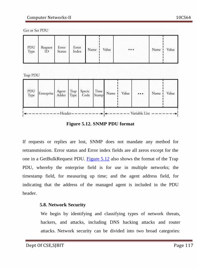
Computer Networks-II 10CS64
Figure 5.12. SNMP PDU format
If requests or replies are lost, SNMP does not mandate any method for
retransmission. Error status and Error index fields are all zeros except for the
one in a GetBulkRequest PDU. Figure 5.12 also shows the format of the Trap
PDU, whereby the enterprise field is for use in multiple networks; the
timestamp field, for measuring up time; and the agent address field, for
indicating that the address of the managed agent is included in the PDU
header.
5.8. Network Security
We begin by identifying and classifying types of network threats,
hackers, and attacks, including DNS hacking attacks and router
attacks. Network security can be divided into two broad categories:
Dept Of CSE,SJBIT Page 117

Computer Networks-II 10CS64
cryptographic techniques and authentication techniques
(verification). Both secret-key and public-key encryption protocols
are presented. We then discuss message authentication and digital
signature methods, through which a receiver can be assured that an
incoming message is from whom it says it is.
We then consider several standardized security techniques, such as
IPsec, and the security of wireless networks and IEEE 802.11
standards, as well as firewalls, or devices designed to protect a
network. Finally, we present a case study on the security of wireless
networks.
Dept Of CSE,SJBIT Page 118

Computer Networks-II 10CS64
5.8.1. Overview of Network Security
Network security is a top-priority issue in data networks. As communication
networks are growing rapidly, security issues have pushed to the forefront of
concern for end users, administrators, and equipment suppliers. Despite
enormous joint efforts by various groups to develop effective security
solutions for networks, hackers continue to pose new, serious threats by
taking advantage of weaknesses present in the Internet infrastructure.
Elements of Network Security
Network security is concerned mainly with the following two elements:
1. Confidentiality. Information should be available only to those who have
rightful access to it.
2. Authenticity and integrity. The sender of a message and the message itself
should be verified at the receiving point.
In Figure 5.13, user 1 sends a message ("I am user 1") to user 2. In part (a) of
the figure, the network lacks any security system, so an intruder can receive
the message, change its content to a different message ("Hi! I am user 1") and
send it to user 2. User 2 may not know that this falsified message is really
from user 1 (authentication) and that the content of the message is what user
1 (confidentiality). In part (b) of the figure, a security block is added to each
side of the communication, and a secret key that only users 1 and 2 would
know about is included. Therefore, the message is changed to a form that
cannot be altered by the intruder, who would be disabled in this
communication transaction.
Dept Of CSE,SJBIT Page 119
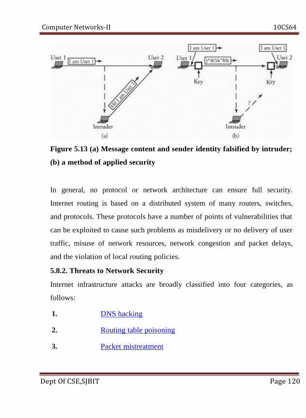
Computer Networks-II 10CS64
Figure 5.13 (a) Message content and sender identity falsified by intruder;
(b) a method of applied security
In general, no protocol or network architecture can ensure full security.
Internet routing is based on a distributed system of many routers, switches,
and protocols. These protocols have a number of points of vulnerabilities that
can be exploited to cause such problems as misdelivery or no delivery of user
traffic, misuse of network resources, network congestion and packet delays,
and the violation of local routing policies.
5.8.2. Threats to Network Security
Internet infrastructure attacks are broadly classified into four categories, as
follows:
1. DNS hacking
2. Routing table poisoning
3. Packet mistreatment
Dept Of CSE,SJBIT Page 120

Computer Networks-II 10CS64
4. Denial of service
Among these threats, the first three attacks are related to network
infrastructure; denial-of-service attacks are related to end systems.
DNS Hacking Attacks
The Domain Name System (DNS) server is a distributed hierarchical and
global directory that translates domain names into numerical IP address. DNS
is a critical infrastructure, and all hosts contact DNS to access servers and
start connections. In the normal mode of operation, hosts send UDP queries
to the DNS server. Servers reply with a proper answer, or direct the queries to
smarter servers. A DNS server also stores information other than host
addresses.
Name-resolution services in the modern Internet environment are essential for
e-mail transmission, navigation to Web sites, or data transfer. Thus, an attack
on DNS can potentially affect a large portion of the Internet. A DNS hacking
attack may result in the lack of data authenticity and integrity and can appear
in any of the following forms:
1. An information-level attack forces a server to correspond with other than the
correct answer. With cache poisoning, a hacker tricks a remote name server
into caching the answer for a third-party domain by providing malicious
information for the domain's authorized servers. Hackers can then redirect
traffic to a preselected site.
2. In a masquerading attack, the adversary poses as a trusted entity and obtains
all the secret information. In this guise, the attacker can stop any message
from being transmitted further or can change the content or redirect the
Dept Of CSE,SJBIT Page 121
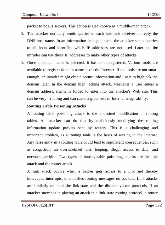
Computer Networks-II 10CS64
packet to bogus servers. This action is also known as a middle-man attack.
3. The attacker normally sends queries to each host and receives in reply the
DNS host name. In an information leakage attack, the attacker sends queries
to all hosts and identifies which IP addresses are not used. Later on, the
intruder can use those IP addresses to make other types of attacks.
4. Once a domain name is selected, it has to be registered. Various tools are
available to register domain names over the Internet. If the tools are not smart
enough, an invader might obtain secure information and use it to highjack the
domain later. In the domain high jacking attack, whenever a user enters a
domain address, she/he is forced to enter into the attacker's Web site. This
can be very irritating and can cause a great loss of Internet usage ability.
Routing Table Poisoning Attacks
A routing table poisoning attack is the undesired modification of routing
tables. An attacker can do this by maliciously modifying the routing
information update packets sent by routers. This is a challenging and
important problem, as a routing table is the basis of routing in the Internet.
Any false entry in a routing table could lead to significant consequences, such
as congestion, an overwhelmed host, looping, illegal access to data, and
network partition. Two types of routing table poisoning attacks are the link
attack and the router attack.
A link attack occurs when a hacker gets access to a link and thereby
intercepts, interrupts, or modifies routing messages on packets. Link attacks
act similarly on both the link-state and the distance-vector protocols. If an
attacker succeeds in placing an attack in a link-state routing protocol, a router
Dept Of CSE,SJBIT Page 122
Computer Networks-II 10CS64
may send incorrect updates about its neighbors or remain silent even if the
link state of its neighbor has changed. The attack through a link can be so
severe that the attacker can program a router to either drop packets from a
victim or readdress packets to a victim, resulting in a lower throughput of the
network. Sometimes, a router can stop an intended packet from being
forwarded further. However, since more than one path to any destination
exists, the packet ultimately reaches its destination.
Router attacks may affect the link-state protocol or even the distance-vector
protocol. If link-state protocol routers are attacked, they become malicious.
They may add a nonexisting link to a routing table, delete an existing link, or
even change the cost of a link. This attack may cause a router to simply
ignore the updates sent by its neighbors, leading to a serious impact on the
operability of the network traffic flow.
In the distance-vector protocol, an attacker may cause routers to send wrong
updates about any node in the network, thereby misleading a router and
resulting in network problems.
Most unprotected routers have no way to validate updates. Therefore, both
link-state and distance-vector router attacks are very effective. In the
distance-vector protocol, for example, a malicious router can send wrong
information in the form of a distance vector to all its neighbors. A neighbor
may not be able to detect this kind of attack and thus proceeds to update its
routing table, based on wrong distance vectors. The error can in turn be
propagated to a great portion of the network before being detected.
Packet-Mistreatment Attacks
Dept Of CSE,SJBIT Page 123

Computer Networks-II 10CS64
A packet-mistreatment attack can occur during any data transmission. A
hacker may capture certain data packets and mistreat them. This type of
attack is very difficult to detect. The attack may result in congestion,
lowering throughput, and denial-of-service attacks. Similar to routing table
poisoning attacks, packet-mistreatment attacks can also be subclassified into
link attacks and router attacks. The link attack causes interruption,
modification, or replication of data packets. A router attack can misroute all
packets and may result in congestion or denial of service. Following are some
examples of a packet-mistreatment attack:
• Interruption. If an attacker intercepts packets, they may not be allowed to be
propagated to their destinations, resulting in a lower throughput of the
network. This kind of attack cannot be detected easily, as even in normal
operations, routers can drop some packets, for various reasons.
• Modification. Attackers may succeed in accessing the content of a packet
while in transit and change its content. They can then change the address of
the packet or even change its data. To solve this kind of problem, a digital
signature mechanism, discussed later in this chapter, can be used.
• Replication. An attacker might trap a packet and replay it. This kind of attack
can be detected by using the sequence number for each packet.
• Ping of death. An attacker may send a ping message, which is large and
therefore must be fragmented for transport. The receiver then starts to
reassemble the fragments as the ping fragments arrive. The total packet
length becomes too large and might cause a system crash.
• Malicious misrouting of packets. A hacker may attack a router and change its
Dept Of CSE,SJBIT Page 124

Computer Networks-II 10CS64
routing table, resulting in misrouting of data packets, causing a denial of
service.
Denial-of-Service Attacks
A denial-of-service attack is a type of security breach that prohibits a user
from accessing normally provided services. The denial of service does not
result in information theft or any kind of information loss but can nonetheless
be very dangerous, as it can cost the target person a large amount of time and
money. Denial-of-service attacks affect the destination rather than a data
packet or router.
Usually, a denial-of-service attack affects a specific network service, such as
e-mail or DNS. For example, such an attack may overwhelm the DNS server
in various ways and make it inoperable. One way of initiating this attack is by
causing buffer overflow. Inserting an executable code inside memory can
potentially cause a buffer overflow. Or, an adversary may use various tools to
send large numbers of queries to a DNS server, which then is not able to
provide services in a timely manner.
Denial-of-service attacks are easy to generate but difficult to detect. They
take important servers out of action for few hours, thereby denying service to
all users. There are yet a few other situations that can cause this kind of
attack, such as UDP flood, a TCP flood and ICMP flood. In all these attacks,
the hacker's main aim is to overwhelm victims and disrupt services provided
to them.
Denial-of-service attacks are two types:
1. Single-source. An attacker sends a large number of packets to a target system
Dept Of CSE,SJBIT Page 125

Computer Networks-II 10CS64
to overwhelm and disable it. These packets are designed such that their real
sources cannot be identified.
2. Distributed. In this type of attack, a large number of hosts are used to flood
unwanted traffic to a single target. The target cannot then be accessible to
other users in the network, as it is processing the flood of traffic.
The flood may be either a UDP flood or a TCP SYN flood. UDP flooding is
used against two target systems and can stop the services offered by either
system. Hackers link the UDP character-generating services of a system to
another one by sending UDP packets with spoofed return addresses. This may
create an infinite looping between the two systems, leading to system
uselessness.
Normally, a SYN packet is sent by a host to a user who intends to establish a
connection. The user then sends back an acknowledgment. In the TCP SYN
flood, a hacker sends a large number of SYN packets to a target user. Since
the return addresses are spoofed, the target user queues up a SYN/ACK
packet and never processes it. Therefore, the target system keeps on waiting.
The result may be a hard disk crash or reboot.
5.8.2. Overview of Security Methods
Common solutions that can protect computer communication networks from
attacks are classified as cryptographic techniques or authentication techniques
(verification).
Dept Of CSE,SJBIT Page 126

Computer Networks-II 10CS64
Cryptographic Techniques
Cryptography has a long and fascinating history. Centuries ago, cryptography
was used as a tool to protect national secrets and strategies. Today, network
engineers focus on cryptography methods for computer communication
networks. Cryptography is the process of tranforming a piece of information
or message shared by two parties into some sort of code. The message is
scrambled before transmission so that it is undetectable by outside watchers.
This kind of message needs to be decoded at the receiving end before any
further processing.
The main tool that network security experts are using to encrypt a message M
is a secret key K; the fundamental operation often used to encrypt a message
is the Exclusive-OR ( ). Suppose that we have one bit, M, and a secret bit,
K. A simple encryption is carried out using M K. To decrypt this message,
the second partyif he/she has the key, Kcan easily detect M by performing the
following:
Equation 10.1
In computer communication networks, data can travel between two users
while it is encrypted. In Figure 5.14, two servers are exchanging data while
two types of encryption devices are installed in their communication network.
The first encryption device is end-to-end encryption, whereby secret coding is
carried out at both end systems.
Dept Of CSE,SJBIT Page 127
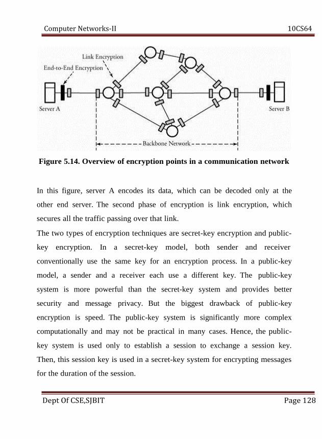
Computer Networks-II 10CS64
Figure 5.14. Overview of encryption points in a communication network
In this figure, server A encodes its data, which can be decoded only at the
other end server. The second phase of encryption is link encryption, which
secures all the traffic passing over that link.
The two types of encryption techniques are secret-key encryption and public-
key encryption. In a secret-key model, both sender and receiver
conventionally use the same key for an encryption process. In a public-key
model, a sender and a receiver each use a different key. The public-key
system is more powerful than the secret-key system and provides better
security and message privacy. But the biggest drawback of public-key
encryption is speed. The public-key system is significantly more complex
computationally and may not be practical in many cases. Hence, the public-
key system is used only to establish a session to exchange a session key.
Then, this session key is used in a secret-key system for encrypting messages
for the duration of the session.
Dept Of CSE,SJBIT Page 128

Computer Networks-II 10CS64
Authentication Techniques
Encryption methods offer the assurance of message confidentiality. However,
a networking system must be able to verify the authenticity of the message
and the sender of the message. These forms of security techniques in
computer networks are known as authentication techniques and are
categorized as authentication with message digest and authentication with
digital signature. Message authentication protects a user in a network against
data falsification and ensures data integrity. These methods do not necessarily
use keys.
5.9. Secret-Key Encryption Protocols
Secret-key encryption protocols, sometimes known as symmetric encryption,
or single-key encryption protocols, are conventional encryption models. They
typically consist of an encryption algorithm, a key, and a decryption
algorithm. At the end point, the encrypted message is called ciphertext.
Several standard mechanisms can be used to implement a secret-key
encryption algorithm. Here, we focus on two protocols: Data Encryption
Standard (DES) and Advanced Encryption Standard (AES).
In these algorithms, a shared secret key between a transmitter and a receiver
is assigned at the transmitter and receiver points. The encryption algorithm
produces a different key at any time for a specific transmission. Changing the
key changes the output of the algorithm. At the receiving end, the encrypted
information can be transformed back to the original data by using a
Dept Of CSE,SJBIT Page 129

Computer Networks-II 10CS64
decryption algorithm and the same key that was used for encryption. The
security of conventional encryption depends on the secrecy of the key, not on
the secrecy of the encryption algorithm. Consequently, the algorithm need not
be kept secret; only the key has to be secret.
5.9.1. Data Encryption Standard (DES)
With the Data Encryption Standard (DES), plaintext messages are converted
into 64-bit blocks, each encrypted using a key. The key length is 64 bits but
contains only 56 usable bits; thus, the last bit of each 8 byte in the key is a
parity bit for the corresponding byte. DES consists of 16 identical rounds of
an operation, as shown in Figure 5.15. The details of the algorithm on each
64-bit block of message at each round i of operation are as follows.
Begin DES Algorithm
1. Initialize. Before round 1 begins, all 64 bits of an incoming message and all
56 bits of the secret key are separately permuted (shuffled).
2. Each incoming 64-bit message is broken into two 32-bit halves denoted by Li
and Ri, respectively.
3. The 56 bits of the key are also broken into two 28-bit halves, and each half is
rotated one or two bit positions, depending on the round.
4. All 56 bits of the key are permuted, producing version ki of the key on round
i.
5. In this step, is a logic Exclusive-OR, and the description of function F()
appears next. Then, Li and Ri are determined by
Equation 10.2
Dept Of CSE,SJBIT Page 130

Computer Networks-II 10CS64
and
Equation 10.3
6. All 64 bits of a message are permuted.
Figure 5.3. The Data Encryption Standard (DES)
The operation of function F() at any round i of DES is as follows.
1. Out of 52 bits of ki, function F() chooses 48 bits.
2. The 32-bit Ri-1 is expanded from 32 bits to 48 bits so that it can be combined
with 48-bit ki. The expansion of Ri-1 is carried out by first breaking Ri-1 into
eight 4-bit chunks and then expanding each chunk by copying the leftmost bit
and the rightmost bit from left and right adjacent chunks, respectively.
Dept Of CSE,SJBIT Page 131

Computer Networks-II 10CS64
3. Function F() also partitions the 48 bits of ki into eight 6-bit chunks.
4. The corresponding eight chunks of Ri-1 and eight chunks of ki are combined
as follows:
Equation 10.4
At the receiver, the same steps and the same key are used to reverse the
encryption. It is now apparent that the 56-bit key length may not be sufficient
to provide full security. This argument is still controversial. Triple DES
provides a solution for this controversy: three keys are used, for a total of 168
bits. It should also be mentioned that DES can be implemented more
efficiently in hardware than in software.
5.9.2. Advanced Encryption Standard (AES)
The Advanced Encryption Standard (AES) protocol has a better security
strength than DES. AES supports 128-bit symmetric block messages and uses
128-, 192-, or 256-bit keys. The number of rounds in AES is variable from 10
to 14 rounds, depending on the key and block sizes. Figure 5.16 illustrates the
encryption overview of this protocol, using a 128-bit key. There are ten
rounds of encryptions for the key size of 128 bits. All rounds are identical
except for the last round, which has no mix-column stage.
Dept Of CSE,SJBIT Page 132
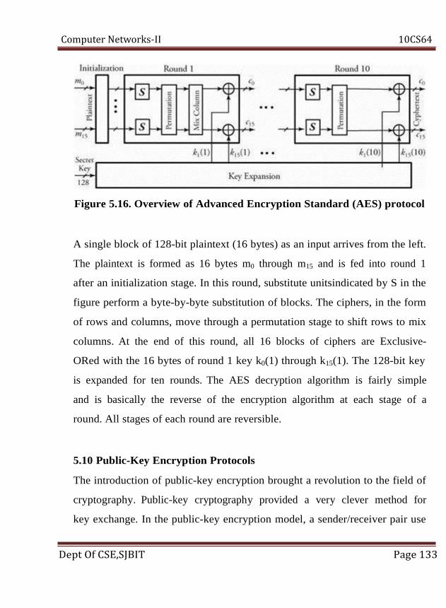
Computer Networks-II 10CS64
Figure 5.16. Overview of Advanced Encryption Standard (AES) protocol
A single block of 128-bit plaintext (16 bytes) as an input arrives from the left.
The plaintext is formed as 16 bytes m0 through m15 and is fed into round 1
after an initialization stage. In this round, substitute unitsindicated by S in the
figure perform a byte-by-byte substitution of blocks. The ciphers, in the form
of rows and columns, move through a permutation stage to shift rows to mix
columns. At the end of this round, all 16 blocks of ciphers are Exclusive-
ORed with the 16 bytes of round 1 key k0(1) through k15(1). The 128-bit key
is expanded for ten rounds. The AES decryption algorithm is fairly simple
and is basically the reverse of the encryption algorithm at each stage of a
round. All stages of each round are reversible.
5.10 Public-Key Encryption Protocols
The introduction of public-key encryption brought a revolution to the field of
cryptography. Public-key cryptography provided a very clever method for
key exchange. In the public-key encryption model, a sender/receiver pair use
Dept Of CSE,SJBIT Page 133

Computer Networks-II 10CS64
different keys. This model is sometimes known as asymmetric, or two-key,
encryption.
Public-key algorithm is based on mathematical functions rather than on
substitution or permutation, although the security of any encryption scheme
indeed depends on the length of the key and the computational work involved
in breaking an encrypted message. Several public-key encryption protocols
can be implemented. Among them, the following two protocols are the focus
of our study:
• Rivert, Shamir, and Aldeman (RSA) protocol
• Diffie-Hillman key-exchange protocol.
In the public-key encryption methods, either of the two related keys can be
used for encryption; the other one, for decryption. It is computationally
infeasible to determine the decryption key given only the algorithm and the
encryption key. Each system using this encryption method generates a pair of
keys to be used for encryption and decryption of a message that it will
receive. Each system publishes its encryption key by placing it in a public
register or file and sorts out the key as a public one.
The companion key is kept private. If A wishes to send a message to B, A
encrypts the message by using B's public key. On receiving the message, B
decrypts it with the private B key. No other recipients can decrypt the
message, since only B knows its private key. This way, public-key encryption
secures an incoming communication as long as a system controls its private
key. However, public-key encryption has extra computational overhead and is
more complex than the conventional one.
Dept Of CSE,SJBIT Page 134

Computer Networks-II 10CS64
5.10.1. RSA Algorithm
Rivert, Shamir, and Aldeman developed the RSA public-key encryption and
signature scheme. This was the first practical public-key encryption
algorithm. RSA is based on the intractability of factoring large integers.
Assume that a plaintext m must be encrypted to a ciphertext c. The RSA
algorithm has three phases for this: key generation, encryption, and
decryption.
Key Generation
In the RSA scheme, the key length is typically 512 bits, which requires an
enormous computational power. A plaintext is encrypted in blocks, with each
block having a binary value less than some number n. Encryption and
decryption are done as follows, beginning with the generation of a public key
and a private key.
Begin Key Generation Algorithm
1. Choose two roughly 256-bit prime numbers, a and b, and derive n = ab. (A
number is prime if it has factors of 1 and itself.)
2. Find x. Select encryption key x such that x and (a - 1)(b - 1) are relatively
prime. (Two numbers are relatively prime if they have no common factor
greater than 1.)
3. Find y. Calculate decryption key y:
Equation 10.5
4. At this point, a and b can be discarded.
Dept Of CSE,SJBIT Page 135

Computer Networks-II 10CS64
5. The public key = {x, n}.
6. The private key = {y, n}.
In this algorithm, x and n are known to both sender and receiver, but only the
receiver must know y. Also, a and b must be large and about the same size
and both greater than 1,024 bits. The larger these two values, the more secure
the encryption.
Encryption
Both sender and receiver must know the value of n. The sender knows the
value of x, and only the receiver knows the value of y. Thus, this is a public-
key encryption, with the public key {x, n} and the private key {y, n}. Given
m<n, ciphertext c is constructed by
Equation 5.6
Note here that if a and b are chosen to be on the order of 1,024 bits, n 2,
048. Thus, we are not able to encrypt a message longer than 256 characters.
Decryption
Given the ciphertext, c, the plaintext, m, is extracted by
Equation 5.7
In reality, the calculations require a math library, as numbers are typically
huge. One can see easily how Equations (5.6) and (5.7) work.
Dept Of CSE,SJBIT Page 136

Computer Networks-II 10CS64
Example. For an RSA encryption of a 4-bit message of
1,000, or m = 9, we choose a = 3 and b = 11.
Find the public and the private keys for this
security action, and show the ciphertext.
Solution. Clearly, n = ab = 33. We select x = 3, which is
relatively prime to (a - 1)(b - 1) = 20. Then,
from xy mod (a - 1)(b - 1) = 3y mod 20 = 1,
we can get y = 7. Consequently, the public key
and the private key should be {3, 33} and {7,
33}, respectively. If we encrypt the message,
we get c = mx mod n = 93 mod 33 = 3. The
decryption process is the reverse of this action,
as m = cy mod n = 37 mod 33 = 9.
5.10.2. Diffie-Hillman Key-Exchange Protocol
In the Diffie-Hillman key-exchange protocol, two end users can agree on a
shared secret code without any information shared in advance. Thus,
intruders would not be able to access the transmitted communication between
the two users or discover the shared secret code. This protocol is normally
used for virtual private networks (VPNs). The essence of this protocol for two
users, 1 and 2, is as follows. Suppose that user 1 selects a prime a, a random
integer number x1, and a generator g and creates y1 ∈{1, 2, ..., a - 1} such that
Equation 5.8
Dept Of CSE,SJBIT Page 137

Computer Networks-II 10CS64
In practice, the two end users agree on a and g ahead of time. User 2 performs
the same function and creates y2:
Equation 5.9
User 1 then sends y1 to user 2. Now, user 1 forms its key, k1, using the
information its partner sent as
Equation 5.10
and user 2 forms its key, k2, using the information its partner sent it as
Equation 05.11
It can easily be proved that the two Keys k1 and k2 are equal. Therefore, the
two users can now encrypt their messages, each using its own key created by
the other one's information.
5.11. Authentication
Authentication techniques are used to verify identity. Message authentication
verifies the authenticity of both the message content and the message sender.
Message content is authenticated through implementation of a hash function
Dept Of CSE,SJBIT Page 138

Computer Networks-II 10CS64
and encryption of the resulting message digest. The sender's authenticity can
be implemented by use of a digital signature.
A common technique for authenticating a message is to implement a hash
function, which is used to produce a "fingerprint" of a message. The hash
value is added at the end of message before transmission. The receiver
recomputed the hash value from the received message and compares it to the
received hash value. If the two hash values are the same, the message was not
altered during transmission. Once a hash function is applied on a message, m,
the result is known as a message digest, or h(m). The hash function has the
following properties.
• Unlike the encryption algorithm, the authentication algorithm is not required
to be reversible.
• Given a message digest h(m), it is computationally infeasible to find m.
• It is computationally infeasible to find two different messages m1 and m2
such that h(m1) = h(m2).
Message authentication can be implemented by two methods. In the first
method, as shown in Figure 05.17 (a), a hash function is applied on a
message, and then a process of encryption is implemented. Thus, a message
digest can also be encrypted in this method. At this stage, the encryption can
be a public key or a secret key. The authenticity of a message in this method
is assured only if the sender and the receiver share the encryption key. At the
receiver site, the receiving user 2 has to decrypt the received message digest
and compare it with the one made locally at its site for any judgments on the
integrity of the message.
Dept Of CSE,SJBIT Page 139

Computer Networks-II 10CS64
Figure 5.17. Message authentication: (a) combined with encryption; (b)
use of the hash function
In the second method, as shown in Figure 5.17 (b), no encryption is involved
in the process of message authentication. This method assumes that the two
parties share a secret key. Hence, at the receiving site, the comparison is
made between the received h(m) and the message digest made locally from
the received message. This technique is more popular in the security
infrastructure of the Internet Protocol. Among the message authentication
protocols are the MD5 hash algorithm and the Secure Hash Algorithm
(SHA). SHA is the focus of our discussion.
5.11.1. Secure Hash Algorithm (SHA)
Dept Of CSE,SJBIT Page 140

Computer Networks-II 10CS64
The Secure Hash Algorithm (SHA) was proposed as part of the digital
signature standard. SHA-1, the first version of this standard, takes messages
with a maximum length of 224 and produces a 160-bit digest. With this
algorithm, SHA-1 uses five registers, R1 through R5, to maintain a "state" of
20 bytes.
The first step is to pad a message m with length lm. The message length is
forced to lm = 448 mod 512. In other words, the length of the padded message
becomes 64 bits less than the multiple of 512 bits. The number of padding
bits can be as low as 1 bit and as high as 512 bits. The padding includes a 1
bit and as many 0 bits as required. Therefore, the least-significant 64 bits of
the message length are appended to convert the padded message to a word
with a multiple of 512 bits.
After padding, the second step is to expand each block of 512-bit (16 32 bits)
words {m0, m1, ..., m15} to words of 80 32 bits using:
Equation 5.12
and
Equation 05.13
where j means left rotation by j bits. This way, bits are shifted several
times if the incoming block is mixed with the state. Next, bits from each
Dept Of CSE,SJBIT Page 141

Computer Networks-II 10CS64
block of wi are mixed into the state in four steps, each maintaining 20 rounds.
For any values of a, b, and c, and bit number i, we define a function Fi(a, b, c)
as follows:
Equation 05.14
Then, the 80 steps (i = 0, 1, 2, ..., 79) of the four rounds are described as
follows:
Equation 05.15
Equation 05.16
Equation 05.17
Equation 05.18
Dept Of CSE,SJBIT Page 142
Computer Networks-II 10CS64
Equation 05.19
Equation 05.20
where Ci is a constant value specified by the standard for round i. The
message digest is produced by concatenation of the values in R1 through R5.
5.12. Authentication and Digital Signature
A digital signature is one of the most important required security measures.
Much like a person's signature on a document, a digital signature on a message is
required for the authentication and identification of the right sender. The digital
signature is supposed to be unique to an individual and serves as a means of
identifying the sender. An electronic signature is not as easy as it was with the
paper-based system. The digital signature requires a great deal of study, research,
and skill. Even if these requirements are met, there is no guarantee that all the
security requirements have been met.
The technical method of providing a sender's authentication is performed
through cryptography. Many cryptographic mechanisms have been developed.
Among them, the RSA algorithm implements both encryption and digital
signature. When RSA is applied, the message is encrypted with the sender's
Dept Of CSE,SJBIT Page 143

Computer Networks-II 10CS64
private key. Thus, the entire encrypted message serves as a digital signature. This
means that at the receiving end, the receiver can decrypt it, using the public key.
This authenticates that the packet comes from the right user.
5.13. Firewalls
As the name suggests, a firewall protects data from the outside world. A
firewall can be a software program or a hardware device. A firewall a popular
security mechanism for networks. A firewall is a simple router implemented with
a special program. This unit is placed between hosts of a certain network and the
outside world, as shown in Figure 5.18, and the rest of the network. The security
issues faced by a smaller network like the one used at home are similar to larger
networks. A firewall is used to protect the network from unwanted Web sites and
potential hackers.
Figure 05.18. A simple configuration of a secured network using a firewall
Dept Of CSE,SJBIT Page 144
Computer Networks-II 10CS64
A firewall is placed on the link between a network router and the Internet or
between a user and a router. The objective of such a configuration is to monitor
and filter packets coming from unknown sources.
Software firewall programs can be installed in home computers by using an
Internet connection with these so-called gateways, the computer with such
software can access Web servers only through this software firewall. But
hardware firewalls are more secure than software firewalls. Moreover, hardware
firewalls are not expensive. Some firewalls also offer virus protection. The
biggest security advantage of installing a firewall in a business network is to
protect from any outsider logging on to the network under protection.
Dept Of CSE,SJBIT Page 145

Computer Networks-II 10CS64
UNIT – 6
QoS, VPNs, Tunneling, and Overlay Networks: Overview of QoS,
Integrated Services QoS, and Differentiated services QoS, Virtual
Private Networks, MPLS, Overlay networks.
Dept Of CSE,SJBIT Page 146

Computer Networks-II 10CS64
UNIT – 6 QOS, VPNS, TUNNELING, OVERLAY
NETWORKS:
Two broad approaches to QoS are integrated services and differentiated
services. Integrated services provide QoS to individual applications and flow
records. Providing QoS requires certain features to be maintained in switching
nodes. QoS protocols govern traffic shaping and packet scheduling. Traffic
shaping regulates the spacing between incoming packets. Other advanced QoS
protocols covered are admission control and RSVP.
The differentiated services provide QoS support to a broad class of applications.
The basics of resource allocation for packet-switched networks are reviewed, as
is resource allocation for all possible layers of the protocol stack. Resource-
allocation algorithms can be used to avoid possible ATM congestion.
6.1 Overview of QoS:
Communication networks face a variety of quality-of-service demands.
The main motivation for a QoS unit in a data network port processor is to control
access to available bandwidth and to regulate traffic. Traffic regulation traffic is
always necessary in WANs in order to avoid congestion. A network must be
designed to support both real-time and non-real-time applications. Voice and
video transmissions over IP must be able to request a higher degree of assurance
from the network. A network that can provide these various levels of services
requires a more complex structure.
Dept Of CSE,SJBIT Page 147
Computer Networks-II 10CS64
The provision of QoS to a network either does or does not come with a
guarantee. Nonguaranteed QoS is typically based on the best-effort model,
whereby a network provides no guarantees on the delivery of packets but makes
its best effort to do so. In a non-real-time application, a network can use the
retransmit strategy for successful data delivery. However, in a real-time
application, such as voice or video networking, where timely delivery of packets
is required, the application requires a low-latency communication. Consequently,
the network must be able to handle packets of such applications more carefully.
6.2 Integrated Services QoS:
The integrated services approach, consisting of two service classes,
defines both the service class and mechanisms that need to be used in routers to
provide the services associated with the class. The first service class, the
guaranteed service class, is defined for applications that cannot tolerate a delay
beyond a particular value. This type of service class can be used for real-time
applications, such as voice or video communications. The second, controlled-
load service class, is used for applications that can tolerate some delay and loss.
Controlled-load service is designed such that applications run very well when the
network is not heavily loaded or congested. These two service classes cover the
wide range of applications on the Internet. A network needs to obtain as much
information as possible about the flow of traffic to provide optimum services to
the flow. This is true especially when real-time services to an application are
requested. Any application request to a network has to first specify the type of
service required, such as controlled load or guaranteed service. An application
Dept Of CSE,SJBIT Page 148

Computer Networks-II 10CS64
that requires guaranteed service also needs to specify the maximum delay that it
can tolerate. Once the delay factor is known to a service provider, the QoS unit
of the node must determine the necessary processes to be applied on incoming
flows. Figure 6.2. shows four common categories of processes providing quality
of service.
1. Traffic shaping regulates turbulent traffic.
2. Admission control governs whether the network, given information about an
application's flow, can admit or reject the flow.
3. Resource allocation lets network users reserve bandwidth on neighboring
routers.
4. Packet scheduling sets the timetable for the transmission of packet flows. Any
involving router needs to queue and transmit packets for each flow appropriately.
Figure 6.2. Overview of QoS methods in integrated services
The widespread deployment of the integrated services approach has been
deterred owning to scalability issues. As the network size increases, routers need
Dept Of CSE,SJBIT Page 149
Computer Networks-II 10CS64
to handle larger routing tables and switch larger numbers of bits per second. In
such situations, routers need to refresh information periodically. Routers also
have to be able to make admission-control decisions and queue each incoming
flow. This action leads to scalability concerns, especially when networks scale
larger.
6.2.1. Traffic Shaping
Realistically, spacing between incoming packets has an irregular pattern, which
in many cases causes congestion. The goal of traffic shaping in a communication
network is to control access to available bandwidth to regulate incoming data to
avoid congestion, and to control the delay incurred by packets (see Figure 12.2).
Turbulent packets at rate λ and with irregular arrival patterns are regulated in a
traffic shaper over equal-sized 1/g intervals.
Figure 6.2.2. Traffic shaping to regulate any incoming turbulent traffic
[View full size image]
If a policy dictates that the packet rate cannot exceed a specified rate even
though the network node's access rates might be higher, a mechanism is needed
to smooth out the rate of traffic flow. If different traffic rates are applied to a
network node, the traffic flow needs to be regulated. (Monitoring the traffic flow
is called traffic policing.) Traffic shaping also prevents packet loss by preventing
Dept Of CSE,SJBIT Page 150

Computer Networks-II 10CS64
the sudden increased usage of system bandwidth. The stochastic model of a
traffic shaper consists of a system that converts any form of traffic to a
deterministic one. Two of the most popular traffic-shaping algorithms are leaky
bucket and token bucket.
Leaky-Bucket Traffic Shaping
This algorithm converts any turbulent incoming traffic into a smooth, regular
stream of packets. Figure 12.3 shows how this algorithm works. A leaky-bucket
interface is connected between a packet transmitter and the network. No matter
at what rate packets enter the traffic shaper, the outflow is regulated at a constant
rate, much like the flow of water from a leaky bucket. The implementation of a
leaky-bucket algorithm is not difficult.
Figure 6.3. The leaky-bucket traffic-shaping algorithm
At the heart of this scheme is a finite queue. When a packet arrives, the interface
decides whether that packet should be queued or discarded, depending on the
capacity of the buffer. The number of packets that leave the interface depends on
Dept Of CSE,SJBIT Page 151

Computer Networks-II 10CS64
the protocol. The packet-departure rate expresses the specified behavior of traffic
and makes the incoming bursts conform to this behavior. Incoming packets are
discarded once the bucket becomes full.
This method directly restricts the maximum size of a burst coming into the
system. Packets are transmitted as either fixed-size packets or variable-size
packets. In the fixed-size packet environment, a packet is transmitted at each
clock tick. In the variable-size packet environment, a fixed-sized block of a
packet is transmitted. Thus, this algorithm is used for networks with variable-
length packets and also equal-sized packet protocols, such as ATM.
The leaky-bucket scheme is modeled by two main buffers, as shown in
Figure 6.4. One buffer forms a queue of incoming packets, and the other one
receives authorizations. The leaky-bucket traffic-shaper algorithm is summarized
as follows.
6.3 Differentiated Services QoS:
The differentiated services (DS), or DiffServ, approach provides a simpler
and more scalable QoS. DS minimizes the amount of storage needed in a router
by processing traffic flows in an aggregate manner, moving all the complex
procedures from the core to the edge of the network. A traffic conditioner is one
of the main features of a DiffServ node to protect the DiffServ domain. As
shown in Figure 6.5, the traffic conditioner includes four major components:
meter, marker, shaper, and dropper. A meter measures the traffic to make sure
that packets do not exceed their traffic profiles. A marker marks or unmarks
packets in order to keep track of their situations in the DS node. A shaper delays
Dept Of CSE,SJBIT Page 152

Computer Networks-II 10CS64
any packet that is not compliant with the traffic profile. Finally, a dropper
discards any packet that violates its traffic profile.
Figure 6.5 Overview of DiffServ operation
When users request a certain type of service, a service provider must
satisfy the user's need. In order to allocate and control the available bandwidth
within the DS domain, a bandwidth broker is needed to manage the traffic. The
bandwidth broker operates in its own DS domain and maintains contact with
other bandwidth brokers at neighboring domains. This is a way to confirm that a
packet's requested service is valid throughout all domains within the routing path
of the packet.
In order to process traffic flows in an aggregate manner, a packet must go
through a service-level agreement (SLA) that includes a traffic-conditioning
agreement (TCA). An SLA indicates the type of forwarding service, and a TCA
presents all the detailed parameters that a customer receives. An SLA can be
Dept Of CSE,SJBIT Page 153

Computer Networks-II 10CS64
either static or dynamic. A static SLA is a long-term agreement, and a dynamic
SLA uses the bandwidth broker that allows users to make changes more
frequently. A user preferring packet-dependent quality-of-service can simply
mark different values in the type of service (ToS) field at either the host or its
access router. Routers in the DS model then detect the value in the DS field in
per hop behaviors (PHBs). The quality-of-service can then be performed in
accordance with the PHB.
In order to establish a traffic-policing scheme, a service provider uses a
traffic classifier and a traffic conditioner at the domain's edge router when
packets enter the service provider's network. The traffic classifier routes packets
to specific outputs, based on the values found inside multiple fields of a packet
header. The traffic conditioner detects and responds if any packet has violated
any of the rules specified in the TCA. The DiffServ field value is set at the
network boundaries. A DiffServ router uses the traffic classifier to select packets
and then uses buffer management and a scheduling mechanism to deliver the
specific PHB. The 8-bit DiffServ field is intended to replace the IPv4 ToS field
and the IPv6 traffic class field. Six bits are used as a differentiated services code
point (DSCP) to specify its PHB. The last 2 bits are unused and are ignored by
the DS node.
6.3.1. Per-Hop Behavior (PHB)
We define two PHBs: expedited forwarding and assured forwarding. As
for DiffServ domains, the expedited forwarding PHB provides low-loss, low-
Dept Of CSE,SJBIT Page 154
Computer Networks-II 10CS64
latency, low-jitter, ensured-bandwidth, and end-to-end services. Low latency and
ensured bandwidth can be provided with a few configurations on the DiffServ
node. Both the aggregate arrival rate for expedited-forwarding PHB packets and
the aggregate arrival rate should be less than the aggregate minimum departure
rate. Several types of queue-scheduling mechanisms may be used to implement
expedited-forwarding PHB. Ensured-forwarding PHHB delivers packets with
high assurance and high throughput, as long as the aggregate traffic does not
exceed TCA. However, users are allowed to violate TCA, but the traffic beyond
TCA is not given high assurance. Unlike the expedited forwarding PHB, the
ensured-forwarding PHB does not provide low-latency and low-jitter application.
The ensured forwarding PHB group can be classified into three service types:
good, average, and poor. Three possible drop-precedence values are then
assigned to packets within each class, determining the priority of the
corresponding packet.
6.4 Virtual Private Networks:
A virtual private network (VPN) is a data network having
connections that make use of public networking facilities. The (VPN) part of
public network is set up "virtually" by a private-sector entity to provide public
networking services to small entities. With the globalization of businesses, many
companies have facilities across the world and use VPNs to maintain fast,
secure, and reliable communications across their branches.
VPNs are deployed with privacy through the use of a tunneling protocol and
security procedures. Figure 16.1 shows two organizations, 1 and 3, connected
Dept Of CSE,SJBIT Page 155

Computer Networks-II 10CS64
through their corresponding routers, forming a tunnel in the public network, such
as the Internet. Such a structure gives both private organizations the same
capabilities they have on their own networks but at much lower cost. They can
do this by using the shared public infrastructure. Creating a VPN benefits an
organization benefits by providing
• Extended geographical communication
• Reduced operational cost
• Enhanced organizational management
• Enhanced network management with simplified local area networks
• Improved productivity and globalization
Figure 6.6. Two organizations connected through a tunnel using public
facilities
But since each user has no control over wires and routers, one of the issues
with the Internet is still its lack of security, especially when a tunnel is exposed
to the public. Thus, VPNs remain susceptible to security issues when they try to
Dept Of CSE,SJBIT Page 156

Computer Networks-II 10CS64
connect between two private networks using a public resource. The challenge in
making a practical VPN, therefore, is finding the best security for it. Before
discussing VPN security, we focus on types of VPNs. There are two types of
VPNs each determined by its method of tunneling, remote-access and site-to-
site. We will explain these two approaches in the next two sections.
6.4.1. Remote-Access VPN
Remote-access VPN is a user-to-LAN connection that an organization uses
to connect its users to a private network from various remote locations. Large
remote-access VPNs are normally outsourced to an Internet service provider to
set up a network-access server. Other users, working off campus, can then reach
the network-access server and use the VPN software to access the corporate
network. Remote-access VPNs allow encrypted connections between an
organization's private network and remote users through a third-party service
provider. Tunneling in a remote-access VPN uses mainly the Point-to-Point
Protocol (PPP). PPP is the carrier for other Internet protocols when
communicating over the network between a host computer and a remote point.
Besides IPsec, other types of protocols associated with PPP are L2F, PPTP, and
L2TP. The Layer 2 Forwarding (L2F) protocol uses the authentication scheme
supported by PPP. The Point-to-Point Tunneling Protocol (PPTP) supports 40-bit
and 128-bit encryption and uses the authentication scheme supported by PPP.
The Layer 2 Tunneling Protocol (L2TP) combines features of both PPTP and
L2F.
6.4.2. Site-to-Site VPN
Dept Of CSE,SJBIT Page 157

Computer Networks-II 10CS64
By using effective security techniques, an organization can connect
multiple fixed sites over a public network. Site-to-site VPNs can be classified as
either intranets or extranets.
• Intranet VPNs connect an organization's remote-site LANs into a single private
network.
• Extranet VPNs allow two organizations to work in a shared environment through
a tunnel built to connect their LANs.
Figure 6.4 shows the three types VPNs discussed so far. Organization 1's main
campus and branch campus are connected through an intranet VPN tunnel. The
main campus can also be connected to organization 2 through an extranet VPN
tunnel. The employees of organization 1 can also access their corporation
through a remote-access VPN. Each remote-access member must communicate
in a secure medium. The main benefit of using a VPN is scalability with a
reasonable cost. However, the physical and virtual distances of two
communicating organizations have a great impact on the overall cost of building
a VPN.
Figure 6.4. Three types of VPNs to and from a headquarter organization
Dept Of CSE,SJBIT Page 158

Computer Networks-II 10CS64
In a site-to-site VPN, generic routing encapsulation (GRE) is normally the
encapsulating protocol. GRE provides the framework for the encapsulation over
an IP-based protocol. IPsec in tunnel mode is sometimes used as the
encapsulating protocol. IPsec works well on both remote-access and site-to-site
VPNs but must be supported at both tunnel interfaces. The Layer 2 Tunneling
Protocol (L2TP) can be used in site-to-site VPNs. L2TP fully supports IPsec
regulations and can be used as a tunneling protocol for remote-access VPNs.
6.4.3. Tunneling and Point-to-Point Protocol (PPP)
A tunnel is a connection that forms a virtual network on top of a physical
network. In computer networking, a tunnel resembles a telephone line in a public
switched telephone network. VPNs typically rely on tunneling to create a private
network that reaches across a public network. Tunneling is a process of
encapsulating packets and sending them over the public network. Employees
who are located outside an organization's main building can use point-to-point
Dept Of CSE,SJBIT Page 159

Computer Networks-II 10CS64
connections to create tunnels through the Internet. Since tunneling connections
normally run over the Internet, they need to be secure. A tunnel is a relatively
inexpensive connection, since it uses the Internet as its primary form of
communication. Besides Internet protocols, tunneling requires two other types of
protocols:
1. Carrier protocols, through which information travels over the public network
2. Encapsulating protocols, through which data is wrapped, encapsulated, and
secured One of the amazing implications of VPNs is that packets that use a
protocol not supported on the Internet, such as NetBeui, can be placed inside an
IP packet and sent safely over the Internet. VPNs can put a packet that uses a
nonroutable IP address inside a packet to extend a private network over the
Internet.
Consider the two LANs of the two organizations shown in Figure 6.7. We want
to connect these two LANs through the Internet by using tunnels. Assume that
the two LANs, as organization 1 and organization 2, want to use their own
customized networking protocols, denoted by x, using connectionless datagram
IP services. The IP resources can be at the scale of the Internet. Therefore, x-type
packets cannot run over the Internet directly. The IP gateway R1 listens for x-
type packets on organization 1, encapsulates x-type packets in the transport-layer
UDP datagrams, and transmits them over the Internet to R2. When R2 receives
the encapsulates x packets, it decapsulates and feeds them into organization 2.
This connectionin fact, a tunnel made through the Internetresembles a direct
physical link between the two LANs.
Figure 6.7. A customized protocol packet tunneling through the Internet
Dept Of CSE,SJBIT Page 160
Computer Networks-II 10CS64
6.5 Multiprotocol Label Switching (MPLS):
Multiprotocol label switching (MPLS) improves the overall performance and
delay characteristics of the Internet. MPLS transmission is a special case of
tunneling and is an efficient routing mechanism. Its connection-oriented
forwarding mechanism, together with layer 2 label-based lookups, enables traffic
engineering to implement peer-to-peer VPNs effectively.
MPLS adds some traditional layer 2 capabilities and services, such as traffic
engineering, to the IP layer. The separation of the MPLS control and forwarding
components has led to multilayer, multiprotocol interoperability between layer 2
and layer 3 protocols. MPLS uses a small label or stack of labels appended to
packets and typically makes efficient routing decisions. Another benefit is
flexibility in merging IP-based networks with fast-switching capabilities. This
technology adds new capabilities to IP-based networks:
• Connection-oriented QoS support
• Traffic engineering
• VPN support
• Multiprotocol support
Traditional IP routing has several limitations, ranging from scalability issues to
Dept Of CSE,SJBIT Page 161
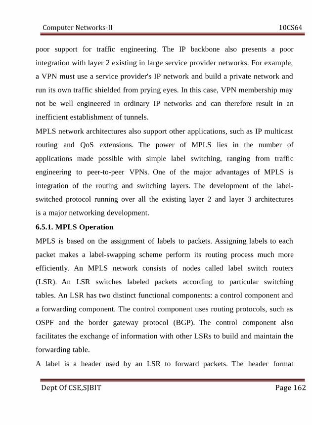
Computer Networks-II 10CS64
poor support for traffic engineering. The IP backbone also presents a poor
integration with layer 2 existing in large service provider networks. For example,
a VPN must use a service provider's IP network and build a private network and
run its own traffic shielded from prying eyes. In this case, VPN membership may
not be well engineered in ordinary IP networks and can therefore result in an
inefficient establishment of tunnels.
MPLS network architectures also support other applications, such as IP multicast
routing and QoS extensions. The power of MPLS lies in the number of
applications made possible with simple label switching, ranging from traffic
engineering to peer-to-peer VPNs. One of the major advantages of MPLS is
integration of the routing and switching layers. The development of the label-
switched protocol running over all the existing layer 2 and layer 3 architectures
is a major networking development.
6.5.1. MPLS Operation
MPLS is based on the assignment of labels to packets. Assigning labels to each
packet makes a label-swapping scheme perform its routing process much more
efficiently. An MPLS network consists of nodes called label switch routers
(LSR). An LSR switches labeled packets according to particular switching
tables. An LSR has two distinct functional components: a control component and
a forwarding component. The control component uses routing protocols, such as
OSPF and the border gateway protocol (BGP). The control component also
facilitates the exchange of information with other LSRs to build and maintain the
forwarding table.
A label is a header used by an LSR to forward packets. The header format
Dept Of CSE,SJBIT Page 162
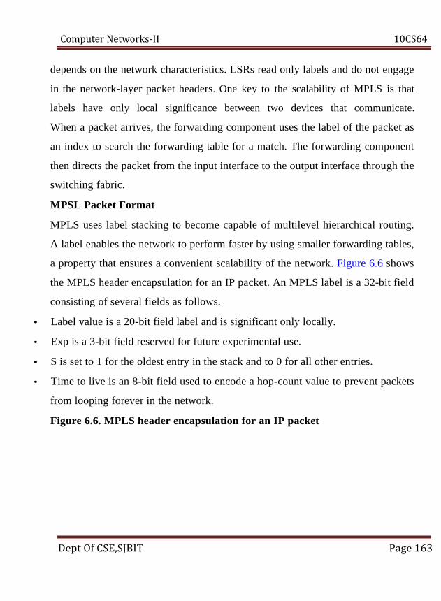
Computer Networks-II 10CS64
depends on the network characteristics. LSRs read only labels and do not engage
in the network-layer packet headers. One key to the scalability of MPLS is that
labels have only local significance between two devices that communicate.
When a packet arrives, the forwarding component uses the label of the packet as
an index to search the forwarding table for a match. The forwarding component
then directs the packet from the input interface to the output interface through the
switching fabric.
MPSL Packet Format
MPLS uses label stacking to become capable of multilevel hierarchical routing.
A label enables the network to perform faster by using smaller forwarding tables,
a property that ensures a convenient scalability of the network. Figure 6.6 shows
the MPLS header encapsulation for an IP packet. An MPLS label is a 32-bit field
consisting of several fields as follows.
• Label value is a 20-bit field label and is significant only locally.
• Exp is a 3-bit field reserved for future experimental use.
• S is set to 1 for the oldest entry in the stack and to 0 for all other entries.
• Time to live is an 8-bit field used to encode a hop-count value to prevent packets
from looping forever in the network.
Figure 6.6. MPLS header encapsulation for an IP packet
Dept Of CSE,SJBIT Page 163
Computer Networks-II 10CS64
6.5.2. Routing in MPLS Domains
Figure 6.7 shows the label-switching paradigm in an MPLS network. An ingress
LSR is an edge device that performs the initial packet processing and
classification and applies the first label. An ingress LSR creates a new label. A
core LSR swaps the incoming label with a corresponding next-hop label found
from a forwarding table. At the other end of the network, another edge router, the
egress LSR, is an outbound edge router and pops the label from the packet. It
should be noted that multiple labels may be attached to a packet, forming a stack
of labels. Label stacking enables multilevel hierarchical routing. For example,
BGP labels are used for higher-level hierarchical packet forwarding from one
BGP speaker to the other, whereas Interior Gateway Protocol (IGP) labels are
used for packet forwarding within an autonomous system. Only the label at the
top of the stack determines the forwarding decision.
Figure 6.5. Multiple layer 2 switching example in MPLS
Dept Of CSE,SJBIT Page 164

Computer Networks-II 10CS64
Once an IP packet enters an MPLS domain, the ingress LSR processes its header
information and maps that packet to a forward equivalence class (FEC). At this
point, a label switch path (LSP) through the network must be defined, and the
QoS parameters along that path must be established. The QoS parameters define
how many resources are to be used for the path and what queueing and
discarding policy are to be used. For these functions, two protocols are used to
exchange necessary information among routers: An intradomain routing
protocol, such as OSPF, is used to exchange routing information, and the Label
Distribution Protocol (LDP) assigns labels. At the end of the process, the router
appends an appropriate label for FEC purposes and forwards the packet through.
Packet forwarding at the core LSR is based on a label-swapping mechanism.
Once it receives a labeled packet, the core LSR reads the label as an index to
search in the incoming label map table for the corresponding next-hop label. The
label in the MPLS header is swapped with the out-label and sent on the next hop.
This method of packet forwarding simplifies the routing process by replacing the
longest-prefix match of IP routing with simple short-label exact-match
forwarding. The real benefit of this method is that instead of processing IP
Dept Of CSE,SJBIT Page 165
Computer Networks-II 10CS64
headers for forwarding packets, routers process a short label. Once a packet
arrives at the egress LSR, its MPLS header is decapsulated, and the stripped
packet is routed to its destination.
In summary, an MPLS domain has three label manipulation instructions: An
ingress LSR creates a new label and pushes it to the label stack of a packet, a
core LSR swaps the incoming label with a corresponding next-hop label found
from the forwarding table, and an egress LSR (outbound edge router) pops a
label from the label stack. Only the label at the top of the stack determines the
forwarding decision. The egress LSR strips the label, reads the IP packet header,
and forwards the packet to its final destination.
6.5.3. Tunneling and Use of FEC
In an MPLS operation, any traffic is grouped into FECs. FEC implies that a
group of IP packets are forwarded in the same mannerfor example, over the same
path or with the same forwarding treatment. A packet can be mapped to a
particular FEC, based on the following criteria:
• Source and/or destination IP address or IP network addresses
• TCP/UDP port numbers
• Class of service
• Applications
As mentioned earlier, labels have only local significance. This fact removes a
considerable amount of the network-management burden. An MPLS packet may
carry as many labels as required by a network sender. The process of labeled
packets can always be performed based on the top label. The feature of label
stack allows the aggregation of LSPs into a single LSP for a portion of the route,
Dept Of CSE,SJBIT Page 166

Computer Networks-II 10CS64
creating an MPLS tunnel. Figure 6.8 shows an IP packet moving through an
MPLS domain. When the labeled packet reaches the ingress LSR, each incoming
IP packet is analyzed and classified into different FECs. This traffic-
classification scheme provides the capability to partition the traffic for service
differentiation.
Figure 6.8. An IP packet labeled in an MPLS domain and tunneled to reach
the other end of the domain
Route selection can be done either hop by hop or by explicit routing. With hop-
byhop routing, each LSR can independently choose the next hop for each FEC.
Hop-byhop routing does not support traffic engineering, owing to limited
available resources. Explicit routing can provide all the benefits of traffic
engineering. With explicit routing, a single LSR determines the LSP for a given
FEC. For explicit routing, LSRs in the LSP are identified, whereas in an explicit
routing, only some of the LSRs in an LSP are specified.
With the introduction of constraint-based routing, FEC can segregate the traffic
into different levels of QoS, each with different service constraints, to support a
variety of services, such as latency-based voice traffic and security-based VPN.
At the beginning of the tunnel, an LSR assigns the same label to packets from a
Dept Of CSE,SJBIT Page 167

Computer Networks-II 10CS64
number of LSPs by pushing the label onto each packet's stack. At the other side
of the tunnel, another LSR pops the top element from the label stack, revealing
the inner label.
6.6 Overlay Networks:
An overlay network is an application-specific computer network built on top of
another network. In other words, an overlay network creates a virtual topology
on top of the physical topology. This type of network is created to protect the
existing network structure from new protocols whose testing phases require
Internet use. Such networks protect packets under test while isolating them from
the main networking infrastructure in a test bed.
Figure 6.11 shows an overlay network configured over a wide area network.
Nodes in an overlay network can be thought of as being connected by logical
links. In Figure 6.11, for example, routers R4, R5, R6, and R1 are participating in
creating an overlay network where the interconnection links are realized as
overlay logical links. Such a logical link corresponds to a path in the underlying
network. An obvious example of these networks is the peer-to-peer network,
which runs on top of the Internet. Overlay networks have no control over how
packets are routed in the underlying network between a pair of overlay
source/destination nodes. However, these networks can control a sequence of
overlay nodes through a message-passing function before reaching the
destination.
Figure 6.11. An overlay network for connections between two LANs
associated with routers R1 and R4
Dept Of CSE,SJBIT Page 168
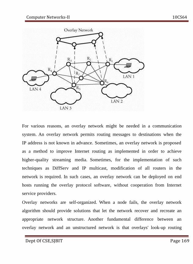
Computer Networks-II 10CS64
For various reasons, an overlay network might be needed in a communication
system. An overlay network permits routing messages to destinations when the
IP address is not known in advance. Sometimes, an overlay network is proposed
as a method to improve Internet routing as implemented in order to achieve
higher-quality streaming media. Sometimes, for the implementation of such
techniques as DiffServ and IP multicast, modification of all routers in the
network is required. In such cases, an overlay network can be deployed on end
hosts running the overlay protocol software, without cooperation from Internet
service providers.
Overlay networks are self-organized. When a node fails, the overlay network
algorithm should provide solutions that let the network recover and recreate an
appropriate network structure. Another fundamental difference between an
overlay network and an unstructured network is that overlays' look-up routing
Dept Of CSE,SJBIT Page 169

Computer Networks-II 10CS64
information is on the basis of identifiers derived from the content of moving
frames.
6.6.1. Peer-to-Peer (P2P) Connection
As an overlay network resembles a system consisting of various applications
running on a single operating system, it could also resemble a set of tunnels that
interconnect resources and users. The interconnects are carried out by peer-to-
peer (P2P) protocols.
Let δ be the time required to establish a connection and tf be the time to finish
the service as soon as the connection establishes. Assuming that the requests
arrive at random to a peer node, the service time s is
Equation 16.1
When a request arrives, the peer can be connected with probability pc and not
connected with probability 1 - pc. Realizing that s is a continuous random
variable (see Appendix C) and is discrete for its two cases, discussed in Equation
(6.1), the expected value of average service time is derived by
Equation 16.2
Let be the utilization of the peer node, where λ is the request arrival rate,
and µ is the average service rate. Thus, a fraction ρ of any given time that either
Dept Of CSE,SJBIT Page 170

Computer Networks-II 10CS64
"the peer uses for connecting' or "the connection is used for service' is expressed
by
Equation 16.3
Similarly, the fraction 1 - ρ that the same mentioned given time is idle can be
derived by
Equation 16.4
where the idle time occurs when the peer is either disconnected or connected but
not using the connection. We can now derive an expression for the peer
connection efficiency, u, as follows:
Equation 16.5
The connection efficiency of the peer can be used to determine the overall
efficiency of the P2P connection.
Dept Of CSE,SJBIT Page 171
Computer Networks-II 10CS64
UNIT - 7
Multimedia Networking: Overview of data compression, Digital
voice and compression, JPEG, MPEG, Limits of compression with
loss, Compression methods without loss, Overview of IP Telephony,
VoIP signaling protocols, Real-Time Media Transport Protocols,
Stream control Transmission Protocol (SCTP)
Dept Of CSE,SJBIT Page 172

Computer Networks-II 10CS64
UNIT - 7
MULTIMEDIA NETWORKING:
7.1 Overview of Data Compression:
The benefits of data compression in high-speed networks are obvious. Following
are those that are especially important for the compressed version of data.
• Less transmission power is required.
• Less communication bandwidth is required.
• System efficiency is increased.
There are, however, certain trade-offs with data compression. For example, the
encoding and decoding processes of data compression increase the cost,
complexity, and delay of data transmission. Both of the two processes of data
compression are required for producing multimedia networking information:
compression with loss and compression without loss.
In the first category of data compression, some less valuable or almost similar
data must be eliminated permanently. The most notable case of compression
with loss is the process of signal sampling. In this category, for example, is voice
sampling (Section 7.2). With data compression without data loss, the compressed
data can be recovered and converted back to its original form when received.
This method of compression is typically applied to digital bits after sampling.
Figure 7.1 shows the basic information process in high-speed communication
systems. Any type of "source" data is converted to digital form in a long
Dept Of CSE,SJBIT Page 173
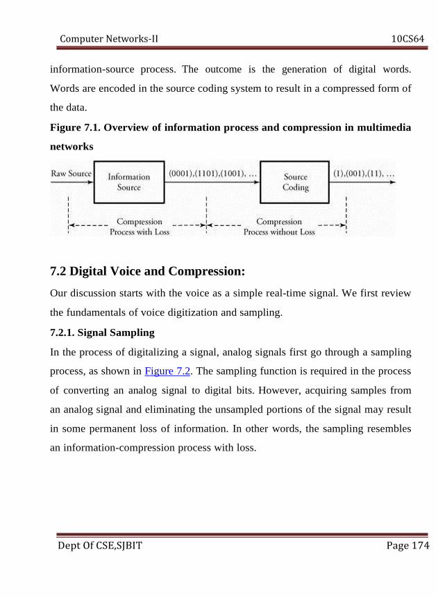
Computer Networks-II 10CS64
information-source process. The outcome is the generation of digital words.
Words are encoded in the source coding system to result in a compressed form of
the data.
Figure 7.1. Overview of information process and compression in multimedia
networks
7.2 Digital Voice and Compression:
Our discussion starts with the voice as a simple real-time signal. We first review
the fundamentals of voice digitization and sampling.
7.2.1. Signal Sampling
In the process of digitalizing a signal, analog signals first go through a sampling
process, as shown in Figure 7.2. The sampling function is required in the process
of converting an analog signal to digital bits. However, acquiring samples from
an analog signal and eliminating the unsampled portions of the signal may result
in some permanent loss of information. In other words, the sampling resembles
an information-compression process with loss.
Dept Of CSE,SJBIT Page 174

Computer Networks-II 10CS64
Figure 7.2. Overview of digital voice process
Sampling techniques are of several types:
• Pulse amplitude modulation (PAM), which translates sampled values to pulses
with corresponding amplitudes
• Pulse width modulation (PWM), which translates sampled values to pulses with
corresponding widths
• Pulse position modulation (PPM), which translates sampled values to identical
pulses but with corresponding positions to sampling points
PAM is a practical and commonly used sampling method; PPM is the best
modulation technique but is expensive. PWM is normally used in analog remote-
control systems. The sampling rate in any of these schemes obeys the Nyquist
theorem, according to which at least two samples on all components of the
spectrum are needed in order to reconstruct a spectrum:
Equation 17.1
where fH is the highest-frequency component of a signal, and fS is the sampling
Dept Of CSE,SJBIT Page 175

Computer Networks-II 10CS64
rate.
7.2.2. Quantization and Distortion
Samples are real numbersdecimal-point values and integer valuesand, thus, up to
infinite bits are required for transmission of a raw sample. The transmission of
infinite bits occupies infinite bandwidth and is not practical for implementation.
In practice, sampled values are rounded off to available quantized levels.
However, rounding off the values loses data and generates distortion. A measure
is needed to analyze this distortion. The distortion measure should show how far
apart a signal denoted by x(t) is to its reproduced version, denoted by . The
distortion measure of a single source is the difference between source sample Xi
and its corresponding quantized value , denoted by , and is widely
known as squared-error distortion:
Equation 17.2
Note that is noninvertible, since lost information cannot be recovered. The
distortion measure of n samples is based on the values of source samples
obtained at the sampler output. As a result, the collection of n samples forms a
random process:
Equation 17.3
Dept Of CSE,SJBIT Page 176

Computer Networks-II 10CS64
Similarly, the reconstructed signal at the receiver can be viewed as a random
process:
Equation 17.4
The distortion between these two sequences is the average between their
components:
Equation 17.5
Note that itself is a random variable, since it takes on random
numbers. Thus, the total distortion between the two sequences is defined as the
expected value of :
Equation 17.6
If all samples are expected to have approximately the same distortion denoted by
Dept Of CSE,SJBIT Page 177
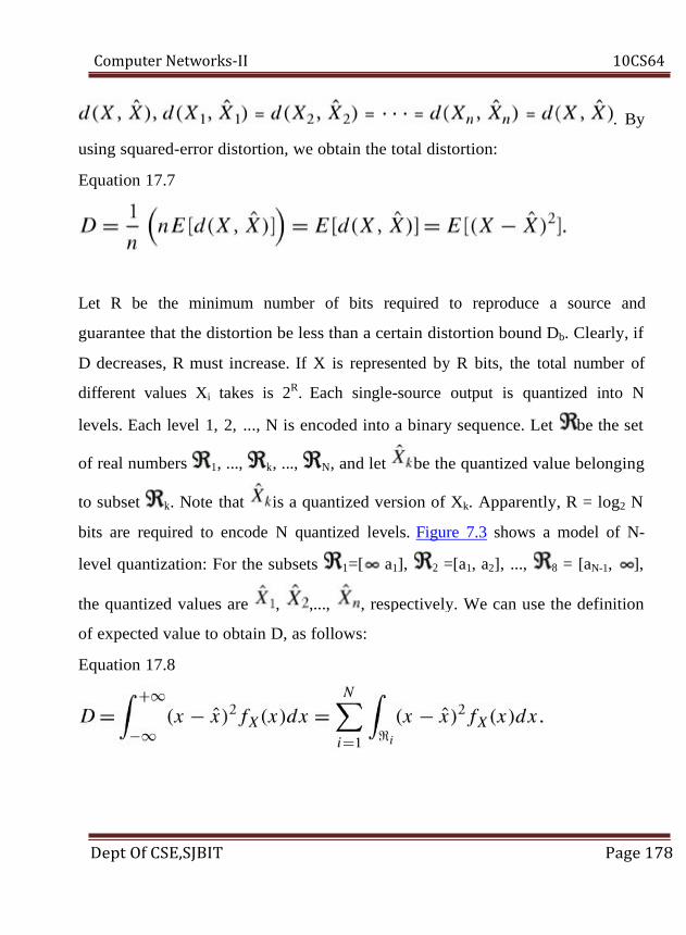
Computer Networks-II 10CS64
. By
using squared-error distortion, we obtain the total distortion:
Equation 17.7
Let R be the minimum number of bits required to reproduce a source and
guarantee that the distortion be less than a certain distortion bound Db. Clearly, if
D decreases, R must increase. If X is represented by R bits, the total number of
different values Xi takes is 2R. Each single-source output is quantized into N
levels. Each level 1, 2, ..., N is encoded into a binary sequence. Let be the set
, and let be the quantized value belonging
. Note that is a quantized version of Xk. Apparently, R = log2 N
bits are required to encode N quantized levels. Figure 7.3 shows a model of N-
level quantization: For the subsets
the quantized values are , ,...,
of expected value to obtain D, as follows:
Equation 17.8
Dept Of CSE,SJBIT Page 178
k N , ..., 1 of real numbers , ...,
to subset k
=[ a1], 1 =[a1, a2], ..., 2 = [aN-1, ], 8
, respectively. We can use the definition

Computer Networks-II 10CS64
Figure 7.3. N-level quantization
Typically, a distortion bound denoted by Db is defined by designers to ensure
that Db D.
Dept Of CSE,SJBIT Page 179
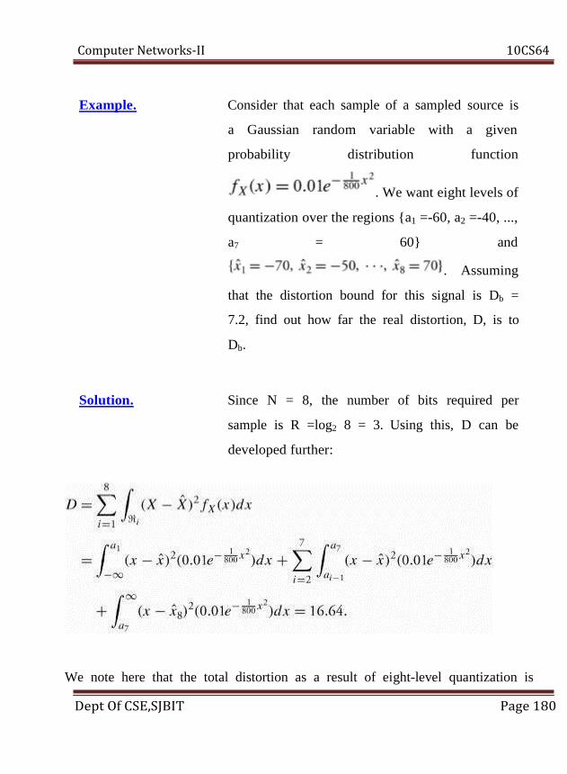
Computer Networks-II 10CS64
Example. Consider that each sample of a sampled source is
a Gaussian random variable with a given
probability distribution function
. We want eight levels of
quantization over the regions {a1 =-60, a2 =-40, ...,
a7 = 60} and
. Assuming
that the distortion bound for this signal is Db =
7.2, find out how far the real distortion, D, is to
Db.
Solution. Since N = 8, the number of bits required per
sample is R =log2 8 = 3. Using this, D can be
developed further:
We note here that the total distortion as a result of eight-level quantization is
Dept Of CSE,SJBIT Page 180

Computer Networks-II 10CS64
16.64, which is considerably greater than the given distortion bound of 7.2.
The conclusion in the example implies that the quantization chosen for that
source may not be optimal. A possible reason may be inappropriate choices of
(a1, ..., a7) and/or . This in turn means that R is not optimal.
Optimal Quantizers
Let Δ be the length of each region equal to ai+1 - ai. Thus, regions can be restated
as ( - , a1) ... (aN-1, + ). Clearly, the limits of the upper region can also be
shown by (a1 + (N - 2)Δ, + ). Then, the total distortion can be rewritten as
Equation 17.9
For D to be optimized, we must have , and also , ...,
.
The resu1t of solving the N + 2 equations can be summarized as follows. For N =
even:
Equation 17.10
and
Dept Of CSE,SJBIT Page 181

Computer Networks-II 10CS64
Equation 7.11
For N = odd:
Equation 7.12
and
Equation 7.13
7.3 JPEG & MPEG Files:
Color images are based on the fact that any color can be represented to the
human eye by using a particular combination of the base colors red, green, and
blue (RGB). Computer monitor screens, digital camera images, or any other still
color images are formed by varying the intensity of the three primary colors at
pixel level, resulting in the creation of virtually any corresponding color from the
real raw image. Each intensity created on any of the three pixels is represented
by 8 bits, as shown in Figure 17.6. The intensities of each 3-unit pixel are
adjusted, affecting the value of the 8-bit word to produce the desired color. Thus,
each pixel can be represented by using 24 bits, allowing 224 different colors.
However, the human eye cannot distinguish all colors among the 224 possible
Dept Of CSE,SJBIT Page 182

Computer Networks-II 10CS64
colors. The number of pixels in a typical image varies with the image size.
GIF Files
JPEG is designed to work with full-color images up to 224 colors. The graphics
interchange format (GIF) is an image file format that reduces the number of
colors to 256. This reduction in the number of possible colors is a trade-off
between the quality of the image and the transmission bandwidth. GIF stores up
to 28 = 256 colors in a table and covers the range of colors in an image as closely
as possible. Therefore, 8 bits are used to represent a single pixel. GIF uses a
variation of Lempel-Ziv encoding (Section 17.6.3) for compression of an image.
This technology is used for images whose color detailing is not important, such
as cartoons and charts.
DCT Process
The discrete cosine transform (DCT) is a lossy compression process that begins
by dividing a raw image into a series of standard N x N pixel blocks. For now,
consider a monochrome block of pixels. With a standard size of N = 8, N is the
number of pixels per row or column of each block. Let x, y be the position of a
particular pixel in a block where 0 x N - 1 and 0 y N - 1. Hence, a gray
scale of a given pixel x, y can get an integer value in {0, 1, 2, ..., 255}. For an N
x N pixel block, the DCT process is summarized in two steps
1. Form a P[x][y] matrix to represent the collection of light-
intensity values taken from various points of a real raw image.
Dept Of CSE,SJBIT Page 183

Computer Networks-II 10CS64
2. Convert the values of P[x][y]matrix to matrix with normalized
and reduced values denoted by T[i][j] obtained as follows.
The objective of matrix T[i][j] is to create as many 0s as possible instead of
small numbers in the P[x][y] matrix in order to reduce the overall bandwidth
required to transmit the image. Similarly, matrix T[i][j] is a two-dimensional
array with N rows and N columns, where 0 i N - 1 and 0 j N - 1. The
elements of T[i][j] are known as spatial frequencies and are obtained from
Equation 17.14
where
Moving Images and MPEG Compression
A motion image, or video is a rapid display of still images. Moving from one
image to another must be fast enough to fool the human eye. There are different
standards on the number of still images comprising a video clip. One common
standard produces a motion image by displaying still images at a rate of 30
frames per second. The common standard that defines the video compression is
the Moving Pictures Expert Group (MPEG), which has several branch standards:
Dept Of CSE,SJBIT Page 184

Computer Networks-II 10CS64
• MPEG-1, primarily for video on CD-ROM
• MPEG-2, for multimedia entertainment and high-definition television (HDTV)
and the satellite broadcasting industry
• MPEG-4, for object-oriented video compression and videoconferencing over
low-bandwidth channels
• MPEG-7, for a broad range of demands requiring large bandwidths providing
multimedia tools
• MPEG-21 for interaction among the various MPEG groups
Logically, using JPEG compression for each still picture does not provide
sufficient compression for video as it occupies a large bandwidth. MPEG
deploys additional compression. Normally, the difference between two
consecutive frames is small. With MPEG, a base frame is sent first, and
successive frames are encoded by computing the differences. The receiver can
reconstruct frames based on the first base frame and the submitted differences.
However, frames of a completely new scene in a video may not be compressed
this way, as the difference between the two scenes is substantial. Depending on
the relative position of a frame in a sequence, it can be compressed through one
of the following types of frames:
• Interimage (I) frames. An I frame is treated as a JPEG still image and
compressed using DCT.
• Predictive (P) frames. These frames are produced by computing differences
between a current and a previous I or P frame.
• Bidirectional (B) frames. A B frame is similar to a P frame, but the P frame
considers differences between a previous, current, and future frames.
Dept Of CSE,SJBIT Page 185

Computer Networks-II 10CS64
Figure 7.9 illustrates a typical grouping of frames, with I, P, and B frames
forming a sequence. In any frame sequence, I frames appear periodically as the
base of the scene. Normally, there is a P frame between each two groups of B
frames.
Figure 7.9. Snapshot of moving frames for MPEG compression
7.4.1. MP3 and Streaming Audio
Section 7.2 explained how an audible sound or a human voice ranging between
20 Hz and 20 KHz can be converted into digital bits and eventually into packets
for networking. A signal is sampled, quantized, and encoded, a process called
PCM. A variety of methods of compressing such encoded products at the output
of the PCM are available. However, Huffman compression of the processed
signal may not be sufficient for transmission over IP networks.
The MPEG-1 layer 3 (MP3) technology compresses audio for networking and
Dept Of CSE,SJBIT Page 186

Computer Networks-II 10CS64
producing CD-quality sound. The sampling part of PCM is performed at a rate of
44.1 KHz to cover the maximum of 20 KHz of audible signals. Using the
commonly used 16-bit encoding for each sample, the maximum total bits
required for audio is 16 x 44.1 = 700 kilobits and 1.4 megabits for two channels
if the sound is processed in a stereo fashion. For example a 60-minute CD (3,600
seconds) requires about 1.4 x 3,600 = 5,040 megabits, or 630 megabytes. This
amount may be acceptable for recording on a CD but is considered extremely
large for networking, and thus a carefully designed compression technique is
needed.
MP3 combines the advantages of MPEG with "three" layers of audio
compressions. MP3 removes from a piece of sound all portions that an average
ear may not be able to hear, such as weak background sounds. On any audio
streaming, MP3 specifies what humans are not able to hear, removes those
components, and digitizes the remaining. By filtering some part of an audio
signal, the quality of compressed MP3 is obviously degraded to lower than the
original one. Nonetheless, the compression achievement of this technology is
remarkable.
7.4 Limits of Compression with Loss:
Hartely, Nyquist, and Shannon are the founders of information theory,
which has resulted in the mathematical modeling of information sources.
Consider a communication system in which a source signal is processed to
produce sequences of n words, as shown in Figure 7.10. These sequences of
digital bits at the output of the information source can be compressed in the
Dept Of CSE,SJBIT Page 187
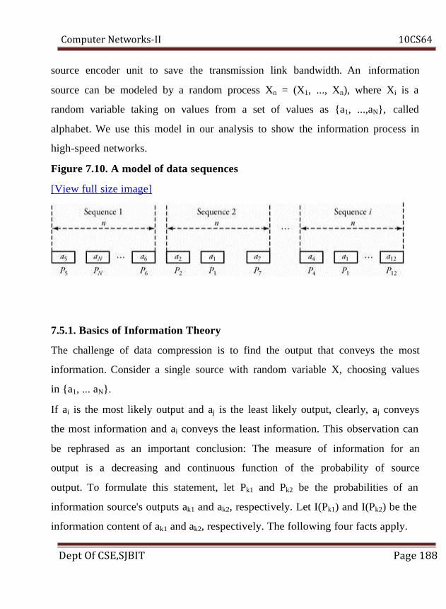
Computer Networks-II 10CS64
source encoder unit to save the transmission link bandwidth. An information
source can be modeled by a random process Xn = (X1, ..., Xn), where Xi is a
random variable taking on values from a set of values as {a1, ...,aN}, called
alphabet. We use this model in our analysis to show the information process in
high-speed networks.
Figure 7.10. A model of data sequences
[View full size image]
7.5.1. Basics of Information Theory
The challenge of data compression is to find the output that conveys the most
information. Consider a single source with random variable X, choosing values
in {a1, ... aN}.
If ai is the most likely output and aj is the least likely output, clearly, aj conveys
the most information and ai conveys the least information. This observation can
be rephrased as an important conclusion: The measure of information for an
output is a decreasing and continuous function of the probability of source
output. To formulate this statement, let Pk1 and Pk2 be the probabilities of an
information source's outputs ak1 and ak2, respectively. Let I(Pk1) and I(Pk2) be the
information content of ak1 and ak2, respectively. The following four facts apply.
Dept Of CSE,SJBIT Page 188

Computer Networks-II 10CS64
1. As discussed, I(Pk) depends on Pk.
2. I(Pk) = a continuous function of Pk.
3. I(Pk) = a decreasing function of Pk.
4. Pk = Pk1.Pk2 (probability of two outputs happen in the same time).
5. I(Pk) = I(Pk1) + I(Pk2) (sum of two pieces of information).
These facts lead to an important conclusion that can relate the probability of a
certain data to its information content:
Equation 17.16
The log function has a base 2, an indication of incorporating the binary concept
of digital data.
7.4.2. Entropy of Information
In general, entropy is a measure of uncertainty. Consider an information source
producing random numbers, X, from a possible collection of {a1, ..., aN} with
corresponding probabilities of {P1,...,PN} and information content of {I (P1),..., I
(PN)}, respectively. In particular, the entropy, H(x), is defined as the average
information content of a source:
Equation 17.17
Dept Of CSE,SJBIT Page 189

Computer Networks-II 10CS64
Example. A source with bandwidth 8 KHz is sampled at the
Nyquist rate. If the result is modeled using any
value from {-2,-1,0,1,2} and corresponding
probabilities {0.05, 0.05, 0.08, 0.30, 0.52}, find
the entropy.
Solution.
The information rate in samples/sec = 8,000 x 2 = 16,000, and the rate of
information produced by the source = 16,000 x 0.522 = 8,352 bits.
Joint Entropy
The joint entropy of two discrete random variables X and Y is defined by
Equation 17.18
where PX,Y (x, y) = Prob[X = x and the same time Y = y] and is called the joint
probability mass function of two random variables. In general, for a random
process Xn = (X1,..., Xn) with n random variables:
Equation 17.19
Dept Of CSE,SJBIT Page 190

Computer Networks-II 10CS64
where PX1, ..., Xn (x1, ...., xn) is the joint probability mass function (J-PMF) of the
random process Xn. For more information on J-PMF,
7.4.3. Shannon's Coding Theorem
This theorem limits the rate of data compression. Consider again Figure 7.10,
which shows a discrete source modeled by a random process that generates
sequences of length n using values in set {a1, ..., aN} with probabilities {P1, ...,
PN}, respectively. If n is large enough, the number of times a value ai is repeated
in a given sequence = nPi, and the number of values in a typical sequence is
therefore n(P1 +... + PN).
We define the typical sequence as one in which any value ai is repeated nPi
times. Accordingly, the probability that ai is repeated nPi times is obviously
, resulting in a more general statement: The probability of a
typical sequence is the probability [(a1 is repeated np1)] x the probability [(a2 is
repeated np2] x .... This can be shown by , or
Equation 17.20
Knowing , we can obtain the probability of a typical
Dept Of CSE,SJBIT Page 191

Computer Networks-II 10CS64
sequence Pt as follow:
Equation 17.21
This last expression results in the well-known Shannon's theorem, which
expresses the probability that a typical sequence of length n with entropy HX(x)
is equal to
Equation 17.22
Example. Assume that a sequence size of 200 of an
information source chooses values from the set
{a1, ..., a5} with corresponding probabilities {0.05,
0.05, 0.08, 0.30, 0.52}. Find the probability of a
typical sequence.
Solution. In the previous example, we calculated the
Dept Of CSE,SJBIT Page 192

Computer Networks-II 10CS64
entropy to be HX(x) = 0.522 for the same
situation. With n = 200, N = 5, the probability of a
typical sequence is the probability of a sequence
in which a1, a2, a3, a4, and a5 are repeated,
respectively, 200 x 0.05 = 10 times, 10 times, 16
times, 60 times, and 104 times. Thus, the
probability of a typical sequence is Pt = 2-nH (x) =
2-200(0.52).
The fundamental Shannon's theorem leads to an important conclusion. As the
probability of a typical sequence is 2-nHX(x) and the sum of probabilities of all
typical sequences is 1, the number of typical sequences is obtained by
.
Knowing that the total number of all sequences, including typical and nontypical
ones, is Nn, it is sufficient, in all practical cases when n is large enough, to
transmit only the set of typical sequences rather than the set of all sequences.
This is the essence of data compression: The total number of bits required to
represent 2nHX(x) sequences is nHX(x) bits, and the average number of bits for
each source = HX(x).
Following the previous example, in which the
sequence size for an information source is 200,
find the ratio of the number of typical sequences
to the number of all types of sequences.
Page 193
X
Example.
Dept Of CSE,SJBIT
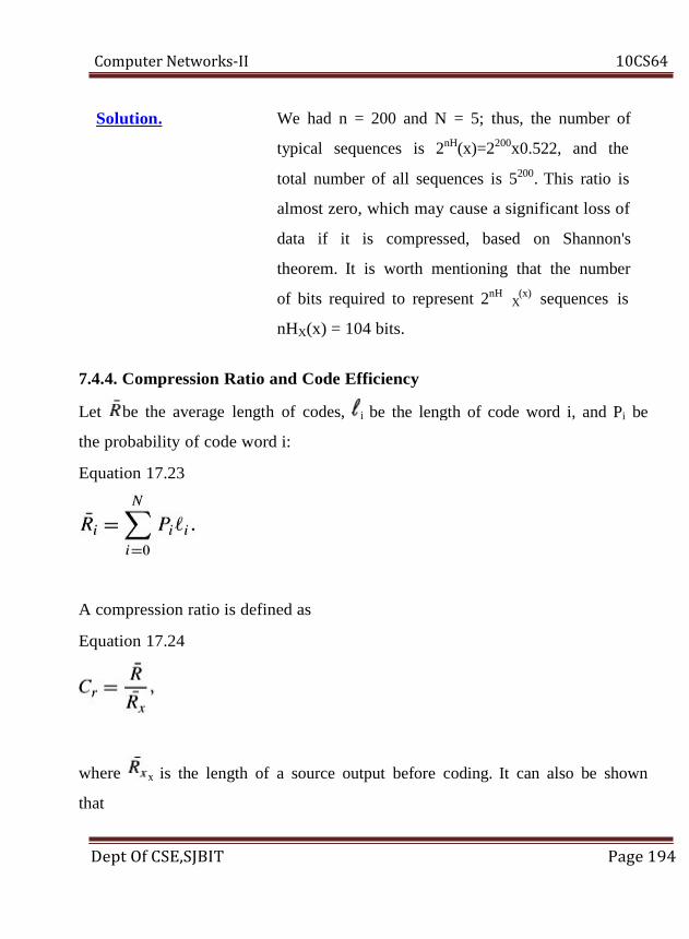
10CS64
We had n = 200 and N = 5; thus, the number of
typical sequences is 2nH(x)=2200x0.522, and the
total number of all sequences is 5200. This ratio is
almost zero, which may cause a significant loss of
data if it is compressed, based on Shannon's
theorem. It is worth mentioning that the number
of bits required to represent 2nH (x) sequences is
nHX(x) = 104 bits.
7.4.4. Compression Ratio and Code Efficiency
Let be the average length of codes,
the probability of code word i:
Equation 17.23
A compression ratio is defined as
Equation 17.24
is the length of a source output before coding. It can also be shown
that
Dept Of CSE,SJBIT Page 194
Computer Networks-II
Solution.
X
be the length of code word i, and Pi be i
where x

Computer Networks-II 10CS64
Equation 7.25
Code efficiency is a measure for understanding how close code lengths are to the
corresponding decoded data and is defined by
Equation 7.26
When data is compressed, part of the data may need to be removed in the
process.
7.5 Compression Methods Without Loss:
Some types of data, including text, image, and video, might contain redundant or
repeated elements. If so, those elements can be eliminated and some sort of
codes substituted for future decoding. In this section, we focus on techniques that
do not incur any loss during compression:
• Arithmetic encoding
• Run-length encoding
• Huffman encoding
• Lempel-Ziv encoding
Here, we ignore arithmetic encoding and consider only the last three encoding
Dept Of CSE,SJBIT Page 195

Computer Networks-II 10CS64
techniques.
7.5.1. Run-Length Encoding
One of the simplest data-compression techniques is run-length encoding. This
technique is fairly effective for compression of plaintext and numbers, especially
for facsimile systems. With run-length code, repeated letters can be replaced by a
run length, beginning with Cc to express the compression letter count.
7.7 Overview of IP Telephony:
An IP telephone can be used to make telephone calls over IP networks.
Voice over IP (VoIP), or IP telephony, uses packet-switched networks to carry
voice traffic in addition to data traffic. The basic scheme of IP telephony starts
with pulse code modulation, discussed in Chapter 7. The encoded data is
transmitted as packets over packet-switched networks. At a receiver, the data is
decoded and converted back to analog form. The packet size must be properly
chosen to prevent large delays. The IP telephone system must also be able to
handle the signaling function of the call setup, mapping of phone number to IP
address, and proper call termination.
Basic components of an IP telephone system include IP telephones, the Internet
backbone, and signaling servers, as shown in Figure 7.1. The IP telephone can
also be a laptop or a computer with the appropriate software. An IP telephone
connects to the Internet through a wired or a wireless medium. The signaling
servers in each domain are analogous to the central processing unit in a computer
and are responsible for the coordination between IP phones. The hardware
devices required to deploy packet-switched networks are less expensive than
Dept Of CSE,SJBIT Page 196

Computer Networks-II 10CS64
those required for the connection-oriented public-switched telephone networks.
On a VoIP network, network resources are shared between voice and data traffic,
resulting in some savings and efficient use of the available network resources.
Figure 7.1. Voice over IP system
A VoIP network is operated through two sets of protocols: signaling protocols
and real-time packet-transport protocols. Signaling protocols handle call setups
and are controlled by the signaling servers. Once a connection is set, RTP
transfers voice data in real-time fashion to destinations. RTP runs over UDP
because TCP has a very high overhead. RTP builds some reliability into the UDP
scheme and contains a sequence number and a real-time clock value. The
sequence number helps RTP recover packets from out-of-order delivery. Two
RTP sessions are associated with each phone conversation. Thus, the IP
telephone plays a dual role: an RTP sender for outgoing data and an RTP
Dept Of CSE,SJBIT Page 197
Computer Networks-II 10CS64
receiver for incoming data.
7.1.1. VoIP Quality-of-Service
A common issue that affects the QoS of packetized audio is jitter. Voice
data requires a constant packet interarrival rate at receivers to convert data into a
proper analog signal for playback. The variations in the packet interarrival rate
lead to jitter, which results in improper signal reconstruction at the receiver.
Typically, an unstable sine wave reproduced at the receiver results from the jitter
in the signal. Buffering packets can help control the interarrival rate. The
buffering scheme can be used to output the data packets at a fixed rate. The
buffering scheme works well when the arrival time of the next packet is not very
long. Buffering can also introduce a certain amount of delay.
Another issue having a great impact on real-time transmission quality is
network latency, or delay, which is a measure of the time required for a data
packet to travel from a sender to a receiver. For telephone networks, a round-trip
delay that is too large can result in an echo in the earpiece. Delay can be
controlled in networks by assigning a higher priority for voice packets. In such
cases, routers and intermediate switches in the network transport these high-
priority packets before processing lower-priority data packets.
Congestion in networks can be a major disruption for IP telephony.
Congestion can be controlled to a certain extent by implementing weighted
random early discard, whereby routers begin to intelligently discard lower-
priority packets before congestion occurs. The drop in packets results in a
subsequent decrease in the window size in TCP, which relieves congestion to a
certain extent.
Dept Of CSE,SJBIT Page 198

Computer Networks-II 10CS64
A VoIP connection has several QoS factors:
• Packet loss is accepted to a certain extent.
• Packet delay is normally unacceptable.
• Jitter, as the variation in packet arrival time, is not acceptable after a certain
limit.
Packet loss is a direct result of the queueing scheme used in routers. VoIP can
use priority queueing, weighted fair queuing, or class-based weighted fair
queuing, whereby traffic amounts are also assigned to classes of data traffic.
Besides these well-known queueing schemes, voice traffic can be handled by a
custom queuing, in which a certain amount of channel bandwidth for voice
traffic is reserved.
Although the packet loss is tolerable to a certain extent, packet delay may not be
tolerable in most cases. The variability in the time of arrival of packets in packet-
switched networks gives rise to jitter variations. This and other QoS issues have
to be handled differently than in conventional packet-switched networks. QoS
must also consider connectivity of packet-voice environment when it is
combined with traditional telephone networks.
7.6.2. VoIP Signaling Protocols
The IP telephone system must be able to handle signalings for call setup,
conversion of phone number to IP address mapping, and proper call termination.
Signaling is required for call setup, call management, and call termination. In the
standard telephone network, signaling involves identifying the user's location
Dept Of CSE,SJBIT Page 199

Computer Networks-II 10CS64
given a phone number, finding a route between a calling and a called party, and
handling the issue of call forwarding and other call features.
IP telephone systems can use either a distributed or a centralized signaling
scheme. The distributed approach enables two IP telephones to communicate
using a client/ server model, as most Internet applications do. The distributed
approach works well with VoIP networks within a single company. The
centralized approach uses the conventional model and can provide some level of
guarantee. Three well-known signaling protocols are
1. Session Initiation Protocol (SIP)
2. H.323 protocols
3. Media Gateway Control Protocol (MGCP)
Figure 7.2 shows the placement of VoIP in the five-layer TCP/IP model. SIP,
H.323, and MGCP run over TCP or UDP; real-time data transmission protocols,
such as RTP, typically run over UDP. Real-time transmissions of audio and
video traffic are implemented over UDP, since the real-time data requires lower
delay and less overhead. Our focus in this chapter is on the two signaling
protocols SIP and H.323 and on RTP and RTCP.
Figure 7.2. Main protocols for VoIP and corresponding layers of operation
Dept Of CSE,SJBIT Page 200

Computer Networks-II 10CS64
7.2.1. Session Initiation Protocol (SIP)
The Session Initiation Protocol (SIP) is one of the most important VoIP signaling
protocols operating in the application layer in the five-layer TCP/IP model. SIP
can perform both unicast and multicast sessions and supports user mobility. SIP
handles signals and identifies user location, call setup, call termination, and busy
signals. SIP can use multicast to support conference calls and uses the Session
Description Protocol (SDP) to negotiate parameters.
SIP Components
Figure 7.3 shows an overview of SIP. A call is initiated from a user agent: the
user's IP telephone system, which is similar to a conventional phone. A user
agent assists in initiating or terminating a phone call in VoIP networks. A user
agent can be implemented in a standard telephone or in a laptop with a
microphone that runs some software. A user agent is identified using its
Dept Of CSE,SJBIT Page 201

Computer Networks-II 10CS64
associated domain. For example, [email protected] refers to user 1, who is
associated with the domain1.com network.
Figure 7.3. Overview of SIP
7.3. Real-Time Media Transport Protocols
In real-time applications, a stream of data is sent at a constant rate. This data
must be delivered to the appropriate application on the destination system, using
real-time protocols. The most widely applied protocol for real-time transmission
is the Real-Time Transport Protocol (RTP), including its companion version:
Real-Time Control Protocol (RTCP).
UDP cannot provide any timing information. RTP is built on top of the existing
UDP stack. Problems with using TCP for real-time applications can be identified
easily. Real-time applications may use multicasting for data delivery. As an end-
toend protocol, TCP is not suited for multicast distribution. TCP uses a
retransmission strategy for lost packets, which then arrive out of order. Real-time
applications cannot afford these delays. TCP does not maintain timing
information for packets. In real-time applications, this would be a requirement.
Dept Of CSE,SJBIT Page 202
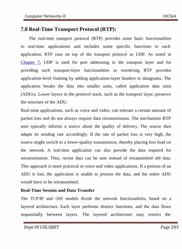
Computer Networks-II 10CS64
7.8 Real-Time Transport Protocol (RTP):
The real-time transport protocol (RTP) provides some basic functionalities
to real-time applications and includes some specific functions to each
application. RTP runs on top of the transport protocol as UDP. As noted in
Chapter 7, UDP is used for port addressing in the transport layer and for
providing such transport-layer functionalities as reordering. RTP provides
application-level framing by adding application-layer headers to datagrams. The
application breaks the data into smaller units, called application data units
(ADUs). Lower layers in the protocol stack, such as the transport layer, preserve
the structure of the ADU.
Real-time applications, such as voice and video, can tolerate a certain amount of
packet loss and do not always require data retransmission. The mechanism RTP
uses typically informs a source about the quality of delivery. The source then
adapts its sending rate accordingly. If the rate of packet loss is very high, the
source might switch to a lower-quality transmission, thereby placing less load on
the network. A real-time application can also provide the data required for
retransmission. Thus, recent data can be sent instead of retransmitted old data.
This approach is more practical in voice and video applications. If a portion of an
ADU is lost, the application is unable to process the data, and the entire ADU
would have to be retransmitted.
Real-Time Session and Data Transfer
The TCP/IP and OSI models divide the network functionalities, based on a
layered architecture. Each layer performs distinct functions, and the data flows
sequentially between layers. The layered architecture may restrict the
Dept Of CSE,SJBIT Page 203

Computer Networks-II 10CS64
implementation on certain functions out of the layered order. Integrated layer
processing dictates a tighter coupling among layers. RTP is used to transfer data
among sessions in real time. A session is a logical connection between an active
client and an active server and is defined by the following entities:
• RTP port number, which represents the destination port address of the RTP
session. Since RTP runs over UDP, the destination port address is available on
the UDP header.
• IP address of the RTP entity, which involves an RTP session. This address can
be either a unicast or a multicast address.
RTP uses two relays for data transmission. A relay is an intermediate system that
acts as both a sender and a receiver. Suppose that two systems are separated by a
firewall that prevents them from direct communication. A relay in this context is
used to handle data flow between the two systems. A relay can also be used to
convert the data format from a system into a form that the other system can
process easily. Relays are of two types: mixer and translator.
A mixer relay is an RTP relay that combines the data from two or more RTP
entities into a single stream of data. A mixer can either retain or change the data
format. The mixer provides timing information for the combined stream of data
and acts as the source of timing synchronization. Mixers can be used to combine
audio streams in real-time applications and can be used to service systems that
may not be able to handle multiple RTP streams.
The translator is a device that generates one or more RTP packets for each
incoming RTP packet. The format of the outgoing packet may be different from
that of the incoming packet. A translator relay can be used in video applications
Dept Of CSE,SJBIT Page 204

Computer Networks-II 10CS64
in which a high-quality video signal is converted to a lower-quality in order to
service receivers that support a lower data rate. Such a relay can also be used to
transfer packets between RTP entities separated by an application-level firewall.
Translators can sometimes be used to transfer an incoming multicast packet to
multiple destinations.
RTP Packet Header
RTP contains a fixed header and an application-specific variable-length header
field. Figure 7.8 shows the RTP header format. The RTP header fields are:
• Version (V), a 2-bit field indicating the protocol version.
• Padding (P), a 1-bit field that indicates the existence of a padding field at the end
of the payload. Padding is required in applications that require the payload to be
a multiple of some length.
• Extension (X), a 1-bit field indicating the use of an extension header for RTP.
• Contributing source count (CSC), a 4-bit field that indicates the number of
contributing source identifiers.
• Marker (M), a 1-bit field indicating boundaries in a stream of data traffic. For
video applications, this field can be used to indicate the end of a frame.
• Payload type, A 7-bit field specifying the type of RTP payload. This field also
contains information on the use of compression or encryption.
• Sequence number, a 16-bit field that a sender uses to identify a particular packet
within a sequence of packets. This field is used to detect packet loss and for
packet reordering.
• Timestamp, a 32-bit field enabling the receiver to recover timing information.
This field indicates the timestamp when the first byte of data in the payload was
Dept Of CSE,SJBIT Page 205
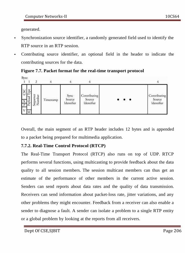
Computer Networks-II 10CS64
generated.
• Synchronization source identifier, a randomly generated field used to identify the
RTP source in an RTP session.
• Contributing source identifier, an optional field in the header to indicate the
contributing sources for the data.
Figure 7.7. Packet format for the real-time transport protocol
Overall, the main segment of an RTP header includes 12 bytes and is appended
to a packet being prepared for multimedia application.
7.7.2. Real-Time Control Protocol (RTCP)
The Real-Time Transport Protocol (RTCP) also runs on top of UDP. RTCP
performs several functions, using multicasting to provide feedback about the data
quality to all session members. The session multicast members can thus get an
estimate of the performance of other members in the current active session.
Senders can send reports about data rates and the quality of data transmission.
Receivers can send information about packet-loss rate, jitter variations, and any
other problems they might encounter. Feedback from a receiver can also enable a
sender to diagnose a fault. A sender can isolate a problem to a single RTP entity
or a global problem by looking at the reports from all receivers.
Dept Of CSE,SJBIT Page 206

Computer Networks-II 10CS64
RTCP performs source identification. RTCP packets contain some information
to identify the source of the control packet. The rate of RTCP packets must also
be kept to less than 5 percent of the total session traffic. Thus, this protocol
carries out "rate control" of RTCP packets. At the same time, all session
members must be able to evaluate the performance of all other session members.
As the number of active members in a session increases, the transmission rates of
the control packets must be reduced. RTCP is also responsible for session control
and can provide some session-control information, if necessary.
Packet Type and Format
RTCP transmits control information by combining a number of RTCP packets in
a single UDP datagram. The RTCP packet types are sender reports (SR), receiver
reports (RR), source descriptor (SDES), goodbye (BYE), and application-
specific types. Figure 7.9 shows some RTCP packet formats. The fields common
to all packet types are as follows:
• Version, a 2-bit field that indicates the current version.
• Padding, a 1-bit field that indicates the existence of padding bytes at the end of
the control data.
• Count, a 5-bit field that indicates the number of SR or RR reports or the number
of source items in the SDES packet.
• Packet type, an 8-bit field that indicates the type of RTCP packet. (Four RTCP
packet types were specified earlier.)
• Length, a 16-bit field that represents the length of packet in 32-bit words minus
1.
• Synchronization source identifier, a field common to the SR and RR packet
Dept Of CSE,SJBIT Page 207

Computer Networks-II 10CS64
types; it indicates the source of the RTCP packets.
Figure 7.9. Format of the SR packet in RCTP
Figure 7.9 also shows a typical format of a sender report. The report consists of
the common header fields and a block of sender information. The sender report
may also contain zero or more receiver report blocks, as shown in the figure. The
fields in the sender information block are:
• NTP timestamp, a 64-bit field that indicates when a sender report was sent. The
sender can use this field in combination with the timestamp field returned in
receiver reports to estimate the round-trip delay to receivers.
• RTP timestamp, a 32-bit field used by a receiver to sequence RTP data packets
from a particular source.
• Sender's packet count, a 32-bit field that represents the number of RTP data
packets transmitted by the sender in the current session.
Dept Of CSE,SJBIT Page 208

Computer Networks-II 10CS64
• Sender's byte count, a 32-bit field that represents the number of RTP data octets
transmitted by the sender in the current session.
The SR packet includes zeros or more RR blocks. One receiver block is included
for each sender from which the member has received data during the session.
The RR block includes the following fields:
• SSRC_n, a 32-bit field that identifies the source in the report block, where n is
the number of sources.
• Fraction lost, an 8-bit field indicating the fraction of data packet loss from source
SSRC_n since the last SR or RR report was sent.
• Cumulative number of packets lost, a 24-bit field that represents the total number
of RTP data packets lost from the source in the current active session identified
by SSRC_n.
• Extended highest sequence number received, the first 16 least-significant bits,
used to indicate the highest sequence number for packets received from source
SSRC_n. The first 16 most-significant bits indicate the number of times that the
sequence number has been wrapped back to zero.
• Interarrival jitter, a 32-bit field used to indicate the jitter variations at the receiver
for the source SSRC_n.
• Last SR timestamp, a 32-bit field indicating the timestamp for the last SR packet
received from the source SSRC_n.
• Delay since last SR, a 32-bit field indicating the delay between the arrival time
of the last SR packet from the source SSRC_n and the transmission of the
current report block.
Receivers in RTCP can provide feedback about the quality of reception through
Dept Of CSE,SJBIT Page 209

Computer Networks-II 10CS64
a receiver report. A receiver that is also a sender during a session, it also sends
the sender reports.
7.3.3. Estimation of Jitter in Real-Time Traffic
The jitter factor is a measure of the delay experienced by RTP packets in a given
session. The average jitter can be estimated at the receiver. Let us define the
following parameters at the receiver:
ti Timestamp of the RTP data packet i indicated by the source.
αi Arrival time of the RTP data packet i at the receiver.
di Measure of difference between interarrival time of RTP
packets at receiver and the one for packet departure from the
source. This value represents the difference in packet
spacing at source and receiver.
E[i] Estimate of average jitter until the time of packet i arrival.
The difference interval di is given by
Equation 18.1
The estimated average jitter until the time of packet i arrival is given by
Equation 18.2
Dept Of CSE,SJBIT Page 210

Computer Networks-II 10CS64
where k is a normalizing coefficient. The interarrival jitter value indicated in the
sender report provides useful information on network conditions to the sender
and the receiver. The jitter value can be used as an estimate to calculate the
variation of network congestion.
RTP packet-sequence numbers are used to help a receiver sequence packets in
order to recover lost packets. When packets arrive out of order at the receiver,
the sequence number can be used to assemble data packets. Consider Figure
7.10. When certain packets are lost, the gaps are filled in with previously
received data packets. As shown in the figure, packet D is replayed twice, since
packet C is lost. This mechanism can help reduce the pips and clicks in voice
signals owing to lost packets. This reconstructed data stream is sent to the
receiver, with the lost packets replaced by previously received packets. This can
significantly improve the latency.
Figure 7.10. Missing voice packets and reconstructing the data stream
Dept Of CSE,SJBIT Page 211

Computer Networks-II 10CS64
7.9 Stream Control Transmission Protocol (SCTP):
The Stream Control Transmission Protocol (SCTP) provides a general-purpose
transport protocol for message-oriented applications. It is a reliable transport
protocol for transporting stream traffic, can operate on top of unreliable
connectionless networks, and offers acknowledged and nonduplicated
transmission data on connectionless networks (datagrams). SCTP has the
following features.
• The protocol is error free. A retransmission scheme is applied to compensate for
loss or corruption of the datagram, using checksums and sequence numbers.
• It has ordered and unordered delivery modes.
• SCTP has effective methods to avoid flooding congestion and masquerade
attacks.
• This protocol is multipoint and allows several streams within a connection.
In TCP, a stream is a sequence of bytes; in SCTP, a sequence of variable-sized
messages. SCTP services are placed at the same layer as TCP or UDP services.
Streaming data is first encapsulated into packets, and each packet carries several
correlated chunks of streaming details. If an MPEG movie is displayed live over
the Internet, a careful assignment of data per packet is required. An MPEG video
consists of frames, each consisting of n x m blocks of pixels, with each pixel
normally an 8 x 8 matrix. In this case, each block of pixels can be encapsulated
into a chunk, where each row of the block is formatted as a packet.
7.5.1. SCTP Packet Structure
Figure 18.14 shows the structure of streaming packets used in SCTP. An SCTP
Dept Of CSE,SJBIT Page 212
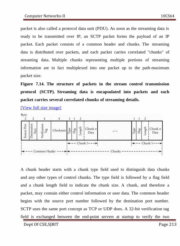
Computer Networks-II 10CS64
packet is also called a protocol data unit (PDU). As soon as the streaming data is
ready to be transmitted over IP, an SCTP packet forms the payload of an IP
packet. Each packet consists of a common header and chunks. The streaming
data is distributed over packets, and each packet carries correlated "chunks" of
streaming data. Multiple chunks representing multiple portions of streaming
information are in fact multiplexed into one packet up to the path-maximum
packet size.
Figure 7.14. The structure of packets in the stream control transmission
protocol (SCTP). Streaming data is encapsulated into packets and each
packet carries several correlated chunks of streaming details.
[View full size image]
A chunk header starts with a chunk type field used to distinguish data chunks
and any other types of control chunks. The type field is followed by a flag field
and a chunk length field to indicate the chunk size. A chunk, and therefore a
packet, may contain either control information or user data. The common header
begins with the source port number followed by the destination port number.
SCTP uses the same port concept as TCP or UDP does. A 32-bit verification tag
field is exchanged between the end-point servers at startup to verify the two
Dept Of CSE,SJBIT Page 213
Computer Networks-II 10CS64
servers involved. Thus, two tag values are used in a connection. The common
header consists of 12 bytes. SCTP packets are protected by a 32-bit checksum.
The level of protection is more robust than the 16-bit checksum of TCP and
UDP.
Each packet has n chunks, and each chunk is of two types: payload data chunk
for transmitting actual streaming data and control chunks for signaling and
control. Signaling and control chunks are of several different types, as follows:
• Initiation, to initiate an SCTP session between two end points
• Initiation acknowledgment, to acknowledge the initiation of an SCTP session
• Selective acknowledgment, to be transmitted to a peer end point to acknowledge
received data chunks
• Heartbeat request, to probe the reachability of a particular destination transport
address defined in the session
• Heartbeat acknowledgment, to respond to the heartbeat request chunk
• Abort, to close a session
• Shutdown, to initiate a graceful close of a session
• Shutdown acknowledgment, to acknowledge receipt of the shutdown chunk once
the shutdown process is completed
• Operation error, to notify the other party of a certain error
• State cookie, sent by the source to its peer to complete the initialization process
• Cookie acknowledgment, to acknowledge receipt of a state cookie chunk
• Shutdown complete, to acknowledge receipt of the shutdown acknowledgment
chunk at the completion of the shutdown process
SCTP can easily and effectively be used to broadcast live video clips or full-
Dept Of CSE,SJBIT Page 214

Computer Networks-II 10CS64
color video movies. The SCTP exercises at the end of this chapter explore SCTP
further.
Dept Of CSE,SJBIT Page 215

Computer Networks-II 10CS64
UNIT – 8
Mobile AdHoc Networks and Wireless Sensor Neworks: Overview of
Wireless Ad-Hoc networks, Routing in AdHOc Networks, Routing protocols for
and Security of AdHoc networks, Sensor Networks and protocol structures,
Communication Energy model, Clustering protocols, Routing protocols,
ZigBee technology and 802.15.4.
Dept Of CSE,SJBIT Page 216
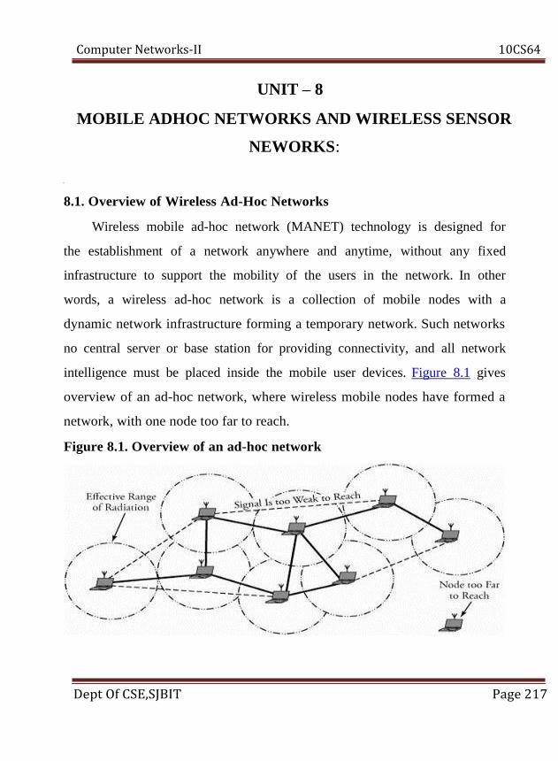
Computer Networks-II 10CS64
UNIT – 8
MOBILE ADHOC NETWORKS AND WIRELESS SENSOR
NEWORKS:
8.1. Overview of Wireless Ad-Hoc Networks
Wireless mobile ad-hoc network (MANET) technology is designed for
the establishment of a network anywhere and anytime, without any fixed
infrastructure to support the mobility of the users in the network. In other
words, a wireless ad-hoc network is a collection of mobile nodes with a
dynamic network infrastructure forming a temporary network. Such networks
no central server or base station for providing connectivity, and all network
intelligence must be placed inside the mobile user devices. Figure 8.1 gives
overview of an ad-hoc network, where wireless mobile nodes have formed a
network, with one node too far to reach.
Figure 8.1. Overview of an ad-hoc network
Dept Of CSE,SJBIT Page 217

Computer Networks-II 10CS64
In such an environment, each mobile user acts as a routing node, and a packet
is routed from a source to its destination by incorporating of other network
users. Since the topology of an ad-hoc network can change quickly and
unpredictably, it should be adaptable to changes, such as when a link breaks,
a node leaves the network, or a new node is attached to the network. Thus,
unlike intradomain routing algorithm for regular networks, if a node leaves an
ad-hoc network, all affected nodes can discover new routes. Ad-hoc networks
have several types of applications
• Rescue operations. In an emergency public disaster, such as an earthquake,
ad-hoc networks can be set up at a location where no infrastructure is present.
Ad-hoc networks can be used to support network connectivity when no fixed
network is available.
• Military. Ad-hoc networks can be used in a battle zone, for a military
command and mobile units.
• Law enforcement and security operations. An ad-hoc network can be used in
a temporary security operation, acting as a mobile surveillance network.
• Home networks. An ad-hoc network can be used to support seamless
connectivity among various devices.
• Conferencing. Ad-hoc networks can be set up for a presentation. An audience
can download a presentation, browse the slides on a portable device, print
them on the local printer, or e-mail the presentation to an absent colleague.
Ad-hoc networks must possess several unique features. One is automatic
discovery of available services. Each time a new service becomes available,
an ad hoc networking device has to configure use of the new service. As an
Dept Of CSE,SJBIT Page 218
Computer Networks-II 10CS64
ad-hoc network lacks centralized administration, the network must be able to
prevent network collapse when one of the mobile nodes moves out of
transmitter range. In general, nodes should be able to enter or leave the
network as they wish. Thus, every node acts as both a host and a router, and
the network must be intelligent enough to handle network dynamics. This
property is called self-stabilization.
One of the most common tasks of an ad-hoc network is to multicast a
message to many users efficiently. In such an environment, networks are
subject to severe blocking. Thus, the performance of an ad hoc system
depends on the stability of the network architecture. The inclusion of all these
features in ad-hoc networks requires considerable architectue sophistication.
8.2. Routing in Ad-Hoc Networks:
The lack of a backbone infrastructure makes packet routing in ad-hoc
networks a challenging task. A routing protocol should be able to automatically
recover from any problem in a finite amount of time without human intervention.
Conventional routing protocols are designed for nonmoving infrastructures and
assume that routes are bidirectional, which is not always the case for ad-hoc
networks. Identification of mobile terminals and correct routing of packets to and
from each terminal while moving are certainly challenging.
Since the topology of an ad-hoc network is dynamic, reserving resources and
sustaining QoS are difficult. In an ad-hoc medium, it may not be possible to
communicate bidirectionally, so ad-hoc routing protocols should assume that
Dept Of CSE,SJBIT Page 219
Computer Networks-II 10CS64
links are unidirectional. The power of a wireless device is another important
factor. The routing protocol also has to support node stand-by mode. Devices
such as laptops are very limited in battery power; hence, the use of stand-by
mode to save power is important.
8.2.1. Classification of Routing Protocols
Ad-hoc routing protocols can be classified into two broad categories:
1. Centralized versus distributed. In centralized routing protocols, the routing
decision is made at a central node. In distributed routing protocols, the routing
decision is made by all the network nodes. Routing protocols in most efficiently
designed ad-hoc networks are distributed to increase the reliability of the
network. In such cases, nodes can enter or leave the network easily, and each
node can make routing decisions, using other collaborative nodes.
2. Static versus adaptive. In static routing protocols, a route of a source/destination
pair does not change because of any traffic condition or link failure. In adaptive
routing protocols, routes may change because of any congestion.
Whether a protocol is centralized, distributed, static, or adaptive, it can generally
be categorized as either table driven or source initiated.
Table-Driven Routing Protocols
Table-driven, or proactive, routing protocols find routes to all possible
destinations ahead of time. are needed. The routes are recorded in the nodes'
routing tables and are updated within the predefined intervals. Proactive
protocols are faster in decision making but need more time to converge to a
steady state, causing problems if the topology of the network continually
changes. However, maintaining routes can lead to a large overhead. Table-driven
Dept Of CSE,SJBIT Page 220
Computer Networks-II 10CS64
protocols require every node to maintain one or more tables to store updated
routing information from every node to all other nodes. Nodes propagate updated
tables all over the network such that the routing information in each table
corresponds to topological changes in the network.
Source-Initiated Routing Protocols
Source-initiated, or reactive, routing protocols, are on-demand procedures and
create routes only when requested to do so by source nodes. A route request
initiates a route-discovery process in the network and is completed once a route
is discovered. If it exists at the time of a request, a route is maintained by a route-
maintenance procedure until either the destination node becomes irrelevant to the
source or the route is no longer needed. On-demand protocols are more suitable
for ad-hoc networks. In most cases, reactive protocols are desired. This means
that the network reacts only when needed and does not broadcast information
periodically. However, the control overhead of packets is smaller than for
proactive protocols.
Routing Protocols for Ad-Hoc Networks
This section discusses three table-driven protocols and four source-initiated
protocols. The table-driven protocols are the Destination-Sequenced Distance
Vector (DSDV) protocol, the Cluster-Head Gateway Switch Routing (CGSR)
protocol, and the Wireless Routing Protocol (WRP). The source-initiated
protocols are the Dynamic Source Routing (DSR) protocol, the Associative-
Based Routing (ABR) protocol, Temporally Ordered Routing Algorithm
(TORA), and Ad-Hoc On-Demand Distance Vector (AODV) protocol.
8.2.1. Destination-Sequenced Distance Vector (DSDV) Protocol
Dept Of CSE,SJBIT Page 221
Computer Networks-II 10CS64
The Destination-Sequenced Distance Vector (DSDV) protocol is a table-driven
routing protocol based on the improved version of classical Bellman-Ford
routing algorithm. DSDV is based on the Routing Information Protocol (RIP),
explained in Chapter 7. With RIP, a node holds a routing table containing all the
possible destinations within the network and the number of hops to each
destination. DSDV is also based on distance vector routing and thus uses
bidirectional links. A limitation of DSDV is that it provides only one route for a
source/destination pair.
Routing Tables
The structure of the routing table for this protocol is simple. Each table entry has
a sequence number that is incremented every time a node sends an updated
message. Routing tables are periodically updated when the topology of the
network changes and are propagated throughout the network to keep consistent
information throughout the network.
Each DSDV node maintains two routing tables: one for forwarding packets and
one for advertising incremental routing packets. The routing information sent
periodically by a node contains a new sequence number, the destination address,
the number of hops to the destination node, and the sequence number of the
destination. When the topology of a network changes, a detecting node sends an
update packet to its neighboring nodes. On receipt of an update packet from a
neighboring node, a node extracts the information from the packet and updates
its routing table as follows
Dept Of CSE,SJBIT Page 222
Computer Networks-II 10CS64
DSDV Packet Process Algorithm
1. If the new address has a higher sequence number, the node chooses the route
with the higher sequence number and discards the old sequence number.
2. If the incoming sequence number is identical to the one belonging to the existing
route, a route with the least cost is chosen.
3. All the metrics chosen from the new routing information are incremented.
4. This process continues until all the nodes are updated. If there are duplicate
updated packets, the node considers keeping the one with the least-cost metric
and discards the rest.
In case of a broken link, a cost of metric with a new sequence number
(incremented) is assigned to it to ensure that the sequence number of that metric
is always greater than or equal to the sequence number of that node. Figure 8.2
shows a routing table for node 2, whose neighbors are nodes 1, 3, 4, and 8. The
dashed lines indicate no communications between any corresponding pair of
nodes. Therefore, node 2 has no information about node 8.
Dept Of CSE,SJBIT Page 223

Computer Networks-II 10CS64
Figure 8.2. A DSDV routing table
The packet overhead of the DSDV protocol increases the total number of nodes
in the ad-hoc network. This fact makes DSDV suitable for small networks. In
large adhoc networks, the mobility rateand therefore the overheadincrease,
making the network unstable to the point that updated packets might not reach
nodes on time.
8.2.2. Cluster-Head Gateway Switch Routing Protocol
The Cluster-Head Gateway Switch Routing (CGSR) protocol is a table-driven
routing protocol. In a clustering system. each predefined number of nodes are
formed into a cluster controlled by a cluster head, which is assigned using a
distributed clustering algorithm. However, with the clustering scheme, a cluster
Dept Of CSE,SJBIT Page 224

Computer Networks-II 10CS64
head can be replaced frequently by another node, for several reasons, such as
lower-level energy left in the node or a node moves out of contact.
With this protocol, each node maintains two tables: a cluster-member table and a
routing table. The cluster-member table records the cluster head for each
destination node, and the routing table contains the next hop to reach the
destination. As with the DSDV protocol, each node updates its cluster-member
table on receiving a new update from its neighbors.
Clustering and Routing Algorithms
CGSR routing involves cluster routing, whereby a node is required to find the
best route over cluster heads from the cluster-member table. Figure 19.3 shows
an example of routing in an area in which six clusters have been formed. A node
in cluster A is transmitting a packet to a node in cluster F. Nodes within each
cluster route their packets to their own associated clusters. The transmitting node
then sends its packet to the next hop, according to the routing table entry
associated with that cluster head. The cluster head transmits the packet to another
cluster head until the cluster head of the destination node is reached. The routing
is made through a series of available cluster heads from A to F. Packets are then
transmitted to the destination.
Figure 8.2. Communication with cluster-head gateway switch routing
(CGSR) protocol
Dept Of CSE,SJBIT Page 225

Computer Networks-II 10CS64
8.2.3. Wireless Routing Protocol (WRP)
The Wireless Routing Protocol (WRP) is a table-based protocol maintaining
routing information among all nodes in the network. This protocol is based on
the distributed Bellman-Ford algorithm. The main advantage of WRP is that it
reduces the number of routing loops. With this protocol, each node in a network
maintains four tables, as follows:
1. Distance table, which holds the destination, next hop, distance, and predecessors
of each destination and each neighbor.
2. Routing table, which saves the destination address, next hop, distance,
predecessor, and a marker for each destination, specifying whether that entry
corresponds to a simple path.
Dept Of CSE,SJBIT Page 226

Computer Networks-II 10CS64
3. Link-cost table, which provides the link cost to each neighbor and also the
number of periodic update periods elapsed since the node received any error-free
message from it.
4. Message transmission-list table, which records which updates in an update
message are to be retransmitted and which neighbors need to acknowledge the
retransmission. The table provides the sequence number of the update message, a
retransmission counter, acknowledgments, and a list of updates sent in the update
message.
Nodes should either send a message including the update message or a HELLO
message to their neighbors. If a node has no message to send, it should send a
HELLO message to ensure connectivity. If the sending node is new, it is added
to the node's routing table, and the current node sends the new node a copy of its
routing table content.
Once it detects a change in a route, a node sends the update message to its
neighbors. The neighboring nodes then change their distance entries and look for
new possible paths through other nodes. This protocol avoids the count-to-
infinity issue present in most ad-hoc network protocols. This issue is resolved by
making each node perform consistency checks of predecessor information
reported by all its neighbors in order to remove looping and make a faster route
convergence in the presence of any link or node failure.
Dept Of CSE,SJBIT Page 227

Computer Networks-II 10CS64
8.3 Routing protocols for and Security of AdHoc networks:
This section discusses three table-driven protocols and four source-initiated
protocols. The table-driven protocols are the Destination-Sequenced Distance
Vector (DSDV) protocol, the Cluster-Head Gateway Switch Routing (CGSR)
protocol, and the Wireless Routing Protocol (WRP). The source-initiated
protocols are the Dynamic Source Routing (DSR) protocol, the Associative-
Based Routing (ABR) protocol, Temporally Ordered Routing Algorithm
(TORA), and Ad-Hoc On-Demand Distance Vector (AODV) protocol.
8.3.1. Destination-Sequenced Distance Vector (DSDV) Protocol
The Destination-Sequenced Distance Vector (DSDV) protocol is a table-driven
routing protocol based on the improved version of classical Bellman-Ford
routing algorithm. DSDV is based on the Routing Information Protocol (RIP),
explained in Chapter 7. With RIP, a node holds a routing table containing all the
possible destinations within the network and the number of hops to each
destination. DSDV is also based on distance vector routing and thus uses
bidirectional links. A limitation of DSDV is that it provides only one route for a
source/destination pair.
Routing Tables
The structure of the routing table for this protocol is simple. Each table entry has
a sequence number that is incremented every time a node sends an updated
message. Routing tables are periodically updated when the topology of the
network changes and are propagated throughout the network to keep consistent
information throughout the network.
Dept Of CSE,SJBIT Page 228
Computer Networks-II 10CS64
Each DSDV node maintains two routing tables: one for forwarding packets and
one for advertising incremental routing packets. The routing information sent
periodically by a node contains a new sequence number, the destination address,
the number of hops to the destination node, and the sequence number of the
destination. When the topology of a network changes, a detecting node sends an
update packet to its neighboring nodes. On receipt of an update packet from a
neighboring node, a node extracts the information from the packet and updates
its routing table as follows
DSDV Packet Process Algorithm
5. If the new address has a higher sequence number, the node chooses the route
with the higher sequence number and discards the old sequence number.
6. If the incoming sequence number is identical to the one belonging to the existing
route, a route with the least cost is chosen.
7. All the metrics chosen from the new routing information are incremented.
8. This process continues until all the nodes are updated. If there are duplicate
updated packets, the node considers keeping the one with the least-cost metric
and discards the rest.
In case of a broken link, a cost of metric with a new sequence number
(incremented) is assigned to it to ensure that the sequence number of that metric
is always greater than or equal to the sequence number of that node. Figure 8.2
shows a routing table for node 2, whose neighbors are nodes 1, 3, 4, and 8. The
dashed lines indicate no communications between any corresponding pair of
nodes. Therefore, node 2 has no information about node 8.
Dept Of CSE,SJBIT Page 229
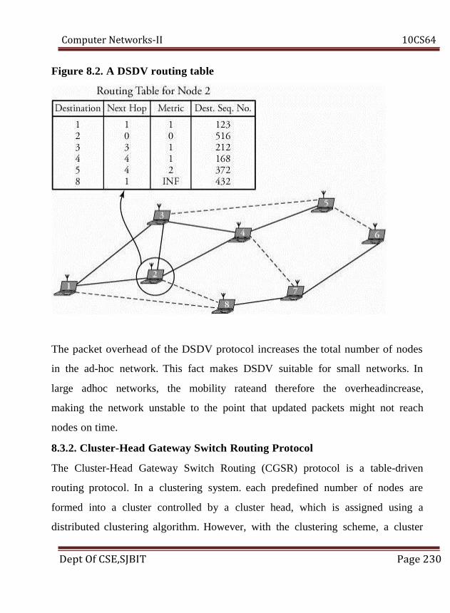
Computer Networks-II 10CS64
Figure 8.2. A DSDV routing table
The packet overhead of the DSDV protocol increases the total number of nodes
in the ad-hoc network. This fact makes DSDV suitable for small networks. In
large adhoc networks, the mobility rateand therefore the overheadincrease,
making the network unstable to the point that updated packets might not reach
nodes on time.
8.3.2. Cluster-Head Gateway Switch Routing Protocol
The Cluster-Head Gateway Switch Routing (CGSR) protocol is a table-driven
routing protocol. In a clustering system. each predefined number of nodes are
formed into a cluster controlled by a cluster head, which is assigned using a
distributed clustering algorithm. However, with the clustering scheme, a cluster
Dept Of CSE,SJBIT Page 230
Computer Networks-II 10CS64
head can be replaced frequently by another node, for several reasons, such as
lower-level energy left in the node or a node moves out of contact.
With this protocol, each node maintains two tables: a cluster-member table and a
routing table. The cluster-member table records the cluster head for each
destination node, and the routing table contains the next hop to reach the
destination. As with the DSDV protocol, each node updates its cluster-member
table on receiving a new update from its neighbors.
Clustering and Routing Algorithms
CGSR routing involves cluster routing, whereby a node is required to find the
best route over cluster heads from the cluster-member table. Figure 8.3 shows an
example of routing in an area in which six clusters have been formed. A node in
cluster A is transmitting a packet to a node in cluster F. Nodes within each
cluster route their packets to their own associated clusters. The transmitting node
then sends its packet to the next hop, according to the routing table entry
associated with that cluster head. The cluster head transmits the packet to another
cluster head until the cluster head of the destination node is reached. The routing
is made through a series of available cluster heads from A to F. Packets are then
transmitted to the destination.
Dept Of CSE,SJBIT Page 231
Computer Networks-II 10CS64
Figure 8.3. Communication with cluster-head gateway switch routing
(CGSR) protocol
8.3.3. Wireless Routing Protocol (WRP)
The Wireless Routing Protocol (WRP) is a table-based protocol maintaining
routing information among all nodes in the network. This protocol is based on
the distributed Bellman-Ford algorithm. The main advantage of WRP is that it
reduces the number of routing loops. With this protocol, each node in a network
maintains four tables, as follows:
5. Distance table, which holds the destination, next hop, distance, and predecessors
of each destination and each neighbor.
Dept Of CSE,SJBIT Page 232
Computer Networks-II 10CS64
6. Routing table, which saves the destination address, next hop, distance,
predecessor, and a marker for each destination, specifying whether that entry
corresponds to a simple path.
7. Link-cost table, which provides the link cost to each neighbor and also the
number of periodic update periods elapsed since the node received any error-free
message from it.
8. Message transmission-list table, which records which updates in an update
message are to be retransmitted and which neighbors need to acknowledge the
retransmission. The table provides the sequence number of the update message, a
retransmission counter, acknowledgments, and a list of updates sent in the update
message.
Nodes should either send a message including the update message or a HELLO
message to their neighbors. If a node has no message to send, it should send a
HELLO message to ensure connectivity. If the sending node is new, it is added
to the node's routing table, and the current node sends the new node a copy of its
routing table content.
Once it detects a change in a route, a node sends the update message to its
neighbors. The neighboring nodes then change their distance entries and look for
new possible paths through other nodes. This protocol avoids the count-to-
infinity issue present in most ad-hoc network protocols. This issue is resolved by
making each node perform consistency checks of predecessor information
reported by all its neighbors in order to remove looping and make a faster route
convergence in the presence of any link or node failure.
8.3.4. Dynamic Source Routing (DSR) Protocol
Dept Of CSE,SJBIT Page 233

Computer Networks-II 10CS64
The Dynamic Source Routing (DSR) protocol is an on-demand, or source-
initiated, routing protocol in which a source node finds an unexpired route to a
destination to send the packet. DSR quickly adapts to topological changes and is
typically used for networks in which mobile nodes move with moderate speed.
Overhead is significantly reduced with this protocol, since nodes do not
exchange routing table information when there are no changes in the topology.
DSR creates multiple paths from a source to a destination, eliminating route
discovery when the topology changes. Similar to most ad-hoc networks, DSR
has two phases: route discovery and route maintenance.
Route Discovery and Maintenance
Route discovery is initiated when a node wants to send packets to another node
and no unexpired route to the destination is in its routing table. In such
circumstances, the node first broadcasts a route-request packet, including the
destination address, source address, and a unique identification number. When it
receives a route-request packet, the neighboring node it looks at its table; if any
route to the requested destination address is already present in the node's route
record, the packet is discarded to avoid the looping issue. Otherwise, the node
adds its own address to the preassigned field of the route-request packet and
forwards it to its neighboring nodes.
When the route-request packet reaches a destination node or another
intermediate node that has an unexpired route to the destination, this node
generates a route-reply packet, which contains a route record of the sequence of
nodes taken from the source to this node. Once the source receives all the route-
reply packets, it updates its routing table with the best path to the destination and
Dept Of CSE,SJBIT Page 234
Computer Networks-II 10CS64
sends its packets through that selected route.
8.4 Sensor Networks and protocol structures:
Chemical, biological, or solar sensors can be networked together as a sensor
network to strengthen the power of sensing. A sensor network is controlled
through a software core engine. The network is typically wireless but may also
be wired. Sensor networks are designed to be self-configuring such that they can
gather information about a large geographical area or about movements of an
object for surveillance purposes.
Sensor networks can be used for target tracking, environmental monitoring,
system control, and chemical or biological detection. In military applications,
sensor networks can enable soldiers to see around corners and to detect chemical
and biological weapons long before they get close enough to cause harm.
Civilian uses include environmental monitoring, traffic control, and providing
health care monitoring for the elderly while allowing them more freedom to
move about.
8.4.1. Clustering in Sensor Networks
The region being sensed is normally partitioned into equally loaded clusters
of sensor nodes, as shown in Figure 8.1. A cluster in a sensor network resembles
a domain in a computer network. In other words, nodes are inserted in the
vicinity of a certain predefined region, forming a cluster. Different types of
sensors can also be deployed in a region. Thus, a sensor network is typically
cluster based and has irregular topology. The most effective routing scheme in
sensor networks is normally based on the energy (battery level) of nodes. In such
Dept Of CSE,SJBIT Page 235

Computer Networks-II 10CS64
routing schemes, the best path has the highest amount of total energy. The
network of such sensing nodes is constructed with identical sensor nodes,
regardless of the size of the network. In Figure 8.1, three clusters are
interconnected to the main base station, each cluster contains a cluster head
responsible for routing data from its corresponding cluster to a base station.
Figure 8.1. A sensor network and its clusters
Communicating nodes are normally linked by a wireless medium, such as radio.
The wireless sensor node is equipped with a limited power source, such as a
battery or even a solar cell, where there is enough sunlight exposure on the node.
However, a solar cell may not be the best choice as a power supply, owing to its
weight, volume, and expense. In some application scenarios, sensor-node
lifetime depends on the battery lifetime. Removal of dead nodes can cause
significant topological changes and may require packet rerouting. As a result,
power management is a key issue in system design, node design, and
Dept Of CSE,SJBIT Page 236
Computer Networks-II 10CS64
communication protocol development. In summary, efficient energy-conscious
clustering and routing algorithms can potentially prolong the network lifetime.
8.4.2. Protocol Stack
The algorithms developed for wireless ad-hoc networks cannot be used for
sensor networks, for several reasons. One is that the number of sensor nodes is
typically much more than in a typical ad-hoc network, and sensor nodes, unlike
ad-hoc nodes, are prone to permanent failure. In addition, sensor nodes normally
use broadcast rather than point-to-point communication with its limited power
and memory. Unlike computer networks, sensor nodes do not have global ID,
since a typical packet overhead can be too large for them.
Figure 8.2 shows protocol architecture for sensor networks. The protocol stack
combines power efficiency and least-cost-path routing. This protocol architecture
integrates networking protocols and power through the wireless medium and
promotes cooperative efforts of sensor nodes. The protocol stack consists of the
physical layer, data-link layer, network layer, transport layer, and application
layer, backed by a power-management plane, mobility-management plane, and
task-management plane. The physical layer is responsible for robust modulation,
transmission, and receiving signals. Media access control (MAC) at the data-link
layer must minimize packet collision with neighboring nodes, as power is a
restricted factor. The network layer routes packets provided by the transport
layer. The application layer uses software for preparation of data on an event.
The power-management plane monitors the sensor's power level among the
sensor nodes and manages the amount of power a sensor node has used.
Dept Of CSE,SJBIT Page 237

Computer Networks-II 10CS64
Figure 8.2. Sensor network protocol stack architecture
Most of the sensor network routing techniques and sensing tasks require an
accurate knowledge of location. Thus, a sensor node commonly has a location-
finding system. A mobilizer may sometimes be needed to move sensor nodes to
carry out assigned tasks. Sensor network routing protocols must be capable of
self-organizing. For these purposes, a series of energy-aware MAC, routing, and
clustering protocols have been developed for wireless sensor networks. Most of
the energy-aware MAC protocols aim to either adjust the transmission power or
keep transceivers off as long as possible.
8.4.3. Sensor Node Structure
Figure 8.3 shows a typical sensor node. A node consists mainly of a sensing unit,
a processing unit and memory, a self-power unit, and a wireless transceiver
Dept Of CSE,SJBIT Page 238

Computer Networks-II 10CS64
component, as well as a self- and remote-testing unit, a synchronizing and timing
unit, a routing table, and security units. Since nodes in a network are not
physically accessible once they are deployed in the field, they are not worth
being brought under test. An option is an on-board remote self-testing unit for
the node on a routine basis.
Figure 8.3. A typical wireless sensor node
Each node must determine its location. This task is carried out by a location-
finding system based on the global positioning system (GPS). All the processes
within the sensor node are synchronized by a local clocking and synchronizing
system. The communication and security protocol units are in fact part of the
processing unit. These two units are responsible for computing the best path for
networking and security of the data being transmitted. The three main blocks of
the sensor nodesensing unit, processing and memory unit, and power unitare
described in more detail in the following subsections.
Dept Of CSE,SJBIT Page 239
Computer Networks-II 10CS64
Sensing Unit
The sensing unit consists of a sensor and an analog-to-digital converter. A smart
sensor node consists of a combination of multiple sensors. The analog signals
produced by the sensors, based on the observed event, are converted to digital
signals by the converter and then fed into the processing unit. The sensing unit
collects data externally and interacts with the central processor at the heart of the
node.
Processing and Memory Unit
The processing unit performs certain computations on the data and,
depending on how it is programmed, may send the resulting information out to
the network. The processing unit, which is generally associated with memory,
manages the procedures that make the sensor node collaborate with the other
nodes to carry out the assigned sensing task. The central processor determines
what data needs to be analyzed, stored, or compared with the data stored in
memory. The streamed data from the sensor input is processed as it arrives. The
database in memory stores an indexed data list to be used as a reference to detect
an event. Since sensing nodes are typically tiny and many nodes are engaged in a
network, the communication structure makes use of a hierarchically arranged
self-routing network through cluster heads.
In smart wireless sensor networks, a tiny processor and a tiny database are
used in a node. Thousands of such nodes are spread on fields to power up the
sensing task, as in the deployment of numerous small intelligent sensor nodes in
a battlefield to monitor enemy movements. By inserting self-organizing
capability into a sensor network, a smart node can extract data, compare it with
Dept Of CSE,SJBIT Page 240

Computer Networks-II 10CS64
the data stored in its memory database, and process it for relevance before
relaying it to its central base station.
Self-Power Unit
A sensor node is supposed to be mounted in a small physical unit,
limiting space for the battery. Moreover, the random distribution of sensors
makes it impossible to periodically recharge or exchange batteries. In most types
of sensor networks, the power unit in a sensor node is the most important unit of
the node because the liveliness and existence of a node depend on the energy left
in the node, and the routing in the sensor network is based on the algorithm that
finds a path with the most energy. Thus, it is essential to use energy-efficient
algorithms to prolong the life of sensor networks. The main task of the sensor
node is to identify events, to process data, and then to transmit the data. The
power of a node is consumed mainly in the transmitter and receiver unit. The
sensor node can be supplied by a self-power unit, self-power unitbattery, or solar
cells.
8.5 Communication Energy model:
IEEE standardsas 802.11a, b, and g provide a wide range of data rates:
54, 48, 36, 24, 18, 12, 9, and 6 Mb/s. This range reflects the trade-off between
the transmission range and data rate intrinsic in a wireless communication
channel. An accurate energy model is crucial for the development of energy-
efficient clustering and routing protocols. The energy consumption, E, for all
components of the transceiver in watts is summarized as
Dept Of CSE,SJBIT Page 241

Computer Networks-II 10CS64
Equation 8.1
where θ is the distance-independent term that accounts for the overhead of the
radio electronics and digital processing, and ηωdn, is the distance-dependent
term, in which η represents the amplifier inefficiency factor, ω is the free-space
path loss, d is the distance, and n is the environmental factor. Based on an
environmental condition, n can be a number between 2 and 4, and η specifies the
inefficiency of the transmitter when generating maximum power ωdn at the
antenna. Clearly, the distance-dependent portion of total energy consumption
depends on the real-world transceiver parameters, θ, η, and the path attenuation
ωdn. If the value of θ overshadows ηωdn, the reduction in the transmission
distance through the use of multihop communication is not effective.
In theory, the maximum efficiency of a power amplifier is 48.4 percent.
However, practical implementations show that the power-amplifier efficiency is
less than 40 percent. Therefore, θ is calculated assuming that η = 1/0.4 = 2.5.
Using Equation (8.1), we can express the energy consumption of a transmitter
and a receiver, ET and ER, respectively, by
Equation 20.2
and
Equation 20.3
Dept Of CSE,SJBIT Page 242

Computer Networks-II 10CS64
where θT and θR are the distance-dependent terms for the transmitter and the
receiver, respectively. Although maximum output power and total power
consumption are provided in the manufacturer's data sheet, θ can be calculated
the following formula:
Equation 20.4
8.6 Clustering protocols:
Clustering protocols specify the topology of the hierarchical
nonoverlapping clusters of sensor nodes. A robust clustering technique is
essential for self-organizing sensor networks. An efficient clustering protocol
ensures the creation of clusters with almost the same radius and cluster heads
that are best positioned in the clusters. Since every node in a clustered network is
connected to a cluster head, route discovery among cluster heads is sufficient to
establish a feasible route in the network. For a large sensor network, clustering
can simplify multihop route discovery and limit the number of transmissions
compared to a flat, nonclustered network.
8.6.1. Classification of Clustering Protocols
Clustering techniques can be either centralized or decentralized. Centralized
clustering algorithms require each sensor node to send its individual information,
such as energy level and geographical position, to the central base station. Based
on a predefined algorithm, a base station calculates the number of clusters, their
sizes, and the cluster heads' positions and then provides each node with its newly
Dept Of CSE,SJBIT Page 243

Computer Networks-II 10CS64
assigned duty.
Given the assumption that sensor networks might consist of thousands of
nodes, it is impractical, if not impossible, for a base station to collect information
about every node in the network prior to route setup. Therefore, centralized
clustering is not an option for large sensor networks. Since a sensor node begins
a clustering process without any knowledge about its location relative to the
corresponding base station, a clustering algorithm should be able to form clusters
without the help of the base station and knowledge of node positioning.
Although location-finder devices can also be deployed to perform this task, they
are often either costly or add too much overhead on the network.
Decentralized clustering techniques create clusters without the help of any
centralized base station. An energy-efficient and hierarchical clustering
algorithm can be such a way whereby each sensor node becomes a cluster head
with a probability of p and advertises its candidacy to nodes that are no more
than k hops away from the cluster head. Given the limited transmission range of
wireless sensor nodes, a hierarchical structure with an arbitrary number of levels
has its limitations. As the number of hierarchical levels grows, the distance
between upper-level cluster heads may increase to the point that they are no
longer able to communicate with one another. The Low-Energy Adaptive
Clustering Hierarchy (LEACH) algorithm and the Decentralized Energy-
Efficient Cluster Propagation (DEEP) protocol are two examples of the
decentralized clustering protocols and are explained next.
Dept Of CSE,SJBIT Page 244
Computer Networks-II 10CS64
8.6.2. LEACH Clustering Protocol
The Low-Energy Adaptive Clustering Hierarchy (LEACH) protocol is a
decentralized clustering algorithm that does not offer a complete energy-
optimization solution, as it has no strategy for specifying cluster-head
positioning and distribution. LEACH is an application-specific protocol
architecture that aims to prolong network lifetime by periodic reclustering and
change of the network topology.
LEACH is divided into rounds consisting of a clustering phase and a
steady-state phase for data collection. At the start of each round, a sensor node
randomly chooses a number between 0 and 1 and then compares this number to a
calculated threshold called T(n). If T(n) is larger than the chosen number, the
node becomes a cluster head for the current round. The value T(n) is calculated
using the following formula:
Equation 20.11
where p is the ratio of the total number of cluster heads to the total number of
nodes, r is the number of rounds, and G is a set of nodes that have not been
chosen as cluster heads for the last 1/p rounds. For the first round (r=0), T(n) is
equal to p, and nodes have an equal chance to become cluster head. As r gets
closer to 1/p, T(n) increases, and nodes that have not been selected as cluster
head in the last 1/p rounds have more chance to become cluster head. After 1/p -
1 rounds, T(n) is equal to 1, meaning that all the remaining nodes have been
Dept Of CSE,SJBIT Page 245

Computer Networks-II 10CS64
selected as cluster head. Thus, after 1/p rounds, all the nodes have had a chance
to become a cluster head once. Since being the cluster head puts a substantial
burden on the sensor nodes, this ensures that the network has no overloaded node
that runs out of energy sooner than the others.
After cluster heads are self-selected, they start to advertise their
candidacy to the other sensor nodes. When it receives advertisements from more
than one cluster-head candidate, a sensor node starts to make a decision about its
corresponding cluster head. Each node listens to the advertisement signals and
chooses the candidate whose associated signal is received with higher power.
This ensures that each sensor node chooses the closest candidate as cluster head.
The LEACH algorithm is distributed, as it can be accomplished by local
computation and communication at each node, rather than the transmission of all
the nodes' energy level and geographical position to a centralized point.
However, cluster heads are chosen randomly, and there is no optimization in
terms of energy consumption.
8.7 Routing protocols:
After clusters with well-distributed cluster heads have been established in
a network, energy-conscious routing is essential in order to set communication
routes among cluster heads in a two-level hierarchical system. Similar to
computer networks, routing protocols in sensor networks can be classified as
either intracluster or intercluster. This section looks at both categories.
The fundamental concept behind them is much the same as the concept behind
intradomain and interdomain routings Assuming that every node in a cluster can
Dept Of CSE,SJBIT Page 246
Computer Networks-II 10CS64
act as a relay node, there could be a large number of possible routes from a
source to a sink. Because of the limited transmission range associated with low-
power wireless technologies cluster-head packets cannot reach the base station
unless other cluster heads act as relay nodes. Two major approaches can be used
for routing and selecting the best path in a sensor network, as follows:
1. Centralized routing, whereby the routing decision is made by a single command
center
2. Distributed routing, whereby the routing decision is made in a distributed fashion
by several entities
Distributed routing algorithms are further classified as proactive or reactive.
With proactive routing algorithms, such as link-state routing and distance-vector
routing, nodes keep a routing table that contains next-hop information to every
node in the network. Reactive routing protocols set a route to the desirable
destination only when it is needed. Note that none of the ad hoc network
protocols explained earlier considers energy consumption.
Another group of on-demand reactive routing protocols address the exclusive
issues of wireless sensor network. For example, directed diffusion introduces a
concept of "interest" propagation whenever a node wants to send data or a source
needs to ask for it. With this type of protocol, flooding the network with interest
signals establishes a path from a sink to every possible source (spanning tree).
8.7.1. Intracluster Routing Protocols
A routing algorithm within a cluster can be either direct or multihop. In a direct
routing algorithm, the cluster head as the destination for all cluster nodes is
located in the center of the cluster, so all nodes can communicate with the cluster
Dept Of CSE,SJBIT Page 247
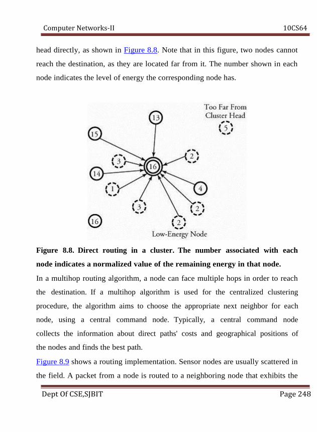
Computer Networks-II 10CS64
head directly, as shown in Figure 8.8. Note that in this figure, two nodes cannot
reach the destination, as they are located far from it. The number shown in each
node indicates the level of energy the corresponding node has.
Figure 8.8. Direct routing in a cluster. The number associated with each
node indicates a normalized value of the remaining energy in that node.
In a multihop routing algorithm, a node can face multiple hops in order to reach
the destination. If a multihop algorithm is used for the centralized clustering
procedure, the algorithm aims to choose the appropriate next neighbor for each
node, using a central command node. Typically, a central command node
collects the information about direct paths' costs and geographical positions of
the nodes and finds the best path.
Figure 8.9 shows a routing implementation. Sensor nodes are usually scattered in
the field. A packet from a node is routed to a neighboring node that exhibits the
Dept Of CSE,SJBIT Page 248

Computer Networks-II 10CS64
highest amount of energy. The energy is an indication of the node's battery level.
The number associated with each node indicates a normalized value of the
remaining energy in that node. Figure 8.9 shows two paths from a node to a
cluster-head node. One path involves the shortest distance in terms of hop
counts; the other one uses the highest-energy route. The challenge here is to find
the best path that suits the rapid and secure deployment of data. Data is routed to
the cluster head as shown in Figure 8.1, where the cluster head may
communicate with the base station via radio frequencies.
Dept Of CSE,SJBIT Page 249
Computer Networks-II 10CS64
8.8 ZigBee technology and 802.15.4:
The ZigBee technology is a communication standard that provides a
short-range low-cost networking capability that allows low-cost devices to
quickly transmit small amounts of data, such as temperature readings for
thermostats, on/off requests for light switches, or keystrokes for a wireless
keyboard. Other ZigBee applications are in professional installation kits for
lighting controls, heating, ventilation, air conditioning, and security. Even the
Bluetooth short-range wireless technology found in laptops and cellphones lacks
the affordability, power savings, and mesh-networking capabilities of ZigBee.
ZigBee comes from higher-layer enhancements by a multivendor
consortium called the Zigbee Alliance. IEEE standard 802.15.4/ZigBee specifies
the MAC and physical layers. The 802.15.4 standard specifies 128-bit AES
encryption; ZigBee specifies how to handle encryption key exchange. The
802.15.4/ZigBee networks run in the unlicensed frequencies, 900 MHz and 2.4
GHz band, based on a packet radio standard and support many cordless
telephones, allowing data to be sent over distances up to 20 meters.
ZigBee devices, typically battery powered, can transmit information
much farther than 20 meters, because each device within listening distance
passes the message along to any other device within range. Only the intended
device acts on the message. By instructing nodes to wake up only for those split-
second intervals when they are needed, ZigBee device batteries might last for
years. Although this technology is targeting for manufacturing, health care,
shipping, and homeland defense, the ZigBee Alliance is initially keeping its
focus small.
Dept Of CSE,SJBIT Page 250

Computer Networks-II 10CS64
Dept Of CSE,SJBIT Page 251


![Computer Networks-II [10CS64] Notes - VTU Solutionvtusolution.in/uploads/9/9/9/...computer_networks-ii_[10cs64]-notes... · vtusolution.in Computer Networks-II 10CS64. Security of](https://static.fdocuments.in/doc/165x107/5b36d10e7f8b9abd438b6ec7/computer-networks-ii-10cs64-notes-vtu-10cs64-notes-vtusolutionin-computer.jpg)


