Computer Graphics - Max Planck Societyresources.mpi-inf.mpg.de/departments/d4/teaching/... ·...
72
Computer Graphics WS07/08 –Tone Mapping Computer Graphics - HDR & Tone Mapping - Hendrik Lensch
Transcript of Computer Graphics - Max Planck Societyresources.mpi-inf.mpg.de/departments/d4/teaching/... ·...

Computer Graphics WS07/08 –Tone Mapping
Computer Graphics
- HDR & Tone Mapping -
Hendrik Lensch

Computer Graphics WS07/08 –Tone Mapping
Overview• Last time
– Gamma Correction– Color spaces
• Today– Terms and Definitions– Tone Mapping
• Next lecture– Transformations
Computer Graphics WS07/08 –Tone Mapping
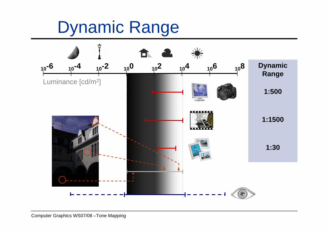
Dynamic Range
Luminance [cd/m2]
10-6 10-4 10-2 100 102 104 106 108 DynamicRange
1:500
1:1500
1:30
Computer Graphics WS07/08 –Tone Mapping
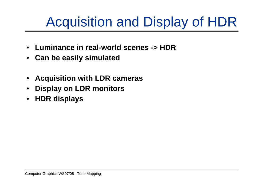
Acquisition and Display of HDR
• Luminance in real-world scenes -> HDR• Can be easily simulated
• Acquisition with LDR cameras• Display on LDR monitors• HDR displays
Computer Graphics WS07/08 –Tone Mapping
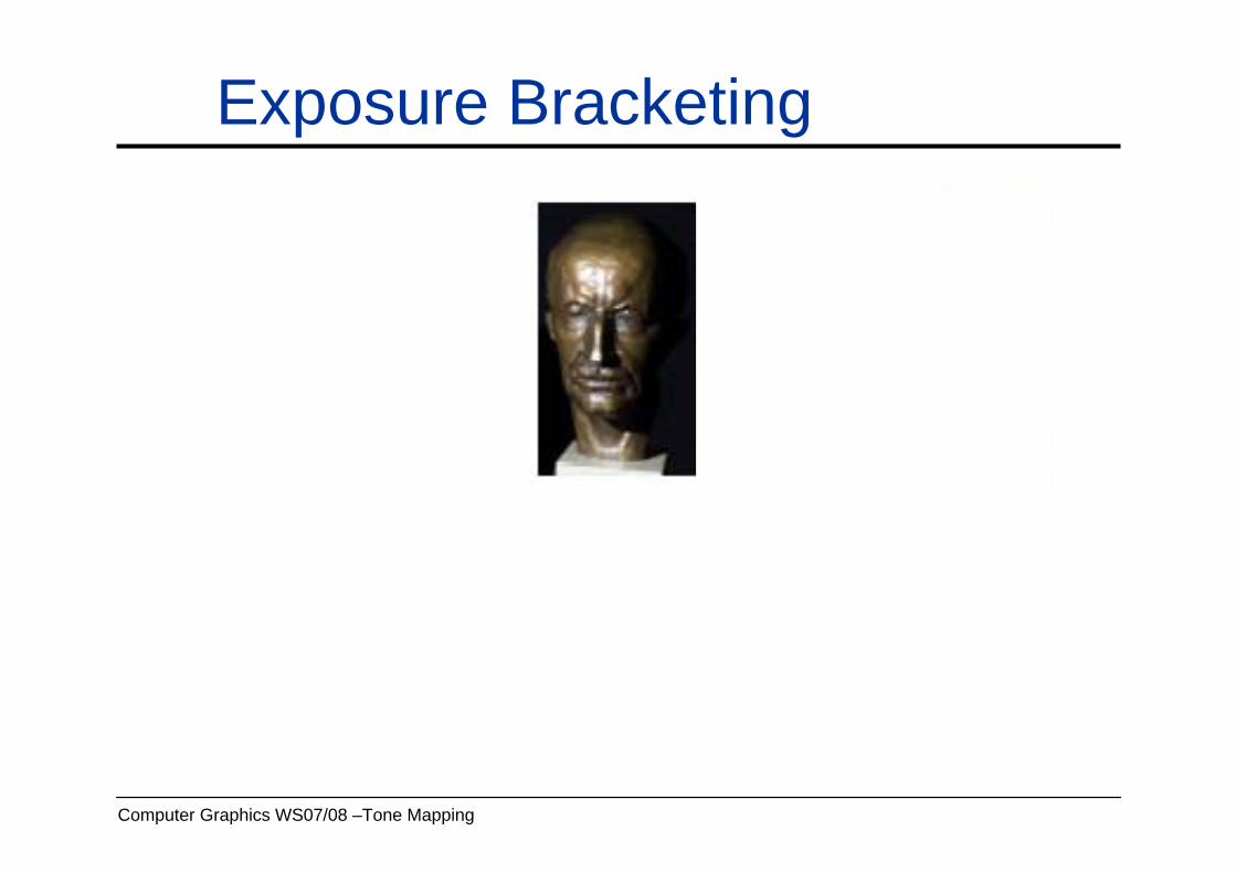
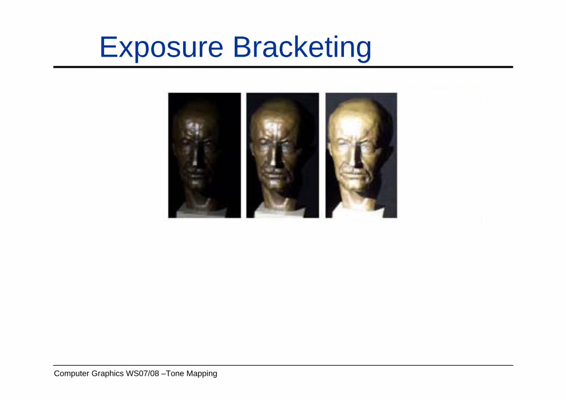
Exposure Bracketing
– capture additional over and underexposed images
Computer Graphics WS07/08 –Tone Mapping
Exposure Bracketing
– capture additional over and underexposed images
Computer Graphics WS07/08 –Tone Mapping
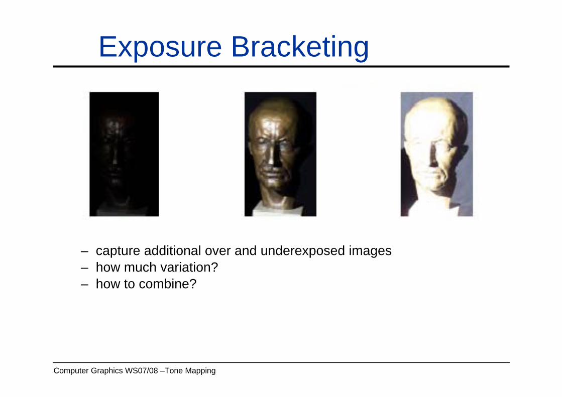
Exposure Bracketing
– capture additional over and underexposed images– how much variation? – how to combine?

Computer Graphics WS07/08 –Tone Mapping
Dynamic Range in Real World Images
– natural scenes: 18 stops (2^18)– human: 17stops
(after adaptation 30stops ~ 1:1,000,000,000)– camera: 10-16stops
[Stumpfel et al. 00]
Computer Graphics WS07/08 –Tone Mapping
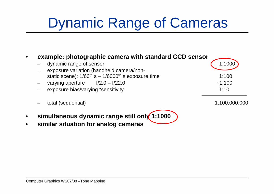
Dynamic Range of Cameras
• example: photographic camera with standard CCD sensor– dynamic range of sensor 1:1000– exposure variation (handheld camera/non-
static scene): 1/60th s – 1/6000th s exposure time 1:100– varying aperture f/2.0 – f/22.0 ~1:100– exposure bias/varying “sensitivity” 1:10
– total (sequential) 1:100,000,000
• simultaneous dynamic range still only 1:1000• similar situation for analog cameras

Computer Graphics WS07/08 –Tone Mapping
High Dynamic Range (HDR) Imaging
• basic idea of multi-exposure techniques:– combine multiple images with different
exposure settings– makes use of available sequential
dynamic range• other techniques available (e.g.
HDR video)
Computer Graphics WS07/08 –Tone Mapping
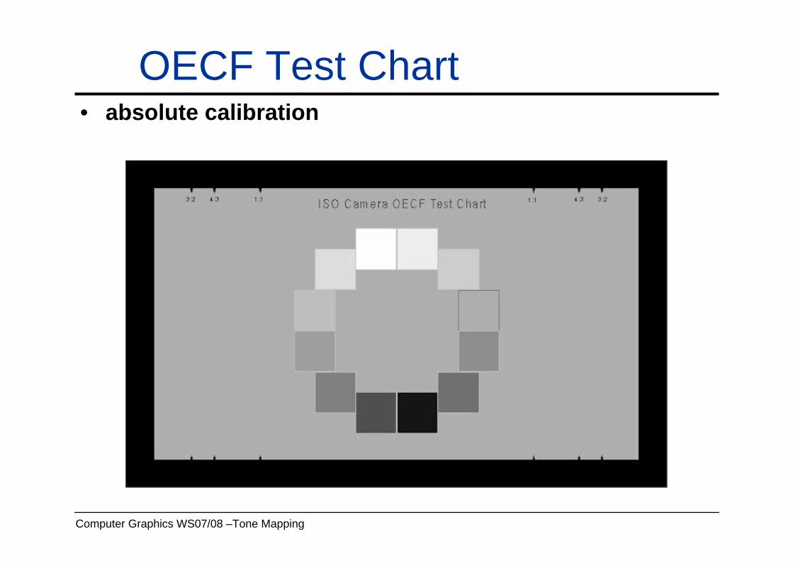
OECF Test Chart• absolute calibration
Computer Graphics WS07/08 –Tone Mapping
High Dynamic Range Imaging
– limited dynamic range of cameras is a problem• shadows are underexposed• bright areas are overexposed• sampling density is not sufficient
– some modern CMOS imagers have a higher and often sufficient dynamic range than most CCD imagers

Computer Graphics WS07/08 –Tone Mapping
High Dynamic Range (HDR) Imaging
– analog film with several emulsions of different sensitivity levels by Wyckoff in the 1960s
• dynamic range of about 108
– commonly used method for digital photography by Debevec and Malik(1997)
• selects a small number of pixels from the images • performs an optimization of the response curve with a smoothness
constraint– newer method by Robertson et al. (1999)
• optimization over all pixels in all images

Computer Graphics WS07/08 –Tone Mapping
High Dynamic Range Imaging
general idea of High Dynamic Range (HDR) imaging:– combine multiple images with different exposure times
• pick for each pixel a well exposed image• response curve needs to be known• don’t change aperture due to different depth-of-field

Computer Graphics WS07/08 –Tone Mapping
High Dynamic Range Imaging
Computer Graphics WS07/08 –Tone Mapping
HDR Imaging [Robertson et al.99]
Principle of this approach:Principle of this approach:•• calculate a HDR image using the response curvecalculate a HDR image using the response curve•• find a better response curve using the HDR imagefind a better response curve using the HDR image
(to be iterated until convergence)(to be iterated until convergence)
Computer Graphics WS07/08 –Tone Mapping
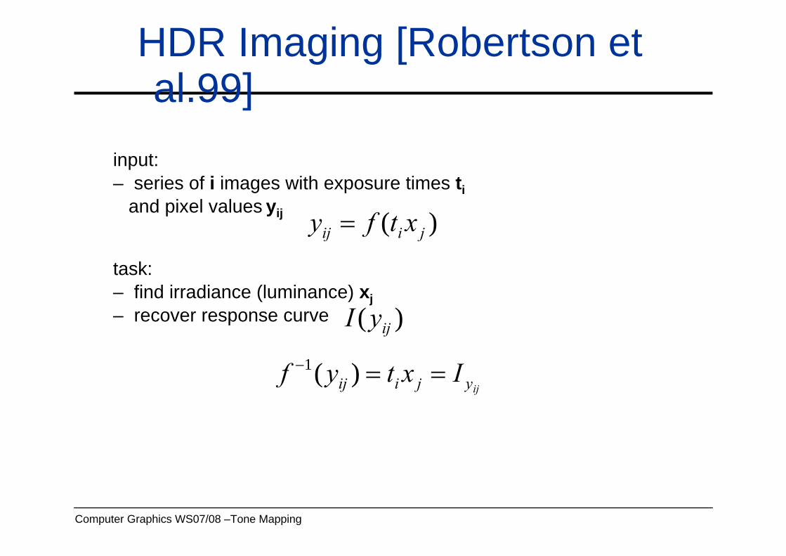
HDR Imaging [Robertson et al.99]
input:– series of i images with exposure times ti
and pixel values yij
task: – find irradiance (luminance) xj– recover response curve
)( jiij xtfy =
ijyjiij Ixtyf ==− )(1
)( ijyI

Computer Graphics WS07/08 –Tone Mapping
HDR Imaging [Robertson et al.99]
input:– series of i images with exposure times ti and pixel values yij– a weighting function wij = wij(yij) (bell shaped curve)– a camera response curve
• initial assumption: linear response ⇒calculate HDR values xj from images using
∑∑
=
iiij
iyiij
j tw
Itwx
ij
2
)( ijyI

Computer Graphics WS07/08 –Tone Mapping
HDR Imaging [Robertson et al.99]
optimizing the response curve resp. :– minimization of objective function O
using Gauss-Seidel relaxation yields
– normalization of I so that I128=1.0
2
,
)( jiji
yij xtIwOij−=∑
}:),{()(Card
1,
myjiE
xtE
I
ijm
Ejiji
mm
m
==
= ∑∈
)(mI)( ijyI
Computer Graphics WS07/08 –Tone Mapping
HDR Imaging [Robertson et al.99]
both steps– calculation of a HDR image using I– optimization of I using the HDR imageare now iterated until convergence
• criterion: decrease of O below some threshold• usually about 5 iterations
Computer Graphics WS07/08 –Tone Mapping
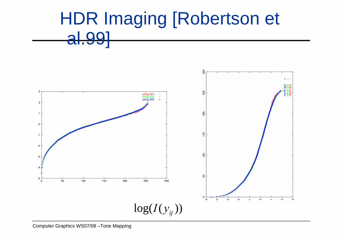
HDR Imaging [Robertson et al.99]
))(log( ijyI
Computer Graphics WS07/08 –Tone Mapping
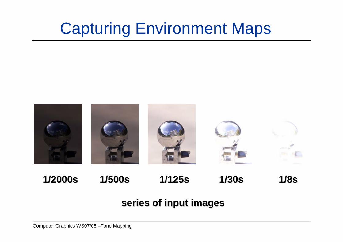
Capturing Environment Maps
1/2000s 1/500s 1/125s 1/30s 1/2000s 1/500s 1/125s 1/30s 1/8s 1/8s
series of input imagesseries of input images

Computer Graphics WS07/08 –Tone Mapping
series of input imagesseries of input images
Capturing Environment Maps

Computer Graphics WS07/08 –Tone Mapping
• [Robertson et al.99]
• choice of weighting function w(yij) for response recovery
– for 8 bit images– possible correction at both ends (over/underexposure)– motivated by general noise model
Weighting Function
⎟⎟⎠
⎞⎜⎜⎝
⎛ −−= 2
2
5.127)5.127(
4exp ijij
yw
Computer Graphics WS07/08 –Tone Mapping
• discussion– method very easy– doesn’t make assumptions about response curve shape– converges fast– takes all available input data into account– can be extended to >8 bit color depth– 16bit should be followed by smoothing
Algorithm of Robertson et al.
Computer Graphics WS07/08 –Tone Mapping
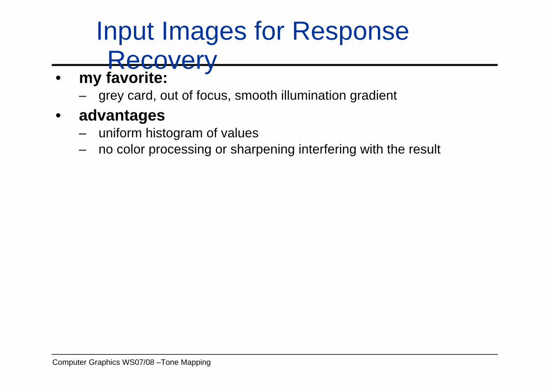
Input Images for Response Recovery
• my favorite:– grey card, out of focus, smooth illumination gradient
• advantages– uniform histogram of values– no color processing or sharpening interfering with the result

Computer Graphics WS07/08 –Tone Mapping
Input Images for HDR Generation
• how many images are necessary to get good results?– depends on scene dynamic range and on quality requirements– most often a difference of two stops (factor of 4) between exposures
is sufficient– [Grossberg & Nayar 2003]
Computer Graphics WS07/08 –Tone Mapping
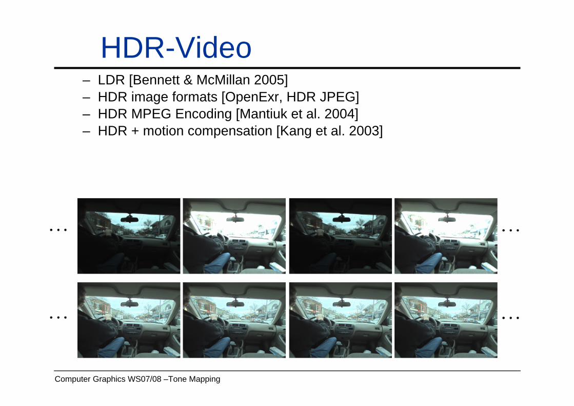
HDR-Video– LDR [Bennett & McMillan 2005]– HDR image formats [OpenExr, HDR JPEG]– HDR MPEG Encoding [Mantiuk et al. 2004]– HDR + motion compensation [Kang et al. 2003]
Computer Graphics WS07/08 –Tone Mapping
Tone-Mapping
Computer Graphics WS07/08 –Tone Mapping
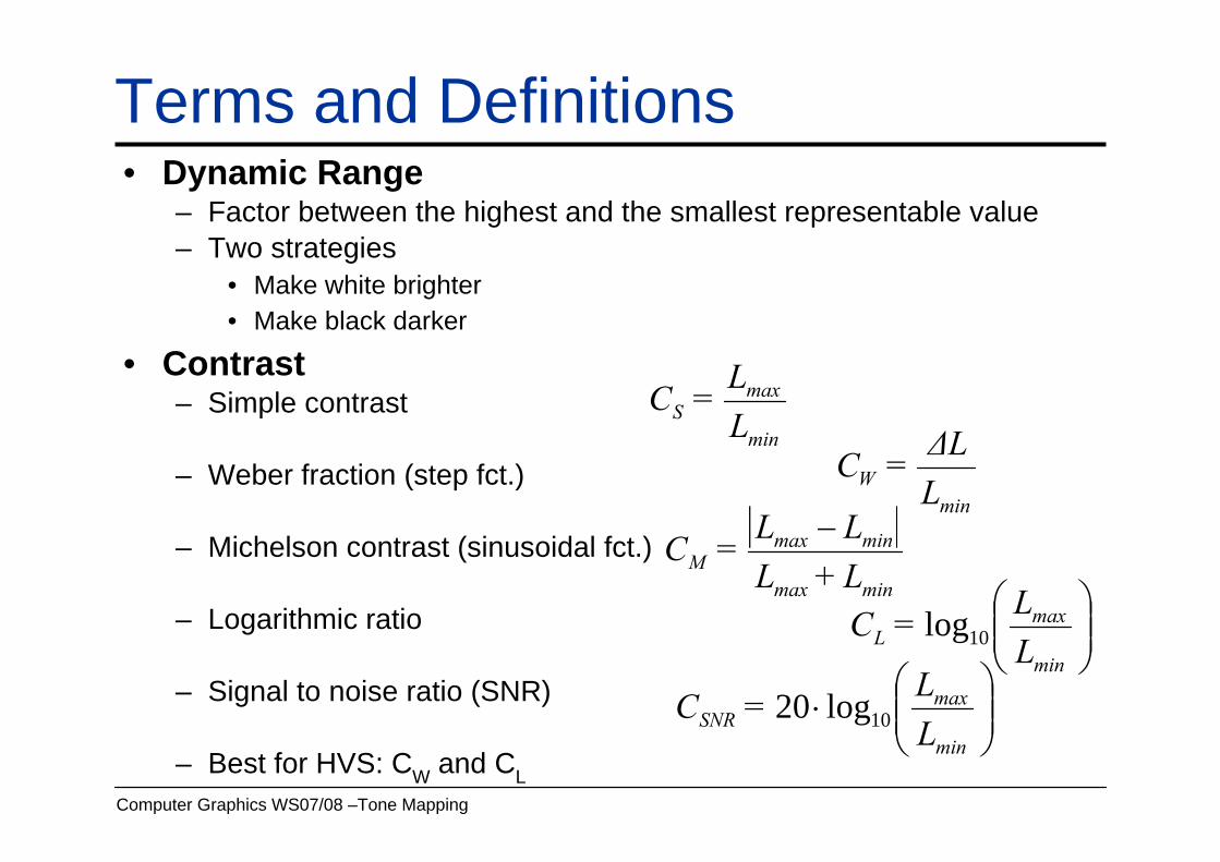
Terms and Definitions• Dynamic Range
– Factor between the highest and the smallest representable value– Two strategies
• Make white brighter• Make black darker
• Contrast– Simple contrast
– Weber fraction (step fct.)
– Michelson contrast (sinusoidal fct.)
– Logarithmic ratio
– Signal to noise ratio (SNR)
– Best for HVS: CW and CL
min
maxS L
L=C
| |minmax
minmaxM L+L
LL=C −min
W LΔL=C
⎟⎟⎠
⎞⎜⎜⎝
⎛
min
maxL L
L=C 10log
⎟⎟⎠
⎞⎜⎜⎝
⎛⋅
min
maxSNR L
L=C 10log20

Computer Graphics WS07/08 –Tone Mapping
Contrast Discrimination• Experiments [Whittle 1986]
– Including high contrast– Michelson does not work too well
• Particularly for high contrast– Good fits for CW and CL– Simplified linear model for CL
• ΔCL,simpl (CL) = 0.038737*CL0.537756
– [Mantiuk et al., 2006] CM
CLCW

Computer Graphics WS07/08 –Tone Mapping
Contrast Measurement• Contrast Detection Threshold
– Smallest detectable contrast in a uniform field of view• Contrast Discrimination Threshold
– Smallest visible difference between two similar signals– Works in the suprathreshold domain (signals above threshold)
• Often sinusoidal or square wave pattern
Computer Graphics WS07/08 –Tone Mapping
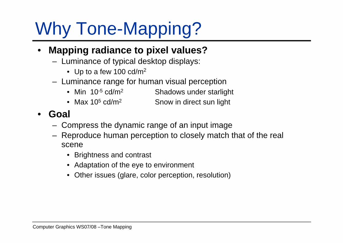
Why Tone-Mapping?• Mapping radiance to pixel values?
– Luminance of typical desktop displays:• Up to a few 100 cd/m2
– Luminance range for human visual perception• Min 10-5 cd/m2 Shadows under starlight• Max 105 cd/m2 Snow in direct sun light
• Goal– Compress the dynamic range of an input image– Reproduce human perception to closely match that of the real
scene• Brightness and contrast• Adaptation of the eye to environment• Other issues (glare, color perception, resolution)
Computer Graphics WS07/08 –Tone Mapping
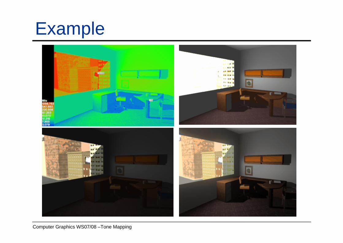
Example

Computer Graphics WS07/08 –Tone Mapping
Heuristic Approaches• Scaling brightest value to 1 (in gray value)
– Problem: light sources are often several orders of magnitude brighter than the rest
Rest will be black
• Scaling of brightest non-light-source value – Scaling to a value slightly below 1– Capping light source values to 1
• General problem of simple scaling– Absolute brightness gets lost:
• Dimming of light sources will have no effect
• Much better: Logarithmic domain– Linear scaling in the logarithmic domain
• Much closer to human perception– Typically using log10

Computer Graphics WS07/08 –Tone Mapping
General Principle• Approach [Tumblin/Rushmeier]
– Create model of the observer– Requirement:
• Observer should perceive same image from real and virtual display– Compute Tone-Mapping using concatenation and inversion of
operators– Model usually operates only on luminance (no color)

Computer Graphics WS07/08 –Tone Mapping
Maintaining Contrast• Contrast-based Scaling Factor [Ward `94]
– Maintain visible contrast differences in the image• Using Weber contrast
– Just noticeable contrast according to Blackwell [CIE`81](subjective measurements)
– La: Adaptation level of eye (luminance)
– Goal: linear scaling factor m(La)• Ld= m(La)Lw• Ld: display luminance• Lw: world luminance
5.24.0 )219.1(0594.0)( aa LLL +=Δ
Adaptation LAdaptation Laa [log cd/m[log cd/m22]]
ThresholdThresholdΔΔLL
[log cd/m[log cd/m22]]

Computer Graphics WS07/08 –Tone Mapping
Maintaining Contrast• Approach using „Just noticeable difference (JND)“
– Assume JND for real and virtual image are the same• JND of real world: ΔL(Lwa) • JND of display: ΔL(Lda)
– Substitution results in
– With Lda=Ldmax/2 and scaling factor sf in [0..1]
)()()( wawada LLLmLL Δ=Δ
5.2
4.0
4.0
219.1219.1)( ⎥
⎦
⎤⎢⎣
⎡++
=wa
dawa L
LLm
5.2
4.0
4.0max
max 219.1)2/(219.11
⎥⎥⎦
⎤
⎢⎢⎣
⎡
+
+=
wa
d
d LL
Lsf

Computer Graphics WS07/08 –Tone Mapping
Maintaining Contrast• Deriving Lwa
– Depends on light distribution in field of view of observer– Simple approximation using a single value
• Eyes try to adjust to average brightness• Brightness B:
log10(B)= a(Lin) log10(Lin) + b(Lin) Power-Law [Stevens`61]• Comfortable brightness
log10(Lwa)= E{log10(Lin)} + 0.84
• Problems of this Approach– Single factor for entire image
• Different adaptation for different locations in image• We do not perceive absolute differences in luminance
– Adaptation mainly acts on the 1 degree fov (fovea)– Results in clamping for too bright regions
Computer Graphics WS07/08 –Tone Mapping
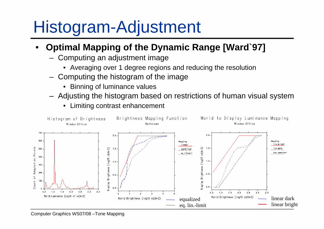
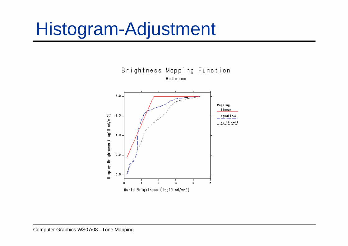
Histogram-Adjustment• Optimal Mapping of the Dynamic Range [Ward`97]
– Computing an adjustment image• Averaging over 1 degree regions and reducing the resolution
– Computing the histogram of the image• Binning of luminance values
– Adjusting the histogram based on restrictions of human visual system• Limiting contrast enhancement
linear darklinear bright
equalizedeq. lin.-limit

Computer Graphics WS07/08 –Tone Mapping
Histogram-Adjustment• Computing the Adjustment Image
– Assumes known view point– Average image
• Filtering non-overlapping regions covering 1 degree fov• Reference uses simple box filter

Computer Graphics WS07/08 –Tone Mapping
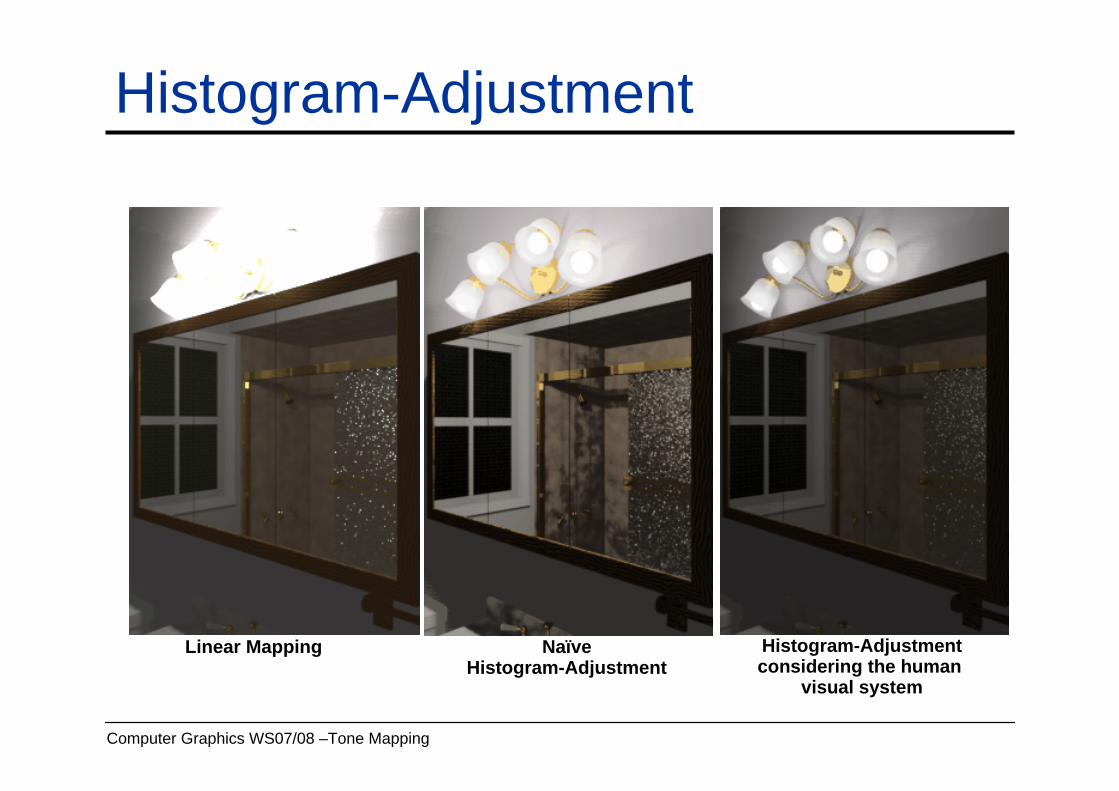
Histogram-Adjustment• Naïve Histogram Adjustment (Equalization)
– f(Bw): Number of sample per bin– P(Bw): Accumulated probability (sum of sample counts)– T: Sum over all f(Bw)– Mapping
)()]log()[log()log( minmaxmin wdddd BPLLLB −+=
Computer Graphics WS07/08 –Tone Mapping
Histogram-Adjustment
Linear Mapping NaïveHistogram-Adjustment
Histogram-Adjustmentconsidering the human
visual system

Computer Graphics WS07/08 –Tone Mapping
Histogram-Adjustment• Problem
– Too strong emphasis on contrast in highly populated regions of the dynamic range
– Idea:• Limiting the contrast enhancement (linear scaling works well for low
contrast images)
• Differentiate exp(Bd)= Ld with respect to Lw
leads to
w
d
w
d
w
w
d
d
LL
dLdL
LdL
LdL
≤⇒≤
)()]log()[log()log( minmaxmin wdddd BPLLLB −+=
w
d
w
ddwd
w
d
LL
LLL
bTBfB
dLdL
≤−
Δ=
)log()log()()exp( minmax

Computer Graphics WS07/08 –Tone Mapping
Histogram-Adjustment• Result
– Limiting the sample count per bin in histogram
– Implementation• Truncating too large bins with redistribution• Ditto without redistribution (gives better results)
)log()log()(
minmax ddw LL
bTBf−Δ
≤N
LLb
bfT
ww
i
)log()log(
)(
minmax −=Δ
=∑

Computer Graphics WS07/08 –Tone Mapping
Histogram-Adjustment• Implementing the Limitation
– Fails for cases where no compression is necessary• Can easily be detected
– Use modified f(Bw) in naïve histogram equalization
Computer Graphics WS07/08 –Tone Mapping
Histogram-Adjustment

Computer Graphics WS07/08 –Tone Mapping
Histogram-Adjustment• Adjustment for JND
– Limiting the contrast to the ratio of JNDs (global scale factor)
– That results in
– Implementation is the similar as for previous histogram limiting
)()(
wt
dt
w
d
LLLL
dLdL
ΔΔ
≤
ddd
w
wt
dtw LLL
bLTLLLLBf
)]log()[log()()()(
minmax −Δ
ΔΔ
≤

Computer Graphics WS07/08 –Tone Mapping
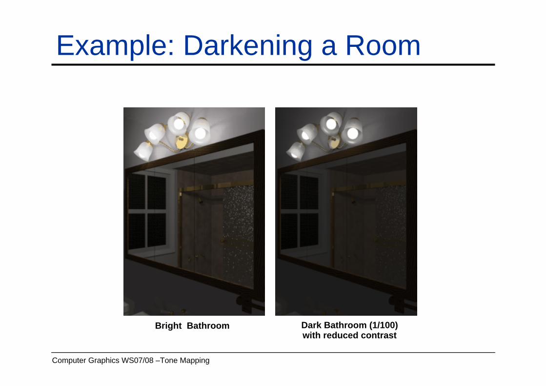
Example: Darkening a Room• Reduction in Contrast Sensitivity in Dark Scenes
Bright Bathroom Dark Bathroom (1/100)with reduced contrast
Computer Graphics WS07/08 –Tone Mapping
Example: Darkening a Room
Bright Bathroom Dark Bathroom (1/100)with reduced contrast

Computer Graphics WS07/08 –Tone Mapping
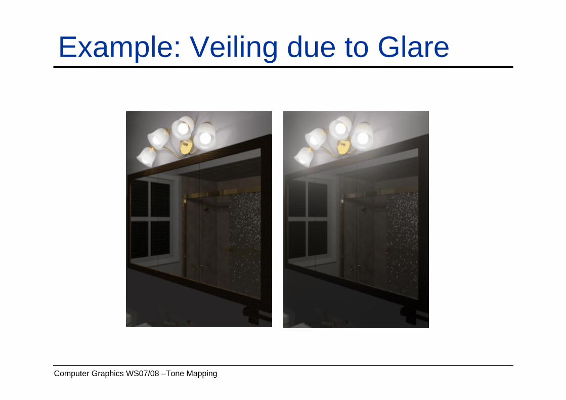
Extensions: Glare• Considering Glare
– Bright light sources result in veiling (German: Schleier)• Due to scattering of strong illumination in the eye
– Results in correction to adaptation level• Approach
– Moderate illumination in periphery does not contribute to adaptation• Depend exclusively on foveal region
– But: glare in the periphery does change the adaptation • Scattered light is added even in foveal region
– Compute a veiled image by filtering over peripheral region• Added to normal adaptation luminance Lf [Moon and Spencer,`45]
∫∫>
+=f
ddLKLL faθθ
φθθθθφθ
π)sin()cos(),(913.0 2
Computer Graphics WS07/08 –Tone Mapping
Example: Veiling due to Glare

Computer Graphics WS07/08 –Tone Mapping
Extensions• Loss of color vision in dark areas
• Loss of visual resolution in dark areas– Simple blur filter
Computer Graphics WS07/08 –Tone Mapping
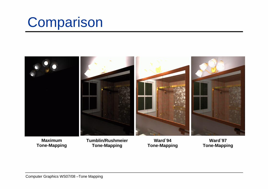
Comparison
MaximumTone-Mapping
Tumblin/RushmeierTone-Mapping
Ward`94Tone-Mapping
Ward`97Tone-Mapping

Computer Graphics WS07/08 –Tone Mapping
Comparison
Tumblin/RushmeierTone-Mapping
Ward`94Tone-Mapping
Ward`97Tone-Mapping
Computer Graphics WS07/08 –Tone Mapping
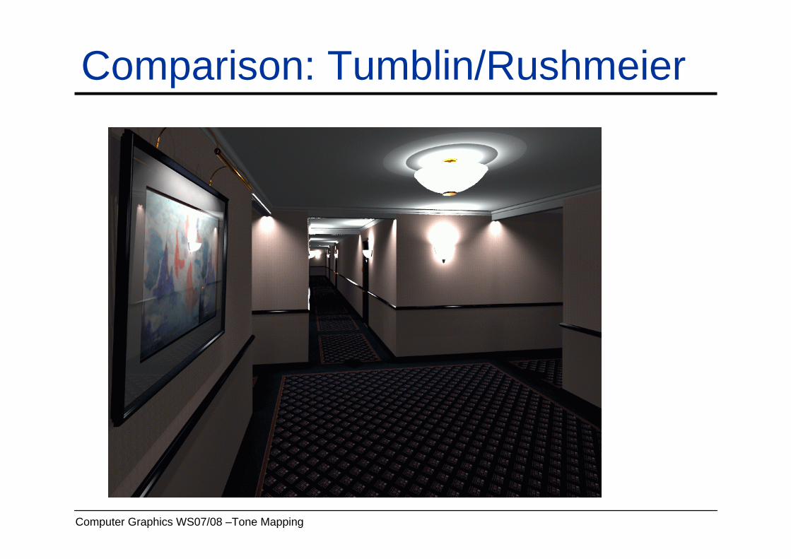
Comparison: Tumblin/Rushmeier

Computer Graphics WS07/08 –Tone Mapping
Comparison: Ward`94

Computer Graphics WS07/08 –Tone Mapping
Comparison: Ward`97

Computer Graphics WS07/08 –Tone Mapping
Local Tonemapping
• Usual contrast enhancement techniques– either enhance everything– or require manual intervention– change image appearance
• Tone mapping often gives numerically optimal solution– no dynamic range left for enhancement
tone mapping resultHDR image (reference)
restore missing contrast

Computer Graphics WS07/08 –Tone Mapping
Idea: Enhance Local Contrast
Reference HDR Image Tone Mapped Image
MeasureLost Contrast
at SeveralFeature Scales
EnhanceLost Contrast in
Tone Mapped Image
Enhanced TM Image
communicate lost image contents
maintain image appearance
[Krawczyk06]

Computer Graphics WS07/08 –Tone Mapping
Method: Adaptive Countershading
• Create apparent contrast based on Cornsweet illusion• Countershading
– gradual darkening / brightening towards a contrasting edge– contrast appears with ‘economic’ use of dynamic range
Enhanced Image
Computer Graphics WS07/08 –Tone Mapping
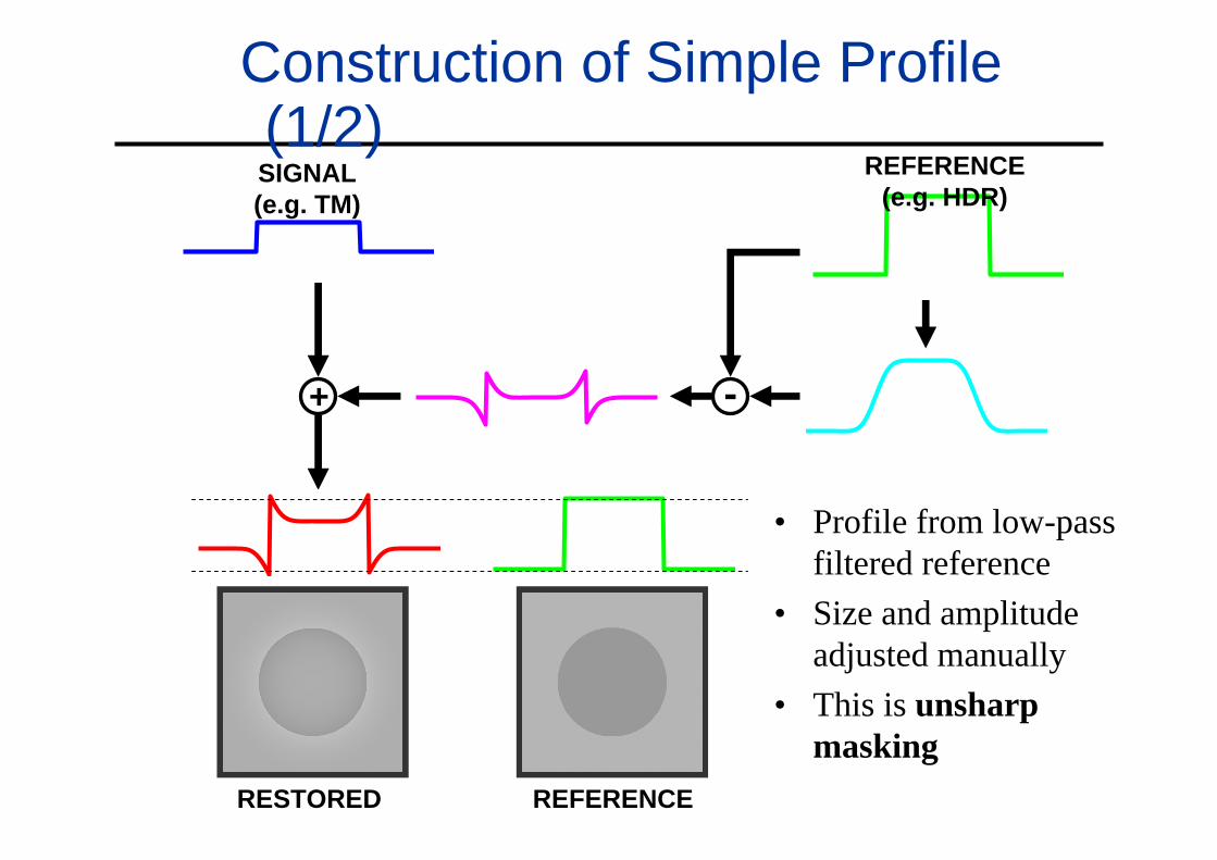
Construction of Simple Profile (1/2)SIGNAL(e.g. TM)
REFERENCE(e.g. HDR)
• Profile from low-pass filtered reference
• Size and amplitude adjusted manually
• This is unsharpmasking
-+
REFERENCERESTORED
Computer Graphics WS07/08 –Tone Mapping
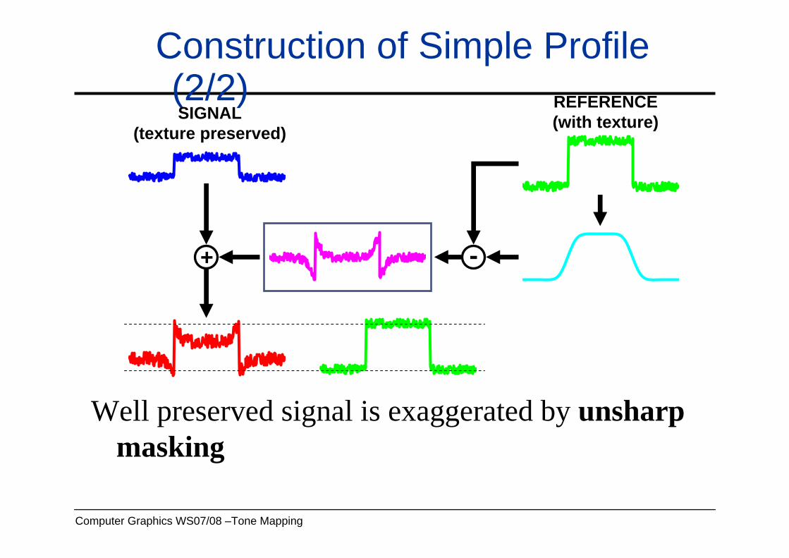
Construction of Simple Profile (2/2)SIGNAL
(texture preserved)
REFERENCE(with texture)
Well preserved signal is exaggerated by unsharpmasking
-+
Computer Graphics WS07/08 –Tone Mapping
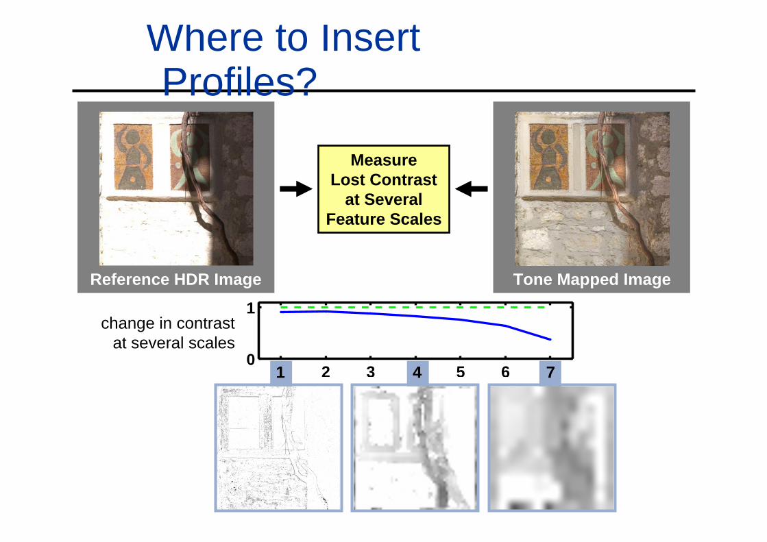
Where to Insert Profiles?
Reference HDR Image Tone Mapped Image
MeasureLost Contrast
at SeveralFeature Scales
1 2 3 4 5 6 70
1
1 4 7
change in contrastat several scales
Computer Graphics WS07/08 –Tone Mapping
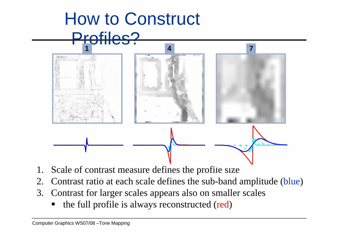
How to Construct Profiles?
1. Scale of contrast measure defines the profile size2. Contrast ratio at each scale defines the sub-band amplitude (blue)3. Contrast for larger scales appears also on smaller scales
the full profile is always reconstructed (red)
1 4 7
Computer Graphics WS07/08 –Tone Mapping
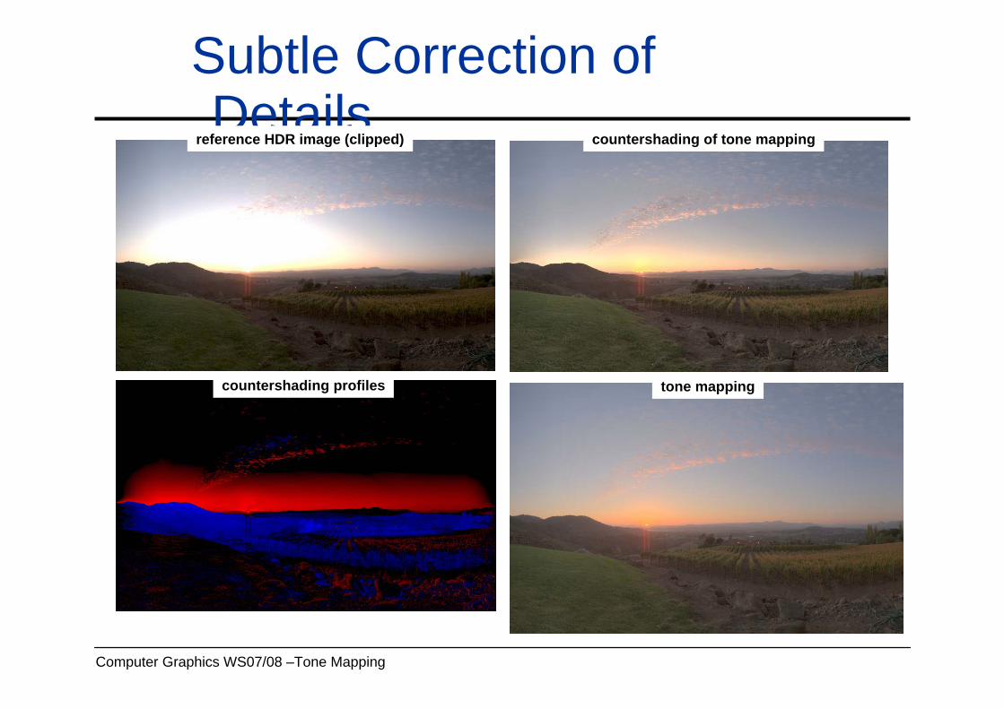
Subtle Correction of Details
reference HDR image (clipped) countershading of tone mapping
countershading profiles tone mapping
Computer Graphics WS07/08 –Tone Mapping
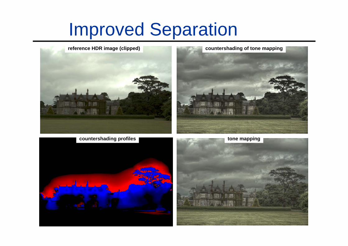
Improved Separationreference HDR image (clipped) countershading of tone mapping
countershading profiles tone mapping
Computer Graphics WS07/08 –Tone Mapping
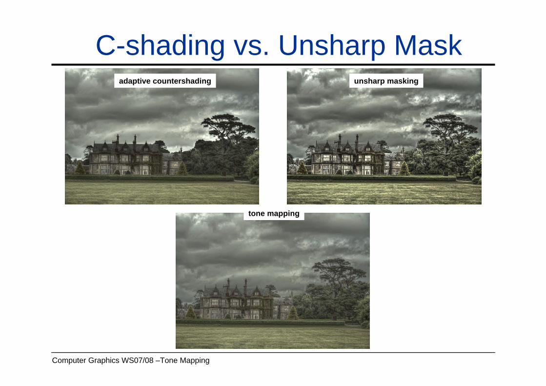
C-shading vs. Unsharp Mask
tone mapping
unsharp maskingadaptive countershading

Computer Graphics WS07/08 –Tone Mapping
Alternative: HDR Display• Human Visual System
– Sensitive to contrast, insensitive to absolute luminance difference– Mach bands: reduced resolution at discontinuities– “Very high contrast, although important on a global scale, cannot be
perceived by humans at high spatial frequencies”
• Idea [Heidrich et al., Siggraph 2004]– High-resolution transparency filter to modulate
high-intensity (low-resolution) image from a second display
– Transparency filter: LCD screen– High intensity image: video projector, array of superluminous LEDs– dynamic range: >50,000:1– maximum intensity: 2700 cd/m^2, 8500 cd/m^2

Computer Graphics WS07/08 –Tone Mapping
Setup
Computer Graphics WS07/08 –Tone Mapping
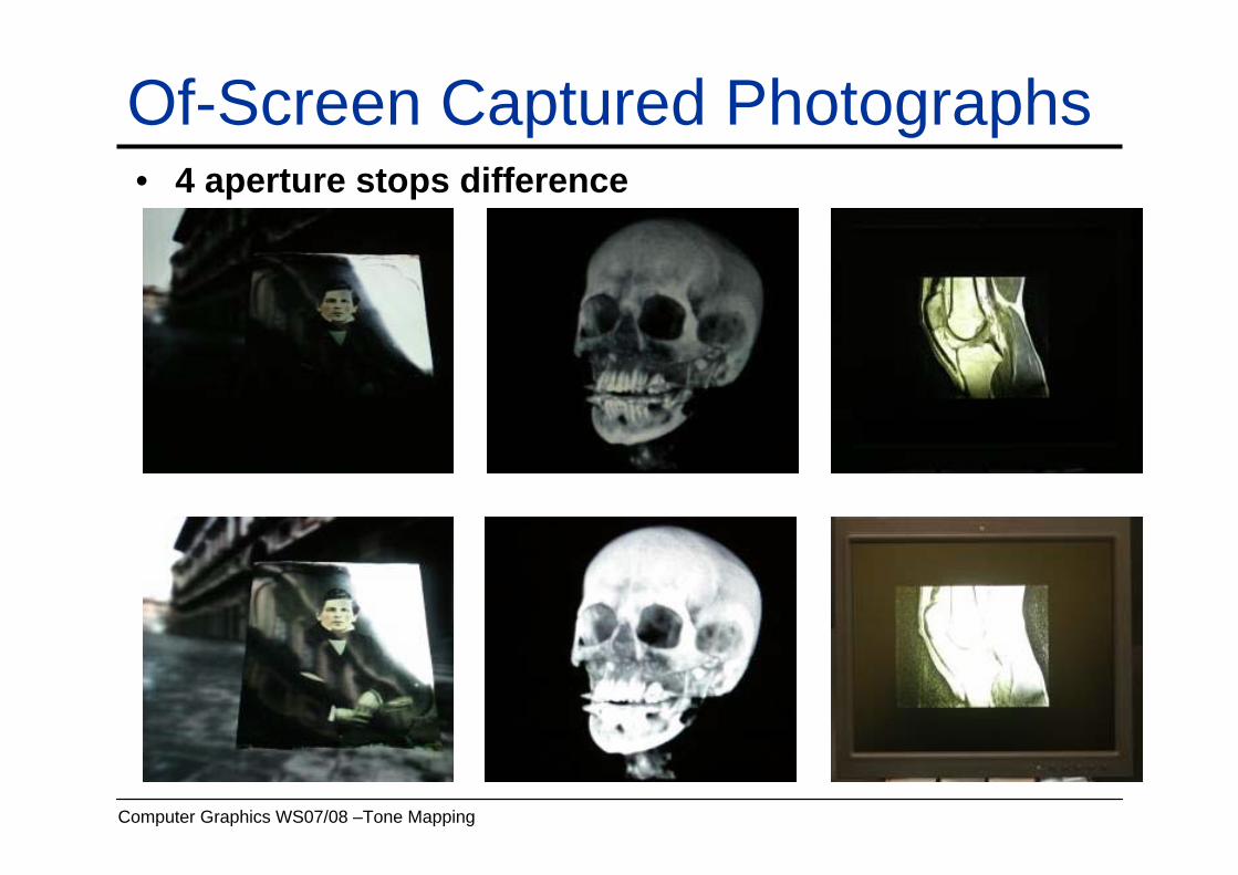
Of-Screen Captured Photographs• 4 aperture stops difference

Computer Graphics WS07/08 –Tone Mapping
Wrap-up• HDR acquisition• Tone mapping necessary due to dynamic range • Reduction of dynamic range• Histogram equalization• Just noticeable difference• HDR Display