1

Computer Architecture IITKT-3400 (TKT-3406)

Some remaining issues…

Jari NurmiTampere University of Technology

2006

Reliability, availability and dependability

• Dependability = the delivered service can be (justifiably) relied on

• Failure = actual behavior of the service different from specified behavior (an error affects the delivered service)

• Error = defect in module/system• Fault = cause for an error (first, a latent error until

activated)• Error latency = time difference of error

occurrence and the resulting failure

2

Reliability, availability and dependability

• Reliability = continuous service time, time to failure– e.g. MTTF (Mean Time To Failure) is a reliability measure– the reciprocal of MTTF = failure rate– collective failure rate of a system = sum of component

failure rates– service interruption time = MTTR (Mean Time To Repair)

• Availability = (for a non-redundant system) MTTF / (MTTF+MTTR)

• Reliability and availability are quantitative measures (unlike dependability)

Example• A disk subsystem has the following components and

MTTF– 10 disks, each 1,000,000 hours MTTF– 1 SCSI controller, 500,000-hour MTTF– 1 power supply, 200,000-hour MTTF– 1 fan, 200,000-hour MTTF– 1 SCSI cable, 1,000,000 MTTF

• Assuming independent failures, the MTTF for the system is– Failure rate 10 x 1/1M + 1/500,000 + 1/200,000 + 1/200,000 + 1/1M =

23/1M– MTTF = 1/Failure rate = 1M/23 = 43,500 hours (< 5 years)

• Assuming that the system will be serviced within 24 hours of the failure the availability is 43,500/43,524 = 99.94%

• Advertised ”five nines” availability (99.999%) of some computers would mean 5 minute down-time per year!

3

Reliability improvements• Fault avoidance = prevent fault occurrence by

construction• Fault tolerance = providing correct service by

adding redundancy• Error removal = minimization of latent errors by

verification (e.g. error correction codes)• Error forecasting = estimation of the presence,

creation and consequences of errors

Benchmarks of storage performance• Transaction-Processing Benchmarks

– simulation of order-entry environment» entering and delivering orders» recording payments» checking status of orders» monitoring stock at warehouses

– maintained by TPC, results audited• SPEC System-Level File Server (SFS)

– network file service (NFS) server synthetic benchmark• SpecWeb

– simulation of web accesses at a web server» mixture of small (icon) to very large (document) accesses

4

Benchmarks of dependability and availability

• In the TPC-C benchmark, there is a requirement that the system must handle a single disk failure (so, all are using some RAID configuration)

• Availability benchmarks only started to be constructed– measuring e.g. the policy and performance of RAID

reconstruction when a failure is injected– in the future also multiple fault recovery, other than RAID

system characterization, etc.

Network throughput and latency• Bisection bandwidth characterizes the network• The bandwidth to a single sender is often

referred to as throughput• Latency = sender overhead (e.g. checksum) +

time-of-flight + message size/throughput + receiver overhead (e.g. error correction)

• Time-of-flight = time for the message header to reach the receiver end

5

Network protocols

• TCP and IP headers:

• On-chip networks typically use simpler protocol stacks

Density-optimized processors?• Traditional desk-top processors are optimized to

performance (e.g. SPEC)• Power-efficiency becoming an important issue

also in non-portable devices– servers kept in collocation sites, where power causes a

major cost– the processor density is limited by the power consumption

(heat dissipation)• Replacing fewer power-hungry processors with

somewhat more power-efficient processors (a cluster) makes sense

6

Positioning the clusters...• Price/performance of SMP, NUMA and cluster

So, what have we learned on this course?

7

Architecture Trends in 1990’s-2000’s

• Address size doubling (32-bit to 64-bit)• Optimizing conditional branches by conditional (”predicated”)

execution– deep pipelining makes conditional branches costly– going to extend to greater degree of speculation

• Cache performance optimization via prefetch (Ch 5)• Support for multimedia• Faster floating-point operations (and merging FP to the core, not as

co-processor)• Long instruction words to gain more ILP (Ch 4)• Blending of DSP and general-purpose processors

– approaching from both sides• 80x86 emulation (like Transmeta Crusoe, see Ch 4)

MIPS with Tomasulo’s algorithm

8

• Solution: 2-bit scheme where prediction is changed only if mispredicted twice:

• Can be implemented as a saturating counter• 2-bit predictors do almost as well as n-bit predictors

2-bit Branch Prediction Buffer

T

T

NT

Predict Taken

Predict Not Taken

Predict Taken

Predict Not Taken

11 10

01 00T

NT

T

NT

NT

Branch Correlation Using Branch History

Two schemes (a, k, m, n)

• PA: Per address history, a > 0• GA: Global history, a = 0

n-bit saturating Up/DownCounter Prediction

Table size (usually n = 2): #bits = k * 2a + 2k * 2m *n

Variant: Gshare (Scott McFarling’93): GA which takes logic OR of PC address bits and branch history bits

Branch Address0 1 2k-1

0

1

2m-1

Branch History Table

a k

m

Pattern History Table

9

Tournament predictors• One form of multilevel branch predictors• Several (≥2) levels of branch prediction

tables + algorithm to ”predict the right predictor”

• E.g., local and global • In Alpha 21264

– 4k 2-bit counters indexed by local branch address to select between global/local

– 4k 2-bit counters indexed by last 12 branches

– two-level local predictor» 1k 10-bit history table (10 last branches at the local

address)» indexes 1k 3-bit counters

– total 29k bits– less than 1/1000 mispredictions

(SPECfp95)!!!

A 2-bit saturating counterselects the predictor.

Branch Target Buffer• Branch condition is not enough !!• High-bandwidth instruction stream needed• Branch Target Buffer (BTB): Tag and Target address

Tag branch PC PC if taken

=? Branchprediction(often in separatetable)

Yes: instruction is branch. Use predicted PC as next PC if branch predicted taken.No: instruction is not a

branch. Proceed normally

10…..10 101 00PC

10

Superscalar ConceptInstructionMemory

InstructionCache

Decoder

BranchUnit ALU-1 ALU-2 Logic &

ShiftLoadUnit

StoreUnit

ReorderBuffer Register

File

DataCache

DataMemory

Reservation Stations

Address

DataData

Instruction

Key ideas of speculation• Instructions may execute out-of-order but are forced to

commit in order• Instruction commit happens when the instruction is no

longer speculative (the prediction was proven correct)• Buffer needed to hold instructions that have executed but

not committed: Re-Order Buffer (ROB)• ROB is also used to pass results among instructions

(maybe speculated)• ROB is like the store buffer and can also take care of its

functionality• ROB entry: instruction type (branch/store/ALU), destination

(reg/memory address), value, ready

11

MIPS FP unit extended

Hardware speculation features• In-order commit allows precise interrupts! (ROB acts as a

future file)• If speculated instruction raises an exeption, it is recorded in

ROB; if misprediction flushed; if correct take exception before finally committing the instruction

• Memory writes do not happen until the store instruction is no more speculative!

• In-order commit also resolves WAW and WAR hazards• RAW hazards need two restrictions: not allowing load if an

active ROB store entry points to the same address and maintaining program order in effective address calculation (load address only after all preceding stores)

12

35

41

16

5860

9

1210

48

15

67 6

46

13

45

6 6 7

45

14

45

2 2 2

29

4

19

46

0

10

20

30

40

50

60

gcc espresso li fpppp doducd tomcatv

Program

Inst

ruct

ion

issu

es p

er c

ycle

Perfect Selective predictor Standard 2-bit Static None

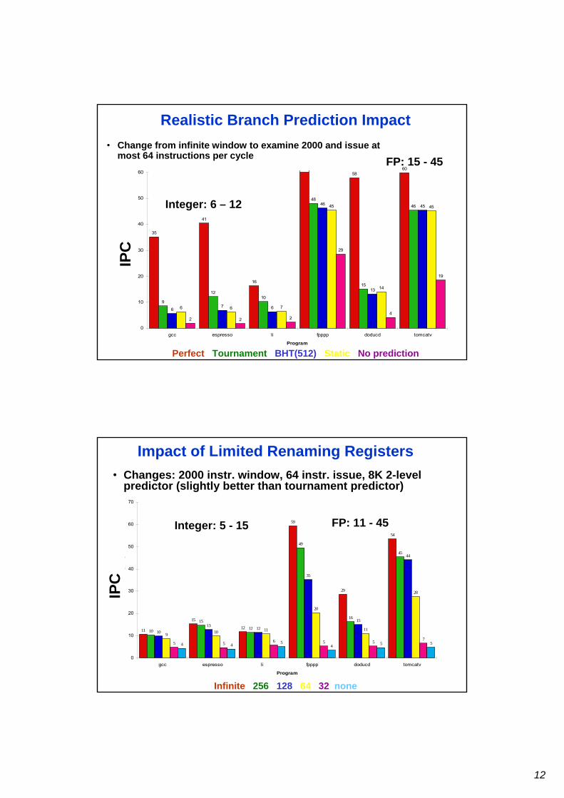
Realistic Branch Prediction Impact• Change from infinite window to examine 2000 and issue at

most 64 instructions per cycle FP: 15 - 45

Integer: 6 – 12

IPC

Perfect Tournament BHT(512) Static No prediction

11

15

12

29

54

10

15

12

49

16

1013

12

35

15

44

9 10 11

20

11

28

5 5 6 5 57

4 4 54 5 5

59

45

0

10

20

30

40

50

60

70

gcc espresso li fpppp doducd tomcatv

Program

Inst

ruct

ion

issu

es p

er c

ycle

Infinite 256 128 64 32 None

Impact of Limited Renaming Registers• Changes: 2000 instr. window, 64 instr. issue, 8K 2-level

predictor (slightly better than tournament predictor)

Integer: 5 - 15 FP: 11 - 45

IPC

Infinite 256 128 64 32 none

13

Program

0

5

10

15

20

25

30

35

40

45

50

gcc espresso li fpppp doducd tomcatv

10

15

12

49

16

45

7 79

49

16

45 4 4

6 53

53 3 4 4

45

Perfect Global/stack Perfect Inspection None

Memory Address Alias Impact• Changes: 2000 instr. window, 64 instr. issue, 8K 2-

level predictor, 256 renaming registers

FP: 4 - 45(Fortran,no heap)

Integer: 4 - 9

IPC

Perfect Global/stack perfect Inspection None

Program

0

10

20

30

40

50

60

gcc expresso li fpppp doducd tomcatv

10

15

12

52

17

56

10

15

12

47

16

10

1311

35

15

34

910 11

22

12

8 8 9

14

9

14

6 6 68

79

4 4 4 5 46

3 2 3 3 3 3

45

22

Infinite 256 128 64 32 16 8 4

Window Size Impact• Assumptions: Perfect disambiguation, 1K tournament predictor, 16 entry return

stack, 64 renaming registers, issue as many as window

Integer: 6 - 12

FP: 8 - 45

IPC

14

Multiple-Issue Processors

• Vector Processing: Explicit coding of independent loops as operations on large vectors of numbers– Multimedia instructions being added to many processors

• Multiple-Issue Processors– Superscalar: varying no. instructions/cycle (1 to 8), scheduled by

compiler or by HW (Tomasulo) (dynamic issue capability)» IBM PowerPC, Sun UltraSparc, DEC Alpha, Pentium III/4

– VLIW (very long instr. word): fixed number of instructions (4-16) scheduled by the compiler (static issue capability)» Intel Architecture-64 (IA-64), TriMedia, TI C6x

• Anticipated success of multiple instructions led to Instructions Per Cycle (IPC) metric instead of CPI

Architecture ComparisonCharacteristic CISC RISC VLIWInstruction size varies one size one sizeInstr. format field placement regular regular

variesInstr. semantics varies from simple one simple many simple

to complex operation operationsRegisters few, sometimes many, GP many, GP

specialHardware design Microcoded Impl. with Impl. with

implementations one pipeline multiple pipe

Pic. of 5 instr

15

Superscalar versus VLIW• VLIW advantages:

– Much simpler to build. Potentially faster

• VLIW disadvantages and proposed solutions:– Binary code incompatibility

» Object code translation or emulation» Less strict approach (EPIC, IA-64, Itanium)

– Increase in code size, unfilled slots are wasted bits» Use clever encodings, only one immediate field» Compress instructions in memory and decode them when they are fetched

– Lockstep operation: if the operation in one instruction slot stalls, the entire processor is stalled» Less strict approach

Advanced compiler support techniques

• Loop-level parallelism• Software pipelining• Global scheduling (across basic blocks)

16

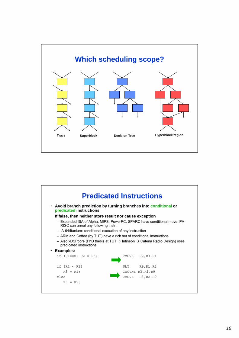
Which scheduling scope?

Trace Superblock Decision Tree Hyperblock/region

• Avoid branch prediction by turning branches into conditional or predicated instructions:If false, then neither store result nor cause exception– Expanded ISA of Alpha, MIPS, PowerPC, SPARC have conditional move; PA-

RISC can annul any following instr.– IA-64/Itanium: conditional execution of any instruction– ARM and Coffee (by TUT) have a rich set of conditional instructions– Also xDSPcore (PhD thesis at TUT Infineon Catena Radio Design) uses

predicated instructions• Examples:

if (R1==0) R2 = R3; CMOVZ R2,R3,R1

if (R1 < R2) SLT R9,R1,R2

R3 = R1; CMOVNZ R3,R1,R9

else CMOVZ R3,R2,R9

R3 = R2;

Predicated Instructions

17

Speculative Loads• Speculative load (sld): does not generate exceptions• Speculation check instruction (specck): check for

exception. The exception occurs when this instruction is executed. Exact exception behavior is preserved.

ld r1,0(r3) # load A

sld r9,0(r2) # speculative load B

bnez r1,L1 # test A

specck 0(r2) # perform exception check

j L2

L1: addi r9,r1,4 # else part

L2: st r9,0(r3) # store A

Using poison bit• Exception tracked when occuring but any

terminating exception is postponed until the result is used. Not completely precise exception.

• Speculative load turns on the poison bit, normal use (addi) turns it off:

ld r1,0(r3) # load A

sld r14,0(r2) # speculative load B

beqz r1,L3 # test A

addi r14, r1, 4 # else part

L3: st r14,0(r3) # store A

18

EPIC Architecture: IA-64• Instructions grouped in 128-bit bundles

– 3 * 41-bit instruction– 5 template bits, indicate type and stop location

• Each 41-bit instruction – starts with 4-bit opcode, and – ends with 6-bit guard (boolean) predicate register-id

Predication and speculation support in IA-64• Nearly all instructions can be predicated• Predicate registers set by compare or test

– Ten different tests– Two predicate registers as target

» Result and its complement» Logical function output of two tests (and its complement)

• Poison bits (NaT = Not a Thing bits) used for deferred exceptions• NaTVal floating-point value encoded in the FP result register• In addition to causing an exception when the NaT/NaTVal is used, there

are explicit checks• Speculative and non-speculative loads• Advanced load for speculating; creates ALAT table entry with load

destination register and memory address– Stores check against the ALAT entries and invalidate the entry if the addresses

match

19

TriMedia TM32• Classic VLIW with 5 parallel operations, relies

fully on the compiler to avoid hazards• 23 functional units of 11 types, restricted

combinations of 5 operations in one instruction• Each individual operation predicated with a

single register value; if 0 cancel• At most 1 branch with true predicate in an

instruction (compiler must take care)• Speed-optimized code size about 4x compared to

MIPS, performance/clock rate about 12x

Instruction coding in xDSPcore• Instruction: one or two instruction words

• Execution bundle: xLIW = scalable long instruction word

• Fetch bundle: four instruction words

20 bit

40 bit

from 1 instruction up to10 instructions words ...

20

Instruction fetch and issue in xDSPcore

• 1 to 5 instructions (1 to 10 instruction words) executed in parallel

INS 1INS 1 INS 2INS 2 INS 3INS 3 INS 4INS 4

INS 5INS 5 INS 6INS 6 INS 7INS 7 INS 8INS 8

INS 9INS 9 INS10INS10 INS11INS11 INS 12INS 12

Align Unit

INS 1INS 1 INS 2INS 2

INS 3INS 3 INS 4INS 4 INS 5INS 5 INS 6INS 6

INS 7INS 7

INS 8INS 8 INS 9INS 9

INS 10INS 10 INS 11INS 11 INS 12INS 12

MOV1MOV1 MOV2MOV2 CMP1CMP1 CMP2CMP2 BRBR

Transmeta Crusoe• VLIW for low-power portable computing• Two- and four-operation instructions (64/128-bit)• Five types of operation slots: ALU, Compute, Memory, Branch,

Immediate• Software emulation of x86 instruction set

– Interpretation instruction-by-instruction– Translation of basic blocks to Crusoe code sequence (and caching)

• Support for reordering– Shadowed register file– Program-controlled store buffer– Memory alias detection hardware with speculative loads– Conditional move instruction

• Permanent state is not changed until no exceptions possible (shadow registers, store buffer)

• Precise state of x86 instructions execution in shadow registers• Also speculative stores (to the store buffer only)

21

Direct mapped and associative caches

Tag Data Tag Data Tag Data Tag Data Tag Data Tag Data Tag Data Tag Data

Eight-way set associative (fully associative)

Tag Data Tag Data Tag Data Tag Data

Four-way set associative

Set

0

1

Tag Data

One way set associative�(direct mapped)

Block

0

7

1

2

3

4

5

6

Tag Data

Two-way set associative

Set

0

1

2

3

Tag Data

block

2 blocks / set

4 blocks / set

8 blocks / set

• Taking advantage of spatial locality:

Direct Mapped Cache

Address (showing bit positions)

16 12 Byte�offset

V Tag Data

Hit Data

16 32

4K�entries

16 bits 128 bits

Mux

32 32 32

2

32

Block offsetIndex

Tag

31 16 15 4 3 2 1 0

Address (bit positions)

22

A 4-Way Set-Associative Cache

2 2 8

V TagIndex012

25 325 425 5

D ata V Ta g D a ta V T ag D ata V T ag D ata

3 22 2

4 - to - 1 m ultip le xo r

H it D a ta

1238910111 23 031 0

Set 2

Way 3

2nd Way to Reduce Miss Penalty: Subblock Placement

• Don’t have to load full block on a miss• Have valid bits per sub-block to indicate valid• (Originally invented to reduce tag storage)

Valid Bits Subblocks

1 1 1 11 1 0 00 1 0 10 0 0 0

100300200204

Tags

23

3rd Way to Reduce Miss Penalty: Early Restart and Critical Word First

• Don’t wait for full block to be loaded before restarting CPU– Early restart—As soon as the requested word of the block

arrives, send it to the CPU and continue– Critical Word First—Request the missed word first from

memory and send it to the CPU as soon as it arrives; let the CPU continue while filling the rest of the words in the block

• Generally useful only when blocks are large

4th Way to Reduce Miss Penalty:Add a Victim Cache

• How to combine fast hit time of direct-mapped cache yet avoid conflict misses?

• Add a small fully associative cache in which replaced blocks are given a “second chance”

• Jouppi [1990]: 4-entry victim cache removed 20% to 95% of conflict misses for a 4 KB direct-mapped data cache

• Used in Alpha, HP machines

24

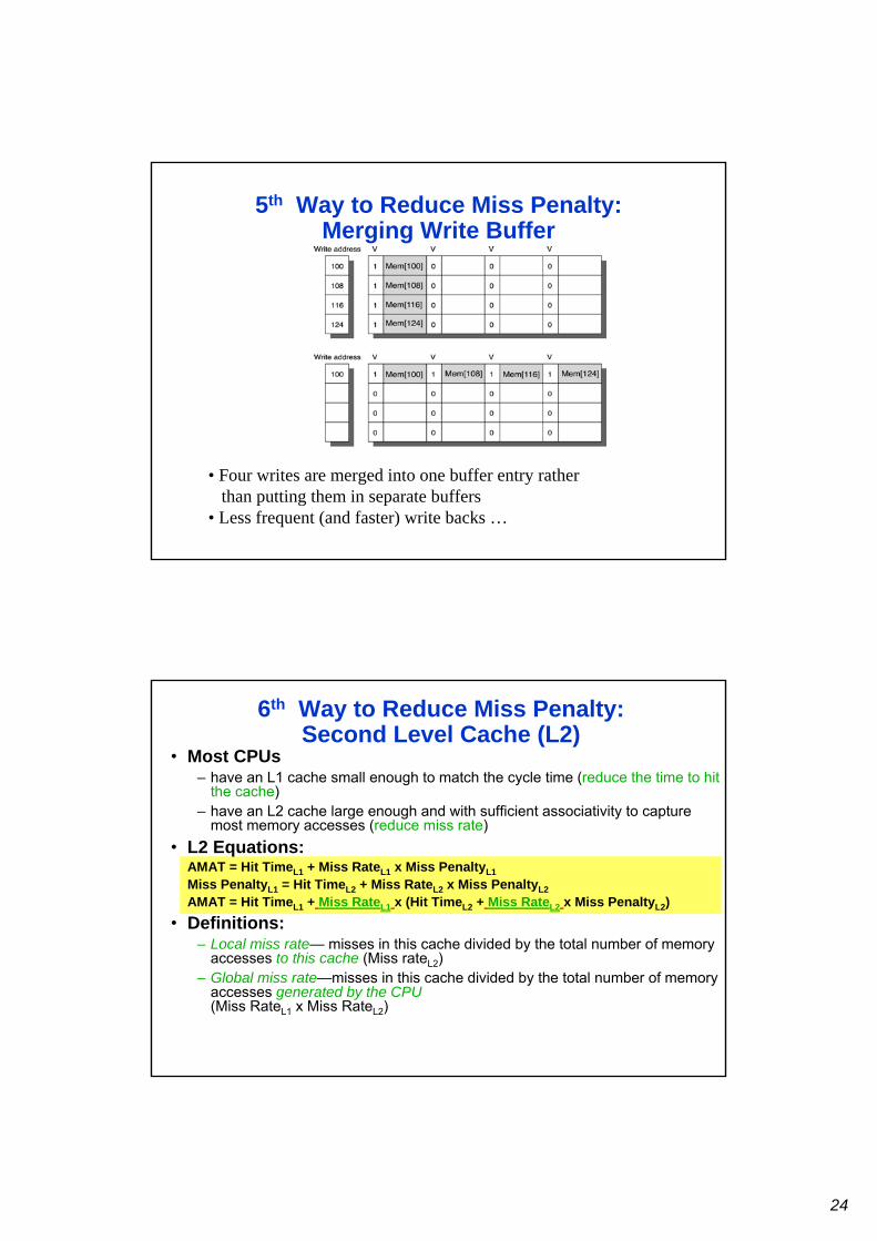
5th Way to Reduce Miss Penalty:Merging Write Buffer

• Four writes are merged into one buffer entry rather than putting them in separate buffers

• Less frequent (and faster) write backs …

6th Way to Reduce Miss Penalty:Second Level Cache (L2)

• Most CPUs– have an L1 cache small enough to match the cycle time (reduce the time to hit

the cache)– have an L2 cache large enough and with sufficient associativity to capture

most memory accesses (reduce miss rate)• L2 Equations:

AMAT = Hit TimeL1 + Miss RateL1 x Miss PenaltyL1Miss PenaltyL1 = Hit TimeL2 + Miss RateL2 x Miss PenaltyL2AMAT = Hit TimeL1 + Miss RateL1 x (Hit TimeL2 + Miss RateL2 x Miss PenaltyL2)

• Definitions:– Local miss rate— misses in this cache divided by the total number of memory

accesses to this cache (Miss rateL2)– Global miss rate—misses in this cache divided by the total number of memory

accesses generated by the CPU(Miss RateL1 x Miss RateL2)

25

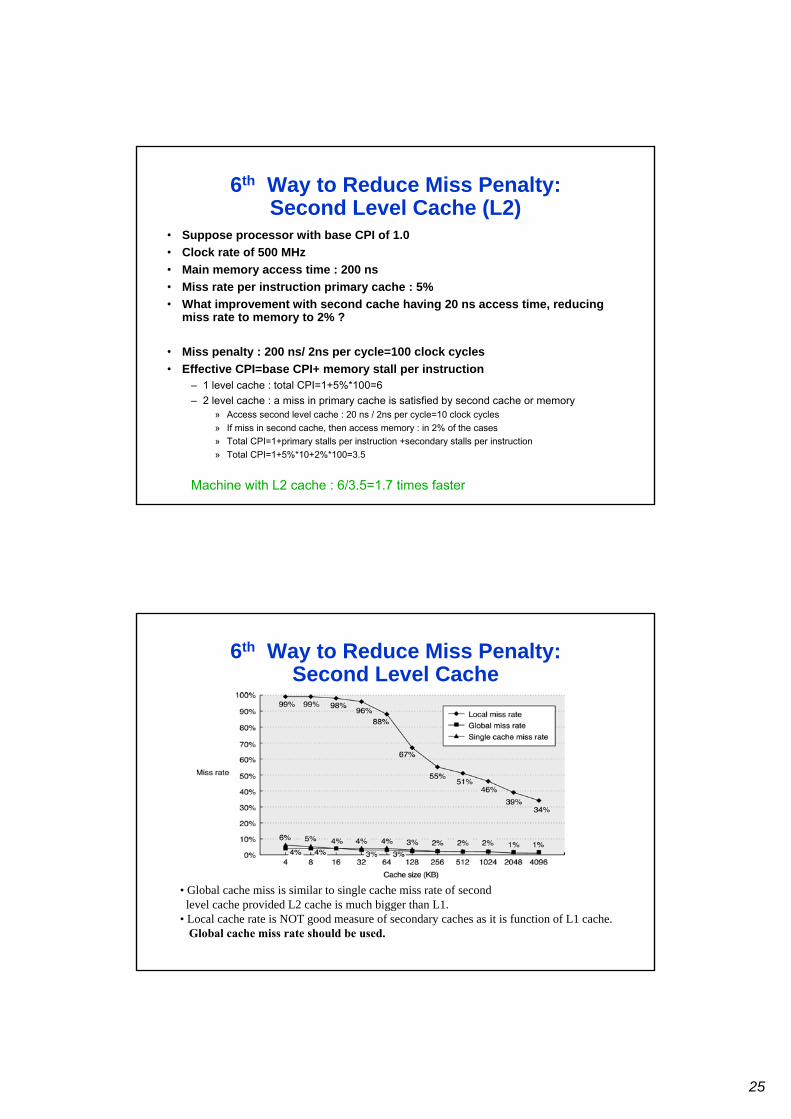
6th Way to Reduce Miss Penalty:Second Level Cache (L2)

• Suppose processor with base CPI of 1.0• Clock rate of 500 MHz• Main memory access time : 200 ns• Miss rate per instruction primary cache : 5%• What improvement with second cache having 20 ns access time, reducing

miss rate to memory to 2% ?

• Miss penalty : 200 ns/ 2ns per cycle=100 clock cycles• Effective CPI=base CPI+ memory stall per instruction

– 1 level cache : total CPI=1+5%*100=6– 2 level cache : a miss in primary cache is satisfied by second cache or memory

» Access second level cache : 20 ns / 2ns per cycle=10 clock cycles» If miss in second cache, then access memory : in 2% of the cases» Total CPI=1+primary stalls per instruction +secondary stalls per instruction» Total CPI=1+5%*10+2%*100=3.5

Machine with L2 cache : 6/3.5=1.7 times faster

6th Way to Reduce Miss Penalty:Second Level Cache

• Global cache miss is similar to single cache miss rate of second level cache provided L2 cache is much bigger than L1.

• Local cache rate is NOT good measure of secondary caches as it is function of L1 cache. Global cache miss rate should be used.

26

6th Way to Reduce Miss Penalty:Second Level Cache

Reducing Miss Penalty Summary

• Six techniques– Read priority over write on miss– Sub-block placement– Early Restart and Critical Word First on miss– Victim cache– Write buffer merging– Second Level Cache

• Can be applied recursively to Multilevel Caches– Danger is that time to DRAM will grow with multiple levels in

between

27

How Can We Reduce Misses?

• 3 Cs: Compulsory, Capacity, Conflict• In all cases, assume total cache size not changed

What happens if we1) Change Block Size:

Which of 3Cs is obviously affected? compulsory2) Change Cache Size:

Which of 3Cs is obviously affected? capacity misses3) Introduce higher associativity :

Which of 3Cs is obviously affected? conflict misses

Block Size (bytes)

Miss Rate

0%

5%

10%

15%

20%

25%

16 32 64

128

256

1K

4K

16K

64K

256K

1st Way to Reduce Misses:Increase Block Size

28

2nd way to reduce miss rate : Larger Caches

• Increase capacity of cache

• Disadvantages : – longer hit time (may determine processor cycle time!!)– higher cost

3rd Way to Reduce Misses:Increase Associativity

• 2:1 Cache Rule: – Miss Rate direct-mapped cache of size N ≈

Miss Rate 2-way set-associative cache of size N/2

• Beware: Execution time is only true measure of performance!– Access time of set-associative caches larger than access time direct-

mapped caches– L1 cache often direct-mapped (access must fit in one clock cycle)– L2 cache often set-associative (cannot afford to go to main memory)

29

• How to combine fast hit time of direct-mapped and have the lower conflict misses of 2-way SA cache?

• Divide cache in two halves. First check one half. If miss, check other half.• If in second half: pseudo-hit (slow hit)

• Note that two separate searches are conducted on a miss.• The first search proceeds as it would for direct-mapped cache.• Since there is no associative hardware, hit time is fast if it is found the first time.• Drawback: CPU pipeline is hard to design if hit takes 1 or 2 cycles

– Better for caches not tied directly to processor (L2)– Used in MIPS R1000 L2 cache, similar in UltraSPARC

4th Way to Reduce Misses:Pseudo-Associative Caches

Time

Hit Time

Pseudo Hit Time Miss Penalty

5th Way to Reduce Misses:Compiler Optimizations

• McFarling [1989] reduced caches misses by 75% for 8KB direct-mapped cache, 4-byte blocks in software

• Instructions– Reorder procedures in memory so as to reduce conflict misses– Profiling to look at conflicts (using developed tools)

• Data– Merging Arrays: improve spatial locality by single array of compound

elements vs. 2 arrays– Loop Interchange: change nesting of loops to access data in order

stored in memory– Loop Fusion: combine 2 independent loops that have same looping

and some variables overlap– Blocking: Improve temporal locality by accessing “blocks” of data

repeatedly vs. going down whole columns or rows

30

Hit Time Reduction Techniques• Small (must fit on-chip) and simple (direct-

mapped)• Avoid address translation

– Use virtual addresses for the cache (virtual cache vs. physical cache)

– Problem: cache needs to be flushed on a process switch or a process identifier (PID) must be added to the tag

• Pipelining writes– For reads, checking the tag and reading the data can be

performed in parallel, but not for writes

31

Reducing miss penalty or miss rate by introducing Parallellism

• Prefetching• Non blocking cache• Compiler controlled fetching

Bandwidth to main memory• Next level from cache(s) is the main memory• Characterized by latency and bandwidth• Very little can be done for latency• The bandwidth can be improved in different ways• Baseline performance:

– 4 clock cycles to send address– 56 clock cycles for the access of a word– 4 clock cycles to send a word of data

– Miss penalty for 4 word x 8 bytes blocks = 4x(4+56+4) = 256 cycles– Memory bandwidth 1/8 bytes per cycle (32/256)

32

Techniques to speed up memory

Caches and virtual memory – similarities and differences

• In most parts, caches and virtual memory are very analogous– block is called page or segment– miss is called page fault or address fault

• Virtual memory needs address translation• Operating system (SW) controls virtual memory replacements (HW in

caches)• Processor address size determines the size of virtual memory (cache

size is independent)• Secondary storage in virtual memory is also used for the file system

(not normally in the address space!)• Cache blocks and paged memory address straightforward to address,

segments need two addresses (segment number + offset)– segments seldom used in modern computers– paged segments and multiple page sizes instead (hybrid schemes)

33

Virtual to physical address mapping

• E.g. 32-bit address, 4 kB pages, 4 bytes per page table entry 4 MB table

• Inverted page table: storing virtual – physical pairs for all physical pages: 512 MB physical memory 8 x 512 M / 4k = 1 MB

TLB• Page tables in main memory

– two accesses: one to get address, another for the actual data access• Translation Lookaside Buffer (TLB) to alleviate this

– fully associative cache of address translations– TLB misses can be as significant to the CPI as cache misses!

• Alpha 21264 data TLB:

34

Protection• Process = program + state needed to continue running it• Context switch = exchange of running process to another• Memory allocated by the operating system to the processes; memory

protected from other processes• Simple check based on base and bound

– base ≤ address ≤ bound• The computer needs to provide

– at least two modes; user and superuser/supervisor/kernel/executive mode for the operating system

– a portion of CPU state that a user process can use but not write (e.g. the base and bound registers, mode bit, exception enable bits)

– mechanisms to switch between user and supervisor modes (system call and return to user mode)

• Hardware checks can be carried out in virtual-physical translation• Different models for protection

– Page level protection, user/kernel protection– Co-centric rings of protection levels (from most trusted to ”civilian”)– Key-based access (heavy to check)

Some issues in memory hierarchy design

• Superscalar CPU and number of ports to the cache– suffiecient peak bandwidth to cache must be maintained, including possible multiple

simultaneous load/store instructions– for non-blocking caches, the whole memory hierarchy must be non-blocking

• Speculative execution and the memory system– invalid addresses may be generated by speculative execution– exceptions from speculated or conditional instructions must be detected and suppressed– non-blocking caches needed– L2 miss penalty too large, typically only L1 misses are allowed to be responded to

speculatively• Combining L1I and instruction fetch and decode

– instruction cache and first part of execution merging– e.g. trace caches combining branch prediction and instruction fetch, and even store

decoded operations– in embedded systems, instruction cache may include uncompressed (and the main

memory compressed) instructions

35

Some more issues in memory hierarchy design

• Embedded computer caches and real-time performance– performance variations more a concern than average performance (because of real-time

constraints)– instruction caches used widely, since they are quite predictable– data caches may have portions that can be ”locked down” under program control

• Embedded computer caches and power– caches also save power because of fewer external accesses– some cache optimizations can be reoriented for power consumption instead of raw

performance• I/O and consistency of cached data

– I/O may read a stale copy of data (cache and memory incoherent)– I/O to/from cache increases stalls and may cause unnecessary page faults– write-through enables to use the main memory for I/O, but L2 is often write-back, and

embedded systems avoid write-through because of power reasons– I/O buffers can be kept out of cache by marking them uncacheable, or I/O-related blocks

can be invalidated (by operating system or by checking a redundant copy or tags by HW) when input occurs

36

Emotion Engine of Sony Playstation 2• 10 DMA channels to transfer

data• Graphics Synthesizer uses

on-chip DRAM to allow 1024-bit transfers

• Emotion Engine has superscalar 64-bit MIPS III extended with 128-bit SIMD instructions, with 16kB (two-way) I-cache, 8kB (two-way) D-cache, 16kB scratchpad memory. Vector unit 0 is DSP-like coprocessor with 4kB data and 4kB instruction memory. VPU1 is more independent, with 16kB instruction and 16kB data memories. Common 128-bit bus + 128-bit dedicated buses CPU to VP0 and VP1 to graphics I/F.

• I/O processor can also run PS1 games

Parallel Architecture

• Parallel Architecture extends traditional computer architecture with a communication network– abstractions (HW/SW interface)– organizational structure to realize abstraction

efficiently

Communication Network

Processingnode

Processingnode

Processingnode

Processingnode

Processingnode

37

Communication models• Shared Memory (SM): shared address space

– e.g., load, store, atomic swap

– Physically shared => Symmetric Multi Processors (SMP)» usually combined with local caching

– Physically distributed => Distributed Shared Memory (DSM)

SMP: symmetric multi-processor• Memory: centralized with uniform access time (UMA)

and bus interconnect, I/O• Examples: Sun Enterprise 6000, SGI Challenge, Intel

SystemPro

38

Large-Scale MP Designs• Memory: distributed with nonuniform access time (NUMA)

and scalable interconnect (distributed memory)

1 cycle

10 cycles

100 cycles

Communication models• Message Passing (MP)

– e.g., send, receive library calls

• Note that MP can be built on top of SM and vice versa

Process P1 Process P2

receive

receive send

sendFiFO

39

Memory access cycles vs. cache size

Memory access cycles vs. processor count

40

L3 misses vs. block size

Uninterruptable Instruction to Fetch and Update Memory

• Atomic exchange: interchange a value in a register for a value in memory0 => synchronization variable is free 1 => synchronization variable is locked and unavailable

• Test-and-set: tests a value and sets it if the value passes the test (also Compare-and-swap)

• Fetch-and-increment: it returns the value of a memory location and atomically increments it– 0 => synchronization variable is free

41

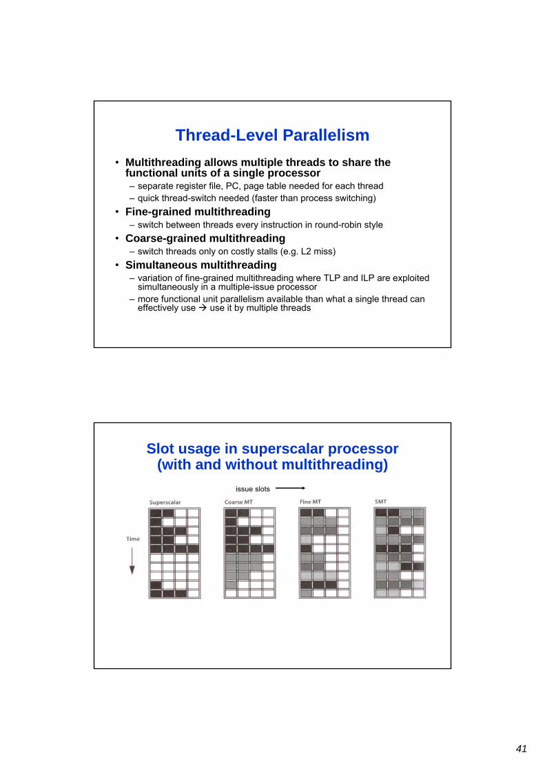
Thread-Level Parallelism• Multithreading allows multiple threads to share the

functional units of a single processor– separate register file, PC, page table needed for each thread– quick thread-switch needed (faster than process switching)

• Fine-grained multithreading– switch between threads every instruction in round-robin style

• Coarse-grained multithreading– switch threads only on costly stalls (e.g. L2 miss)

• Simultaneous multithreading– variation of fine-grained multithreading where TLP and ILP are exploited

simultaneously in a multiple-issue processor– more functional unit parallelism available than what a single thread can

effectively use use it by multiple threads

Slot usage in superscalar processor(with and without multithreading)

issue slots

42

Network design parametersLarge network design space:• topology, degree• routing algorithm

– path, path control, collision resolvement, network support, deadlock handling, livelock handling

• virtual layer support• flow control• buffering• QoS guarantees• error handling• etc, etc.

Circuit-switching and packet-switching

• Circuit-switching– A connection has to be established between the communicating parties

before the transfer can start– The line is reserved for the whole time independently of the amount of

traffic (like the phone line is reserved whether you are silent or talk at your maximum rate)

– The connection will be explicitly closed when there is no more need for the communication

• Packet-switching– The data is packed to carry also information about the destination

address (like a letter or packet in mail)– Separate packets or sub-packets (flits or phits) can be sent along

different routes (if the networks allows that)– Also other senders can inject packets to the network to travel along

(partially) the same route

43

Network Topology• Switched media have a topology that indicate

how nodes are connected• Topology determines

– Degree: number of links from a node– Diameter: max number of links crossed between nodes– Average distance: number of links to random destination– Bisection: minimum number of links that separate the

network into two halves– Bisection bandwidth: link bandwidth x bisection

Network topologies - Mesh• Two-dimensional mesh – very intuitive, indeed

resources

nodes

links

44

Network topologies - Torus• Torus and folded torus extend from mesh

– folded torus has 2x length of the links compared to mesh!

Network topologies - Ring• Ring is the simplest of the networks

– Unidirectional or bidirectional– Does not correspond to the physical placement of resources!

45

Network topologies – Octacon and Spidercon

• Extend the ring by introducing shortcuts– Octacon 4 diagonals– Spidercon N diagonals

Network performance

• Throughput– throughput/input– aggregate throughput– bisection throughput

• Latency– time from data injection to readout

completion

• Inter-related and function of network loading!

020406080

100120140160

10 30 50 70 90

Load %

Throughput

Latency

46

xPipes architecture example –pipelined links

N pipeline stages

N pipeline stages

Part of M cycles for ACK/NACK generation

Part of M cycles forACK/NACK receipt

Source: Davide Bertozzi

Two virtual channels

Example of PROTEO network

47

NOSTRUM basic principle

Source: Axel Jantsch

University of Twente circuit-switched NoC router

CB_SEL

IN

OUT

PORT (HOME)

• Fully connected crossbar• (tri-states or multiplexers)

• Data converter for data• (de-)serializing

• Crossbar configuration memory of 20x5 bit

• Bi-directional links of 2 times • 4 lanes

• Best effort via a separate network

48

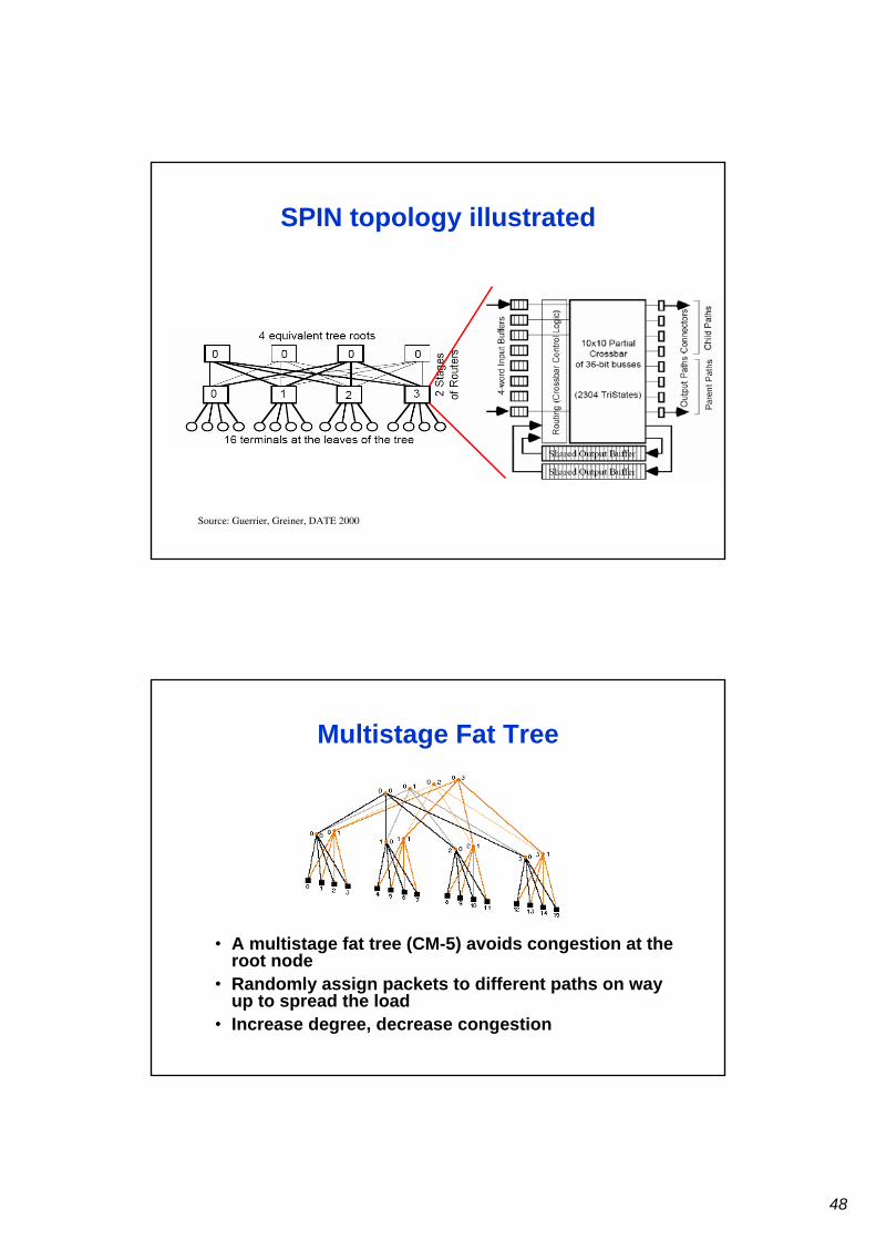
SPIN topology illustrated

Source: Guerrier, Greiner, DATE 2000

Multistage Fat Tree

• A multistage fat tree (CM-5) avoids congestion at the root node

• Randomly assign packets to different paths on way up to spread the load

• Increase degree, decrease congestion

49

Example of XGFT

• Height

• # of child links

• # of parent links

Æthereal distributed GS-BE programming architecture

Source: Goossens et al, D&T of Computers, 2005.

50

Fundamental MP design decisions

• Homogeneous versus Heterogeneous ?• Bus versus Network (and what properties) ?• Shared memory versus Message passing ?• QoS support, Guarantees built-in ?• Generic versus Application specific ?• What types of parallelism to support ?• Focus on Performance, Power or Cost ?• Memory organisation ?

Reliability and availability• A disk subsystem has the following components and

MTTF– 10 disks, each 1,000,000 hours MTTF– 1 SCSI controller, 500,000-hour MTTF– 1 power supply, 200,000-hour MTTF– 1 fan, 200,000-hour MTTF– 1 SCSI cable, 1,000,000 MTTF

• Assuming independent failures, the MTTF for the system is– Failure rate 10 x 1/1M + 1/500,000 + 1/200,000 + 1/200,000 + 1/1M =

23/1M– MTTF = 1/Failure rate = 1M/23 = 43,500 hours (< 5 years)

• Assuming that the system will be serviced within 24 hours of the failure the availability is 43,500/43,524 = 99.94%

• Advertised ”five nines” availability (99.999%) of some computers would mean 5 minute down-time per year!