16.810 16.810

Engineering Design and Rapid PrototypingEngineering Design and Rapid Prototyping

Instructor(s)

Computer Aided Design (CAD)

January 16, 2007

Prof. Olivier de Weck

Lecture 3a

16.810 2

Plan for TodayCAD Lecture (ca. 50 min)

CAD History, BackgroundSome theory on geometrical representation

FEM Lecture (ca. 50 min)Motivation for Structural AnalysisFEM Background

BreakStart creating your own CAD models (ca. 2 hrs)

Work in teams of twoFollow “User Manual” step-by-step, sample partThen start on your own team projectsUse hand sketch (deliverable B) as starting point

16.810 3

Course Concepttodaylast time

16.810 4

Course Flow Diagram (2007)

CAD Introduction

FEM/Solid Mechanics

Avionics Prototyping

CAM Manufacturing

Hand sketching

Initial CAD design

FEM analysis

Optimization

Revise CAD design

Assembly

Parts Fabrication

Problem statement

Final Review

Test

Learning/Review Deliverables(A) Requirements

and Interface Document

(B) Hand Sketch

(D) Manufacturing and Test Report

with Cost Estimate

(C) Solidworks CAD Model, Performance

Analysis

Design Intro / Sketch

Fabrication, Assembly, Testing

(E) CDR Package+ Guest Lectures

16.810 5

What is CAD?

Computer Aided Design (CAD)A set of methods and tools to assist product designers in

Creating a geometrical representation of the artifacts they are designingDimensioning, TolerancingConfiguration Management (Changes)ArchivingExchanging part and assembly information between teams, organizationsFeeding subsequent design steps

Analysis (CAE)Manufacturing (CAM)

…by means of a computer system.

16.810 6

Basic Elements of a CAD SystemInput Devices

Human Designer

ComputerCAD Software

Database

Output Devices

Hard DiskNetworkPrinterPlotter

KeyboardMouse

CAD keyboardTemplatesSpace Ball

Ref: menzelus.com

Main System

16.810 7

Brief History of CAD1957 PRONTO (Dr. Hanratty) – first commercial numerical-control programming system1960 SKETCHPAD (MIT Lincoln Labs)Early 1960’s industrial developments

General Motors – DAC (Design Automated by Computer)McDonnell Douglas – CADD

Early technological developmentsVector-display technologyLight-pens for inputPatterns of lines rendering (first 2D only)

1967 Dr. Jason R Lemon founds SDRC in Cincinnati 1979 Boeing, General Electric and NIST develop IGES (Initial Graphic Exchange Standards), e.g. for transfer of NURBS curvesSince 1981: numerous commercial programs

Source: http://mbinfo.mbdesign.net/CAD-History.htm

16.810 8

Major Benefits of CADProductivity (=Speed) Increase

Automation of repeated tasksDoesn’t necessarily increase creativity!

Insert standard parts (e.g. fasteners) from databaseSupports Changeability

Don’t have to redo entire drawing with each changeEO – “Engineering Orders”

Keep track of previous design iterationsCommunication

With other teams/engineers, e.g. manufacturing, suppliersWith other applications (CAE/FEM, CAM)Marketing, realistic product renderingAccurate, high quality drawings

Caution: CAD Systems produce errors with hidden lines etc…

Some limited AnalysisMass Properties (Mass, Inertia)Collisions between parts, clearances

16.810 9

Generic CAD ProcessStart

Settings Units, Grid (snap), …

Construct Basic Solids

Boolean Operations(add, subtract, …)

AnnotationsDimensioning

Verification

Create lines, radii, partcontours, chamfers

Add cutouts & holes

Engineering Sketch

dim3D 2D

extrude, rotate

CAD file

Drawing (dxf)

IGES fileOutput

-

=

x.x

16.810 10

Boeing (sample) partsA/C structural assembly

2 decks3 framesKeel

Loft included to show interface/stayout zone to A/CAll Boeing parts in Catiafile format

Files imported into SolidWorks by converting to IGES format

Loft

FWD Decks

Aft Decks

Frames

Keel

(Loft not shown)

Example CAD A/C Assembly

Nacelle

16.810 11

Vector versus Raster GraphicsRaster Graphics

Grid of pixelsNo relationships between pixelsResolution, e.g. 72 dpi (dots per inch)Each pixel has color, e.g. 8-bit image has 256 colors

.bmp - raw data format

16.810 12

Vector Graphics

Object Orientedrelationship between pixels captureddescribes both (anchor/control) points and lines between themEasier scaling & editing

.emf format

CAD Systems usevector graphics

Most common interface file:IGES

16.810 13

Major CAD Software Products

AutoCAD (Autodesk) mainly for PCPro Engineer (PTC)SolidWorks (Dassault Systems)CATIA (IBM/Dassault Systems)Unigraphics (UGS)I-DEAS (SDRC)

16.810 14

Some CAD-Theory

(1) Parametric Curve Equation vs.

Nonparametric Curve Equation

(2) Various curves (some mathematics !)

- Hermite Curve

- Bezier Curve

- B-Spline Curve

- NURBS (Nonuniform Rational B-Spline) Curves

Applications: CAD, FEM, Design Optimization

Geometrical representation

16.810 15

Curve EquationsTwo types of equations for curve representation

(1) Parametric equation

x, y, z coordinates are related by a parametric variable

(2) Nonparametric equation

x, y, z coordinates are related by a function

Parametric equation

cos , sin (0 2 )x R y Rθ θ θ π= = ≤ ≤

Example: Circle (2-D)

Nonparametric equation2 2 2 0x y R+ − =

2 2y R x= ± −

(Implicit nonparametric form)

(Explicit nonparametric form)

( or )u θ

16.810 16

Curve EquationsTwo types of curve equations

(1) Parametric equation

( ) : 2-D , ( , ) : 3-Dy f x z f x y= =(2) Nonparametric equation

Point on 2-D curve: [ ( ) ( )]x u y u=p

Point on 3-D surface: [ ( ) ( ) ( )]x u y u z u=p

: parametric variable and independent variableu

Which is better for CAD/CAE? : Parametric equation

cos , sin (0 2 )x R y Rθ θ θ π= = ≤ ≤

2 2 2 0x y R+ − =

2 2y R x= ± −

θΔ

It also is good for calculating the points at a certain interval along a curve

16.810 17

Parametric Equations –Advantages over nonparametric forms

1. Parametric equations usually offer more degrees of freedom for controlling the shape of curves and surfaces than do nonparametric forms.

e.g. Cubic curve

3 2Nonparametric curve: y ax bx cx d= + + +

3 2

3 2

Parametric curve:

x au bu cu dy eu fu gx h= + + +

= + + +

3. Transformation can be performed directly on parametric equationse.g. Translation in x-dir.

3 20 0 0Nonparametric curve: ( ) ( ) ( )y a x x b x x c x x d= − + − + − +

3 20

3 2

Parametric curve:

x au bu cu d x

y eu fu gx h

= + + + +

= + + +

//

dy dy dudx dx du

= ⇒

2. Parametric forms readily handle infinite slopes

/ 0 indicates /dx du dy dx= = ∞

16.810 18

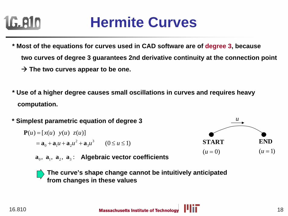
Hermite Curves* Most of the equations for curves used in CAD software are of degree 3, because

two curves of degree 3 guarantees 2nd derivative continuity at the connection point

The two curves appear to be one.

* Use of a higher degree causes small oscillations in curves and requires heavy

computation.

2 30 1 2 3

( ) [ ( ) ( ) ( )](0 1)

u x u y u z uu u u u

=

= + + + ≤ ≤

Pa a a a

* Simplest parametric equation of degree 3

0 1 2 3, , , :a a a a Algebraic vector coefficients

The curve’s shape change cannot be intuitively anticipated from changes in these values

u

( 0)u =START

( 1)u =END

16.810 19

Hermite Curves2 3

0 1 2 3( ) (0 1)u u u u u= + + + ≤ ≤P a a a a

Instead of algebraic coefficients, let’s use the position vectors and the tangent vectors at the two end points!

0P1P

( 0)u =START

( 1)u =END

0′P

1′P

u0 0

1 0 1 2 3

0 1

1 1 2

Position vector at starting point: (0)Position vector at end point: (1)

Tangent vector at starting point: (0)

Tangent vector at end point: (1) 2 3

= == = + + +

′ ′= =

′ ′= = + +

P P aP P a a a a

P P a

P P a a 3a

No algebraic coefficients

0 0 1 1, , , :′ ′P P P P Geometric coefficients

The curve’s shape change can be intuitively anticipated from changes in these values

0

12 3 2 3 2 3 2 3

0

1

( ) [1 3 2 3 2 2 ]u u u u u u u u u u

⎡ ⎤⎢ ⎥⎢ ⎥

= − + − − + − + ⎢ ⎥′⎢ ⎥⎢ ⎥′⎣ ⎦

PP

PP

P

Blending functions

: Hermit curve

16.810 20

u(1,1)( 0)u =START (5,1)

( 1)u =END

0

1

0

1

(0)(1)

: Geometric coefficient matrix(0)

(1)

⎡ ⎤ ⎡ ⎤⎢ ⎥ ⎢ ⎥⎢ ⎥ ⎢ ⎥=⎢ ⎥ ⎢ ⎥′ ′⎢ ⎥ ⎢ ⎥⎢ ⎥ ⎢ ⎥′ ′⎣ ⎦⎣ ⎦

P PP P

P P

PP

Effect of tangent vectors on the curve’s shape

⎡ ⎤⎢ ⎥⎢ ⎥⎢ ⎥⎢ ⎥⎣ ⎦

1 15 11 11 -1

⎡ ⎤⎢ ⎥⎢ ⎥⎢ ⎥⎢ ⎥⎣ ⎦

1 15 15 55 -5

⎡ ⎤⎢ ⎥⎢ ⎥⎢ ⎥⎢ ⎥⎣ ⎦

1 15 113 1313 -13

Is this what you really wanted?

⎡ ⎤⎢ ⎥⎢ ⎥⎢ ⎥⎢ ⎥⎣ ⎦

1 15 12 22 -2

Geometric coefficient matrix controls the shape of the curve

⎡ ⎤⎢ ⎥⎢ ⎥⎢ ⎥⎢ ⎥⎣ ⎦

1 15 14 04 0

/ 0 0/ 4

dy dy dudx dx du

= = =

16.810 21

Bezier Curve* In case of Hermite curve, it is not easy to predict curve shape caused by changes in the magnitude of the tangent vectors,0 1 and ′ ′P P

0

!( ) (1 ) , where!( )!

ni n i

ii

n n nu u ui i i n i

−

=

⎛ ⎞ ⎛ ⎞= − =⎜ ⎟ ⎜ ⎟ −⎝ ⎠ ⎝ ⎠∑P P

:iP Position vector of the i th vertex (control vertices)

* Bezier Curve can control curve shape more easily using several control points (Bezier 1960)

Control vertices

Control polygonn=3

0P

1P 2P

3P * Order of the curve: n

* Number of vertices: n+1(No of control points)

* Number of segments: n

* The order of Bezier curve is determined by the number of control points.

n control points Order of Bezier curve: n-1

16.810 22

Bezier Curve

- The curve passes through the first and last vertex of the polygon.

-The tangent vector at the starting point of the curve has the same direction as the first segment of the polygon.

- The nth derivative of the curve at the starting or ending point is determined by the first or last (n+1) vertices.

Properties

16.810 23

(1) For complicated shape representation, higher degree Bezier curves are

needed.

Oscillation in curve occurs, and computational burden increases.

Two Drawbacks of Bezier curve

(2) Any one control point of the curve affects the shape of the entire curve.

Modifying the shape of a curve locally is difficult.

(Global modification property)

Desirable properties :

1. Ability to represent complicated shape with low order of the curve

2. Ability to modify a curve’s shape locally

B-spline curve!

16.810 24

B-Spline Curve

,0

, 1 1, 1,

1 1

1,1

( ) ( )

where: Position vector of the th control point

( ) ( ) ( ) ( )( )

1( )

0 otherwise

n

i k ii

i

i i k i k i ki k

i k i i k i

i ii

u N u

iu t N u t u N u

N ut t t t

t u tN u

=

− + + −

+ − + +

+

=

− −= +

− −

≤ ≤⎧= ⎨⎩

∑P P

P

k: order of the B-spline curve

n+1: number of control points

0 012

i

i kt i k k i n

n k n i n k

≤ <⎧⎪= − + ≤ ≤⎨⎪ − + < ≤ +⎩(Nonperiodic knots)

* Developed by Cox and Boor (1972)

The order of curve is independent of the number of control points!

16.810 25

B-Spline Curve

Example

Order (k) = 3 (first derivatives are continuous)

No of control points (n+1) = 6

(1) The order of the curve is independent of the number of control points (contrary to Bezier curves)

- User can select the curve’s order and number of control points separately.

- It can represent very complicated shape with low order

(2) Modifying the shape of a curve locally is easy. (contrary to Bezier curve)

- Each curve segment is affected by k (order) control points. (local modification property)

Advantages

16.810 26

NURBS (Nonuniform Rational B-Spline) Curve

,0

,0

( )( )

( )

n

i i i ki

n

i i ki

h N uu

h N u

=

=

=∑

∑

PP ,

0B-spline : ( ) ( )

n

i i ki

u N u=

⎛ ⎞=⎜ ⎟⎝ ⎠

∑P P

: Position vector of the th control point: Homogeneous coordinate

i

i

ihP

* If all the homogeneous coordinates (hi) are 1, the denominator becomes 1

,0

If 0 , then ( ) 1.n

i i i ki

h i h N u=

= ∀ =∑

* B-spline curve is a special case of NURBS.

* Bezier curve is a special case of B-spline curve.

16.810 27

Advantages of NURBS Curve over B-Spline Curve

(1) More versatile modification capacity

- Homogeneous coordinate hi, which B-spline does not have, can change.

- Increasing hi of a control point Drawing the curve toward the control point.

(2) NURBS can exactly represent the conic curves - circles, ellipses, parabolas, and

hyperbolas (B-spline can only approximate these curves)

(3) Curves, such as conic curves, Bezier curves, and B-spline curves can be

converted to their corresponding NURBS representations.

16.810 28

(1) Parametric Equation vs. Nonparametric Equation

(2) Various curves

- Hermite Curve

- Bezier Curve

- B-Spline Curve

- NURBS (Nonuniform Rational B-Spline) Curve

(3) Surfaces

- Bilinear surface

- Bicubic surface

- Bezier surface

- B-Spline surface

- NURBS surface

Summary

16.810 29

SolidWorks

SolidWorksMost popular CAD system in educationWill be used for this projectDo Self-Introduction via 16.810 User ManualSee also

http://www.solidworks.com (Student Section)