Computer-Aided Circuit Simulation and Verification

CSE245 – Fall 2004Professor:Chung-Kuan Cheng

Administration• Lectures: 5:00pm ~ 6:20pm TTH HSS 2152• Office Hours: 4:00pm ~ 4:45pm TTH APM 4256• Textbook

Electronic Circuit and System Simulation MethodsT.L. Pillage, R.A. Rohrer, C. Visweswariah, McGraw-Hill

• TA: Zhengyong (Simon) Zhu (zzhu@cs.ucsd.edu)

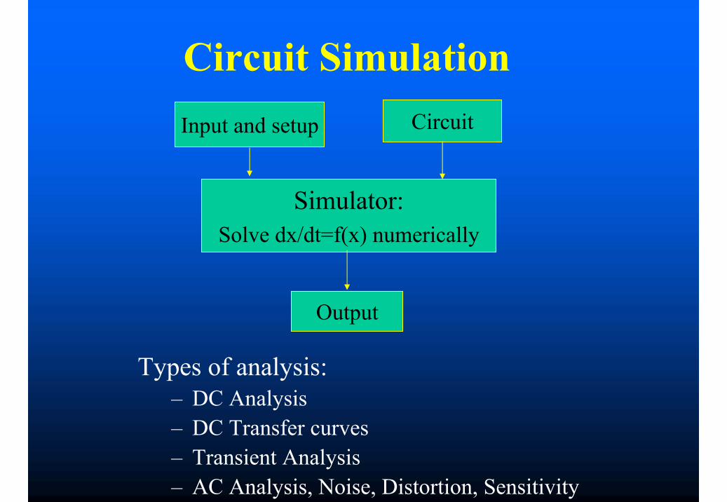
Circuit Simulation

Simulator:Solve dx/dt=f(x) numerically

Input and setup Circuit

Output

Types of analysis:– DC Analysis– DC Transfer curves– Transient Analysis– AC Analysis, Noise, Distortion, Sensitivity

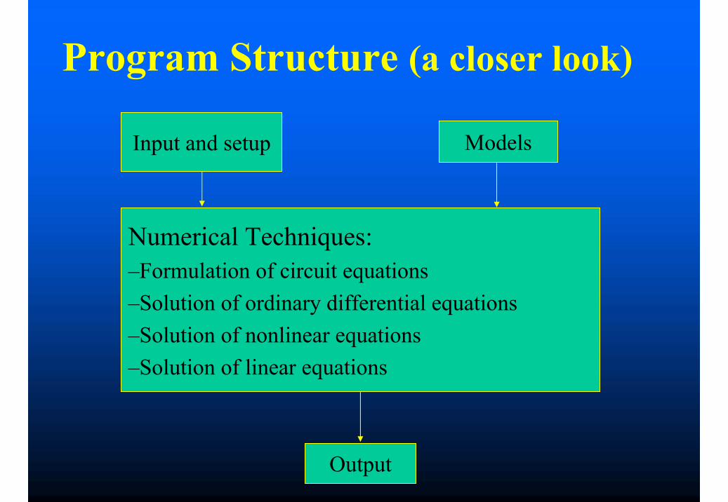
Program Structure (a closer look)

Numerical Techniques:–Formulation of circuit equations –Solution of ordinary differential equations–Solution of nonlinear equations–Solution of linear equations

Input and setup Models

Output

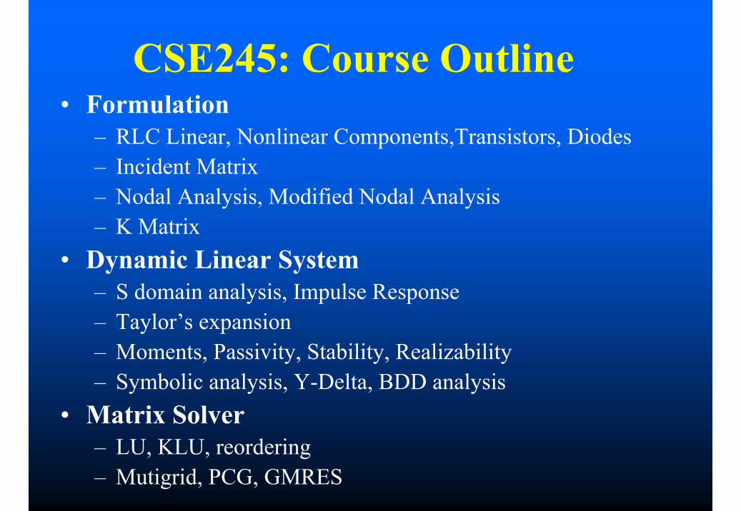
CSE245: Course Outline• Formulation

– RLC Linear, Nonlinear Components,Transistors, Diodes– Incident Matrix– Nodal Analysis, Modified Nodal Analysis– K Matrix

• Dynamic Linear System– S domain analysis, Impulse Response – Taylor’s expansion– Moments, Passivity, Stability, Realizability– Symbolic analysis, Y-Delta, BDD analysis

• Matrix Solver – LU, KLU, reordering– Mutigrid, PCG, GMRES

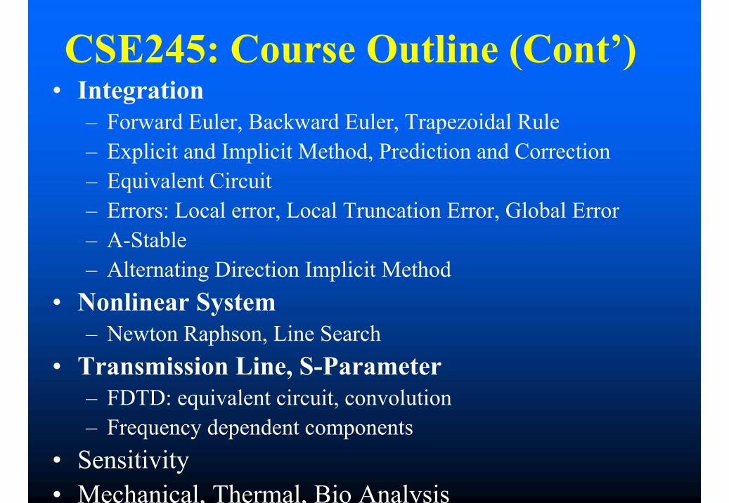
CSE245: Course Outline (Cont’)• Integration

– Forward Euler, Backward Euler, Trapezoidal Rule– Explicit and Implicit Method, Prediction and Correction– Equivalent Circuit– Errors: Local error, Local Truncation Error, Global Error– A-Stable– Alternating Direction Implicit Method

• Nonlinear System– Newton Raphson, Line Search

• Transmission Line, S-Parameter– FDTD: equivalent circuit, convolution– Frequency dependent components

• Sensitivity• Mechanical, Thermal, Bio Analysis

Lecture 1: Formulation

• KCL/KVL• Sparse Tableau Analysis• Nodal Analysis, Modified Nodal Analysis

*some slides borrowed from Berkeley EE219 Course

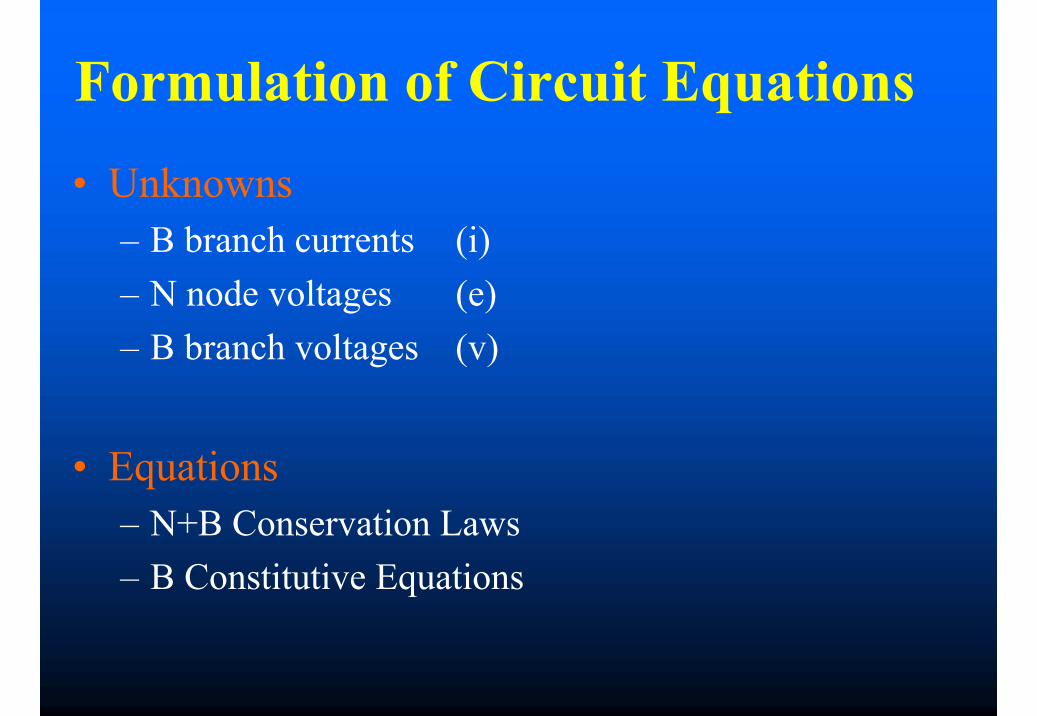
Formulation of Circuit Equations

• Unknowns– B branch currents (i)– N node voltages (e)– B branch voltages (v)

• Equations– N+B Conservation Laws – B Constitutive Equations

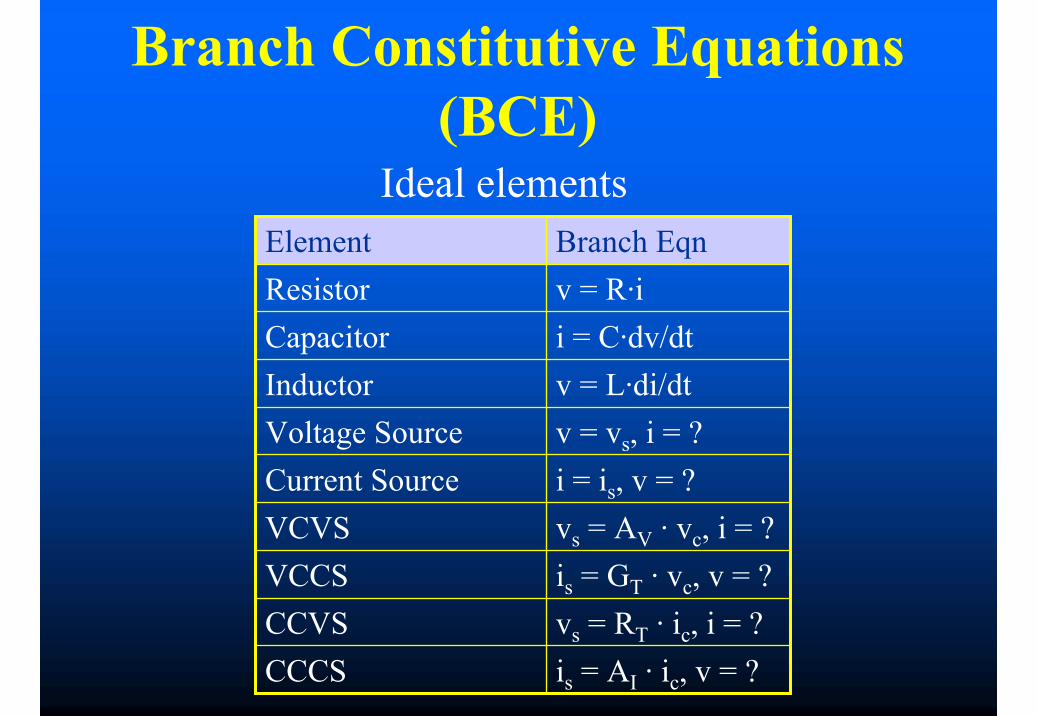
Branch Constitutive Equations (BCE)

Ideal elements

is = AI · ic, v = ?CCCSvs = RT · ic, i = ?CCVSis = GT · vc, v = ?VCCSvs = AV · vc, i = ?VCVSi = is, v = ?Current Sourcev = vs, i = ?Voltage Sourcev = L·di/dtInductori = C·dv/dtCapacitorv = R·iResistorBranch EqnElement

Conservation Laws

• Determined by the topology of the circuit• Kirchhoff’s Voltage Law (KVL): Every circuit

node has a unique voltage with respect to the reference node. The voltage across a branch eb is equal to the difference between the positive and negative referenced voltages of the nodes on which it is incident– No voltage source loop

• Kirchhoff’s Current Law (KCL): The algebraic sum of all the currents flowing out of (or into) any circuit node iszero.– No Current Source Cut

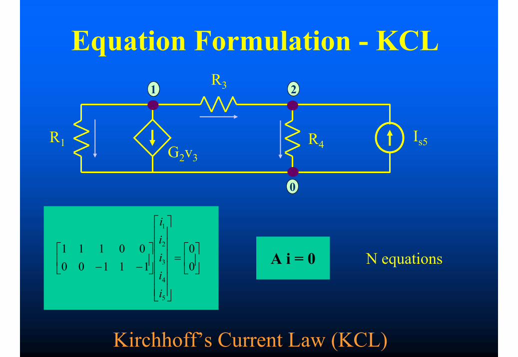
Equation Formulation - KCL

0

1 2

R1G2v3

R3

R4 Is5

=

−− 0

011100

00111

5

4

3

2

1

iiiii

A i = 0

Kirchhoff’s Current Law (KCL)

N equations

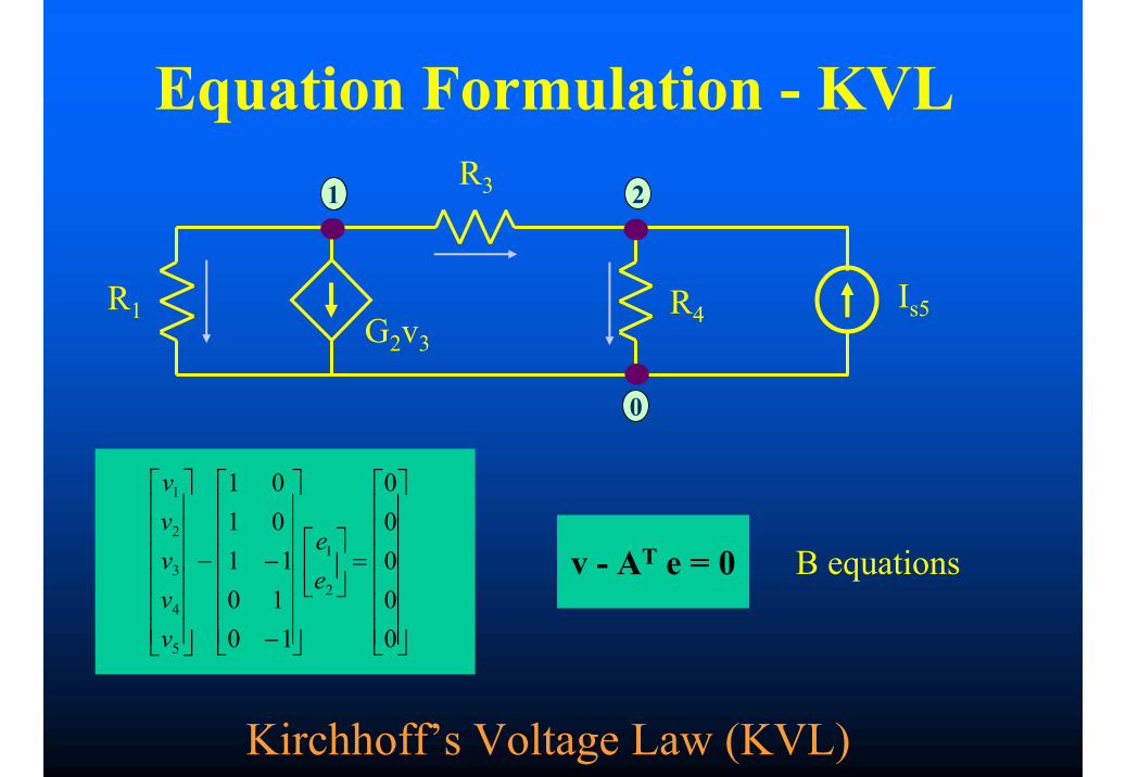
Equation Formulation - KVL

0

1 2

R1G2v3

R3

R4 Is5

=

−

−−

00000

101011

0101

2

1

5

4

3

2

1

ee

vvvvv

v - AT e = 0

Kirchhoff’s Voltage Law (KVL)

B equations

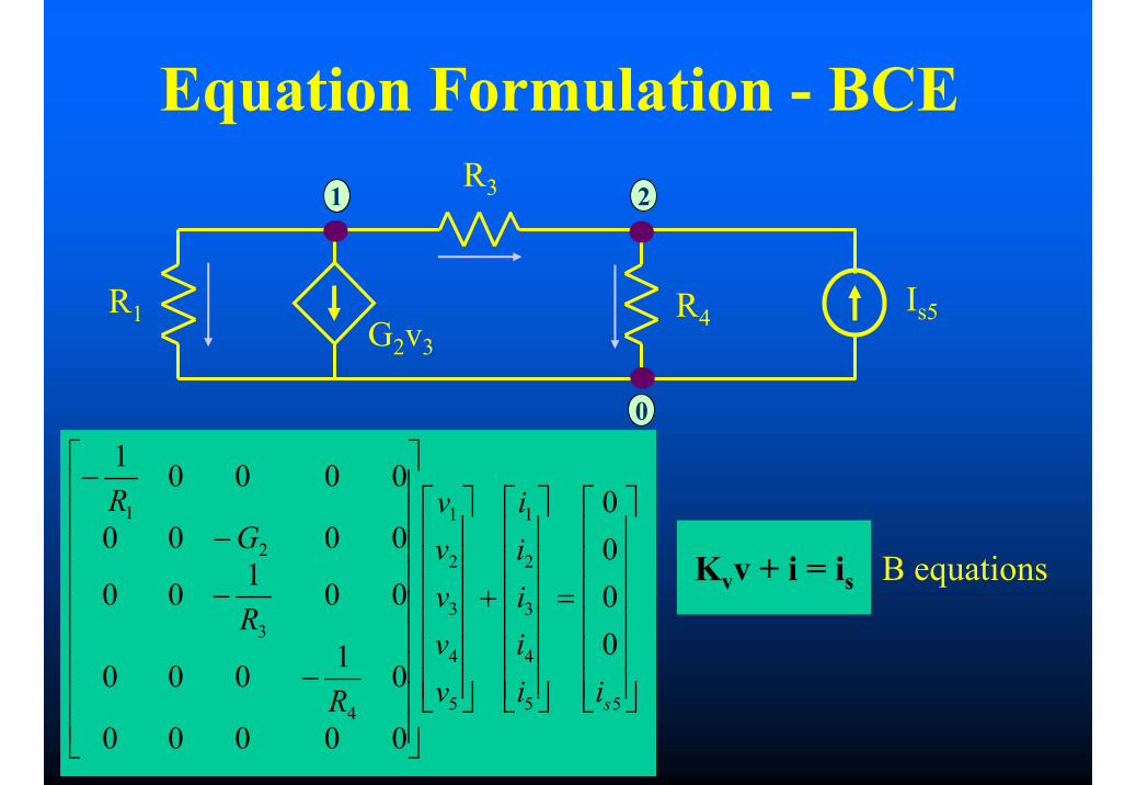
Equation Formulation - BCE

0

1 2

R1G2v3

R3

R4 Is5

=

+

−

−

−

−

55

4

3

2

1

5

4

3

2

1

4

3

2

1

0000

00000

01000

00100

0000

00001

siiiiii

vvvvv

R

R

GR

Kvv + i = is B equations

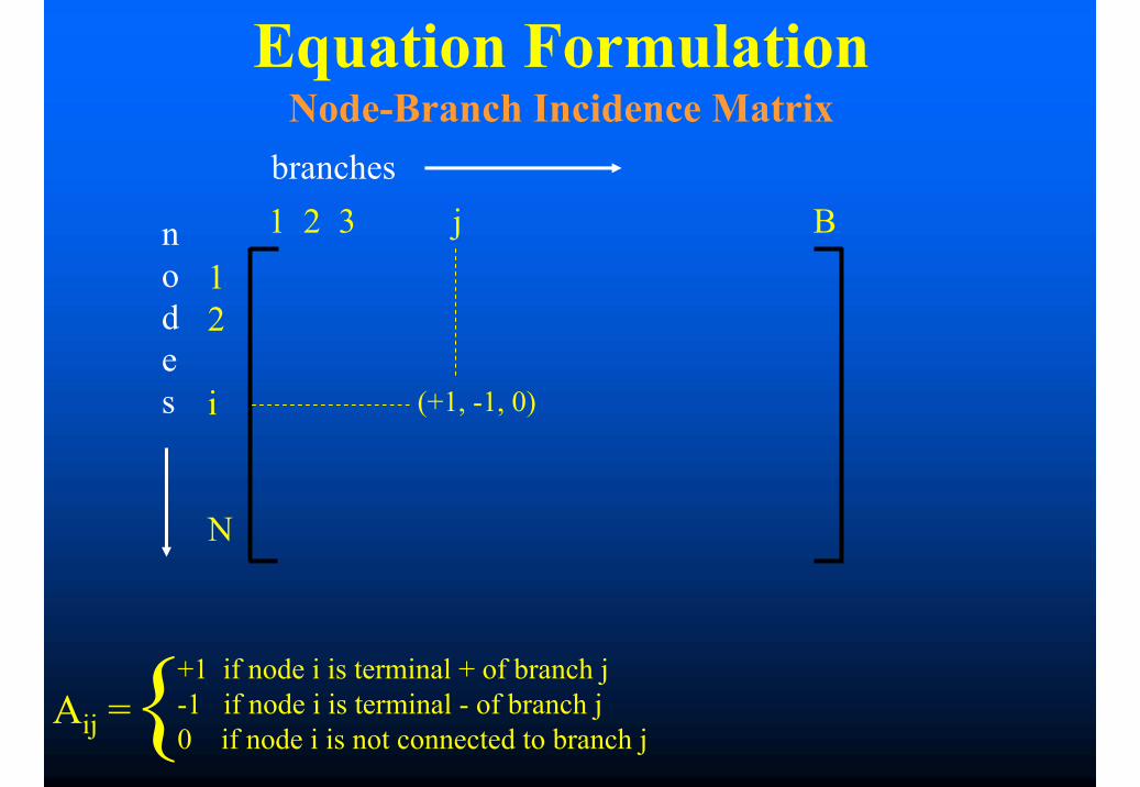
Equation FormulationNode-Branch Incidence Matrix

1 2 3 j B12

i

N

branches

nodes (+1, -1, 0)

{Aij =+1 if node i is terminal + of branch j-1 if node i is terminal - of branch j0 if node i is not connected to branch j

Equation Assembly (Stamping Procedures)

• Different ways of combining Conservation Laws and Constitutive Equations– Sparse Table Analysis (STA)– Modified Nodal Analysis (MNA)

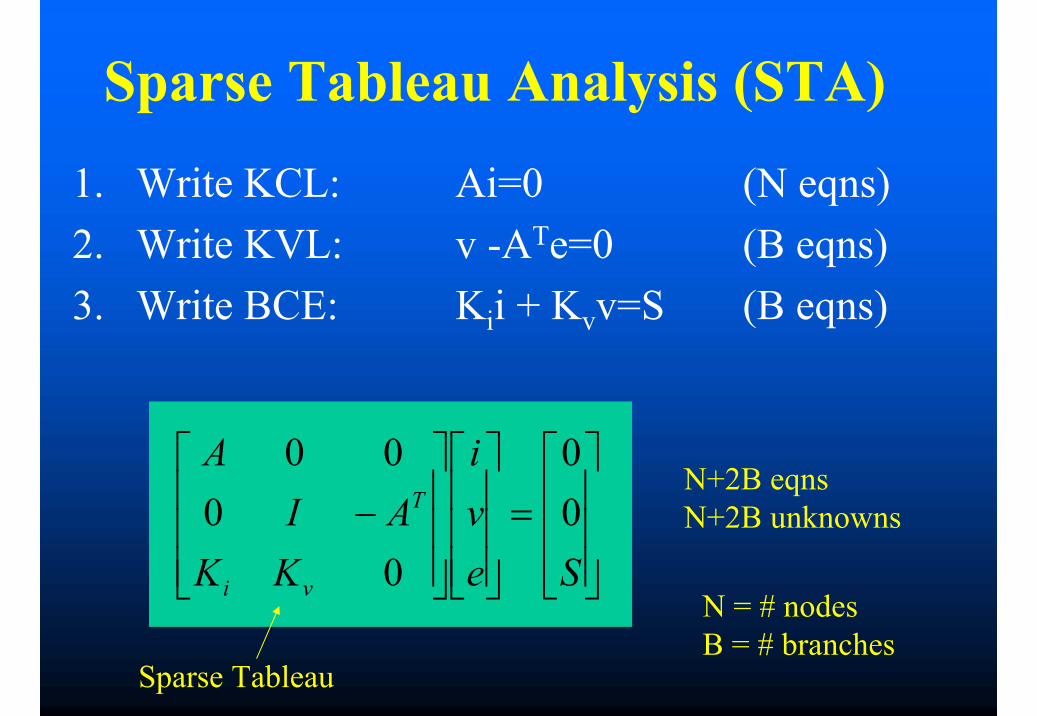
Sparse Tableau Analysis (STA)

1. Write KCL: Ai=0 (N eqns)2. Write KVL: v -ATe=0 (B eqns)3. Write BCE: Kii + Kvv=S (B eqns)

=

−

Sevi

KKAI

A

vi

T 00

00

00N+2B eqnsN+2B unknowns

N = # nodesB = # branches

Sparse Tableau

Sparse Tableau Analysis (STA)Advantages• It can be applied to any circuit• Eqns can be assembled directly from input data• Coefficient Matrix is very sparse

ProblemSophisticated programming techniques and datastructures are required for time and memoryefficiency

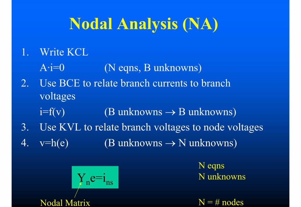
Nodal Analysis (NA)1. Write KCL

A·i=0 (N eqns, B unknowns)2. Use BCE to relate branch currents to branch

voltagesi=f(v) (B unknowns → B unknowns)

3. Use KVL to relate branch voltages to node voltages4. v=h(e) (B unknowns → N unknowns)

Yne=ins

N eqnsN unknowns

N = # nodesNodal Matrix

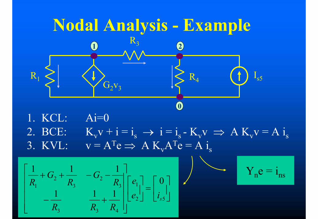
Nodal Analysis - ExampleR3

0

1 2

R1G2v3

R4 Is5

1. KCL: Ai=02. BCE: Kvv + i = is → i = is - Kvv ⇒ A Kvv = A is3. KVL: v = ATe ⇒ A KvATe = A is

Yne = ins

=

+−

−−++

52

1

433

32

32

10

111

111

siee

RRR

RG

RG

R

Nodal Analysis

• Example shows NA may be derived from STA

• Better: Yn may be obtained by direct inspection (stamping procedure)– Each element has an associated stamp– Yn is the composition of all the elements’ stamps

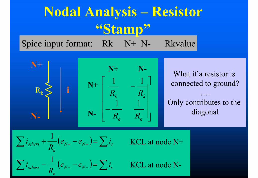
Spice input format: Rk N+ N- Rkvalue

Nodal Analysis – Resistor “Stamp”

−

−

kk

kk

RR

RR11

11N+ N-

N+

N-

N+

N-

iRk

( )

( ) ∑∑

∑∑

=−−

=−+

−+

−+

sNNk

others

sNNk

others

ieeR

i

ieeR

i

1

1KCL at node N+

KCL at node N-

What if a resistor is connected to ground?

….Only contributes to the

diagonal

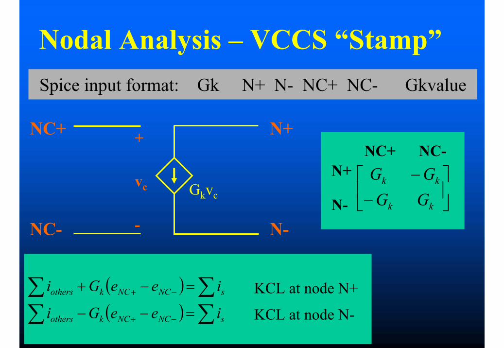
Spice input format: Gk N+ N- NC+ NC- Gkvalue

Nodal Analysis – VCCS “Stamp”

−

−

kk

kk

GGGG

NC+ NC-N+

N-

N+

N-

Gkvc

NC+

NC-

+

vc

-

( )( ) ∑∑

∑∑=−−

=−+

−+

−+

sNCNCkothers

sNCNCkothers

ieeGi

ieeGi KCL at node N+

KCL at node N-

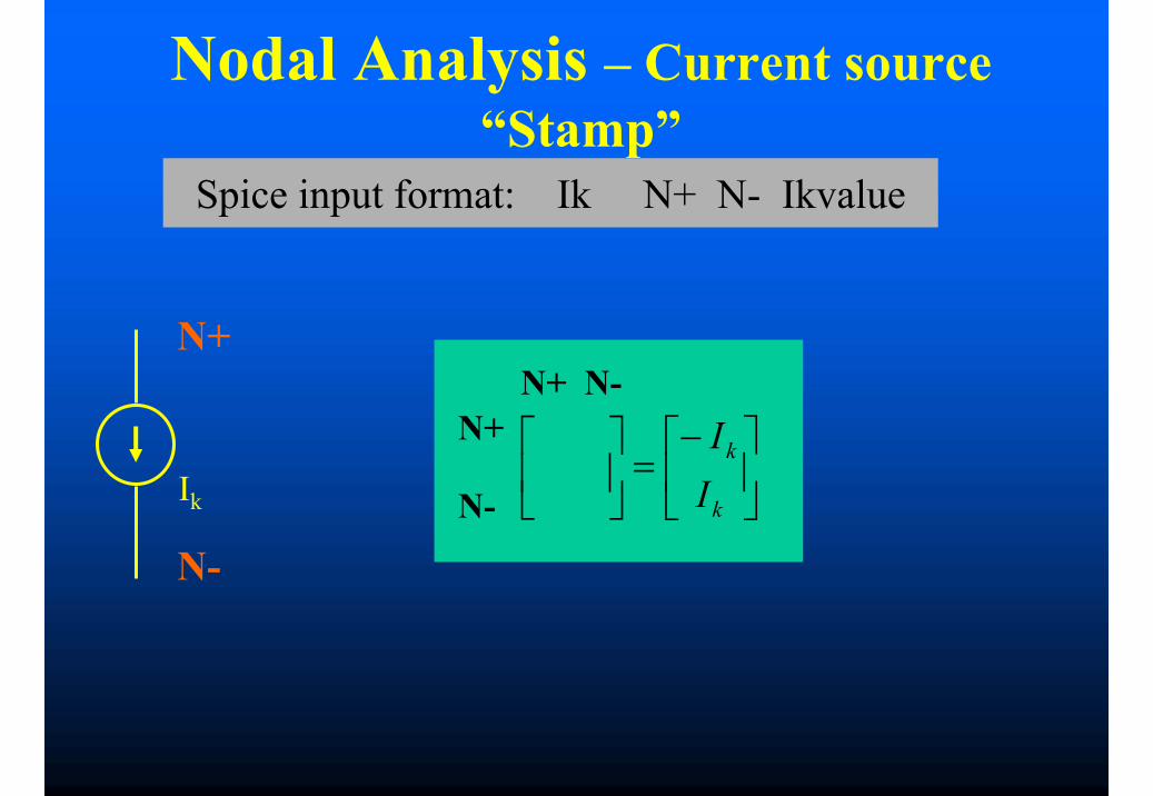
Spice input format: Ik N+ N- Ikvalue

Nodal Analysis – Current source “Stamp”

−=

k

k

II

N+ N-N+

N-

N+

N-

Ik

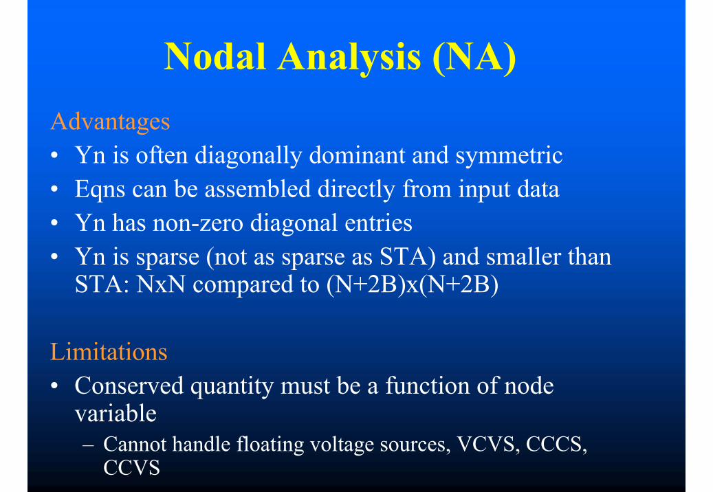
Nodal Analysis (NA)Advantages• Yn is often diagonally dominant and symmetric• Eqns can be assembled directly from input data• Yn has non-zero diagonal entries• Yn is sparse (not as sparse as STA) and smaller than

STA: NxN compared to (N+2B)x(N+2B)

Limitations• Conserved quantity must be a function of node

variable– Cannot handle floating voltage sources, VCVS, CCCS,

CCVS

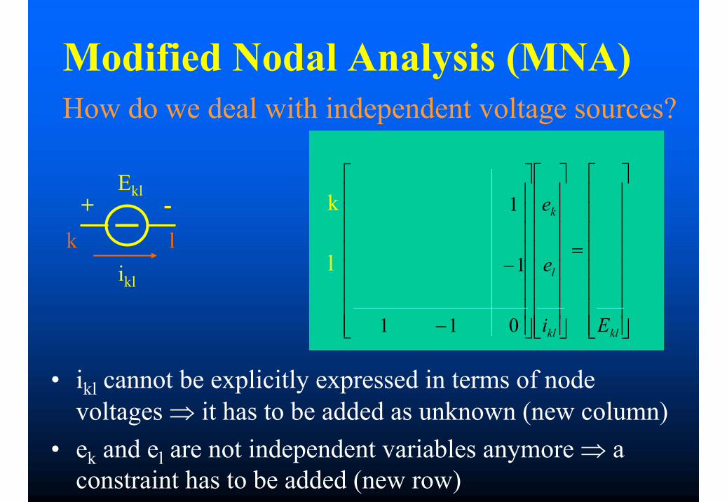
Modified Nodal Analysis (MNA)

• ikl cannot be explicitly expressed in terms of node voltages ⇒ it has to be added as unknown (new column)

• ek and el are not independent variables anymore ⇒ a constraint has to be added (new row)

How do we deal with independent voltage sources?

ikl

k l+ -

Ekl

=

−

−

klkl

l

k

Ei

e

e

011

1

1k

l

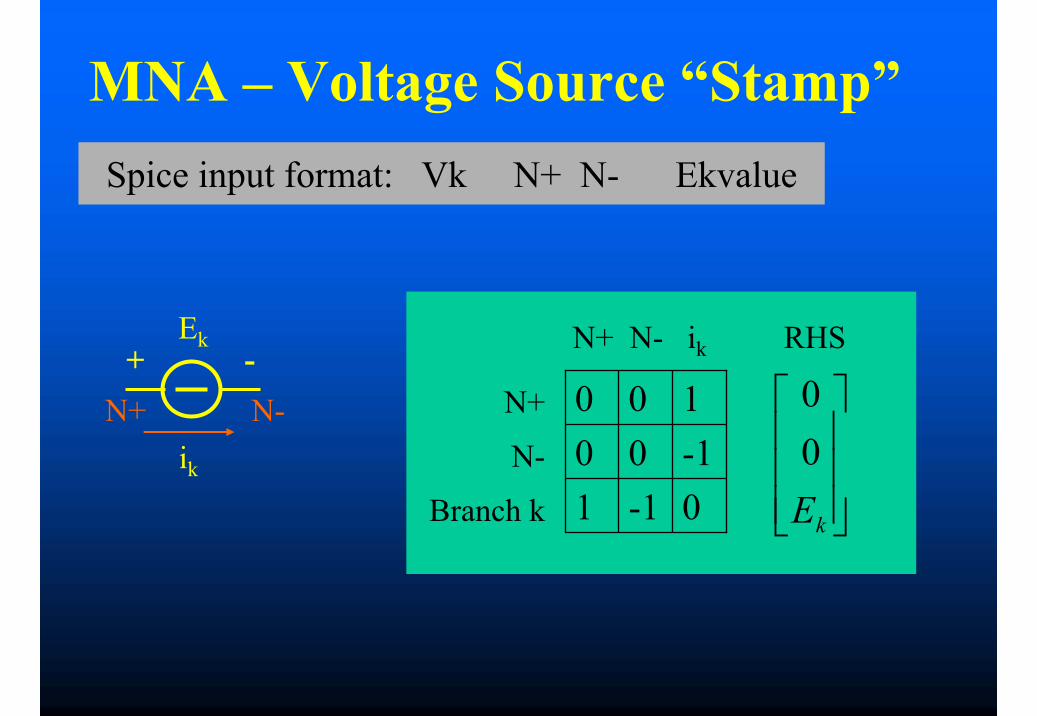
MNA – Voltage Source “Stamp”

ik

N+ N-+ -

Ek

Spice input format: Vk N+ N- Ekvalue

kE00

0-11-100100N+

N-

Branch k

N+ N- ik RHS

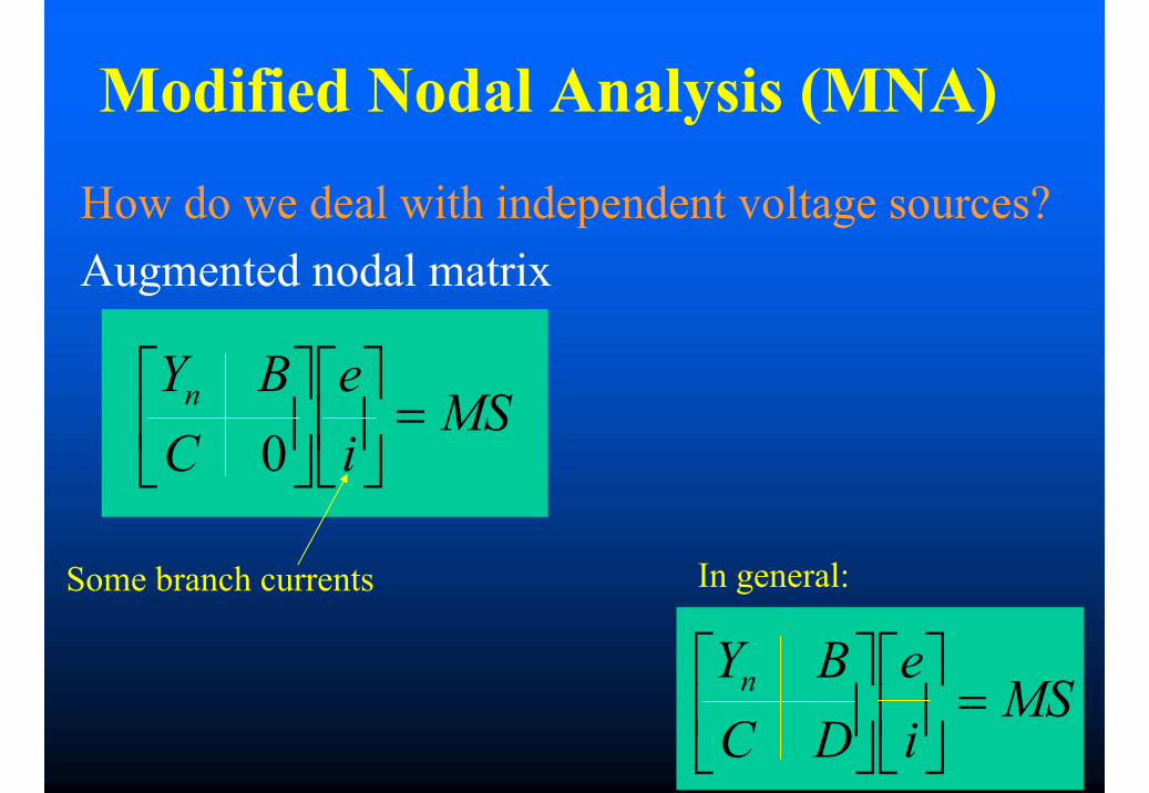
Modified Nodal Analysis (MNA)

How do we deal with independent voltage sources?Augmented nodal matrix

MSie

CBYn =

0

Some branch currents

MSie

DCBYn =

In general:

MNA – General rules

• A branch current is always introduced as and additional variable for a voltage source or an inductor

• For current sources, resistors, conductors and capacitors, the branch current is introduced only if:– Any circuit element depends on that branch current– That branch current is requested as output

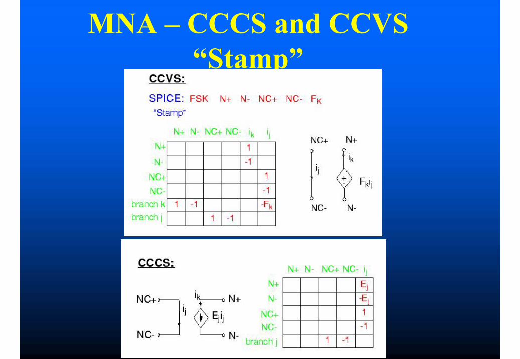
MNA – CCCS and CCVS “Stamp”

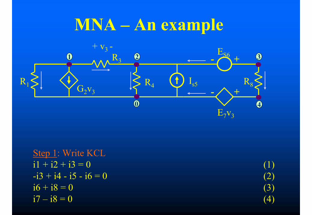
MNA – An example

Step 1: Write KCLi1 + i2 + i3 = 0 (1)-i3 + i4 - i5 - i6 = 0 (2)i6 + i8 = 0 (3)i7 – i8 = 0 (4)

0

1 2

G2v3R4 Is5R1

ES6- +

R8

3

E7v3

- +4

+ v3 -R3

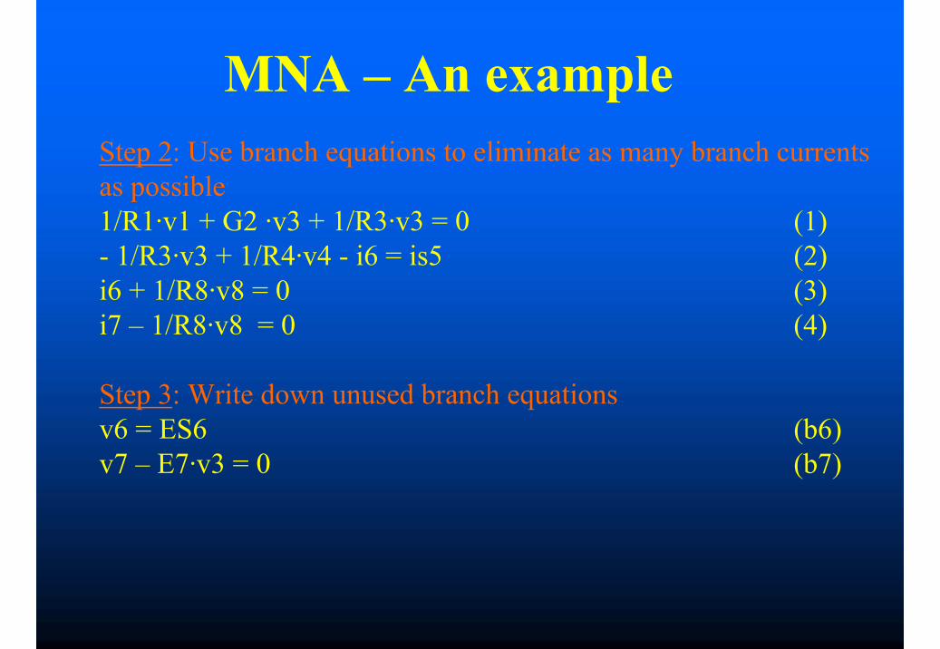
MNA – An exampleStep 2: Use branch equations to eliminate as many branch currents as possible1/R1·v1 + G2 ·v3 + 1/R3·v3 = 0 (1)- 1/R3·v3 + 1/R4·v4 - i6 = is5 (2)i6 + 1/R8·v8 = 0 (3)i7 – 1/R8·v8 = 0 (4)

Step 3: Write down unused branch equationsv6 = ES6 (b6)v7 – E7·v3 = 0 (b7)

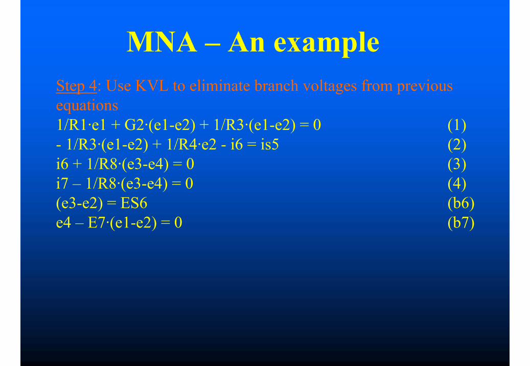
MNA – An exampleStep 4: Use KVL to eliminate branch voltages from previous equations1/R1·e1 + G2·(e1-e2) + 1/R3·(e1-e2) = 0 (1)- 1/R3·(e1-e2) + 1/R4·e2 - i6 = is5 (2)i6 + 1/R8·(e3-e4) = 0 (3)i7 – 1/R8·(e3-e4) = 0 (4)(e3-e2) = ES6 (b6)e4 – E7·(e1-e2) = 0 (b7)

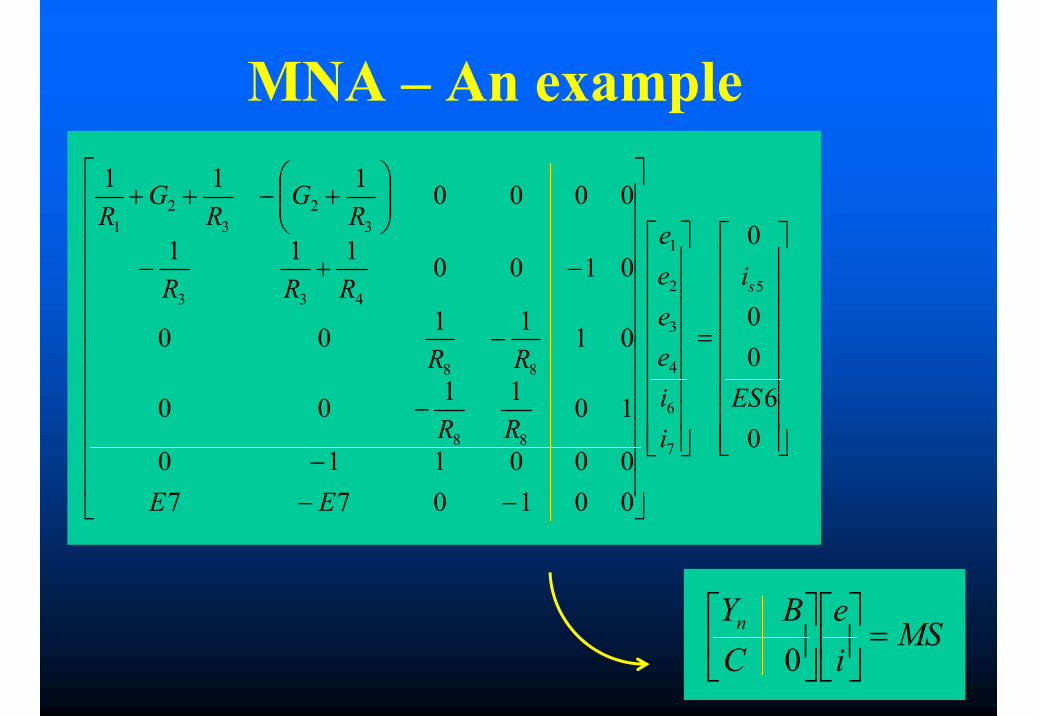
MNA – An example

=

−−−

−

−

−+−

+−++

06

00

0

001077000110

101100

011100

0100111

0000111

5

7

6

4

3

2

1

88

88

433

32

32

1

ES

i

iieeee

EE

RR

RR

RRR

RG

RG

R

s

MSie

CBYn =

0

Modified Nodal Analysis (MNA)

Advantages• MNA can be applied to any circuit• Eqns can be assembled directly from input data• MNA matrix is close to Yn

Limitations• Sometimes we have zeros on the main

diagonal