Compute Unified Device Architecture (CUDA) Based … Terms—FDTD methods, parallel architectures,...

Abstract— Recent developments in the design of graphics processing units (GPUs) have made it possible to use these devices as alternatives to central processor units (CPUs) and perform high performance scientific computing on them. Though several implementations of finite-difference time-domain (FDTD) method have been reported, the unavailability of high level languages to program graphics cards had been a major obstacle for scientists and engineers who would want to develop codes for graphics cards. Relatively recently, compute unified device architecture (CUDA) development environment has been introduced by NVIDIA and made GPU computing much easier. This paper presents an implementation of FDTD method based on CUDA. Two thread-to-cell mapping algorithms are presented. The details of the implementation are provided and strategies to improve the performance of the FDTD simulations are discussed. Index Terms—FDTD methods, parallel architectures, graphics processing unit (GPU) programming, Compute Unified Device Architecture (CUDA), hardware accelerated computing.

I. INTRODUCTION Recent developments in the design of graphics

processing units (GPUs) have been occurring at a much greater pace than with central processor units (CPUs) and very powerful processing units have been designed solely for the processing of

computer graphics. For instance, the current generation of GPU based NVIDIA® Tesla™ C1060 Computing Processors are running at approximately 1.3 GHz with a 512 bit data and memory bandwidth of 102 GB/sec. While GPU clock speed seems slow compared to modern 3.8 GHz Pentium CPU’s or 3.0 GHz Core Duo’s, parallelism provided by the graphics cards enables better efficiency in computations. Due to this potential in faster computations, the GPUs have received the attention of the scientific computing community. Initially these cards were designed for computer graphics and floating precision arithmetic has been sufficient for such applications. Due to the demand of higher precision arithmetic from the scientific community, the vendors have started to develop graphics cards that support double precision arithmetic as well, introducing a new generation of graphical computation cards.

The computational electromagnetics community as well has started to utilize the computational power of graphics cards, and in particular, several implementations of finite-difference time-domain (FDTD) [1]-[3] method have been reported [4]-[24]. Initially the GPUs were not designed for general purpose programming and high level programming languages were not conveniently available; programmers were required to learn the intricacies of specialized low-level hardware languages. For instance, the FDTD implementations in [4], [5] and [11] are based on OpenGL. As a result of the need for high level languages a new subset language for C titled “Brook” has been introduced for general

Veysel Demir1 and Atef Z. Elsherbeni2

1Department of Electrical Engineering Northern Illinois University, DeKalb, IL 60115, USA

[email protected]

2Department of Electrical Engineering The University of Mississippi, University, MS 38677, USA

[email protected]

Compute Unified Device Architecture (CUDA) Based Finite-Difference Time-Domain (FDTD) Implementation

303

1054-4887 © 2010 ACES

ACES JOURNAL, VOL. 25, NO. 4, APRIL 2010

programming environments [25]. This subset negates the need for detailed low-level programming knowledge by introducing a few, relatively simple, commands in the C language. Brook is used as the programming language in [7]-[10], [14]-[15] and [24]. Moreover, use of High Level Shader Language (HLSL) is reported in [16].

Relatively recently, the introduction of the Compute Unified Device Architecture (CUDA) [26] development environment from NVIDIA made GPU computing much easier. CUDA is a general purpose parallel computing architecture. To program the CUDA architecture, developers can use C, which can then be run at great performance on a CUDA enabled processor. The CUDA architecture and its associated software provide a small set of extensions to standard programming languages, like C, that enable a straightforward implementation of parallel algorithms. With CUDA and C for CUDA, programmers can focus on the task of parallelization of the algorithms rather than spending time on their implementation. The CPU and GPU are treated as separate devices that have their own memory spaces. This configuration also allows simultaneous computation on both the CPU and GPU without contention for memory resources. CUDA-enabled GPUs have hundreds of cores that can collectively run thousands of computing threads [27].

CUDA has been reported as the programming environment for implementation of FDTD in [17]-[18] and [20]-[22]. In [21] the use of CUDA for two-dimensional FDTD is presented, and its use for three-dimensional FDTD implementations is proposed. The importance of coalesced memory access and efficient use of shared memory is addressed without sufficient details. Another two-dimensional FDTD implementation using CUDA has been reported in [22] and use of convolution perfectly matched layer (CPML) [28] boundaries is discussed, however no implementation details are provided. Some methods to improve the efficiency of FDTD using CUDA are presented in [20], which can be used as guidelines while programming FDTD using CUDA. The discussions are based on FDTD updating equations in its simplest form: updating equations consider only dielectric objects in the computation domain,

the cell sizes are equal in x, y, and z directions, thus the updating equations include a single updating coefficient. The efficient use of shared memory is discussed; however the presented methods limit the number of threads per thread block to a fixed size. The coalesced memory access, which is a necessary condition for efficiency on CUDA, is inherently satisfied with the given examples; however its importance has never been mentioned.

In this current contribution a more comprehensive discussion of CUDA implementation of FDTD is provided. The FDTD updating equations assume more general material media and different cell sizes. Strategies to improve the efficiency are discussed, and their application to unified FDTD updating equations, as presented in [3], is presented.

Section II summarizes an overview of concepts in CUDA. Section III presents the FDTD equations that are considered for CUDA implementation, while Section IV introduces two algorithms of implementation. Section V reports the performances achieved in computation speed by these implementations.

II. COMPUTE UNIFIED DEVICE

ARCHITECTURE In this section, a brief description of some

concepts in CUDA is summarized from [29] in order to prepare the reader for the discussions that follow. Then, general guidelines to improve the efficiency of CUDA programs, as they apply to FDTD method, are summarized based on [29] and [30]. Application of these guidelines to improve the efficiency of an FDTD implementation is discussed in the subsequent sections.

A. CUDA Concepts

A programmable graphics processor unit is essentially a highly parallel, multithreaded, many core processor. The GPU is especially well-suited to address problems that can be expressed as data-parallel computations – the same program is executed on many data elements in parallel. FDTD is such an algorithm in which the same computation is performed on all field components in the cells of a computation domain.

304 ACES JOURNAL, VOL. 25, NO. 4, APRIL 2010

CUDA is a general purpose parallel computing architecture with a new parallel programming model and instruction set architecture. C for CUDA extends C by allowing the programmer to define C functions, called kernels, that, when called, are executed N times in parallel by N different CUDA threads, as opposed to only once like regular C functions. Each of the threads that execute a kernel is given a unique thread ID that is accessible within the kernel through the built-in threadIdx variable. For convenience, threadIdx is a 3-component vector, so that threads can be identified using a one-dimensional, two-dimensional, or three-dimensional thread index, forming a one-dimensional, two-dimensional, or three-dimensional thread block. A kernel function can be executed by multiple equally-shaped thread blocks, so that the total number of threads is equal to the number of threads per block times the number of blocks. These multiple blocks are organized into a one-dimensional or two-dimensional grid of thread blocks. Each block within the grid can be identified by a one-dimensional or two-dimensional index accessible within the kernel through the built-in blockIdx variable. The dimension of the thread block is accessible within the kernel through the built-in blockDim variable.

CUDA threads may access data from multiple memory spaces during their execution. Each thread has a private local memory and a shared memory visible to all threads of the block and with the same lifetime as the block. Finally, all threads have access to the same global memory. Global memory is the main memory space on the device to store the application data. However, data access to global memory is very small and that inefficiency becomes the main bottleneck in the execution of a kernel. On the other hand the shared memory is much faster to access but the size of the shared memory is very limited. However, though very limited in size, the shared memory can provide the means for data reuse and improve the efficiency of a kernel. Constant and texture memory spaces are two additional read-only memory spaces, limited in size, accessible by all threads during the lifetime of the application. The

kernels execute on a GPU that is referred to as device and the rest of the C program executes on a CPU that is referred to as host.

B. Performance Optimization Strategies

Recommendations for optimization and the list of best practices for programming with CUDA are explained in [30]. While not all of these recommendations are applicable to the case of FDTD; the following list of recommendations is used to optimize our FDTD implementation: R1) structure the algorithm in a way that exposes

as much data parallelism as possible. Once the parallelism of the algorithm has been exposed, it needs to be mapped to the hardware as efficiently as possible.

R2) ensure global memory accesses are coalesced whenever possible.

R3) minimize the use of global memory. Prefer shared memory access where possible.

R4) use shared memory to avoid redundant transfers from global memory.

R5) hide latency arising from register dependencies, maintain at least 25 percent occupancy on devices with CUDA compute capability 1.1 and lower, and 18.75 percent occupancy on later devices.

R6) use a multiple of 32 threads for the number of threads per block as this provides optimal computing efficiency and facilitates coalescing.

Fig. 1. An FDTD problem space composed of cells

[3].

305DEMIR, ELSHERBENI: CUDA BASED FINITE-DIFERENCE TIME-DOMAIN IMPLEMENTATION

III. THE FDTD FORMULATION The FDTD formulation considered for CUDA

implementation is based on updating equations for general anisotropic material properties including arbitrary permittivity, permeability and electric and magnetic conductivity parameter values [3]. The FDTD problem domain is a rectangular domain composed of cells, referred to as Yee cells [1], as illustrated in Fig. 1. The problem space size is Nx Ny Nz× × , where Nx , Ny , and Nz are

number of cells in x, y, and z directions, respectively. Field components are defined at discrete positions on a Yee cell as shown in Fig. 2. The formulation in consideration assumes different cell sizes in x, y, and z directions in a rectangular grid. Thus, for instance, the equation that updates x-component of the magnetic field is given in [3] as

( ) ( ) ( )( ) ( ) ( )( )( ) ( ) ( )( )

1 1

2 2, , , , , ,

, , , , 1 , ,

, , , 1, , ,

n n

x hxh x

n nhxey y y

n nhxez z z

H i j k C i j k H i j k

C i j k E i j k E i j k

C i j k E i j k E i j k

+ −=

+ + −

+ + −

, (1)

where1

2 ( , , )n

xH i j k+

is the x component of magnetic

field in a Yee cell, shown in Fig. 2, indexed with ( , , )i j k , and n

yE and nzE are the electric field

components. The superscripts indicate the time instants at which the fields are evaluated: i.e. superscript n indicates the field at time n t∆ , where

t∆ is the duration of time step. hxhC , hxeyC , hxezC are

the coefficients used to update xH . Similarly,

there are two other updating equations that update

yH and zH , and moreover, there are three other

updating equations that update electric field components xE , yE , and zE . A reference example

for the update of magnetic field components when using the FORTRAN programming language is shown in Listing 1. As shown, all field and coefficient parameters in this listing are three-dimensional arrays. subroutine update_magnetic_fields ! nx, ny, nz: number of cells in x, y, z directions Hx = Chxh * Hx &

+ Chxey * (Ey(:,:,2:nz+1) - Ey(:,:,1:nz)) & + Chxez * (Ez(:,2:ny+1,:) - Ez(:,1:ny,:));

Hy = Chyh * Hy &

+ Chyez * (Ez(2:nx+1,:,:) - Ez(1:nx,:,:)) & + Chyex * (Ex(:,:,2:nz+1) - Ex(:,:,1:nz));

Hz = Chzh * Hz &

+ Chzex * (Ex(:,2:ny+1,:) - Ex(:,1:ny,:)) & + Chzey * (Ey(2:nx+1,:,:) - Ey(1:nx,:,:));

end subroutine update_magnetic_fields

Listing 1. Fortran code to update magnetic field components.

Fig. 2. Yee cell: the basic building block of an

FDTD problem space [3].

IV. FDTD USING CUDA In our implementation, the allocation of all field

components and the initialization of coefficient arrays for the FDTD problem space are coded in FORTAN and executed on the CPU (host). Then these arrays are transferred to the global memory of GPU and they are ready to use by the kernels coded in CUDA and run on GPU (device). It should be noted that while the arrays in FORTRAN are three-dimensional, these same arrays are stored in device (GPU) global memory as one-dimensional arrays and elements of these arrays are accessed in kernel functions in a linear fashion. Thus, as will be shown later, a three-dimensional to one-dimensional index mapping is employed.

This section describes our procedure for developing CUDA kernels.

A. Achieving Parallelism

At every time iteration of the FDTD loop new values of three magnetic field components are


recalculated at every cell simultaneously using the past values of electric field components. Similarly, electric field components can be updated simultaneously in a separate function. Since the calculations for each cell can be performed independent from the other cells, a CUDA algorithm can be developed by assigning each cell calculation to a separate thread, and the highest level of parallelism can be achieved to satisfy the recommendation R1 that is discussed in Section II.

In CUDA, a number of threads form a thread block, and a number of thread blocks form a grid. The maximum number of threads in a block can be 512, where these threads can be arranged to form a one-dimensional, two-dimensional or three-dimensional block. Thus a subsection of three-dimensional problem space can be naturally mapped to a three-dimensional thread block. However, a grid (of thread blocks) can be composed of blocks arranged in a one-dimensional fashion or a two-dimensional fashion. Hence, the entire three-dimensional FDTD domain cannot be naturally mapped to a one-dimensional or two-dimensional grid. Therefore, an alternative mapping between threads and FDTD domain shall be considered.

In this contribution, two different approaches between cells and threads are presented and their performance comparisons are provided.

Fig. 3. Mapping of threads to cells of an FDTD

domain using the xyz-mapping.

In the first mapping, a thread block is constructed as a one-dimensional array, as shown on the first two lines in Listing 2, which is a piece of code that defines the grid and block sizes. The

threads in this array are mapped to cells in an x-y plane cut of the FDTD domain. The grid of the thread blocks is constructed as two-dimensional as shown on the third and fourth lines in Listing 2. Then, the x dimension of the grid is mapped to x-y plane, and y dimension of the grid is mapped to z-dimension of the FDTD domain. Figure 3 illustrates the mapping of threads to an FDTD domain. This mapping approach ensures one-to-one mapping between threads and cells, thus the highest level of parallelization is achieved. This mapping will be referred to as xyz-mapping in the following sections.

block_dim_x = number_of_threads; block_dim_y = 1; n_blocks_y = nz; n_blocks_x = (nx*ny)/number_of_threads

+ ((nx*ny)%number_of_threads == 0 ? 0 : 1);

Listing 2. CUDA code to define block and grid

sizes.

Fig. 4. Mapping of threads to cells of an FDTD

domain using the xy-mapping. The second mapping is partly the same as the first one: a thread block is constructed as a one-dimensional array, as shown on the first two lines in Listing 2, and the threads in this array are mapped to cells in an x-y plane cut of the FDTD domain as illustrated in Fig. 4. In the kernel function, each thread is mapped to a cell; thread index is mapped to i and j. Then, each thread traverses in the z direction in a for loop by incrementing k index of the cells. Field values are updated for each k, thus the entire FDTD domain is covered. As will be illustrated later, this


algorithm helps for global memory reuse, which improves efficiency. For the second mapping the above Listing 2 code will be modified for one line as n_blocks_y = 1;

This mapping will be referred to as xy-mapping in the following sections.

B. Coalesced Global Memory Access

Memory instructions include any instruction that reads from or writes to shared, local or global memory. When accessing local or global memory, there are, 400 to 600 clock cycles of memory latency. Much of this global memory latency can be hidden by the thread scheduler if there are sufficient independent arithmetic instructions that can be issued while waiting for the global memory access to complete [29]. Unfortunately in FDTD updates the operations are dominated by memory accesses rather than arithmetic instruction. Hence, the memory access inefficiency is the bottle neck for the efficiency of FDTD on GPU. Global memory bandwidth is used most efficiently when the simultaneous memory accesses by threads in a half-warp (during the execution of a single read or write instruction) can be coalesced into a single memory transaction of 32, 64, or 128 bytes [29].

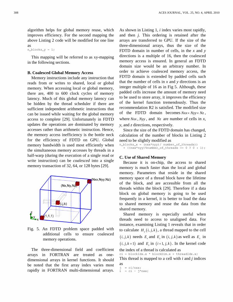
Fig. 5. An FDTD problem space padded with

additional cells to ensure coalesced memory operations.

The three-dimensional field and coefficient

arrays in FORTRAN are treated as one-dimensional arrays in kernel functions. It should be noted that the first array index varies most rapidly in FORTRAN multi-dimensional arrays.

As shown in Listing 1, i index varies most rapidly, and then j. This ordering is retained after the arrays are transferred to GPU. If the size of the three-dimensional arrays, thus the size of the FDTD domain in number of cells, in the x and y directions is a multiple of 16, then the coalesced memory access is ensured. In general an FDTD domain size would be an arbitrary number. In order to achieve coalesced memory access, the FDTD domain is extended by padded cells such that the number of cells in x and y directions is an integer multiple of 16 as in Fig 5. Although, these padded cells increase the amount of memory need to be used to store array, it improves the efficiency of the kernel function tremendously. Thus the recommendation R2 is satisfied. The modified size of the FDTD domain becomes Nxx Nyy Nz× × ,

where Nxx , Nyy , and Nz are number of cells in x,

y, and z directions, respectively. Since the size of the FDTD domain has changed,

calculation of the number of blocks in Listing 2 need to be slightly modified as n_blocks_x = (nxx*nyy)/ number_of_threads))

+ ((nxx*nyy)%number_of_threads == 0 ? 0 : 1);

C. Use of Shared Memory

Because it is on-chip, the access to shared memory is much faster than the local and global memory. Parameters that reside in the shared memory space of a thread block have the lifetime of the block, and are accessible from all the threads within the block [29]. Therefore if a data block on global memory is going to be used frequently in a kernel, it is better to load the data to shared memory and reuse the data from the shared memory.

Shared memory is especially useful when threads need to access to unaligned data. For instance, examining Listing 1 reveals that in order to calculate ( ), ,yH i j k , a thread mapped to the cell

( ), ,i j k needs xE and zE in ( ), ,i j k as well as xE in

( ), , 1i j k + and zE in ( )1, ,i j k+ . In the kernel code

the index of a thread is calculated as ci = blockIdx.x * blockDim.x + threadIdx.x; This thread is mapped to a cell with i and j indices as j = ci/nxx; i = ci - j*nxx;


A cell with indices (i+1, j, k) can be accessed by ci+1, a cell with indices (i, j+1, k) can be accessed by ci+nxx, and a cell with indices (i, j, k+1) can be accessed by ci+nxx*nyy. Access to (i, j+1, k) and (i, j, k+1) are coalesced, however (i+1, j, k) is not. If an access to a field component at a neighboring cell in the x direction is needed, i.e. ( )1, ,zE i j k+ while calculating ( ), ,yH i j k and

( )1, ,yE i j k+ while calculating ( ), ,zH i j k , then

shared memory can be used to load the data block mapped by the thread block, and then the neighboring field value is accessed from the shared memory. At this point one needs to use the CUDA function __syncthreads() to ensure that all threads in the block are synchronized; thus all necessary data is loaded to the shared memory before it is used by the neighboring threads.

As discussed above, uncoalesced memory accesses can be eliminated by using shared memory. However, a problem arises when accessing the neighboring cells’ data through shared memory. While loading the shared memory, each thread copies one element from the global memory to the shared memory. If the thread on the boundary of the thread block needs to access the data in the neighboring cell, this data will not be available since it has not been loaded to the shared memory. One way to overcome this problem is to load another set of data, which includes the neighboring cell’s data, to shared memory. In the presented implementation the size of the data allocation in the shared memory is extended by 16, and some of the threads in the thread block are used only to copy data from global memory to this extended section in the shared memory. Then, for instance, the piece of code that calls the kernel function to update magnetic field components would be as in Listing 3. The kernel function that updates magnetic field components based on xyz-mapping is shown in Listing 4. threads = dim3(block_dim_x, block_dim_y, 1); grid = dim3( n_blocks_x, n_blocks_y, 1); shared_mem_size = 2*sizeof(float)*number_of_threads; update_magnetic_fields_on_kernel

<<<grid, threads, shared_memory_size>>>

(nxx, nyy, nx, ny, nz, Ex, Ey, Ez, Hx, Hy, Hz, Chxh,Chyh,Chzh, Chxey, Chxez, Chyez, Chyex, Chzex, Chzey); Listing 3. CUDA code to call kernel function for magnetic field updates. __global__ void update_magnetic_fields_on_kernel(int nxx, int nyy, int nz, float *Ex, float *Ey, float *Ez, float *Hx, float *Hy, float *Hz, float *Chxh, float *Chyh, float *Chzh, float *Chxey, float *Chxez, float *Chyez, float *Chyex, float *Chzex, float *Chzey) { extern __shared__ float sEyz[]; float *sEy = (float*) sEyz; float *sEz = (float*) &sEy[blockDim.x+16]; // ci: cell index // si: index in shared memory array int ci = blockIdx.x * blockDim.x + threadIdx.x; int j = ci/nxx; int i = ci - j*nxx; int si = threadIdx.x; int sip1 = si+1; int nxxyy = nxx*nyy; int cizp; int ciyp; float ex; ci = ci + blockIdx.y*nxxyy; if (j < ny) { cizp = ci+nxxyy; ciyp = ci+nxx; ex = Ex[ci]; sEz[si] = Ez[ci]; sEy[si] = Ey[ci]; if (threadIdx.x<16) {

sEz[blockDim.x+threadIdx.x] = Ez[ci+blockDim.x]; sEy[blockDim.x+threadIdx.x] = Ey[ci+blockDim.x]; }

__syncthreads(); Hx[ci] = Chxh[ci] * Hx[ci] + Chxey[ci] * (Ey[cizp]-Ey[ci]) + Chxez[ci] * (Ez[ciyp]-sEz[si]); Hy[ci] = Chyh[ci] * Hy[ci]

+ Chyez[ci] * (sEz[sip1]-sEz[si]) + Chyex[ci] * ( Ex[cizp]-ex); Hz[ci] = Chzh[ci] * Hz[ci] + Chzex[ci] * (Ex[ciyp]-ex) + Chzey[ci] * (sEy[sip1]-sEy[si]); } }

Listing 4. CUDA code to update magnetic field components based on xyz-mapping.


D. Data Reuse As discussed above, the global memory access

affects the performance of a CUDA program significantly. Therefore, data transfers from and to the global memory should be avoided as much as possible. It may even be better to recalculate some data instead of recalling the data from global memory. If some data is already transferred from the global memory and it is available, it is better to use it as many times as possible. As can be observed from Listing 1, such data reuse is possible in an FDTD algorithm: while calculating

( ), ,xH i j k and ( ), ,yH i j k , ( ), , 1yE i j k + and

( ), , 1xE i j k + are used and the values of these

components are ready in the registers of the thread. If one increments the k index by one, these values will be reused to calculate ( ), , 1xH i j k + and

( ), , 1yH i j k + . Therefore, a kernel function can be

constructed based on the xy-mapping in which each thread traverses in the z direction in a for loop by incrementing k index of the cells. A kernel function based on xy-mapping can be coded as shown in Listing 5. __global__ void update_magnetic_fields_on_kernel(int nxx, int nyy, int nx, int ny, int nz, float *Ex, float *Ey, float *Ez, float *Hx, float *Hy, float *Hz, float *Chxh, float *Chyh, float *Chzh, float *Chxey, float *Chxez, float *Chyez, float *Chyex, float *Chzex, float *Chzey) { extern __shared__ float sEyz[]; float *sEy = (float*) sEyz; float *sEz = (float*) &sEy[blockDim.x+16]; int ci = blockIdx.x * blockDim.x + threadIdx.x; int j = ci/nxx; int i = ci - j*nxx; int si = threadIdx.x; int sip1 = si+1;

int nxxyy = nxx*nyy; int cizp; int cipnxx; float ey, eyzp; float ex, exzp; if (j < ny) { ey = Ey[ci]; ex = Ex[ci]; for (int k=0;k<nz;k++) { cizp = ci + nxxyy; exzp = Ex[cizp]; eyzp = Ey[cizp]; sEz[si] = Ez[ci]; if (threadIdx.x<16) {

sEz[blockDim.x+threadIdx.x] = Ez[ci+blockDim.x];

} __syncthreads(); Hx[ci] = Chxh[ci]*Hx[ci] + Chxey[ci]*(eyzp-ey) + Chxez[ci]*(Ez[ci+nxx]-sEz[si]); Hy[ci] = Chyh[ci] * Hy[ci] + Chyez[ci] * (sEz[sip1]-sEz[si]) + Chyex[ci] * (exzp-ex); sEy[si] = ey; if (threadIdx.x<16) {

sEy[blockDim.x+threadIdx.x] = Ey[ci+blockDim.x];

} __syncthreads(); Hz[ci] = Chzh[ci] * Hz[ci] + Chzex[ci] * (Ex[ci+nxx]-ex) + Chzey[ci] * (sEy[sip1]-sEy[si]); ci = cizp; ey = eyzp; ex = exzp; } } }

Listing 5. CUDA code to update magnetic field

components based on xy-mapping. At this point it should be noted that although the electric field updating equations are the same in form as the magnetic field updating equations, the implementation of kernels for electric field updates will be slightly different than those shown in Listings 4 and 5. The indices of the electric and magnetic field components adjacent to the FDTD domain boundaries and need to be updated are different as discussed in [3], and this difference need to be accounted for in the kernel implementations. Thus the implementations and also the performances of these kernels are slightly different. E. Optimization of Number of Threads As pointed out in recommendations R5 and R6, occupancy of the microprocessors and number of threads in a block are two other important parameters that affect the performance of a CUDA program. Number of threads and occupancy are tightly connected. It is possible to set the number of threads as a desired value while it may not be possible to control the occupancy; it is a function of number of threads, number of registers used in the kernel, amount of shared memory used by the


kernel, compute capability of the device, etc. A good practice is to optimize the number of threads while keeping the occupancy a reasonable value.

In order to determine optimum number of threads CUDA Visual Profiler is used: the kernel functions that update the electric and magnetic field components are run using different values of number of threads per block for both the xyz-mapping and xy-mapping algorithms, and the cpu times are recorded as they are captured by the CUDA Visual Profiler. For this test, an FDTD domain with size of 8 million cells (200 200 200)× × is used. The result of the

parameter sweep is shown in Fig. 6. It is found that for the magnetic field updates using xy-mapping algorithm performs the best with 512 threads per block, while electric field updates performs best with 128 threads per block. For the xyz-mapping both electric and magnetic field updates perform the best with 64 threads per block. These numbers are used in the subsequent performance analysis tests. From the figure it can be noticed that xy-mapping algorithm is faster than the xyz-mapping algorithm.

One can notice in Fig. 6 that, the cpu time is not shown for 448 and 512 number of threads for the electric field kernel using the xy-mapping. The number of registers for this kernel is 37 and occupancy becomes zero for large number of threads. Hence, the kernel cannot be run with 448 or 512 threads per block.

Fig. 6. CPU time versus number of threads per block.

V. PERFORMANCE ANALYSIS

The performance of the developed CUDA code for a general FDTD method as described before is examined as a function of problem size for both the xy-mapping and xyz-mapping algorithms. The analysis is performed on an NVIDIA® Tesla™ C1060 Computing Processor installed on a 64 bit Windows XP computer. This card has 240 streaming processor cores operating at 1.3 GHz. Size of a cubic FDTD problem domain has been swept and the number of million cells per second (NMCPS) processed is calculated as a measure of the performance of the CUDA program. Number of million cells is calculated as [20]

610steps

s

n Nx Ny NzNMCPS

t−× × ×

= × , (2)

where stepsn is the number of time steps the program

has been run and st is the total time of program run

in seconds. The result of the analysis is shown in Fig. 7. It can be observed that the xy-mapping algorithm processes about 450 million cells per second on the average while xyz-mapping algorithm processes 400 million cells per second.

Fig. 7. Algorithm speed versus problem size.

VI. CONCLUSION A CUDA implementation of FDTD method is

presented in this contribution. The FDTD formulation considered is for general dielectric media and conductive media and does not assume the same cell sizes in x, y, and z directions. Two thread-to-cell mapping algorithms are discussed and it is shown that the so referred to as xy-


mapping algorithm is better in terms of performance.

It should also be noted that each cell in the FDTD problem space can have a different material. If a limited number of materials are considered, the presented codes can be revised based on material indexed FDTD formulation, thus GPU constant memory space, which is faster than the global memory, can be utilized and a faster CUDA implementation for these FDTD formulations can be achieved.

REFERENCES [1] K. S. Yee, “Numerical Solution of Inital

Boundary Value Problems Involving Maxwell's Equations in Isotropic Media,” IEEE Transactions on Antennas and Propagation, vol. 14, pp. 302–307, May 1966.

[2] A. Taflove and S. C. Hagness, Computational Electrodynamics: The Finite-Difference Time-Domain Method, 3rd edition, Artech House, 2005.

[3] A. Elsherbeni and V. Demir, “The Finite Difference Time Domain Method for Electromagnetics: With MATLAB Simulations,” SciTech Publishing, 2009.

[4] S. E. Krakiwsky, L. E. Turner, and M. M. Okoniewski, “Graphics Processor Unit (GPU) Acceleration of Finite-Difference Time-Domain (FDTD) Algorithm,” Proc. 2004 International Symposium on Circuits and Systems, vol. 5, pp. V-265–V-268, May 2004.

[5] S. E. Krakiwsky, L. E. Turner, and M. M. Okoniewski, “Acceleration of Finite-Difference Time-Domain (FDTD) Using Graphics Processor Units (GPU),” 2004 IEEE MTT-S International Microwave Symposium Digest, vol. 2, pp. 1033–1036, June 2004.

[6] R. Schneider, S. Krakiwsky, L. Turner, and M. Okoniewski, “Advances in Hardware Acceleration for FDTD,” Ch. 20 in Computational Electrodynamics: The Finite-Difference Time-Domain Method, 3rd edition, Artech House, 2005.

[7] M. J. Inman, A. Z. Elsherbeni, and C. E. Smith “GPU Programming for FDTD Calculations,” The Applied Computational

Electromagnetics Society (ACES) Conference, 2005.

[8] M. J. Inman and A. Z. Elsherbeni, “Programming Video Cards for Computational Electromagnetics Applications,” IEEE Antennas and Propagation Magazine, vol. 47, no. 6, pp. 71–78, Dec. 2005.

[9] M. J. Inman and A. Z. Elsherbeni, “Acceleration of Field Computations Using Graphical Processing Units,” The Twelfth Biennial IEEE Conference on Electromagnetic Field Computation CEFC 2006, April 30 - May 3, 2006.

[10] M. J. Inman, A. Z. Elsherbeni, J. G. Maloney, and B. N. Baker, “Practical Implementation of a CPML Absorbing Boundary for GPU Accelerated FDTD Technique,” The 23rd Annual Review of Progress in Applied Computational Electromagnetics Society, 19-23 March 2007.

[11] S. Adams, J. Payne, and R. Boppana, “Finite Difference Time Domain (FDTD) Simulations Using Graphics Processors,” Proceedings of the 2007 DoD High Performance Computing Modernization Program Users Group (HPCMP) Conference, pp. 334–338, 2007.

[12] D. K. Price, J. R. Humphrey, and E. J. Kelmelis, “GPU-based Accelerated 2D and 3D FDTD Solvers,” in Physics and Simulation of Optoelectronic Devices XV, of Proceedings of SPIE, vol. 6468, Jan. 2007.

[13] D. K. Price, J. R. Humphrey, and E. J. Kelmelis, “Accelerated Simulators for Nano-Photonic Devices,” International Conference on Numerical Simulation of Optoelectronic Devices 2007, pp. 103–104, Sept. 2007.

[14] M. Inman, A. Elsherbeni, J. Maloney, and B. Baker, “Practical Implementation of a CPML Absorbing Boundary for GPU Accelerated FDTD Technique,” Applied Computational Electromagnetics Society Journal, vol. 23, no. 1, pp. 16–22, 2008.

[15] M. J. Inman and A. Z. Elsherbeni, “Optimization and parameter exploration using GPU based FDTD solvers,” IEEE MTT-S International Microwave Symposium Digest, pp. 149-152, June 2008.


[16] N. Takada, N. Masuda, T. Tanaka, Y. Abe, and T. Ito, “A GPU Implementation of the 2-D Finite-Difference Time-Domain Code Using High Level Shader Language,” Applied Computational Electromagnetics Society Journal, vol. 23, no. 4, pp. 309–316, 2008.

[17] A. Valcarce, G. de la Roche, and J. Zhang, “A GPU Approach to FDTD for Radio Coverage Prediction,” Proceedings of the 11th IEEE Singapore International Conference on Communication Systems (ICCS '08), pp. 1585–1590, Nov. 2008.

[18] P. Sypek and M. Michal, “Optimization of a FDTD Code for Graphical Processing Units,” 17th International Conference on Microwaves, Radar and Wireless Communications (MIKON), pp. 1–3, May 2008.

[19] A. Balevic, L. Rockstroh, A. Tausendfreund, S. Patzelt, G. Goch, and S. Simon, “Accelerating Simulations of Light Scattering Based on Finite-Difference Time-Domain Method with General Purpose GPUs,” Proceedings of the 2008 11th IEEE International Conference on Computational Science and Engineering, pp. 327–334, 2008.

[20] P. Sypek, A. Dziekonski, and M. Mrozowski, “How to Render FDTD Computations More Effective Using a Graphics Accelerator,” IEEE Transactions on Magnetics, vol. 45, no. 3, pp. 1324–1327, 2009.

[21] N. Takada, T. Shimobaba, N. Masuda, and T. Ito, “High-speed FDTD Simulation Algorithm for GPU with Compute Unified Device Architecture,” IEEE International Symposium on Antennas & Propagation & USNC/URSI National Radio Science Meeting,. 4, 2009.

[22] A. Valcarce, G. De La Roche, A. Jüttner, D. López-Pérez, and J. Zhang, “Applying FDTD to the coverage prediction of WiMAX femtocells,” EURASIP Journal on Wireless Communications and Networking, Feb. 2009.

[23] C. Ong, M. Weldon, D. Cyca, and M. Okoniewski, “Acceleration of Large-Scale FDTD Simulations on High Performance GPU Clusters,” 2009 IEEE International Symposium on Antennas & Propagation & USNC/URSI National Radio Science Meeting, 2009.

[24] M. J. Inman, A. Elsherbeni, and V. Demir, “Graphics Processing Unit Acceleration of Finite Difference Time Domain”, Ch. 12 in The Finite Difference Time Domain Method for Electromagnetics (with MATLAB Simulations), SciTech Publishing, 2009.

[25] I. Buck, Brook Spec v0.2, Stanford Univ. Press, 2003.

[26] NVIDIA CUDA ZONE, http://www.nvidia.com/object/cuda_home.html.

[27] CUDA 2.1 Quickstart Guide, http://www.nvidia.com/object/cuda_develop.html.

[28] J. A. Roden and S. Gedney, “Convolution PML (CPML): An Efficient FDTD Implementation of the CFS-PML for Arbitrary Media,” Microwave and Optical Technology Letters, vol. 27, no. 5, pp. 334–339, 2000.

[29] CUDA 2.1 Programming Guide, http://www.nvidia.com/object/cuda_develop.html.

[30] CUDA Best Practices Guide, http://www.nvidia.com/object/cuda_develop.html.

Veysel Demir is an Assistant Professor at The Department of Electrical Engineering, Northern Illinois University. He received his B.Sc. degree in electrical engineering from Middle East Technical University, Ankara, Turkey, in 1997. He studied at

Syracuse University, New York, where he received both a M.Sc. and Ph.D. in electrical engineering in 2002 and 2004, respectively. During his graduate studies, he worked as research assistant for Sonnet Software, Inc., Liverpool, New York. He worked as a visiting research scholar in the Department of Electrical Engineering at the University of Mississippi from 2004 to 2007. He joined Northern Illinois University in August 2007. His research interests include numerical analysis techniques as well as microwave and radiofrequency (RF) circuit analysis and design.


Dr. Demir is a member of IEEE and ACES and has coauthored more than 20 technical journal and conference papers. He is the coauthor of the books Electromagnetic Scattering Using the Iterative Multiregion Technique (Morgan & Claypool, 2007) and The Finite Difference Time Domain Method for Electromagnetics with MATLAB Simulations (Scitech 2009).

Atef Z. Elsherbeni is a Professor of Electrical Engineering and Associate Dean for Research and Graduate Programs, the Director of The School of Engineering CAD Lab, and the Associate Director of The

Center for Applied Electromagnetic Systems Research (CAESR) at The University of Mississippi. In 2004 he was appointed as an adjunct Professor, at The Department of Electrical Engineering and Computer Science of the L.C. Smith College of Engineering and Computer Science at Syracuse University. On 2009 he was selected as Finland Distinguished Professor by the Academy of Finland and Tekes.

Dr. Elsherbeni has conducted research dealing with scattering and diffraction by dielectric and metal objects, finite difference time domain analysis of passive and active microwave devices including planar transmission lines, field visualization and software development for EM education, interactions of electromagnetic waves with human body, sensors development for monitoring soil moisture, airports noise levels, air quality including haze and humidity, reflector and printed antennas and antenna arrays for radars, UAV, and personal communication systems, antennas for wideband applications, antenna and material properties measurements, and hardware and software acceleration of computational techniques for electromagentics.

Dr. Elsherbeni is the co-author of the book “The Finite Difference Time Domain Method for Electromagnetics With MATLAB Simulations”, SciTech 2009, the book “Antenna Design and Visualization Using Matlab”, SciTech, 2006, the book “MATLAB Simulations for Radar Systems Design”, CRC Press, 2003, the book

“Electromagnetic Scattering Using the Iterative Multiregion Technique”, Morgan & Claypool, 2007, the book “Electromagnetics and Antenna Optimization using Taguchi's Method”, Morgan & Claypool, 2007, and the main author of the chapters “Handheld Antennas” and “The Finite Difference Time Domain Technique for Microstrip Antennas” in Handbook of Antennas in Wireless Communications, CRC Press, 2001.

Dr. Elsherbeni is a Fellow member of the Institute of Electrical and Electronics Engineers (IEEE) and a Fellow member of The Applied Computational Electromagnetics Society (ACES). He is the Editor-in-Chief for ACES Journal and an Associate Editor to the Radio Science Journal.


Compute Unified Device Architecture (CUDA) Based … Terms—FDTD methods, parallel architectures,...

Documents

Transcript of Compute Unified Device Architecture (CUDA) Based … Terms—FDTD methods, parallel architectures,...