Computational Topology Counterexamples with 3D Visualization of

COMPUTATIONAL TOPOLOGY WITH REGINA:
ALGORITHMS, HEURISTICS AND IMPLEMENTATIONS
BENJAMIN A. BURTON
Dedicated to J. Hyam Rubinstein
Author’s self-archived versionAvailable from http://www.maths.uq.edu.au/~bab/papers/
Abstract. Regina is a software package for studying 3-manifold triangula-tions and normal surfaces. It includes a graphical user interface and Python
bindings, and also supports angle structures, census enumeration, combina-
torial recognition of triangulations, and high-level functions such as 3-sphererecognition, unknot recognition and connected sum decomposition.
This paper brings 3-manifold topologists up-to-date with Regina as it ap-
pears today, and documents for the first time in the literature some of the keyalgorithms, heuristics and implementations that are central to Regina’s perfor-
mance. These include the all-important simplification heuristics, key choices
of data structures and algorithms to alleviate bottlenecks in normal surfaceenumeration, modern implementations of 3-sphere recognition and connected
sum decomposition, and more. We also give some historical background forthe project, including the key role played by Rubinstein in its genesis 15 years
ago, and discuss current directions for future development.
1. Introduction
Algorithmic problems run to the heart of low-dimensional topology. Promi-nent amongst these are decision problems (e.g., recognising the unknot, or testingwhether two triangulated manifolds are homeomorphic); decomposition problems(e.g., decomposing a triangulated manifold into a connected sum of prime mani-folds); and recognition problems (e.g., “naming” the manifold described by a giventriangulation).
For 3-manifolds in particular, such problems typically have highly complex andexpensive solutions—running times are often exponential or super-exponential, andimplementations are often major endeavours developed over many years (if theyexist at all). This is in contrast to dimension two, where many such problems areeasily solved in small polynomial time, and dimensions ≥ 4, where such problemscan become provably undecidable [21, 40].
Regina [5, 14] is a software package for low-dimensional topologists and knottheorists. Its main focus is on triangulated 3-manifolds, though it is now branch-ing into both two and four dimensions also (see Section 7). It provides powerful
2000 Mathematics Subject Classification. Primary 57-04, 57N10; Secondary 68W05, 57Q15.Key words and phrases. 3-manifolds, algorithms, software, simplification, normal surfaces,
recognition, angle structures.The author is supported by the Australian Research Council under the Discovery Projects
funding scheme (projects DP1094516 and DP110101104).
1

2 BENJAMIN A. BURTON
algorithms and heuristics to assist with decision, decomposition and recognitionproblems; more broadly, it includes a range of facilities to study and manipulate3-manifold triangulations. It offers rich support for normal surface theory, a majoralgorithmic framework that recurs throughout 3-manifold topology.
One of Regina’s most important uses is for experimentation: it can analyse asingle example too large to study by hand, or millions of examples “in bulk”. Otheruses include computer proofs, such as the recent resolution of Thurston’s old ques-tion of whether the Weber-Seifert dodecahedral space is non-Haken [18], and calcu-lation of previously-unknown topological invariants, such as recent improvementsto crosscap numbers in knot tables [13, 15].
The remainder of this introduction gives a brief overview of Regina and somehistory behind its early development, back to its genesis with Rubinstein 15 yearsago. Following this, we select some of Regina’s most important features and studythe modern heuristics, algorithms and implementations behind them. Some ofthese details are crucial for Regina’s fast performance, but have not appeared inthe literature to date. Overall, this paper offers a fresh update on the significantprogress and performance enhancements in the eight years since Regina’s last majorreport in the literature [5].
The specific features that we focus on are:
• the process of simplifying triangulations, which plays a critical role in manyof Regina’s high-level algorithms;• the enumeration of normal and almost normal surfaces, including the high-
level 0-efficiency, 3-sphere recognition and connected sum decompositionalgorithms;• combinatorial recognition, whereby Regina attempts to recognise a trian-
gulation by studying its combinatorial structure;• the enumeration of angle structures, taut angle structures and veering struc-
tures on triangulations.
With respect to these features, there are interesting new developments in thepipeline. Examples include “breadth-first simplification” of triangulations, the treetraversal algorithm for enumerating vertex normal surfaces, and new 0-efficiencyand 3-sphere recognition algorithms based on linear programming that exhibit ex-perimental polynomial-time behaviour. The corresponding code is already written(it is now being tested and prepared for integration into Regina), and we outlinethese new developments in the relevant sections of this paper.
To finish, Section 6 gives concrete examples of how Regina can be used forexperimentation, including an introduction to Regina’s in-built Python scripting, sothat interested readers can use these as launching points for their own experiments.Section 7 concludes with additional future directions for Regina, including newwork with Ryan Budney on triangulated 4-manifolds, much of which is alreadycoded and running in the development repository.
1.1. Overview of Regina. Regina is now 13 years old, with over 190 000 lines ofsource code. It is released under the GNU General Public License, and contribu-tions from the research community are welcome. It adheres to the following broaddevelopment principles, in order of precedence:
(1) Correctness: Having correct output is critical, particularly for applicationssuch as computer proofs. Regina is extremely conservative in this regard:

COMPUTATIONAL TOPOLOGY WITH REGINA 3
for example, it will use arbitrary precision integer arithmetic if it cannotbe proven unnecessary, and the API documentation makes thorough use ofpreconditions and postconditions.
(2) Generality: Algorithms operate in the broadest possible scenarios (withinreason), and do not require preconditions that cannot be easily tested. Forinstance, unknot recognition runs correctly for both bounded and idealtriangulations, and even when the input triangulation is not known to bea knot complement (whereupon it generalises to solid torus recognition).
(3) Speed: Because many of its algorithms run in exponential or super-exponen-tial time, speed is imperative. Regina makes use of sophisticated algorithmsand heuristics that, whilst adhering to the constraints of correctness andgenerality, make it practical for real topological problems.
Regina is multi-platform, and offers a drag-and-drop installer for MacOS, anMSI-based installer for Windows, and ready-made packages for several GNU/Linuxdistributions. It is thoroughly documented, and stores its data files in a compressedXML format. Regina provides three levels of user interface:
• a full graphical user interface, based on the Qt framework [48];• a scripting interface based on Python, which can interact with the graphical
interface or be used a standalone Python module;• a programmers’ interface offering native access to Regina’s mathematical
core through a C++ shared library.
There are facilities to help new users learn their way around, including an illus-trated users’ handbook, context-sensitive “what’s this?” help, and sample data filesthat can be opened through the File −→Open Example menu.
Regina’s core strengths are in working with triangulations, normal surfacesand angle structures. It only offers basic support for hyperbolic geometries, forwhich the software packages SnapPea [60] and its successor SnapPy [23] are moresuitable. In addition to its range of low-level operations and 3-manifold invari-ants, Regina includes implementations of high-level decision and decompositionalgorithms, including the only known full implementations of 3-sphere recogni-tion and connected sum decomposition. For a comprehensive list of features, seehttp://regina.sourceforge.net/docs/featureset.html.
1.2. History. In the 1990s, Jeff Weeks’ software package SnapPea had openedup enormous possibilities for computer experimentation with hyperbolic 3-mani-folds. In contrast, outside the hyperbolic world many fundamental 3-manifoldalgorithms remained purely theoretical, including high-profile algorithms such as3-sphere recognition, connected sum decomposition, Haken’s unknot recognitionalgorithm, and testing for incompressible surfaces.
More broadly, normal surface theory—a ubiquitous technology in algorithmic3-manifold topology—had no concrete software implementation (or at least nonethat had been publicised). Many of the algorithms that used normal surfaces wereso complex that it was believed that any attempt at implementation would be bothpainstaking to develop and impractically slow to run.
Nevertheless, Rubinstein sought to move these algorithms from the theoreticalrealm to the practical, and in 1997 he assembled a team for a new software projectthat would make computational normal surface theory a reality. This initial teamconsisted of David Letscher, Richard Rannard, and myself. Much planning was

4 BENJAMIN A. BURTON
done and a little preliminary code was written, but then the team members becameoccupied with different projects.
Letscher later resumed the project on his own, and at a 1999 workshop on com-putational 3-manifold topology at Oklahoma State University he presented Normal,a Java-based application that could modify and simplify triangulations, and enu-merate vertex normal surfaces. This was an exciting development, but the softwarewas proof-of-concept only, and later that month Letscher and I sat down to beginagain from scratch. The successor would be a fast and robust software packagewith a C++ engine, would be designed for extensibility and portability, and wouldsupport community-contributed “add-ons”.
Letscher stayed with the project for the first year, and then moved on to pursuedifferent endeavours. I remained with the project (a PhD student at the time, withmore time on my hands), and the project—now known as Regina—saw its firstpublic release in December 2000. Development at this stage was taking place atOklahoma State University, where Bus Jaco was both a strong supporter and asignificant influence on the project in its formative years.
Around that time, a significant phase shift was taking place in normal surfacetheory: Jaco and Rubinstein were developing their theory of 0-efficient triangula-tions. Their landmark 2003 paper [33] showed that key problems such as 3-sphererecognition and connected sum decomposition could be solved without the expen-sive and highly problematic operation of cutting along a normal surface, and thatinstead this could be replaced by a crushing operation that always reduces thenumber of tetrahedra. For the first time, the key algorithms of 3-sphere recognitionand connected sum decomposition became both feasible and practical to imple-ment. Shortly after, in March 2004, Regina became the first software package toimplement robust, conclusive solutions to these fundamental problems.
Regina has come a long way since development began in 1999. It continues togrow in its mathematics, performance, usability, and technical infrastructure, and itenjoys contributions from a wide range of people (as noted in the following section).For a list of highlights over the years, the reader is invited to peruse the “abbreviatedchangelog” at http://regina.sourceforge.net/docs/history.html.
1.3. Acknowledgements. Regina is a mature project and has benefited from theexpertise of many people and the resources of many organisations.
Ryan Budney and William Pettersson have both made significant and ongoingcontributions, and are both now primary developers for the project. A host of otherpeople have contributed either code or expertise, including Bernard Blackham,Marc Culler, Dominique Devriese, Nathan Dunfield, Matthias Goerner, WilliamJaco, David Letscher, Craig Macintyre, Melih Ozlen, Hyam Rubinstein, JonathanShewchuk, and Stephan Tillmann. In addition, the open-source software librariesNormaliz [3] (by Winfried Bruns, Bogdan Ichim and Christof Soeger) and SnapPea[60] (by Jeff Weeks) have been grafted directly into Regina’s calculation engine.
Organisations that have contributed to the development of Regina include theAmerican Institute of Mathematics, the Australian Research Council (DiscoveryProjects DP0208490, DP1094516 and DP110101104), the Institute for the Physicsand Mathematics of the Universe (University of Tokyo), Oklahoma State University,the Queensland Cyber Infrastructure Foundation, RMIT University, the Universityof Melbourne, The University of Queensland, the University of Victoria (Canada),and the Victorian Partnership for Advanced Computing (Australia).

COMPUTATIONAL TOPOLOGY WITH REGINA 5
2. Simplifying triangulations
The most basic object in Regina is a 3-manifold triangulation. Regina doesnot restrict itself to simplicial complexes; instead it uses generalised triangulations,a broader notion that can represent a rich array of 3-manifolds using very fewtetrahedra, as described in Section 2.1 below.
One of Regina’s most important functions is simplification: retriangulating a 3-manifold to use very few tetrahedra (ideally, the fewest possible). Regina includesa rich array of local simplification moves, as outlined in Section 2.2; together itcombines these moves into a strong simplification algorithm, which we describe infull in Section 2.3. Moreover, this algorithm is fast: in Section 2.4 we outline someimportant implementation details, and show that it runs in small polynomial time.
This simplification algorithm gives no guarantee of achieving a minimal trian-gulation (where the number of tetrahedra is the smallest possible). However, thealgorithm is extremely powerful in practice: for instance, of the 652 635 906 combi-natorially distinct triangulations of the 3-sphere with 3 ≤ n ≤ 10 tetrahedra [10],this simplification algorithm quickly reduces all but 26 of them.
Having a powerful simplification algorithm is essential in computational 3-ma-nifold topology, for several reasons:
• Many significant algorithms have running times that are exponential orworse in the number of tetrahedra, and so reducing this number is of greatpractical importance.• Good simplification may allow us to avoid these expensive algorithms en-
tirely. For instance, in 3-sphere recognition we could simplify the triangu-lation and then compare it to the known trivial (≤ 2-tetrahedron) triangu-lations of S3: if they match then the expensive steps involving normal andalmost normal surfaces can be avoided altogether [12].• More generally, simplification offers good heuristics for solving the home-
omorphism problem. Simplified triangulations are often well-structured,which makes Regina’s combinatorial recognition routines more likely toidentify the underlying 3-manifold (see Section 4). Moreover, if two trian-gulations T and T ′ represent the same 3-manifold, then after simplificationit often becomes relatively easy to convert one into the other using Pachnermoves (i.e., bistellar flips) [12].
Most of the individual local moves that we describe in Section 2.2 are well-known, and were implemented by Letscher in his early software package Normal.Moreover, Matveev [43, 46] and Martelli and Petronio [41] perform similar movesin the dual setting of special spines, and the author has described several in thecontext of census enumeration [4]. We therefore outline these moves very briefly,although in our general setting there are prerequisites for preserving the underlying3-manifold that earlier authors have not required (either because they worked inthe more flexible dual setting of spines, or they were simply proving criteria forminimality and/or irreducibility). We pay particular attention to the edge collapsemove, whose prerequisites are complex and require non-trivial algorithms to testquickly. The combined simplification algorithm, whose underlying heuristics havebeen fine-tuned over many years, is described here in Section 2.3 for the first time.
In Section 2.5, we conclude our discussion on simplification with a new technol-ogy that will soon make its way into Regina: simplification by breadth-first search

6 BENJAMIN A. BURTONPSfrag
00
0
11
1
22
2
33
3
Tetrahedron 0 Tetrahedron 1
Figure 1. A triangulation of the real projective space RP 3
through the Pachner graph. Unlike the algorithm of Section 2.3, this is not polyno-mial-time; however, it is found to be extremely effective in handling the (very rare)pathological triangulations that cannot be simplified otherwise.
2.1. Generalised triangulations. A generalised 3-manifold triangulation, or justa triangulation from here on, is formed from n tetrahedra by affinely identifying(or “gluing”) some or all of their 4n faces in pairs. A face is allowed to be identifiedwith another face of the same tetrahedron. It is possible that several edges of asingle tetrahedron may be identified together as a consequence of the face gluings,and likewise for vertices. It is common to work with one-vertex triangulations, inwhich all vertices of all tetrahedra become identified as a single point.
Generalised triangulations can produce rich constructions with very few tetra-hedra. For instance, Matveev obtains 103 042 distinct closed orientable irreducible3-manifolds from just ≤ 13 tetrahedra [44], including representatives from all ofThurston’s geometries except for S2 × R (which cannot yield a manifold of thistype [54]).
Figure 1 illustrates a two-tetrahedron triangulation of the real projective spaceRP 3. The two tetrahedra are labelled 0 and 1, and the four vertices of each tetra-hedron are labelled 0, 1, 2 and 3. Faces 012 and 013 of tetrahedron 0 are joineddirectly to faces 012 and 013 of tetrahedron 1, creating a solid ball; then faces 023and 123 of tetrahedron 0 are joined to faces 132 and 032 of tetrahedron 1, effectivelygluing the top of the ball to the bottom of the ball with a 180◦ twist.
All of this information can be encoded in a table of face gluings, which is howRegina represents triangulations:
Tetrahedron Face 012 Face 013 Face 023 Face 123
0 1 (012) 1 (013) 1 (132) 1 (032)1 0 (012) 0 (013) 0 (132) 0 (032)
Consider the cell in the row for tetrahedron t and the column for face abc. Ifthis cell contains u (xyz ), this indicates that face abc of tetrahedron t is identifiedwith face xyz of tetrahedron u, using the affine gluing that maps vertices a, b andc of tetrahedron t to vertices x, y and z of tetrahedron u respectively.
For any vertex V of a triangulation, the link of V is defined as the frontier of asmall regular neighbourhood of V . This mirrors the traditional concept of a linkin a simplicial complex, but is modified to support the generalised triangulationsthat we use in Regina.
A closed triangulation is one that represents a closed 3-manifold (like the exampleabove): every tetrahedron face must be glued to a partner, and every vertex linkmust be a 2-sphere. A bounded triangulation is one that represents a 3-manifoldwith boundary: some tetrahedron faces are not glued to anything (together theseform the boundary of the manifold), and every vertex link must be a 2-sphere or a

COMPUTATIONAL TOPOLOGY WITH REGINA 7
(a) The 2-3 and 3-2 Pachner moves (b) The “aggregate” 4-4 move
Figure 2. Three Pachner-type moves
disc. In either case, it is important that no edge be identified with itself in reverseas a consequence of the face gluings.
Regina can also work with ideal triangulations, such as Thurston’s famous two-tetrahedron triangulation of the figure eight knot complement [58]: these are trian-gulations in which vertex links can be higher-genus closed surfaces. For simplicity,in this paper we focus our attention on closed and bounded triangulations only,though most of our results apply equally well to ideal triangulations also.
Users can enter tetrahedron gluings directly into Regina, or create triangulationsin other ways: importing from SnapPea [60] or other file formats; building “pre-packaged” constructions such as layered lens spaces or Seifert fibred spaces; enteringdehydration strings [20] or the more flexible isomorphism signatures [12] (shortpieces of text that completely encode a triangulation); or accessing large ready-made censuses that hold tens of thousands of triangulations of various types.
2.2. Individual simplification moves. In this section we outline several indi-vidual local moves on triangulations. Following this, in Section 2.3 we piece thesemoves together to build Regina’s full simplification algorithm.
We describe each move in full generality, as applied to either closed or boundedtriangulations, and without any restrictions such as orientability or irreducibility.For each move we give sufficient conditions under which the move is “safe”, i.e.,does not change the underlying 3-manifold.
To keep the exposition as short as possible, we simply state these conditionswithout proof. However, the proofs are simple: the key idea is that, throughoutthe intermediate stages of each move, we never crush an edge, flatten a bigon orflatten a triangular pillow whose bounding vertices, edges or faces respectively areeither identified or both in the boundary. For detailed examples of these types ofarguments, see (for instance) the proof of Lemma 3.7 in [6].
2.2.1. Pachner-type moves. Our first moves are simple combinations of the well-known Pachner moves [49], also known as bistellar flips. All of these moves,when performed locally within some larger triangulation, preserve the underlying3-manifold with no special preconditions required.
Definition 2.1. Consider a triangular bipyramid: this can be triangulated with(i) two distinct tetrahedra joined along an internal face, or with (ii) three distincttetrahedra joined along an internal degree three edge, as illustrated in Figure 2(a).A 2-3 Pachner move replaces (i) with (ii), and a 3-2 Pachner move replaces (ii)with (i).

8 BENJAMIN A. BURTON
(a) The 2-0 vertex move
gh
(b) The 2-0 edge move
∆
∆′
(c) The 2-1 edge move
Figure 3. Local moves around low-degree edges and vertices
Consider a square bipyramid (i.e., an octahedron). This can be triangulated withfour distinct tetrahedra joined along an internal degree four edge; moreover, thereare three ways of doing this (since the internal edge could follow any of the threemain diagonals of the octahedron). A 4-4 move replaces one such triangulationwith another, as illustrated in Figure 2(b).
There are two additional Pachner moves: the 1-4 move and the 4-1 move. Reginadoes not use either of these: the 1-4 move complicates the triangulation more thanis necessary (since it introduces a new vertex, which is never needed to simplifya triangulation [42, 43]), and the 4-1 move is a special case of an edge collapse(described later in this section). The 4-4 move is not a Pachner move, but it canbe expressed as an “aggregate” of a 2-3 move followed by a 3-2 move.
2.2.2. Moves around low-degree edges and vertices. It is well-known that (under theright conditions) minimal triangulations cannot have low-degree edges or vertices.One typically proves this using local moves around such edges or vertices that eitherreduce the number of tetrahedra or break some prior assumption on the manifold.
Here we outline three such moves, which Regina uses in a more general settingto simplify arbitrary triangulations. Unlike the earlier Pachner-type moves, thesemoves might change the underlying 3-manifold; after describing the moves, we listsufficient conditions under which they are “safe” (i.e., the 3-manifold is preserved).
Definition 2.2. A 2-0 vertex move operates on a triangular pillow formed fromtwo distinct tetrahedra surrounding an internal degree two vertex, as illustratedin Figure 3(a), and flattens this pillow to a single face. A 2-0 edge move operateson a bigon bipyramid formed from two distinct tetrahedra surrounding an internaldegree two edge, as illustrated in Figure 3(b), and flattens this to a pair of faces.
Consider a tetrahedron ∆, two of whose faces are folded together around aninternal degree one edge, and let ∆′ be some distinct adjacent tetrahedron as il-lustrated in Figure 3(c) (for clarity, the vertices of both tetrahedra are marked inbold). A 2-1 edge move flattens the two uppermost faces of ∆′ together and retri-angulates the remaining region with a single tetrahedron to yield a new degree oneedge, as shown in the illustration.
To ensure that these moves do not change the underlying 3-manifold, the follow-ing conditions are sufficient:
• For the 2-0 vertex move, the two faces that bound the pillow must bedistinct (i.e., not identified) and not both simultaneously in the boundary.
COMPUTATIONAL TOPOLOGY WITH REGINA 9
F
(a) The book opening and closing moves
∆
(b) One type of boundary shelling move
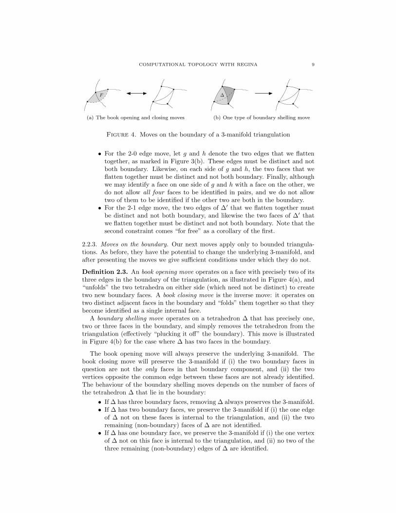
Figure 4. Moves on the boundary of a 3-manifold triangulation
• For the 2-0 edge move, let g and h denote the two edges that we flattentogether, as marked in Figure 3(b). These edges must be distinct and notboth boundary. Likewise, on each side of g and h, the two faces that weflatten together must be distinct and not both boundary. Finally, althoughwe may identify a face on one side of g and h with a face on the other, wedo not allow all four faces to be identified in pairs, and we do not allowtwo of them to be identified if the other two are both in the boundary.• For the 2-1 edge move, the two edges of ∆′ that we flatten together must
be distinct and not both boundary, and likewise the two faces of ∆′ thatwe flatten together must be distinct and not both boundary. Note that thesecond constraint comes “for free” as a corollary of the first.
2.2.3. Moves on the boundary. Our next moves apply only to bounded triangula-tions. As before, they have the potential to change the underlying 3-manifold, andafter presenting the moves we give sufficient conditions under which they do not.
Definition 2.3. An book opening move operates on a face with precisely two of itsthree edges in the boundary of the triangulation, as illustrated in Figure 4(a), and“unfolds” the two tetrahedra on either side (which need not be distinct) to createtwo new boundary faces. A book closing move is the inverse move: it operates ontwo distinct adjacent faces in the boundary and “folds” them together so that theybecome identified as a single internal face.
A boundary shelling move operates on a tetrahedron ∆ that has precisely one,two or three faces in the boundary, and simply removes the tetrahedron from thetriangulation (effectively “plucking it off” the boundary). This move is illustratedin Figure 4(b) for the case where ∆ has two faces in the boundary.
The book opening move will always preserve the underlying 3-manifold. Thebook closing move will preserve the 3-manifold if (i) the two boundary faces inquestion are not the only faces in that boundary component, and (ii) the twovertices opposite the common edge between these faces are not already identified.The behaviour of the boundary shelling moves depends on the number of faces ofthe tetrahedron ∆ that lie in the boundary:
• If ∆ has three boundary faces, removing ∆ always preserves the 3-manifold.• If ∆ has two boundary faces, we preserve the 3-manifold if (i) the one edge
of ∆ not on these faces is internal to the triangulation, and (ii) the tworemaining (non-boundary) faces of ∆ are not identified.• If ∆ has one boundary face, we preserve the 3-manifold if (i) the one vertex
of ∆ not on this face is internal to the triangulation, and (ii) no two of thethree remaining (non-boundary) edges of ∆ are identified.

10 BENJAMIN A. BURTON
e
V
W
∆1 ∆2
gi
hi
gi+1
hi+1
Figure 5. Collapsing an edge of a triangulation
2.2.4. Collapsing edges. Our final move is the most powerful: it collapses an edgeof the triangulation to a single point, and if the edge has high degree then it caneliminate many tetrahedra. The conditions for preserving the underlying 3-manifoldare complex, both to describe and to test algorithmically. The details are as follows.
Definition 2.4. An edge collapse operates on an edge e of the triangulation thatjoins two distinct vertices. It crushes edge e to a point and flattens every tetrahe-dron containing e to a face, as illustrated in Figure 5.
Suppose the edge e has degree d: we denote the d tetrahedra that contain it by∆1, . . . ,∆d, and we denote the two endpoints of e by V and W .
If e is an internal edge of the triangulation (i.e., its endpoints may lie on theboundary but its relative interior must not), then the following conditions are suf-ficient to preserve the underlying 3-manifold. Section 2.4 gives details on how wecan test these conditions efficiently.
(1) The tetrahedra ∆1, . . . ,∆d must all be distinct.(2) The two endpoints V and W (which we already know to be distinct) must
not both be in the boundary.(3) Denote the d “upper” edges in the diagram that touch V by g1, . . . , gd,
and denote the corresponding “lower” edges that touch W by h1, . . . , hd(so each gi, hi pair will be merged together by the edge collapse). We forma multigraph Γ (allowing loops and/or multiple edges) as follows:• each distinct edge of the triangulation becomes a node of Γ;• for each i = 1, . . . , d, we add an arc of Γ between the two nodes
corresponding to edges gi and hi;• we add an extra node ∂ to represent the boundary, and add an arc
from ∂ to every node that represents a boundary edge.Then this multigraph Γ must not contain any cycles.
(4) In a similar way, we build a multigraph whose nodes represent faces of thetriangulation, whose arcs join corresponding “upper” and “lower” faces thattouch V and W respectively, and with an extra boundary node connected toevery boundary face. Again, this multigraph must not contain any cycles.
In essence, condition (3) ensures that we never flatten a chain of bigons whoseoutermost edges are both identified or both boundary, and condition (4) ensuresthat we never flatten a chain of triangular pillows whose outermost faces are bothidentified or both boundary.
COMPUTATIONAL TOPOLOGY WITH REGINA 11
If the edge e lies in the boundary of the triangulation then we may still be able toperform the move: the sufficient conditions for preserving the 3-manifold are similarbut slightly more complex, and we refer the reader to Regina’s well-documentedsource code for the details.
2.3. The full simplification algorithm. Now that we are equipped with oursuite of local simplification moves, we can present the full details of Regina’s sim-plification algorithm. This algorithm is designed to be both fast and effective, inthat order of priority, and its underlying mechanics have evolved over many yearsaccording to what has been found to work well in practice.
Of course, other software packages—such as SnapPea [60] and the 3-ManifoldRecogniser [45]—have simplification algorithms of their own. To date there hasbeen no comprehensive comparison between them; indeed, such a comparison wouldbe difficult given the ever-present trade-off between speed and effectiveness.
Algorithm 2.5. Given an input triangulation T , the following procedure attemptsto reduce the number of tetrahedra in T without changing the underlying 3-manifold:
(1) Greedily reduce the number of tetrahedra as far as possible. We do this byrepeatedly applying the following moves, in the following order of priority,until no such moves are possible:• edge collapses;• low-degree edge moves (3-2 Pachner moves, or 2-0 or 2-1 edge moves);• low-degree vertex moves (2-0 vertex moves);• boundary shelling moves.
(2) Make up to 5R successive random 4-4 moves, where R is the maximumnumber of available 4-4 moves that could be made from any single triangu-lation obtained during this particular iteration of step (2). If we ever reacha triangulation from which we can greedily reduce the number of tetrahedra(as defined above) then return immediately to step (1).
(3) If the triangulation has boundary, then perform book opening moves untilno more are possible. If this enables us to collapse an edge then do so andreturn to step (1). Otherwise undo the book openings and continue.
(4) If a book closing move can be performed, then do it and return to step (1).Otherwise terminate the algorithm.
The greedy reduction in step (1) prioritises edge collapses, because these canremove many tetrahedra at once, and because we typically aim for a one-vertextriangulation. In step (2), the coefficient 5 is chosen somewhat arbitrarily; notealso that the quantity R might increase as this step progresses. The book openingsin step (3) aim to increase the number of vertices without adding new tetrahedra,in the hope that an edge collapse becomes possible. The book closures in step (4)aim to leave us with the smallest boundary possible, which becomes advantageousduring other expensive algorithms (such as normal surface enumeration).
Note that we never explicitly increase the number of tetrahedra (e.g., we neverperform an explicit 2-3 Pachner move). This is only possible because we have alarge suite of moves available: if we reformulate our algorithm in terms of Pachnermoves alone then almost every step would require both 2-3 and 3-2 moves.
One of the more prominent simplification techniques that we do not use is the0-efficiency reduction of Jaco and Rubinstein [33]. This is because the best knownalgorithms for testing for 0-efficiency run in worst-case exponential time. Moreover,
12 BENJAMIN A. BURTON
experimental observation suggests that—ignoring well-known exceptions, such asreducible manifolds and RP 3—after running Algorithm 2.5 we typically find thatthe triangulation is already 0-efficient. We discuss algorithms for 0-efficiency testingfurther in Section 3.3.
2.4. Time complexity and performance. Simplification is one of the most com-monly used “large-scale” routines in Regina’s codebase, and it is imperative thatit runs quickly. In this section we analyse the running time, which includes a dis-cussion of key implementation details for the edge collapse. All time complexitiesare based on the word RAM model of computation (so, for instance, adding twointegers is considered O(1) time as long as the integers only require log n bits).
Throughout this discussion, we let n denote the number of tetrahedra in thetriangulation. Some key points to note:
• Adding a new tetrahedron takes O(1) time. However, deleting a tetrahedrontakes O(n) time for Regina since we must reindex the tetrahedra that re-main (i.e., if we delete tetrahedron ∆i then we must rename ∆j to ∆j−1 forall j > i).1 Deleting many tetrahedra can be done in combined O(n) time,since if we are careful in our implementation then each leftover tetrahedrononly needs to be reindexed at most once.• Computing the skeleton of the triangulation (i.e., identifying and indexing
the distinct vertices, edges, faces and boundary components of the trian-gulation, and linking these to and from the corresponding tetrahedra) canbe done in O(n) time using standard depth-first search techniques.
Theorem 2.6. Algorithm 2.5 (the full simplification algorithm) runs in time O(n4 log n),where n is the number of tetrahedra in the input triangulation.
The worst culprit in raising the time complexity is the edge collapse move, andspecifically, testing its sufficient conditions. In practice running times are muchfaster than quartic, and with more delicacy we could bring down the theoreticaltime complexity to reflect this; we return to such issues after the proof.
Proof. First, we observe that for every move type except for the edge collapse, wecan test the sufficient conditions in O(1) time and perform the move in O(n) time(where the dominating factor is deleting tetrahedra and rebuilding the skeleton, asoutlined above).
For the edge collapse move, performing the move takes O(n) time but testingthe sufficient conditions is a little slower. Recall that we must build a multigraph Γand ensure that it contains no cycles. We can do this by adding one arc at a time,and tracking connected components: if an arc joins two distinct components thenwe merge them into a single component, and if an arc joins some component withitself then we obtain a cycle and the sufficient conditions fail.
To track connected components, we use the well-known union-find data structure[22]. With union-find, the operations of (i) identifying which component a nodebelongs to and (ii) merging two components together each take O(log n) time.Therefore testing the multigraph Γ for cycles takes O(n log n) time overall, andtesting sufficient conditions for an edge collapse likewise becomes O(n log n).
1This is Regina’s own implementation constraint: many moves could be O(1) if we ignoredRegina’s need to consecutively index tetrahedra and other objects. Either way, however, the time
complexity for the edge collapse—and hence the full simplification algorithm—would be the same.

COMPUTATIONAL TOPOLOGY WITH REGINA 13
From here the running time is simple to obtain. The algorithm works through“stages”, where in each stage we either reduce the number of tetrahedra, or wereduce the number of boundary faces through a book closing move. Either way, itis clear there can be at most O(n) such stages in total (since the triangulation andits boundary cannot disappear entirely).
Within each stage we perform O(n) moves in total: at most 5R ≤ 5(# edges) ≤5 · 6n successive 4-4 moves, and at most (# internal faces) ≤ 2n successive bookopening moves. This gives us a total of O(n2) moves throughout the life of thealgorithm, each requiring O(n) time to perform.
Between each pair of moves, we might test a large number of potential moveswhose sufficient conditions ultimately fail. The number of moves that we test ona given triangulation is clearly O(n) (since there are O(n) possible “local regions”in which each type of move could be performed), and so throughout the entirealgorithm with its O(n2) moves we run a total of O(n3) tests. In the worst case(edge collapses), each test could take O(n log n) time.
It is clear now that the total time spent performing moves is O(n3) and the totaltime spent testing sufficient conditions is O(n4 log n), yielding a running time ofO(n4 log n) overall. �
Some further remarks on this running time:
• We noted earlier that in practice running times are faster than O(n4 log n).This is because the powerful edge collapse moves typically reach the fewestpossible number of vertices very quickly (i.e., one vertex for a closed man-ifold, or else one vertex for each boundary component). Once we achievethis, testing sufficient conditions for an edge collapse move becomes O(1)time, which eliminates an n log n factor from our running time.• In theory, we can remove a factor of n as follows: once greedy simplification
fails and we move on to steps (2) and (3), we only test for new simplificationmoves in the immediate neighbourhood of the last 4-4 or book openingmove. The implementation becomes more subtle and the bookkeeping morecomplex, and this is planned for future versions of Regina.• Finally, we note that the log n factor can be stripped down to “almost
constant”: essentially an inverse of the Ackermann function, and ≤ 4 in allconceivable situations. We can do this by applying the path compressionoptimisation to the union-find data structure; see [22, 56] for details.
We finish this section with a practical demonstration. Let T be the 23-tetra-hedron triangulation of the Weber-Seifert dodecahedral space presented in [18], andlet S be an arbitrarily-chosen vertex normal surface of the highest possible genus(here we choose vertex surface #1733, which is an orientable genus 16 surface). Ifwe cut T open along the surface S using Regina’s cutAlong() procedure, we obtaina (disconnected) bounded triangulation T ′ with 1990 tetrahedra. The simplificationalgorithm reduces this to 135 tetrahedra in roughly 1.9 seconds (as measured on a2.93 GHz Intel Core i7).
If we perform a barycentric subdivision on T ′, we obtain a new triangulation T ′′with 47 760 tetrahedra (and a large number of vertices, which means a large numberof expensive edge collapse moves). Again the simplification algorithm reduces thisto 135 tetrahedra, but this time takes 780 seconds, suggesting (for this arbitraryexample) only a quadratic—not quartic—growth rate in n.

14 BENJAMIN A. BURTON
2.5. Exhaustive simplification via the Pachner graph. We finish our dis-cussion on simplification with a new technology: breadth-first search through thePachner graph. The key idea is, instead of using greedy simplification heuristics,to try all possible sequences of Pachner moves (up to a user-specified limit). Theresult is a much slower, but also much stronger, simplification algorithm. This algo-rithm is based on ideas from the large-scale experimental study of Pachner graphsdescribed in [12], and the code will soon be merged into Regina’s main source tree.
Definition 2.7. For a closed 3-manifold triangulation M, the restricted Pachnergraph P1(M) is the infinite graph whose nodes correspond to isomorphism classesof one-vertex triangulations of M (where by isomorphism we mean a relabellingof tetrahedra and/or their vertices), and where two nodes are joined by an arc ifthere is a 2-3 or 3-2 Pachner move between the corresponding triangulations. Thenodes of P1(M) are partitioned into finite levels 1, 2, . . . according to the numberof tetrahedra in the corresponding triangulations.
The basic idea is as follows. By a result of Matveev [42, 43], if we exclude level 1then the restricted Pachner graph P1(M) is always connected, and so we shouldbe able to simplify a non-minimal triangulation of M by finding a path throughP1(M) from the corresponding node to some other node at a lower level. In detail:
Algorithm 2.8. Given a one-vertex triangulation T with n tetrahedra representinga closed 3-manifoldM, as well as a user-defined “height parameter” h, the followingprocedure attempts to find a triangulation of M with < n tetrahedra:
(1) Conduct a breadth-first search through P1(M) starting from the node rep-resenting T , but restrict this search to consider only nodes at levels ≤ n+h.
(2) If we ever reach a node at level < n, this yields a simpler triangulation(which we try to simplify further with the fast Algorithm 2.5). Otherwisewe advise the user to try again with a larger h (if they can afford to do so).
The height parameter is needed because P1(M) is infinite, and because eventhe individual levels grow extremely quickly (forM = S3 the growth rate is at leastexponential, and it is open as to whether it is super-exponential [2]). Extremelysmall height parameters work very well in practice: forM = S3 there are no knowncases for which h = 2 will not suffice [11].
Because of the enormous number of nodes involved, a careful implementationof Algorithm 2.8 is vital. We cannot afford to build even an entire single level ofP1(M) beforehand; instead we construct nodes as reach them, and cache themusing their isomorphism signatures (polynomial-time computable strings that alsomanage isomorphism testing [11]). The algorithm lends itself well to parallelisation(using multithreading with shared memory, not large-scale distributed processing).
Unlike the earlier Algorithm 2.5, this new Algorithm 2.8 is certainly not polyno-mial-time. Even if we are able to simplify the triangulation using k Pachner movesfor small k, we still test a total of O((n+h)k) potential moves; moreover, the growthrate of k itself is unknown, and so even the exponent could become exponential.See [11] for experimental measurements of k for a range of different 3-manifolds.
In practice, with height parameter h = 2, Algorithm 2.8 easily simplifies the26 “pathological” triangulations of S3 with ≤ 10 tetrahedra that the faster Algo-rithm 2.5 could not. For these cases we need 5 ≤ k ≤ 9 moves, with CPU timesranging from 0.8 to 14 seconds. This is quite slow for just n ≤ 10 tetrahedra, andhighlights the ever-present trade-off between speed and effectiveness.
COMPUTATIONAL TOPOLOGY WITH REGINA 15
(a) Triangles and quadrilaterals (b) An octagonal piece
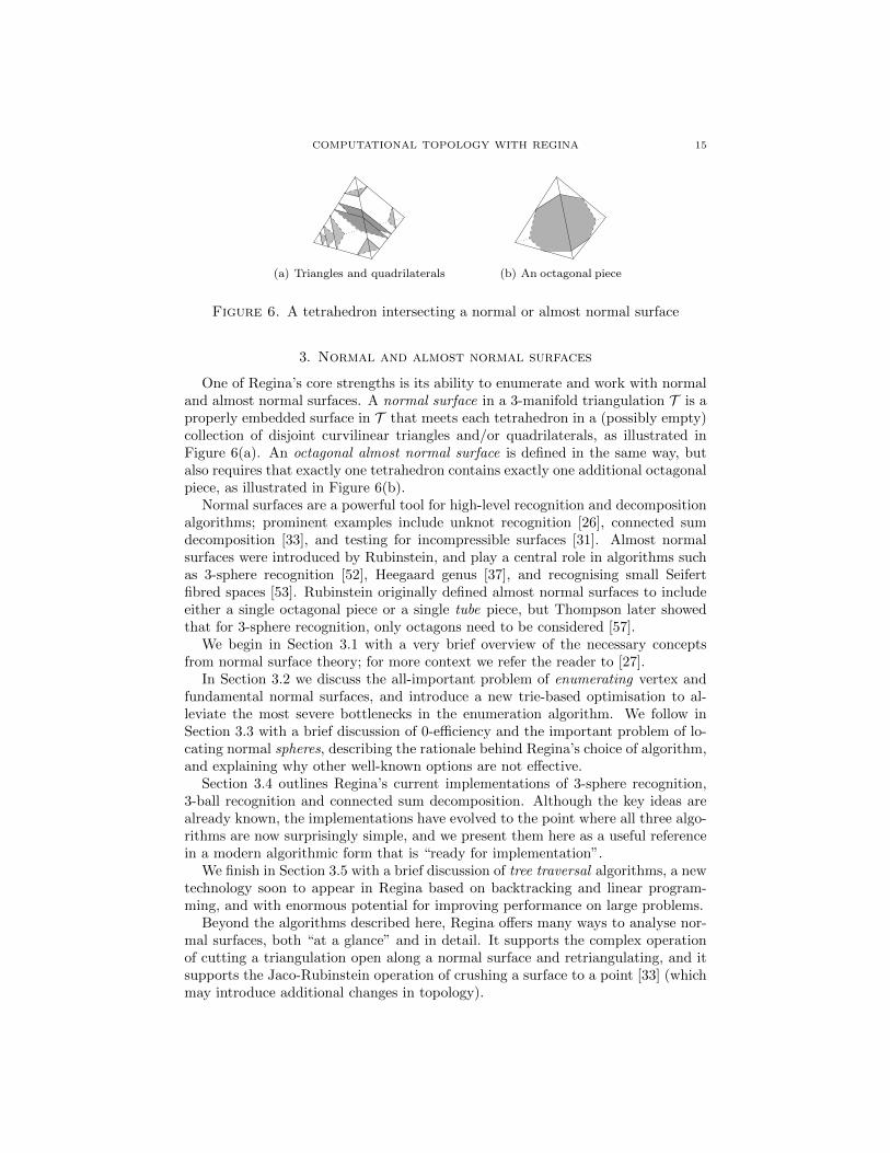
Figure 6. A tetrahedron intersecting a normal or almost normal surface
3. Normal and almost normal surfaces
One of Regina’s core strengths is its ability to enumerate and work with normaland almost normal surfaces. A normal surface in a 3-manifold triangulation T is aproperly embedded surface in T that meets each tetrahedron in a (possibly empty)collection of disjoint curvilinear triangles and/or quadrilaterals, as illustrated inFigure 6(a). An octagonal almost normal surface is defined in the same way, butalso requires that exactly one tetrahedron contains exactly one additional octagonalpiece, as illustrated in Figure 6(b).
Normal surfaces are a powerful tool for high-level recognition and decompositionalgorithms; prominent examples include unknot recognition [26], connected sumdecomposition [33], and testing for incompressible surfaces [31]. Almost normalsurfaces were introduced by Rubinstein, and play a central role in algorithms suchas 3-sphere recognition [52], Heegaard genus [37], and recognising small Seifertfibred spaces [53]. Rubinstein originally defined almost normal surfaces to includeeither a single octagonal piece or a single tube piece, but Thompson later showedthat for 3-sphere recognition, only octagons need to be considered [57].
We begin in Section 3.1 with a very brief overview of the necessary conceptsfrom normal surface theory; for more context we refer the reader to [27].
In Section 3.2 we discuss the all-important problem of enumerating vertex andfundamental normal surfaces, and introduce a new trie-based optimisation to al-leviate the most severe bottlenecks in the enumeration algorithm. We follow inSection 3.3 with a brief discussion of 0-efficiency and the important problem of lo-cating normal spheres, describing the rationale behind Regina’s choice of algorithm,and explaining why other well-known options are not effective.
Section 3.4 outlines Regina’s current implementations of 3-sphere recognition,3-ball recognition and connected sum decomposition. Although the key ideas arealready known, the implementations have evolved to the point where all three algo-rithms are now surprisingly simple, and we present them here as a useful referencein a modern algorithmic form that is “ready for implementation”.
We finish in Section 3.5 with a brief discussion of tree traversal algorithms, a newtechnology soon to appear in Regina based on backtracking and linear program-ming, and with enormous potential for improving performance on large problems.
Beyond the algorithms described here, Regina offers many ways to analyse nor-mal surfaces, both “at a glance” and in detail. It supports the complex operationof cutting a triangulation open along a normal surface and retriangulating, and itsupports the Jaco-Rubinstein operation of crushing a surface to a point [33] (whichmay introduce additional changes in topology).

16 BENJAMIN A. BURTON
3.1. Preliminaries from normal surface theory. In an n-tetrahedron trian-gulation T , normal surfaces correspond to integer vectors in a cone of the form{x ∈ R7n |Ax = 0, x ≥ 0}, where the matrix A of matching equations is de-rived from T . The 7n coordinates are grouped into 4n triangle coordinates, whichcount the triangles at each corner of each tetrahedron, and 3n quadrilateral coor-dinates, which count the quadrilaterals passing through each tetrahedron in eachof the three possible directions. Such vectors must also satisfy the quadrilateralconstraints, which require that at most one quadrilateral coordinate within eachtetrahedron can be non-zero. These constraints map out a (typically non-convex)union of faces of the cone above.
An important observation is that non-trivial connected normal surfaces can bereconstructed from their 3n quadrilateral coordinates alone [59]. We can thereforeidentify such surfaces with integer points in a smaller-dimensional cone of the form{x ∈ R3n |Bx = 0, x ≥ 0}. We refer to R7n and R3n as working in standardcoordinates and quadrilateral coordinates respectively.
A normal surface is called a (standard or quadrilateral) vertex surface if itsvector in (standard or quadrilateral) coordinates lies on an extreme ray of the cor-responding cone, and it is called a (standard or quadrilateral) fundamental surfaceif its vector lies in the Hilbert basis of the cone. The quadrilateral vertex andfundamental surfaces are typically a strict subset of their standard counterparts.
Throughout this paper, we use the phrase almost normal surface to refer ex-clusively to the case where the extra piece is an octagon (not a tube). For al-most normal surfaces we introduce three additional octagon coordinates for eachtetrahedron, yielding a cone in standard almost normal coordinates of the form{x ∈ R10n |Cx = 0, x ≥ 0}. As before, non-trivial connected surfaces can bereconstructed from their 3n quadrilateral and 3n octagon coordinates [9], yieldinga cone in quadrilateral-octagon coordinates of the form {x ∈ R6n |Dx = 0, x ≥ 0}.We can likewise define vertex and fundamental surfaces in these coordinate systems.
To finish, we make the well-known observation that Euler characteristic is alinear function in standard normal and almost normal coordinates [34], though itis not linear in quadrilateral or quadrilateral-octagon coordinates.
3.2. Enumeration. Many high-level algorithms are based on locating particularsurfaces, which—if they exist—can be found as vertex normal surfaces, or for somemore difficult algorithms, fundamental normal surfaces. Regina comes with heavilyoptimised algorithms for enumerating all vertex normal surfaces [8] or fundamentalnormal surfaces [13] in a triangulation, in all of the coordinate systems listed above.
Here we focus on the vertex enumeration algorithm, which is based on the doubledescription method for enumerating extreme rays of polyhedral cones [24, 47]. Weoutline the double description method very briefly, and then introduce a new trie-based optimisation that yields significant improvements in its running time.
In brief, the double description method enumerates the extreme rays of the cone{x ∈ Rd |Ax = 0, x ≥ 0} by constructing a series of cones C0, C1, . . ., where eachCi is defined only using the first i rows of A. The initial cone C0 is simply thenon-negative orthant, with extreme rays defined by the d unit vectors, and eachsubsequent cone Ci is obtained inductively from Ci−1 by intersecting with a newhyperplane Hi. The extreme rays of Ci are obtained from (i) extreme rays of Ci−1that lie on Hi; and (ii) convex combinations of pairs of adjacent extreme rays ofCi−1 that lie on either side of Hi.
COMPUTATIONAL TOPOLOGY WITH REGINA 17
· , · , ·
0, · , · +, · , ·
0,+, · +, 0, · +,+, ·
0, 2, 3 1, 0, 2 4, 1, 0 Extreme rays
Legend
· Unknown0 Zero+ Positive
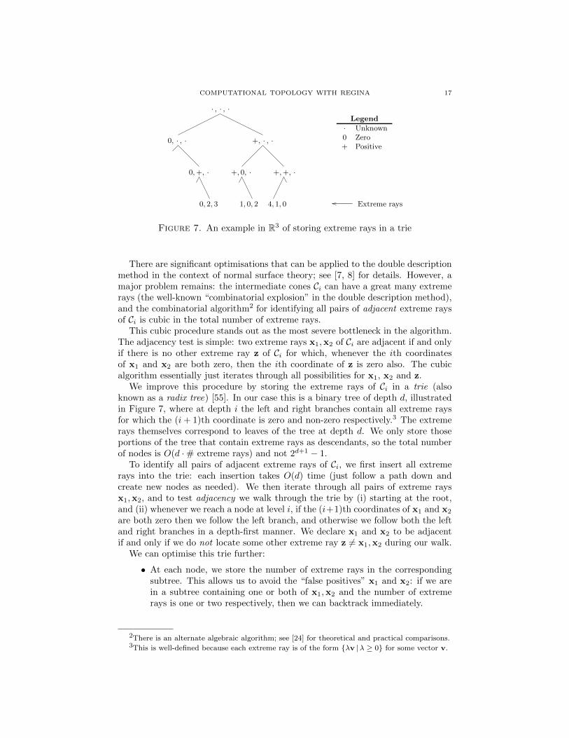
Figure 7. An example in R3 of storing extreme rays in a trie
There are significant optimisations that can be applied to the double descriptionmethod in the context of normal surface theory; see [7, 8] for details. However, amajor problem remains: the intermediate cones Ci can have a great many extremerays (the well-known “combinatorial explosion” in the double description method),and the combinatorial algorithm2 for identifying all pairs of adjacent extreme raysof Ci is cubic in the total number of extreme rays.
This cubic procedure stands out as the most severe bottleneck in the algorithm.The adjacency test is simple: two extreme rays x1,x2 of Ci are adjacent if and onlyif there is no other extreme ray z of Ci for which, whenever the ith coordinatesof x1 and x2 are both zero, then the ith coordinate of z is zero also. The cubicalgorithm essentially just iterates through all possibilities for x1, x2 and z.
We improve this procedure by storing the extreme rays of Ci in a trie (alsoknown as a radix tree) [55]. In our case this is a binary tree of depth d, illustratedin Figure 7, where at depth i the left and right branches contain all extreme raysfor which the (i+ 1)th coordinate is zero and non-zero respectively.3 The extremerays themselves correspond to leaves of the tree at depth d. We only store thoseportions of the tree that contain extreme rays as descendants, so the total numberof nodes is O(d ·# extreme rays) and not 2d+1 − 1.
To identify all pairs of adjacent extreme rays of Ci, we first insert all extremerays into the trie: each insertion takes O(d) time (just follow a path down andcreate new nodes as needed). We then iterate through all pairs of extreme raysx1,x2, and to test adjacency we walk through the trie by (i) starting at the root,and (ii) whenever we reach a node at level i, if the (i+1)th coordinates of x1 and x2
are both zero then we follow the left branch, and otherwise we follow both the leftand right branches in a depth-first manner. We declare x1 and x2 to be adjacentif and only if we do not locate some other extreme ray z 6= x1,x2 during our walk.
We can optimise this trie further:
• At each node, we store the number of extreme rays in the correspondingsubtree. This allows us to avoid the “false positives” x1 and x2: if we arein a subtree containing one or both of x1,x2 and the number of extremerays is one or two respectively, then we can backtrack immediately.
2There is an alternate algebraic algorithm; see [24] for theoretical and practical comparisons.3This is well-defined because each extreme ray is of the form {λv |λ ≥ 0} for some vector v.

18 BENJAMIN A. BURTON
Figure 8. Examples of collapsing non-tetrahedron pieces
• We can “compress” the trie by storing extreme rays at the nodes corre-sponding to their last non-zero coordinate, instead of at depth d, a usefuloptimisation given that our extreme rays may contain many zeroes.
The appeal of this data structure is that we are able to target our search by onlylooking at “promising” candidates for z, instead of scanning through all extremerays. It is difficult to pin down the theoretical complexity of our trie-based search;certainly it might be exponential in d (because of the branching), but it is clearlyno worse than O(d ·# extreme rays), i.e., the total number of nodes.
In practice, it serves us very well. Consider again the 23-tetrahedron triangu-lation of the Weber-Seifert dodecahedral space from [18]. With the original im-plementation of the double description method (including all optimisations exceptfor the trie-based search), enumerating all 698 quadrilateral vertex normal surfacesrequires 174 minutes (measured on a 2.93 GHz Intel Core i7). The new trie-basedalgorithm reduces this to 62 minutes, cutting the running time from roughly threehours down to just one.
3.3. 0-efficiency. An important problem in normal surface theory is searching fornormal spheres: this is at the heart of Jaco and Rubinstein’s 0-efficiency machinery[33], and features in all of the high-level algorithms listed in Section 3.4.
A closed orientable 3-manifold is 0-efficient if its only normal 2-spheres arethe trivial vertex linking spheres (which contain only triangles, and which mustalways be present). If a triangulation is not 0-efficient, then we can use Jaco andRubinstein’s “destructive crushing” procedure [33]: we crush the non-trivial sphereto a point, and then collapse away any degenerate non-tetrahedron pieces (such asfootballs, pillows and so on) to become edges and faces, as illustrated in Figure 8.
The result is that every tetrahedron that contains a quadrilateral from the non-trivial sphere will disappear entirely, and the final triangulation (which might bedisconnected) will be closed and have strictly fewer tetrahedra than the original.The crushing process might introduce topological changes, but these are limited topulling apart connected sums, adding new 3-sphere components, and deleting S3,RP 3, S2×S1 and/or L3,1 components. The crushing process is simple to implement(in stark contrast to the messy procedure of cutting along a normal surface), andwith help from first homology groups any topological changes are easy to detect.
In order to test for 0-efficiency (and to explicitly identify a non-trivial normalsphere if one exists), Regina uses the following result:
Lemma 3.1. If a closed orientable triangulation T contains a non-vertex-linkingnormal sphere, then it contains one as a quadrilateral vertex normal surface.
Proof. This result is widely known, but (to the author’s best knowledge) does notappear in the literature, and so we outline the simple proof here. When we convertto vectors in standard coordinates, any connected non-vertex-linking normal surfaceF can be expressed as a positive rational combination of one or more quadrilateral

COMPUTATIONAL TOPOLOGY WITH REGINA 19
Figure 9. Growth of the running time for the double description method
vertex normal surfaces, minus zero or more vertex linking spheres. Since the Eulercharacteristic χ is linear in standard coordinates and χ(S2) > 0, it follows that ifF is a non-trivial normal sphere then some quadrilateral vertex normal surface Qmust have χ(Q) > 0, whereupon some rational multiple of Q must be a non-trivialnormal sphere also. �
At present, Regina tests for 0-efficiency by enumerating all quadrilateral vertexnormal surfaces (up to multiples) and testing each. This of course is more workthan we need to do, since we only need to locate one non-trivial sphere. We outlinesome tempting alternatives now, and explain why Regina does not use them.
The first alternative is that, in standard coordinates, we could restrict our poly-hedral cone by adding the homogeneous linear constraint χ ≥ 0. This has beentried in Regina, but yields a substantially slower algorithm. Experimentation sug-gests that this is because (i) we are forced to work in the higher-dimensional R7n
instead of R3n; and (ii) the constraint χ ≥ 0 slices through the cone in a way thatcreates significantly more extreme rays, exacerbating the combinatorial explosionin the double description method.
The second alternative is based on linear programming. Casson and Jaco et al.[30] have suggested (in essence) that, for each of the 3n choices of which quadrilat-eral coordinate we allow to be non-zero in each tetrahedron, we could solve a linearprogram (in polynomial time) to maximise χ over a corresponding sub-cone in R7n.This is a promising approach, but it has a significant problem: for “good” trian-gulations, which typically are 0-efficient, we must attempt all 3n linear programsbefore we can terminate. That is, 3n becomes a lower bound on the running time.
Although the best known theoretical time complexity for a full vertex enumera-tion is slower than this [17], in practice a full enumeration is typically much faster.For example, when enumerating quadrilateral vertex normal surfaces for the first1000 triangulations in the Hodgson-Weeks closed hyperbolic census [29] (a goodsource of “difficult” manifolds for normal surface enumeration), the optimised dou-ble description method gives a running time that grows roughly like 1.6n, as shownin Figure 9.
20 BENJAMIN A. BURTON
3.4. High-level algorithms. Here we present Regina’s current implementationsof the high-level 3-sphere recognition, 3-ball recognition and connected sum decom-position algorithms. As noted earlier, the key ideas are already known; the purposeof this description is to give a useful reference for these algorithms in a modern“ready to implement” form.
It should be noted that all three algorithms guarantee both correctness and ter-mination (i.e., they are not probabilistic in nature). The 3-sphere recognition andconnected sum decomposition algorithms include developments from many authors[9, 32, 33, 34, 36, 52, 57], and the 3-ball recognition algorithm is a trivial modifi-cation of 3-sphere recognition. See [43] for a related but non-equivalent variant of3-sphere recognition based on special spines.
Algorithm 3.2 (3-sphere recognition). The following algorithm tests whether agiven triangulation T is a triangulation of the 3-sphere.
(1) Test whether T is closed, connected and orientable. If T fails any of thesetests, terminate and return false.
(2) Simplify T using Algorithm 2.5.(3) Test whether T has trivial homology. If not, terminate and return false.(4) Create a list L of triangulations to process, initially containing just T .
While L is non-empty:• Let N be the next triangulation in the list L. Remove N from L, and
test whether N has a quadrilateral vertex normal sphere F .– If so, then perform the Jaco-Rubinstein crushing procedure on F .
For each connected component N ′ of the resulting triangulation,simplify N ′ and add it back into the list L.
– If not, and if N has only one vertex, then search for a quadrila-teral-octagon vertex almost normal sphere in N . If none existsthen terminate and return false.
(5) Once there are no more triangulations in L, terminate and return true.
The key invariant in the algorithm above is that the original 3-manifold is alwaysthe connected sum of all manifolds in L. The homology test in step (3) is crucial,since the Jaco-Rubinstein crushing procedure could silently delete S2 × S1, RP 3
and/or L3,1 components.
Algorithm 3.3 (3-ball recognition). The following algorithm tests whether a giventriangulation T is a triangulation of the 3-ball.
(1) Test whether T is connected, orientable, has precisely one boundary com-ponent, and this boundary component is a 2-sphere. If T fails any of thesetests, terminate and return false.
(2) Simplify T using Algorithm 2.5.(3) Cone the boundary of T to a point by attaching one new tetrahedron to each
boundary face, and simplify again.(4) Run 3-sphere recognition over the final triangulation, and return the result.
For our final algorithm, we note that by “connected sum decomposition” we meana decomposition into non-trivial prime summands (i.e., no unwanted S3 terms).
Algorithm 3.4 (Connected sum decomposition). The following algorithm com-putes the connected sum decomposition of the manifold described by a given trian-gulation T . We assume as a precondition that T is closed, connected and orientable.
COMPUTATIONAL TOPOLOGY WITH REGINA 21
(1) Simplify T using Algorithm 2.5.(2) Compute the first homology of T , and let r, t2 and t3 denote the rank,
Z2 rank and Z3 rank respectively.(3) Create an input list L of triangulations to process, initially containing justT , and an output list O of prime summands, initially empty.While L is non-empty:• Let N be the next triangulation in the list L. Remove N from L, and
test whether N has a quadrilateral vertex normal sphere F .– If so, then perform the Jaco-Rubinstein crushing procedure on F .
For each connected component N ′ of the resulting triangulation,simplify N ′ and add it back into the list L.
– If not, then append N to the output list O if either (i) N hasnon-trivial homology, or (ii) N has only one vertex and no quad-rilateral-octagon vertex almost normal sphere.
(4) Compute the first homology of each triangulation in the output list O, sumthe ranks, Z2 ranks and Z3 ranks, and append additional copies of S2×S1,RP 3 and L3,1 to O so that these ranks sum to r, t2 and t3 respectively.
On termination, the output list O will contain triangulations of the (non-trivial)prime summands of the input manifold.
The key invariants of this algorithm are that (i) the input manifold is always theconnected sum of all manifolds in L and O, plus zero or more S2×S1, RP 3 and/orL3,1 summands; and that (ii) every output manifold in O is prime and not S3.
3.5. Tree traversal algorithms. There have been recent interesting develop-ments in computational normal surface theory that could allow us to move awayfrom the double description method entirely. These are algorithms based on travers-ing a search tree [17, 16], and they combine aspects of linear programming, polytopetheory and data structures.
The resulting algorithms avoid the dreaded combinatorial explosion of the doubledescription method; moreover, they offer incremental output and are well-suited toparallelisation, progress tracking and early termination. Most importantly, experi-mentation suggests that they are significantly faster and less memory-hungry—evenwhen run in serial—for larger and more difficult problems. The code is already upand running, and will be included in the next release of Regina.
Such tree traversal algorithms can be used for either a full enumeration of vertexnormal surfaces [17], or to locate a single non-trivial normal or almost normal sphere(for 0-efficiency testing and/or 3-sphere recognition) [16]. The key idea is to builda search tree according to which quadrilateral coordinates are non-zero in eachtetrahedron, and to run incremental linear programs that enforce the quadrilateralconstraints for those tetrahedra where decisions have been made, but ignore thequadrilateral constraints for those tetrahedra that we have not yet processed.
For the full enumeration of vertex normal surfaces, details of the tree traversalalgorithm can be found in [17]. To illustrate, we return again to the 23-tetrahedrontriangulation of the Weber-Seifert dodecahedral space: whereas the trie-based dou-ble description method enumerates all 698 quadrilateral vertex normal surfaces in62 minutes, the tree traversal algorithm does this in just 32 minutes.
For locating just a single normal or almost normal sphere, the tree traversalalgorithm becomes extremely powerful: it can prove that this same triangulation of
22 BENJAMIN A. BURTON
the Weber-Seifert dodecahedral space is 0-efficient in under 10 seconds. Note thatthere is no early termination here—the tree traversal algorithm conclusively provesin under 10 seconds that no non-trivial normal sphere exists.
This latter algorithm for locating normal and almost normal spheres relies on anumber of crucial heuristics, and full details can be found in [16]. Perhaps mostinteresting is the following experimental observation: for “typical” inputs, thisalgorithm appears to require only a linear number of linear programs; that is, thetypical behaviour appears to be polynomial-time. One should be quick to note thatthis is in experimentation only, and that the algorithm is not polynomial-time inthe worst case. Nevertheless, this is a very exciting computational development.
4. Combinatorial recognition
In this brief section we outline Regina’s combinatorial recognition code. Despitesignificant advances in 3-manifold algorithms, we as a community are still a longway from being able to implement the full homeomorphism algorithm—even simplerproblems such as JSJ decomposition have never been implemented, and Hakennesstesting (which plays a key role in the homeomorphism problem) has only recentlybecome practical [18]. These are the issues that we aim to address (or rather workaround) here.
In addition to slower but always-correct and always-conclusive algorithms such as3-sphere recognition and connected sum decomposition, Regina offers a secondarymeans for identifying 3-manifolds: combinatorial recognition. The central idea isthat we “hard-code” a large number of general constructions for infinite families of3-manifolds (such as Seifert fibred spaces, surface bundles and graph manifolds).Then, given an input triangulation T , we test whether T follows one of these hard-coded constructions, and if it does, we “read off” the parameters to name theunderlying 3-manifold.
The advantages of this technique are:
• It is extremely fast—all of Regina’s hard-coded constructions of infinitefamilies can be recognised in small polynomial time.• It allows Regina to recognise a much larger range of 3-manifolds than would
otherwise be practically possible.
There are, of course, clear disadvantages:
• Such techniques require a lot of code if we wish to recognise each construc-tion in its full generality: Regina currently has over 25 000 lines of sourcecode devoted to combinatorial recognition alone.• The code is only as powerful and general as the constructions that are im-
plemented. For instance, with a handful of exceptions, Regina’s recognitionroutines do not include any hyperbolic manifolds.• To be recognised, a triangulation must be well-structured—an arbitrary
triangulation of even a simple manifold such as a lens space will not berecognised unless it follows one of the known constructions.
Despite these drawbacks, combinatorial recognition is enormously useful in prac-tice. Regina’s recognition code is particularly strong for non-orientable manifolds:of the 366 manifolds in the ≤ 11-tetrahedron closed non-orientable census [10],Regina is able to recognise all minimal triangulations for 334 of them, and is ableto recognise at least one minimal triangulation for 357—that is, all but nine.

COMPUTATIONAL TOPOLOGY WITH REGINA 23
α
αβ
β
γγ
2α+ 2β + 2γ = 2π
∑angles = 2π
Figure 10. The conditions for an angle structure on a triangulation
If Regina cannot recognise the manifold from an input triangulation T (i.e., thecombinatorial recognition is inconclusive), then often a good strategy is to modifyT so that the triangulation becomes more “well-structured”. This might include(i) simplifying T using Algorithm 2.5, or (ii) the slower but stronger technique ofperforming a breadth-first from T through Pachner graph until we reach a trian-gulation that can be recognised, following the discussion in Section 2.5.
Regina is not the only software package to employ combinatorial recognition:there is also the 3-Manifold Recogniser by Matveev et al., which has extremelypowerful recognition heuristics that can recognise a much wider range of 3-manifoldsthan Regina can. See [43, 44, 45] for details.
5. Angle structures
In addition to normal surfaces, Regina can also enumerate and analyse anglestructures on a triangulation T . An angle structure assigns non-negative internaldihedral angles to each edge of each tetrahedron of T , so that (i) opposite edges of atetrahedron are assigned the same angle; (ii) all angles in a tetrahedron sum to 2π;and (iii) all angles around any internal edge of T likewise sum to 2π (see Figure 10).Such structures are often called semi-angle structures [35], to distinguish them fromstrict angle structures in which all angles are strictly positive. Note that, by a simpleEuler characteristic computation, an angle structure can only exist if T is an idealtriangulation with every vertex link a torus or Klein bottle.
Angle structures were introduced by Rivin [50, 51] and Casson, with furtherdevelopment by Lackenby [38], and are a simpler (but weaker) combinatorial ana-logue of a complete hyperbolic structure. Some angle structures are of particularinterest: these include taut angle structures4 in which every angle is precisely 0 orπ (representing “flattened” tetrahedra) [28, 39], and veering structures which aretaut angle structures with powerful combinatorial constraints [1, 28]. All of theseobjects have an interesting role to play in building a complete hyperbolic structureon T [25, 28, 35].
Conditions (i)–(iii) above map out a polytope in R3n, where n is the numberof tetrahedra; the vertices of this polytope are called vertex angle structures, andtheir convex combinations generate all possible angle structures on T . For manyyears now, Regina has been able to enumerate all vertex angle structures using thedouble description method, as outlined in Section 3.2. Moreover, it can detect tautangle structures and (more recently) veering structures when they are present.
A newer development is that Regina can enumerate only taut angle structures.Detecting even a single taut angle structure is NP-complete [19]; nevertheless,
4We follow the nomenclature of Hodgson et al. [28]—these are slightly more general than theoriginal taut structures of Lackenby [39], who also adds a coorientation constraint.

24 BENJAMIN A. BURTON
Regina can enumerate all taut angle structures for relatively large triangulations—in ad-hoc experiments it can do this for 70–80 tetrahedra in a matter of minutes.
The underlying algorithm is based on the following simple observation:
Lemma 5.1. Every taut angle structure is also a vertex angle structure.
Proof. Describing angle structures by vectors in R3n as outlined above, supposethat τ = λα1 + (1− λ)α2 where λ ∈ (0, 1), and where τ, α1, α2 are angle structureswith τ taut. Then both α1 and α2 must have dihedral angles of zero wherever τhas a dihedral angle of zero, whereupon it follows that α1 = α2 = τ . �
Algorithm 5.2. Given an n-tetrahedron triangulation T , the following algorithmenumerates all taut angle structures on T .
First, we projectivise the polytope described by conditions (i)–(iii) above. This isa standard construction: we add a (3n+1)th coordinate, embed the original polytopeP in the hyperplane x3n+1 = 1, and build the cone from the origin through P. Thisreplaces our bounded polytope P ⊆ R3n with a polyhedral cone C ⊆ R3n+1 of theform C = {x ∈ R3n+1 |Ax = 0, x ≥ 0}. The vertex angle structures in the originalpolytope P now correspond to the extreme rays of the cone C.
We run the double description method to enumerate all extreme rays of C. Recallthat this inductively constructs cones C0, C1, . . ., where Ci is obtained from Ci−1 byintersecting with a new hyperplane Hi, and where each extreme ray of Ci is either(a) an extreme ray of Ci−1 that lies on Hi, or (b) the convex combination of twoadjacent extreme rays x1,x2 of Ci−1 that lie on opposite sides of Hi.
Here we introduce a simple but crucial optimisation: in case (b) above, we onlyconsider pairs x1,x2 that together do not have positive values in more than onecoordinate position per tetrahedron.
This optimisation is similar to Letscher’s filtering method for normal surfaceenumeration [8]. It works because, if some pair x1,x2 fails the final conditionabove, then (by virtue of the fact that all angles are non-negative and we alwaysperform convex combinations) any vertex angle structure that we eventually obtainfrom a combination of x1 and x2 must have multiple non-zero coordinates in sometetrahedron, and so cannot be taut.
Finally, we note that we can improve the enumeration algorithm further, bothfor enumerating taut angle structures and enumerating all vertex angle structures,by employing the same trie-based optimisation that we introduce in Section 3.2.
6. Experimentation
In this penultimate section we illustrate how Regina can be used for both small-scale and large-scale experimentation, in the hope that readers can use this as atemplate for beginning their own experiments.
In addition to its graphical user interface, Regina offers a powerful scripting fa-cility, in which most of the C++ classes and functions in its mathematical engine aremade available through a dedicated Python module. Python is a popular scriptinglanguage that is easy to write and easy to read, and the Python module in Reginamakes it easy to quickly prototype new algorithms, run tests over large bodiesof census data, or perform complex tasks that would be cumbersome through apoint-and-click interface.
Users can access Regina’s Python module in two ways:

COMPUTATIONAL TOPOLOGY WITH REGINA 25
• by opening a Python console from within the graphical user interface, whichallows users to study or modify data in the current working file;• by starting the command-line program regina-python, which brings up a
standalone Python prompt.
Users can also run their own Python scripts directly via regina-python, embedscripts within data files as script packets, or write their own libraries of frequently-used routines that will be loaded automatically each time a Regina Python sessionstarts.
The following sample Python session constructs the triangulation of RP 3 thatwas illustrated in Section 2.1, prints its first homology group, enumerates all vertexnormal surfaces, and then locates and prints the coordinates of the vectors thatrepresent vertex normal projective planes.
bab@rosemary:~$ regina-python
Regina 4.93
Software for 3-manifold topology and normal surface theory
Copyright (c) 1999-2012, The Regina development team
>>> tri = NTriangulation()
>>> t0 = tri.newTetrahedron()
>>> t1 = tri.newTetrahedron()
>>> t0.joinTo(0, t1, NPerm4(1,0,3,2)) # Glues 0 (123) -> 1 (032)
>>> t0.joinTo(1, t1, NPerm4(1,0,3,2)) # Glues 0 (023) -> 1 (132)
>>> t0.joinTo(2, t1, NPerm4(0,1,2,3)) # Glues 0 (013) -> 1 (013)
>>> t0.joinTo(3, t1, NPerm4(0,1,2,3)) # Glues 0 (012) -> 1 (012)
>>> print tri.getHomologyH1()
Z_2
>>> s = NNormalSurfaceList.enumerate(tri, NNormalSurfaceList.STANDARD, 1)
>>> print s
5 vertex normal surfaces (Standard normal (tri-quad))
>>> for i in range(s.getNumberOfSurfaces()):
... if s.getSurface(i).getEulerCharacteristic() == 1:
... print s.getSurface(i)
...
0 0 0 0 ; 0 1 0 || 0 0 0 0 ; 0 1 0
0 0 0 0 ; 0 0 1 || 0 0 0 0 ; 0 0 1
>>>
One of Regina’s most useful facilities for experimentation is its ability to createcensus data: exhaustive lists of all 3-manifold triangulations (up to combinatorialisomorphism) that satisfy some given set of constraints. The census algorithms areheavily optimised [4, 6, 10], and can be run in serial on a desktop or in parallel ona large supercomputer.
The simplest way for users to create their own census data is through thecommand-line tricensus tool. The following example constructs all 532 closedorientable 3-manifold triangulations with n = 4 tetrahedra:
bab@rosemary:~$ tricensus --tetrahedra=4 --internal --orientable --finite
--sigs output.txt
Starting census generation...
0:1 0:0 1:0 1:1 | 0:2 0:3 2:0 2:1 | 1:2 1:3 3:0 3:1 | 2:2 2:3 3:3 3:2
0:1 0:0 1:0 1:1 | 0:2 0:3 2:0 3:0 | 1:2 2:2 2:1 3:1 | 1:3 2:3 3:3 3:2
0:1 0:0 1:0 1:1 | 0:2 0:3 2:0 3:0 | 1:2 3:1 3:2 3:3 | 1:3 2:1 2:2 2:3
0:1 0:0 1:0 2:0 | 0:2 1:2 1:1 3:0 | 0:3 2:2 2:1 3:1 | 1:3 2:3 3:3 3:2
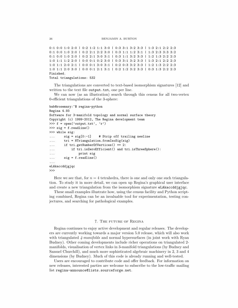
26 BENJAMIN A. BURTON
0:1 0:0 1:0 2:0 | 0:2 1:2 1:1 3:0 | 0:3 3:1 3:2 3:3 | 1:3 2:1 2:2 2:3
0:1 0:0 1:0 2:0 | 0:2 2:1 2:2 3:0 | 0:3 1:1 1:2 3:1 | 1:3 2:3 3:3 3:2
0:1 0:0 1:0 2:0 | 0:2 2:1 3:0 3:1 | 0:3 1:1 3:2 3:3 | 1:2 1:3 2:2 2:3
1:0 1:1 1:2 2:0 | 0:0 0:1 0:2 3:0 | 0:3 3:1 3:2 3:3 | 1:3 2:1 2:2 2:3
1:0 1:1 2:0 2:1 | 0:0 0:1 3:0 3:1 | 0:2 0:3 3:2 3:3 | 1:2 1:3 2:2 2:3
1:0 1:1 2:0 3:0 | 0:0 0:1 2:1 3:1 | 0:2 1:2 3:2 3:3 | 0:3 1:3 2:2 2:3
Finished.
Total triangulations: 532
The triangulations are converted to text-based isomorphism signatures [12] andwritten to the text file output.txt, one per line.
We can now (as an illustration) search through this census for all two-vertex0-efficient triangulations of the 3-sphere:
bab@rosemary:~$ regina-python
Regina 4.93
Software for 3-manifold topology and normal surface theory
Copyright (c) 1999-2012, The Regina development team
>>> f = open(’output.txt’, ’r’)
>>> sig = f.readline()
>>> while sig:
... sig = sig[0:-1] # Strip off trailing newline
... tri = NTriangulation.fromIsoSig(sig)
... if tri.getNumberOfVertices() == 2:
... if tri.isZeroEfficient() and tri.isThreeSphere():
... print sig
... sig = f.readline()
...
eLAkaccddjgjqc
>>>
Here we see that, for n = 4 tetrahedra, there is one and only one such triangula-tion. To study it in more detail, we can open up Regina’s graphical user interfaceand create a new triangulation from the isomorphism signature eLAkaccddjgjqc.
These small examples illustrate how, using the census facility and Python script-ing combined, Regina can be an invaluable tool for experimentation, testing con-jectures, and searching for pathological examples.
7. The future of Regina
Regina continues to enjoy active development and regular releases. The develop-ers are currently working towards a major version 5.0 release, which will also workwith triangulated 4-manifolds and normal hypersurfaces (in joint work with RyanBudney). Other coming developments include richer operations on triangulated 2-manifolds, visualisation of vertex links in 3-manifold triangulations (by Budney andSamuel Churchill), and much more sophisticated algebraic machinery in 2, 3 and 4dimensions (by Budney). Much of this code is already running and well-tested.
Users are encouraged to contribute code and offer feedback. For information onnew releases, interested parties are welcome to subscribe to the low-traffic mailinglist [email protected].

COMPUTATIONAL TOPOLOGY WITH REGINA 27
References
1. Ian Agol, Ideal triangulations of pseudo-Anosov mapping tori, Topology and Geometry inDimension Three, Contemp. Math., vol. 560, Amer. Math. Soc., Providence, RI, 2011, pp. 1–
17.
2. Bruno Benedetti and Gunter M. Ziegler, On locally constructible spheres and balls, Acta Math.206 (2011), no. 2, 205–243.
3. Winfried Bruns and Bogdan Ichim, Normaliz: Algorithms for affine monoids and rational
cones, J. Algebra 324 (2010), no. 5, 1098–1113.4. Benjamin A. Burton, Face pairing graphs and 3-manifold enumeration, J. Knot Theory Ram-
ifications 13 (2004), no. 8, 1057–1101.5. , Introducing Regina, the 3-manifold topology software, Experiment. Math. 13 (2004),
no. 3, 267–272.
6. , Enumeration of non-orientable 3-manifolds using face-pairing graphs and union-find,Discrete Comput. Geom. 38 (2007), no. 3, 527–571.
7. , Converting between quadrilateral and standard solution sets in normal surface theory,
Algebr. Geom. Topol. 9 (2009), no. 4, 2121–2174.8. , Optimizing the double description method for normal surface enumeration, Math.
Comp. 79 (2010), no. 269, 453–484.
9. , Quadrilateral-octagon coordinates for almost normal surfaces, Experiment. Math. 19(2010), no. 3, 285–315.
10. , Detecting genus in vertex links for the fast enumeration of 3-manifold triangulations,ISSAC 2011: Proceedings of the 36th International Symposium on Symbolic and Algebraic
Computation, ACM, 2011, pp. 59–66.
11. , The Pachner graph and the simplification of 3-sphere triangulations, SCG ’11: Pro-ceedings of the Twenty-Seventh Annual Symposium on Computational Geometry, ACM, 2011,
pp. 153–162.
12. , Simplification paths in the Pachner graphs of closed orientable 3-manifold triangu-lations, Preprint, arXiv:1110.6080, October 2011.
13. , Enumerating fundamental normal surfaces: Algorithms, experiments and invariants,
ALENEX 2014: Proceedings of the Sixteenth Workshop on Algorithm Engineering and Ex-periments, SIAM, 2014, pp. 112–124.
14. Benjamin A. Burton, Ryan Budney, William Pettersson, et al., Regina: Software for 3-
manifold topology and normal surface theory, http://regina.sourceforge.net/, 1999–2012.15. Benjamin A. Burton and Melih Ozlen, Computing the crosscap number of a knot using integer
programming and normal surfaces, ACM Trans. Math. Software 39 (2012), no. 1, 4:1–4:18.16. , A fast branching algorithm for unknot recognition with experimental polynomial-time
behaviour, Preprint, arXiv:1211.1079, November 2012.
17. , A tree traversal algorithm for decision problems in knot theory and 3-manifold topol-ogy, Algorithmica 65 (2013), no. 4, 772–801.
18. Benjamin A. Burton, J. Hyam Rubinstein, and Stephan Tillmann, The Weber-Seifert dodec-
ahedral space is non-Haken, Trans. Amer. Math. Soc. 364 (2012), no. 2, 911–932.19. Benjamin A. Burton and Jonathan Spreer, The complexity of detecting taut angle structures
on triangulations, SODA ’13: Proceedings of the Twenty-Fourth Annual ACM-SIAM Sym-
posium on Discrete Algorithms, SIAM, 2013, pp. 168–183.20. Patrick J. Callahan, Martin V. Hildebrand, and Jeffrey R. Weeks, A census of cusped hyper-
bolic 3-manifolds, Math. Comp. 68 (1999), no. 225, 321–332.
21. Maurice Chiodo, Finding non-trivial elements and splittings in groups, J. Algebra 331 (2011),271–284.
22. Thomas H. Cormen, Charles E. Leiserson, Ronald L. Rivest, and Clifford Stein, Introductionto algorithms, 2nd ed., MIT Press, Cambridge, MA, 2001.
23. Marc Culler, Nathan M. Dunfield, and Jeffrey R. Weeks, SnapPy, a computer program forstudying the geometry and topology of 3-manifolds, http://snappy.computop.org/, 1991–2011.
24. Komei Fukuda and Alain Prodon, Double description method revisited, Combinatorics and
Computer Science (Brest, 1995), Lecture Notes in Comput. Sci., vol. 1120, Springer, Berlin,1996, pp. 91–111.

28 BENJAMIN A. BURTON
25. David Futer and Francois Gueritaud, From angled triangulations to hyperbolic structures, In-
teractions Between Hyperbolic Geometry, Quantum Topology and Number Theory, Contemp.
Math., vol. 541, Amer. Math. Soc., Providence, RI, 2011, pp. 159–182.26. Wolfgang Haken, Theorie der Normalflachen, Acta Math. 105 (1961), 245–375.
27. Joel Hass, Jeffrey C. Lagarias, and Nicholas Pippenger, The computational complexity of knot
and link problems, J. Assoc. Comput. Mach. 46 (1999), no. 2, 185–211.28. Craig D. Hodgson, J. Hyam Rubinstein, Henry Segerman, and Stephan Tillmann, Veering
triangulations admit strict angle structures, Geom. Topol. 15 (2011), no. 4, 2073–2089.
29. Craig D. Hodgson and Jeffrey R. Weeks, Symmetries, isometries and length spectra of closedhyperbolic three-manifolds, Experiment. Math. 3 (1994), no. 4, 261–274.
30. William Jaco, David Letscher, and J. Hyam Rubinstein, Algorithms for essential surfaces in 3-
manifolds, Topology and Geometry: Commemorating SISTAG, Contemporary Mathematics,no. 314, Amer. Math. Soc., Providence, RI, 2002, pp. 107–124.
31. William Jaco and Ulrich Oertel, An algorithm to decide if a 3-manifold is a Haken manifold,Topology 23 (1984), no. 2, 195–209.
32. William Jaco and J. Hyam Rubinstein, PL equivariant surgery and invariant decompositions
of 3-manifolds, Adv. Math. 73 (1989), no. 2, 149–191.33. , 0-efficient triangulations of 3-manifolds, J. Differential Geom. 65 (2003), no. 1, 61–
168.
34. William Jaco and Jeffrey L. Tollefson, Algorithms for the complete decomposition of a closed3-manifold, Illinois J. Math. 39 (1995), no. 3, 358–406.
35. Ensil Kang and J. Hyam Rubinstein, Ideal triangulations of 3-manifolds II; Taut and angle
structures, Algebr. Geom. Topol. 5 (2005), 1505–1533.36. Hellmuth Kneser, Geschlossene Flachen in dreidimensionalen Mannigfaltigkeiten, Jahres-
bericht der Deut. Math. Verein. 38 (1929), 248–260.37. Marc Lackenby, An algorithm to determine the Heegaard genus of simple 3-manifolds with
nonempty boundary, Algebr. Geom. Topol. 8 (2008), no. 2, 911–934.
38. , Word hyperbolic Dehn surgery, Invent. Math. 140 (2000), no. 2, 243–282.39. , Taut ideal triangulations of 3-manifolds, Geom. Topol. 4 (2000), 369–395.
40. A. A. Markov, Insolubility of the problem of homeomorphy, Proc. Internat. Congress Math.
1958, Cambridge Univ. Press, New York, 1960, pp. 300–306.41. Bruno Martelli and Carlo Petronio, Three-manifolds having complexity at most 9, Experiment.
Math. 10 (2001), no. 2, 207–236.
42. S. V. Matveev, Transformations of special spines, and the Zeeman conjecture, Izv. Akad.Nauk SSSR Ser. Mat. 51 (1987), no. 5, 1104–1116, 1119.
43. Sergei Matveev, Algorithmic topology and classification of 3-manifolds, Algorithms and Com-
putation in Mathematics, no. 9, Springer, Berlin, 2003.44. , 3-Manifold Recognizer and 3-Manifold Atlas, Oberwolfach Rep. 9 (2012), no. 2,
1409–1410.45. Sergei Matveev et al., Manifold recognizer, http://www.matlas.math.csu.ru/?page=
recognizer, accessed August 2012.
46. Sergei V. Matveev, Complexity theory of three-dimensional manifolds, Acta Appl. Math. 19(1990), no. 2, 101–130.
47. T. S. Motzkin, H. Raiffa, G. L. Thompson, and R. M. Thrall, The double description method,Contributions to the Theory of Games, Vol. II (H. W. Kuhn and A. W. Tucker, eds.), Annalsof Mathematics Studies, no. 28, Princeton University Press, Princeton, NJ, 1953, pp. 51–73.
48. Nokia Corporation, Qt – cross-platform application and UI framework, http://qt.nokia.
com/, 1992–2012.49. Udo Pachner, P.L. homeomorphic manifolds are equivalent by elementary shellings, European
J. Combin. 12 (1991), no. 2, 129–145.50. Igor Rivin, Euclidean structures on simplicial surfaces and hyperbolic volume, Ann. of Math.
(2) 139 (1994), no. 3, 553–580.
51. , Combinatorial optimization in geometry, Adv. in Appl. Math. 31 (2003), no. 1,242–271.
52. J. Hyam Rubinstein, An algorithm to recognize the 3-sphere, Proceedings of the International
Congress of Mathematicians (Zurich, 1994), vol. 1, Birkhauser, 1995, pp. 601–611.53. , An algorithm to recognise small Seifert fiber spaces, Turkish J. Math. 28 (2004),
no. 1, 75–87.

COMPUTATIONAL TOPOLOGY WITH REGINA 29
54. Peter Scott, The geometries of 3-manifolds, Bull. London Math. Soc. 15 (1983), no. 5, 401–
487.
55. Robert Sedgewick, Algorithms in C++, Addison-Wesley, Reading, MA, 1992.56. Robert Endre Tarjan, Efficiency of a good but not linear set union algorithm, J. ACM 22
(1975), no. 2, 215–225.
57. Abigail Thompson, Thin position and the recognition problem for S3, Math. Res. Lett. 1(1994), no. 5, 613–630.
58. William P. Thurston, The geometry and topology of 3-manifolds, Lecture notes, Princeton
University, 1978.59. Jeffrey L. Tollefson, Normal surface Q-theory, Pacific J. Math. 183 (1998), no. 2, 359–374.
60. Jeffrey R. Weeks, SnapPea: Hyperbolic 3-manifold software, http://www.geometrygames.org/
SnapPea/, 1991–2000.
School of Mathematics and Physics, The University of Queensland, Brisbane QLD
4072, Australia
E-mail address: [email protected]