Computational techniques in animal breeding

Computational techniques in

animal breeding

by

Ignacy Misztal

University of Georgia

Athens, USA

First Edition Sept 1999

Last Updated May 1, 2018

2

Contents

Preface ………………………………………………………………………………….. 5

Software engineering …………………………………………………………………… 7

Fortran ………………………………………………………………………………….. 9

Fortran 90 - Basics 10

Compiling 22

Advanced features in Fortran 95 24

General philosophy of Fortran 90 34

Fortran 2003 42

Parallel programming and OpenMP 44

Rewriting programs in F77 to F95 48

Setting-up mixed model equations ……………………………………………………. 51

Fixed 2-way model 51

Extension to more than two effects 53

Computer program 55

Model with covariables 57

Nested covariable 58

Computer program 60

Multiple trait least squares 62

Missing traits 65

Different models per trait 66

Example of ordering by models and by traits 66

Computer program 68

Mixed models 72

Popular contributions to random effects - single trait 72

Numerator relationship matrix A 73

Rules to create A-1 directly 74

Unknown parent groups 75

Numerator relationship matrix in the sire model 75

Variance ratios 77

Covariances between effects 79

Random effects in multiple traits 79

Multiple traits and correlated effects 80

Computer pseudo-code 81

Computer program 82

Storing and Solving Mixed Model Equations ………………………………………… 86

Storage of sparse matrices 87

Ordered or unordered triples 87

IJA 87

Linked lists 88

3

Trees 89

Summing MME 89

Searching algorithms 91

Numerical methods to solve a linear system of equations 93

Gaussian elimination 93

LU decomposition (Cholesky factorization) 94

Storage 96

Triangular 96

Sparse 96

Sparse matrix inversion 98

Numerical accuracy 99

Iterative methods 100

Jacobi 101

Gauss-Seidel and SOR 101

Preconditioned conjugate gradient 102

Other methods 103

Convergence properties of iterative methods 104

Properties of the Jacobi iteration 108

Properties of the Gauss-Seidel and SOR iterations 109

Practical convergence issues 109

Determination of best iteration parameters 109

Strategies for iterative solutions 110

Solving by effects 110

Iteration on data (matrix-free iteration) 110

Indirect representation of mixed-model equations 112

Summary of iteration strategies 117

Variance components …………………………………………………………………. 118

REML 118

General Properties of Maximization Algorithms 123

Some popular maximization algorithms 125

Acceleration to EM (fixed point) estimates 127

Convergence properties of maximization algorithms in REML 130

Accuracy of the D and DF algorithms 132

Method R 134

Bayesian methods and Gibbs sampling 139

Using the Gibbs sampler 144

Multiple-traits 146

Convergence properties 147

Ways to reduce the cost of multiple traits …………………………………………….. 150

Canonical transformation 150

Canonical transformation and REML 150

Numerical properties of canonical transformation 153

Extensions in canonical transformation 154

4

Multiple random effects 154

Missing traits 155

Different models per trait 155

Implicit representation of general multiple-trait equations 157

Computing in genomic selection ……………………………………………………… 161

Joint relationship matrix H and single-step GBLUP 163

Fine tuning 165

Large number of genotypes and APY algorithm 165

Data manipulation …………………………………………………………………….. 167

Renumbering 167

Memory consideration 167

Look-up tables 168

Sort and merge 169

Tools for data manipulation 175

Unix/Linux/MacOS utilities 176

Sources and References ……………………………………………………………….. 179

5

Preface

These notes originated as class notes for a graduate-level course taught at the University of

Georgia in 1997. The goal of that course was to train students to program new ideas in animal

breeding. Programming was in Fortran because Fortran programs are relatively easy for

numerical problems, and many existing packages in animal breeding still useful at that time were

written in Fortran. Since the computer science department at UGA does not teach courses in

Fortran any longer, the first few lectures were devoted to Fortran 77 and then to Fortran 90. All

programming examples and assignments were in Fortran 90. Because the students had only

limited experience in programming, the emphasis was on generality and simplicity even at some

loss of efficiency.

Programming examples from the course led to an idea of a general yet simple BLUP program

that can be easily modified to test new methodologies in animal breeding. An integral part of that

program was a sparse matrix module that allowed for easy but efficient programming of sparse

matrix computations.

The resulting program was called BLUPF90 and supported general multiple trait models with

missing traits, different models per trait, random regressions, separate pedigree files and

dominance. An addition of a subroutine plus a minor change in the main program converted

BLUPF90 to REMLF90 - an accelerated EM variance-component program, and BLUP90THR -

a bivariate threshold-linear model. An addition of subroutines created a Gibbs sampling program

GIBBSF90. I greatly appreciate collaborators who contributed to the project. Tomasz Strabel

added a dense-matrix library. Shogo Tsuruta created extensions of in-memory program to

iteration-on-data. Benoit Auvray added estimation of thresholds to the threshold model

programs. Monchai Duanginda, Olga Ravagnolo, and Deuhwan Lee worked on adding threshold

and threshold-linear model capability to GIBBSF90. Shogo Tsuruta and Tom Druet worked on

extension to AI-REML. Tom Druet wrote an extension to Method R, which can work with large

data sets.... Indirect contributions were made by Andres Legarra and Miguel Perez-Enciso. Many

contributions have been made by Ignacio Aguilar, whose goal was to speed the programs for

random regression models and adapt them for genomic selection. Yutaka Masuda added a sparse

package that makes calculations with sparse matrices much faster when they contain dense

blocks, as with genomic data, and updates the programs for large genomic data (including

implementation of the APY algorithm). Daniela Lourenco did extensive testing and helped with

the documentation.

Program development of BLUPF90 and the other programs was not painless. Almost every f90

compiler had bugs, and there were many small bugs in the programs. As Edison wrote, "the

success is 1% inspiration and 99 perspiration". Now the programs have been used for hundreds

of papers and are routinely applied for commercial genetic evaluations in many species.

However, there is always room for improvements.

The programming work took time away from the notes, so the notes are far from complete. Not

all ideas are illustrated by numerical examples or sample programs. Many ideas are too sketchy,

and references are incomplete. Hopefully the notes will become better with time..... I am grateful

6

to all who have reported errors in the notes, and particularly to Sreten Andonov from Swedish

University of Agricultural Sciences, and Dr. Suzuki from Obihiro University and his group.

Developing good programs in animal breeding is a work for more than one person. There are

many ideas around how to make them more comprehensive and easier to use. I hope that the

ideas presented in the notes and expressed in the programs will be helpful to many of you. In

return, please share your suggestions for improvement as well as programming developments

with me and the animal breeding community.

Ignacy Misztal

July 1998 - May 2018

7

Software engineering

In programming, we are interested in producing quality code in a short period of time. If that

code is going to be used over and over again, and if improvements will be necessary, also clarity

and ease of modification are important.

The following steps are identified in software engineering:

Step Purpose Example

Requirements Description of the problem to be

solved

Variance component estimation for

threshold animal models

Specifications Specific description with detailed

limits on what the program

should do

Number of equations up to 200,000;

number of effects up to 10; the

following models are supported; line-

mode code (no graphics); computer

independent.

Generation of test examples.

Design Conceptual program (e.g., in

pseudo-code) where all

algorithms of the program have

been identified

Estimates by accelerated EM-REML,

mixed models set up by linked list,

sparse matrix factorization. Pseudo-

code (or flow diagram) follows.

Possibly a program in very high-

level, e.g., SAS IML, Matlab or R

(prototyping).

Coding Writing code in a programming

language

Implementation in Fortran 90

Testing Assurance that the program

meets the specifications

Validation Assurance that the program

meets the requirements

In commercial projects, each of these steps is documented so that many people can work on the

same project, and that departure of any single person won't destroy the project.

For small programming projects, it appears that only the coding step is done. In fact, the other

steps are done also conceptually, just not documented.

It is important that all of the above steps are understood and well done. Changes to earlier steps

done late are very expensive. Jumping right into programming without deliberation on

specifications and design is a recipe for disaster!

8

In research programs where many details are not known in advance, programming may take a

long time, and final programs may contain many mistakes that are not discovered until after the

paper has been accepted or a degree has been awarded.

One possible step towards simpler programing is by reduction of program complexity by using

very high-level language. In a technique called prototyping, one would first write a program in a

very high-level but possibly inefficient language (SAS, Matlab, R, AWK,...). This assures that

the problem has been understood and delivers executed examples, and in the end can cut

drastically on coding and testing!

Another way of reducing the cost of programming is using "object-oriented" programming,

where complicated operations are defined as easily as possible, and complicated (but efficient)

code is "hidden" in application modules or classes. This way, one can approach the simplicity of

a matrix language with the efficiency of Fortran or C. This approach, using Fortran 90, is

followed in the notes and in the BLUPF90 project.

Literature

Roger. S. Pressman. 1987. Software Engineering. McGraw Hill.

Computational Cost

Let n be a dimension of a problem to solve, for example a size of the matrix.

If for large n cost ~ a f(n) then computational complexity is O[f(n)]

Algorithms Name Example

O(n) linear Reading data

O[nlog(n)] log-linear Sorting

O(n2) quadratic Summing a matrix

O(n3) cubic Matrix multiplication

O(2n) exponential exhaustive search

Algorithms usually have separate complexity for memory and computations. Often a memory-

efficient algorithm is inefficient in computations and vice versa.

Desirable algorithms are linear or log-linear. A fast computer is generally not a substitute for a

poor algorithm for serious computations.

Observation

Advances in computing speed are evenly due to progress in hardware and in algorithms.

9

Fortran

For efficient implementation of mathematical algorithms, Fortran is still the language of choice.

A few standards are coexisting:

Fortran 77 (F77) with common extensions

Fortran 90 (F90)

Fortran 95 (F95)

Fortran 2003

Fortran 2008

The standard for F90 includes all F77 but not necessarily all the extensions. While F90 adds

many new features to F77, changes in F95 and higher as compared to F90 are small although

quite useful. Plenty of high-quality but often hard to use software is available for F77. On the

other hand, programs written in F90/F95 are simpler to write and easier to debug. The best use of

old F77 subroutines is to "encapsulate" them into much-easier to use but just efficient F90

subroutines.

The next chapter provides a very basic overview of F90. The subsequent chapter is partly a

conversion guide from F77 to F90 and partly an introduction to more advanced features of F90,

F95 and F2003. There is also a chapter on converting old programs in F77 to F95.

Features of Fortran 2008 (not shown here) include many aids for parallel processing +

refinement of object oriented operations.

Only the most useful and "safe" features of Fortran are covered. For a more detailed description

of Fortran, read regular books on Fortran programming.

10

Fortran 90 - Basics

Example program

! This is a simple example

program test

! program for testing some basic operations

implicit none

integer:: a,b,c

!

read*,a,b

c=a**b !exponentiation

print*,'a=',a,'b=',b,'a**b=',c

! Case is not important

PRINT*,'a**b=',C

end

Rules:

- program starts with optional statement "program", is followed by declarations and ends

with "end" (or "end program")

- case is not important except in character strings

- text after ! is ignored and treated as comment; comments are useful for documentation

Variables

Variables start with letters and can include letters, numbers and character "_".

Examples: a, x, data1, first_month

Data types

integer 4 byte long, range approx. -2,000,000,000 – 2,000,000,000

Guaranteed range is 9 decimal digits

real 4 byte floating point with accuracy of about 7 digits and range of about

10-34 – 1034. Examples: 12.4563, .56e-10

real (r8) (r8 to be defined)

or double precision

8 byte floating point with accuracy of 15 digits and range of about

10-300 – 10300. Examples: 12.4563, .56d-10

logical - 4 bytes, values of .true. or .false.

character(n) - a character string n characters long. One byte = one character.

11

Examples: 'abcdef', "qef", "we'll". Strings are either single ' ' or

double quotes " ". If a string is enclosed in double quotes, single quotes

inside are treated as normal characters, and vice versa.

complex not used much in animal breeding; see textbooks

Initialization

Variables can optionally be initialized during declaration; without declarations, they hold

undetermined values (some compilers initialize some variables to equivalents of integer 0; this

should not be relied on).

Examples

implicit none

integer::number_effect=5, data_pos,i=0,j

real::value,x,y,pi=3.1415

character (10)::filename='data.run2000'

logical::end_of_file, file_exists=.false.

If a line is too long, it can be broken with the & symbol:

integer::one, two, three,&

four, five

Warning:

An undeclared variable in F90 is treated as integer if its name starts with "i-n" and as real

otherwise. A statement: 'implicit none' before declarations disables automatic

declarations. Always use 'implicit none' before declaring your variables. Declaration

of all variables (strong typing) is an easy error-detection measure that requires a few extra

minutes but can save hours or days of debugging.

implicit none

integer::a,b,c....

.....

Arrays

integer::x(2,100) integer array with 2 rows and 100 columns

character(5)::x(10) character array of 10 elements, each 5-character long

real:: c(3,4,5) 3-D array of 60 elements total

By default, indexing of each element of an array starts with 1. There are ways to make it start

from any other number.

12

Parameter (read-only) variables

integer,parameter:: n=5, m=20

real,parameter::pi=3.14159265

! parameter variables can be used to indicate dimensions in declarations real::x(n,m)

Operations on variables

Expressions

Numerical expressions are intuitive except that ** stands for exponentiation.

Fortran does automatic conversions between integers and reals. This sometimes causes

unexpected side effects

real::x

integer::i=2,j=4

x=i*j/10

print*,'i*j/10',x !This prints 0, why?

!

x=i*j/10.0

print*,'i*j/10.0=',x !This print 0.8

end

With matrices, operation involving a scalar is executed separately for each matrix element: real::x(3)

x=1 !all elements of x set to 1

x(1)=1; x(2)=4; x(3)=7

x=x*5 !all elements of x multiplied by 5

Character manipulations character (2)::a='xy',b

character (10)::c

character (20)::d

c='pqrs'

b=a

c=a//b//c//'123' !catenation

d=c(3:4) !d is equal 'rs'

Basic control structures

IF statement

if (condition) statement ! statement is executed only if condition is true

13 if (condition) then ! as above but can contain many statements

endif

If statements can contain many conditions using elseif. If no condition is fulfilled, an else

keyword can be used.

if (condition1) then !

..... ! executed if condition1 is true

elseif (condition2)

.... ! executed if condition2 is true

elseif (condition3)

....

else

.... !optional; executed when none of previous conditions are true

endif

Conditions in if

< <= == (equal) >= > /= (not equal)

.and. .not. .or.

! IF example

real::x

read*,x

if (x >5 .and. x <20) then

print*,'number greater than 5 and smaller than 20'

elseif (x<0) then

print*,' x smaller than 0:',x

endif

end

Select case statement

These statements are optimized for conditions based on integer values

select case ( 2*i) !expression in () must be integer or character

case( 10)

print*, 10

case (12:20,30)

print*,'12 to 20 or 30'

case default !everything else, optional

print*, 'none of 10:20 or 30'

end select

14

Loops

Statements inside the loop are executed repeatedly, until some termination condition occurs. In

the simplest loop below, statements inside the loop below are executed for i=1,2,...,n

do i=1,n !basic do loop

..... enddo

The example below shows creation and summation of all elements of a matrix in a do loop

integer::i,j

integer,parameter::n=10

real::x(n,n),sumx

!

! initialize the matrix to some values, e.g., x(i,j)=i*j/10

do i=1,n

do j=1,n

x(i,j)=i*j/10.0

enddo

enddo

!

! now total sumx=0

do i=1,n

do j=1,n

sumx=sumx+x(i,j)

enddo

enddo

print*,sumx

!

!can do the same using fortran90 function sum()

print*,sum(x)

Indices in loops can be modified to count with a stride other than one and even negative

do j=5,100,5 ! j =5,10,15,...,100

...

do k=5,1,-1 ! k=5,4,..,1

...

Another loop operates without any counter. An exit statement ends the loop.

do

..... if (x==0) exit

15 ......

end do

x=1

do ! no condition mandatory

x=x*2

if (x==8) cycle ! skip just one iteration

if (x>=32) exit ! quit the loop

print*,x

end do

Functions and subroutines

!Program that calculates trace of a few matrices integer,parameter::n=100

real::x(n,n),y(n,n),z(n.n),tr

......

! trace calculated in a loop tr=0

do i=1,n

tr=tr+x(i,i)

enddo

!

! trace calculated in a subroutine; see body of subroutine below call trace_sub(tr,x,n)

! trace calculated in a function; see body of function below tr=trace_f(x,n)

end

subroutine trace(t,x,n)

integer::n,i

real x(n,n),t

!

t=0

do i=1,n

t=t+x(i,i)

enddo

end

function trace(x,n) result(t)

integer::n,i

real:x(n,n),t

!

t=0

do i=1,n

t=t+x(i,i)

16 enddo

end

In a subroutine, each argument can be use as input, output, or both. In a function, all arguments

are read only, and the "result" argument is write only. Functions can simplify programs because

they can be part of an arithmetic expression

! example with subroutine

call trace(t,x,n)

y=20*t**2+5

!example with a function

y=20*trace_f(x,n)+5

Subroutines and functions are useful if similar operations need to be simplified, or a large

program decomposed into a number of smaller units.

Argument passing

In a subroutine, each variable can be read or written. In a program:

call trace(a,b,m)

... subroutine trace(t,x,n)

a and t are pointing to the same storage in memory. Same with b and x, and m and n. In some

cases, no writing is possible:

call trace (a,b,5) !writing to p either does not work or changes constant 5

call trace(x, y+z, 2*n+1) ! expressions cannot be changed

Save feature

Ordinarily, subroutines and functions do not "remember" variables inside them from one call to

another. To cause them to remember, use the "save" statement.

function abcd(x) result(y)

...

integer,save::count=0 !keeps count; initialized to 0 first time only

real,save::old_x !keeps previous value of x

....

count=count+1

old_x=x

end

Without save, the variables are initialized the first time only, and on subsequent calls have

undetermined values.

"return" from the middle of a subroutine or function:

17

subroutine .....

.....

if (i > j) return

...

end

Intrinsic (built-in) functions

Fortran contains large number of predefined functions. More popular are:

int - truncating to integer

nint - rounding to integer

exp, log, log10

abs - absolute value

mod - modulo

max - maximum of many possible variables

min - minimum of many possible variables

sqrt - square root

sin, cos, tan

len - length of character variable

INPUT/OUTPUT

General statements to read or write are read/write/print statements. The command:

print*,a,b,c

prints a, b and c on the terminal using a default format. Variables in the print statement can

include variables, expressions and constants. These are valid print statements: print*,'the value of pi is ',3.14159265

print*,'file name =',name,' number of records =',nrec

Formatted print uses specifications for each printed item. Formatted print would be print ff,a,b,c

where ff contains format specifications. For example: print '(5x,"value of i,x,y =",i4,2x,f6.2,f6.2)',i,x,y

Assuming i=234, x=123.4567 and y=0.9876, this prints: value of i,x,y = 234 123.46 0.99

Selected format descriptions

i5 integer five characters wide

a5 character 5 characters wide

A character as wide as the variable

18

(character a*8 would read as a8)

f3.1 3 characters wide

On write, 1 digit after comma

On read, if no comma read as if last 1 digit after comma (123 read as 12.3, 1 as .1)

if real with comma, read as is (1.1 read as 1.1, .256 read as .256)

5x On write, output five spaces

On read, skip five characters

'text'

‘‘text’’ On write only, output string 'text'

use double quotes when format is a character variable or string

/ Skip to next line

Shortcuts

'(i5,i5,i5) ' ≡ '(3i5)'

'(i2,2f5.1, i2,2f5.1)' ≡ '(2(i2,2f5.1))'

Example

print '(i3,"squared=",i5)',5,25

This prints: 5 squared= 25

Character variables can be used for formatting:

character(20)::ff

...

ff='(i3,"squared='',i5)'

print ff,5,25

Reading from a keyboard is similar in structure to writing:

read*,a,b,c !default, sometimes does not work with alphanumeric variables

read ff,a,b,c !ff contains format

Reading from files and writing to files

File operations involve units, which are integer numbers. To associate unit 2 with a file: open(2,file='/home/abc/data_bbx')

Read and write from/to file has a syntax: read(2,ff)a,b

write(2,ff)a,b

19

Formats can be replaces by * for default formatting. Units can be replaced by * for reading from

keyboard or writing to keyboard. Thus:

read(*,*)a,b !read from keyboard using defaults

read*,a,b ! identical to above simplified

and

write(*,*)a,b,c !write to keyboard using defaults

print*,a,b,c !identical to above simplified

are equivalent.

To read numerical data from file bbu_data using default formatting

integer::a

character (2)::b

real::x

!

! open file "bbu-data" as unit 1 open (1,file='bbu_data')

! read variables from that file in free format and then print them read(1,*)a,b,x

print*,a,b,x

! asterisk above denotes free format

!

! read same variables formatted rewind 1

read(1,'(i5,a2,f5.2)')a,b,x

In most fortran implementations, unit 5 is preassigned to keyboard and unit 6 to console. "Print"

statement prints to console. Thus, the following are equivalent:

write(6,'(i3,'' squared='',i5)')5,25

and print '(i3,'' squared='',i5)', 5,25

Also these are equivalent: read(5,*)x

and read*,x

Free format for reading the character variables does not always work. One can use the following

from the keyboard:

read (5,'(a)')string

or read '(a)',string

20

Attention: One read statement generally reads one line whether all characters have been read

or not! Thus, the next read statement cannot read characters that the previous one has skipped.

Assume file "abc" with contents:

1 2 3

4 5 6

7 8 9

By default, one read statement reads complete records. If there is not enough data in one record,

reading continues to subsequent records.

integer::x, y(4)

open(1,file='abc')

read(1,*)x

print*,x

read(1,*)y

print*,y

end

produces the following 1

4 5 6 7

Implied loop

The following are equivalent:

integer::x(3),i

! statements below are equivalent

read*,x(1),x(2),x(3)

read*,x

read*,(x(i),i=1,3)

Implied loops can be nested

integer::y(n,m),i,j

read*,((y(i,j),j=1,m),i=1,n)

! statement below reads by columns read*,x

! and is equivalent to

read*,((y(i,j),i=1,n),j=1,m) !note reversal of indices;

or

read*,(y(:,j),j=1,m)

Implied loop is useful in assignment of values to arrays

21

real::x(n,n),d(n)

integer::cont(100)

!

d=(/(x(i,i),i=1,n)/) !d contains diagonal of x

cont=(/(i,i=1,100)/) !cont contains 1 2 3 4 ... 100

Detection of end of files or errors

integer::status

read(...,iostat=status)

if (status == 0) then

print*,'read correct'

else

print*,'end of data'

endif

Unformatted input/output

Every time a formatted I/O is done, the programs performs a conversion from character format to

computer internal format (binary). This takes time. Also, an integer or real variable can use up to

10 characters (bytes) in formatted form but only 4 bytes in binary, realizing space savings. Since

binary formats in different computers and compilers may be different, data files in binary usually

cannot be read on other systems.

Unformatted I/O statements are similar to formatted ones except that the format field is omitted.

real x(1000,1000)

open(1,file='scratch',form='unformatted')

....... write(1)x

.... rewind 1

read(1)x

..... rewind 1

write(1)m,n,x(1:m,1:n) !writing and reading section of a matrix

.... rewind 1

read(1)m,n,x(1:m,1:n)

.... close(1,status='delete')

end

Statement CLOSE is needed only if the file needs to be deleted, or if another file needs to be

opened with the same unit number.

22

Reading from/to variables

One can read from a variable or write to a variable. This may be useful in creating names of

formats. For example:

character (20)::ff

write(ff, '(i2)')i

ff='(' // ff // 'f10.2)' !if i=5, ff='( 5f10.2)'

The same can be done directly:

write(ff, '( "(", i2, "f10.2)" )' )i ! spaces only for clarity

Reading/writing with variables always require a format, i.e., * formatting does not work.

23

Compiling

Programs in Fortran 90 usually use the suffix f90. To compile program pr.f90 on a Unix

system, type: f90 pr.f90

where f90 is the name of the fortran 90 compiler. Some systems use a different name (e.g.,

ifort in a popular Intel compiler).

To execute, type:

./a.out (on Windows, simply type a.out without ./)

To name the executable pr rather than default a.out:

f90 -o pr pr.f90

To use optimization f90 -O -o pr pr.f

Common options:

-g add debugging code

-static or -s compile with static memory allocation for subroutines that includes

initializing memory to 0; use for old programs that don't work

otherwise.

The options may differ by compilers. For example, -static does have the different meaning in

the Intel Fortran compiler. See the manual for details.

Hints

If a compile statement is long, e.g., f90 -C -g -o mm mm.f90

to repeat it in Unix under typical conditions (shell bash or csh), type !f

If debugging a code is laborious, and the same parameters are typed over and over again, put them

in a file, e.g., abc, and type: a.out < abc

To repeat, type !a

Programs composed of several units are best compiled under Unix by a make command. Assume

that a program is composed of three units: a.f90, b.f90 and c.f90. Create a file called Makefile

as below:

24

a.out: a.o b.o c.o

f90 a.o b.o c.o

a.o: a.f90

f90 -c a.f90

b.o: b.f90

f90 -c b.f90

c.o: c.f90

f90 -c c.f90

After typing make

all the programs are compiled and linked into an executable. Later, if only one program changes,

typing make

causes only that program to be recompiled and all the programs linked. The make command has a

large number of options that allows for high degree of automation in programming.

Attention: Makefile requires tabs after : and in front of commands; spaces do not work!

25

Advanced features in Fortran 95

This section is a continuation of the previous chapter that introduces more advanced features of

F95. This section also has some repetitive information from the former section to also be an

upgrade guide from F77.

Free and fixed formats

Fortran 77 programs in traditional fixed format are supported, usually as files with suffix ".f".

Fixed format programs can be modified to include features on the f90 fortran. Free format

programs usually have suffix ".f90".

Free format (if suffix .f90) ! Comments start after the exclamation mark

! One can start writing at column 1 and continue as long as convenient

!

integer:: i1, i2, i3, j1, j2, j3,& ! integer variables

k1, k2, m, n ! & is line continuation symbol

real :: xx & ! XX is name of the

! coefficient matrix

&,yy ! if continuation is broken by a blank or comment, use & as here

a=0; b=0 ! multiple statements are separated by semicolon

Long names

Up to 63 characters

New names for operators

== (.eq.), /= (.ne.), <=, =>, <, >

Matrix operations real :: x(100,100),y(100,100),z(100),v(20),w(20),p(20,20),a

... x(:,l)=y(l,:)

p=x(21:40,61:80) ! matrix segments

v=z(1:100:5) ! stride of 5: v=(/z(1), z(6),z(11),...,z(96)/)

v=x(10:100:10,1:10)**5 ! operation with a constant

y=matmul(z,y) ! matrix multiplication

p=x(:20,81:) ! same as x(1:20,81:100) print*,sum(z(1,:)

x=transpose(y) !x=y'

print*,dot_product(v,w) !v'w

a=maxval(x) ! maximum value in x

print*,count(x>100) ! number of elements in x that satisfy the condition

a=sum(y) ! sum of all elements of y

print*,sum(y,dim=1) ! vectors that contains sums by row

print*,sum(y,mask=y>2.5)! sum of all elements > 2.5

26

See other functions like maxloc(), any(), all(), size() ....

Vector and matrix operations involve conformable matrices

Constructors real :: x(2),y(1000),g(3,3)

... x=(/13.5,2.7/) !x(1)=3.5, x(2)=2.7

y=(/ (i/10.0, i=l,l000) /) !y=[.1 .2 .3 ... 99.9 100]

... i=2; j=5

x=(/i**2,j**2/) ! constructors may include expressions; x=[4 25]

y(1:6)=(/x,x,x/) ! constructors may include arrays

! matrix initialized by columns g(:,1)=(/1 2 3/); g(:,2)=(/4,5,6/); g(:,3)=(/7,8,9/)

! matrix initialized by reshape() g=reshape( (/1,2,3,4,5,6,7,8,9/), (/3,3/) )

Constructors can be used in indices!

integer::i(2), p(10)

... i=(/2,8/)

...

p(i)=p(i)+7 !p(2)=p(2)+7, p(8)=p(8)+7

New declarations with attributes

integer,parameter::n=10,m=20 ! parameters cannot be changed in the program

real,dimension(n,m)::x,y,z ! x, y and z have the same dimension of n x m

real::x(n,m),y(n,m),z(n,m) ! equivalent to above

real (r4),save::z=2.5 ! Real variable of precision r4 with value saved (in a

subroutine)

character (20):: name ! character 20 bytes long

27

New control structures

select case ( 2*i) !expression in () must be integer or character case( 10)

print*, 10

case (12:20,30)

print*,'12 to 20 or 30'

case default

print*, 'none of 10:20 or 30'

end select

x=1

do ! no condition mandatory

x=x*2

if (x==8) cycle ! skip just one iteration

if (x>=32) exit ! quit the loop print*,x

end do

real:: x(100,1000)

where (x >500)

x=0 !done on all x(i)>500

elsewhere

x=x/2

end where

Allocatable arrays

real,allocatable::a(:,:) ! a declared as 2-dimensional array

allocate (a(n,m)) ! a is now n x m array

..

if (allocated(a)) then ! the status of allocatable array can be verified

deallocate(a) ! memory freed endif

Pointer arrays

real,pointer::a(:,:),b(:,:),c(:,:),d(:) ! a-c declared as 2-dimensional arrays

allocate (a(n,m)) ! a is now n x m array

b=>a ! b points to a, no copy involved

c=>a ! a-c point to the same storage location

allocate(a(m,m)) !a points to new memory;

nullify (b) !association of b eliminated

b=>null() ! same as above

28

allocate(b(m,m))

b=a !a copied to b

deallocate(c) !deallocate memory initially allocated to a

c=>b(1:5,1:10:2) !pointer can point to section of a matrix

d=>b(n,:) !vector pointer pointing to a row of a matrix

if (associated(b)) then ! test of association

deallocate(b) ! memory freed and b nullified endif

real,target::x(2,3)!pointer can point to non-pointer variables with target attribute real,allocatable,target::y(:,:)

real::pointer::p1(:,:),p2(:,:)

... p1=>x

p2=>y

Read more on pointers later.

Data structures type animal

character (len= 13) :: id,parent(2)

integer :: year_of birth

real :: birth weight,weaning weight

end type animal

type (animal) :: cow

... read( 1 ,form)cow%id,cow%sire,cow%dam,cow%yob,cow%bw,cow%ww

To avoid typing the type definitions separately in each subroutine, put all structure definitions in a

module, e.g., named definitions

module aa

type animal

... end type

type ...

... end type

end module

Program main

use aa !use all definitions in the module type(animal): :cow

... end

29

subroutine pedigree

use aa

type(animal): :cow

... end

To include modules in the executable file:

1) compile files containing those modules,

2) if modules are not in the same directory as programs using them, use appropriate compile

switch,

3) if modules contains subroutines, the object code of the modules needs to be linked.

Elements of data structures can be pointers (but not allocatable arrays) and can be initialized.

type sparse_matrix

integer::n=0

integer,pointer::row(:)=>null(),col(:)=null()

real,pointer::val(:)=>null()

end type

Automatic arrays in subroutines real:: x(5,5)

.. call sub1(x,5)

...

subroutine sub1(x,n)

real:: x(n,n),work(n,n) !work is allocated automatically and deallocated on exit

.. end

New program organization - internal functions/subroutines and modules Functions and subroutines as described in the previous section are separate program units. They

can be compiled separate from main programs and put into libraries. However, there are prone to

mistakes as there is no argument checking, e.g., subroutines can be called with wrong number or

type of arguments without any warning during compilation.

Fortran 90 allows for two new possibilities for placement of procedures: internal within a

program and internal within a module.

30

! This is a regular program with separate procedures program abcd

... call sub1(x,y)

... z=func1(h,k)

end program subroutine sub1(a,b)

.... end subroutine

function func1(i,j)

.... end function

! This is the same program with internal subroutines program abcd

... call sub1(x,y)

... z=func1(h,k)

contains ! end program is moved to the end and "contains" is inserted

subroutine sub1(a,b) .... end subroutine function func1(i,j)

..... end function end program

Internal procedures have access to all variables of the main program. Procedures internal to the

program cannot be part of a library.

! This program uses modules module mm1

contains

subroutine sub1(a,b)

.... end subroutine

function func1(i,j)

..... end function

end module

31

program abcd

use mm1 !use module mm1

... call sub1(x,y)

... z=func1(h,k)

end program

An example of internal functions or subroutines program abc

integer :: n=25

real :: x(n) ... call abc(i)

contains

subroutine abc(i)

integer ::i

...

if (i<=n) x(i)=0 !variables declared in the main program need not

! be declared in internal subroutines end subroutine

... end program

Procedures that are internal or contained within modules can have special features that make them

simpler or more convenient to use.

Deferred size arrays in subroutines or functions real:: x(5,5)

.. call sub1(x)

...

subroutine sub1(x)

real:: x(:,:) !size is not specified; passed automatically

real::work(size(x,dim=1),size(x,dim=2)) !new variable created with dimension

of x()

.. end subroutine

This works only if the program using the subroutine sub1 is informed of its arguments, either

32

by (1) preceding that program by an interface statement, (2) by putting sub1 in a module and

using the module in the program, or 3) by making the subroutine an internal one.

(1) interface

subroutine sub1(a)

real::a(:,:)

end subroutine

end interface

real::x(5,5) ....

(2) module abc

interface

subroutine sub1(x)

real:: x(:,:)

real::work(size(x,dim=1),size(x,dim=2))

… end

end module program main

use abc

real::x(5,5) ..... end program

(3) program main

real::x(5,5)

..... contains

subroutine sub1(x)

real:: x(:,:)

real::work(size(x,dim=1),size(x,dim=2))

… end subroutine

end program

Use of interface statements results in interface checking, i.e., whether arguments in subroutine

calls and actual subroutines agree.

The module can be compiled separately from the main program. The module should be compiled

before it is used by a program.

33

Function returning arrays

A function can return an array. This array can be either deferred size if its dimensions can be

deduced from the function arguments, or it can be a pointer array.

function kronecker1(y,z) result(x)

!this function returns y "kronecker product" z real::y(:,:),z(:,:), x(size(y,dim=1)*size(z,dim=1),

size(y,dim=2)*size(z,dim=2))

... end function

function kronecker2(y,z) result(x)

!this function returns y "kronecker product" z real::y(:,:),z(:,:)

real,pointer:: x(:,:)

.. allocate(x(size(y,dim=1)*size(z,dim=1), size(y,dim=2)*size(z,dim=2))

... end function

function consec(n) result (x)

! returns a vector of [1 2 3 ... n] integer::n,x(n),i

! x=(/(i,i=1,n)/)

end function

Functions with optional and default parameters subroutine test(one,two,three)

integer, optional::one,two,three

integer :: one1,two1,three1 !local variables

! if (present(one)) then

one1=one

else

one1=1

endif

if (present(two)) then

two1=two

else

two1=2

endif

if (present(three)) then

three1=three

else

three1=3

!

endif

34 print*,one1,two1,three1

end

..... call test(5,6,7)

call test(10) !equivalent to call test(10,2,3)

call test(5,three=6) !equivalent to call test(5,2,6)

call test(5,three=6,7 ) !error: parameter three out of order

Subroutine/Function overloading

It is possible to define one function that will work with several types of arguments (e.g., real and

integer). This is best done using modules and internal subroutines.

module prob

!function rand(x) is a random number generator from a uniform distribution.

! if x is real - returns number in interval <0-x)

! if x is integer - returns integer between 1 and x. interface rand

module procedure rand_real, rand_integer

end interface

contains

function rand_real(x) result (y)

real::x,y

!

call random_number(y) !system random number generator in interval <0,1) y=y*x

end function

function rand_integer(x) result (y)

integer::x,y

real::z

!

call random_number(z) !system random number generator in interval <0,1) y=int(y*z)+1

end function

end module

program overload

!example of use of function rand in module prob

use prob !name of module where overloaded functions/subroutines are located integer::n

35 real::x

! generate an integer random number from 1 to 100 print*,rand(100)

! generate a real random number from 0.0 to 50.0 print*,rand(50.0)

end

Operator overloading

Arithmetic operators (+ - / *) as well as assignment(=) can be overloaded, i.e., given different

meaning for different structures.

For example,

Type (bulls):: bull_breed_A,&

bull_breed_B,&

bull_combined,&

bull_different,&

bull common

...

!The following operations could be programmed

bull_combined = bull_breed_A + bull_breed_B

bull_different = (bull_breed_A - bull_breed_B) + (bull_breed_B - bull_breed_A)

bull common = bull_breed_A * bull_breed_B

General philosophy of Fortran 90

A fortran 90 program can be written in the same way as fortran 77, with the main program and

many independent subroutines. During compilation it is usually not verified that calls to

subroutines and the actual subroutines match. i.e., the number of arguments and their types match.

With a mismatch, the program can crash or produce wrong results. Fortran 90 allows to organize

the program in a series of modules with a structure as follows:

module m1

interfaces

declarations of data structures

data declarations contains subroutines and functions

end module m1

module m2

interfaces

declarations of data structures

36

data declarations contains subroutines and functions

end module m2

module m3

...

program title

use module m1,m2,..

declarations

body of main program contains internal subroutines and functions

end program title

Each set of programs is in a module. If there is a common data to all programs together with

corresponding subroutines and functions, it can be put together in one module. Once a program

(or a module) accesses a module, all the variables become known to that program and matching of

arguments is verified automatically.

It is a good practice to have each module in a separate file. Modules can be compiled separately

and then linked. In this case, the compile line needs to include a directory where modules are

compiled.

Other selected features

New specifications of precision

integer,parameter::r4=selected_real_kind(6,30) ! precision with at least 6 decimal

! digits and range of 1030

real(r4)::x ! x has accuracy of at least 6 digits (same as default)

integer,parameter::r8=selected_real_kind(15) ! as above but 15 decimal digits

real(r8)::y ! y has accuracy of at least 15 decimal digits (same as double precision)

integer,parameter::i2 = selected_int_kind(4) ! integer precision of at least 4 digits

integer,parameter::i4 = selected_int_kind(9) ! integer precision of at least 9 digits

To avoid defining the precision in each program unit, all definitions can be put into a module.

module kinds

37 integer, parameter :: i2 = SELECTED_INT_KIND( 4 )

integer, parameter :: i4 = SELECTED_INT_KIND( 9 )

integer, parameter :: r4 = SELECTED_REAL_KIND( 6, 37 )



integer, parameter :: rh=r8

end module kinds

Variable i2 denotes precision of an integer with a range of at least 4 decimal digits or -10000 to

10000. It usually can be a 2-byte integer. The variable i4 denotes precision of an integer with a

range of at least 9 decimal digits. It can be a 4-byte integer. The variable r4 denotes precision of a

real with the precision of at least 6 significant digit and a range of 1037. It can be a 4-byte real.

The variable r8 denotes precision of a real with the precision of at least 15 significant digit and a

range of 10307. It can be a 8-byte real. Finally rh is set to r8.

In a program

program test

use kinds

real (r4):: x

real (rh)::y

integer (i2)::a

... end

Variables x,y, and a have appropriate precision. If variable y and other variables of precision rh

need to be changed to precision r4 to save memory, all what is needed is a change in the module

and recompilation of the remaining programs.

Lookup of dimensions

real x(100,50)

integer p(2)

..

print*,size(a) ! total number of elements(5000)

print*,size(x,dim= 1) ! contains size of the first dimension (100)

print*,size(x,dim=2) ! contains size of the second dimension (50)

p=shape(x) ! p=(/100,50/)

Functions with results and intents

subroutine add (x,y,z)

real, intent(in):: x ! x can be read but not overwritten

real, intent(inout):: y ! y can be read and overwritten, this is default

real, intent(out):: z ! z cannot be read before it is assigned a value

.... end subroutine

38

Pointers II

The following example shows how a pointer variable can be enlarged while keeping the original

contents and with a minimal amount of copying

real,pointer::p1(:),p2(:)

allocate(p1(100)) !p1 contains 100 elements

.....

! now p1 needs to contain extra 100 elements but with initial 100 elements intact allocate(p2(200))

p2(1:100)=p1

deallocate(p1)

p1=>p2 ! now p1 and p2 point to the same memory location

nullify(p2) ! p2 no longer points to any memory location

... end

If deallocate is not executed, memory initially assigned to p1 would become inaccessible.

Careless use of pointers can result in memory leaks, where the amount of memory used is steadily

increasing.

real,pointer::x(:)

do i=1,n

x=>diagonal(y)

... deallocate(x) !memory leak if this line omitted enddo

Pointers can be used for creation of linked lists, where each extra element is added dynamically.

type ll_element

real::x=0

integer::column=0

type (ll_element),pointer::next=>null()

end type

type ll_matrix

type(ll_element),pointer::rows(:)=>null() !pointer to each row of linked list

integer::n=0 ! number of rows end type

program main

type (ll_matrix)::xx !declaration

...

39 Subroutine add_ll(a,i,j,mat)

! mat(i,j)=mat(i,j)+a type (ll_matrix)::mat

real::a

integer::i,j

type (ll_element)::current,last

!

current=>mat%rows(i) !points to first element in row i do

if (.not. associated(current) exit !exit loop to create new element if (current%column == j) then

current%x=current%x+a !found element; add to it

return !return from subroutine else

current=>current%next ! switch to next element and loop endif

enddo

!element not found allocate(last)

current%next=>last !set link from the previous element

last%column=j; last%x=a !set values end subroutine

Interfaces

operators (+,*,user defined)

One can create interfaces so that operations could look as a+b

where a and b are structures of, say, type matrix.

The following would make it possible

interface operator (+)

module procedure add

end interface

contains

function add(x,y) result (z)

type(matrix)::z

type(matrix), intent(in)::x,y

... end function

In this case a+b

have the same effect as add(a,b)

40

Please note that matrices being arguments of this function have "intent(in)", i.e., the arguments

of the function are defined as non-changeable. User defined operators need to be characters within

points, e.g. .add. or .combine. .

equal sign

To create an assignment that would be a=b

create the following interface and function

interface assignment(=)

module procedure equalxy

end interface

contains

subroutine equalxy(x,y)

type(matrix),intent(out)::x

type(matrix), intent(in)::y

... end function

Please note locations of intent(in) and intent(out). In this case, a=b

and call equalab(a,b)

will result in identical execution.

Differences between Fortran 90 and 95

Fortran 95 includes a number of "fixes " + improvements to F90. Some of them are shown here.

Timing function

The CPU timing function is now available as :

call cpu_time(x)

Automatic deallocation of allocatable arrays

Arrays allocated in procedures are automatically deallocated on exit.

Pointer and structure initialization

41

Pointers can be nullified when declared; most compilers but not all do it automatically.

real,pointer::x(:,:)=>null()

Elements of the structure can be initialized

type IJA

integer::n=0

integer,pointer::ia(:)=null(),ja(:)=null

real,pointer::a(:)=null()

end type

Elemental subroutines

A subroutine/function defined as elemental for a scalar argument, can be automatically used with

arrays. In this case, the same operation is performed on every element of the array.

real::x,y(10),z(5,5)

call pdf(x)

call pdf(y)

call pdf(z)

.. contains

elemental subroutine pdf(x)

real::x

x=1/(2*sqrt(3.14159265))*exp(-x**2/2)

end subroutine

end program

In the program above, one can precalculate 1/(2*sqrt(3.14159265)) to avoid repeated calculations,

but optimizing compilers do it automatically.

Many functions in Fortran 90 are elemental or seem to be elemental. This may include a uniform

pseudo-random number generator.

real::x,y(12)

!

call random_number(x) ! x ~ un[0,1)

call random_number (y) ! y(i)~un[0,1), i=1,12

x=sum(y)-6 ! x ~ approx N(0,1)

42

Including the random_number subroutine as part of another elemental routine works well with

some compilers and generates errors (not pure subroutine) with others. In this case,

random_number may be implemented as overloaded.

43

Fortran 2003

Specifications for Fortran 2003 are available, however, only some features are implemented in

selected compilers. Before using, test that your compiler support them. For a more complete

description, search for "Features of Fortran 2003" on the Internet.

Automatic (re)sizing of allocatable matrices in expressions

real, allocatable::a(:,:), b(:,:),c(:,:),v(:)

allocate (b(5,5),c(10,10))

...

a=b !a initialized as a(5:5)

a=c !a deallocated and allocated as a(10,10)

v(1:10)=b(1:2,1:5) ! V is allocated v(10)

New features for allocatable arrays

allocatable(a,source=b) !a gets attributes of b

call move_alloc(c,d) !c=d; d deallocated

"Stream" write/read. Variables are written as a sequence of bytes; reading can start from any

position using the keyword POS.

open(1,access='stream')

write(1)a,b,c,d !write variables as stream of bytes

rewind 1

read(1,pos=35)q !read starting from the byte 35

read(1,pos=10)z !read starting from byte 10

Asynchronous I/O. The program continues before the I/O is completed.

open(1,...,asynchronous="yes")

do i=1,p

x=...

write(1)x !no wait for write to finish

enddo

wait(1) !wait until all writing to unit 1finished

Many features of Fortran 2003 are for compatibility with the C language and for dynamic

allocation of data structures and subroutines. For example, there is an ability to declare data

structures with variable precision.

type mat(kind,m,n)

integer, kind::kind

integer,len::m,n

real(kind)::x(m,n)

end type

44

type (mat(kind(0.0),10,20))::mat1 !mat1 is of single precision

type (mat(kind(0.d0),10,20))::mat2 !mat2 is of double precision

Fortran 2008

Notable additions in Fortran 2008 are tools for parallel processing and for recursive allocatable

components. Many of the features seem to be implemented in the Intel Fortran and the GFortran

compiler.

45

Parallel programming and OpenMP

If a computer contains multiple processors, a program could potentially run faster if it is modified

to use several processors. For any gains with parallel processing, the program needs to contain

sections that can be done in parallel. If a fraction of serial code that cannot be executed in parallel

in a program is s, the maximum improvement in speed with parallel processing is 1/s.

A program running on several processors spends time on real computing plus on overhead of

parallel processing, which is data copying plus synchronization. When converting to parallel

processing it is important that:

* The program still runs on a single processor without much performance penalty

* Additional programming is not too complicated

* Benefits are reasonable, i.e., small amount of time is spend in copying/synchronization

* Extra memory requirements are manageable

* Results are the same as with serial execution.

The parallel processing can be achieved in two ways:

- automatically using a compiler option,

- use of specific directives.

Both options require an appropriate compiler. The first option is usually quite successful for

programs that operate on large matrices. For many other programs, the program needs to be

modified to eliminate dependencies that would inhibit the possibility of parallel processing.

OpenMP

One of the most popular tools to modify an existing program for parallel processing is OpenMP.

In this standard, extra directives (!$OMP....) are added to programs. In compilers that do not

support OpenMP, these directives are ignored as comments. Several OpenMP constructs are

shown below. Threads mean separately running program units; usually one thread runs on one

processor.

Everything inside these two directives is executed by all processors available.

!$OMP parallel

print*,"Hi" !will be printed many times, once per processor

!$OMP end parallel

Any variable appearing in private() will be separate for each processor

!$OMP parallel private (x)

call cpu_time(x)

print*,x !will be printed many times once per processor

!$OMP end parallel

46

The loops will be distributed among processors available

!Variable i and any other loop counter are treated as separate

! variables per processor

!Each loop is assumed independent of each other; otherwise the

! results may be wrong

!$OMP do

do i=1,1000

...

end do

!$OMP end do

Keyword "nowait" allows the second do loop section to execute before the first one is complete

!$OMP parallel

!$OMP do

do i=1

...

enddo

!$OMP end do nowait

!$OMP do

do i=1,...

...

!$OMP end do

Statements in each section can be executed in parallel

!$OMP sections

!$OMP section

...

!$OMP section

...

!$OMP section...

...

!$OMP end section

Only the first thread to arrive executes the statements within while the other threads wait then

skip the statements.

!$OMP single

...

!$OMP end single

47

Only one thread can execute the statements at one time; the other threads need to wait before they

can execute them

!$OMP critical

...

$OMP critical

No thread can proceed until all threads arive at this point

!$OMP barrier

Only one thread at a time can execute the statement below

!$OMP atomic

x=x+....

Separate x are created for each thread; they are summed after the loop is complete.

$OMP do reduction (+:x)

do i=...

...

x=x+...

end do

$OMP end do

Execute the following statements in parallel only if condition met; otherwise execution serial

!$OMP parallel if(n>1000)

!$OMP...

...

OpenMP includes a number of subroutines and functions. Some of them are:

call MP_set_num_threads(t) - set number of threads to t

OMP_get_num_procs() - number of processors assigned to program

OMP_get_num_threads() - number of different processors actually active

OMP_get_thread_num() - actual number of thread (0 = main thread)

OMP_get_wtime() - wall clock time

For example:

program test

use omp_lib

48 integer::i,nproc

real::x

!

nproc=OMP_get_num_procs()

!

print*,nproc," processors available"

nproc=min(3,nproc) !use maximum 3 processors

!

call MP_set_num_threads(nproc) - set number of threads to nproc

!$OMP do

do i=1,10

print*,"iteration",i," executed by thread",get_thread_num()

enddo

!$OMP end do

end

Converting program from serial to parallel can take lots of programming and debugging.

Additional issues involved are load balancing - making sure that all processors are busy- and

memory contention - that speed is limited by too much memory access. A useful information is

given by compiler vendors, e.g., see PDF documents on optimizing and OpenMP of the Intel

Fortran compiler (http://www.intel.com/cd/software/products/asmo-na/eng/346152.htm) .

Given programming time, improving the computing algorithm may result in a faster and a simpler

program than converting it to parallel. For examples, see Interbull bulletin 20 at http://www-

interbull.slu.se.

49

Rewriting programs in F77 to F95

The purpose of the rewrite is primarily simplification of old programs and not computing speed.

In F77 it is very easy to make simple but hard-to-find programming mistakes while in F95 it is

much more difficult. One can consider a rewrite or a "touch-up" when upgrade or fixes to an old

program are too time consuming or seem impossible.

The computing time in F95 may be longer due to management of memory allocation. However, if

a simpler program allows easy upgrade to a more efficient algorithm, the program in F95 may

end up being faster.

The complexity of the program is roughly the number of subroutines in a program times the

number of arguments per subroutine, plus the number of declared variables times the size of code

(excluding comments). A program can be simplified by:

1. decreasing the number of variables

2. decreasing the number of subroutines

3. decreasing the number of arguments per subroutine/function.

4. decreasing the length of the code (without using tricks)

The rewrite may be done at a few levels.

Simplest

Eliminate some loops by a matrix statement or a built-in functions

Old code New code

p=0 do i=1,n

p=p+x(i)

enddo

p=sum(x(:n))

Compound functions ! x~MVN(y,inv(z*p)) .... ! multiply

.... ! invert

.... ! sample MVN(0,..)

.... ! add constant

x=normal(y,inv(mult(z,p))

Replace all work storage passed to subroutines with automatic arrays

real::work(n)

...

call mult(x,y,z,work,n)

...

call mult(x,y,n)

...

subroutine(x,y,n)

real::work(n)

50

subroutine mult(a,b,c,n)

real::work(n) !work is used as

scratch

Possibly initialize variables in the declaration statement; beware of consequences real::a,b(20)

integer::j

a=0

do i=1,20

b(i)=0

end do

j=0

real:a=0,b(20)=0

integer:j=0

!values initialized once

Use memory allocation to have matrices the right size and then eliminate separate bounds for

declared and used indices real:x(10000)

m=2*(n+7) ! used dimension of x

call comp(x,m,n)

real,allocatable:x(:)

allocate (x(2*(n+7))

call comp(x)

Level II

Simplify interfacing with old subroutines either by rewriting (if simple) or by reusing (writing a

F95 interface); the rewritten subroutine as below must be either internal or in a module. call fact3dx(x,,n,m,w)

...

subroutine fact3dx(mat,n,m,work)

! mat=fact(mat)

integer::n,m

real::mat(n,n),work(n)

...

call factor(x)

......

subroutine factor(mat)

real::mat(:,:),w(size(mat,dim=1))

interface

subroutine fact3dx(mat,n,m,work)

integer::n,m

real::mat(n,n),work(n)

end interface

call fcat3dx(mat,size(w),size(w),w)

end subroutine

Replace all "common" variables by a module program

integer p(n)

real x(m,m),z(n,n)

common //p,x,z

....

subroutine aa...

integer p(n)

real x(m,m),z(n,n)

common //p,x,z

....

module stor

integer p(n)

real x(m,m),z(n,n)

end module

program ..

use stor

subroutine ..

use stor

51

Change subroutines into internal subroutines (if specific to a program) or put them into module (if

subroutines useful in other programs).

Level III

Replace old libraries by new, simpler to use

Overload whatever makes sense

Organize variables into data structures

Level IV

Rewrite from scratch. The old program is utilized as a source of general algorithms and examples.

52

Setting-up mixed model equations

Good references on setting up models of various complexity are in Groeneveld and Kovacs

(1990), who provide programming examples, and in Mrode (1996), who provides many

numerical examples and a large variety of models. The approach below provides both numerical

examples and programming. Almost all programming is in fortran 90, emphasizing simplicity

with programming efficiency.

Fixed 2-way model

Mixed model: y = Xβ + e. Assuming E(y)=Xβ, V(y)=V(e)=Iσ2, the estimate of β is a solution

to normal equations:

Because X contains few nonzero elements and matrix multiplication is expensive (the cost is

cubic), matrices X'X and X'y are usually created directly.

Data

i j yij

1 1 5

1 2 8

2 1 7

2 2 6

2 3 9

Write the model as yij = ai + bj + eij

The mixed model for the given data:

[ 58796]

=

[ 1 0 1 0 01 0 0 1 00 1 1 0 00 1 0 1 00 1 0 0 1]

[ 𝑎1

𝑎2

𝑏1

𝑏2

𝑏3]

+ 𝑒

[ 58796]

=

(

[ 1 0 1 0 00 0 0 0 00 0 0 0 00 0 0 0 00 0 0 0 0]

+

[ 0 0 0 0 01 0 0 1 00 0 0 0 00 0 0 0 00 0 0 0 0]

+

[ 0 0 0 0 00 0 0 0 00 1 1 0 00 0 0 0 00 0 0 0 0]

+.…

)

[ 𝑎1

𝑎2

𝑏1

𝑏2

𝑏3]

+ 𝑒

Or

y = ( X1 + X2 + X3 + ... ) β + e

Observation: first second third

53

One can write:

𝐗 = ∑ 𝐗𝑘 ′

𝑘=1

𝐗′𝐗 = ∑ 𝐗𝑘 ′

𝑘=1

𝐗𝑘 𝐗′𝐲 = ∑ 𝐗𝑘

′

𝑘=1

𝐲

For the first two observations:

𝐗1′ 𝐗1 =

[ 1 0 0 0 00 0 0 0 01 0 0 0 00 0 0 0 00 0 0 0 0]

[ 1 0 1 0 00 0 0 0 00 0 0 0 00 0 0 0 00 0 0 0 0]

=

[ 10100]

[1 0 1 0 0] =

[ 1 0 1 0 00 0 0 0 01 0 1 0 00 0 0 0 00 0 0 0 0]

𝐗2′ 𝐗2 =

[ 0 1 0 0 00 0 0 0 00 0 0 0 00 1 0 0 00 0 0 0 0]

[ 0 0 0 0 01 0 0 1 00 0 0 0 00 0 0 0 00 0 0 0 0]

=

[ 10010]

[1 0 0 1 0] =

[ 1 0 0 1 00 0 0 0 00 0 0 0 01 0 0 1 00 0 0 0 0]

For a two-factor model, the contribution to X'X from one observation is always 4 elements of

ones, in a square.

The contribution to X'y from one observation is always two elements with the values of the

current observation.

𝐗𝑖′𝒚 =

[ 1 0 0 0 00 0 0 0 01 0 0 0 00 0 0 0 00 0 0 0 0]

[ 58796]

=

[ 10100]

5 =

[ 50500]

Rules

Define a function address(effect) that calculates the solution number corresponding to the i-th

effect and the j-th level

Effect Address(effect)

a1 1

a2 2

b1 3

b2 4

b3 5

54

In the model yij = ai + bj + eij, the contribution to X'X (also called the Left Hand Side or LHS)

from observation yij are 4 values on positions:

[address(ai), address(ai)] [address(ai), address(bj)]

[address(bj), address(ai)] [address(bj), address(bj)]

The contributions to X'y (also called the right-hand side or RHS) are 2 values of yij on positions:

address(ai)

address(bj)

If the number of levels were large, say in the thousands, the explicit calculation of X'X would

involve billions of arithmetic operations, mostly on zeros. By calculating only nonzero entries of

LHS and RHS, the number of operations is in the thousands.

Using the rules, calculate contributions to LHS and RHS from all five observations

i j Contributions to LHS Contributions to RHS

1 1 (1,1),(1,3),(3,1),(3,3) add 5 to element 1 and 3





Summing all the contributions,

𝑋′𝑋 =

[ 2 0 1 1 00 3 1 1 11 1 2 0 01 1 0 2 00 1 0 0 1]

𝑋′𝑦 =

[ 132251149 ]

Please note the diagonal and symmetrical structure for X'X.

Extension to more than two effects

For n effects, each observation will contribute n2 ones to the LHS and n values to the RHS.

Proceed as follows:

1. For each observation, calculate addresses: addressi, i=1,n for each of the effect

2. Add 1 to LHS elements (addressi, addressj), i=1,n, j=1,n

3. Add observation value to RHS, elements (addressi), i=1,n

4. Continue for all observations.

55

Example

Assume a four-effect model with the following number of levels:

effect number of levels

1 (a) 50

2 (b) 100

3 (c) 40

4 (d) 10

Assume the following observation:

a11, b67, c24, d5, y=200

The addresses will be calculated as:

effect starting address for this effect address

1 0 0+11=11

2 50 50+67=117

3 100+50=150 150+24=174

4 50+100+40 190+5=195

1 would be added to the following LHS locations: (11,11), (11,117), (11,174), (11,195), (117,11),

(117,117),117,174),117,195), (174,11), (174,117), (174,174), (174,195), (195,11), (195,117),

(195,174), (195,195)

200 will be added to the following RHS locations: 11, 117, 174 and 195.

56

Computer program

program lsq

implicit none

!

!This program calculates least square solutions for a model with 2 effects.

!All the storage is dense, and solutions are obtained iteratively by

!Gauss-Seidel.

! This model is easily upgradable to any number of effects

!

real, allocatable:: xx(:,:),xy(:),sol(:) !storage for the equations

integer, allocatable:: indata(:) !storage for one line of data

integer,parameter:: neff=2,nlev(2)=(/2,3/) !number of effects and levels

real :: y ! observation value

integer :: neq,io,i,j ! number of equations and io-status

integer,allocatable::address(:)

!

neq=sum(nlev)

allocate (xx(neq,neq), xy(neq), sol(neq),indata(neff),address(neff))

xx=0; xy=0

!

open(1,file='data_pr1')

!

do

read(1,*,iostat=io)indata,y

if (io.ne.0) exit

call find_addresses

do i=1,neff

do j=1,neff

xx(address(i),address(j))=xx(address(i),address(j))+1

enddo

xy(address(i))=xy(address(i))+y

enddo

enddo

!

print*,'left hand side'

do i=1,neq

print '(100f5.1)',xx(i,:)

enddo

!

print '( '' right hand side:'' ,100f6.1)',xy

!

call solve_dense_gs(neq,xx,xy,sol) !solution by Gauss-Seidel

print '( '' solution:'' ,100f7.3)',sol

contains

subroutine find_addresses

integer :: i

do i=1,neff

address(i)=sum(nlev(1:i-1))+indata(i)

enddo

end subroutine

end program lsq

57

subroutine solve_dense_gs(n,lhs,rhs,sol)

! finds sol in the system of linear equations: lhs*sol=rhs

! the solution is iterative by Gauss-Seidel

integer :: n

real :: lhs(n,n),rhs(n),sol(n),eps

integer :: round

!

round=0

do

eps=0; round=round+1

do i=1,n

solnew=sol(i)+(rhs(i)-sum(lhs(i,:)*sol))/lhs(i,i)

eps=eps+ (sol(i)-solnew)**2

sol(i)=solnew

end do

if (eps.lt. 1e-10) exit

end do

print*,'solutions computed in ',round,' rounds of iteration'

end subroutine

58

Model with covariables

Data

i xj yij

1 1 5

1 2 8

2 1 7

2 2 6

2 3 9

Write the model as yij = ai + αxj + eij, where α is coefficient of regression.


[ 58769]

=

[ 1 0 11 0 20 1 10 1 20 1 3]

[𝑎1

𝑎2

𝛼] + 𝑒


𝑋1′𝑋1 = [

1 0 0 0 00 0 0 0 01 0 0 0 0

]

[ 1 0 10 0 00 0 00 0 00 0 0]

≡ [1 0 10 0 01 0 1

]

𝑋2′𝑋2 = [

0 1 0 0 00 0 0 0 00 2 0 0 0

]

[ 0 0 01 0 20 0 00 0 00 0 0]

≡ [1 0 20 0 02 0 4

]

For a two-factor model with covariables, the contribution to X'X from one observation is always

4 elements in a square, with values being one, the value of then covariable or its square.

𝑋1′𝑦 = [

1 0 0 0 00 0 0 0 01 0 0 0 0

]

[ 58769]

≡ [505]

59

𝑋2′𝑦 = [

0 1 0 0 00 0 0 0 00 2 0 0 0

]

[ 58769]

≡ [8016

]

The contribution to X'y from one observation is always two elements with the values of the

current observation possibly multiplied by the value of the covariable.

Rules

Define a function address(effect) that defines the solution number corresponding to i-th effect

and j-th level

Effect Address(effect)

a1 1

a2 2

α 3

In the model yij = ai + bj + eij, the contribution to X'X (also called the Left Hand Side or LHS)

from observation yij are 4 ones on positions:

1 to [address(ai), address(ai)]

xij to [address(ai), address(α)] and [address(α), address(ai)]

xij2 to [ address(α), address(α)]

The contributions to X'y (also called the right-hand side or RHS) are 2 contributions:

yij to address(ai)

yijxij to address(bj)

Summing all the contributions,

𝑋′𝑋 = [2 0 30 3 63 6 19

], 𝑋′𝑦 = [132267

]

Nested covariable

If the covariable are nested in effect p, one estimates p regressions, one for each level of effect n.

The rules remain the same as above except that for each level of p, contributions are for the

60

regression specific to that covariable. If the regression were nested within the effect 1 in the

example data set, LHS and RHS would be:

𝑋1′𝑋 = [

2 0 3 00 3 0 63 0 5 00 6 0 14

], 𝑋1′𝑦 = [

13222146

]

61

Computer program

Changes relative to the previous program are highlighted.

program lsqr

implicit none

!

! As lsq but with support for regular and nested regressions

!

integer,parameter::effcross=0,& !effects can be cross-classified

effcov=1 !or covariables


integer, allocatable:: indata(:) !storage for one line of effects

integer,parameter:: neff=2,nlev(2)=(/2,3/) !number of effects and levels

integer :: effecttype(neff)=(/effcross, effcov/)

integer :: nestedcov(neff) =(/0,1/)

real :: weight_cov(neff)

real :: y ! observation value

integer :: neq,io,i,j ! number of equations and io-status

integer,allocatable::address(:)

!

neq=sum(nlev)

allocate (xx(neq,neq), xy(neq), sol(neq),indata(neff),address(neff))

xx=0; xy=0

!


!

do


if (io.ne.0) exit

call find_addresses

do i=1,neff

do j=1,neff

xx(address(i),address(j))=xx(address(i),address(j))+& weight_cov(i)*weight_cov(j)

enddo

xy(address(i))=xy(address(i))+y *weight_cov(i) enddo

enddo

!


do i=1,neq

print '(100f5.1)',xx(i,:)

enddo

!


!



contains


integer :: i

do i=1,neff

62 select case (effecttype(i)) case (effcross)

address(i)=sum(nlev(1:i-1))+indata(i) weight_cov(i)=1.0

case (effcov)

weight_cov(i)=indata(i)

if (nestedcov(i) == 0) then

address(i)=sum(nlev(1:i-1))+1

elseif (nestedcov(i)>0 .and. nestedcov(i).lt.neff) then

address(i)=sum(nlev(1:i-1))+indata(nestedcov(i))

else

print*,'wrong description of nested covariable'

stop

endif

case default

print*,'unimplemented effect ',i

stop

end select

enddo

end subroutine

end program lsqr




integer :: n


integer :: round

!

round=0

do


do i=1,n

if (lhs(i,i).eq.0) cycle



sol(i)=solnew

end do


end do


end subroutine

63

Multiple trait least squares

Asume initially that the same model applies to all traits and that all traits are recorded. The

general model is the same:

y = Xβ + e, but V(y)=V(e) = R = R0⊗I

and can be decomposed into t single-trait equations with correlated residuals:

y1 = X1β1 + e1

y2 = X2β2 + e2

......................

yt = Xtβt + et

where t is the number of traits, and V(y)=V(e)=R

and the normal equations are XR-1X = XR-1y

The detailed equations will depend on whether the equations are ordered by effects within traits or

by traits within effects. In the first case, assuming all design matrices are equal

X0 = X1 = X2 = ...= Xt

and all traits are recorded, then:

[𝑋0

′𝑟11𝑋0 . 𝑋0′𝑟1𝑡𝑋0

. . .𝑋0

′𝑟𝑡1𝑋0 . 𝑋0′𝑟𝑡𝑡𝑋0

] [�̂�1

.�̂�𝑡

] = [𝑋0

′𝑟11𝑦1 + … +𝑋0′𝑟1𝑡𝑦𝑡

. . .𝑋0

′𝑟𝑡1𝑦𝑡 + . . . +𝑋0′𝑟𝑡𝑡𝑦𝑡

]

and

[𝑟11 … 𝑟1𝑡

. . .𝑟𝑡1 … 𝑟𝑡𝑡

] = 𝑅0−1

where R0 is a t x t matrix of residual covariances between the traits in one observation.

Using the direct product notation that

𝐴 ⊗ 𝐵 = [𝑏11𝐴 … 𝑏1𝑛𝐴… … …

𝑏𝑛1𝐴 … 𝑏𝑛𝑛𝐴]

64

this system of equations could be presented as:

(𝑋0′𝑋0) ⊗ 𝑅0

−1�̂� = (𝑋0′ ⊗ 𝑅0

−1)𝑦

whereas if the equations were ordered by traits within effects,

𝑅0 −1 ⊗ (𝑋0

′𝑋0)�̂� = (𝑅0 −1 ⊗ 𝑋0

′)𝑦

Please note that β's in both examples are not ordered the same way.

In the last case, the rules for creating normal equations are similar to those for single-trait models

except that :

LHS: Instead of adding 1, add R0-1

RHS: Instead of adding a scalar yi, add R0-1 yi, where yi is a tx1 vector of data for

observation i.

Example

Assume the same data as before but with two traits

Data

i j y1ij y2ij

1 1 5 2

1 2 8 4

2 1 7 3

2 2 6 5

2 3 9 1

and assume that the correlations between the traits are

𝑅0 = [0.4286 −0.1429

−0.1429 0.7143] so that 𝑅0

−1 = [2.5000 0.50000.5000 1.5000

]


65

[ 5284739561]

= ([

1 0 0 0 1 0 0 0 0 00 1 0 0 0 1 0 0 0 0

…

])

[ 𝑎11

𝑎21

𝑎12

𝑎22

𝑏11

𝑏21

𝑏12

𝑏22

𝑏13

𝑏23]

+ 𝑒

y = ( X1 + X2 + X3 + ... ) β + e

Observation: first second third


𝑋′𝑅0−1𝑋1 =

[ 1 00 10 00 01 00 10 00 00 00 0]

𝑅0−1 [

1 0 0 0 1 0 0 0 0 00 1 0 0 0 1 0 0 0 0

] =

[ 𝑅0

−1 0 𝑅0−1 0 0

0 0 0 0 0𝑅0

−1 0 𝑅0−1 0 0

0 0 0 0 00 0 0 0 0]

The bold zeros in the last matrix are in fact 2x2 matrices of zeros.

𝑋′𝑅0−1𝑦 =

[ 1 00 10 00 01 00 10 00 00 00 0]

𝑅0−1 [

52] =

[ 𝑅0

−1 [52]

0

𝑅0−1 [

52]

00 ]

=

[ 13.54.500

13.54.50000 ]

The bold zeros are 2x1 vectors of zeros.

66

Rules

Let address(effect,trait) be a function returning the addresses of level

! repeat these loops for each observation

!

do e1=1,neffect

do e2=1,neffect

do t1=1,ntrait

do t2=1,ntrait

i=address(e1,t1)

j=address(e2,t2)

XXi,j=XXi,j+rt1,t2

enddo t2

enddo t1

enddo e2

enddo e1

do e1=1,neffect

do t1=1,ntrait

do t2=1,ntrait

i=address(e1,t1)

XYi=XYi + rt1,t2 * yt2

enddo t1

enddo e2

enddo e1

Missing traits

If some traits are missing, the general rules apply but R1 is replaced by Rm, a matrix specific for

each missing-trait pattern m. Let Qm be a diagonal matrix that selects which traits are present. For

example,

𝑄𝑚 = [

1 0 0 00 0 0 00 0 1 00 0 0 1

]

this matrix selects traits 1, 3 and 4. If some traits are missing, for each pattern of missing traits m,

replace

R1 by Rm = (Qm Ro Qm)-1

Qm Ro Qm can be created by zeroing rows and columns of Ro corresponding to missing traits.

67

Because then contributions due to missing equations to LHS and RHS are always zero, a

computer program may be made more efficient by modifications so that the zero contributions are

never added. Also, Rm's can be precomputed for all combinations of missing traits. This is

important if the number of traits is large.

Different models per trait

There are two ways of supporting such models:

1. By building the equations within models.

This is the most flexible way but does not allow for easy utilization of blocks for same effects

within traits. Makes iterative methods to solve MME (mixed model equations) slow.

2. By building the equations within traits, i.e., declaring same model for each trait and then

selectively nulling unused equations

This is more artificial way but results in simpler programs and possible more efficient CPU-wise

(but not memory-wise).

Example of ordering by models and by traits

Assume the following models for the three beef traits:

Birth weight = cg + α age_dam + an + mat +e

(150) (1) (1000) (1000)

Weaning weight = cg + an + mat +e

(100) (1000) (1000)

Yearling weight = cg + an +e

(50) (1000)

where α is a coefficient of regression on age of dam and cg is contemporary group, an is animal

direct and mat is animal maternal, and number of levels are in () .

Let xi,j be the j-th level of i-th trait of effect x. The order of the equations would be as follows:

68

Ordering within traits Ordering within models

cg1,1

cg2,1

cg3,1

...

cg1,150

cg2,150

cg3,150

α1

α2

α3

an1,1

an2,1

an3,1

...

an1,1000

an2,1000

an3,1000

mat1,1

mat2,1

mat3,1

...

mat1,1000

mat2,1000

mat3,1000

cg1,1

cg1,2

...

cg1,150

α

an1,1

an1,2

...

an1,1000

mat1,1

mat1,2

...

mat,1000

cg2,1

cg2,2

...

cg2,100

an2,1

an2,2

...

an2,1000

mat1,1

mat1,2

...

mat,1000

cg3,1

cg3,2

...

cg3,50

an3,1

an3,2

...

an3,1000

Please note that with ordering within models, only existing effects are defined. With ordering

within effects, for regularity all 3 traits have 150 levels of cg and all have the maternal effect

defined.

69

Computer program

This program supports multiple-trait least squares with support for missing traits and missing

effects. Lines changed from the previous program are highlighted.

program lsqmt

implicit none

!

! As lsqr but with support for multiple traits

!

integer,parameter::effcross=0,& !effects can be cross-classified

effcov=1 !or covariables


integer, allocatable:: indata(:) !storage for one line of effects

integer,parameter:: neff=2,& !number of effects

nlev(2)=(/2,3/),& !number of levels

ntrait=2,& !number of traits miss=0 !value of missing trait/effect real :: r(ntrait,ntrait)=& !residual covariance matrix reshape((/1,2,2,5/),(/2,2/)),& ! values 1, 2 ,2 and 5

rinv(ntrait,ntrait) ! and its inverse

integer :: effecttype(neff)=(/effcross, effcov/)

integer :: nestedcov(neff) =(/0,0/)

real :: weight_cov(neff,ntrait)

real :: y(ntrait) ! observation value integer :: neq,io,i,j,k,l ! number of equations and io-status

integer,allocatable:: address(:,:) ! start and address of each effect

!

neq=ntrait*sum(nlev) allocate (xx(neq,neq), xy(neq), sol(neq),indata(neff*ntrait),& address(neff,ntrait)) xx=0; xy=0

!


!

do


if (io.ne.0) exit

call find_addresses

call find_rinv

do i=1,neff

do j=1,neff

do k=1,ntrait

do l=1,ntrait

xx(address(i,k),address(j,l))=xx(address(i,k),address(j,l))+&

weight_cov(i,k)*weight_cov(j,l)*rinv(k,l)

enddo

enddo

enddo

do k=1,ntrait

do l=1,ntrait

xy(address(i,k))=xy(address(i,k))+rinv(k,l)*y(l)*weight_cov(i,k)

70 enddo

enddo

enddo

enddo

!


do i=1,neq

print '(100f5.1)',xx(i,:)

enddo

!


!



contains


integer :: i,j,baseaddr

do i=1,neff

do j=1,ntrait if (datum(i,j) == miss) then !missing effect

address(i,j)=0 !dummy address

weight_cov(i,j)=0.0

cycle

endif

baseaddr=sum(nlev(1:i-1))*ntrait+j !base address (start)

select case (effecttype(i))

case (effcross)

address(i,j)=baseaddr+(datum(i,j)-1)*ntrait

weight_cov(i,j)=1.0

case (effcov)

weight_cov(i,j)=datum(i,j)


address(i,j)=baseaddr


address(i,j)=baseaddr+(datum(nestedcov(i),j)-1)*ntrait

else


stop

endif

case default


stop

end select

enddo

enddo

end subroutine

function datum(ef,tr) real::datum

integer :: ef,tr

! calculates the value effect ef and trait tr

datum=indata(ef +(tr-1)*neff)

end function

subroutine find_rinv

71 ! calculates inv(Q R Q), where Q is an identity matrix zeroed for

! elements corresponding to y(i)=miss

integer :: i,irank

real:: w(10)

rinv=r

do i=1,neff

if (y(i) == miss) then

rinv(i,:)=0; rinv(:,i)=0

endif

enddo

call ginv(rinv,ntrait,1e-5,irank)

end subroutine

end program lsqmt




integer :: n


integer :: round

!

round=0

do


do i=1,n

if (lhs(i,i).eq.0) cycle



sol(i)=solnew

end do


end do


end subroutine

Below is a generalized-inverse subroutine that needs to be compiled with the previous program.

subroutine ginv(a,n,tol,rank)

! returns generalized inverse of x(n,n). tol is working zero

! and irank returns the rank of the matrix. rework of rohan fernando's

! f77 subroutine by i. misztal 05/05/87-05/23/00

implicit none

integer n, rank

real a(n,n),w(n),tol

integer i,ii,j

rank=n

do i=1,n

do j=1,i-1

a(i:n,i)=a(i:n,i)-a(i,j)*a(i:n,j)

enddo

if (a(i,i).lt.tol) then

a(i:n,i)=0.0

72 rank=rank-1

else

a(i,i)=sqrt(a(i,i))

a(i+1:n,i)=a(i+1:n,i)/a(i,i)

endif

enddo

do i=1,n

if (a(i,i).eq.0.) then

a(i+1:n,i)=0

else

a(i,i)=1.0/ a(i,i)

w(i+1:n)=0

do ii=i+1,n

w(ii:n)=w(ii:n)-a(ii:n,ii-1)*a(ii-1,i)

if (a(ii,ii).eq.0.) then

a(ii,i)=0.

else

a(ii,i)=w(ii)/a(ii,ii)

endif

enddo

endif

enddo

do j=1,n

do i=j,n

a(i,j)=dot_product(a(i:n,j),a(i:n,i))

enddo

enddo

do i=1,n

a(i,i+1:n)=a(i+1:n,i)

enddo

end

73

Mixed models

The traditional notation

y = Xβ + Zu +e, E(y)= Xβ, V(y)=ZGZ' +R, V(u)=G, V(e)=R

gives little detail on differences between least squares and mixed models. The mixed model

equations (MME) are:

[𝑋′𝑅−1𝑋 𝑋′𝑅−1𝑍

𝑋′𝑅−1𝑍 𝑋′𝑅−1𝑍 + 𝐺−1] [�̂��̂�] = [

𝑋′𝑅−1𝑦

𝑋′𝑅−1𝑦]

and sometimes are presented as

(𝑊′𝑅−1𝑊 + 𝐺−1)�̂� = W′𝑅−1𝑦

The only difference between mixed and fixed model equations is the inclusion of G-1. Otherwise

W's are created the same way as X before. The main problem in mixed model equations is

figuring out what G-1 is and how to create it.

Usually, G-1 can be decomposed into contributions from each effect or a combination of a few

effects. For example, let the random effects be u = [p, a, m, h]', where p is permanent

environment, a is animal direct, m is animal maternal, and h is herd by sire interaction. Then:

𝐺−1 =

[ 𝐺𝑝

−1 0 0

0 [𝐺𝑎𝑎 𝐺𝑎𝑚

𝐺𝑎𝑚 𝐺𝑚𝑚]−1

0

0 0 𝐺ℎ−1]

and contributions to G-1 can be calculated for each individual effect or groups of effects

separately.

Popular contributions to random effects - single trait

1. Effects are identically and independently distributed (IID)

Gi= Iσ2i, where σ2

i is variance component for trait i. Then G1 = I 1/ σ2i. In this case, scalars 1/ σ2

i

are added to each diagonal element of LHS corresponding to effect i.

Popular IID effects are permanent environment and sire effect if relationships among sires are

ignored.

2. Numerator relationship matrices

- animal additive effect

Gi= A σ2i, G1 = A-1 1/ σ2

i

74

- sire additive effect

Gi= As σ2

i, G1 = As-1 1/ σ2

i

- non-additive genetic effects

3. Autoregressive structure matrix

When adjacent levels of a random effect are correlated to the same degree, that effect may have

an autoregressive structure (Wade and Quaas, 1993):

Gi= H σ2i, G1 = H-1 1/ σ2

i

This structure is useful for smoothing trends, e.g., in genetic groups, or accounting for

correlations among observations in adjacent management levels.

4. Nonadditive effects.

Formulas are available to obtain the inverse of the dominance (VanRaden and Hoeschele, 1991)

and additive x additive (Hoeschele and VanRaden, 1991) relationship matrices.

5. Genomic relationship matrix derived from SNP markers. Alone or in combination with A.

Described in chapter on genomics.

Numerator relationship matrix A

For each individual i with sire s and dam d, the following recursive equation applies

ai = ½(as + ad) + mi

where mi is mendelian sampling and var(mi)=½ σ2a (1-F)

If only parent p is known: ai = ½ap + mi, var(mi)=¾ σ2a

If neither parent is known: ai = mi, var(mi)= σ2a

In a connected population, the matrix A has all elements different from 0, and it is impossible to

create directly. For example, A with 1,000,000 elements would have approximately 1012 nonzero

elements, too many to store anywhere. Fortunately Henderson (1985) has found that A-1 has very

few nonzeros (at most 9 times the number of animals) and that it can easily be created.

For all animals

a= P a + m

where P is a matrix containing ½ and 0 that relates animals and parents, and m is the diagonal

matrix containing ½ σ2a, ¾ σ2

a and σ2a dependent on how many parents are known.

(I-P) a = m, a = (I-P)-1 m,

var(a) = A σ2a =(I-P)-1 Var(m) [(I-P)-1]'

and

75

A-1 = σ2a (I-P)' Var(m)-1 (I-P)

The only matrix left to invert is a diagonal matrix Var(m)

Rules to create A-1 directly

𝐴−1 = ∑ 𝐴𝑖−1

𝑎𝑛𝑖𝑚𝑎𝑙𝑠

or the whole A-1 can be calculated from separate contribution from each animal in the pedigree.

Let address(ai) point to the equation number of animal i, address(as) and address(ad) to equation

numbers of sire and dam of animal i if present, and address(ap) point to equation number of parent

p if the other parent is unknown. The contributions to A-1 from each animal would be:

address (ai) address (as) address (ad)

. . . . . . .

address (ai) . 2 . -1 . -1 .

. . . . . . .

address (as) . -1 ½ . ½ .

. . . . . . .

address (ad) . -1 ½ . ½ .

. . . . . . .

Please note that these contributions are results of (I-P) Var(m)-1 (I-P)' for one animal:

[1

−½−½

]2[1 −½ −½]

where the coefficient 2 comes from var(mi)-1 = (½σ2

a)-1 = 2/ σ2

a.

When only one parent is known, the contributions are:

address (ai) address (ap)

. . . . .

address (ai) . 4/3 . -2/3 .

. . . . .

address (ap) . -2/3 1/3 .

. . . . .

Finally, for animals with no parent known, the contribution is:

address (ai)

. . .

address (ai) . 1 .

76

. . .

The contributions are done for each and every animal in the pedigree. For example, if one animal

is present in the pedigree as a parent only, a separate equation should be created for this animal

and a contribution to it added.

Question: explain why the largest contributions are 2, 4/3 and 1!

Unknown parent groups

ai = ½(as + ad) + mi

If one or two parents are unknown, the merit for the unknown parent is assumed to be 0 and equal

for all unknown animals, regardless in what year their progeny was born, sex and origin of genes

(domestic or international). Let's assume that the genetic merit of unknown parent p is gp, and that

now the animal effect accounts for unequal merit of unknown parents. Now:

ui = ½(us + ud) + mi, var(mi)=½ σ2a (1-Fs/2 - Fd/2 )

where F are coefficients of inbreeding.

If only parent p1 is known: ui = ½(up1 + gp2) + mi, var(mi)=¾ σ2a

If neither parent is known: ui = ½(gp1 + gp2) + mi, var(mi)= σ2a

The contributions with the unknown parent groups are simpler than without the groups:

address (ai) address (asVgs) address (adVgd)

. . . . . . .

address (ai) . 2k . -k . -k .

. . . . . . .

address (asVgs) . -k ½k . ½k .

. . . . . . .

address (adVgd) . -k ½k . ½k .

. . . . . . .

where k=2/ (4- number of known parents)

Groups have equations in the animal effect but are not treated as animals, i.e., they have no

parents and 1 is not added to their diagonal as for animals without known parents.

Numerator relationship matrix in the sire model

The derivations below assume the absence of inbreeding, which cannot be calculated accurately in

the sire model.

77

For each bull i with sire s and maternal grandsire (MGS) t, the following recursive equation

applies

1) If sire and MGS known: si = ½(ss + ½sd) + mi, var(mi)=11/16 σ2s

2) If only sire s is known: si = ½ss + mi, var(mi)=¾ σ2s

3) If only MGS is known: si = ¼sd + mi, , var(mi)=15/16 σ2s

4) If neither parent is known: si = mi, var(mi)= σ2s

The contributions to As-1 are done as for A-1 except that the values are:

1) [

16/11 −8/11 −4/11−8/11 8/11 4/11−4/11 4/11 1/11

] 2) [4/3 −2/3

−2/3 1/15] 3) [

16/15 −4/15−4/15 1/15

] 4) [1]

These ratios are the result of multiplication of

[1

−½−¼

] [1 −½ −¼]𝑘

where k is 16/11, 4/3, 16/15 and 1 for cases 1-4, respectively.

Autoregression

For t generated by a first-order autoregressive process:

𝑡𝑘 = {휀𝑘 𝑓𝑜𝑟 𝑘 = 1

𝑝𝑘−1𝑡 + 휀𝑘 𝑓𝑜𝑟 𝑘 > 1

with

𝐸(𝑡𝑘) = 0, 𝑣𝑎𝑟(𝑡𝑘) = 𝜎𝑡2, 𝑐𝑜𝑣(𝑡𝑘, 𝑡𝑘+1) = 𝑝𝜎𝑡

2, 𝑐𝑜𝑣(휀𝑘, 휀𝑘′) = 0 𝑓𝑜𝑟 𝑘 ≠ 𝑘′

𝑣𝑎𝑟(휀𝑘) = 𝜎𝑡2, 𝑣𝑎𝑟(휀𝑘) = (1 − 𝜌2)𝜎𝑡

2, 𝑓𝑜𝑟 𝑘 > 1

where -1<ρ<1 is coefficient of autocorrelation and εk is error term. Similar to the additive effects,

the recurrence equations can be established as:

t =Pt + ε

where P is a matrix containing 1 and 0 that relate subsequent levels of t. Then:

(I-P) t = ε, t = (I-P)-1 ε,

78

var(t) = H σ2t =[(I-P)-1]' Var(ε) (I-P)-1

and

H-1 = σ2t (I-P)' Var(ε)-1 (I-P)

The only matrix left to invert is a diagonal matrix Var(ε). While the matrix H has all nonzero

elements:

𝐻 =

[

1 𝜌 𝜌2 … 𝜌𝑛−1

𝜌 1 𝜌 … 𝜌𝑛−2

… … … … …𝜌𝑛−1 𝜌𝑛−2 𝜌𝑛−3 … 1 ]

where n is the number of levels in t, its inverse has a tridiagonal structure:

𝐻−1 =

[

1 −𝜌 0 … 0 0

−𝜌 1 + 𝜌2 −𝜌 … 0 0… … … … … …0 0 0 … 1 + 𝜌2 −𝜌0 0 0 … −𝜌 1 ]

1

1 − 𝜌2

The autocorrelation structure has been used to smooth effects such as unknown parent groups or

year-months within each herd. In the case of year months, there may be observations only in very

few year-months. Then, the matrix H-1 = { hij} can be constructed in such a way so that all

unneeded levels are skipped, by using the following rules:

h11 =1, hnn=φn-1

hk,k = φk + φk+1 – 1, hk,k+1 = hk+1,k = φk + ψk, for k=2, … , n-1

where:

φk =1

1 − 𝜌2𝑑𝑘, 𝜓𝑘 = −𝜌𝑑𝑘

and dk is the distance between levels k and k+1.

Variance ratios

In single trait MME, the residual variance can be factored out from the equations:

(𝑊′𝑅−1𝑊 + 𝐺−1)�̂� = 𝑊′𝑅−1𝑦

==

79

(𝜎𝑒−2𝑊′𝑊 + 𝐺−1)�̂� = 𝜎𝑒

−2𝑊′𝑦

==

(𝑊′𝑊 + 𝜎𝑒2𝐺−1)�̂� = 𝑊′𝑦

If in the original MME, components of G1 had the form of

1/σ2i I or 1/ σ2

i A

after the premultiplication, they will have the form of

σ2e / σ

2i I = ki I or σ2

e / σ2i A = ki A

where ki are variance ratios. Thus only variance ratios are necessary to set up the MME and not

the absolute variances.

Examples of calculation of the variance ratios

Assume that there is only one random effect in the model, either the sire effect or the animal

effect. Let us calculate the variance ratios given the heritability h2.

animal model

ℎ2 =𝜎𝑎

2

𝜎𝑎2 + 𝜎𝑒

2=

1

1 +𝜎𝑒

2

𝜎𝑎2

=1

1 + 𝑘𝑎 ⇒ 𝑘𝑎 =

1

ℎ2− 1

sire model

𝑘𝑠 =𝜎𝑒

2 +34 𝜎𝑎

2

14𝜎𝑎

2= 4 (

𝜎𝑒2

𝜎𝑎2+

3

4) =

4 − ℎ2

ℎ2= 4𝑘𝑎 + 3

For h2 = .25, ka=3 and ks=15.

80

Covariances between effects

Sometimes two random effects are correlated, for example direct additive and maternal additive.

Let the variance and covariances for animal i between its direct and maternal effects be:

𝑉𝑎𝑟 [𝑎𝑖

𝑚𝑖] = [

𝜎𝑎𝑎2 𝜎𝑎𝑚

2

𝜎𝑎𝑚2 𝜎𝑚𝑚

2 ] = [𝑔𝑎𝑎 𝑔𝑎𝑚

𝑔𝑎𝑚 𝑔𝑚𝑚] = 𝐺0

The variance for all animals will be

𝑉𝑎𝑟 [𝑎𝑚

] = 𝐺0⨂𝐴 = [𝑔𝑎𝑎𝐴 𝑔𝑎𝑚𝐴𝑔𝑎𝑚𝐴 𝑔𝑚𝑚𝐴

]

The inverse will be

(𝑉𝑎𝑟 [𝑎𝑚

])−1

= 𝐺0−1⨂𝐴−1 = [

𝑔𝑎𝑎𝐴−1 𝑔𝑎𝑚𝐴−1

𝑔𝑎𝑚𝐴−1 𝑔𝑚𝑚𝐴−1] , 𝑤ℎ𝑒𝑟𝑒 𝐺0−1 = [

𝑔𝑎𝑎 𝑔𝑎𝑚

𝑔𝑎𝑚 𝑔𝑚𝑚]

The algorithm to add relationship contributions to these two correlated effects would be as

follows:

1. Invert co-variance matrix between the effects G0 ,

2. Add A-1 multiplied by:

a) gaa to the block corresponding to the direct effect,

b) gam to the block corresponding to intersections of direct and maternal effects

c) gmm to the block corresponding to the maternal effect

Random effects in multiple traits

Let ai be a solution for trait i, i=1,,.,t, and let

Var(ai )=gii, Var(ai, aj )=gij

The variance covariance matrix for a's is similar to that of correlated effects above:

𝑉𝑎𝑟 [

𝑎1

𝑎2

.𝑎𝑡

] = 𝐺0⨂𝐴 = [𝑔11𝐴 . 𝑔1𝑡𝐴

. . .𝑔𝑡1𝐴 . 𝑔𝑡𝑡𝐴

]

The inverse will be

81

(𝑉𝑎𝑟 [

𝑎1

𝑎2

.𝑎𝑡

])

−1

= 𝐺0−1⨂𝐴−1 = [

𝑔11𝐴−1 . 𝑔1𝑡𝐴

−1

. . .𝑔𝑡1𝐴

−1 . 𝑔𝑡𝑡𝐴−1

] , 𝑤ℎ𝑒𝑟𝑒 𝐺0−1 = [

𝑔11 𝑔1𝑡

𝑔𝑡1 𝑔𝑡𝑡]

The algorithm to add distribution contributions to correlated traits would be similar to that for

correlated effects:

1. Invert co-variance matrix between the traits G0 ,

2. Add A-1 multiplied by:

a) gii to the block corresponding to trait i,

b) gij to the blocks on intersections of traits i and j.

Multiple traits and correlated effects

For simplicity, assume only two traits: 1 and 2, and two effects: a and b.

Let ai,j be a vector of random effect i, i=a,b,... and trait j=1,2,.... Assume that all effects have the

same number of levels,

var(ai,j)=gij,ijA, and

var(ai,j, akl)=gij,klA

The variance covariance matrix for a's is similar to that of correlated effects above:

𝑎𝑟

[ 𝑎11

𝑎12

.𝑎21

. ]

= 𝐺0⨂𝐴 =

[ 𝑔11,11𝐴 𝑔11,12𝐴 . 𝑔11,21𝐴

𝑔12,11𝐴 𝑔12,12𝐴 . 𝑔12,21𝐴. . . .

𝑔21,11𝐴 𝑔21,12𝐴 . 𝑔21,21𝐴. . . . ]

The remaining steps are similar as in the previous two sections.

Please note that for t traits and f correlated effects, the size of G0 will be tf x tf. For example for

t=4 and f=2, the dimension will be 8 x 8 or 36 variance components.

82

Computer pseudo-code

Let add(i,j,k) be address of an equation of i-th effect, j-th level and k-th trait

Let aij be the value of A-1 for the i row and j-th column.

Let gijkl be the value of G1 corresponding to i-k effect and j-k trait.

The following code would create corresponding contributions to the LHS of the MME.

do t1=1,ntrait

do t2=1,ntrait

do e1="correlated effects"

do e2="correlated effects"

LHS(block t1,t2,e1,e2) = LHS(block t1,t2,e1,e2) + A-1 *ge1,t1,e2,t2

enddo

enddo

enddo

enddo

Below is a more detailed program for adding the animal relationship matrix. "Number of

correlated effects" will be 1 for effects uncorrelated with other effects, 2 if the currently processed

effect is correlated with the next one, etc.

real, parameter::w=(/1, -.5, -.5/) !matrix generating contributions to A-1

...........................

do

read animal, sire, dam and npar !npar=number of parents known

if end of file then quit loop

p(1)=animal; p(2)=sire; p(3)=dam

do i=0,number of correlated effects - 1

do j=0,number of correlated effects - 1

do t1=1,ntrait

do t2=1,ntrait

do k=1,3

do l=1,3

m=address(effect+i,t1,p(k))

n=address(effect+j,t2,p(l))

xx(m,n)=xx(m,n)+g(effect+j,t1,effect+k,t2)* w(k)*w(l)*4./(4.-npar)

enddo

............................

enddo

83

Computer program

Program LSQMT was modified to Program BLUP by including contributions for random effects.

The following conventions apply:

- g(i,:,:) contains variances for effect i

- randomtype(i) contains types of random effects, as shown below

- randomnumb(i) shows how many successive random effects are correlated. For example,

if randomnumb(3)=2, then contributions will also be made to effect 4 and blocks of effects 3 and

4. If randomnumb(i)=p>1, then g(i,:,:) should have a rank of p*ntrait; the ordering of g(i,:,:) is

then within traits and by effects.

program BLUP1

! As lsqmt but with support for random effects

......................

......................

! Types of random effects

integer, parameter :: g_fixed=1,& ! fixed effect

g_diag=2, & ! diagonal

g_A=3, & ! additive animal

g_As=4 ! additive sire

integer :: randomtype(neff),& ! status of each effect, as above

randomnumb(neff) ! number of consecutive correlated effects

real :: g(neff,20,20)=0 ! The random (co)variance matrix for each trait

! maximum size is 20 of trait x corr. effect combinations

........................

........................

! Assign random effects and G and R matrices

randomtype=(/g_fixed, g_A/) !types of random effect

randomnumb=(/0, 1/) !number of correlated effects per effect

g(2,1,1)=2; g(2,1,2)=-1; g(2,2,1)=g(2,1,2); g(2,2,2)=1

r(1,1)=1; r(1,2)=0; r(2,1)=0; r(2,2)=1

call setup_g ! invert G matrices

open(2,file='pedname') !pedigree file

open(1,file='data_pr3') !data file

!

........................

........................

! Random effects' contributions

do i=1,neff

select case (randomtype(i))

case (g_fixed)

continue ! fixed effect, do nothing

case (g_diag)

call add_g_diag(i)

case (g_A, g_As)

call add_g_add(randomtype(i),i)

case default

84 print*,'unimplemented random type',randomtype(i)

endselect

enddo

........................

........................

function address1(e,l,t)

! returns address for given level l of effect e and trait t

integer :: e,l,t, address1

address1= sum(nlev(1:e-1))*ntrait+(l-1)*ntrait+t

end function

........................

........................

subroutine setup_g

! inverts g matrices

real :: w(20)

integer :: rank

do i=1,neff

if (randomnumb(i).ne.0) then

call printmat('original G',g(i,:,:),20,randomnumb(i)*ntrait)

call ginv(g(i,:,:),20,1e-5,rank)

call printmat('inverted G',g(i,:,:),20,randomnumb(i)*ntrait)

endif

enddo

end subroutine

subroutine add_g_diag(eff)

! adds diagonal (IID) contributions to MME

integer :: eff, i,j,k,l,m,t1,t2

do i=1,nlev(eff)

do j=0,randomnumb(eff)-1

do k=0,randomnumb(eff)-1

do t1=1,ntrait

do t2=1,ntrait

m=address1(eff+j,i,t1); l=address1(eff+k,i,t2)

xx(m,l)=xx(m,l)+g(eff,t1+j*ntrait,t2+k*ntrait)

enddo

enddo

enddo

enddo

enddo

end subroutine

subroutine add_g_add(type,eff)

! generates contributions for additive sire or animal effect

integer :: type,eff,i,j,t1,t2,k,l,m,n,io,animal,sire,dam,par_stat,p(3)

real ::w(3),res(4)

!

select case (type)

case (g_A)

w=(/1., -.5, -.5/)

res=(/2., 4/3., 1., 0./)

case (g_As)

w=(/1., -.5, -.25/)

res=(/16/11., 4/3., 15/15., 1./)

end select

do

85 read(2,*,iostat=io) animal, sire, dam,par_stat !status of parents

if (io /= 0) exit

p(1)=animal

p(2)=sire

p(3)=dam

print*,p

do i=0,randomnumb(eff) - 1

do j=0,randomnumb(eff) - 1

do t1=1,ntrait

do t2=1,ntrait

do k=1,3

do l=1,3

if (p(k)/=0 .and.p(l)/=0) then

m=address1(eff+i,p(k),t1)

n=address1(eff+j,p(l),t2)

xx(m,n)=xx(m,n)+g(eff,t1+i*ntrait,t2+j*ntrait)*&

w(k)*w(l)*res(par_stat)

endif

enddo

enddo

enddo

enddo

enddo

enddo

enddo

end subroutine

end program blup1

.....................

.....................

86

A new function address1 that returns an address of an equation for effect e, level l and trait t

allowed for a large reduction of complexity of subroutine find_addresses although the

functionality of that subroutine remained unchanged.


integer :: i,j,baseaddr

do i=1,neff

do j=1,ntrait

if (datum(i,j) == miss) then !missing effect

address(i,j)=0 !dummy address

weight_cov(i,j)=0.0

cycle

endif

select case (effecttype(i))

case (effcross)

address(i,j)=address1(i,datum(i,j),j)

weight_cov(i,j)=1.0

case (effcov)

weight_cov(i,j)=datum(i,j)


address(i,j)=address1(i,1,j)


address(i,j)=address1(i,datum(nestedcov(i),j)

else


stop

endif

case default


stop

end select

enddo

enddo

end subroutine

function address1(e,l,t)

! returns address for given level l of effect e and trait t

integer :: e,l,t, address1

address1= sum(nlev(1:e-1))*ntrait+(l-1)*ntrait+t

end

87

Storing and Solving Mixed Model Equations

Let n be the number of mixed model equations. The straightforward way to store the mixed model

equations would be in a square matrix, and the straightforward way to solve them would be to use

one of general methods such as Gaussian elimination or LU decomposition. These methods would

cost:

memory ≈ n2 of double precision (8 bytes) numbers

arithmetic operations ≈ n3

Assuming a large 800 Gbyte memory, the memory limit would be approached at n ≈ 100,000.

Computing the solutions would take ≈ 1015 arithmetic operations, or 35 min for a top computer (in

2014) with a speed of 50 GFLOPS (billions of floating point operations per second). For every

problem two times larger, the memory requirements would quadruple and the computer time

demands would increase 8 times! While longer times could be tolerated, the extra memory would

not be available.

Let count the number of nonzero elements in MME. Let the model has e effects, t traits, and let

the only random effects be additive animal direct and maternal. Let the number of records be r,

and let the total number of animals including ancestors be a. The number of nonzero contributions

to the LHS of MME N would be:

N < (et)2r + 4*9 a t 2

Maximum number of

contributions due to records

Maximum number of

contributions due to pedigrees

Thus the number of nonzero coefficients depends linearly on the number of animals and records.

Assume that the number of records is equal to the number of animals:

r= a

and the number of equations is a function of the number of animals, say

n=4at

Then, the number of nonzero elements per one row of LHS would be:

N/n < (36+ e2)t2a/ (4at) = t (e2/4 + 9)

For e=5 and t=3, N/n < 45.75. Assuming that each nonzero number is stored as three numbers:

(aij, i,j) or in 16 bytes assuming that aij is double precision, the 800 Mbyte computer can now store

over 1 million equations, an increase of 100 fold! Further storage optimizations can increase that

number of few times.

Efficient computation of solutions to MME involves storing only nonzeros and doing arithmetic

operations on nonzeros only.

88

Storage of sparse matrices

Low storage requirements for MME can be achieved in several ways:

- Exploiting the symmetry by storing upper- or lower-diagonal elements only (savings ≈ 50%)

- Storing only nonzeros (savings in the thousands)

- Coding of repetitive fragments of MME

The following storage structures are popular:

1. Ordered or unordered triples: (aij, i, j)

For a sample matrix of

[101 20 3020 102 4030 40 103

]

the lower-diagonal storage by triples could be stored in a 3-column real matrix or one real vector

and 2-column integer matrix.

i j aij

1 1 101

1 2 20

1 3 30

2 2 102

2 3 40

2 3 103

Triples is the simplest form of storing sparse matrices. It is not the most memory efficient, and

matrix organization cannot be easily deduced.

2. IJA where i-indices would point to elements with new rows.

89

Please note that now rows must be ordered.

In large matrices, IJA storage reduces the amount of memory necessary to store the row

information to a negligible amount.

ia ja aij

1 1 101

4 2 20

6 3 30

7 2 102

3 40

3 103

IJA is an efficient method with fast access to rows although searching for a particular column

could be time consuming. Insertion of new elements is not easy with IJA and therefore this

storage would mainly be used as a final form of storage, after conversion from other formats.

3. Linked lists

In linked lists, the row pointer points to the first element of each row, and each element

points to the next element, or "null" if it is the last element

Linked list can be implemented by "pointers", i.e., using real dynamic memory allocation, or by

using vectors as below

Element Row Pointer Column Value Next element

pointer

1 1 1 101 5

2 2 2 102 3

3 4 3 40 0

90

4 3 103 0

5 3 20 6

6 2 30 0

Linked list is not as memory efficient as IJA but it allows for easy insertion of new elements.

4. Trees

Trees allow for fast access to particular element but are more complicated. Each node of a tree

contains three items:

a) Data point

- index

- data

b) link to smaller node (null if node absent)

c) link to larger node (null if node absent)

Tree is a flexible structure where extra elements can easily be added or eliminated. A

disadvantage is memory overhead for pointers, and more complicated programming.

Summing MME

The loops to generate the MME create LHS elements unordered. At least 50% of all the elements

are repeated. Solving algorithms mostly require the repeated coefficients summed and then sorted

by row. The simplest way to do it is by sorting and summing:

- store all the unsummed and unordered coefficients on disk,

- sort by row and column

- sum repeated contributions and store them in a way convenient for obtaining the solutions.

91

The number of unsummed contributions can be a few times larger than the number of summed

coefficients. Sorting requires scratch space of 2-3 times larger than the sorted file. Therefore this

approach may requires a large temporary disk space up to 10 times the final coefficient file. Also

it can be slow because sorting of large files on disk is slow. Therefore this approach should be

avoided if alternatives are available.

If LHS is created directly in memory in a sparse form, for each k-th contribution to row i and

column j cijk one needs a method to quickly search whether the storage for i-j was already created.

If yes, that contribution is updated. If no, it is created. Therefore, fast searching algorithms are

critical to the efficiency of setting up the MME.

92

Searching algorithms

For simplicity, searching methods below would search for one element a out of n element vector

b.

1. Linear unsorted list

Algorithm: check each entry sequentially

Average cost: n/2 searches

2. Linked list

Linked list as shown above is many unsorted lists.

The cost would be as above, but the n would be smaller (the average number of nonzero columns)

3. Binary search

Done on a sorted vector. One divides each vector in half, and finds which half has the searched

element. The division continues until the final half has only 1 element. The average cost

is log2(n), but one cannot insert new elements easily.

4. Tree

Properties of the trees are like those of a sorted vector but with capability of insertion and

deletion.

The best case cost (balanced tree) is log2(n). The worst case cost (completely unbalanced tree) is

n/2. Trees have higher overhead.

5. Hash

There are many hash methods. The most popular one is presented here.

Let hash(a) be a function that :

a) returns values being addresses to elements of vector b

b) for similar arguments returns very different addresses

The hash method works in the following way:

a) calculate hash(a)

b) check if that location in vector b contains the searched item

- if yes, exit

- if that location is empty, return that location with status "empty"

- if that location contain another item, add p and return to b)

93

The average cost of hash search is 1/η, where η is fraction of already filled elements in b. The cost

is independent of the number of elements. Hash allows for fast addition of elements but not for

deletions.

For a scalar argument, the hash function can have a form

hash(a)=mod(a*α, n)+1,

where α is a large prime number. In this function, a unit of change in a causes an α change in

hash. For multidimensional a, α would be a vector of large primes.

94

Numerical methods to solve a linear system of equations

Let Ax=b be the system of n linear equations.

This section will assume, wherever applicable, that A is LHS of MME and therefore symmetric

and semipositive definite, i.e., all eigenvalues of A are nonnegative.

The methods can be partitioned into:

1. Finite, where exact solutions are obtained in finite stages

- dense matrix

- sparse matrix

2. Iterative, where each similar step improves the accuracy of all solutions

Gaussian elimination

In Gaussian elimination the number of equations is reduced one by one, until there is only one

left. After solving this equation, the remaining solutions are calculated by backsolving. Gaussian

elimination is non competitive with the other methods and is rarely utilized. In the past, it was

used to eliminate one (and sometimes two) effects with the most numerous levels (CG) so that

only a handful of equations could be solved. Absorption was useful with the sire model when the

number of sires was much lower than the number of contemporary groups and when memory was

limited but with the animal model the savings are limited and sometimes negative (because the

number of nonzero coefficient can increase --see fill-in sparse methods). One specific application

of Gaussian elimination was absorption, i.e., Gaussian elimination of one effect when setting up

MME.

Assume a single trait model

y = Hf + Wt + e

where f is vector of a fixed crossclassified effect to be absorbed and t is vector of all the

remaining effects. The MME are:

[𝐻′𝐻 𝐻′𝑊

𝑊′𝐻 𝑊′𝑊 + 𝐺−1] [𝑓

�̂�] = [

𝐻′𝑦

𝑊′𝑦]

Since:

𝐻′𝐻𝑓 ̂ + 𝐻′𝑊�̂� = 𝐻′𝑦, 𝑓 = (𝐻′𝐻)−1(𝐻′𝑦 − 𝐻′𝑊�̂�)

the equation after the absorption is:

[𝑊′𝑊 − 𝑊′𝐻(𝐻′𝐻)−1𝐻′𝑊 + 𝐺−1]�̂� = [𝑊′ − 𝑊′𝐻(𝐻′𝐻)−1𝐻′]𝑦

The computations are as follows:

95

a) sort the data by effect to be absorbed,

b) read the data one level effect f at a time creating W'W, W'y, and accumulating:

d = (H'H)ii - number of observations in the current level i

yt = (H'y)i - total for all observations in level i

hw = (H'W)I - vector of counts between fi and t

c) subtract

(H'W)i' yt/d from W'y

(H'W)i' (H'W)i/d from W'W

d) continue to b) until end of data

e) add G-1 and solve

LU decomposition (Cholesky factorization)

Decompose A= LU, where L is lower and U is upper diagonal, and solve in 2 stages:

LU x = b as Ly = b and Ux = y

Solving triangular systems of equations is easy.

For symmetric matrices, L=U' such that LL'=A is called the Cholesky factorization.

L is easy to derive from the recursive formulas.

𝑙𝑖𝑖 = √𝑥𝑖𝑖 − 𝑙𝑖,1:𝑖−1′ 𝑙𝑖,1:𝑖−1

𝑙𝑗𝑖 =𝑥𝑗𝑖 − 𝑙𝑗,1:𝑖−1

′ 𝑙𝑖,1:𝑖−1

𝑙𝑖𝑖

96

The computations may be done by columns or by rows

!by columns

do i=1,n

𝑙𝑖𝑖 = √𝑥𝑖𝑖 − 𝑙𝑖,1:𝑖−1′ 𝑙𝑖,1:𝑖−1

do j=i+1,n

𝑙𝑗𝑖 =𝑥𝑗𝑖−𝑙𝑗,1:𝑖−1

′ 𝑙𝑖,1:𝑖−1

𝑙𝑖𝑖

end do

end do

!by rows

do i=1,n

do j=1,i-1

𝑙𝑖𝑗 =𝑥𝑖𝑗−𝑙𝑖,1:𝑗−1

′ 𝑙𝑗,1:𝑗−1

𝑙𝑗𝑗

end do

𝑙𝑖𝑖 = √𝑥𝑖𝑖 − 𝑙𝑖,1:𝑖−1′ 𝑙𝑖,1:𝑖−1

end do

= -

=

-

A L

97

If L is replaced by X, contents of X are replaced by L (only lower diagonal).

The computations above fail when the system of equations is less than full rank. To make it work,

lii would be set to zero if the expression inside the square root is zero or close to zero. Computer

programs that implement the Cholesky decomposition are available with the other programs as

chol.f90 (by column) and cholrow.f90 (by row).

The cost of the Cholesky factorization is approximately n3/3.

Cholesky factorization can be presented in a form where lii=1

A = LDL'

where the root-squaring operation is not necessary.

The factorization can be used to obtain the determinant of a matrix

|A| = |LL'| =|L||L| = ∏lii2

and the inverse by solving n systems of equations, each with same LHS:

LL' A-1 = I

Storage

Triangular

Because in the Cholesky factorization only the lower diagonal elements are used and updated,

storage can be saved by using only the "triangular" storage. Unfortunately the matrix can no

longer be addressed plainly as l(i,j) but as a[(i-1)i/2+j]. Despite a multiplication and the addition

in the indices, this would not slow the computations much if access is by rows and (i-1)i/2 is

computed just once per row.

Sparse

If the matrix A is sparse, some of the L elements can be sparse too.

Theorem

If a(i,j)#0 and a(i,k)#0 for j,k>i, then l(j,k)#0 even if a(j,k)#0

An element nonzero in L but not in A is called fill-in. To minimize the number of fill-ins,

equations can be reordered.

Example

Calculate L for a random model for 5 sires, each with 2 observation; variance ratio = 2.

Model I yij=μ+si+eij

98

Model II yij=si+μ+eij

The LHS denotes as A and the corresponding L are shown below

Both models resulted in LHS with the same number in zero. However, L in model 1 was

completely filled because of many fill-ins, while L in model 2 had no fill-ins and remained sparse.

In sparse matrix factorization, the following steps are performed:

a) Finding the ordering Q so that minimizes the number of fill-ins in QAQ',

b) Preparing storage structures for L

c) Computing the factorization LL'=QAQ'

d) Solving the system QAQ' Qx = Qb as LL'y =c and x=Q'b

Matrix Q is a permutation of the identity matrix. Thus it can be stored as a vector, and all vector

multiplications will involve a vector.

Steps a) and b) need to be done just once for each nonzero structure of A. If only values of A

change, only step c) and d) need to be repeated. If only RHS changes, only step d) need to be

repeated.

cost(sparse L) ~n [z(1+ f)]2

where z is the average number of nonzeroes per row, and f is the fraction of fill-ins. For animal

model problems, sparse factorization allows to work with matrices about 10-50 times larger than

the dense-matrix factorization.

Ordering is a complicated process. Excellent coverage of sparse methods is in books by George

and Liu (1981) and Duff et al. (1989). Packages for sparse matrix operations include commercial

A LModel 1

Model 2

99

SPARSPAK, SMPAK, MA 28, public domain FSPAK (anonymous ftp at num.ads.uga.edu,

directory FSPAK), or free SuiteSparse.

Sparse matrix inversion

Even if the LHS is sparse, usually the inverse of the LHS is dense. Therefore, storage of such a

complete matrix would be impossible for dimensions over 10,000-20,000! (why?). For operations

such as variance components by REML or accuracies (PEV), only selected animals of the inverse

are required. If sparse factorization is available, one can obtain inverse elements corresponding to

nonzeros of the factorization at a cost of twice the factorization, using the Takahashi algorithm.

Clarification: for the purpose of the inversion, nonzeros in L mean elements that were created but

could have values of zero due to numerical cancellation.

For the diagonal factorization: A= LDL'

A-1 = D-1L-1 + (I-L')A-1

By starting the computations from the last row/column, it is possible to avoid the computations of

L-1 explicitly.

The drawing below shows the progress of computations of a sparse inverse. The computation

requires a access to L by columns or row access to L'. Please note that the computations start with

the last diagonals and progress up to the first row. The sparse inverse, as computed, replaces the

factorization without the need for much extra memory.

U

W-1

'1/dii -

-

=

= -

‘

100

The operations on rows of sparse matrices require sparse vector by sparse vector multiplication.

Since two sparse vectors generally need not share the same nonzero structure, the multiplication is

hard to do directly. Therefore this is done in several steps

a) zero a work dense vector,

b) uncompress the first sparse vector to the dense vector

c) multiply the second sparse vector by the dense vector (easy),

d) zero elements of the dense vector changed in step b)

Example: define the sparse vector p as triple (pn pia pa)

pn - size of vector

pia - vector of nonzero columns

pa - vector of nonzero values

Let the work dense vector be w. This program would multiply x by y

! sum=x*y

! uncompress x

do i=1,xn

w(xia(i))=xa(i)

enddo

! w*y

sum=0

do i=1,yn

sum=sum+w(yia(i))*ya(i)

enddo

! nullify changed elements of w

do i=1,xn

w(xia(i))=0

enddo

Numerical accuracy

Usually, dense matrix operations use double-precision numbers to avoid numerical inaccuracies.

Errors usually propagate in finite methods, i.e., an error done during the computations of one

matrix element is usually compounded during the computations of the following elements. One

critical point in Cholesky factorization of matrices of not full rank is the detection of unnecessary

equations, which may be less than perfect. Making LHS full-rank by eliminating the unnecessary

rows explicitly solves the problem. Sparse factorization results in more accurate computations

because of fewer computations and therefore fewer rounding errors.

101

Iterative methods

In iterative methods, a sequence of solutions is produced

x0 , x1, x2,..., xi,

where each subsequent solution is more accurate than the previous one. The two simplest

iterations are Jacobi and Gauss-Seidel. They originate from a family of stationary iteration

methods where iteration parameters stay constant during all rounds of iteration.

Decompose A into a part that can easily be inverted M and the remainder N

A=M+N

and write

Ax=b,

(M+N)x = b,

Mx = -Nx +b

In the iteration:

Mx(n+1)=-Nx(n) +b

the iterative solution is obtained as

x(n+1)= M-1(-Nx(n) +b)

Let A be decomposed as.

where for symmetric matrices

U = L'

A = L + D + U

102

Jacobi

In the Jacobi method, M=D, and N=L+U

x(n+1)= x(n) + D-1 (b - A x(n))

where D=diag(A) is a diagonal matrix

or

do i=1,n

𝑥𝑖(𝑛+1)

= 𝑥𝑖(𝑛)

+𝑏𝑖−∑ 𝑎𝑖𝑗𝑥𝑗

(𝑛)𝑚𝑗=1

𝑎𝑖𝑖

enddo

In the Jacobi iteration, newly computed solutions are not used until all the new solutions are

known.

Gauss-Seidel and SOR

In Gauss Seidel the computations are similar to Jacobi but the newly computed solutions are used

immediately

do i=1,m

𝑥𝑖(𝑛+1)

= 𝑥𝑖(𝑛)

+𝑏𝑖−∑ 𝑎𝑖𝑗𝑥𝑗

(𝑛+1)−∑ 𝑎𝑖𝑗𝑥𝑗

(𝑛)𝑚𝑗=1

𝑖−1𝑗=1

𝑎𝑖𝑖

enddo

The GS iteration can be rearranged to

∑𝑎𝑖𝑗𝑥𝑗(𝑛+1)

= 𝑏𝑖 − ∑𝑎𝑖𝑗𝑥𝑗(𝑛)

𝑚

𝑗=1

⇒ (𝐿 + 𝐷)𝑥(𝑛+1) = −𝑈𝑥(𝑛)

𝑖

𝑗=1

+ 𝑏

Thus, this iteration is equivalent to obtaining (L+D)-1 which better approximates A-1 than D-1 in

the Jacobi iteration and therefore can be expected to have better properties.

The computer program for the Gauss-Seidel iteration is very easy, assuming that new solutions

immediately replace the old solutions

103

do i=1,n

𝑥𝑖 = 𝑥𝑖 +𝑏𝑖 − ∑ 𝑎𝑖𝑗𝑥𝑗

𝑛𝑗=1

𝑎𝑖𝑖

enddo

or

do i=1,n

diff=b(i)-matmul(a(i,:),x)

x(i)=x(i)+diff/a(i,i)

enddo

The successive over relaxation (SOR) is modified GS

do i=1,n

𝑥𝑖 = 𝑥𝑖 + 𝜔𝑏𝑖 − ∑ 𝑎𝑖𝑗𝑥𝑗

𝑛𝑗=1

𝑎𝑖𝑖

enddo

where ω is the relaxation factor. For complicated LHS, a good choice of ωε(1,2) results in a better

convergence rate.

GS can be implemented with half- upper-stored A at a cost of storing an adjusted right hand side.

When solution i is computed, the right hand side for equations i+1,..., can be adjusted for that

solution. The program (one round only) would be

c=b

do i=1,n

diff=c(i)-matmul(a(i,:),x)

x(i)=x(i)+diff/a(i,i)

c(i+1:n)=c(i+1:n)-matmul(a(i,i+1:n), x(i+1:n)

enddo

Preconditioned conjugate gradient

The method of preconditioned conjugate gradient (PCG), as used in ITPACK, Berger et al. (1989)

and by Lidauer et al. (1999), converges much faster for complicated models than either Gauss-

Seidel, SOR or Jacobi. Good overview of the theory of PCG is in Meurant (1999).

104

PCG has some similarities to the second-order Jacobi, which is:

x(n+1)= x(n) + α(x(n) -x(n-1)) + β D-1 (b - A x(n))

PCG uses a similar formula except that α and β are recomputed every round for orthogonal (b - A

x(n)), and D is replaced by M, which is now called the preconditioner. M may equal to diag(A) or

any other approximation of A that is easily invertible.

The complete pseudo code for the PCG iteration is:

x=0 ; r=b-Ax; k=1

do while (r'r "not sufficiently small")

z=M-1 r

τk-1=z'r

if (k==1) then

β=0; p=z

else

β=τk-1/τk-2; p=z+β p

endif

w=Ap

α=τk-1 /(p'w)

x=x+αp

if (mod(k,100) /=0) then

r=r-αw

else

r=b-Ax

endif

k=k+1

enddo

Despite a seemingly complicated code, PCG is very easy to implement because the only compute-

intensive operations are Ax or Ap. As presented, the PCG algorithm needs 7 variables, but two of

them: b and z can be eliminated, for a total of 5. This algorithm lacks the self-correcting

properties of Gauss-Seidel, SOR or second-order Jacobi iterations, and may diverge with large

data sets if the variables are not in double precision.

Other methods

For more information on a number of iterative methods, see a book available on line at

http://netlib.org/templates/Templates.html. A number of popular iterative methods are

implemented in a public-domain package ITPACK. This package not only calculates the solutions

but also determines optimal parameters and approximate accuracy of solutions.

105

For the MME, variants of Jacobi and GS have very desirable properties for MME including fast

convergence rate for some models and small memory use. These basic iteration schemes can be

"improved" or "accelerated" for increased convergence. However, there is increased evidence that

other methods, especially the PCG, while less obvious and more memory intensive, can provide

faster and more reliable convergence for a larger set of models.

Convergence properties of iterative methods

A "good" iterative method would converge fast and would have small computational

requirements.

The "true" convergence criterion Ct can be described by a measure of distance from converged

solutions

𝐶𝑡(𝑛)

=‖𝑥(𝑛) − 𝑥‖

‖𝑥‖, 𝑤ℎ𝑒𝑟𝑒 ‖𝑥‖ = √∑𝑥𝑖

2

𝑖

Because converged solutions are not available during the iteration process, the following criteria

are used instead:

- based on differences between consecutive solutions

𝐶𝑑(𝑛)

=‖𝑥(𝑛) − 𝑥(𝑛−1)‖

‖𝑥(𝑛)‖

- based on differences between the RHS and LHS

𝐶𝑟(𝑛)

=‖𝑏 − 𝐴𝑥(𝑛)‖

‖𝑏‖

For convergence, C(i) < C(i-1) . Usually, C=10-k corresponds to changes on the k-th significant

digit.

The typical convergence curves for stationary methods are:

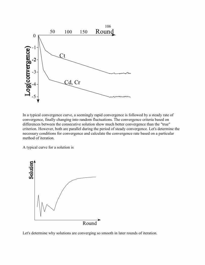
106

In a typical convergence curve, a seemingly rapid convergence is followed by a steady rate of

convergence, finally changing into random fluctuations. The convergence criteria based on

differences between the consecutive solution show much better convergence than the "true"

criterion. However, both are parallel during the period of steady convergence. Let's determine the

necessary conditions for convergence and calculate the convergence rate based on a particular

method of iteration.

A typical curve for a solution is

Let's determine why solutions are converging so smooth in later rounds of iteration.

Round0

-1

-2-2

-3

50 150100

-4

-5

Ct

Cd, Cr

Round

107

The stationary iteration can be presented in a form

x(n+1)= B x(n) + c

Decompose B into eigenvalues and eignevectors. For nonsymmetric B, these are complex

B = VE',

where E is diagonal, eii are eigenvalues, and rows of V: vi are eigenvectors, which are orthogonal

and normalized only for symmetric B

The successive stages of the iteration can be presented as:

x(1)= B x(0) + c

x(2)= B x(1) + c =B (B x(0) + c) +c = B2x(0) +Bc + c

x(3)= B x(2) + c =B (B2x(0) +Bc + c) +c = B3x(0) +B2c + Bc + c

...

x(n)=Bnx(0) +Bn-1c +..+ Bc + c

and, assuming that x(0) = 0

x(n) - x(n-1) = Bn-1c

Because the product Bn is

VEV- VEV- ... VEV- = VEn V-

therefore

𝐵𝑛𝑐 = 𝑉𝐸𝑛𝑉−𝑐 = ∑𝑒𝑖 𝑣𝑖𝑣𝑖′𝑐 = 𝑒𝑙

𝑛 ∑(𝑒𝑖

𝑒𝑙)𝑛

𝑣𝑖𝑣𝑖′𝑐

𝑖

𝑛

𝑖

Arrange VEV so that the absolute values of the eigenvalues are ordered in the descending order

|e1| ≥ |e2| ≥ ... ≥ |em|

If we assume |e1|>|e2| then for sufficiently large n

|𝑒𝑖

𝑒𝑙|𝑛

≈ 0 𝑓𝑜𝑟 𝑖 > 𝑗

and

Bnc ≈ e v1 v1'1'c = |e1|

n f

Then

x(n) = x(n-1) + Bn-1c = x(n-1) + |e1|n-1 f

108

The last expression shows for convergence |𝑒𝑙𝑛+1| < |𝑒𝑙

𝑛| ⇒ |𝑒𝑙| < 1, or that the largest

eigenvalue must be smaller than one.

It also shows that for large n the changes in the solutions will be predictable, where the same

vector f is added with a coefficient becoming e1 times smaller every next round. That predictable

change is the reason for a relatively flat convergence curve for larger n. We can rewrite the

formula for convergence criterion based on differences between the consecutive solutions

𝐶𝑑(𝑛)

=‖𝑥(𝑛) − 𝑥(𝑛−1)‖

‖𝑥(𝑛)‖≈

‖𝑒𝑙𝑛−1𝑓‖

‖𝑥(𝑛)‖∝ |𝑒𝑙|

𝑛−1

and

log(𝐶𝑑(𝑛)

) = 𝑛 log(|𝑒𝑙|) + 𝑐𝑜𝑛𝑠𝑡

Thus, the slope of the convergence curve for larger n is constant and determined by the largest

eigenvalue of the iteration matrix.

Since for large n the solutions increase predictably, one can approximate x(∞). From

x(n) = x(n-1) + Bnc = x(n-1) + |e1|n-1 f

the formula for x(∞) will be

We can estimate e1 and e f directly from the iteration

and

|e -1| f = x(n) - x(n-1)

so the formula for x(∞) becomes

This formula may not work when eigenvalues are too close or when x(n) - x(n-1) is very small and

therefore contains large rounding errors. However, it is usually accurate enough for determination

of the true convergence criterion

𝐶𝑡(𝑛)

=‖𝑥(𝑛) − 𝑥‖

‖𝑥‖≈ [1 −

𝐶𝑑(𝑛)

𝐶𝑑(𝑛−1)

]

−1

𝐶𝑑(𝑛)

Example

Let Cd(100) =1.105*10-3, Cd

(101) =1.008*10-3, indicating three significant digits. The real accuracy

is close to

Ct(101) ≈1/(1-1.008/1.105) Cd

(101) ≈ 11 Cd(101)

109

so it is 11 times lower than that indicated by Cd(101).

Conclusions

1. Initial convergence is fast because all eigenvalues contribute to the convergence,

2. In later rounds, the convergence is determined by the largest eigenvalue of the iteration matrix,

3. After many rounds, the convergence reaches the limit of accuracy of computer floating point

numbers.

4. Good convergence rate is determined by steep slope of the convergence criterion and not by its

absolute value,

5. The criterion based on differences in solutions between consecutive rounds of iteration can

grossly overstate the accuracy.

Properties of the Jacobi iteration

The Jacobi iteration leads to very simple programs because the expression

b-Ax is easy to obtain for any format of A. In general, Jacobi converges for matrices diagonally

dominant, where aii > aij, but usually the MME do not satisfy this condition. In practice, Jacobi

diverges with more than one fixed effect and with animal-additive or dominance effect.

To converge with many fixed effects, the following modifications are generally successful:

- impose constrains on fixed effects, for example by forcing the sum of solutions for each

fixed effect except the first one to 0; the constrain by setting unnecessary equations to zero results

in poor convergence, or

- update only one effect at a time

To converge with animal-additive or dominance effect, extend Jacobi to second-order Jacobi (also

called Chebyshev-accelerated)

x(n+1)= x(n) + α(x(n) -x(n-1)) + β D-1 (b - A x(n))

where α and β are iteration parameters, which are adjusted for the best convergence. In the animal

model, the good parameters are α=.7-.9 and β=1. In the dominance model, additionally β = .4-.6.

The Jacobi iteration is of interest only when the LHS is not available explicitly, as with iteration

on data.

110

Properties of the Gauss-Seidel and SOR iterations

The GS and SOR iterations converge for all symmetric semipositive-definite matrices. No

constrains are necessary for redundant equations or fixed effects. The disadvantage is that

elements of A must be available sequentially, row by row. As will be shown later, SOR has

advantage over GS only for effects with nondiagonal blocks.

Practical convergence issues

Predictions of breeding values for genetic evaluation need to be calculated with very limited

precision, no more than 2 decimal digits. Such precision is obtained with 5-15 rounds in a single-

trait sire model, 30-100 rounds in a single-trait animal model. With models with multiple traits

and the maternal effect, the number of rounds can increase to > 500. One way of increasing the

convergence rate for multiple traits is to set the MME within traits and decompose

A = L + D + L'

so that D would include diagonal blocks of traits, and possible blocks of direct and maternal

effects. Such a modification described by VanVleck and Dwyer (1985; JDS). Then, the

convergence rate with multiple traits is comparable to that with a single-trait.

Jacobi by effects, where only one effect is solved at a time, would be equivalent to a mixed

iteration where the outer iteration is GS and the inner iteration is Jacobi. Note that for fixed

effects where the diagonal blocks for effects are diagonal, Jacobi by effects is equivalent to

Gauss-Seidel. A disadvantage of block iteration is increased storage for diagonal elements.

MME are usually not of full rank. While regular Jacobi iteration requires "sum to zero" for all

fixed effects but one, Jacobi-by-effect, GS and SOR handle the MME well and do not need any

constrains.

Determination of best iteration parameters

Some iterations, including SOR and second order Jacobi, require the choice of quasi-optimal

iteration parameters. Those parameters can be selected in a few ways, by

1. setting the iteration matrix B for several parameters, calculating eigenvalues, and selecting

parameters corresponding to the smallest e1; hard to do for large systems of equations

2. running the iteration many times with different parameters and selecting the parameter with

the best convergence rate in later rounds of iteration (lowest e1),

3. updating the parameters during the course of iteration, as in Hageman et al. (1981?) or

ITPACK. Usually parameters quasi-optimal for one data set remain quasi-optimal for

similar data sets.

111

Strategies for iterative solutions

Solving by effects

Consider a model

𝑦 = ∑𝐹𝑖𝑧𝑖 + 𝑒

𝑖

where fi may be either random or fixed effect. The MME assuming for simplicity R=I are

[ 𝐹1

′𝐹1 + 𝐺1−1 𝐹1

′𝐹2 𝐹1′𝐹3 .

𝐹2′𝐹1 𝐹2

′𝐹2 + 𝐺2−1 𝐹2

′𝐹3 .

𝐹3′𝐹1 𝐹3

′𝐹2 𝐹3′𝐹3 + 𝐺3

−1 .. . . .]

[ 𝑓1𝑓2̂𝑓3̂. ]

= [

𝐹1′𝑦

𝐹2′𝑦

𝐹3′𝑦.

]

This system of equation is equivalent to block equations

[𝐹1′𝐹1 + 𝐺1

−1]𝑓1̂ = 𝐹1′(𝑦 − 𝐹2𝑓2 − 𝐹3𝑓3) = 𝐹1

′𝑦1(∗)

[𝐹2′𝐹2 + 𝐺2

−1]𝑓2̂ = 𝐹2′(𝑦 − 𝐹1𝑓1 − 𝐹3𝑓3) = 𝐹2

′𝑦2(∗)

[𝐹3′𝐹3 + 𝐺3

−1]𝑓3̂ = 𝐹3′(𝑦 − 𝐹1𝑓1 − 𝐹2𝑓2) = 𝐹3

′𝑦3(∗)

..........................................................................................

where yi(*) is vector of observations adjusted for all effects but i. Instead of solving the full MME

iteratively, it is possible to solve each block separately by any method, and repeat the solving by

blocks until convergence.

Creating the adjusted observations is simple. For example, if a model for one observation is

5.2 = c1 + a20 + p15 + e

and if

𝑐1̂ = 1.4, 𝑎20̂ = 5.2, 𝑝15̂ = 3.8

the value of y adjusted for all effects except a would be

5.2 - 1.4 - 3.8 = 0.0

Iteration on data (matrix-free iteration)

If MME cannot be stored in memory but can be created on disk, the system of equations can be

solved by repeatedly reading the MME from disk. However, reading from disk is relatively slow.

112

The size of the LHS of MME can be 10 times or larger than the size of data, with difference

increasing with the number of traits and effects. Therefore instead of reading the MME from disk

it may be faster (and simpler) to read the much smaller data from disk and recreate necessary

parts of MME each round.

Iteration on data (I.D.) is very simple when the iteration method involves A only in the expression

Ax(n)

This expression can be created as follows:

Original program I.D. program

...

A(i,j)=A(i,j)+z

...

call solve(A,b,x)

...

do round=1,p

AX=0; D=0

...

...

if (i == j) D(i)=D(i)+z

AX(i)=AX(i)+z*x(j)

...

...

! This is for Jacobi iteration only

do i=1,neq

x(i)=x(i)+(b(i)-AX(i))/D(i)

end do

end do

.....

The statements to set-up D and AX are added for parts of the program corresponding to

contributions due to records and to contributions due to relationships.

When the iteration updates only one effect in one round, the modifications would be

do round=1,p

AX=0; D=0

do e1=1,neff

...

...

if (i == j) D(i)=D(i)+z

AX(i)=AX(i)+z*x(j)

...

...

! This is for Jacobi iteration only

do i=sum(nlev(1:e1-1)+1,i=sum(nlev(1:e1)

x(i)=x(i)+(b(i)-AX(i))/d(i)

113

enddo

end do

end do

Please see that the program statements related to relationship contributions are not shown above

separately. For the iteration that needs only the matrix-vector product Ax, the data and pedigree

files need not be in any particular order. For multiple-trait block iteration, the programs would be

modified to create block-diagonal D.

The same strategy can be used in PCG except that the product to derive can be either Ax or Ap.

The implementation of the Gauss-Seidel or SOR iteration is more difficult because LHS needs to

be available one row at a time. To do so:

- for e effects, create e copies of the data file, each sorted for different effect

- for pedigree file, create 3 copies, sorted by animal, sire and dam, respectively.

- solve as follows:

do e=1,neff

rewind i

.....

.....

do l=1,nlev(i)

d=0

ax=0

current=address(e,l)

.....

.....

do

"read file sorted by level l until the end of level l"

.....

.....

if (i == current) then

if (i==j) d=d+z

ax=ax+z*x(j)

endif

end do !of reading the level l

!

if (e is animal effect) then

do

read pedigree line with animal l &

as either animal, sire or dam

....

....

if (i == current) then

if (i==j) d=d+z

114

ax=ax+z*x(j)

endif

enddo

endif

if (e is other random effect then)

"create other random effect contributions'

endif

! solve for level l of effect e

x(current)=x(current)+ (b(current)-ax)/d

.....

.....

enddo

......

......

enddo

Schaeffer and Kennedy (1996) have shown a technique where for e effects one needs only e-1

sorted files. Another technique that reduces the need for sorted files is to solve small effects by a

finite method. This technique is used in PEST. For effects where diagonal blocks for effect are

diagonal matrices, Jacobi_by_effect is equivalent to GS, and no sorting is required.

Indirect representation of mixed-model equations

The mixed model equations, especially those simpler ones, can be solved without the use (and

knowledge) of any matrices (Misztal and Gianola, 1987). The indirect iteration gives insight into

the workings of GS and J methods.

Assume a single-trait model

yijkl = hi + gj + sk +eijkl, σe2 /σs

2 = α

where yijkl is a yield of a cow in herd i, genetic group j and sire k. The contribution of one record

yijkl to LHS and RHS is

115

LHS RHS

hi . gj . sk

. . . . . . .

hi . 1 1 1 yijkl

. . . . . . .

gj . 1 1 1 yijkl

. . . . . . .

sk . 1 . 1 . 1 yijkl

. . . . . . .

All the contributions corresponding to the row of hi result in an equation

∑(ℎ𝑖 +

𝑗𝑘𝑙

𝑔𝑗 + 𝑠𝑘) = ∑𝑦𝑖𝑗𝑘𝑙

𝑗𝑘𝑙

The GS iteration for hi would be

ℎ𝑖 = ℎ𝑖 + (𝑅𝐻𝑆 − 𝐿𝐻𝑆 [ℎ𝑔𝑠])/𝑛ℎ𝑖

or

ℎ𝑖 = ℎ𝑖 +[∑ (𝑦𝑖𝑗𝑘𝑙 − ℎ𝑖 −𝑗𝑘𝑙 𝑔𝑗 − 𝑠𝑘)]

𝑛ℎ𝑖

= [∑ (𝑦𝑖𝑗𝑘𝑙 −𝑗𝑘𝑙 𝑔𝑗 − 𝑠𝑘)]

𝑛ℎ𝑖

= (𝑦𝑖𝑗𝑘𝑙 − 𝑔𝑗 − 𝑠𝑘)̅̅ ̅̅ ̅̅ ̅̅ ̅̅ ̅̅ ̅̅ ̅̅ ̅̅ ̅̅ ̅

The solution for hi is an average of observations that include hi adjusted for all the other effects.

Similarly, we can derive equations for gj and sk

𝑔𝑗 = (𝑦𝑖𝑗𝑘𝑙 − ℎ𝑖 − 𝑠𝑘)̅̅ ̅̅ ̅̅ ̅̅ ̅̅ ̅̅ ̅̅ ̅̅ ̅̅ ̅̅ ̅

𝑠𝑘 = (𝑦𝑖𝑗𝑘𝑙 − ℎ𝑖 − 𝑔𝑗)̅̅ ̅̅ ̅̅ ̅̅ ̅̅ ̅̅ ̅̅ ̅̅ ̅̅ ̅̅ ̅ 𝑛𝑠𝑘

𝑛𝑠𝑘+ 𝛼

The regression towards the mean in the last equation is due to sk being the random effect.

116

In the GS iteration, hi will be solved first, followed by gj and then by sk. In the Jacobi iteration, all

effects will be solved simultaneously.

Example

i j k yijkl

1 1 1 17

1 1 2 10

1 2 1 12

1 2 2 7

2 1 1 14

2 1 2 9

2 2 1 11

2 2 2 4

Assume that α=8 and that the initial solutions are 0. The first round solutions by GS are

h1 = (17+10+12+7)/4 = 11.5

h2 = (14+9+11+4)/4=9.5

g1 = [(17-11.5) + (10-11.5) + (14-9.5) + (9-9.5)]/4=2

g2 = [(17-11.5) + (7-11.5) + (11-9.5) + ((4-9.5)]/4=-2

s1 = 1/(4+8) [ (17-11.5-2) + (12-11.5 -(-2)) + (14-9.5-2) + (11-9.5-(-2))]=1

s2 = -1

The solutions will remain identical the next round so the convergence for this special balanced

case was reached in 1 round.

In Jacobi

h1 = (17+10+12+7)/4 = 11.5

h2 = (14+9+11+4)/4=9.5

g1 = (17 + 10+ 14 + 9)/4=12.5

g2 = (17+7+11+4)/4=8.5

s1 = 4/(4+8) (17+12+14+11)/4=4.5

s2 = 4/(2+8) (10+7+9+4)/4 = 2.5

During the next round the solutions will diverge. However, J will converge if the system of

equations is made full rank by setting the sum of all g solutions to 0. Id additionally the sum of s

solutions is set to 0, J will converge in one round.

117

That convergence in one round is a special property of GS and constrained J, and it is missing

from other methods. This is why J and GS and their modifications are naturally suited to MME.

Note that second-order Jacobi and SOR won't converge in one round in the example. One way to

make them do it is not to use any relaxation factors for fixed effects and for random effects with

the diagonal (co)variance matrix.

Animal model

In the model with groups, the contributions to the left hand side are:

LHS

ai . si (or gsi) . dj (or gdi)

. . . . . .

ai . 2αvi -αvi -αvi

. . . . . .

si (or gsi) . -αvi -αvi/2 -αvi/2

. . . . . .

dj (or gdi) . -αvi . -αvi/2 . -αvi/2

. . . . . .

ai, si and di are animal, and sire and dom solutions, respectively, g's are unknown parent groups if

sire or dam are missing, α is variance ratio and

vi = 2 /(4- number of known parents)

Calculate the quantity

z = - α vi( 2 ai - di - si )

The contribution to the adjusted right hand side (b-AX) from each pedigree line is:

to animal

- α vi( 2 ai - di - si ) = z

to sire (or sire unknown parent group)

α vi( 2 ai - di - si )/2 = -z/2

to dam (or dam unknown parent group)

α vi( 2 ai - di - si )/2 = -z/2

The corresponding changes to the diagonal would be:

to animal

2 α vi

to sire (or sire unknown parent group)

α vi /2

to dam (or dam unknown parent group)

α vi /2

Example

118

Consider the "dairy" repeatability model

yijkl = mi + pj + ak + eijkl

where yijkl is yield of cows in management groups mi, with additive value ak and permanent

environment pj, and

var(p)=Iσp2, var(a)=Aσa

2, σe2/σa

2=α, σe2/σp

2=β

The matrix-free equations are

𝑚𝑖 = (𝑦𝑖𝑗𝑘𝑙 − 𝑝𝑗 − 𝑎𝑘)̅̅ ̅̅ ̅̅ ̅̅ ̅̅ ̅̅ ̅̅ ̅̅ ̅̅ ̅̅ ̅

𝑝𝑗 = (𝑦𝑖𝑗𝑘𝑙 − 𝑚𝑖 − 𝑎𝑘)̅̅ ̅̅ ̅̅ ̅̅ ̅̅ ̅̅ ̅̅ ̅̅ ̅̅ ̅̅ ̅̅ 𝑛𝑝𝑗

𝑛𝑝𝑗+ 𝛽

𝑎𝑘

= ∑ (𝑦𝑖𝑗𝑘𝑙 − 𝑚𝑖 − 𝑝𝑗) − 𝛼𝑣𝑘(−𝑑𝑘 − 𝑠𝑘) − 𝛼 ∑ 𝑣𝑘𝑙(−𝑝𝑟𝑑𝑘𝑙 + 𝑚𝑎𝑡𝑒𝑘𝑙)

𝑝𝑟𝑜𝑔𝑒𝑛𝑖𝑒𝑠 𝑜𝑓 𝑘𝑙=1𝑟𝑒𝑐𝑜𝑟𝑑𝑠 𝑜𝑓 𝑘

𝑛𝑎𝑘+ 2𝛼𝑣𝑘 + 𝛼/2∑ 𝑣𝑘𝑙

𝑝𝑟𝑜𝑔𝑒𝑛𝑖𝑒𝑠 𝑜𝑓 𝑘𝑙=1

where prkl and matekl are the progeny and mate of the l-th mating of the k-th animal, respectively,

and vkl is the corresponding residual (=.5 if mate is known and 1/3 if mate is replaced by

unknown parent group).

The extension of these rules to multiple traits, maternal effects etc. can be done following the

above methodology. For GS iteration, it was done by Kennedy and Schaeffer (1986, WCGALP).

Summary of iteration strategies

The GS and SOR iterations are the methods of choice when the coefficient matrix can be stored in

memory and simplicity is important. This would usually require memory of 100-1000

bytes/equations. The iteration on data by modifications of Jacobi would be the next choice for

simpler models, with memory requirements of 12-16 bytes/equation. However, the method of

choice nowadays seems to be PCG. Despite a seemingly complicated code, PCG is very easy to

implement because the only compute-intensive operations are Ax or Ap, especially with Fortran

90 with vector instructions. PCG with diagonal preconditioner converged for all attempted

models, including multiple trait, random regressions, with maternal effect and dominance. The

convergence rate was as good or better as J or SOR. Also, there are no acceleration parameters to

determine. One disadvantage of PCG is that it requires more memory: 36-56 bytes/ equations, but

this is not as much of a problem as it used to be.

119

Variance components

Out of very many methods for estimating variance components, three types are in popular use

today (1998). They are:

1. REML

2. Bayesian methods via Gibbs-sampling, also called Markov Chain Monte Carlo (MCMC),

3. Method R.

REML is popular because of resistance to selection bias and the estimates are always within the

parameter space. Its disadvantages include high cost for large models and relatively difficult

programming especially for nonstandard models although various implementations of REML

differ widely in their computing properties.

Bayesian methods via Gibbs-sampling result in simple programs even for complicated models,

and have good theoretical properties. Their disadvantage include slow convergence because of

the Monte-Carlo origin and therefore very long running time for larger problems.

Method R is applicable to very large systems of equations and is simple to implement for

common models. However, the sampling error is higher than in the above methods, and incorrect

fixed effects can result in drastically biased estimates. Also, for multiple traits there are only

approximations.

REML

Let the model be

y = Xβ + e

where the distribution of y is multivariate normal with mean Xβ and variance V,

y ~ MVN(Xβ, V)

or

Var(e) = V and E(y) =Xβ

Following Quaas (1990), the likelihood of β and V is

𝐿(𝛽, 𝜑; 𝑦) =1

√2𝜋|𝑉|𝑒

−(𝑦−𝑋𝛽)′𝑉−1(𝑦−𝑋𝛽)2

where φ is a vector or a matrix of variance components in V. This can be simplified to

𝑙𝑛𝐿(𝛽, 𝜑; 𝑦) = −12⁄ [ln(2𝜋) + ln|𝑉| + (𝑦 − 𝑋𝛽)′𝑉−1(𝑦 − 𝑋𝛽)]

The maximum likelihood (ML) estimates can be obtained by maximizing ln L. The ML estimates

of variance components depend on fixed effects because the degrees of freedom due to estimating

120

the fixed effects are not taken into account. In restricted maximum likelihood, y is replaced by

My such that

MX= 0 ⇒ My = Me

which is equivalent to integrating the fixed effects from the ML likelihood. In subsequent

derivations M cancels out, and the log of the restricted maximum likelihood becomes

𝑙𝑛𝐿(𝜑; 𝑦) = −12⁄ {ln(2𝜋) + ln|𝑋′𝑉−1𝑋| + 𝑦[𝑉−1 − 𝑉−1𝑋(𝑋′𝑉−1𝑋)𝑋′𝑉−1]𝑦}

Most of the research in REML went into simplifying the above likelihood for particular models

and into maximizing that likelihood. For mixed models, the log likelihood is proportional to

−𝑙𝑛𝐿(𝜑; 𝑦) ∝ 𝑙𝑛|𝑅| + 𝑙𝑛|𝐺| + 𝑙𝑛|𝐶∗| + 𝑦′𝑅−1(𝑦 − 𝑋�̂� − 𝑍�̂�)

where C* is the coefficient matrix of the MME converted to full-rank; the determinant of a

singular matrix is 0.

For

𝑅 = [𝑅1 0 .0 𝑅2 .. . .

] , 𝐺 = [𝐺1 0 .0 𝐺2 .. . .

]

where Ri is the residual (co)variance matrix for observation i, and Gj is the (co)variance matrix for

random effect j, the components of the likelihood can be further simplified to

𝑙𝑛|𝑅| = ∑𝑙𝑛|𝑅𝑖|,

𝑖

𝑙𝑛|𝐺| = ∑𝑙𝑛|𝐺𝑖|

𝑖

In particular, for specific G's,

𝑙𝑛|𝐺𝑎0⨂𝐴| ∝ 𝑛𝑎𝑙𝑛|𝐺𝑎0|, ln|𝐺𝑖0⨂𝐼| ∝ 𝑛𝑖𝑙𝑛|𝐺𝑖0|

where na and ni are the number of levels.

The REML estimates are derived by maximization

�̂�:max 𝑙𝑛𝐿(𝜑; 𝑦)

φ

by one of the many maximization algorithms for nonlinear functions.

REML is relatively easy to evaluate. Matrices Ri and Gi0 are small. ln|C*| can be calculated from

the Cholesky decomposition of LHS. Also, solutions can be obtained by Cholesky decomposition.

121

The simplest maximization is derivative-free:

a) choose a derivative-free maximization subroutine from a library (IMSL, "Numerical

Recipes","www.netlib.org",..)

b) write a function L(variance components)

c) apply a) to b)

The computational constrain in derivative free methods would be time to calculate the

determinant.

The alternate way to maximize the REML would be by using the first derivative,

�̂�:δ 𝑙𝑛𝐿(𝜑; 𝑦)

𝛿𝜑= 0

which is a problem of finding zeroes of a multidimensional nonlinear function. In single traits,

this leads to the following equations

�̂�𝑖2 =

�̂�𝑖′𝐴𝑖

−1�̂�𝑖 + �̂�𝑒2𝑡𝑟(𝐴𝑖

−1𝐶𝑖𝑖)

𝑛𝑖

where ni is the number of levels of random effect i, σi2Ai is its (co)variance matrix, and Cii is a

diagonal block of the inverse of C corresponding to effect i. This formula can be derived

differently as EM REML. A faster converging version of the same formula is

�̂�𝑖2 =

�̂�𝑖′𝐴𝑖

−1�̂�𝑖

𝑛𝑖 − 𝑡𝑟(𝐴𝑖−1𝐶𝑖𝑖)

�̂�𝑒2

�̂�𝑖2

where ni is the number of levels in the i-th random effect. The residual is estimated as

�̂�𝑒2 =

𝑦′(𝑦 − 𝑋�̂� − ∑ 𝑍𝑖𝑖 �̂�𝑖)

𝑛𝑟 − 𝑟(𝑋′𝑋)

where nr is the number of records and r(X'X) is the rank of the fixed-effect part of the MME. In

the first-derivative REML, the largest expense is in calculating the inverse of C. The trace can be

computed as

𝑡𝑟(𝐴𝑖−1𝐶𝑖𝑖) = 𝑠𝑢𝑚(𝐴𝑖

−1#𝐶𝑖𝑖)

or as the sum of Ai-1 and Cii multiplied directly, element by element. When Ai

-1 is sparse, one

does not require all elements of Cii but only those that are nonzero in Cii, or a small fraction of all

inverse elements of C. The sparse inverse described before contains all the inverse elements

nonzero in Ai-1. Computing that inverse from sparse factorization costs twice more than

122

computing the factorization alone, and almost no extra memory. Thus, the most compute-

intensive operation in one step of first-derivative REML is three times more expensive than a

similar operation in derivative-free REML.

For multiple traits, denote G as

𝐺 = [

. . .

. 𝜎𝑖𝑗𝑘𝑙2 𝐴𝑖𝑗𝑘𝑙 .

. . .]

and let the system of equations be

(𝑊′𝑅−1𝑊 + 𝐺−1)𝜃 = 𝑊′𝑅−1𝑦, 𝑊 = [𝑋, 𝑍], 𝜃 = [�̂�

�̂�]

where Aijkl can either be a numerator relationship matrix or an identity matrix for a block

corresponding to effects i and j and traits k and l. Denote

Aijkl = Aijkl-1

In multiple traits and the first-derivative REML, computations are similar to single-traits for

random effect variances

�̂�𝑖𝑗𝑘𝑙2 =

�̂�𝑖𝑘′ 𝐴𝑖𝑗𝑘𝑙�̂�𝑗𝑙 + 𝑡𝑟(𝐴𝑖𝑗𝑘𝑙𝐶𝑖𝑗𝑘𝑙)

𝑛𝑖𝑘

where δij =1 if i=j and 0 otherwise, and nik is the number of levels for effect i and trait k (nik = njl).

The formula for the residual variances when all traits are recorded is

𝜎𝑒𝑖𝑗2 =

�̂�𝑖′�̂�𝑗+𝑡𝑟(𝐶𝑖𝑗𝑊𝑖

′𝑊𝑗)

𝑛𝑟, 𝑤ℎ𝑒𝑟𝑒 �̂�𝑖 = 𝑦𝑖 − 𝑋𝑖�̂�𝑖 − 𝑍𝑖�̂�𝑖

where nr is the number of records. With missing traits, the formulas are more complicated to write

(but not to compute) and can be found for example in Mantysaari and VanVleck (1989).

Let

𝑅𝑘− = (𝑃𝑘𝑅0𝑃𝑘)

−

be a matrix of residual variances for observation k, where Pk is a diagonal matrix with 1 in

diagonals corresponding to present traits and 0 otherwise. Define Eij as matrix with 1 in position

(i,j) and (j,i) and 0 elsewhere. Then compute the following:

𝑄𝑘,𝑖𝑗 = 𝑅𝑘−𝐸𝑖𝑗𝑅𝑘

−, 𝑖 = 1,… , 𝑡, 𝑗 = 𝑖, … , 𝑡

𝑄𝑖𝑗 = ∑𝑄𝑘,𝑖𝑗, 𝐸𝑄𝐸𝑖𝑗 =

𝑛

𝑘

∑�̂�𝑘′

𝑘

𝑖

𝑄𝑘,𝑖𝑗�̂�𝑘, 𝑇𝑅𝑄𝑊𝐶𝑊𝑖𝑗 = ∑𝑡𝑟(𝑄𝑘,𝑖𝑗𝑊𝑘𝐶𝑊𝑘′)

𝑘

𝑖

123

Using the notation:

𝑄𝑖𝑗 = {𝑞𝑖𝑗,𝑙𝑚}

next round estimates are obtained by solving the system of equations:

[ 𝑞11,11 2𝑞11,12 … 2𝑞11,1𝑡 𝑞11,22 … 𝑞11,𝑡𝑡

𝑞12,11 2𝑞12,12 … 2𝑞12,1𝑡 𝑞12,22 … 𝑞12,𝑡𝑡

…𝑞1𝑡,11 2𝑞1𝑡,12 … 2𝑞1𝑡,1𝑡 𝑞1𝑡,22 … 𝑞1𝑡,𝑡𝑡

𝑞22,11 2𝑞22,12 … 2𝑞22,1𝑡 𝑞22,22 … 𝑞22,𝑡𝑡

…𝑞𝑡𝑡,11 2𝑞𝑡𝑡,𝑡1 … 2𝑞𝑡𝑡,1𝑡 𝑞𝑡𝑡,22 … 𝑞𝑡𝑡,𝑡𝑡 ]

[ �̂�𝑒11

2

�̂�𝑒122

…�̂�𝑒1𝑡

2

�̂�𝑒222

…�̂�𝑒𝑡𝑡

2 ]

=

[ 𝑒𝑞𝑒11 + 𝑡𝑟𝑞𝑤𝑒𝑤11

𝑒𝑞𝑒12 + 𝑡𝑟𝑞𝑤𝑒𝑤12

…𝑒𝑞𝑒1𝑡 + 𝑡𝑟𝑞𝑤𝑒𝑤1𝑡

𝑒𝑞𝑒22 + 𝑡𝑟𝑞𝑤𝑒𝑤22

…𝑒𝑞𝑒𝑡𝑡 + 𝑡𝑟𝑞𝑤𝑒𝑤𝑡𝑡 ]

Caution: blocks of inverse Cij and Cijkl for covariance are not necessarily symmetric. This may

create computing problems if sparse matrix software operates on symmetric matrices only.

Second derivatives of REML or their expectation cannot be easily computed using sparse matrix

computations because they require computations of off-diagonal blocks of C. Jensen et al. (1996-

7) have shown that the average of second derivatives and their expectations results in cancellation

of terms that are hard to compute. Their method based on the ideas of R. Thompson was called

"Average Information" REML. In this method, the most important computation is of matrix F

defined by n x p, where n is the number of observations and p is the number of different variance

components including the residuals. Matrix F is composed of weighted solutions or residuals.

Then the matrix of Average Information, which is used later as the approximation of the matrix of

second derivatives, is:

𝐼𝑎 = 𝐹′𝑅−1𝐹 − 𝑇′𝑊𝑅−1𝐹, 𝑇 = 𝐶−1𝑊′𝑅−1𝐹

where T is solution to the mixed model equations with cluster of T substituting for y. Although

this algorithm is fast when it converges, it requires heuristics when Ia is not positive definite and

its implementation is quite complex.

124

General Properties of Maximization Algorithms

The problem is to find

x: max f(x)

x

where f(x) is a nonlinear function. The algorithms for the maximization can be categorized by

their use of derivatives of f(x):

Derivative-free - Only function values available, no derivatives available.

First-derivative - df(x)/dx available

Second-derivative - d2f(x)/dx2 and df(x)/dx available

The underlying mechanisms of these three methods are presented below for a one-dimensional

case. It is assume that the function to be maximized has exactly one maximum.

The example below shows two points that could be made available in a derivative free method.

Each point provides the value of the function but does not indicate the direction of the maximum.

Two points can show the direction of the increase, and three point can bracket the maximum.

In the first-derivative method, each derivative shows the direction of the maximum. Two

evaluation of the derivatives may bracket the maximum.

f(x)

125

In a second-derivative method, each point contains the quadratic approximation of the function

from that point. Thus one point is sufficient to obtain the first approximation of the maximum.

Unless the function is quadratic, in which case the second-derivative methods converge in one

step, all methods need to be applied iteratively.

In general, the more derivatives are available, the faster the method. However, if the function is

far from quadratic and a second-derivatives are used, next-round estimates may be far from

optimum or even out of bounds.

f(x)

x

f(x)

x

126

Derivatives may be hard to calculate. In that case, the higher derivative methods can be derived

by numerical differentiation

𝛿𝑓(𝑥)

𝛿𝑥𝑖=

𝑓(𝑥+∆𝑝𝑖)−𝑓(𝑥)

∆

and

𝛿𝑓2(𝑥)

𝛿𝑥𝑖𝛿𝑥𝑗=

𝛿𝑓(𝑥+∆𝑝𝑗)

𝛿𝑥𝑖−

𝛿𝑓(𝑥)

𝛿𝑥𝑖

∆

where pi is the i-th column of the identity matrix. Unfortunately, the derivatives thus obtained

have a lower accuracy than those obtained analytically. According to Press et al. (1986), the

number of significant digits in the derivatives calculated numerically cannot be higher than half

the number of significant digits in the original function. In general the selection of Δ is not an

easy one.

Some popular maximization algorithms

Downhill simplex (derivative-free)

One of the most popular derivative-free maximization algorithms is downhill simplex. It is

described in the animal breeding context by Boldman et al (1995) in the MTDFREML manual.

Let n be the number of parameters to find. Initially create n+1 vectors

x0, x1,.., xn

and calculate the functions f(xi)=fi ordered so that

f0>f1>...>fn

Choices on the maximization for one dimension are shown below.

best pointworstpoint

best point

middlepoint

Possible choices

127

The general algorithm is

do until convergence

Calculate the mean point:

xm= ave(x1,.., xm)

Calculate a reflection of the worst point against the center point:

xr = xm+α(tm-tp)

case

The new point is best!

fr > f0

Try even a better point

xb = xm+γ(xr-xm)

xn = better(xr, xb)

The new point is neither worst nor best f0 > fr > fp

Replace the worst point

xp == xr

The new point is almost worst

fp-1 >fr >fp

Contract to the opposite side of the worst point

xp = xm+β(xr-xm)

The new point is worst or equal

fr ≤ fp

Try contracting first to the worst point

xr = xm+β(xp-xm)

New point better

fr > fp

xp = xr

New point worse

fr <= fp

Contract in every direction towards the best point

xi=(xi+x0)/2 for i=1,.., n

end case

end do

Sample constants: α=1; β=.5; γ=2

Powell (derivative-free)

128

Set the initial point xbase

do until convergence

Find the "best" direction d by probing n dimensions

Find α such that:

max F(xbase +dα)

α

xnew = xbase + dα

enddo

Fixed point (first derivative)

Rearrange the equation

df(x)/dx = 0

to

x = g(x)

and solve as

x(n+1) = g(x(n))

The choice of g is critical to convergence. For example, the rearrangement of

√𝑥 −𝑥

√𝑥= 0 → (√𝑥)

(𝑛+1)=

𝑥

√𝑥(𝑛)

results in divergence, but a similar expression converges rapidly

2√𝑥 − √𝑥 −𝑥

√𝑥= 0 ⟹ (√𝑥)

(𝑛+1)=

√𝑥(𝑛)

+𝑥

√𝑥2

Newton (second derivative)

x(n+1) = x(n) - [d2f(x)/(dx)2]-1 df(x)/dx

Quasi-Newton (first derivative)

When second derivatives are difficult to compute, they may be approximated from first

derivatives. A method that approximates the second derivatives by finite differences is called

secant. For more information, see More and Wright (1993) or Woodford (1992)

Acceleration to EM (fixed point) estimates

The convergence rate in the EM algorithm can be slow, especially when the number of equations

relative to records is high. Denote the EM algorithm as

129

In the single trait, the iteration would be similar to

And the convergence curve would be similar to

Thus in later rounds, the convergence would be predictable, similar to convergence of stationary

methods in the linear system of equations. Little (1987) has shown that the convergence rate in

the EM algorithm is inversely proportional to the fraction of missing data. That fraction like the

largest eigenvalue of the iteration matrix is hard to compute analytically but can be approximated

during the progress of iteration.

For a single component, Schaeffer (1979) showed how results from two separate cycles of the EM

iteration can be used to extrapolate almost to the converged solutions. Misztal and Schaeffer

(1986) have shown that the em(x) approximately follows the geometric progression, and that the

y=x

y=em(x)

y=x

s(0)

s(0) s(1) s(2)

y

x

n

em(x(n))

130

final value can be extrapolated from estimates of successive rounds of EM iteration. Laird et al.

(1987) presented similar ideas for multiple dimensions.

Function em(x) is locally linear near the convergence point. Therefore, for large n, we can write

𝑠(𝑛+1) ≈ 𝑠(𝑛) + 𝛼[𝑠(𝑛) − 𝑠(𝑛−1)] Then

𝑠(𝑛+2) ≈ 𝑠(𝑛) + (𝛼 + 𝛼2)[𝑠(𝑛) − 𝑠(𝑛−1)] and finally

𝑠(𝑛+∞) ≈ 𝑠(𝑛) + (𝛼 + 𝛼2 + 𝛼3 + ⋯)[𝑠(𝑛) − 𝑠(𝑛−1)] = 𝑠(𝑛) +𝛼[𝑠(𝑛) − 𝑠(𝑛−1)]

1 − 𝛼

The extrapolation is beneficial only when the expression

𝛼𝑛𝑠(𝑛+1) − 𝑠(𝑛)

𝑠(𝑛) − 𝑠(𝑛−1)

becomes stable. Otherwise the extrapolation can deteriorate the convergence. Various types of

accelerations of the EM algorithm have been used successfully in packages DMUEM, and

REMLF90, with the reduction in the number of rounds by 2-10 times. Quasi-Newton

implementation in VCE, where only the first derivatives of the restricted likelihood are computed,

can be regarded as either approximated second-derivative algorithm, or accelerated EM.

131

Convergence properties of maximization algorithms in REML

Examine the cost of derivative and derivative-free algorithms in REML following Misztal (1995).

Convergence rate can be described in terms of accuracy as a function of the number of rounds of

iteration (Minoux 1986). Linear convergence means linear relationship between accuracy and

round of iteration, i.e., constant number of rounds is required for a gain of one extra digit of

accuracy. The fixed point iteration (EM algorithm) seems to have a linear convergence. In a

superlinear convergence, each round of iteration results in increasingly larger gains in accuracy.

Finally, in a n-step convergence, n steps are required to implement one round of iteration.

The convergence rate of maximization algorithms for general functions cannot be derived easily.

However, it could be derived for quadratic functions, and any twice-differentiable function,

including L, is locally quadratic. Then, the convergence of better derivative-free (DF) algorithms

such as Powell or Rosenbrock is n-step superlinear (Minoux 1986), and is dependent on n, the

dimension of the function being maximized. For better derivative (D) algorithms, such as quasi-

Newton (first-derivative) or Newton-Raphson (second-derivative), the convergence is superlinear

and does not depend on n (Bazaraa 1993; Minoux 1986). This leads to conjecture that better DF

algorithms converge, in general, n times slower than better D algorithms. N can be expressed in

terms of number of random effects, nr, and number of traits, nt, as:

n = (nr +1)nt(nt+1)/2 (4)

where the extra 1 is for the residual.

This difference in convergence rate is only approximate because differences exist within better D

or DF algorithms, and L is not quadratic. Also, more sophisticated methods may fail when the

starting point is far away from the maximum.

Cost of one step of D and DF in multiple traits

Let C be a coefficient matrix of the mixed model equations Assume that in DF, all computing

resources are spent in computing |C|. Also assume that in D, all computing resources are spent in

finding elements of C-1 corresponding to nonzero elements in C, or a sparse inverse of C. In

dense matrices, computing the inverse requires 3 times more arithmetic operations than

computing the determinant alone (Duff et al. 1989). Both operations require an equal amount of

storage. Approximately the same applies to the number of arithmetic operations in sparse matrices

(Misztal and Perez-Enciso 1993). The amount of storage required is 3 times larger for sparse

inversion if the inverse elements are computed by columns. Both options are supported under

FSPAK.

In multiple traits, assuming that almost all traits are recorded, the coefficient matrix of the

mixed model equations has nt times more equations and an average equation has nt times more

nonzero elements than in single traits. In dense matrices, the memory and computing

requirements for inversion or computing the determinant for a matrix nt larger increase as nt2 and

nt3, respectively. The same applies to sparse matrices, where memory and computing

requirements increase approximately as pq and pq2, where p is the number of equations and q is

the average number of nonzeroes per equation (Duff et al. 1989).

132

Cost of one unit of convergence relative to single trait estimation

Let C1d be the cost of one step of D in a single trait estimation. Let us compute costs of the same

level of convergence in nt traits for the DF and D algorithms: Cndf and Cn

d. If the DF convergence

is n times slower, computations for the matrix operations increase as nt3, and computing the

determinant costs a third of computing the inverse, the following formulas can be derived:

Cnd = nt

3 C1d (1)

Cndf = ⅓ (nr +1)nt(nt+1)/2 nt

3 C1d

= (nr +1) nt4(nt+1 )C1

d / 6 (2)

and the relative costs are:

Cnd /C

1d = nt

3 (3)

Cndf / C

1d = (nr +1) nt

4(nt+1 )/6 (4)

≈ (nr +1) nt5/6 (5)

Cndf /C

nd = (nr +1) nt(nt+1 )/6 (6)

≈ (nr +1) nt2/6 (7)

According to equation (3), the number of numerical operations in D increase cubically with the

number of traits. In equation (4), the cost of DF increases with the fifth power of the number of

traits. From equation (1) one can find that the costs of DF and D in models with 2 random effects

are similar in single trait. DF is less expensive with 1 random effect, and D is less expensive with

more than 2 random effects. In multiple traits, DF is nt2 more expensive than D.

Relative costs of multitrait DF REML evaluation using DF and D algorithms, computed

with formulae (3) and (4) are presented below

Number of traits Number of arithmetic operations Memory

requirements DF D

1 1 1 1

2 24 8 4

3 162 27 9

4 640 64 16

5 1875 125 25

6 4536 216 36

The table below shows time to calculate multiple trait REML estimates assuming that D and DF

both took a minute in single traits.

Number of traits Approximate CPU Time

133

DF D

1 1 min 1 min

2 ½ hr 8 min

3 2½ hrs ½ hr

4 11 hrs 1 hr

5 > 1 day 2 hrs

6 3 days 3½ hrs

Accuracy of the D and DF algorithms

In DF, if L(Θ) is computed with r significant digits, then Θ can be bracketed with at most r/2

significant digits (Press et al. 1989). Such a limit does not exist in D. Worse numerical accuracy

of the DF maximization is illustrated with in the Figure below, which shows a quadratic function

and its derivative.

The function is very flat, and the maximum of the function cannot be determined accurately by

looking at the function alone. The maximum can be determined much more precisely by finding

a zero of the function's first derivative.

Loss of accuracy in DF does not appear a problem at first. Most computations are done with

double precision, which corresponds to 15-17 significant decimal digits, and estimates with 1% or

134

2 significant digits of accuracy are considered sufficiently accurate in practice. However, the

likelihood function can have low accuracy for a variety of reasons. Some accuracy is lost due to a

roundoff error when summing all components of L. Components of that function may have

reduced accuracy. This particularly applies to the determinant, where the loss of accuracy could

result from lack of pivoting in Cholesky decomposition-based packages, poor conditioning of the

coefficient matrix and rounding errors associated with computing in large matrices. In multiple

traits, the coefficient matrix of the mixed model equations is composed of R0-1and Gi0

-1 -

covariance matrices between traits for residual and random effect i, respectively. Poor

conditioning of these matrices results in poor conditioning of W and subsequently low accuracy

of determinants and traces. R0-1and Gi0

-1 would be poorly conditioned numerically when traits are

highly correlated or linearly dependent. The loss of accuracy due to poor conditioning of C is

also present in derivative maximization, but it has smaller effect on the estimates because of better

numerical properties of the derivative maximization.

Another source of inaccuracy could arise in algorithms where derivatives are obtained

numerically by differentiation. For example, the Quasi-Newton algorithm can be so implemented

in DF, and one can regard other DF algorithms as using the numerical differentiation implicitly.

The accuracy of such differentiation is dependent on the step side and could be very low for steps

too large or too small. Subsequently, the accuracy would be dependent on parameters that define

the step size, and in particular could be good for some problems but poor for others.

135

Method R

The Method R was proposed by Reverter et al. (1994) and can be summarized as follows.

Let ui ~ N(0, Giσ),

Let i be a BLUP of ui based on all the data available, and let be a BLUP of ui based on a partial

data. Then

𝐶𝑜𝑣 (𝑢�̂�𝑝′

, 𝑢�̂�) = 𝑉𝑎𝑟(𝑢�̂�𝑝)

Define ri as the regression of predictions based on full data from those based on a partial data:

𝑟𝑖 =𝑢�̂�

𝑝′

𝐺𝑖−1𝑢�̂�

𝑢�̂�𝑝′

𝐺𝑖−1𝑢�̂�

𝑝

Define r = { ri } and s = {𝜎𝑒2 / 𝜎𝑖

2 }, where 𝜎𝑒2 is residual variance and s is vector of variance ratios.

Reverter et al. showed that for true variances,

E[r(s)] = 1.

For arbitrary x and one component

ri (x) > 1 ⇒ too small variance

ri(x) < 1 ⇒ too large variance.

For several components, the relationships between s and r are more complex. The problem of

finding such

�̂�: 𝑟(�̂�) = 1,

or

𝑟(�̂�) − 1 = 0

becomes a problem of solving a system of a nonlinear equations. It can be solved by a fixed point

iteration, Newton or quasi-Newton methods.

Method R can be generalized to multiple traits. Let 𝑢𝑖�̂� be a BLUP of uij based on all the data

available, and let 𝑢𝑖�̂�𝑝

be a BLUP of uij based on a partial data, where i spans the random effects

and j spans different traits.

Define rijkl as the regression of predictions based on full data from those based on a partial data for

effects i an dj and traits k and l, using terminology similar as in formula for multivariate REML

𝑟𝑖𝑗𝑘𝑙 =𝑢𝑖�̂�

𝑝′

𝐴𝑖𝑗𝑘𝑙

𝑢𝑗�̂�

𝑢𝑖�̂�𝑝′

𝐴𝑖𝑗𝑘𝑙

𝑢𝑖𝑗�̂�𝑝

For arbitrary x and one component

rijkl (x) > 1 ⇒ 𝜎𝑖𝑗𝑘𝑙2

too small

136

rijkl(x) < 1 ⇒ 𝜎𝑖𝑗𝑘𝑙2 too large.

No exact formulas are available for the residual variance but quasi-REML approximations were

used by Reverter et al. (1994) as follows

�̂�𝑒𝑖𝑖

2 =𝑒�̂�′𝑦𝑖

𝑛𝑟𝑖 − 𝑟𝑎𝑛𝑘(𝑋𝑖), 𝑤ℎ𝑒𝑟𝑒 𝑒�̂� = 𝑦𝑖 − 𝑋𝑖𝛽�̂� − 𝑍𝑖𝑢�̂�

where nri is the number of records in trait i, and

�̂�𝑒𝑖𝑗

2 =𝑒�̂�′𝑦𝑗 + 𝑒�̂�′𝑦𝑖

𝑛𝑟𝑖𝑗 − 𝑟𝑎𝑛𝑘(𝑋𝑖|𝑋𝑗)

where nrij is the number of records with both traits i and j recorded.

Method R is potentially less expensive than other methods because it only requires solutions to the

mixed model equations. Aside from being feasible computationally, Method R has several other

desirable properties. First, at least in single traits it returns estimates within the parameter space.

Second, it is resistant to bias caused by assortative mating because it considers the relationship

matrices. Also, it has been shown to be as resistant as REML to selection caused by non-random

replacements (Snelling, 1994) and incomplete reporting (Kaiser et al., 1996); Cantet and

Birchmeier (1998) initially reported bias under selection but later discovered that it was due to an

error in programming. Disadvantages of Method R would include a larger sampling variance than

other methods for the same data set, however, this disadvantage can be compensated by the ability

of Method R to consider much larger data sets.

Recently, Druet et al.(2001) has found that rijkl for covariances has a discontinuity because both its

nominator and the denominator can have a value of 0. They suggested alternative formulas. Exact

formulas for Method R in multiple traits are unknown.

Selection of partial data

The regressions do not specify which subset of data is selected. If subset is either a very small or a

very large percentage of the complete data set, up's will either be close to 0 or to u's, and the

regressions will have very large sampling error. Thus a size of 50% seems to be the a good choice.

Also by inappropriate selection of records, one can create bias for the model with the reduced data

set. A few types of subsets can be considered:

a) random,

b) by truncation over time

c) by truncation over later records with repeated records.

Random selection seems to be attractive, especially that subsets can be easily changed by changing

seed in a random number generator, and sampling variance can be approximated as variance of the

samples.

Method R can have poor properties when the model does not contain all fixed effects. For example,

in the study by Misztal et al. (1997), heritability for stature with single record per animal was 44%.

137

When multiple records were considered, the heritability has increased to almost 70%. After adding

the adjustment for age, the heritability dropped to 45%.

In simple models (Duangajinda et al., 2001), Method R has been shown to be mostly unbiased.

Biases were present with small data sets and with phenotypic selection across but not within

contemporary groups.

Numerical considerations

When the problem is small enough so that LHS can be factorized, REML would provide better

estimates than Method R. Therefore the value of Method R is in larger problems where solutions

can be obtained only by iteration. For calculation of breeding values, the accuracy of solutions is

usually not critical, and an accuracy of 2 decimal digits is more than satisfactory. For method R,

convergence to

r=1±0.0001

was found to be corresponding to the accuracy of the estimates of

s±5%

Thus, r=1±0.0001 or calculated with at least 4 decimal significant digits should be considered the

minimum. To get that accuracy, the solutions to MME should be calculated with even higher

accuracy, 5 to 6 significant digits. Otherwise convergence of Method R may not be achieved.

Because Method R results in a problem of solving the nonlinear system of equations, the

convergence of this method is more similar to D than to DF.

Solution of the nonlinear system of equations by Secant

The problem of finding

s : r(s) = 1

was solved by the secant method, which initially is equivalent to the Newton method, where

derivatives are computed by numerical differentiation. This algorithm is equivalent to assuming that

r = As +b

Consequently, approximate solutions are obtained setting r =1

1 = 𝐴�̂� + 𝑏 ⇒ �̂� = 𝐴−1(1 − 𝑏) A and b can be found when n+1 pairs of {s(i),r(s(i))} are available. Then,

r(s(i+1)) - r(s(i) )= A [s(i+1) - s(i)]

denoting

Δs = [s(1 )- s(0), s(2 )- s(1), ..,s(n )- s(n-1)]

Δr = [r(s(1)) - r(s(0)), r(s(2)) - r(s(1)), ..,r(s(n)) - r(s(n-1))]

the equation can be written as

Δr = A Δs

138

Thus

A = Δr (Δs)-1

b can be computed from the last point

b = r(s(n)) - A s(n )

which will result in

𝑠(𝑛+1) = 𝐴−1[1 − 𝑟(𝑠(𝑛)) + 𝐴𝑠(𝑛)] = 𝑠(𝑛) + Δ𝑠(Δ𝑟)−1[1 − 𝑟(𝑠(𝑛))]

The algorithm contains heuristics to ensure the convergence of the algorithm that would otherwise

result in estimates out of the parameter space or in a slower convergence rate.

1. Choose an initial guess s(0);

2. Assign n extra points as follows:

s(1) = s(0) + [δ1, 0, ..., 0]'

s(2) = s(1) + [0, δ2, 0, .., 0]'

......

s(n) = s(n-1) + [0, 0, .., δn]'.

3. Compute

{r(s(i))}, i = 0, n;

4. Compute differences:

Δs = [s(1 )- s(0), s(2 )- s(1), ..,s(n )- s(n-1)]

Δr = [r(s(1)) - r(s(0)), r(s(2)) - r(s(1)), ..,r(s(n)) - r(s(n-1))].

5. Compute next-round solutions

s(n+1) = s(n) + Δs (Δr)-1 [1 - r(s(n))]

5. Limit changes if too large:

maxchange = max( |si(n+1) - si

(n)| / |si(n)|)

I

if maxchange >γ then s(n+1) = s(n) +γ/maxchange (s(n+1) - s(n)).

6. If change large, compute n new points as before; if changes small, use all but one last point.

if max{|ri(s(n+1)) - 1|} > ε then

i

if max|si(n+1) - si

(n)| / |si(n)| > λ

I

set s(0) = s(n+1)

goto 2

else

s(0) = s(1), s(1) = s(2), ..,s(n-1) = s(n), s(n) = s(n+1)

goto 3.

7. Optionally, refine s using previously computed matrices

s(n+1) = s(n+1) + Δs (Δr)-1 [1 - r(s(n+1))].

139

In program JAADOM, changes between samples δi were chosen to correspond to a change of

variance of σe2/200, maximum relative changes were limited to γ = 0.7, the stopping criterion was ε

= 0.0001, and changes were regarded as small for λ = 0.1.

Numerical example

s(0) = [ 0.6, 0.9]'

s(1) = s(0) + {-0.0017946 ,0,...,0} = [0.5982054, 0.9]'

s(2) = s(1) + {0,-0.00403189 ,0,..,0} = [ 0.5982054, 0.89596811]'

r(s(0)) = [1.008687, 1.009935]

r(s(1)) = [1.008587, 1.009897]

r(s(2)) = [1.008552, 1.009800]

Δ𝑠 = [−0.0017946 0.0000

0.0000 −0.00403189]

Δ𝑟 = [−0.000100 −0.000035−0.000035 −0.000097

]

s(n+1) = [0.4940763 0.5808855]'

r(s(n+1) ) = [1.000021 0.9973247]'.

Because

1 - 0.9973247 = 0.0026753 > 0.0002,

s(0) is set to s(n+1), and computations are repeated from step 2. After that, the procedure converges at

s(n+1) = [0.4791, 0.6592]'

where

r(s(n+1)) = [1.00008, 0.99981]

It would be worthwhile to find out whether better performance could be obtained by quasi-Newton

methods.

140

Bayesian methods and Gibbs sampling

Following Wang et al. (1993), in the single-trait model

𝑦 = 𝑋𝛽 + ∑𝑍𝑖𝑢𝑖 + 𝑒

𝑖

the conditional distribution which generates the data is

𝑦ǀ𝛽, 𝑢1 … , 𝑢𝑒 , 𝜎𝑒2~𝑁(𝑋𝛽 + ∑ 𝑍𝑖𝑢𝑖 , 𝑅

𝑐𝑖 𝜎𝑒

2)

with the density

𝑝(𝑦ǀ𝛽, 𝑢1 … , 𝑢𝑐, 𝜎𝑢𝑐2 , 𝜎𝑒

2) ∝1

(𝜎𝑒2)𝑛/2 𝑒𝑥𝑝 {−

1

2𝜎𝑒2 (𝑦 − 𝑋𝛽 − ∑ 𝑍𝑖𝑢𝑖)′(𝑦 − 𝑋𝛽 − ∑ 𝑍𝑖𝑢𝑖)

𝑐𝑖

𝑐𝑖 }

One can specify distributions for β, u's and σ's. The distribution of β is flat

p(β) ∝ constant

The distribution for u's is multivariate normal

𝑢𝑖 ǀ𝐺𝑖, 𝜎𝑢𝑖2 ~𝑁(0,+𝐺𝑖 , 𝜎𝑢𝑖

2 )

with the density

𝑝(𝑢𝑖 ǀ𝐺𝑖 , 𝜎𝑢𝑖2 ) ∝ [

1

(𝜎𝑢𝑖2 )𝑛𝑢𝑖/2

𝑒𝑥𝑝 {−1

2𝜎𝑢𝑖2 (𝑢𝑖

′𝐺𝑖−1𝑢𝑖)}]

and for the variance components, it can be scaled inverted χ2

𝑝(𝜎𝑒2)−

𝑉𝑒2

−1𝑒𝑥𝑝(−

12𝑉𝑒𝑆𝑒

2

𝜎𝑒2

)

𝑝(𝜎𝑢𝑖2 )−

𝑉𝑢𝑖2

−1𝑒𝑥𝑝(−

12𝑉𝑢𝑖𝑆𝑢𝑖

2

𝜎𝑢𝑖2 )

where s..2 is the prior value and ν.. can be viewed as the degree of belief (uniformative prior for

ν..=0). The joint posterior density with flat priors is

𝑝(𝛽, 𝑢1, … , 𝑢𝑐,𝜎𝑢12 , … , 𝜎𝑢𝑐

2 , 𝜎𝑒2 ǀ𝑦) ∝ 𝑝(𝑦 ǀ 𝛽, 𝑢𝑖 , … , 𝑢𝑐,𝜎𝑢1

2 , … , 𝜎𝑢𝑐2 , 𝜎𝑒

2) 𝑝(𝛽)∑ 𝑝(𝑐𝑖=1 𝑢𝑖,𝜎𝑢𝑖

2 ) 𝑝(𝜎𝑒2)

or

141

𝑝(𝛽, 𝑢1, … , 𝑢𝑐,𝜎𝑢12 , … , 𝜎𝑢𝑐

2 , 𝜎𝑒2 ǀ𝑦) ∝

1

(𝜎𝑒2)

𝑛2+1

𝑒𝑥𝑝 {−1


𝑐𝑖

𝑐𝑖 }

× ∏[1

(𝜎𝑒2)

𝑛𝑢𝑖2

+1𝑒𝑥𝑝 {−

1

2𝜎𝑢𝑖2 (𝑢𝑖

′𝐺𝑖−1𝑢𝑖)}]

𝑐

𝑖=1

Information about variance components could be obtained from marginal distributions by

integrating all unnecessary effects/parameters out

𝑝(𝜎𝑢𝑖2 ǀ𝑦) = ∫𝑝(𝛽, 𝑢1, . . , 𝑢𝑐,𝜎𝑢1

2 , . . , 𝜎𝑢𝑐2 , 𝜎𝑒

2 ǀ𝑦) 𝑑𝛽 𝑑𝑢𝑖 . . 𝑑𝑢𝑖−1. . 𝑑𝑢𝑖+1. . 𝑑𝑢𝑐𝑑𝜎𝑢12 . . 𝑑𝜎𝑢𝑖−1

2 . . 𝑑𝜎𝑢𝑖+12 . . , 𝑑𝜎𝑢𝑐

2 𝑑𝜎𝑒2

𝑝(𝜎𝑒2ǀ𝑦) = ∫𝑝(𝛽, 𝑢1, . . , 𝑢𝑐,𝜎𝑢1

2 , . . , 𝜎𝑢𝑐2 , 𝜎𝑒

2 ǀ𝑦) 𝑑𝛽 𝑑𝑢𝑖 . . 𝑑𝑢𝑐𝑑𝜎𝑢12 . . 𝑑𝜎𝑢𝑐

2

From the marginal posterior distribution one can calculate mean, mode, standard deviation or

confidence intervals.

For realistic models, the analytical integration is hard or impossible.

Gibbs sampling (Geman and Geman, 1984) is an easy although computationally-intensive method

of numerical integration of likelihoods whenever conditional distributions are easy to compute. The

method would progress as follows:

1. Assign priors to 𝛽, 𝑢1, . . , 𝑢𝑐, 𝜎𝑢12 , . . , 𝜎𝑢𝑐

2 , 𝜎𝑒2

2. Sequentially calculate samples from conditional distributions

𝛽 ǀ 𝑢1, . . , 𝑢𝑐, 𝜎𝑢12 , . . , 𝜎𝑢𝑐

2 , 𝜎𝑒2

𝑢1ǀ 𝛽, 𝑢2, . . , 𝑢𝑐, 𝜎𝑢12 , . . , 𝜎𝑢𝑐

2 , 𝜎𝑒2

...........................

𝑢𝑐ǀ 𝛽, 𝑢1, . . , 𝑢𝑐−1, 𝜎𝑢12 , . . , 𝜎𝑢𝑐

2 , 𝜎𝑒2

𝜎𝑢12 ǀ 𝛽, 𝑢1, . . , 𝑢𝑐, 𝜎𝑢2

2 , . . , 𝜎𝑢𝑐2 , 𝜎𝑒

2

...........................

𝜎𝑢𝑐2 ǀ 𝛽, 𝑢1, . . , 𝑢𝑐, 𝜎𝑢1

2 , . . , 𝜎𝑢𝑐−12 , 𝜎𝑒

2

𝜎𝑒2ǀ 𝛽, 𝑢1, . . , 𝑢𝑐, 𝜎𝑢1

2 , . . , 𝜎𝑢𝑐2

Elements of β or u can be sampled either as by vector or by individual elements.

3. Calculate 2. repeatedly. After a period of burn-in, samples generated above will be from their

respective marginal distributions.

142

The conditional distributions are constructed by assuming the conditional parameters fixed and by

dropping terms from the posterior density that are dependent on conditional parameters only. Thus,

the conditional posterior density for β is

𝑝(𝛽 ǀ𝑢1, … , 𝑢𝑐,𝜎𝑢12 , … , 𝜎𝑢𝑐

2 , 𝜎𝑒2, 𝑦) ∝ 𝑒𝑥𝑝 {−

1


𝑐𝑖=1

𝑐𝑖=1 }

This corresponds to the distribution

𝑋𝛽ǀ 𝑢1 … , 𝑢𝑐, 𝜎𝑢12 , … , 𝜎𝑢𝑐

2 , 𝜎𝑒2, 𝑦 ~𝑁[(𝑦 − ∑ 𝑍𝑖𝑢𝑖), 𝐼𝜎𝑒

2𝑐𝑖 ]

or

𝑋′𝑋𝛽ǀ 𝑢1 … , 𝑢𝑐, 𝜎𝑢12 , … , 𝜎𝑢𝑐

2 , 𝜎𝑒2, 𝑦 ~𝑁[𝑋′(𝑦 − ∑ 𝑍𝑖𝑢𝑖), 𝑋′𝑋𝜎𝑒

2𝑐𝑖 ]

and finally

𝛽ǀ 𝑢1 … , 𝑢𝑐, 𝜎𝑢12 , … , 𝜎𝑢𝑐

2 , 𝜎𝑒2, 𝑦 ~𝑁[(𝑋′𝑋)−1𝑋′(𝑦 − ∑ 𝑍𝑖𝑢𝑖), (𝑋′𝑋)−1𝜎𝑒

2𝑐𝑖 ]

Similarly, for the i-th random effect ui the distribution is

𝑢𝑖 ǀ 𝛽, 𝑢1 … , 𝑢𝑖−1, 𝑢𝑖+1, 𝑢𝑐, 𝜎𝑢12 , … , 𝜎𝑢𝑐

2 , 𝜎𝑒2, 𝑦 ~𝑁[𝑃𝑖

−1𝑍′(𝑦 − 𝑋𝛽 − ∑ 𝑍𝑖𝑢𝑖), 𝑃𝑖−1𝜎𝑒

2𝑐𝑗=1;𝑗≠𝑖 ]

Where

𝑃𝑖 = 𝑍𝑖′𝑍𝑖 + 𝐺𝑖

−1𝜎𝑒

2

𝜎𝑢𝑖2

For the residual variance, the full conditional density is a scaled inverted χ2

𝑝(𝜎𝑒2 ǀ 𝛽, 𝑢1, … , 𝑢𝑐,𝜎𝑢1

2 , … , 𝜎𝑢𝑐2 , 𝑦) ∝

1

(𝜎𝑒2)

𝑛2−1

𝑒𝑥𝑝 {−1


𝑐𝑖

𝑐𝑖 }

with the distribution

𝜎𝑒2 ǀ 𝛽, 𝑢1, … , 𝑢𝑐,𝜎𝑢1

2 , … , 𝜎𝑢𝑐2 , 𝑦 ~ �̃�𝑒�̃�𝑒

2�̃��̃�𝑒

−2

Where

�̃�𝑒 = 𝑛𝑟 + 𝑣𝑒

and

143

�̃�𝑒2 =

(𝑦 − 𝑋𝛽 − ∑ 𝑍𝑖𝑢𝑖)′(𝑦 − 𝑋𝛽 − ∑ 𝑍𝑖𝑢𝑖)𝑐𝑖

𝑐𝑖

�̃�𝑒=

𝑒′𝑒

�̃�𝑒

For the other variance components, the distributions are similar

𝑝(𝜎𝑢12 ǀ 𝛽, 𝑢1, … , 𝑢𝑐,𝜎𝑢1

2 , 𝜎𝑢𝑖−12 , 𝜎𝑢𝑖+1

2 … , 𝜎𝑢𝑐2 , 𝜎𝑒

2𝑦) ∝1

(𝜎𝑢𝑖2 )

𝑞𝑖2

−1𝑒𝑥𝑝

−𝑢𝑖′𝐺𝑖

−1𝑢𝑖

2𝜎𝑢𝑖2

with the distribution

𝜎𝑢𝑖2 ǀ 𝛽, 𝑢1, … , 𝑢𝑐,𝜎𝑢1

2 , 𝜎𝑢𝑖−12 , 𝜎𝑢𝑖+1

2 … , 𝜎𝑢𝑐2 , 𝜎𝑒

2𝑦 ~ �̃�𝑢𝑖�̃�𝑢𝑖2 �̃��̃�𝑢𝑖

−2

where

�̃�𝑢𝑖 = 𝑞𝑖 + 𝑣𝑢𝑖 and �̃�𝑢𝑖2 =

𝑢𝑖′𝐺𝑖

−1𝑢𝑖

�̃�𝑢𝑖

A multivariate distributions for a complete fixed or random effect is hard to obtain. However, a

distribution for a single level of a fixed or random effect is simple. Let

β = {βi}, i=1, m

and

𝑊 = [𝑋 𝑍], 𝜃 = [𝛽𝑢]

The conditional marginal density for βi is

𝑝(𝛽 ǀ 𝛽1, … , 𝛽𝑖−1, 𝛽𝑖+1, 𝛽𝑚, 𝑢𝑖, 𝑢𝑐, 𝜎𝑢12 , … , 𝜎𝑢𝑐

2 , 𝜎𝑒2, 𝑦) ∝

𝑒𝑥𝑝 {−1

2𝜎𝑒2(𝑦(𝛽𝑖) − ∑ 𝑥𝑗𝑖,𝛽𝑖 − ∑𝑍𝑗

(𝛽𝑖)𝑢𝑗)′(𝑠𝑦𝑚𝑚. )

𝑐

𝑗=1

𝑚

𝑗,𝑘 𝑘≠𝑖

}

where y(βi) are records containing βi only, and Zj(βi) corresponds to y(βi). The corresponding

distribution is

∑ 𝑥𝑗𝑖𝛽𝑖𝑗 ǀ 𝛽1, . . , 𝛽𝑖−1, 𝛽𝑖+1, 𝛽𝑚, 𝑢𝑖 , . . , 𝑢𝑐 , 𝜎𝑢12 , . . , 𝜎𝑢𝑐

2 , 𝜎𝑒2, 𝑦 ~

𝑁 [(𝑦(𝛽𝑖) − ∑ 𝑥𝑗𝑖,𝛽𝑖 − ∑𝑍𝑗(𝛽𝑖)𝑢𝑗),

𝑐

𝑗=1

𝑚


𝜎𝑒2]

or

𝛽𝑖 ǀ 𝛽1, . . , 𝛽𝑖−1, 𝛽𝑖+1, 𝛽𝑚, 𝑢𝑖, . . , 𝑢𝑐 , 𝜎𝑢12 , . . , 𝜎𝑢𝑐

2 , 𝜎𝑒2, 𝑦 ~

144

𝑁 [(𝑦(𝛽𝑖) − ∑ 𝑥𝑗𝑖,𝛽𝑖 − ∑ 𝑍𝑗

(𝛽𝑖)𝑢𝑗) 𝑐𝑗=1

𝑚𝑗,𝑘 𝑘≠𝑖

𝑥.𝑖′𝑥.𝑖

,𝜎𝑒

2

𝑥.𝑖′𝑥.𝑖

]

which can be further simplifying by expressing the last equation in terms of RHS and LHS of the

MME

𝛽𝑖 ǀ (𝑒𝑣𝑒𝑟𝑦𝑡ℎ𝑖𝑛𝑔 𝑒𝑙𝑠𝑒) ~

𝑁 [𝑅𝐻𝑆𝛽𝑖

− ∑ 𝐿𝐻𝑆𝛽𝑖, 𝛽𝑖 − ∑ 𝐿𝐻𝑆𝛽𝑖𝑢𝑗𝑘𝑗,𝑘 𝑢𝑗𝑘 𝑚


𝐿𝐻𝑆𝛽𝑖,𝛽𝑖

,𝜎𝑒

2

𝐿𝐻𝑆𝛽𝑖,𝛽𝑖

]

The expression for the mean is a solution in the Gauss-Seidel iteration. A similar distribution can be

obtained for j-th level of random effect i: uij

𝑢𝑖𝑗 ǀ (𝑒𝑣𝑒𝑟𝑦𝑡ℎ𝑖𝑛𝑔 𝑒𝑙𝑠𝑒) ~ 𝑁 [𝑅𝐻𝑆𝑢𝑖𝑗

−∑ 𝐿𝐻𝑆𝑢𝑖𝑗,𝑘𝜃𝑘, 𝑘,𝜃𝑘,𝜃𝑘≠𝑢𝑖𝑗

𝐿𝐻𝑆𝑢𝑖𝑗,𝑢𝑖𝑗

,𝜎𝑒

2

𝐿𝐻𝑆𝑢𝑖𝑗,𝑢𝑖𝑗

] , 𝜃 =

[ 𝛽𝑢1

𝑢2

…𝑢𝑐]

Example

Consider the sire model

yijk = gi + sj + eijk

and the data

i j yijk

1 1 3

1 1 4

2 1 5

2 1 6

2 2 7

Assume priors:

g=s=0, 𝜎𝑒2 =1, 𝜎𝑠

2=0.1

The mixed model equations are:

[

2 00 3

2 02 1

2 20 1

14 00 11

] [

�̂�1

�̂�2

�̂�1

�̂�2

] = [

718187

]

145

The initial distributions are

g1|... ~ N(7/2, 1/2), for example sampled as 4

g2|... ~ N(18/3, 1/3), for example sampled as 6

s1|... ~ N[(18-2*4 -2*6)/14, 1/14], for example sampled as -0.2

s2|... ~ N([(7-1*6)/11, 1/11], for example sampled as 0.3

e' = [ (3-4- -0.2), (4-4- -0.2), (5-6- -0.2), (6-6- -0.2), (7-6-0.3)] = (-0.8, 0.2, -.8, 0.2, 0.7)

e'e=1.85

σ|... ~ 5 * 1.85/5 χ2, for example sampled as 1.1

u'u=0.13

σ|... ~2 * 0.13/2 χ2, for example sampled as 0.05

The next round distributions will be

g1|... ~ N[(7-2*-0.2)/2, 1.1/2], for example sampled as 3.5

g2|... ~ N[(18-2*-0.2-0.3)/3, 1.1/3], for example sampled as 5.5

s1|... ~ N[(18-2*3.5 -2*5.5)/15, 1/15], for example sampled as 0.1

s2|... ~ N([(7-5.5)/12, 1/12], for example sampled as 0.2

and so on.

Using the Gibbs sampler

Typically, samples from the Gibbs sampler would show an initial period of burn-in, followed by a

repetitive pattern. This is shown in the idealized chart below; the real curve would not be as

smooth.

146

The burn in period lasts usually between 500 and 10000 samples, although for slowly converging

sampler that number could be considerably higher. One way to determine the burn-in period is to

start two chains with the same random number generators but different priors.

Convergence of the two chains indicate the end of the burn-in. Repetitive pattern that follows the

burn-in period is due to the largest eigenvalue of the iteration matrix, and its length is dependent on

the model and data structure. Because of repetitions, the subsequent samples are correlated, and in

order to make inferences about parameters of the model, it makes sense to analyze only every n

sample, where n can be from 10 to 1000. Selected samples can be used to create an approximate

marginal density, where the accuracy of the approximation will depend on the number of samples

and on the correlation of subsequent samples. The approximate density could look as follows

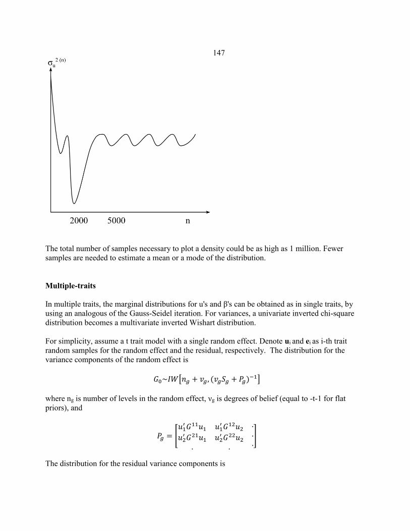
147

The total number of samples necessary to plot a density could be as high as 1 million. Fewer

samples are needed to estimate a mean or a mode of the distribution.

Multiple-traits

In multiple traits, the marginal distributions for u's and β's can be obtained as in single traits, by

using an analogous of the Gauss-Seidel iteration. For variances, a univariate inverted chi-square

distribution becomes a multivariate inverted Wishart distribution.

For simplicity, assume a t trait model with a single random effect. Denote ui and ei as i-th trait

random samples for the random effect and the residual, respectively. The distribution for the

variance components of the random effect is

𝐺0~𝐼𝑊[𝑛𝑔 + 𝑣𝑔, (𝑣𝑔𝑆𝑔 + 𝑃𝑔)−1]

where ng is number of levels in the random effect, νg is degrees of belief (equal to -t-1 for flat

priors), and

𝑃𝑔 = [𝑢1

′ 𝐺11𝑢1

𝑢2′ 𝐺21𝑢1

.

𝑢1′ 𝐺12𝑢2

𝑢2′ 𝐺22𝑢2

.

.

.

.]

The distribution for the residual variance components is

148

𝑅0~𝐼𝑊[𝑛 + 𝑣𝑒 , (𝑣𝑒𝑆𝑒 + 𝑃𝑔𝑒)−1]

where n is the maximum number of records (including missing), νe is degrees of belief (equal to -t-1

for flat priors), and

𝑃𝑒 = [𝑒1

′𝑒1

𝑒2′𝑒1

.

𝑒1′𝑒2

𝑒2′𝑒2

.

.

.

.]

If some records are missing, they are predicted from the distribution

"missing records"| u,β, R,G,"known records"

each round and then used as if they were known. Let subscript m denote quantities associated with

missing traits, and p associated with present traits. The missing records can be predicted as:

ym ~ MVN[E(ym|....),Var(ym|...)]

with

E(ym|...)=Xmβ + Zmu +RmpRpp-1(yp-Xpβ + Zpu)

Var(ym|...)=Rmm-RmpRpp-1Rpm

Convergence properties

The Gibss sampler's convergence is tied to the convergence of the method of Gauss-Seidel, and to

priors. When the corresponding convergence of Gauss-Seidel is slow, the convergence of the Gibbs

sampler will be slow too. One way to increase the convergence speed in multiple traits is to use

block iteration, where samples are generated by block of traits.

The Gibbs sample may diverge with certain priors. For example, uninformative priors for variance

components (ν=0) are often worse than flat priors (ν=-t-1).

Computing implementations

The Gibbs sampler require a large number of rounds. Therefore, its efficiency is quite important. In

the most obvious implementation, the LHS is recreated each round, with procedures to set up the

equations taking perhaps as much as 95% of computing time. Also, memory requirements may be

fairly steep. Several algorithms to cut time and memory are possible although some of them are

hard to implement for complicated models. In all cases, the data can be stored in memory or read by

fast routines.

149

Single trait models

In single traits, when working with variance ratios, only the part of the LHS due to (co)variance

matrices changes. If the part of LHS due to records and the relationship matrices are kept in

memory separately, each equation can be reconstructed by combining these matrices and the current

variance ratios, without recomputing the LHS.

Multiple trait models with same model per trait

In this case, only the structure of the LHS for single trait needs to be stored, and the multiple-trait

LHS is reconstructed dynamically using the current (co)variance matrices, as in the previous case.

If some traits are missing, the data needs to be read every round to recreate the missing traits, but

the LHS is not affected.

Other multiple trait models

In large multitrait models, contribution from relationship matrices can be much larger than

contributions from records because single-trait numerator relationship matrices need to be

duplicated over for all combinations of traits and possible sets of correlated effects. To reduce

storage and computations, only the contributions from records can be stored, and contributions from

pedigrees can be recreated from a single-trait copy of the numerator relationship matrix.

Alternately, the model can be redefined so as to have the same model per trait. For example, let the

model be identical except for different fixed management effect m in the i-th trait:

yi = Ximi+....

Redefine that model so that for each trait management effects from all traits are present:

yi = X1m1i + X2m2i + Ximii ....

and treat the effects as random with (co)variances:

𝑐𝑜𝑣(𝑚𝑗𝑖 , 𝑚𝑘𝑖) = {𝑎 → ∞ 𝑖𝑓 𝑖 = 𝑗 = 𝑘𝑏 → 0 𝑜𝑡ℎ𝑒𝑟𝑤𝑖𝑠𝑒

Variance close to 0 cause an effect to disappear while variance of infinity makes an effect fixed; In

practical implementation, values of a should be very high and b very small but in a range so that

numerical errors can be avoided. Also, the Gibbs sampler need to be modified not to sample

variances of m.

Large models

One possibility with large data is by iteration-on-data by Gauss-Seidel, as discussed in an earlier

chapter. Several copies of the data and relationship files may be needed. Programming may become

quite complicated for complex models but is simple for simple models.

150

General models

Updating MME in linked-list form may be time consuming. Matrices in HASH format are faster to

set up, but they need to be converted to IJA format so that rows of the LHS are available

sequentially. Both creation of the hash matrix for the first time and conversion to the IJA format

take time. Schnyder (1998, personal communication) noticed that, after the first round, the structure

of the matrices in the IJA and HASH does not change; only values change. He suggested the

following algorithm:

a) after the first round, create links to facilitate fast conversion between HASH and IJA structures,

b) before every consecutive round, only zero HASH values but not indices.

In the end, the creation of the LHS can be 2-3 times faster without sacrificing any modeling

flexibility.

151

Ways to reduce the cost of multiple traits

In t traits, the computing costs increase as follows

Approximate Cost

Arithmetic Operations Memory

solutions

iterative

finite

>t2

t3

t2

t2

REML

Derivative-free

Derivative

t5

t3

t2

t2

The cost of obtaining iterative solutions includes the cost of increased number of rounds because of

a lower convergence rate, which is especially low when traits are missing.

Canonical transformation

Let the t-trait model be

𝑦 = 𝑋𝛽 + 𝑍𝑢 + 𝑒

with

𝑉𝑎𝑟(𝑢) = 𝐺0 ⊗ 𝐺, 𝑉𝑎𝑟(𝑒) = 𝑅0 ⊗ 𝐼

where G0 and R0 are the t x t variance-covariance matrices. For individual trait i, the model is

𝑦𝑖 = 𝑋 ∗ 𝛽𝑖 + 𝑍 ∗ 𝑢𝑖 + 𝑒𝑖

where X* and Z* are single-trait design matrices, same for all traits. The covariances between the

traits are

𝐶𝑜𝑣(𝑢𝑖 , 𝑢𝑗) = (𝑔0)𝑖𝑗𝐺, 𝐶𝑜𝑣(𝑒𝑖, 𝑒𝑗) = (𝑟0)𝑖𝑗𝐼

For any symmetric semi-positive-definite G0 and R0 there is a transformation M such that

M G0 M' = D and M R0 M' = I

where D is the diagonal matrix. For each record j, the vector of observation is

(𝑦1𝑗, 𝑦2𝑗 , …., 𝑦𝑡𝑗)

Multiply each vector of observation by M

152

𝑀(𝑦1𝑗, 𝑦2𝑗, …., 𝑦𝑡𝑗) ⟹ (𝑦1𝑗𝑚, 𝑦2𝑗

𝑚 , …., 𝑦𝑡𝑗𝑚)

which for all observations can be written as

𝑦 ⟹ (𝑀 ⊗ 𝐼)𝑦 = 𝑦𝑚

Then, the model becomes

𝑦𝑚 = 𝑋𝛽𝑚 + 𝑍𝑢𝑚 + 𝑒𝑚

with variances

𝑉𝑎𝑟(𝑢𝑚) = 𝐷 ⊗ 𝐺, 𝑉𝑎𝑟(𝑒𝑚) = 𝐼

where the transformed traits are uncorrelated. For each transformed trait i

𝑦𝑖𝑚 = 𝑋 ∗ 𝛽𝑖

𝑚 + 𝑍 ∗ 𝑢𝑖𝑚 + 𝑒𝑖

𝑚

with covariances between the traits

𝐶𝑜𝑣(𝑢𝑖𝑚, 𝑢𝑗

𝑚) = {𝑑𝑖𝑖𝐺, 𝑖𝑓 𝑖 = 𝑗

0 𝐶𝑜𝑣(𝑒𝑖

𝑚, 𝑒𝑗𝑚) = {

1, 𝑖𝑓 𝑖 = 𝑗0

and the mixed model equation for each trait i are

[

𝑋𝑖𝑚′𝑋𝑖

𝑚 𝑋𝑖𝑚′𝑍𝑖

𝑚

𝑍𝑖𝑚′𝑋𝑖

𝑚 𝑍𝑖𝑚′𝑍𝑖

𝑚 +1

𝑑𝑖𝑖𝐺−1] [

�̂�1𝑚

�̂�1𝑚] = [

𝑋𝑖𝑚′𝑦𝑖

𝑚

𝑍𝑖𝑚′𝑦𝑖

𝑚]

Thus, the single-trait equations after the canonical transformation are uncorrelated and can be

solved by single trait procedures. To compute the solutions on the original scale, back transform

𝑢 = (𝑀−1 ⊗ 𝐼)𝑢𝑚

Note that the canonical transformation can be performed only when the following apply:

- same model for all traits

- no missing traits for any observation

- single random effect

The transformation matrix can be constructed as follows. Decompose Ro into eigenvectors and

eigenvalues

𝑅0 = 𝑉𝐷𝑟𝑉′ Then decompose again

153

𝐷𝑟

−12𝑉′𝐺0𝑉𝐷𝑟

−12 = 𝑊𝐷𝑊′

The transformation matrix is

𝑀 = 𝑊′𝐷𝑟

−12 𝑉′

For verification

𝑀𝐺0𝑀′ = 𝑊′𝐷𝑟

−12 𝑉′𝐺0𝑉𝐷𝑟

−12𝑊 = 𝑊′𝑊𝐷𝑊′𝑊 = 𝐷

𝑀𝑅0𝑀′ = 𝑊′𝐷𝑟

−12 𝑉′𝑉𝐷𝑟𝑉′𝑉𝐷𝑟

−12𝑊 = 𝑊𝐷𝑟

−12𝐷𝑟

−12𝑊′ = 𝐼

Canonical transformation and REML

Estimation of REML by canonical transformation can be done by the following steps:

a) Assign priors for R0 and G0

b) Find transformation and transform the data

c) Estimate single-trait variance components

d) Combine the estimates; the formulas below assume the first-derivative algorithm

𝑟𝑖𝑖𝑚 =

𝑦𝑖𝑚′𝑦𝑖

𝑚 − �̂�𝑖𝑚𝑋∗′

𝑦𝑗𝑚 − �̂�𝑖

𝑚𝑍∗′𝑦𝑗

𝑚 +�̂�𝑖

𝑚′𝐺−1�̂�𝑗𝑚

𝑑𝑖𝑖

𝑛𝑟 − 𝑟𝑎𝑛𝑘(𝑋∗) +𝑡𝑟(𝐺−1𝐶𝑚,𝑖)

𝑑𝑖𝑖

𝑟𝑖𝑖𝑚 =

(𝑦𝑖𝑚′𝑦𝑖

𝑚 − �̂�𝑖𝑚𝑋∗′

𝑦𝑗𝑚 − �̂�𝑖

𝑚𝑍∗′𝑦𝑗

𝑚)

𝑛𝑟 𝑓𝑜𝑟 𝑖 ≠ 𝑗

𝑔𝑖𝑖𝑚 =

�̂�𝑖𝑚′𝐺−1�̂�𝑗

𝑚

𝑛𝑔𝑖−

𝑡𝑟(𝐺−1𝐶𝑚,𝑖)𝑑𝑖𝑖

𝑔𝑖𝑖𝑚 =

�̂�𝑖𝑚′𝐺−1�̂�𝑗

𝑚

𝑛𝑔𝑖

where nr is number of records, ng is number of levels in the random effect, and Cm,i is the

block of the inverse of the coefficient matrix corresponding to random effect i. Form

�̂�0𝑚 = {𝑟𝑖𝑗

𝑚}, �̂�0𝑚 = {𝑔𝑖𝑗

𝑚}

The new estimate of (co)variance components on the original scale are

�̂�0 = 𝑀−1�̂�0𝑚𝑀−1′, �̂�0 = 𝑀−1�̂�0

𝑚𝑀−1′

154

e) If no convergence, repeat from b)

Contrary to general model REML, the cost of canonical transformation REML is only linear with

the number of traits, and there is no increase in memory over single-trait. However, all limitations

of the canonical transformation apply.

Numerical properties of canonical transformation

With many traits, some traits are likely to become almost linear functions of the other traits.

Therefore, matrices R0 and G0 may became almost singular, and the whole coefficient matrix can

become almost singular. This can easily be shown for a mixed model. The condition number of a

matrix is defined as

cond(B)=|B| |B-1|

where higher condition numbers are associate with poorer numerical properties. In a general

multiple-trait fixed model, the coefficient matrix is

𝑅0 ⊗ 𝑋′𝑋 with the condition number

𝑐𝑜𝑛𝑑(𝑅0 ⊗ 𝑋′𝑋) = 𝑐𝑜𝑛𝑑(𝑅0) 𝑐𝑜𝑛𝑑(𝑋′𝑋)

Similar increase in condition number occurs in mixed models, where that condition is also a

function of G0 but it is more difficult to show analytically. High condition number of a matrix

leads to numerical errors in the factorization, or to extremely low convergence rate in iterative

methods. In variance component estimation, the computed rank of the coefficient matrix may

change from round to round.

In the canonical transformation, the coefficient matrix in the fixed model is

X'X

and thus its condition is independent on R0.

In canonical transformation, the near singularity R0 and G0 shows in elements of D and Dr being

almost 0. Computer program MTC contains the following heuristics with respect to the canonical

transformation. For the residual eigenvalues:

𝑖𝑓 (𝐷𝑟)𝑖𝑖 = 0 𝑡ℎ𝑒𝑛 𝑠𝑒𝑡 (𝐷𝑟−1)𝑖𝑖 = 0

and for the "random effect eigenvalues":

𝑑𝑖𝑖 = max(0.2, 𝑑𝑖𝑖) , 𝑑𝑖𝑖 = min (𝑑𝑖𝑖, 100,000)

While general-model REML by any algorithm for more than 3-6 traits isn't usually stable

numerically, the canonical transformation REML was known to be successful for 32 traits!

155

Extensions in canonical transformation

Multiple random effects

Extend the model to p multiple random effects

𝑦 = 𝑋𝛽 + ∑𝑍𝑘𝑢𝑘 + 𝑒

𝑘

with

𝑉𝑎𝑟(𝑢𝑘) = 𝐺0𝑘 ⊗ 𝐺𝑘

We need such a transformation that

M R0 M' = I

and

M G0k M' = Dk, k=1, p

where Dk are diagonal matrices. In general, such a transformation does not exist for p>1. Lin and

Smith (4) hypothesized that in practical situations an approximate equation can hold

M G0k M' ≈ Dk

The algorithm to calculate M would be similar as before

𝑅0 = 𝑉𝐷𝑟𝑉′

W and Di in the decomposition

𝐷𝑟−1/2

𝑉′𝐺0𝑖𝑉𝐷𝑟−1/2

= 𝑊𝐷𝑖𝑊′

can be obtained approximately by the FG algorithm (Flury, 1988)

The transformation matrix is

𝑀 = 𝑊′𝐷𝑟−1/2

𝑉′

For a good approximation, matrices G0k must be alike. In general multiple traits with t traits and p

random effects, the total number of parameters to estimate is:

p t (t+1)/2

With the approximation, the number of parameters would be

(p-1) t +t(t+1)/2

For 2 random effects and 4 traits, the number of parameters is 20 in the first case and 14 in the

second case.

156

Misztal et al. (1993) has obtained very good results with the approximation for type and milk traits.

This indicates that the multiple-trait variance-covariance structure in several random effects is

similar. Reversely, in that case, general REML would estimate more parameters than necessary.

Missing traits

Ducrocq and Besbes (1993) have developed a method to apply the canonical transformation when

records on some traits are missing. Let ym be the m-th observation partitioned as (ymα, ymβ), where

ymα was recorded but ymβ is missing. Denote the model for each part as

𝑦𝑚𝛼 = 𝑥𝑚𝛼′ 𝛼 + 𝑧𝑚𝛼

′ 𝑢 + 𝑒𝑚𝛼

𝑦𝑚𝛽 = 𝑥𝑚𝛽′ 𝛽 + 𝑧𝑚𝛽

′ 𝑢 + 𝑒𝑚𝛽

Let (k) denote the current round of iteration. Missing record ymβ can be predicted using the equation

�̂�𝑚𝛽(𝑘)

= 𝑥𝑚𝛽′ 𝛽(𝑘) + 𝑧𝑚𝛽

′ 𝑢(𝑘) + 𝐸(𝑒𝑚𝛽|𝑦𝑚𝛽 , 𝛽(𝑘), 𝑢(𝑘))

= 𝑥𝑚𝛽′ 𝛽(𝑘) + 𝑧𝑚𝛽

′ 𝑢(𝑘) + 𝑅0,𝛽𝛼𝑅0,𝛽𝛼−1 (𝑦𝑚𝛼

(𝑘)−𝑥𝑚𝛼

′ 𝛼(𝑘) + 𝑧𝑚𝛼′ 𝑢(𝑘))

where R0,αβ is a block of R0 corresponding to traits α and β, and R0,αα is a square block of R0

corresponding to trait α.

To solve the mixed model equations, in each round predict missing records and use them for one

round of iteration as if they were known. Then, using the new estimates, predict the missing records

again. Continue until convergence.

Canonical transformation with missing traits requires that in each round the previous round

estimates be untransformed, data read, the missing records predicted, and all the records

transformed.

Formulas to apply the modification for missing records to REML has not been derived. Thus, the

procedure is applicable only for obtaining the solutions.

Different models per trait

When a random effect is absent in one or more traits, one can still define that effect for all traits but

set the variance(s) for these traits very high so that this effect is practically eliminated. If there are

many random effects and the approximate diagonalization is being used, this could have a side

effect of poor diagonalization.

There are two methods to handle different fixed effects per trait. In a simple but approximate

method by Gengler and Misztal (1995), one creates a model containing all fixed effects. Then

157

clusters of traits with identical models are created. Then, such clusters are augmented to all traits by

predicting the missing observations, and the missing-record procedures are applied. The model for

each cluster includes all fixed effects, but effects undesirable in the given cluster are assigned

"dummy" levels. Consider the data

Cow

Fixed effects Traits

Herd-year-

season

Herd-time of

classification Classifier Milk Fat Stature

Udder

width

1 1 1 1 6000 200 30 19

2 2 2 1 7000 225 45 37

3 2 3 2 8000 250 28 43

where herd-year season applied to milk and fat, and heard-time-of-classification applied to stature

and udder width.

The data can be restructured to

Cow


Herd-year-

season

Herd-time of

classification Classifier Milk Fat Stature

Udder

width

1 1 D D 6000 200 M M

2 2 D D 7000 225 M M

3 2 D D 8000 250 M M

1 D 1 1 M M 30 19

2 D 2 1 M M 45 37

3 D 3 2 M M 28 43

where M denotes missing trait and D denotes the dummy effect. For example, if herd year season

had 100 levels, and herd-time-classification had 1000 levels, D=101 for herd-year-season and

D=1001 for herd-time-classification. Because the herd effects do not overlap, they can be joined to

reduce storage

158

Cow


Herd-year-season or Herd-

time of classification Classifier Milk Fat Stature

Udder

width

1 1 D 6000 200 M M

2 2 D 7000 225 M M

3 2 D 8000 250 M M

1 1 1 M M 30 19

2 2 1 M M 45 37

3 3 2 M M 28 43

This method may be an approximation because the residuals of different clusters are assumed

uncorrelated.

Another method was proposed by Ducrocq and Chapuis (1997). Define all effects for all traits. Let

β be solutions to all the fixed effects where all fixed effects are applied to all traits, and let βc be

solutions constrained so that solutions to fixed effects that should be absent for certain traits are 0.

Find such a transformation P so that

βc = Pβ

and then find an equivalent transformation on the canonical transformation side

Solve iteratively using all the fixed effects, and the end of each round apply the above

transformation, either on the original or on the transformed scale.

𝛽𝑚𝑐 = 𝑃𝑚𝛽𝑚

Implicit representation of general multiple-trait equations

Tier and Graser (1991) presented a way to drastically reduce the amount of storage for multiple-trait

mixed model equations. Initially assume that all traits follow the same model but some traits are

missing, and that there is only one random effect. For each missing trait combination i, the mixed

model can be written as

𝑦𝑖 = 𝑊𝑖𝜃 + 𝑒

The left hand side of the mixed point equations can be written as

𝑅0(1)

⊗ 𝑊1′𝑊2 + 𝑅0

(2)⊗ 𝑊2

′𝑊2+. . +𝑅0(𝑞)

⊗ 𝑊𝑞′𝑊𝑞 + 𝐺0

−1 ⊗ 𝐴−1

= 𝑅0(1)

⊗ 𝐶(1) + 𝑅0(2)

⊗ 𝐶(2)+. . +𝑅0(𝑞)

⊗ 𝐶(𝑞) + 𝐺0−1 ⊗ 𝐶(𝑎)

159

where Ro(i) is the inverse of the residual (co)variance matrix for a missing trait combination i. For t

traits, the memory needed to store the coefficient matrix can be close to t2 greater than that for

single traits because scalars in single trait are being expanded to txt blocks.. Each txt block

corresponding to the jk-th single-trait equation can be computed as

𝑅0(1)

𝑐𝑗𝑘(1)

+ 𝑅0(2)

𝑐𝑗𝑘(2)

+. . +𝑅0(𝑞)

𝑐𝑗𝑘(𝑞)

+ 𝐺0−1𝑐𝑗𝑘

(𝑎)

= [𝑐𝑗𝑘(1)

𝑐𝑗𝑘(2)

… 𝑐𝑗𝑘(𝑞)

𝑐𝑗𝑘(𝑎)

]

[ 𝑅0

(1)

𝑅0(2)

…

𝑅0(𝑞)

𝐺0 ]

= 𝑐𝑗𝑘

[ 𝑅0

(1)

𝑅0(2)

…

𝑅0(𝑞)

𝐺0 ]

= 𝑐𝑗𝑘𝑅∗

Instead of storing the complete coefficient matrix, it is sufficient to store C={cjk}. Each vector cjk

contains counts of "kernels", and it has as many elements as there are combinations of missing

effects in the data + 1. In a 5-trait situation, where there are five patterns of missing traits, each txt

block would require the storage of 15 elements, and the corresponding vector c only 6 elements.

The storage requirements can drop further if counts are kept by 2-byte or even 1-byte numbers as

opposed to 4- or 8-byte real numbers for the coefficients.

The method can be further refined if one creates a list of all txt blocks that are present in the

coefficient matrix, and each entry in the coefficient matrix is a pointer to an element in this list.

Example

Consider the model

y = Hh + Za + e

where h is the herd effect, a is the animal effect, and the data is

animal sire dam herd milk protein somatic

cell score

1 4 3 1 10,000 300 300,000

2 4 - 1 12,000 - -

2 4 - 2 13,000 - -

3 - - 2 13,000 350 -

3 - - 2 11,000 - -

4 - - 2

The data contains 3 classes of missing effects:

class missing

1 none

2 somatic cell score

160

3 protein and somatic cell score

The matrix C would contain the following vectors when shown upper-stored

1 0 1 0 1 0 0 0 0 0 1 0

0 1 2 0 0 0 1 0 0 1 1 0

1 0 0 2 0 0 0 -1 0 0 0 -1

0 0 2 1.33 0 0 0 -.66

0 1 1 1.5

0 0 0 1.86

Because many vectors would appear more than once, one can store the matrix C as links and a list.

1 2 3

4 3 5

6 7 7

8 9

10

11

161

list

1 1 0 1 0

2 1 0 0 0

3 0 0 1 0

4 0 1 2 0

5 0 1 1 0

6 1 0 0 2

7 0 0 0 -1

8 0 0 2 1.33

9 0 0 0 -.66

10 0 1 1 1.5

11 0 0 0 1.86

Most likely, only a few elements in the list will occur in most of the entries. Solutions by block

iteration would involve Cholesky decomposition of diagonal blocks cjjR*. Because some of the

blocks can occur many times, computer time may be saved by precomputing the Cholesky

decomposition for all types of blocks on the diagonal of C.

The above technique complicates when models for each trait are different. For special

considerations in such a case, see the work by Tier (1992).

162

Computing in genomic selection

In genomic selection (Meuwissen et al., 2001), animals are genotyped by large panels of SNP,

effects of SNP markers or haplotype segments based on those markers are predicted, and those

predictions are used to estimate genomic breeding values for young animals based on their

genotypes. Commercial genotyping is usually with about 50k SNPs, with special analyses of

sequence-type data involving millions of SNPs.

Common genomic analyzes can be of several types including:

1. Estimation of SNP effects in a model that includes only genotyped animals,

e.g., BayesA, BayesB (Meuwissen et al., 2001).

2. Estimation of breeding values using SNP-derived genomic relationship matrix G for only

genotyped animals (VanRaden, 2008).

3. Regular BLUP where a pedigree relationship matrix has been replaced by combined

pedigree/genomic matrix H (Aguilar et al., 2010; Christensen et al., 2010).

Estimation of SNP effects

Assume a simple model:

y =μ + Za + e

where y are (possibly deregressed) proofs of high reliability animals, a are effects of individual SNP

or haplotype effects, Z is a matrix relating animals to markers; var(a)=Da or Iσ2a, var(e)==De or

Iσ2e; Dx are diagonal matrices. The genomic prediction u of animals based on the predicted effects

is:

�̂� = 𝑍𝑎�̂�

where Za is a matrix relating animals in a to respective SNP or haplotype effects.

In methods like BayesA, solutions to a are obtained by Gauss-Seidel iteration. Due to a large

number of effects, a straightforward implementation of GS leads to a large number of operations.

For example, if there are 500,000 SNP effects in the model, the number of different contributions to

the system of equations resulting from one observation is 500,0002 = 2.5*1011 and the amount of

memory required is > 1000 Gbytes (half storage + double precision).

Efficient Gauss-Seidel with SNP information

Legarra and Misztal (JDS 2008) looked at methods to compute solutions to a. One can avoid large

storage by using the iteration on data. Such iteration with the PCG algorithm is very fast. The

iteration on data using the regular Gauss-Seidel in a straightforward implementation such as below

is very slow (quadratic with the number of SNP:

163

𝑢𝑗 =𝑧𝑗

′[𝑦 − ∑ (𝑧𝑖𝑎)]𝑖,𝑖≠𝑗

𝑧𝑗′𝑧𝑗 + 𝑑𝑗

, 𝑗 = 1, 𝑛

where zi is the i-th a column of Z, aj is the j-th solution and dj is variance ratio for the j-th solution;

for simplification μ has been removed from the model and a on the right side is the most up-to-date

solution. The slowness is due to the large number of effects in the summation: typically about

50,000 rather than a typical 10 in a regular animal model. Janns and de Jong (1999) noticed that:

𝑦 − ∑(𝑧𝑖𝑎) = �̂� +

𝑖,𝑖≠𝑗

𝑧𝑗𝑧𝑎𝑗

Subsequently, the iteration can be implemented much faster as:

𝑢𝑗 =𝑥𝑗

′(�̂� + 𝑥𝑗′𝑥𝑗𝑎𝑗)

𝑧𝑗′𝑧𝑗 + 𝑑𝑗

, 𝑗 = 1, 𝑛

but after computing every solution, the estimated residuals need to be updated:

�̂� = �̂� − 𝑥𝑗 ∆𝑎𝑗 , 𝑗 = 1, 𝑛

where Δuj is the change in the value of uj. The cost of the new iteration is linear with the number of

SNP.

PCG iteration on data

In the PCG iteration, the efficiency with SNP is obtained by avoiding matrix by matrix

multiplication and replacing it by successive matrix by vector operations. The left hand side of a

model with SNP is:

LHS=Z'Z +D-1

The most time-consuming operation in PCG is computing a product of LHS with a vector, say q.

The following avoid the matrix x by matrix operation:

LHS q = (Z'(Zq) +D-1q

Genomic relationship matrix

The model:

y =μ + Za + e; var(a)=D𝜎𝑎2

where D is a diagonal matrix of relative variance for each SNP, is equivalent to

𝑦 = 𝜇 + 𝑢 + 𝑒; 𝑣𝑎𝑟(𝑢) = 𝑍𝐷𝑍′𝜎𝑎2= 𝐺𝜎𝑢

2

164

where G is a genomic relationship matrix. Such a model is called GBLUP. The weights in matrix D

can be made equal (D=I), derived in SNP models, or estimated from within GBLUP. With REML

or BLUP software, GBLUP requires G-1.

Conversion between SNP effects and GEBV

GEBV can be obtained from SNP effects:

𝑢 = 𝑍𝑎

SNP effects can be obtained from GEBV (Stranden and Garrick, 2009):

𝑎 = 𝐷𝑍′𝐺−1𝑢

As a check,

𝑢 = 𝑍𝑎 = 𝑍𝐷𝑍′𝐺−1𝑢 = 𝑢

Conversions enable estimation of weights (and GWAS) in the GBLUP context (e.g., Wang et al.,

2012; Sun et al., 2012).

Joint relationship matrix H and single-step GBLUP

Legarra et al. (2009) presented a relationship matrix that combines A and G into H:

𝐻 = 𝐴 + [𝐴12𝐴22−1 0

0 𝐼] [

𝐼𝐼] [𝐺 − 𝐴][𝐼 𝐼] [

𝐴22−1𝐴12 00 𝐼

]

where index 1 refers to ungenotyped and 2 to genotyped animals. Such a matrix can be used

indirectly, without inversion, in nonsymmetrical BLUP (Misztal et al., 2009). This is accomplished

with PCG by successive multiplication of components of H. A product of A12q can be computed

efficiently using the Colleau et al. (2002) algorithm.

The inverse of H is simpler than H itself (Aguilar et al., 2010, Christensen et al., 2010):

𝐻−1 = 𝐴−1 + [0 00 𝐺−1𝐴22

−1]

and can be used in regular mixed model software. Success with H-1 depends on the ability to

calculate G-1 and A22-1. BLUP with matrix H is called single-step GBLUP or ssGBLUP as it

computes GEBV from phenotypes, pedigree and the genomic information in a single step.

165

Efficiency in computing can be obtained by using 1) parallel processing that utilizes multiple cores

in current computers, 2) specialized libraries that optimize computations for specific computers.

With OpenMP structures for parallel processing and Intel libraries, computing of G-1 and A22-1 for

50,000 animals takes about 1 hr on a 2013 server (Aguilar et al., 2014).

BLUP using H is called single-step GBLUP or ssGBLUP, as opposed to multiple steps when

former procedures like BayesB are involved. Multi-step procedures involve a few approximations:

inaccurate computing of deregressed proofs, assumptions of uncorrelated residuals in BayesB,

approximation in constructing an index that blends parent average with genomic predictions. These

approximations are avoided in ssGBLUP, however, the inappropriate selection of G can result in

biases and deterioration of accuracy. In general, the j-th genotype of animal i zij is calculated as:

2-2pj, when genotype = 11

zij = 1-2pj, when genotype = 10V01

-2pj, when genotype = 0

where pj is j-th allele frequency. See Forni et al. (2010) on effects of different choices for p. When

the average of G is smaller/larger than that of A22, EBV of genotyped animals are biased

downward/upward compared to EBV of the rest of animals (Cheng et al., 2011). Biases can be

avoided if G is computed using current allele frequencies and then adjusted to have averages similar

to A22 ,e.g.:

G=G+avg(offdiag(A22)

The offset above is equivalent to a fixation index FST (Vitezica et al., 2011). If the population is

composed of multiple lines or breeds, G needs to be adjusted separately for each line or breed

combination.

ssGBLUP has been used successfully for large multiple-trait procedures, e.g., for fertility in 3

parities (Aguilar et al., 2011) and 18 type traits (Tsuruta et al., 2011). With careful programming

the running time can be less than twice of regular models with 10k genotypes.

166

Fine tuning

The theory of H makes many assumptions, and many of these many not hold in practice. Several

studies found that better accuracies and lower biases of GEBV can be achieved by adjusting τ and

ω in H defined as below:

𝐻−1 = 𝐴−1 + [0 00 𝜏𝐺−1𝜔𝐴22

−1]

Generally, τ<1 and ω<1. Note that large ω causes H to be close to non-positive definite, causing

slower convergence or even divergence when MME are solved by iteration, while smaller ω will

generally cause better convergence; the effect ω of is due to heterogeneous base populations

(Misztal et al., 2013). One way to improve the convergence rate is to remove old pedigrees or even

old data altogether, especially when the base population is heterogeneous, i.e., parents are missing

across generations (Lourenco et al., 2014).

Large number of genotypes and APY algorithm

When G-1 and A22-1 are computed explicitly, the cost is cubic with the number of genotypes.

Subsequently, costs with > 50-100k genotypes are excessive. However, both inverses can be

calculated indirectly at a greatly reduced cost.

In general, the effective rank of G (after removing noise) is equal to the number of LD blocks (or

independent chromosome segments). If there are m such blocks, GEBV of m random animals

contain complete information on the value of those blocks. Split the population into n core animals

("c") and the remaining non-core animals ("n"). Then,

𝑢𝑛 = 𝑃𝑒 + 𝑒

where Pc relates to noncore animals and e is a small error. Following, in the APY algorithm

(Misztal, 2016):

𝐺−1 = [𝐺𝑐𝑐−1 00 0

] + [𝐺𝑐𝑐−1𝐺𝑐𝑛

𝐼]𝑀−1[−𝐺𝑐𝑛𝐺𝑐𝑐

−1 𝐼]

where M is a diagonal matrix with elements

𝑚𝑖 = 𝑔𝑖𝑖−𝐺𝑛𝑐𝐺𝑐𝑐−1𝐺𝑐𝑛

Only a fraction of G needs to be computed and the inverse is sparse matrix with approximately a

linear cost. In practice, the number of core animals ranges from about 5k in pigs and broiler chicken

to 10-15k in cattle (Pocrnic et al., 2016). Inversion for > 500k genotyped animals take hours

(Masuda et al., 2016). Core animals can be a random sample of all genotyped animals with high

167

quality genotypes. Reliabilities of GEBVs with APY inverse could be 1-3% higher than with a

regular inverse, partly due lower sampling noise from redundant recursions.

While G-1 for a large number of animals is sparse, A22-1 can be dense (Faux and Genegler, 2013).

This matrix can be computed indirectly (Stranden and Mantysaari, 2014):

𝐴22−1 = 𝐴22 − (𝐴12)′(𝐴11)−1(𝐴12)

where all matrices on the right hand side are submatrices of sparse A-1 and can be stored explicitly.

In the PCG algorithm, only a product of a matrix by a vector is needed. Then A22-1q can be

computed as

𝐴22−1𝑞 = 𝐴22𝑞 − (𝐴12)′[(𝐴11)−1[𝐴12𝑞]]

With some exception (solving step with A11), computations include only products of amatrices by a

vector. See (Masuda et al., 2016) for details.

Imputation for nongenotyped animals

Fernando et al. (2014) proposed single-step by imputing genotypes of nongenotyped animals.

Subsequently, their equations involve only SNP effects and do not require creating G explicitly. As

proposed, the algorithm for imputation is very time consuming.

168

Data manipulation

So far we assumed that the data are available in an ordered way, with all effects numbered

consecutively from 1. A substantial part of data analysis is selection of records, data checks and

renumbering.

Renumbering

Data for mixed model programs require consecutive coding. Each effect should be coded from 1 to

the last level, without gaps. One of the more difficult renumbering is for the animal effect.

The purpose of that ordering is:

1. Detection of discrepancies in pedigrees

- parents too young or too old than progenies

- animal as both male and female,

- too many progenies per female

2. Elimination of unnecessary animals

- animals without records and

without progeny, or

with one progeny and no parent

3. Assignment of unknown parent groups (if desired)

4. Actual renumbering in the format

animal code; sire code; dam code; parents' code.

The parents' code tells how many animals have been replaced by unknown parent groups. It is

desirable to code animals with records first because in that case the permanent environmental effect

(in the repeatability model) can share coding with the animal effect.

5. Renumbering the animal id in the performance file. If the maternal effect is present, it needs to be

added to the performance file and a code for missing dams assigned for a record of an animal whose

maternal information is unavailable.

Memory consideration

If one prepares a subset of the data, e.g., for a REML analysis, the number of animals in the

pedigree file can be much larger than the number of animals in the performance file because of

many noncontributing animals. The size of pedigrees can be limited if one considers animals in the

following order:

- animals with records

- parents of above animals

169

- parents of above animals

- .....................................

or from the youngest animal to the oldest. The removal of unnecessary animals can then proceed in

the reverse direction, from the oldest to the youngest.

There are two basic methods of renumbering:

A. by look-up tables

B. by sorting and merging

A. Look-up tables

Pseudo-program

Open performance file

Load all animals with records into memory

Sort pedigree file by year of birth descending

For each pedigree record

If animal in memory, load parents, year of birth, and possibly other info; accumulate # parents and

#progeny

Sort animals in memory by year of birth ascending

For each animal

If noncontributing

Remove,

Eliminate contributions of current animal to parents and progeny

If desired, calculate inbreeding and/or unknown parent groups

Write renumbered pedigree file

Open performance file

For each record

Substitute original animal id by consecutive number

If desired, add inbreeding and/or maternal fields

Write record

For fast search, the "hash" is about the most efficient.

Look-up approach is fast but memory intensive:

10-50 bytes of memory per animal,

10-50 Mbytes per 1 mln animals

B. Sort and merge

1. From pedigree and data files, extract animal id with estimated year of birth and code, which is

one of a) has record, b) has pedigree record, c) has progeny

170

2. Sort by animal id

3. Summarize single entry per animal with:

number of records,

number of parents

number of progeny

4. Remove noncontributing animals

5. Assign consecutive numbers, first to animals with records

6. Sort data file by animal,

7. Sort pedigree file by animal; merge in animal consecutive number

8. Sort pedigree file by dam, merge in dam consecutive number

9. Sort pedigree file by sire; merge in sire consecutive number

Sort and merge renumbering:

need very little memory but plenty of disk space

speed dependent on sorting!

Examples

animal a2 is redundant!

171

animal dam sire year of birth record

a1 a0 - 80 10

a4 a1 a3 85 15

a5 a4 - 90 12

sire pedigree file

bull dam sire year of birth

a2 - - 75

a3 a0 a2 80

Required unknown parent group allocations

year of birth of youngest progeny unknown parent group

<85 1

≥85 2

Contents of look-up table after loading animals with records (order dependent on search algorithm)

animal #parents #progeny #records birth #number

a1 0 0 1 80 1

a4 0 0 1 85 2

a5 0 0 1 90 3

Contents of look-up table after loading parents and parents of parents of animals with records

animal #parents #progeny #records birth #number

a1 1 1 1 80 1

a0 0 2 0 75 4

a4 2 1 1 85 2

a3 2 1 0 80 5

a5 1 0 1 90 3

a2 0 1 0 75 (none)

The last animal is noncontributing and can be eliminated. Renumbering of the pedigree done by one

pass through the pedigree file. Unknown parents initially are assigned the birth year of their oldest

progeny

172

animal dam sire year of birth

1 4 (80) 80

2 1 5 85

3 2 (90) 90

5 4 (80) 80

4 (75) (75) 80 year of birth predicted as year of birth of progeny - 5

Unknown parent groups are replaced by consecutive numbers after the highest animal number, and

the code shows the number of unknown parents

animal dam sire code

1 4 6 1

2 1 5 0

3 2 7 1

5 4 6 1

4 6 6 2

The records' file with animal id and records is created by reading the records file again and merging

the animal id with the animal consecutive number

animal record

1 10

2 15

3 12

173

Sort and Merge approach

First file:

animal type of entry year of birth

a1 record&ped 80

a0 dam 80

a4 record&ped 85

a1 dam 85

a3 sire 85

a5 record&ped 90

a4 dam 90

a2 sire_ped 75

a3 sire_ped 80

a0 dam 80

a2 sire 80

After sorting by type of entry within animal:

(rec = record. pedx = pedigree record with x known parents)

a0 dam 80

a0 dam 80

a1 dam 85

a1 rec&ped1 80

a2 sire 80

a2 sire_ped0 75

a3 sire 85

a3 sire_ped1 80

a4 dam 90

a4 reco&ped2 85

a5 rec&ped1 90

At this point entries can be read and analyzed, one animal at a time.

The renumber file would first be constructed with negative numbers for animals without records,

because the maximum number of animals with records is not known until the file end:

animal #consecutive

a0 -1

a1 1

a3 -2

a4 2

a5 3

and in another pass, the same animals with records will have consecutive numbers corrected:

174

animal #consecutive

a0 4

a1 1

a3 5

a4 2

a5 3

The cow file is sorted by animal and merged with the animal file. The result is the data file:

animal record

1 10

2 15

3 12

and pedigree files:

1 a0 (80) (80) means unknown with animal born in 1980!

2 a1 a3

3 a4 (90)

The sire pedigree file is sorted by sire, merged with the animal file, and added to the previous

pedigree file:

1 a0 (80)

2 a1 a3

3 a4 (90)

5 a0 a2

Then the file is sorted and merged, first for dam, second for sire:

1 4 (80)

2 1 5

3 5 (90)

5 4 (80)

After that, pedigree entries are added for animals without pedigree records (a0):

1 4 (80)

2 1 5

3 5 (90)

5 4 (80)

4 (80) (80)

Finally, unknown parents are replaced by unknown parent groups. In this case, born before 1985 are

assigned to group 6, the remaining animals assigned to group 7:

1 4 6

175

2 1 5

3 5 7

5 4 6

4 6 6

176

Tools for data manipulation

A look-up approach requires a special program. Such a program is likely to be very fast but can be

quite complicated because of a large number of details. On the contrary, a sort-and-merge type

program can utilize some standard programs and therefore it could be easier to program although

the CPU time would likely to be higher. CPU time is not always important if the program is run

seldomly. What counts is cost of writing the program and ease of modification, which is directly

related to program's complexity.

In pedigree numbering the following standard operations ("primitives") would be almost sufficient:

1. Select records from a file based on conditions

2. Select fields from a file with many fields

3. Sort based on one or more keys

4. Join two or more files

5. Retain unique records (or delete duplicate records)

6. Merge (concatenate) two or more files

7. Number records consecutively

Consider the following data

file ped

animal dam sire code

1 4 6 1

2 1 5 0

3 2 7 1

5 4 6 1

4 6 6 2

file rec

animal record

1 10

2 15

3 12

Create a new file recm that contains all fields from rec and field dam from ped so that the data can

be analyzed with the maternal effect. In the most abstract way, this can be specified as

select animal, record, dam from ped,rec store in recm (1)

Alternatively, using the primitives

sort ped by animal into peds (2)

sort rec by animal into recs

177

join rec and ped by animal into recsm

select animal record dam from recsm into recmat

delete files peds, recs, recsm

The pseudo-programs above assume that the "system" knows names of fields in file. If the system

knows the consecutive numbers of fields only, the same program would be

sort ped by 1 into peds (3)

sort rec by 1 into recs

join rec by 1 and ped by 1 into recsm

select 1 2 4 from recsm into recmat

delete files peds, recs, recsm

If one needs to specify formats for each file separately, then the length of the program increases

drastically and so does the chance of programming errors. For example, the line

sort ped by 1 into peds

could be equivalent to

infile ped (4)

outfile peds

input

animal 1-10

dam 11-20

sire 21-30

code 31

sort by animal

Please note that a change in the format in one file may require corresponding changes in many other

files.

Data manipulation options

Command in pseudo-program (1) would be typical for better databases (Mattison, 1993). In a

database, each file is defined only once. Therefore the chance of making a mistake is greatly

reduced. By using a high definition data manipulation language, e.g., SQL, details of internal

computations need not be specified. Commercial databases may be expensive and require a good

deal of knowledge to operate smoothly. Some elements of the database are present in SAS.

Commands in (3) can be emulated by Unix utilities.

Unix/Linux/MacOS utilities

Let fields in a file be separated by spaces.

178

The sort command works as

sort f1 -o f2

or sort f1 >f2

sorts file f1 to f2 by all fields starting from the first one. The option -o allows for the same input and

output file. Other options allow to sort by multiple keys and in a reverse order

sort +3 -4 +1 -2 -r f1 -o f2

sorts by fields 4 (skip 3 end at 4) and 2 (skip 1 end at 2) in the reverse order (-r). The sort utility can

also be used to merge sorted files, and to test whether a file is sorted.

Repeated fields can be removed by the uniq command

uniq f1 >f2

An option -c prints not only the unique records but also counts of repeated lines.

Command join joins two files based on selection criteria and retains only specified fields

join -j1 1 -j2 4 -o 1.5 1.6 2.3 2.4 f1 f2 >f3

joins files f1 and f2 into f3 based on field 1 in f1 and field 4 in file 2. File f3 contains fields 5 and 6

from file f1 and fields 3 and 4 from file 2.

A selection of fields and records can be done using AWK (GAWK, NAWK). The command

awk '$1>125' f1 >f2

selects records from f1 where the field 1 is greater than 125. Conditions may be more complicated

awk '$1>125 && $2!="" || $1==0' f1 >f2

where either filed 1 is greater than 125 and filed 2 not blank, or field one is zero. Another variant of

awk

awk '{print $1,$5,$6}' f1 >f2

selects only fields 1, 5 and 6 from file f1. There are many special variables in AWK. NR denotes

the consecutive record number, and $0 denotes the complete record. Thus

awk '{print NR, $0}' f1 >f2

precedes each record with its consecutive number. The two variants of AWK can be used together.

179

awk ' $5 == "May" {print $3, $4}' f1 >f2

AWK is also a general programming language that can be used for tasks much more complicated

than shown above. Books on Unix utilities including AWK are available, e.g., Swartz (1990).

The utilities use space as a standard delimiter between fields. If ID's contain spaces, the utilities

have options for other delimiters, e.g., ":".

Perl is a tool more general that awk. It contains constructs like built-in hash storage. There are

reports of Perl being successful in pedigree preparation large national populations.

180

Sources and References

Aguilar, I., and I. Misztal. 2008. Recursive algorithm for inbreeding coefficients assuming non-zero

inbreeding of unknown parents. J. Dairy Sci. 91:1669-1672.

Aguilar, I., I. Misztal, D. L. Johnson, A. Legarra, S. Tsuruta, and T. J. Lawlor. 2010. A unified

approach to utilize phenotypic, full pedigree, and genomic information for genetic evaluation of

Holstein final score. J. Dairy Sci. 93:743:752.

Aguilar, I., I. Misztal , A. Legarra , S.Tsuruta. 2011. Efficient computation of genomic relationship

matrix and other matrices used in single-step evaluation. J. Anim. Breed. Genet. DOI:

10.1111/j.1439-0388.2010.00912.x.

Aguilar, I., I. Misztal, S. Tsuruta, G. R. Wiggans and T. J. Lawlor. 2011. Multiple trait genomic

evaluation of conception rate in Holsteins. J. Dairy Sci. 94:2621-2624.

Aguilar, I., I. Misztal, S. Tsuruta, A. Legarra, and H. Wang. 2014. PREGSF90 - POSTGSF90:

Computational tools for the implementation of single-step genomic selection and genome-wide

association with ungenotyped individuals in BLUPF90 programs. Proc. 10th World Congress Gen.

Appl. Livest. Prod., Vancouver, Canada.

Bazaraa, M.S.; Sherali H. D.; Shetty C.M., 1993: Nonlinear programming. John Wiley & Sons,

New York

Berger, P. J., G. R. Luecke, and A. Hoekstra. 1989. Iterative algorithms for solving mixed model

equations. J. Dairy Sci. 72:514-522.

Boldman, K.G.; Kriese, L. A.; Van Vleck, L. D.; Kachman, S. D., 1993: A manual for use of

MTDFREML. USDA-ARS, Clay Center, Nebraska.

Cantet, R.J.C., and A.N. Birchmeier. 1998. The effects of sampling selected data on Method R

estimates of h2. Proc. World Cong. Genet. Appl. Livest. Prod. 25:529.

Chen, C. Y., I. Misztal, I. Aguilar, S. Tsuruta, T. H. E. Meuwissen, S. E. Aggrey, T. Wing, and W.

M. Muir. 2011. Genome-wide marker-assisted selection combining all pedigree phenotypic

information with genotypic data in one step: an example using broiler chickens. J. Animal Sci.

89:23-28.

Chen, C. Y., I. Misztal, I. Aguilar, A. Legarra, and B. Muir. 2011. Effect of different genomic

relationship matrix on accuracy and scale. J. Anim. Sci. (accepted)

Christensen, O. F. and M. F. Lund. 2010. Genomic prediction when some animals are not

genotyped. Genetics Selection Evolution 42, 2.

181

Colleau, J. J. 2002. An indirect approach to the extensive calculation of relationship coefficients.

Genet. Sel. Evol. 34 (4):409-421.

Druet, T., I. Misztal, M. Duangjinda, A. Reverter, and N. Gengler. 2001. Estimation of genetic

covariances with Method R. J. Anim. Sci. 79:605-615.

Duangjinda, M., I. Misztal, J. K. Bertrand, and S. Tsuruta. 2001. The empirical bias of estimates by

restricted maximum likelihood, Bayesian method, and Method R under selection for additive,

maternal, and dominance models. J. Animal Sci. 2991:2996.

Ducrocq V, Besbes, N. 1993. Solution of multiple-trait animal models with missing data on some

traits. J. Anim. Breed. Genet. 110:81-92.

Ducrocq V, Chapuis, H. 1997. Generalizing the use of the canonical transformation for the solution

of multivariate mixed model equations. Genet Sel Evol. 29:205-224.

Duff IS, Erisman AM, Reid JK 1989 Direct Methods for Sparse Matrices, Clarendon Press, Oxford,

England.

Faux, P., and N. Gengler. 2013. Inversion of a part of the numerator relationship matrix using

pedigree information. Genet. Sel. Evol. 45:45.

Fernando RL, Dekkers JCM and Garrick DJ 2014. A class of Bayesian methods to combine large

numbers of genotyped and non-genotyped animals for whole-genome analyses. Genetics Selection

Evolution 46, 50.

Flury N. 1988. Common Pricipal Components and Related Multivariate Models. John Wiley &

Sons, New York, NY.

Fragomeni, B. O., I. Misztal, D.A.L. Lourenco, S. Tsuruta, Y. Masuda, and T. J. Lawlor. 2014. Use

of Genomic Recursions and Algorithm for Proven and Young Animals for Single-Step Genomic

BLUP Analyses with a Large Number of Genotypes. Proc. 10th World Congress Gen. Appl. Livest.

Prod., Vancouver, Canada.

Forni, S., I. Aguilar, and I. Misztal. 2011. Different genomic relationship matrices for single-step

analysis using phenotypic, pedigree and genomic information. Genet. Sel. Evol. 43:1.

Garrick, D. J., Taylor, J. F. & Fernando, R. L. (2009). Deregressing estimated breeding values and

weighting information for genomic regression analyses. Genetics Selection Evolution 41, 55.

Geman, D., Geman, S. 1991. Bayesian image-restoration, with 2 applications in spatial statistics -

discussion. Ann. I Stat. Math. 43: (1) 21-22.

Gengler, N., and I. Misztal. 1996. Approximation of reliability for multiple-trait animal models

with missing data. J. Dairy Sci. 79:317:328.

182

Groeneveld, E., and Kovacs, M. 1990. A generalized computing procedure for setting up and

solving mixed model equations. J. Dairy Sci. 73:513.

Hayes, B. J., Vissher, P. M. & Goddard, M. E. (2009). Increased accuracy of artificial selection by

using the realized relationship matrix. Genetics Research 91, 47-60.

Hoeschele I. 1997. STAT 5554 Variance Components. Class notes, Virginia Polytechnic Insitute,

Blacksburg.

Höschele I, VanRaden P.M., 1991. Rapid inversion of dominance relationship matrices for

noninbred populations by including sire by dam subclass effects. J. Dairy Sci. 74:557.

Jensen, J., E.A. Mantysaari, P. Madsen and R. Thompson. 1996-7. Residual maximum likelihood

estimation of (co)variance components in multivariate mixed linear models using Average

Information. J. Indian Soc. Ag. Statistics 215:236.

Kaiser, C. J., and B.L. Golden. 1994. Heritability estimation and breeding value prediction using

selected data. J. Anim. Sci.72 (Suppl. 1):147(Abstr.)

Kovac, M. 1992. Derivative Free Methods in Covariance Component Estimation. Ph.D. diss.,

University of Illinois, Urbana.

Laird, N. M.; Lange, N.; Stram D., 1987: Maximum likelihood computations with repeated

measures: application of the EM algorithm. J. American Stat. Associ. 82:97.

Lourenco, D. A. L., I. Misztal, S. Tsuruta, I. Aguilar, T. J. Lawlor, S. Forni, and J. I. Weller. 2014.

Are evaluations on young genotyped animals benefiting from the past generations? J. Dairy Sci.

Legarra, A., and I. Misztal. 2008. Computing strategies in genome-wide selection. J. Dairy Sci.

91:360-366.

Legarra, A., I. Aguilar, and I. Misztal. 2009. A relationship matrix including full pedigree and

genomic information. J. Dairy Sci. 92:4656-4663

Legarra, A., and V. Ducrocq. 2012. Computational strategies for national integration of phenotypic,

genomic, and pedigree data in a single-step best linear unbiased prediction. J. Dairy Sci. 95:4629–

4645.

Lidauer, M., I. Strandén, E. A. Mäntysaari, J. Pösö, and A. Kettunen. 1999. Solving Large Test-Day

Models by Iteration on Data and Preconditioned Conjugate Gradient

J. Dairy Sci. 82:2788-2796.

Lin, C. Y., and S. P. Smith. 1990. Transformation of multitrait to unitrait mixed model analysis of

data with multiple random effects. J. Dairy Sci. 73:2494.

Little RJA, Rubin DB. 1987. Statistical Analysis with Missing Data.

183

Mäntysaari, E. A. and Van Vleck L. D. 1989. Restricted maximum likelihood estimates of variance

components from multitrait sire models with large number of fixed effects. J. Anim. Breed. Genet.

106:409-422.

Mallinckrodt C., B. L. Golden, and A. Reverter. 1996. Confidence Interval for Heritability from

Method R estimates. J. Anim. Sci.74 Suppl. 1:114(Abstr.)

Masuda, Y., I. Misztal, S. Tsuruta, A. Legarra, I. Aguilar, D. Lourenco, B. Fragomeni and T. L.

Lawlor. 2016. Implementation of genomic recursions in single-step genomic BLUP for US

Holsteins with a large number of genotyped animals. J. Dairy Sci. 99:1968-1974.

Mattison RM. 1993. Understanding database management systems: an insider's guide to

architectures, products and design. McGraw-Hill, Inc.

Meuwissen, T. H. E., Hayes, B. J. & Goddard, M. E. (2001). Prediction of total genetic value using

genome-wide dense marker maps. Genetics 157, 1819-1829.

Meurant, G. 1999. Computer solution of large linear systems. Elsevier.

Minoux, M. 1986: Mathematical programming. John Wiley & Sons, Chichester.

Misztal, I., and M. Perez-Enciso. 1993. Sparse matrix inversion in Restricted Maximum Likelihood

estimation of variance components by Expectation-Maximization. J. Dairy Sci. 76:1479.

Misztal, I., T.J. Lawlor, and K. Weigel. 1995. Approximation of estimates of (co) variance

components with multiple-trait Restricted Maximum Likelihood by maximum diagonalization for

more than one random effect. J. Dairy Sci. 78:1862-1872

Misztal, I. 1997. Estimation of variance components with large-scale dominance models. J. Dairy

Sci. 80:965-974.

Misztal, I., T. J. Lawlor, and R.L. Fernando. 1997. Studies on dominance models by Method R for

stature of Holsteins. J. Dairy Sci. 80:975-978.

Misztal, I., A. Legarra, and I. Aguilar. 2009. Computing procedures for genetic evaluation

including phenotypic, full pedigree and genomic information. J. Dairy Sci. 92:4648-4655.

Misztal, I., Z.G. Vitezica, A. Legarra, I. Aguilar, and A.A. Swan. 2013. Unknown-parent groups in

single-step genomic evaluation. J. Anim. Breed. Genet. 130:252–258.

Misztal, I., A. Legarra, and I. Aguilar. 2014. Using recursion to compute the inverse of the genomic

relationship matrix. J. Dairy Sci.

Misztal, I., 2016 Inexpensive computation of the inverse of the genomic relationship matrix in

populations with small effective population size. Genetics 202: 401–409

184

Moré JJ, Wright SJ. 1993. Optimization Software Guide. Society for Industrial and Applied

Mathematics, Philadephia.

Mrode RA 1996. Linear Models For the Prediction of Breeding Values. CAB International,

Wallingford, UK.

Pocrnic, I., D. A. L. Lourenco, Y. Masuda, and I. Misztal. 2016. The Dimensionality of Genomic

Information and its Effect on Genomic Prediction. Genetics. DOI: 10.1534/genetics.116.187013

Press HP, Teukolsky SA, Vetterling WT, Flannery BP. 1996. Numerical Recipees in Fortran 77.

Cambridge University Press, Cambridge, UK.

Press HP, Teukolsky SA, Vetterling WT, Flannery BP. 1996 Numerical Recipees in Fortran 90.

Cambridge University Press, Cambridge, UK.

Reverter A., B. L. Golden, and R. M. Bourdon, 1994. Method R variance components procedure:

application on the simple breeding value model. J. Anim. Sci. 72:2247.

Schaeffer, L. R. 1979. Estimation of variance and covariance components for average daily gain

and backfat thickness in swine. Page 123 in Proc. Conf. in Honor of C. R. Henderson on variance

Components Anim. Breed.

Snelling, W. M. 1994. Genetic analyses of stayability measures of beef females. Ph.D. Diss.,

Colorado State Univ., Fort Collins.

Stranden, I. & Garrick, D. J. (2009). Technical note: Derivation of equivalent computing algorithms

for genomic predictions and reliabilities of animal merit. J. Dairy Sci. 92:2971–2975.

Sun, X., L. Qu, D. J. Garrick, J. C. M. Dekkers, and R. L. Fernando, 2012 A fast EM algorithm for

BayesA-like prediction of genomic breeding values. PLoS One 7: e49157.

Swartz R. 1990. Unix applications programming: mastering the shell. Sams, Carmel, IN.

Tier B. 1992. Factoring common terms in the mixed model equations. J Anim Breed Genet 109:81-

89.

Tier B, Graser HU. 1991. Predicting breeding values using an implicit representation of the mixed

model equations for a multiple trait animal model. J Anim Breed Genet 108:81-88.

Tsuruta, S., I. Aguilar, I. Misztal, and T. J. Lawlor. 2011. Multiple-trait genomic evaluation of

linear type traits using genomic and phenotypic data in US Holsteins. J. Dairy Sci. (accepted)

VanRaden P.M., Höschele I., 1991. Rapid inversion of additive by additive relationship matrices

for noninbred populations by including sire-dam combination effects. J. Dairy Sci. 74:570.

185

VanRaden, P. M. (2008). Efficient methods to compute genomic predictions. Journal of Dairy

Science 91, 4414-4423.

VanRaden, P. M., Van Tassell, C. P., Wiggans, G. R., Sonstegard, T. S., Schnabel, R. D., Taylor,

J.F. & Schenkel F.S. (2009a). Invited review: Reliability of genomic predictions for North

American Holstein bulls. Journal of Dairy Science 92, 16-24.

VanVleck, D. and D.J. Dwyer. 1985. Successive Overrelaxation, Block Iteration, and Method of

Conjugate Gradients for Solving Equations for Multiple Trait Evaluation of Sires. Journal of Dairy

Science 68, 760-767.

Vitezica, Z. G., I. Aguilar, I. Misztal, and A. Legarra. Bias in Genomic Predictions for Populations

Under Selection. Genet. Res. Camb. 93:357–366.

Wade, K. M., and R. L. Quaas. 1993. Solutions to a system of equations involving a first-order

autoregressive process. J. Dairy Sci. 76:3026:3032.

Wang CS, Rutledge JJ, Gianola D. 1993. Marginal inferences about variance components in a

mixed linear model using Gibbs sampling. Genet. Sel. Evolut. 25:41-62

Wang, H., I. Misztal, I. Aguilar, A. Legarra, and W. M. Muir, 2012 Genome-wide association

mapping including phenotypes from relatives without genotypes. Genet. Res. 94: 73–83.

Computational techniques in animal breeding

Documents

Transcript of Computational techniques in animal breeding