Computational Stochastic Optimization: Bridging communities October 25, 2012 Warren Powell CASTLE...
41
Computational Stochastic Optimiz Bridging communities October 25, 2012 Warren Powell CASTLE Laboratory Princeton University http:// www.castlelab.princeton.edu © 2012 Warren B. Powell, Princeton University © 2012 Warren B. Powell
-
Upload
arabella-bell -
Category
Documents
-
view
215 -
download
0
Transcript of Computational Stochastic Optimization: Bridging communities October 25, 2012 Warren Powell CASTLE...

Computational Stochastic Optimization:Bridging communities
October 25, 2012
Warren PowellCASTLE Laboratory
Princeton Universityhttp://www.castlelab.princeton.edu
© 2012 Warren B. Powell, Princeton University © 2012 Warren B. Powell

Outline
From stochastic search to dynamic programming
From dynamic programming to stochastic programming
© 2012 Warren B. Powell

From stochastic search to DP
Classical stochastic search» The prototypical stochastic search problem is posed as
where x is a deterministic parameter, and W is a random variable.
» Variations:• Expectation cannot be computed• Function evaluations may be expensive• Random noise may be heavy-tailed (e.g. rare events)• Function F may or may not be differentiable.
min ( , )x F x WE
© 2012 Warren B. Powell

From stochastic search to DP
Imagine if our policy is given by
Instead of estimating the value of being in a state, what if we tune to get the best performance?
» This is known as policy search. It builds on classical fields such as stochastic search and simulation-optimization.
» Very stable, but it is generally limited to problems with a much smaller number of parameters.
0
min ( , ) , ( | )T
tt t
t
F W C S X S
E E
( | ) arg min ( , ) ( ( , ))n n xt x t f t t
f
X S C S x S S x
© 2012 Warren B. Powell

From stochastic search to DP
The next slide illustrate experiments on a simple battery storage problem.
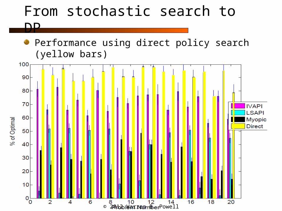
We developed 20 benchmark problems which we could solve optimally using classical methods from the MDP literature.
We then compared four policies:» A myopic policy (which did not store energy)» Two policies that use Bellman error minimization:
• LSAPI – Least squares, approximate policy iteration• IVAPI – This is LSAPI but using instrumental variables
» Direct – Here we use the same policy as LSAPI, but use directly policy search to find the regression vector.
© 2012 Warren B. Powell
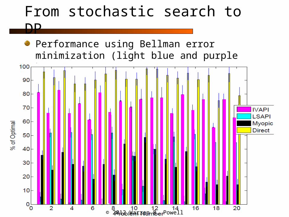
From stochastic search to DP
Performance using Bellman error minimization (light blue and purple bars)
© 2012 Warren B. Powell

Optimal learning
Now assume we have five choices, with uncertainty in our belief about how well each one will perform.
If you can make one measurement, which would you measure?
1 2 3 4 5
Possible values of ( , )store withdrawx
© 2012 Warren B. Powell

Optimal learning
Policy search process:» Choose » Simulate the policy to get a noisy estimate of its value:
WithdrawStore
0
( , ( )) ( ), ( ( ) | ) T
tt t
t
F W C S X S
and store withdraw
© 2012 Warren B. Powell
“a sample path”
( , ( ))F W

Optimal learning
At first, we believe that
But we measure alternative x and observe
Our beliefs change:
Thus, our beliefs about the rewards are gradually improved over measurements
0 0~ ,1x x xN
1 0
0 0 11
0
1 1~ ,1
Wx x
Wx x x
x Wx
x x x
y
N
1 ( , ( )) ~ ,1 Wx xy F W N
i j0x
i j1xW
i j
0x
1x
© 2012 Warren B. Powell

Optimal learning
1 2 3 4 5
No improvement
Now assume we have five choices, with uncertainty in our belief about how well each one will perform.
If you can make one measurement, which would you measure?
© 2012 Warren B. Powell

Optimal learning
1 2 3 4 5
New solution
The value of learning is that it may change your decision.
Now assume we have five choices, with uncertainty in our belief about how well each one will perform.
If you can make one measurement, which would you measure?
© 2012 Warren B. Powell

Optimal learning
An important problem class involves correlated beliefs – measuring one alternative tells us something other alternatives.
1 2 3 4 5
...these beliefs change too.measurehere...
© 2012 Warren B. Powell

Optimal learning with a physical state
The knowledge gradient» The knowledge gradient is the expected value of a single
measurement x, given by
» Knowledge gradient policy chooses the measurement with the highest marginal value.
, 1max ( , ( )) max ( , )KG n n n nx y yE F y K x F y K
Knowledge stateImplementation decision
Updated knowledge state given measurement x
Expectation over different measurement outcomes
Marginal value of measuring x (the knowledge gradient)
Optimization problem given what we knowNew optimization problem
© 2012 Warren B. Powell

The knowledge gradient
Computing the knowledge gradient for Gaussian beliefs» The change in variance can be found to be
» Next compute the normalized influence:
» Let
» Knowledge gradient is computed using
2, 1
2, 2, 1
|n n n nx x x
n nx x
Var K
' 'maxn nn x x x xx n
x
( ) ( ) ( ) ( ) Cumulative standard normal distribution
( ) Standard normal density
f
KG n nx x xf
0
Comparison to other alternatives
© 2012 Warren B. Powell

After four measurements:
» Whenever we measure at a point, the value of another measurement at the same point goes down. The knowledge gradient guides us to measuring areas of high uncertainty.
Optimizing storage
MeasurementValue of another measurement at same location.
Estimated value Knowledge gradient
New optimum
© 2012 Warren B. Powell

Optimizing storage
After five measurements:
Estimated value Knowledge gradient
After measurement
© 2012 Warren B. Powell

Optimizing storage
After six samples
Estimated value Knowledge gradient
© 2012 Warren B. Powell

Optimizing storage
After seven samples
Estimated value Knowledge gradient
© 2012 Warren B. Powell

Optimizing storage
After eight samples
Estimated value Knowledge gradient
© 2012 Warren B. Powell

Optimizing storage
After nine samples
Estimated value Knowledge gradient
© 2012 Warren B. Powell
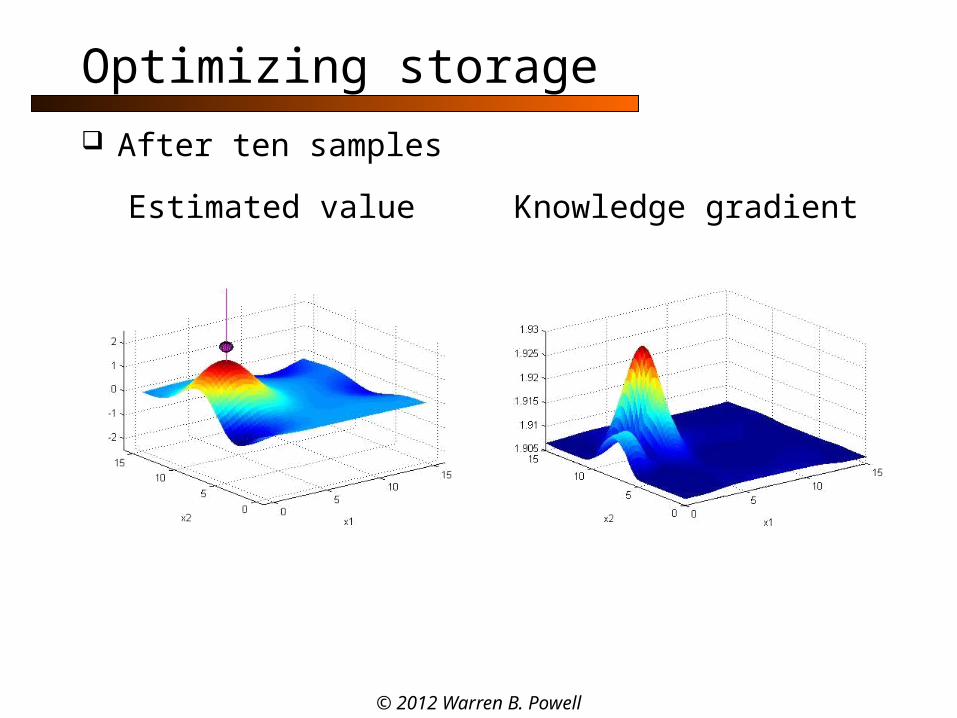
Optimizing storage
After ten samples
Estimated value Knowledge gradient
© 2012 Warren B. Powell

After ten samples, our estimate of the surface:
Optimizing storage
Estimated value True value
© 2012 Warren B. Powell
From stochastic search to DP
Performance using direct policy search (yellow bars)
© 2012 Warren B. Powell

From stochastic search to DP
Notes:» Direct policy research can be used to tune the
parameters of any policy:• The horizon for a deterministic lookahead policy• The sampling strategy when using a stochastic lookahead
policy• The parameters of a parametric policy function approximation
» But, there are some real limitations.• It can be very difficult obtaining gradients of the objective
function with respect to the tunable parameters.• It is very hard to do derivative-free stochastic search with large
numbers of parameters.• This limits our ability to handle time-dependent policies.
© 2012 Warren B. Powell

Outline
From stochastic search to dynamic programming
From dynamic programming to stochastic programming
© 2012 Warren B. Powell

From DP to stochastic programming
The slides that follow start from the most familiar form of Bellman’s optimality equation for discrete states and actions.
We then create a bridge to classical formulations used in stochastic programming.
Along the way, we show that stochastic programming is actually a lookahead policy, and solves a reduced dynamic program over a shorter horizon and a restricted representation of the random outcomes.
© 2012 Warren B. Powell

From DP to stochastic programming
All dynamic programming starts with Bellman’s equation:
All problems in stochastic programming are time-dependent, we write it as
We cannot compute the one-step transition matrix, so we first replace it with the expectation form:
'
( ) min ( , ) ( ' | , ) ( ')as
V s C s a p s s a V s
1 1( ) min ( , ) ( ) |t t a t t t tV S C S a V S S E
1
1 1( ) min ( , ) ( | , ) ( )t
t t a t t t t tS
V S C S a p S S a V S
© 2012 Warren B. Powell

From DP to stochastic programming
Implicit in the value function is an assumption that we are following an optimal policy. We are going to temporarily assume that we are following a fixed policy
We cannot compute the expectation, so we replace it with a Monte Carlo sample. We use this opportunity to make the transition from discrete actions a to vectors x.
( )t tA S
'' ' '
' 1
( ) min ( , ) ( , ( )) |t t
Tt t
t t a A t t t t t tt t
V S C S a C S A S S
E
'' ' '
ˆ ' 1
1( ) min ( , ) ( ), ( ( ))
ˆt t
Tt t
t t x X t t t t tt t
V S C S x C S X S
© 2012 Warren B. Powell

From DP to stochastic programming
The state consists of two components: » The resource vector that is determined by the prior
decisions » The exogenous information . In stochastic
programming, it is common to represent exogenous information as the entire history (starting at time t) which we might write as
While we can always write , in most applications is lower dimensional.
» We will write , where we mean that has the same information content as .
'ttS
'ttR, ' 1,...,tt t tx x
'ttI
' , 1 , ', ,...,tt t t t t th S W W
' 'tt ttI h'ttI
' ' ' ' '( , ) ( , )tt tt tt tt ttS R h R I
'ttI 'tth
© 2012 Warren B. Powell

From DP to stochastic programming
We are now going to drop the reference to the generic policy, and instead reference the decision vector indexed by the history (alternatively, the node in the scenario tree).» Note that this is equivalent to a lookup table
representation using simulated histories.» We write this in the form of a policy, and also make the
transition to the horizon t,…,t+H
Here, is a vector over all histories . This is a lookahead policy, which optimizes the lookahead model.
' '( )tt ttx h'tth
, 1 ,
'' ' ',..., ˆ ' 1
1( ) arg min ( , ) min ( ), ( ( ))
ˆt tt t t t H
t Ht t
t t x X t t tt tt ttx xt t
X S C S x C S x h
, 't tx 'tth
© 2012 Warren B. Powell

From DP to stochastic programming
We make one last tweak to get it into a more compact form:
» In this formulation, we let
» We are now writing a vector for each sample path in . This introduces a complication that we did not encounter when we indexed each decision by a history. We are now letting the decision “see” the future.
, ,
'' '
,..., ˆ '
1( ) arg min ( ), ( )
ˆt t t t H
t Ht t
t t tt ttx x
t t
X S C S x
' , ' ,,..., ( ),..., ( ) ,tt t t H tt t t H tx x x x
t
' ( )ttx
' ( )ttx
© 2012 Warren B. Powell

From DP to stochastic programming
When we indexed by histories, there might be one history at time t (since this is where we are starting), 10 histories for time t+1 and 100 histories for time t+2, giving us 111 vectors to determine.
When we have a vector for each sample path, then we have 100 vectors for each time t, t+1 and t+2, giving us 300 vectors.
When we index on the sample path, we are effectively letting the decision “see” the entire sample path.
© 2012 Warren B. Powell

From DP to stochastic programming
To avoid the problem of letting a decision see into the future, we create sets of all the sample paths with the same history:
We now require that all decisions with the same history be the same:
» These are known in stochastic programming as nonanticipativity constraints.
' ' , 1 ' '( ) | , ( ),..., ( )tt tt t t t tt tth S W W h H
' ' ' ' '( ) ( ) 0 for all ( )tt tt tt tt ttx x h h H
© 2012 Warren B. Powell

From DP to stochastic programming
A scenario tree» A node in the scenario tree is equivalent to a history
t 't
'tth
' '( )tt tthH
1
2
4
3
5
© 2012 Warren B. Powell

From DP to stochastic programming
This is a lookahead policy that solves the lookahead model directly, by optimizing over all decisions over all time periods at the same time. Not surprisingly, this can be computationally demanding.
The lookahead model is, first and foremost, a dynamic program (although simpler than the original dynamic program), and can be solved using Bellman’s equation (but exploiting convexity).
© 2012 Warren B. Powell

From DP to stochastic programming
We are going to start with Bellman’s equation as it is used in the stochastic programming community (e.g. by Shapiro and Ruszczynski):
Translation:
1 [ ] 1 [ 1] [ ]( , ) min ( , ) |tt t t x t t t t t tQ x c x Q x E
1 [ ]
1 [ ]
[ ] [ ] 1 1 [ ]
1 [ ] 1
State: , , ,
Value function: ( , ) ( )
New information: , which is equivalent to given .
When we stay that , , , we mean that ,
t t t t t t t
t t t t
t t t t t t
t t t t t t
S x R h R I
Q x V S
W W
S x R h x
[ ] has
the same information as , .
t
t tR h© 2012 Warren B. Powell

From DP to stochastic programming
We first modify the notation to reflect that we are solving the lookahead model.
» This gives us
'' , ' 1 ' ' ' , ' 1 ' , ' 1 '( , ) min ( , ) |tttt t t tt x tt tt t t tt t t ttQ x h c x Q x W h
E
'.
'
[ ] '
Instead of , we use
Instead of state , we use
Instead of , we use .
t tt
t tt
t tt
x x
S S
h
© 2012 Warren B. Powell

From DP to stochastic programming
For our next step, we have to introduce the concept of the post-decision state. Our resource vector evolves according to
where represents exogenous (stochastic) input at time t’ (when we are solving the lookahead model starting at time t). Now define the post-decision resource state
This is the state immediately after a decision is made. The post-decision state is given by
, ' 1 ' ' , ' 1t t tt tt t tR A x R
, ' 1ˆ
t tR
' ' 'xtt tt ttR A x
'xttS
' ' ' ' [ '], ,x xtt tt tt tt ttS R h x
© 2012 Warren B. Powell

From DP to stochastic programming
We can now write Bellman’s equation as
We can approximate the value function using Benders cuts
'
'
' , ' 1 [ , '] ' ' ' ' ' ' [ , ']
' ' ' '
( , ) ( ) min ( , )
= min ( )
tt
tt
xtt t t t t tt tt x tt tt tt tt t t
x xx tt tt tt tt
V x V S c x V x
c x V S
'' ' ' '
' ' ' ' '
' ' ' '
( ) min
where
( ) ( ) 1,...,
(Note that we index ( ) and ( ) because they are known
at time ; the literature indexes t
tttt tt x tt tt
k ktt tt tt tt tt
k ktt tt tt tt
V S c x v
v h h x k K
h h
t
hese variables by 1.)t © 2012 Warren B. Powell

From DP to stochastic programming
We can use value functions to step backward through the tree as a way of solving the lookahead model.
t
© 2012 Warren B. Powell
From DP to stochastic programming
Stochastic programming, in most applications, consists of solving a stochastic lookahead model, using one of two methods:» Direct solution of all decisions over the scenario tree.» Solution of the scenario tree using approximate dynamic programming
with Benders cuts.
Finding optimal solutions, even using a restricted representation of the outcomes using a scenario tree, can be computationally very demanding. An extensive literature exists designing optimal algorithms (or algorithms with provable bounds) of a scenario-restricted representation.
Solving the lookahead model is an approximate policy. An optimal solution to the lookahead model is not an optimal policy. Bounds on the solution do not provide bounds on the performance of the optimal policy.
© 2012 Warren B. Powell