Computational Science and Engineering inPython

Hans FangohrSeptember 21, 2016

Engineering and the EnvironmentUniversity of SouthamptonUnited Kingdomfangohr@soton.ac.uk

1

OutlinePython promptFunctionsAbout PythonCoding styleConditionals, if-elseSequencesLoopsSome things revisitedReading and Writing filesExceptionsPrintingHigher Order Functions

2

ModulesDefault argumentsNamespacesPython IDEsList comprehensionDictionariesRecursionCommon Computational TasksRoot findingDerivativesNumpyHigher Order Functions 2: Functional toolsObject Orientation and all thatNumerical Integration

3

Numpy usage examples

Scientific Python

ODEs

Sympy

Testing

Object Oriented Programming

Some programming languages

What language to learn next?

4

Python prompt

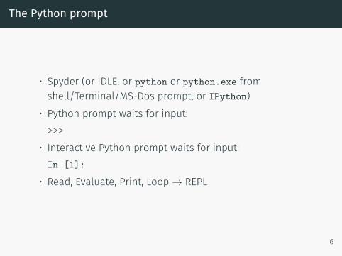
The Python prompt

• Spyder (or IDLE, or python or python.exe fromshell/Terminal/MS-Dos prompt, or IPython)

• Python prompt waits for input:>>>

• Interactive Python prompt waits for input:In [1]:

• Read, Evaluate, Print, Loop→ REPL

6

Hello World program

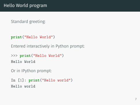
Standard greeting:

print("Hello World")

Entered interactively in Python prompt:

>>> print("Hello World")Hello World

Or in IPython prompt:

In [1]: print("Hello world")Hello world

7

A calculator

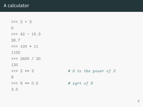
>>> 2 + 35>>> 42 - 15.326.7>>> 100 * 111100>>> 2400 / 20120>>> 2 ** 3 # 2 to the power of 38>>> 9 ** 0.5 # sqrt of 93.0

8

Create variables through assignment

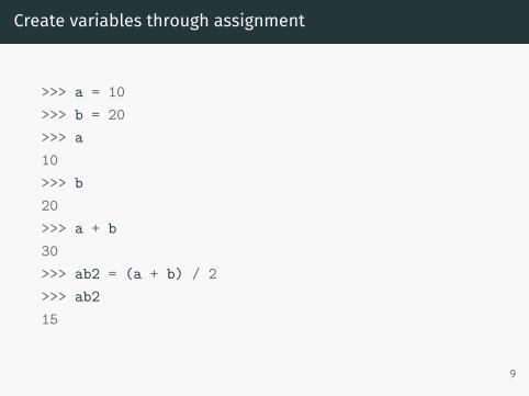
>>> a = 10>>> b = 20>>> a10>>> b20>>> a + b30>>> ab2 = (a + b) / 2>>> ab215

9

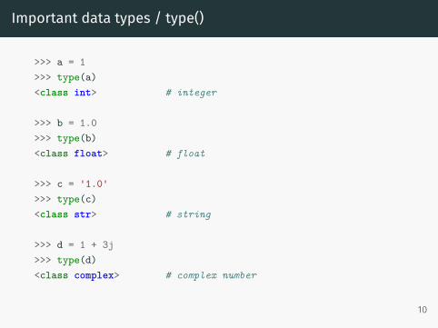
Important data types / type()

>>> a = 1>>> type(a)<class int> # integer

>>> b = 1.0>>> type(b)<class float> # float

>>> c = '1.0'>>> type(c)<class str> # string

>>> d = 1 + 3j>>> type(d)<class complex> # complex number

10

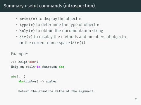
Summary useful commands (introspection)

• print(x) to display the object x• type(x) to determine the type of object x• help(x) to obtain the documentation string• dir(x) to display the methods and members of object x,or the current name space (dir()).

Example:

>>> help("abs")Help on built-in function abs:

abs(...)abs(number) -> number

Return the absolute value of the argument.

11

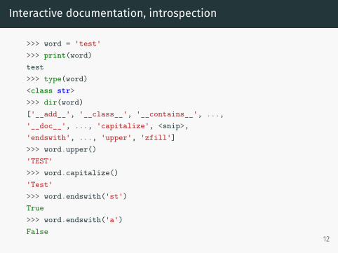
Interactive documentation, introspection

>>> word = 'test'>>> print(word)test>>> type(word)<class str>>>> dir(word)['__add__', '__class__', '__contains__', ...,'__doc__', ..., 'capitalize', <snip>,'endswith', ..., 'upper', 'zfill']>>> word.upper()'TEST'>>> word.capitalize()'Test'>>> word.endswith('st')True>>> word.endswith('a')False

12

Functions

First use of functions

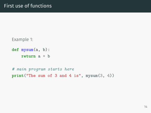
Example 1:

def mysum(a, b):return a + b

# main program starts hereprint("The sum of 3 and 4 is", mysum(3, 4))

14

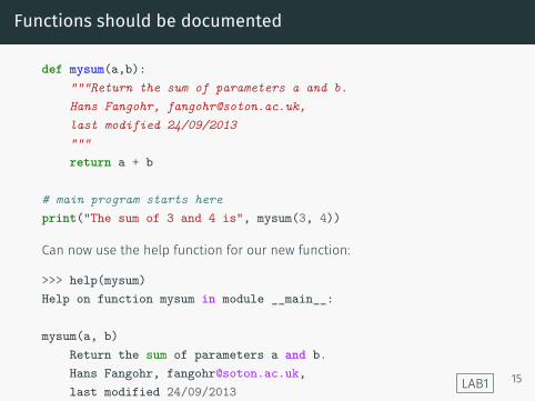
Functions should be documented

def mysum(a,b):"""Return the sum of parameters a and b.Hans Fangohr, fangohr@soton.ac.uk,last modified 24/09/2013"""return a + b

# main program starts hereprint("The sum of 3 and 4 is", mysum(3, 4))

Can now use the help function for our new function:

>>> help(mysum)Help on function mysum in module __main__:

mysum(a, b)Return the sum of parameters a and b.Hans Fangohr, fangohr@soton.ac.uk,last modified 24/09/2013 LAB1 15

Function terminology

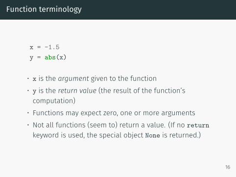
x = -1.5y = abs(x)

• x is the argument given to the function• y is the return value (the result of the function’scomputation)

• Functions may expect zero, one or more arguments• Not all functions (seem to) return a value. (If no returnkeyword is used, the special object None is returned.)

16

Function example

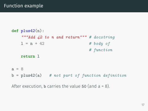
def plus42(n):"""Add 42 to n and return""" # docstringl = n + 42 # body of

# functionreturn l

a = 8b = plus42(a) # not part of function definition

After execution, b carries the value 50 (and a = 8).

17

Summary functions

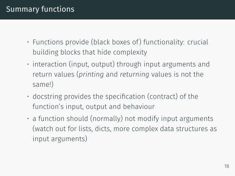
• Functions provide (black boxes of) functionality: crucialbuilding blocks that hide complexity

• interaction (input, output) through input arguments andreturn values (printing and returning values is not thesame!)

• docstring provides the specification (contract) of thefunction’s input, output and behaviour

• a function should (normally) not modify input arguments(watch out for lists, dicts, more complex data structures asinput arguments)

18

Functions printing vs returning values

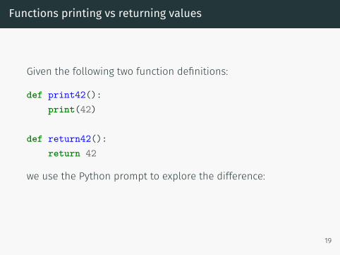
Given the following two function definitions:

def print42():print(42)

def return42():return 42

we use the Python prompt to explore the difference:

19

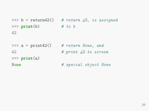
>>> b = return42() # return 42, is assigned>>> print(b) # to b42

>>> a = print42() # return None, and42 # print 42 to screen>>> print(a)None # special object None

20

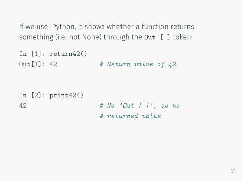
If we use IPython, it shows whether a function returnssomething (i.e. not None) through the Out [ ] token:

In [1]: return42()Out[1]: 42 # Return value of 42

In [2]: print42()42 # No 'Out [ ]', so no

# returned value

21

21

About Python

Python

What is Python?

• High level programming language• interpreted• supports three main programming styles(imperative=procedural, object-oriented, functional)

• General purpose tool, yet good for numeric work withextension libraries

Availability

• Python is free• Python is platform independent (works on Windows,Linux/Unix, Mac OS, …)

23

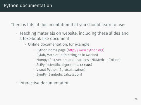
Python documentation

There is lots of documentation that you should learn to use:

• Teaching materials on website, including these slides anda text-book like document

• Online documentation, for example• Python home page (http://www.python.org)• Pylab/Matplotlib (plotting as in Matlab)• Numpy (fast vectors and matrices, (NUMerical PYthon)• SciPy (scientific algorithms, odeint)• Visual Python (3d visualisation)• SymPy (Symbolic calculation)

• interactive documentation

24

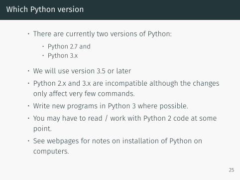
Which Python version

• There are currently two versions of Python:• Python 2.7 and• Python 3.x

• We will use version 3.5 or later• Python 2.x and 3.x are incompatible although the changesonly affect very few commands.

• Write new programs in Python 3 where possible.• You may have to read / work with Python 2 code at somepoint.

• See webpages for notes on installation of Python oncomputers.

25

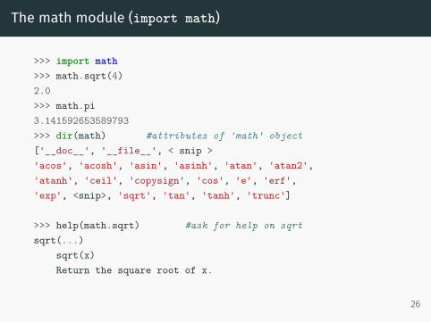
The math module (import math)

>>> import math>>> math.sqrt(4)2.0>>> math.pi3.141592653589793>>> dir(math) #attributes of 'math' object['__doc__', '__file__', < snip >'acos', 'acosh', 'asin', 'asinh', 'atan', 'atan2','atanh', 'ceil', 'copysign', 'cos', 'e', 'erf','exp', <snip>, 'sqrt', 'tan', 'tanh', 'trunc']

>>> help(math.sqrt) #ask for help on sqrtsqrt(...)

sqrt(x)Return the square root of x.

26

Name spaces and modules

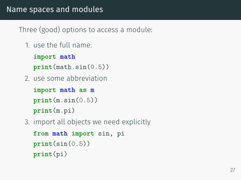
Three (good) options to access a module:

1. use the full name:import mathprint(math.sin(0.5))

2. use some abbreviationimport math as mprint(m.sin(0.5))print(m.pi)

3. import all objects we need explicitlyfrom math import sin, piprint(sin(0.5))print(pi)

27

Python 2: Integer division

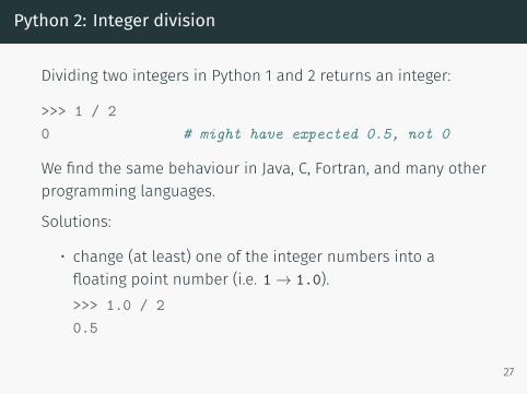
Dividing two integers in Python 1 and 2 returns an integer:

>>> 1 / 20 # might have expected 0.5, not 0

We find the same behaviour in Java, C, Fortran, and many otherprogramming languages.

Solutions:

• change (at least) one of the integer numbers into afloating point number (i.e. 1→ 1.0).>>> 1.0 / 20.5

27

• Or use float function to convert variable to float>>> a = 1>>> b = 2>>> 1 / float(b)0.5

• Or make use of Python’s future division:>>> from __future__ import division>>> 1 / 20.5

If you really want integer division, use // instead of /:

>>> 1 // 20

28

Python 3: Integer division

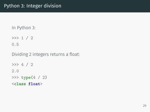
In Python 3:

>>> 1 / 20.5

Dividing 2 integers returns a float:

>>> 4 / 22.0>>> type(4 / 2)<class float>

29

If we want integer division (i.e. an operation that returns aninteger, and/or which replicates the default behaviour ofPython 2), we use //:

>>> 1 // 20

30

Coding style

Coding style

• Python programs must follow Python syntax.• Python programs should follow Python style guide,because

• readability is key (debugging, documentation, team effort)• conventions improve effectiveness

32

Common style guide: PEP8

See http://www.python.org/dev/peps/pep-0008/

• This document gives coding conventions for the Python codecomprising the standard library in the main Python distribution.

• This style guide evolves over time as additional conventions areidentified and past conventions are rendered obsolete by changes inthe language itself.

• Many projects have their own coding style guidelines. In the event ofany conflicts, such project-specific guides take precedence for thatproject.

• One of Guido van Rossum’s key insights is that code is read muchmore often than it is written. The guidelines provided here areintended to improve the readability of code and make it consistentacross the wide spectrum of Python code. ”Readability counts”.

• Sometimes we should not follow the style guide, for example:• When applying the guideline would make the code less readable, even for someone who is used toreading code that follows this PEP.

• To be consistent with surrounding code that also breaks it (maybe for historic reasons) – althoughthis is also an opportunity to clean up someone else’s mess (in true XP style).

33

PEP8 Style guide

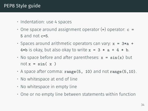
• Indentation: use 4 spaces• One space around assignment operator (=) operator: c =5 and not c=5.

• Spaces around arithmetic operators can vary: x = 3*a +4*b is okay, but also okay to write x = 3 * a + 4 * b.

• No space before and after parentheses: x = sin(x) butnot x = sin( x )

• A space after comma: range(5, 10) and not range(5,10).• No whitespace at end of line• No whitespace in empty line• One or no empty line between statements within function

34

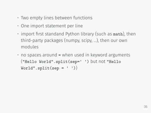
• Two empty lines between functions

• One import statement per line

• import first standand Python library (such as math), thenthird-party packages (numpy, scipy, ...), then our ownmodules

• no spaces around = when used in keyword arguments("Hello World".split(sep=' ') but not "HelloWorld".split(sep = ' '))

35

PEP8 Style Summary

• Try to follow PEP8 guide, in particular for new code• Use tools to help us, for example Spyder editor can showPEP8 violations.Similar tools/plugins are available for Emacs, SublimeText, and other editors.

• pep8 program available to check source code fromcommand line.

36

Conditionals, if-else

Truth values

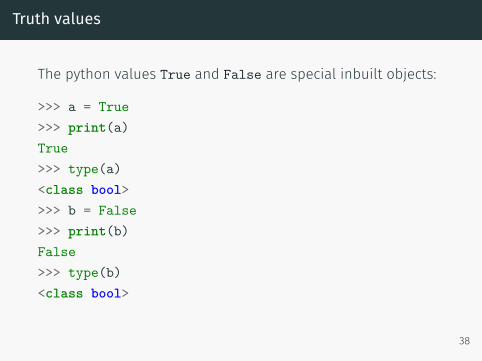
The python values True and False are special inbuilt objects:

>>> a = True>>> print(a)True>>> type(a)<class bool>>>> b = False>>> print(b)False>>> type(b)<class bool>

38

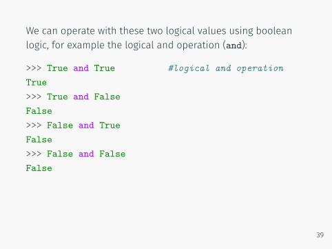
We can operate with these two logical values using booleanlogic, for example the logical and operation (and):

>>> True and True #logical and operationTrue>>> True and FalseFalse>>> False and TrueFalse>>> False and FalseFalse

39

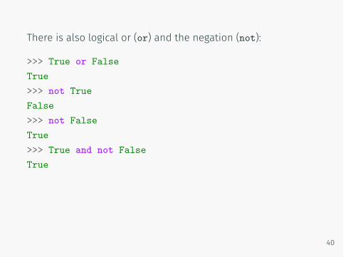
There is also logical or (or) and the negation (not):

>>> True or FalseTrue>>> not TrueFalse>>> not FalseTrue>>> True and not FalseTrue

40

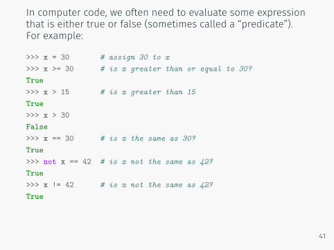
In computer code, we often need to evaluate some expressionthat is either true or false (sometimes called a “predicate”).For example:

>>> x = 30 # assign 30 to x>>> x >= 30 # is x greater than or equal to 30?True>>> x > 15 # is x greater than 15True>>> x > 30False>>> x == 30 # is x the same as 30?True>>> not x == 42 # is x not the same as 42?True>>> x != 42 # is x not the same as 42?True

41

if-then-else

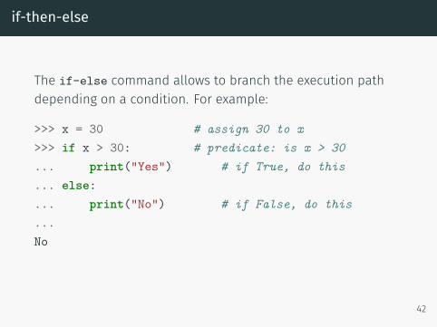
The if-else command allows to branch the execution pathdepending on a condition. For example:

>>> x = 30 # assign 30 to x>>> if x > 30: # predicate: is x > 30... print("Yes") # if True, do this... else:... print("No") # if False, do this...No

42

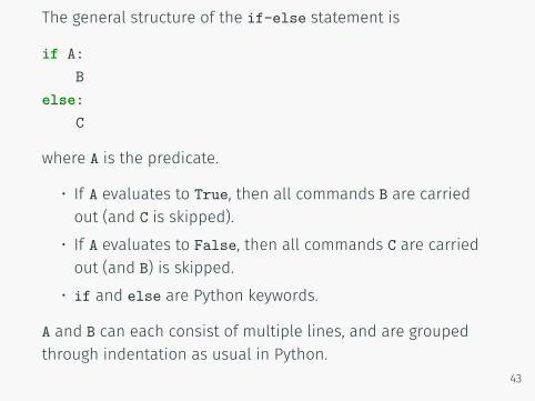
The general structure of the if-else statement is

if A:B

else:C

where A is the predicate.

• If A evaluates to True, then all commands B are carriedout (and C is skipped).

• If A evaluates to False, then all commands C are carriedout (and B) is skipped.

• if and else are Python keywords.

A and B can each consist of multiple lines, and are groupedthrough indentation as usual in Python.

43

if-else example

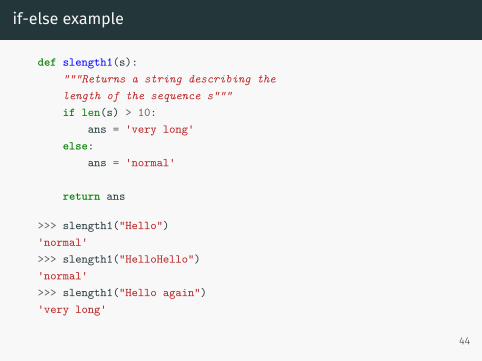
def slength1(s):"""Returns a string describing thelength of the sequence s"""if len(s) > 10:

ans = 'very long'else:

ans = 'normal'

return ans

>>> slength1("Hello")'normal'>>> slength1("HelloHello")'normal'>>> slength1("Hello again")'very long'

44

if-elif-else example

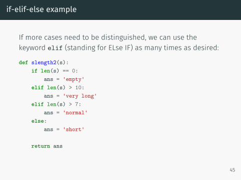
If more cases need to be distinguished, we can use thekeyword elif (standing for ELse IF) as many times as desired:

def slength2(s):if len(s) == 0:

ans = 'empty'elif len(s) > 10:

ans = 'very long'elif len(s) > 7:

ans = 'normal'else:

ans = 'short'

return ans

45

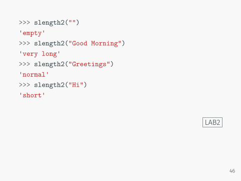
>>> slength2("")'empty'>>> slength2("Good Morning")'very long'>>> slength2("Greetings")'normal'>>> slength2("Hi")'short'

LAB2

46

Sequences

Sequences overview

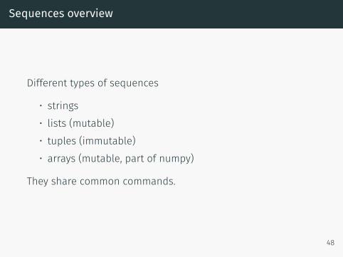
Different types of sequences

• strings• lists (mutable)• tuples (immutable)• arrays (mutable, part of numpy)

They share common commands.

48

Strings

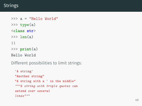
>>> a = "Hello World">>> type(a)<class str>>>> len(a)11>>> print(a)Hello World

Different possibilities to limit strings:

'A string'"Another string""A string with a ' in the middle""""A string with triple quotes canextend over severallines"""

49

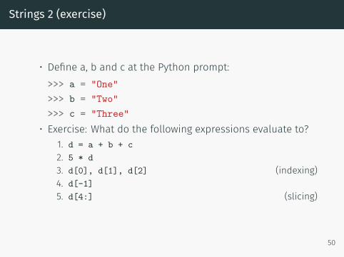
Strings 2 (exercise)

• Define a, b and c at the Python prompt:>>> a = "One">>> b = "Two">>> c = "Three"

• Exercise: What do the following expressions evaluate to?1. d = a + b + c2. 5 * d3. d[0], d[1], d[2] (indexing)4. d[-1]5. d[4:] (slicing)

50

Strings 3 (exercise)

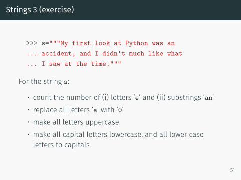
>>> s="""My first look at Python was an... accident, and I didn't much like what... I saw at the time."""

For the string s:

• count the number of (i) letters ’e’ and (ii) substrings ’an’• replace all letters ’a’ with ’0’• make all letters uppercase• make all capital letters lowercase, and all lower caseletters to capitals

51

Lists

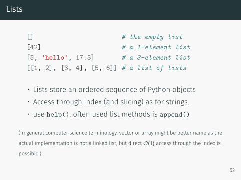
[] # the empty list[42] # a 1-element list[5, 'hello', 17.3] # a 3-element list[[1, 2], [3, 4], [5, 6]] # a list of lists

• Lists store an ordered sequence of Python objects• Access through index (and slicing) as for strings.• use help(), often used list methods is append()

(In general computer science terminology, vector or array might be better name as the

actual implementation is not a linked list, but direct O(1) access through the index is

possible.)

52

Example program: using lists

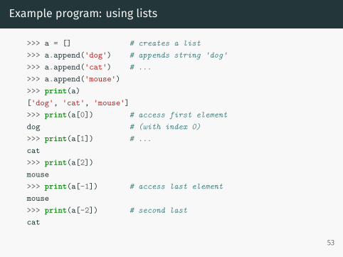
>>> a = [] # creates a list>>> a.append('dog') # appends string 'dog'>>> a.append('cat') # ...>>> a.append('mouse')>>> print(a)['dog', 'cat', 'mouse']>>> print(a[0]) # access first elementdog # (with index 0)>>> print(a[1]) # ...cat>>> print(a[2])mouse>>> print(a[-1]) # access last elementmouse>>> print(a[-2]) # second lastcat

53

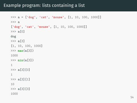
Example program: lists containing a list

>>> a = ['dog', 'cat', 'mouse', [1, 10, 100, 1000]]>>> a['dog', 'cat', 'mouse', [1, 10, 100, 1000]]>>> a[0]dog>>> a[3][1, 10, 100, 1000]>>> max(a[3])1000>>> min(a[3])1>>> a[3][0]1>>> a[3][1]10>>> a[3][3]1000

54

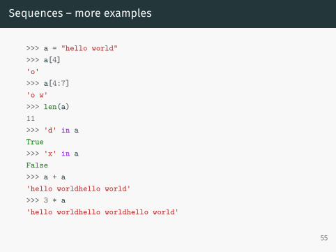
Sequences – more examples

>>> a = "hello world">>> a[4]'o'>>> a[4:7]'o w'>>> len(a)11>>> 'd' in aTrue>>> 'x' in aFalse>>> a + a'hello worldhello world'>>> 3 * a'hello worldhello worldhello world'

55

Tuples

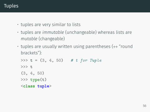
• tuples are very similar to lists• tuples are immutable (unchangeable) whereas lists aremutable (changeable)

• tuples are usually written using parentheses (↔ “roundbrackets”):>>> t = (3, 4, 50) # t for Tuple>>> t(3, 4, 50)>>> type(t)<class tuple>

56

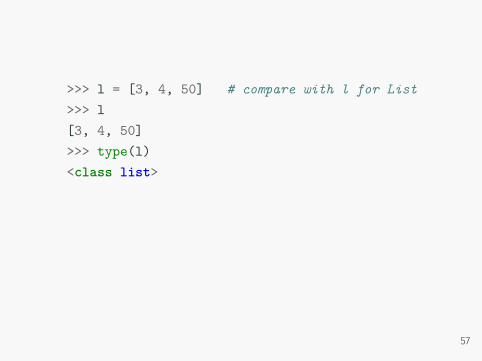
>>> l = [3, 4, 50] # compare with l for List>>> l[3, 4, 50]>>> type(l)<class list>

57

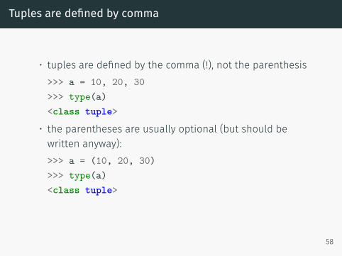
Tuples are defined by comma

• tuples are defined by the comma (!), not the parenthesis>>> a = 10, 20, 30>>> type(a)<class tuple>

• the parentheses are usually optional (but should bewritten anyway):>>> a = (10, 20, 30)>>> type(a)<class tuple>

58

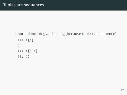
Tuples are sequences

• normal indexing and slicing (because tuple is a sequence)>>> t[1]4>>> t[:-1](3, 4)

59

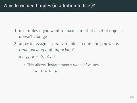
Why do we need tuples (in addition to lists)?

1. use tuples if you want to make sure that a set of objectsdoesn’t change.

2. allow to assign several variables in one line (known astuple packing and unpacking)x, y, z = 0, 0, 1

• This allows ’ instantaneous swap’ of values:a, b = b, a

60

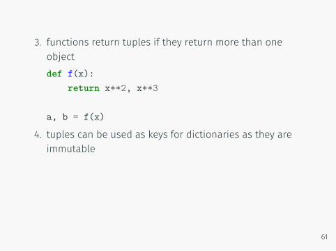
3. functions return tuples if they return more than oneobjectdef f(x):

return x**2, x**3

a, b = f(x)

4. tuples can be used as keys for dictionaries as they areimmutable

61

(Im)mutables

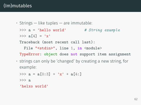
• Strings — like tuples — are immutable:>>> a = 'hello world' # String example>>> a[4] = 'x'Traceback (most recent call last):

File "<stdin>", line 1, in <module>TypeError: object does not support item assignment

• strings can only be ’changed’ by creating a new string, forexample:>>> a = a[0:3] + 'x' + a[4:]>>> a'helxo world'

62

Summary sequences

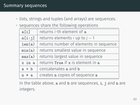
• lists, strings and tuples (and arrays) are sequences.• sequences share the following operations

a[i] returns i-th element of aa[i:j] returns elements i up to j− 1len(a) returns number of elements in sequencemin(a) returns smallest value in sequencemax(a) returns largest value in sequencex in a returns True if x is element in aa + b concatenates a and bn * a creates n copies of sequence a

In the table above, a and b are sequences, i, j and n areintegers.

63

Conversions

• We can convert any sequence into a tuple using the tuplefunction:>>> tuple([1, 4, "dog"])(1, 4, 'dog')

• Similarly, the list function, converts sequences into lists:>>> list((10, 20, 30))[10, 20, 30]

• Looking ahead to iterators, we note that list and tuple canalso convert from iterators:>>> list(range(5))[0, 1, 2, 3, 4]And if you ever need to create an iterator from a sequence, theiter function can this:>>> iter([1, 2, 3])<list_iterator object at 0x1013f1fd0> 64

Loops

Introduction loops

Computers are good at repeating tasks (often the same taskfor many different sets of data).

Loops are the way to execute the same (or very similar) tasksrepeatedly (“ in a loop”).

Python provides the “for loop” and the “while loop”.

66

Example program: for-loop

animals = ['dog', 'cat', 'mouse']

for animal in animals:print("This is the {}".format(animal))

produces

This is the dogThis is the catThis is the mouse

The for-loop iterates through the sequence animals andassigns the values in the sequence subsequently to the nameanimal.

67

Iterating over integers

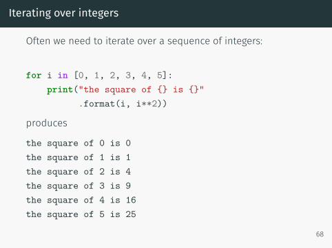
Often we need to iterate over a sequence of integers:

for i in [0, 1, 2, 3, 4, 5]:print("the square of {} is {}"

.format(i, i**2))

produces

the square of 0 is 0the square of 1 is 1the square of 2 is 4the square of 3 is 9the square of 4 is 16the square of 5 is 25

68

Iterating over integers with the range iterator

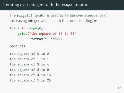
The range(n) iterator is used to iterate over a sequence ofincreasing integer values up to (but not including) n:

for i in range(6):print("the square of {} is {}"

.format(i, i**2))

produces

the square of 0 is 0the square of 1 is 1the square of 2 is 4the square of 3 is 9the square of 4 is 16the square of 5 is 25

69

The range iterator

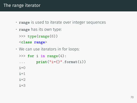
• range is used to iterate over integer sequences• range has its own type:>>> type(range(6))<class range>

• We can use iterators in for loops:>>> for i in range(4):... print("i={}".format(i))i=0i=1i=2i=3

70

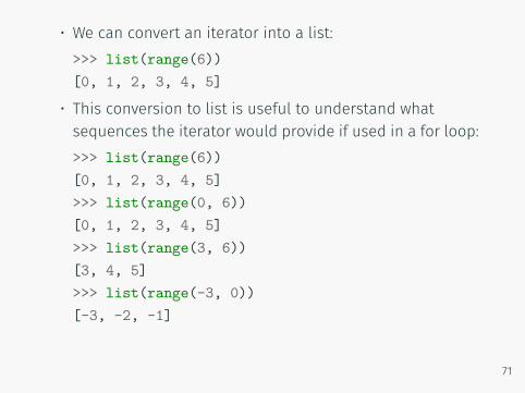
• We can convert an iterator into a list:>>> list(range(6))[0, 1, 2, 3, 4, 5]

• This conversion to list is useful to understand whatsequences the iterator would provide if used in a for loop:>>> list(range(6))[0, 1, 2, 3, 4, 5]>>> list(range(0, 6))[0, 1, 2, 3, 4, 5]>>> list(range(3, 6))[3, 4, 5]>>> list(range(-3, 0))[-3, -2, -1]

71

The range iteratorrange([start,] stop [,step]) iterates over integers fromstart to but not including stop, in steps of step.

start defaults to 0 and step defaults to 1.

Examples:

>>> list(range(0, 10))[0, 1, 2, 3, 4, 5, 6, 7, 8, 9]>>> list(range(0, 10, 2))[0, 2, 4, 6, 8]>>> list(range(5, 4))[] # no iterations

(Note that range objects are sequences.)

72

Iterating over sequences with for-loop

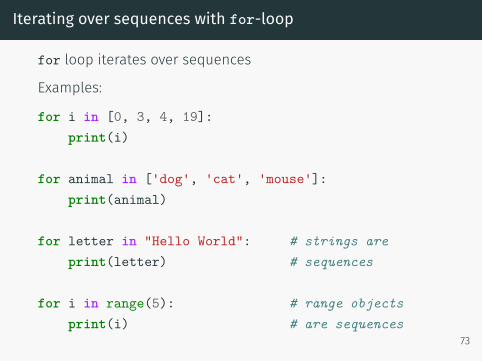
for loop iterates over sequences

Examples:

for i in [0, 3, 4, 19]:print(i)

for animal in ['dog', 'cat', 'mouse']:print(animal)

for letter in "Hello World": # strings areprint(letter) # sequences

for i in range(5): # range objectsprint(i) # are sequences

73

Reminder: If-then-else

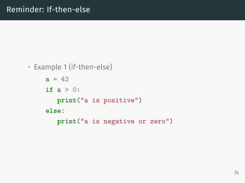
• Example 1 (if-then-else)a = 42if a > 0:

print("a is positive")else:

print("a is negative or zero")

74

Another iteration example

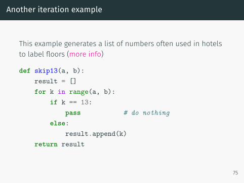
This example generates a list of numbers often used in hotelsto label floors (more info)

def skip13(a, b):result = []for k in range(a, b):

if k == 13:pass # do nothing

else:result.append(k)

return result

75

Exercise range_double

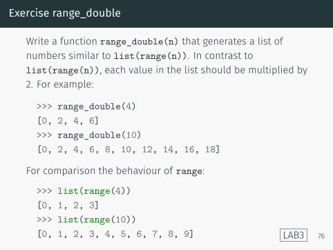
Write a function range_double(n) that generates a list ofnumbers similar to list(range(n)). In contrast tolist(range(n)), each value in the list should be multiplied by2. For example:

>>> range_double(4)[0, 2, 4, 6]>>> range_double(10)[0, 2, 4, 6, 8, 10, 12, 14, 16, 18]

For comparison the behaviour of range:

>>> list(range(4))[0, 1, 2, 3]>>> list(range(10))[0, 1, 2, 3, 4, 5, 6, 7, 8, 9] LAB3 76

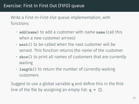
Exercise: First In First Out (FIFO) queue

Write a First-In-First-Out queue implementation, withfunctions:

• add(name) to add a customer with name name (call thiswhen a new customer arrives)

• next() to be called when the next customer will beserved. This function returns the name of the customer

• show() to print all names of customers that are currentlywaiting

• length() to return the number of currently waitingcustomers

Suggest to use a global variable q and define this in the firstline of the file by assigning an empty list: q = [].

77

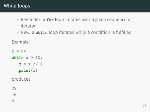
While loops

• Reminder: a for loop iterates over a given sequence oriterator

• New: a while loop iterates while a condition is fulfilled

Example:

x = 64while x > 10:

x = x // 2print(x)

produces

32168

78

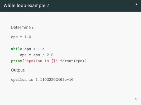
While loop example 2 *

Determine ϵ:

eps = 1.0

while eps + 1 > 1:eps = eps / 2.0

print("epsilon is {}".format(eps))

Output:

epsilon is 1.11022302463e-16

79

79

Some things revisited

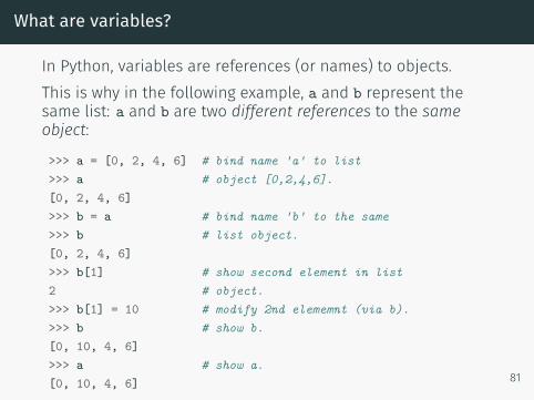
What are variables?

In Python, variables are references (or names) to objects.This is why in the following example, a and b represent thesame list: a and b are two different references to the sameobject:

>>> a = [0, 2, 4, 6] # bind name 'a' to list>>> a # object [0,2,4,6].[0, 2, 4, 6]>>> b = a # bind name 'b' to the same>>> b # list object.[0, 2, 4, 6]>>> b[1] # show second element in list2 # object.>>> b[1] = 10 # modify 2nd elememnt (via b).>>> b # show b.[0, 10, 4, 6]>>> a # show a.[0, 10, 4, 6] 81

id, == and is

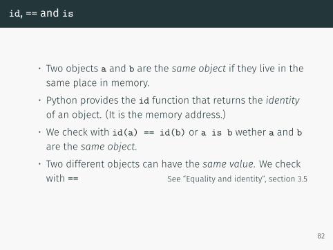
• Two objects a and b are the same object if they live in thesame place in memory.

• Python provides the id function that returns the identityof an object. (It is the memory address.)

• We check with id(a) == id(b) or a is b wether a and bare the same object.

• Two different objects can have the same value. We checkwith == See “Equality and identity“, section 3.5

82

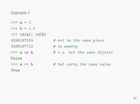
Example 1

>>> a = 1>>> b = 1.0>>> id(a); id(b)4298187624 # not in the same place4298197712 # in memory>>> a is b # i.e. not the same objectsFalse>>> a == b # but carry the same valueTrue

83

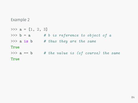
Example 2

>>> a = [1, 2, 3]>>> b = a # b is reference to object of a>>> a is b # thus they are the sameTrue>>> a == b # the value is (of course) the sameTrue

84

Functions – side effect

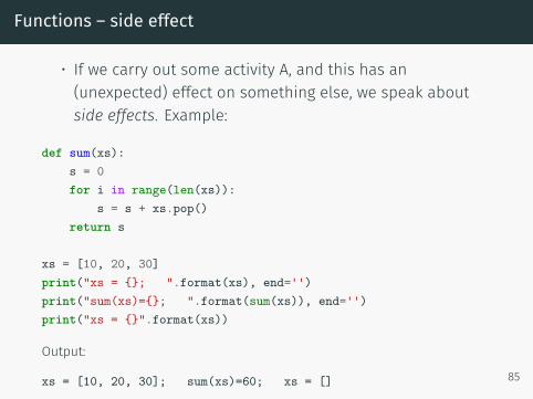
• If we carry out some activity A, and this has an(unexpected) effect on something else, we speak aboutside effects. Example:

def sum(xs):s = 0for i in range(len(xs)):

s = s + xs.pop()return s

xs = [10, 20, 30]print("xs = {}; ".format(xs), end='')print("sum(xs)={}; ".format(sum(xs)), end='')print("xs = {}".format(xs))

Output:

xs = [10, 20, 30]; sum(xs)=60; xs = [] 85

Functions - side effect 2

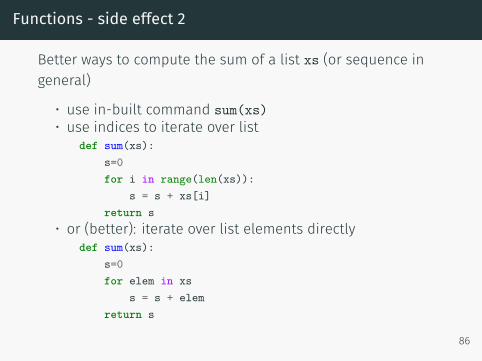
Better ways to compute the sum of a list xs (or sequence ingeneral)

• use in-built command sum(xs)• use indices to iterate over list

def sum(xs):s=0for i in range(len(xs)):

s = s + xs[i]return s

• or (better): iterate over list elements directlydef sum(xs):

s=0for elem in xs

s = s + elemreturn s

86

To print or to return?

• A function that returns the control flow through thereturn keyword, will return the object given after return.

• A function that does not use the return keyword, returnsthe special object None.

• Generally, functions should return a value• Generally, functions should not print anything• Calling functions from the prompt can cause someconfusion here: if the function returns a value and thevalue is not assigned, it will be printed.

• See slide 19.

87

Reading and Writing files

File input/output

It is a (surprisingly) common task to

• read some input data file• do some calculation/filtering/processing with the data• write some output data file with results

Python distinguishes between

• text files ('t')• binary files 'b')

If we don’t specify the file type, Python assumes we mean textfiles.

89

Writing a text file

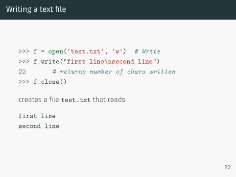
>>> f = open('test.txt', 'w') # Write>>> f.write("first line\nsecond line")22 # returns number of chars written>>> f.close()

creates a file test.txt that reads

first linesecond line

90

• To write data, we need to open the file with 'w' mode:f = open('test.txt', 'w')

By default, Python assumes we mean text files. However,we can be explicit and say that we want to create a Textfile for Writing:

f = open('test.txt', 'tw')

• If the file exists, it will be overridden with an empty filewhen the open command is executed.

• The file object f has a method f.write which takes astring as in input argument.

• Must close file at the end of writing process usingf.close().

91

Reading a text file

We create a file object f using

>>> f = open('test.txt', 'r') # Read

and have different ways of reading the data:

1. f.readlines() returns a list of strings (each being oneline)

>>> f = open('test.txt', 'r')>>> lines = f.readlines()>>> f.close()>>> lines['first line\n', 'second line']

92

2. f.read() returns one long string for the whole file>>> f = open('test.txt', 'r')>>> data = f.read()>>> f.close()>>> data'first line\nsecond line'

3. Use text file f as an iterable object: process one line ineach iteration (important for large files):>>> f = open('test.txt', 'r')>>> for line in f:... print(line, end='')...first linesecond line>>> f.close()

93

Opening and automatic file closing through context manager

Python provides context managers that we use using with. Forthe file access:

>>> with open('test.txt', 'r') as f:... data = f.read()...>>> data'first line\nsecond line'

If we use the file context manager, it will close the fileautomatically (when the control flows leaves the indentedblock).

Once you are familiar with file access, we recommend you usethis method.

94

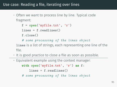
Use case: Reading a file, iterating over lines

• Often we want to process line by line. Typical codefragment:

f = open('myfile.txt', 'r')lines = f.readlines()f.close()# some processing of the lines object

lines is a list of strings, each representing one line of thefile.

• It is good practice to close a file as soon as possible.• Equivalent example using the context manager:

with open('myfile.txt', 'r') as f:lines = f.readlines()

# some processing of the lines object

95

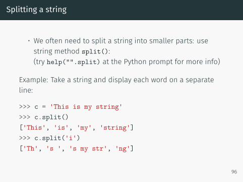
Splitting a string

• We often need to split a string into smaller parts: usestring method split():(try help("".split) at the Python prompt for more info)

Example: Take a string and display each word on a separateline:

>>> c = 'This is my string'>>> c.split()['This', 'is', 'my', 'string']>>> c.split('i')['Th', 's ', 's my str', 'ng']

96

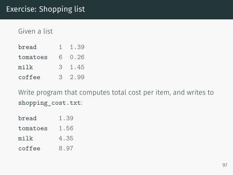
Exercise: Shopping list

Given a list

bread 1 1.39tomatoes 6 0.26milk 3 1.45coffee 3 2.99

Write program that computes total cost per item, and writes toshopping_cost.txt:

bread 1.39tomatoes 1.56milk 4.35coffee 8.97

97

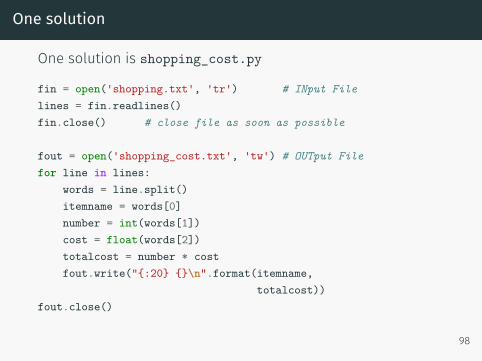
One solution

One solution is shopping_cost.py

fin = open('shopping.txt', 'tr') # INput Filelines = fin.readlines()fin.close() # close file as soon as possible

fout = open('shopping_cost.txt', 'tw') # OUTput Filefor line in lines:

words = line.split()itemname = words[0]number = int(words[1])cost = float(words[2])totalcost = number * costfout.write("{:20} {}\n".format(itemname,

totalcost))fout.close()

98

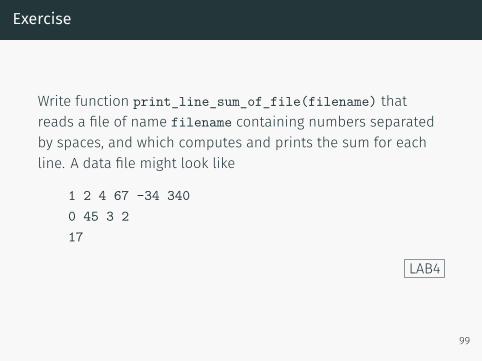
Exercise

Write function print_line_sum_of_file(filename) thatreads a file of name filename containing numbers separatedby spaces, and which computes and prints the sum for eachline. A data file might look like

1 2 4 67 -34 3400 45 3 217

LAB4

99

Binary files

• Files that store binary data are opened using the 'b' flag(instead of 't' for Text):

f = open('data.dat', 'br')

• For text files, we read and write str objects. For binaryfiles, use the bytes type instead.

• By default, store data in text files. Text files are humanreadable (that’s good) but take more disk space thanbinary files.

• Reading and writing binary data is outside the scope ofthis introductory module. If you need it, do learn aboutthe struct module.

100

100

Exceptions

Exceptions

• Errors arising during the execution of a program result in“exceptions” being ’raised’ (or ’thrown’).

• We have seen exceptions before, for example whendividing by zero:>>> 4.5 / 0Traceback (most recent call last):

File "<stdin>", line 1, in <module>ZeroDivisionError: float division by zeroor when we try to access an undefined variable:

102

>>> print(x)Traceback (most recent call last):

File "<stdin>", line 1, in <module>NameError: name 'x' is not defined

• Exceptions are a modern way of dealing with errorsituations

• We will now see how• what exceptions are coming with Python• we can “catch” exceptions• we can raise (“throw”) exceptions in our code

103

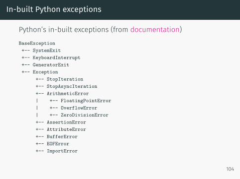
In-built Python exceptions

Python’s in-built exceptions (from documentation)

BaseException+-- SystemExit+-- KeyboardInterrupt+-- GeneratorExit+-- Exception

+-- StopIteration+-- StopAsyncIteration+-- ArithmeticError| +-- FloatingPointError| +-- OverflowError| +-- ZeroDivisionError+-- AssertionError+-- AttributeError+-- BufferError+-- EOFError+-- ImportError

104

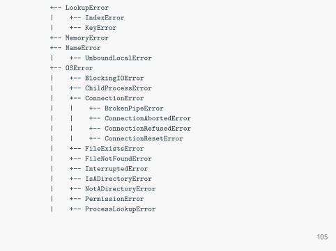
+-- LookupError| +-- IndexError| +-- KeyError+-- MemoryError+-- NameError| +-- UnboundLocalError+-- OSError| +-- BlockingIOError| +-- ChildProcessError| +-- ConnectionError| | +-- BrokenPipeError| | +-- ConnectionAbortedError| | +-- ConnectionRefusedError| | +-- ConnectionResetError| +-- FileExistsError| +-- FileNotFoundError| +-- InterruptedError| +-- IsADirectoryError| +-- NotADirectoryError| +-- PermissionError| +-- ProcessLookupError

105

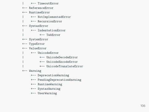
| +-- TimeoutError+-- ReferenceError+-- RuntimeError| +-- NotImplementedError| +-- RecursionError+-- SyntaxError| +-- IndentationError| +-- TabError+-- SystemError+-- TypeError+-- ValueError| +-- UnicodeError| +-- UnicodeDecodeError| +-- UnicodeEncodeError| +-- UnicodeTranslateError+-- Warning

+-- DeprecationWarning+-- PendingDeprecationWarning+-- RuntimeWarning+-- SyntaxWarning+-- UserWarning

106

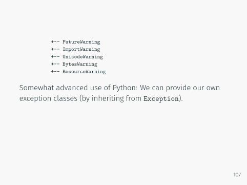
+-- FutureWarning+-- ImportWarning+-- UnicodeWarning+-- BytesWarning+-- ResourceWarning

Somewhat advanced use of Python: We can provide our ownexception classes (by inheriting from Exception).

107

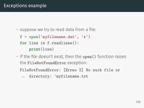
Exceptions example

• suppose we try to read data from a file:f = open('myfilename.dat', 'r')for line in f.readlines():

print(line)

• If the file doesn’t exist, then the open() function raisesthe FileNotFoundError exception:FileNotFoundError: [Errno 2] No such file or

directory: 'myfilename.txt↪→

108

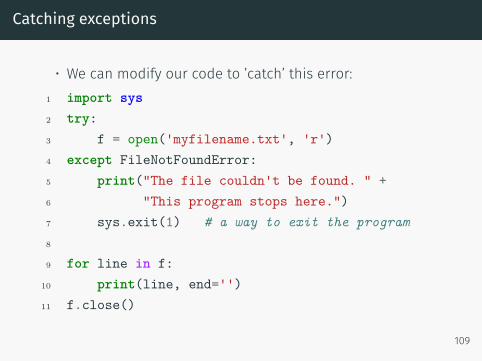
Catching exceptions

• We can modify our code to ’catch’ this error:1 import sys2 try:3 f = open('myfilename.txt', 'r')4 except FileNotFoundError:5 print("The file couldn't be found. " +6 "This program stops here.")7 sys.exit(1) # a way to exit the program8

9 for line in f:10 print(line, end='')11 f.close()

109

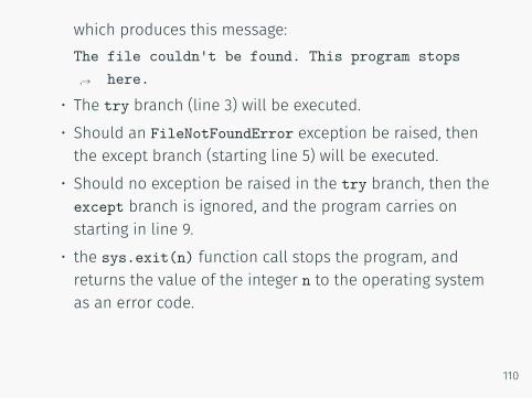
which produces this message:The file couldn't be found. This program stops

here.↪→

• The try branch (line 3) will be executed.• Should an FileNotFoundError exception be raised, thenthe except branch (starting line 5) will be executed.

• Should no exception be raised in the try branch, then theexcept branch is ignored, and the program carries onstarting in line 9.

• the sys.exit(n) function call stops the program, andreturns the value of the integer n to the operating systemas an error code.

110

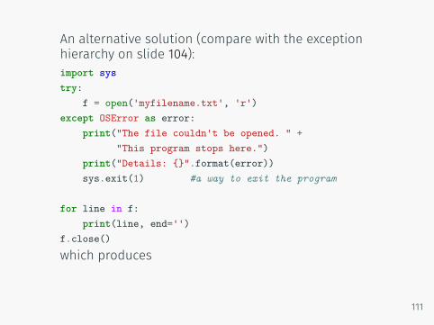
An alternative solution (compare with the exceptionhierarchy on slide 104):import systry:

f = open('myfilename.txt', 'r')except OSError as error:

print("The file couldn't be opened. " +"This program stops here.")

print("Details: {}".format(error))sys.exit(1) #a way to exit the program

for line in f:print(line, end='')

f.close()which produces

111

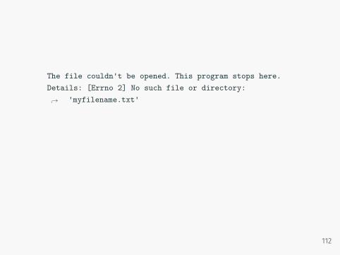
The file couldn't be opened. This program stops here.Details: [Errno 2] No such file or directory:

'myfilename.txt'↪→

112

Catching exceptions summary

• Catching exceptions allows us to take action on errors thatoccur

• For the file-reading example, we could ask the user toprovide another file name if the file can’t be opened.

• Catching an exception once an error has occurred may beeasier than checking beforehand whether a problem willoccur (“It is easier to ask forgiveness than getpermission”.)

113

Raising exceptions

• Because exceptions are Python’s way of dealing withruntime errors, we should use exceptions to report errorsthat occur in our own code.

• To raise a ValueError exception, we useraise ValueError("Message")and can attach a message "Message" (of type string) tothat exception which can be seen when the exception isreported or caught.

114

Raising exceptions example

>>> raise ValueError("Some problem occurred")Traceback (most recent call last):File "<stdin>", line 1, in <module>

ValueError: Some problem occurred

115

Raising NotImplementedError Example

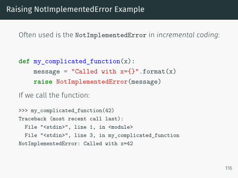
Often used is the NotImplementedError in incremental coding:

def my_complicated_function(x):message = "Called with x={}".format(x)raise NotImplementedError(message)

If we call the function:

>>> my_complicated_function(42)Traceback (most recent call last):File "<stdin>", line 1, in <module>File "<stdin>", line 3, in my_complicated_function

NotImplementedError: Called with x=42

116

Exercise

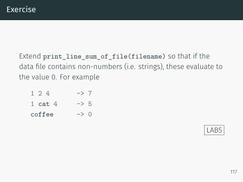
Extend print_line_sum_of_file(filename) so that if thedata file contains non-numbers (i.e. strings), these evaluate tothe value 0. For example

1 2 4 -> 71 cat 4 -> 5coffee -> 0

LAB5

117

117

Printing

Printing basics

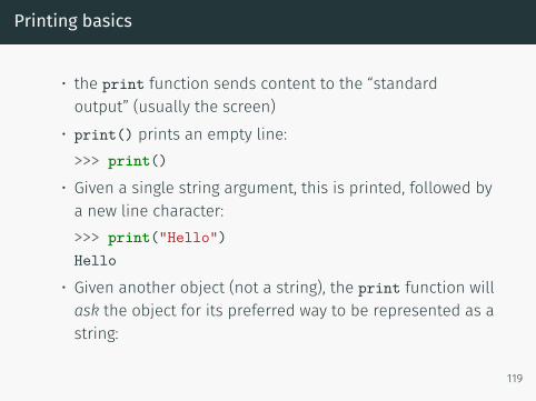
• the print function sends content to the “standardoutput” (usually the screen)

• print() prints an empty line:>>> print()

• Given a single string argument, this is printed, followed bya new line character:>>> print("Hello")Hello

• Given another object (not a string), the print function willask the object for its preferred way to be represented as astring:

119

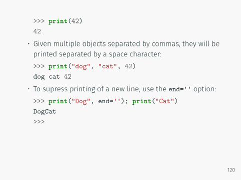
>>> print(42)42

• Given multiple objects separated by commas, they will beprinted separated by a space character:>>> print("dog", "cat", 42)dog cat 42

• To supress printing of a new line, use the end='' option:>>> print("Dog", end=''); print("Cat")DogCat>>>

120

Common strategy for the print command

• Construct some string s, then print this string using theprint function>>> s = "I am the string to be printed">>> print(s)I am the string to be printed

• The question is, how can we construct the string s? Wetalk about string formatting.

121

String formatting: the percentage (%) operator

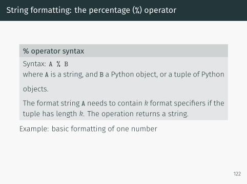
% operator syntaxSyntax: A % Bwhere A is a string, and B a Python object, or a tuple of Python

objects.

The format string A needs to contain k format specifiers if thetuple has length k. The operation returns a string.

Example: basic formatting of one number

122

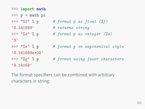
>>> import math>>> p = math.pi>>> "%f" % p # format p as float (%f)'3.141593' # returns string>>> "%d" % p # format p as integer (%d)'3'>>> "%e" % p # format p in exponential style'3.141593e+00'>>> "%g" % p # format using fewer characters'3.14159'

The format specifiers can be combined with arbitrarycharacters in string:

123

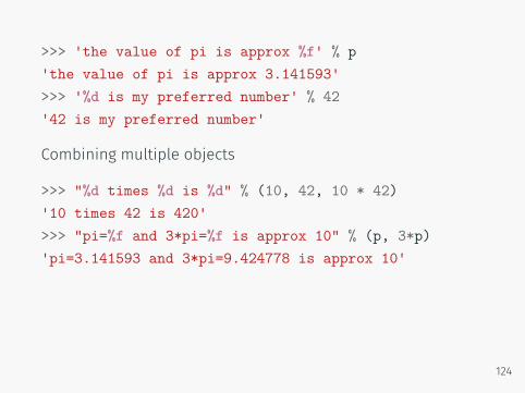
>>> 'the value of pi is approx %f' % p'the value of pi is approx 3.141593'>>> '%d is my preferred number' % 42'42 is my preferred number'

Combining multiple objects

>>> "%d times %d is %d" % (10, 42, 10 * 42)'10 times 42 is 420'>>> "pi=%f and 3*pi=%f is approx 10" % (p, 3*p)'pi=3.141593 and 3*pi=9.424778 is approx 10'

124

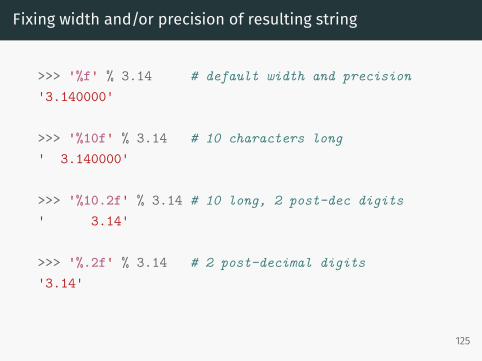
Fixing width and/or precision of resulting string

>>> '%f' % 3.14 # default width and precision'3.140000'

>>> '%10f' % 3.14 # 10 characters long' 3.140000'

>>> '%10.2f' % 3.14 # 10 long, 2 post-dec digits' 3.14'

>>> '%.2f' % 3.14 # 2 post-decimal digits'3.14'

125

>>> '%.14f' % 3.14 # 14 post-decimal digits'3.14000000000000'

There is also the format specifier %s that expects a string, oran object that can provide its own string representation.

Combined with a width specifier, this can be used to aligncolumns of strings in tables:

>>> "%10s" % "apple"' apple'>>> "%10s" % "banana"' banana'

126

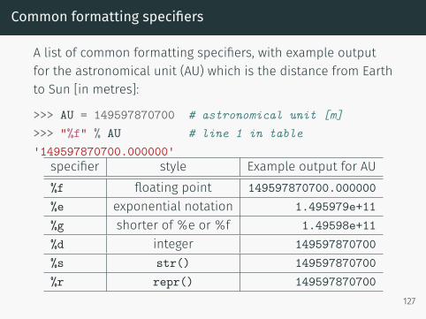
Common formatting specifiers

A list of common formatting specifiers, with example outputfor the astronomical unit (AU) which is the distance from Earthto Sun [in metres]:

>>> AU = 149597870700 # astronomical unit [m]>>> "%f" % AU # line 1 in table'149597870700.000000'

specifier style Example output for AU%f floating point 149597870700.000000%e exponential notation 1.495979e+11%g shorter of %e or %f 1.49598e+11%d integer 149597870700%s str() 149597870700%r repr() 149597870700

127

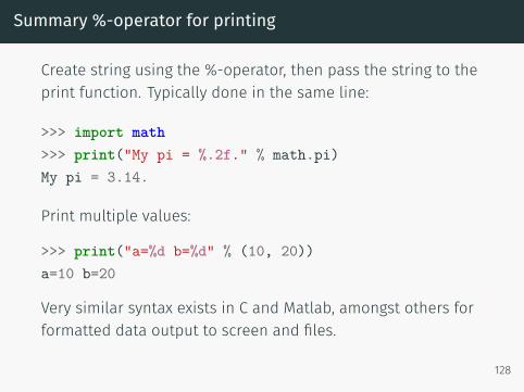
Summary %-operator for printing

Create string using the %-operator, then pass the string to theprint function. Typically done in the same line:

>>> import math>>> print("My pi = %.2f." % math.pi)My pi = 3.14.

Print multiple values:

>>> print("a=%d b=%d" % (10, 20))a=10 b=20

Very similar syntax exists in C and Matlab, amongst others forformatted data output to screen and files.

128

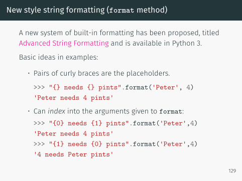
New style string formatting (format method)

A new system of built-in formatting has been proposed, titledAdvanced String Formatting and is available in Python 3.

Basic ideas in examples:

• Pairs of curly braces are the placeholders.

>>> "{} needs {} pints".format('Peter', 4)'Peter needs 4 pints'

• Can index into the arguments given to format:>>> "{0} needs {1} pints".format('Peter',4)'Peter needs 4 pints'>>> "{1} needs {0} pints".format('Peter',4)'4 needs Peter pints'

129

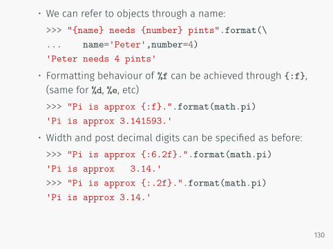
• We can refer to objects through a name:>>> "{name} needs {number} pints".format(\... name='Peter',number=4)'Peter needs 4 pints'

• Formatting behaviour of %f can be achieved through {:f},(same for %d, %e, etc)>>> "Pi is approx {:f}.".format(math.pi)'Pi is approx 3.141593.'

• Width and post decimal digits can be specified as before:>>> "Pi is approx {:6.2f}.".format(math.pi)'Pi is approx 3.14.'>>> "Pi is approx {:.2f}.".format(math.pi)'Pi is approx 3.14.'

130

This is a powerful and elegant way of string formatting.

Further Reading

• Exampleshttp://docs.python.org/library/string.html#format-examples

• Python Enhancement Proposal 3101

131

What formatting should I use?

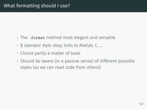
• The .format method most elegant and versatile

• % operator style okay, links to Matlab, C, ...

• Choice partly a matter of taste

• Should be aware (in a passive sense) of different possiblestyles (so we can read code from others)

132

Changes from Python 2 to Python 3: print

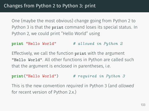
One (maybe the most obvious) change going from Python 2 toPython 3 is that the print command loses its special status. InPython 2, we could print ”Hello World” using

print "Hello World" # allowed in Python 2

Effectively, we call the function print with the argument"Hello World". All other functions in Python are called suchthat the argument is enclosed in parentheses, i.e.

print("Hello World") # required in Python 3

This is the new convention required in Python 3 (and allowedfor recent version of Python 2.x.)

133

The str function and __str__ method

All objects in Python should provide a method __str__ whichreturns a nice string representation of the object.

This method a.__str__ is called when we apply the strfunction to object a:

>>> a = 3.14>>> a.__str__()'3.14'>>> str(a)'3.14'

134

The str function is extremely convenient as it allows us toprint more complicated objects, such as a list

>>> b = [3, 4.2, ['apple', 'banana'], (0, 1)]>>> str(b)"[3, 4.2, ['apple', 'banana'], (0, 1)]"

The string method x.__str__ of object x is called implicitly,when we

• use the ”%s” format specifier in %-operator formatting toprint x

• use the ”{}” format specifier in .format to print x• pass the object x directly to the print command

135

>>> b = [3, 4.2, ['apple', 'banana'], (0, 1)]>>> b.__str__()"[3, 4.2, ['apple', 'banana'], (0, 1)]">>> str(b)"[3, 4.2, ['apple', 'banana'], (0, 1)]">>> "%s" % b"[3, 4.2, ['apple', 'banana'], (0, 1)]">>> "{}".format(b)"[3, 4.2, ['apple', 'banana'], (0, 1)]">>> print(b)[3, 4.2, ['apple', 'banana'], (0, 1)]

136

The repr function and __repr__ method

• The repr function should convert a given object into an asaccurate as possible string representation

• The str function, in contrast, aims to return an “informal”representation of the object that is useful to humans.

• The repr function will generally provide a more detailedstring than str.

• Applying repr to the object x will attempt to callx.__repr__().

137

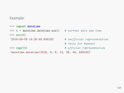
Example:

>>> import datetime>>> t = datetime.datetime.now() # current date and time>>> str(t)'2016-09-08 14:28:48.648192' # inofficial representation

# (nice for humans)>>> repr(t) # official representation'datetime.datetime(2016, 9, 8, 14, 28, 48, 648192)'

138

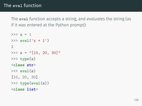
The eval function

The eval function accepts a string, and evaluates the string (asif it was entered at the Python prompt):

>>> x = 1>>> eval('x + 1')2>>> s = "[10, 20, 30]">>> type(s)<class str>>>> eval(s)[10, 20, 30]>>> type(eval(s))<class list>

139

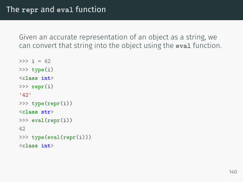
The repr and eval function

Given an accurate representation of an object as a string, wecan convert that string into the object using the eval function.

>>> i = 42>>> type(i)<class int>>>> repr(i)'42'>>> type(repr(i))<class str>>>> eval(repr(i))42>>> type(eval(repr(i)))<class int>

140

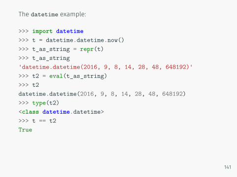
The datetime example:

>>> import datetime>>> t = datetime.datetime.now()>>> t_as_string = repr(t)>>> t_as_string'datetime.datetime(2016, 9, 8, 14, 28, 48, 648192)'>>> t2 = eval(t_as_string)>>> t2datetime.datetime(2016, 9, 8, 14, 28, 48, 648192)>>> type(t2)<class datetime.datetime>>>> t == t2True

141

Higher Order Functions

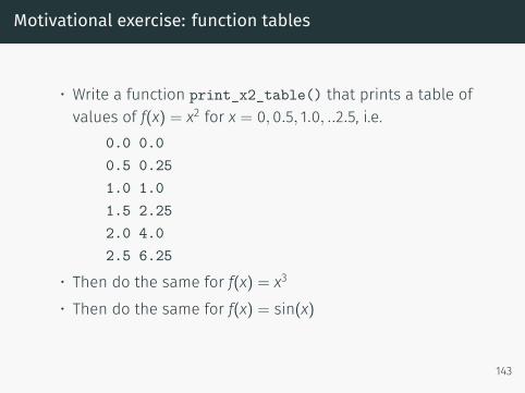
Motivational exercise: function tables

• Write a function print_x2_table() that prints a table ofvalues of f(x) = x2 for x = 0, 0.5, 1.0, ..2.5, i.e.

0.0 0.00.5 0.251.0 1.01.5 2.252.0 4.02.5 6.25

• Then do the same for f(x) = x3

• Then do the same for f(x) = sin(x)

143

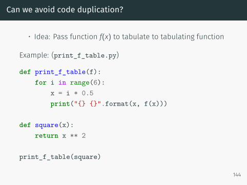
Can we avoid code duplication?

• Idea: Pass function f(x) to tabulate to tabulating function

Example: (print_f_table.py)

def print_f_table(f):for i in range(6):

x = i * 0.5print("{} {}".format(x, f(x)))

def square(x):return x ** 2

print_f_table(square)

144

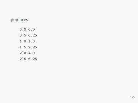
produces

0.0 0.00.5 0.251.0 1.01.5 2.252.0 4.02.5 6.25

145

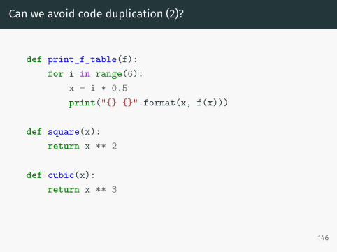
Can we avoid code duplication (2)?

def print_f_table(f):for i in range(6):

x = i * 0.5print("{} {}".format(x, f(x)))

def square(x):return x ** 2

def cubic(x):return x ** 3

146

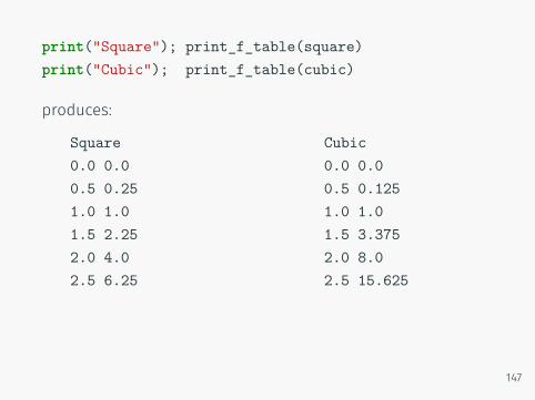
print("Square"); print_f_table(square)print("Cubic"); print_f_table(cubic)

produces:

Square0.0 0.00.5 0.251.0 1.01.5 2.252.0 4.02.5 6.25

Cubic0.0 0.00.5 0.1251.0 1.01.5 3.3752.0 8.02.5 15.625

147

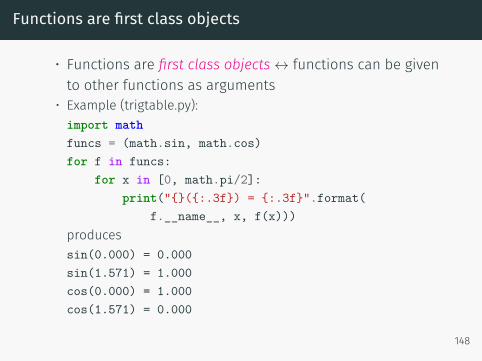
Functions are first class objects

• Functions are first class objects↔ functions can be givento other functions as arguments

• Example (trigtable.py):import mathfuncs = (math.sin, math.cos)for f in funcs:

for x in [0, math.pi/2]:print("{}({:.3f}) = {:.3f}".format(

f.__name__, x, f(x)))producessin(0.000) = 0.000sin(1.571) = 1.000cos(0.000) = 1.000cos(1.571) = 0.000

148

148

Modules

Writing module files

• Motivation: it is useful to bundle functions that are usedrepeatedly and belong to the same subject area into onemodule file (also called “library”)

• Every Python file can be imported as a module.• If this module file has a main program, then this isexecuted when the file is imported. This can be desiredbut sometimes it is not.

• We describe how a main program can be written which isonly executed if the file is run on its own but not if isimported as a library.

150

The internal __name__ variable (1)

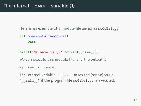
• Here is an example of a module file saved as module1.py:

def someusefulfunction():pass

print("My name is {}".format(__name__))

We can execute this module file, and the output is

My name is __main__

• The internal variable __name__ takes the (string) value"__main__" if the program file module1.py is executed.

151

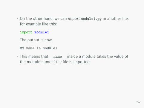
• On the other hand, we can import module1.py in another file,for example like this:

import module1

The output is now:

My name is module1

• This means that __name__ inside a module takes the value ofthe module name if the file is imported.

152

The internal __name__ variable (2)

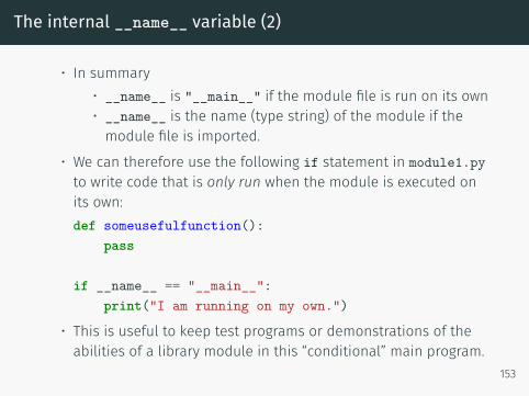
• In summary• __name__ is "__main__" if the module file is run on its own• __name__ is the name (type string) of the module if themodule file is imported.

• We can therefore use the following if statement in module1.pyto write code that is only run when the module is executed onits own:def someusefulfunction():

pass

if __name__ == "__main__":print("I am running on my own.")

• This is useful to keep test programs or demonstrations of theabilities of a library module in this “conditional” main program.

153

Library file example

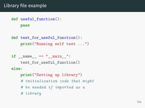
def useful_function():pass

def test_for_useful_function():print("Running self test ...")

if __name__ == "__main__":test_for_useful_function()

else:print("Setting up library")# initialisation code that might# be needed if imported as a# library

154

Default arguments

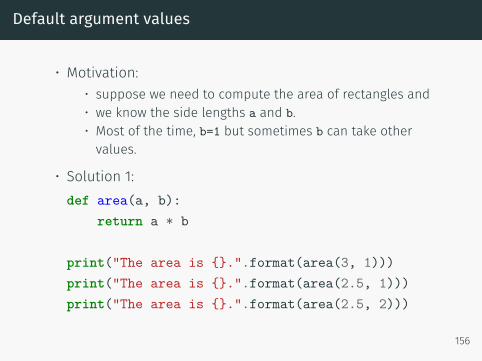
Default argument values

• Motivation:• suppose we need to compute the area of rectangles and• we know the side lengths a and b.• Most of the time, b=1 but sometimes b can take othervalues.

• Solution 1:def area(a, b):

return a * b

print("The area is {}.".format(area(3, 1)))print("The area is {}.".format(area(2.5, 1)))print("The area is {}.".format(area(2.5, 2)))

156

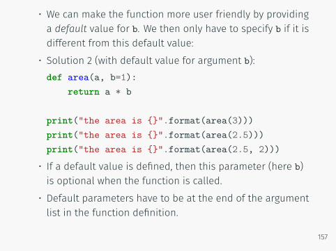
• We can make the function more user friendly by providinga default value for b. We then only have to specify b if it isdifferent from this default value:

• Solution 2 (with default value for argument b):def area(a, b=1):

return a * b

print("the area is {}".format(area(3)))print("the area is {}".format(area(2.5)))print("the area is {}".format(area(2.5, 2)))

• If a default value is defined, then this parameter (here b)is optional when the function is called.

• Default parameters have to be at the end of the argumentlist in the function definition.

157

Keyword argument values

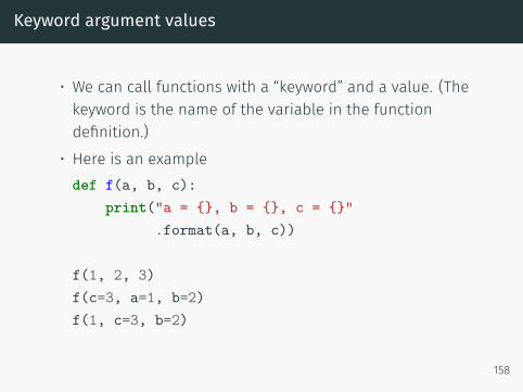
• We can call functions with a “keyword” and a value. (Thekeyword is the name of the variable in the functiondefinition.)

• Here is an exampledef f(a, b, c):

print("a = {}, b = {}, c = {}".format(a, b, c))

f(1, 2, 3)f(c=3, a=1, b=2)f(1, c=3, b=2)

158

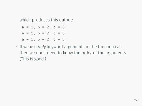
which produces this output:a = 1, b = 2, c = 3a = 1, b = 2, c = 3a = 1, b = 2, c = 3

• If we use only keyword arguments in the function call,then we don’t need to know the order of the arguments.(This is good.)

159

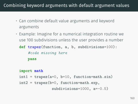
Combining keyword arguments with default argument values

• Can combine default value arguments and keywordarguments

• Example: Imagine for a numerical integration routine weuse 100 subdivisions unless the user provides a numberdef trapez(function, a, b, subdivisions=100):

#code missing herepass

import mathint1 = trapez(a=0, b=10, function=math.sin)int2 = trapez(b=0, function=math.exp,

subdivisions=1000, a=-0.5)

160

• Note that choosing meaningful variable names in thefunction definition makes the function more user friendly.

• You may have met default arguments in use before, forexample

• the open function uses mode='r' as a default value• the print function uses end='\n' as a default value

LAB6

161

161

Namespaces

Name spaces — what can be seen where?

• We distinguish between• global variables (defined in main program) and• local variables (defined for example in functions)• built-in functions

• The same variable name can be used in a function and inthe main program but they can refer to different objectsand do not interfere:

163

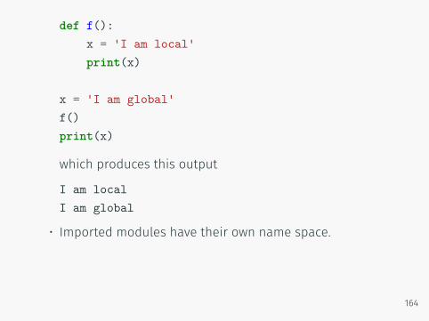
def f():x = 'I am local'print(x)

x = 'I am global'f()print(x)

which produces this output

I am localI am global

• Imported modules have their own name space.

164

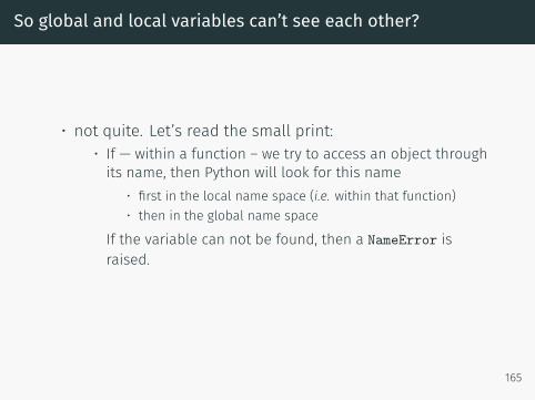
So global and local variables can’t see each other?

• not quite. Let’s read the small print:• If — within a function – we try to access an object throughits name, then Python will look for this name

• first in the local name space (i.e. within that function)• then in the global name space

If the variable can not be found, then a NameError israised.

165

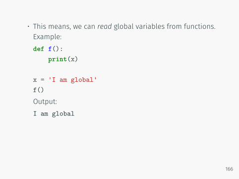
• This means, we can read global variables from functions.Example:def f():

print(x)

x = 'I am global'f()Output:I am global

166

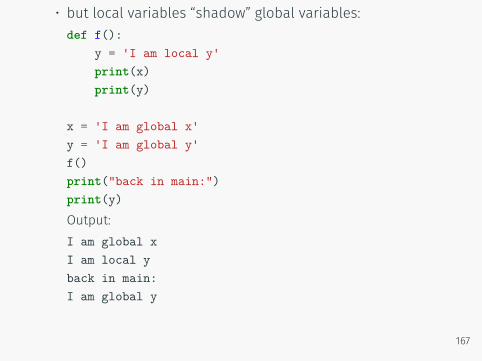
• but local variables “shadow” global variables:def f():

y = 'I am local y'print(x)print(y)

x = 'I am global x'y = 'I am global y'f()print("back in main:")print(y)Output:I am global xI am local yback in main:I am global y

167

• To modify global variables within a local namespace, weneed to use the global keyword.(This is not recommended so we won’t explain it. See also next slide.)

168

Why should I care about global variables?

• Generally, the use of global variables is notrecommended:

• functions should take all necessary input as argumentsand

• return all relevant output.• This makes the functions work as independent moduleswhich is good engineering practice and essential to controlcomplexity of software.

• However, sometimes the same constant or variable (suchas the mass of an object) is required throughout aprogram:

169

• it is not good practice to define this variable more thanonce (it is likely that we assign different values and getinconsistent results)

• in this case — in small programs — the use of (read-only)global variables may be acceptable.

• Object Oriented Programming provides a somewhat neatersolution to this.

170

Python’s look up rule

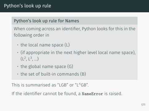
Python’s look up rule for NamesWhen coming across an identifier, Python looks for this in thefollowing order in

• the local name space (L)• (if appropriate in the next higher level local name space),(L2, L3, …)

• the global name space (G)• the set of built-in commands (B)

This is summarised as “LGB” or “LnGB”.

If the identifier cannot be found, a NameError is raised.

171

Python IDEs

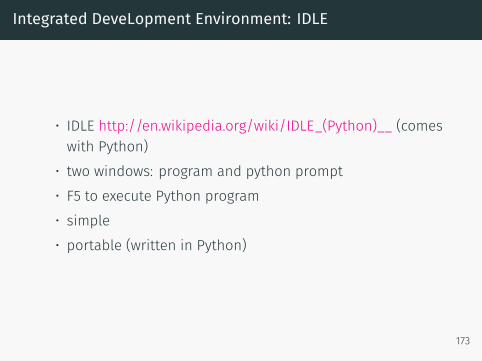
Integrated DeveLopment Environment: IDLE

• IDLE http://en.wikipedia.org/wiki/IDLE_(Python)__ (comeswith Python)

• two windows: program and python prompt• F5 to execute Python program• simple• portable (written in Python)

173

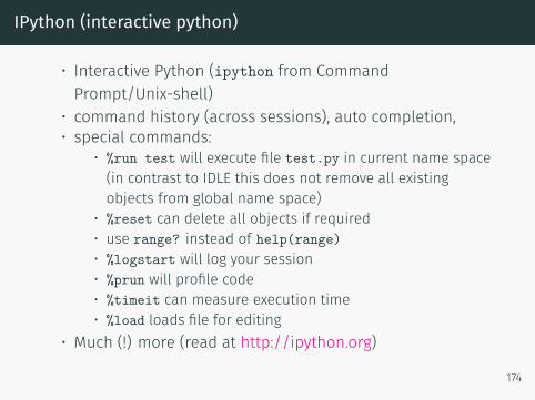
IPython (interactive python)

• Interactive Python (ipython from CommandPrompt/Unix-shell)

• command history (across sessions), auto completion,• special commands:

• %run test will execute file test.py in current name space(in contrast to IDLE this does not remove all existingobjects from global name space)

• %reset can delete all objects if required• use range? instead of help(range)• %logstart will log your session• %prun will profile code• %timeit can measure execution time• %load loads file for editing

• Much (!) more (read at http://ipython.org)

174

IPython’s QT console

• Prompt as IPython (with all it’s features): running in agraphics console rather than in text console

• can inline matplotlib figures• Read more at http://ipython.org/ipython-doc/dev/interactive/qtconsole.html

175

Jupyter Notebook

• Used to be the IPython Notebook, but now supports manymore languages than Python, thus a new name waschosen.

• Jupyter Notebook creates an executable document that ishosted in a web browser.

• We recommend you try this at some point, it has greatvalue for computational engineering and research.

• Read more at http://jupyter.org

176

... and many others

Including

• Eclipse• Spyder• PyCharm (commercial)• Emacs• vi, vim• Sublime Text (commercial)• Kate

177

List comprehension

List comprehension

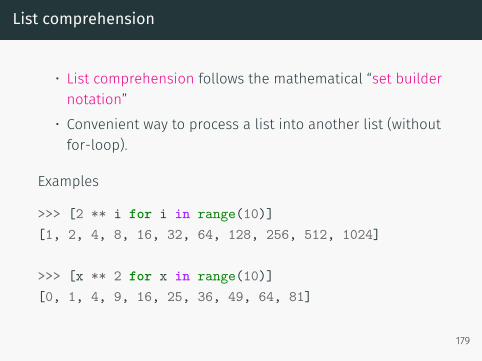
• List comprehension follows the mathematical “set buildernotation”

• Convenient way to process a list into another list (withoutfor-loop).

Examples

>>> [2 ** i for i in range(10)][1, 2, 4, 8, 16, 32, 64, 128, 256, 512, 1024]

>>> [x ** 2 for x in range(10)][0, 1, 4, 9, 16, 25, 36, 49, 64, 81]

179

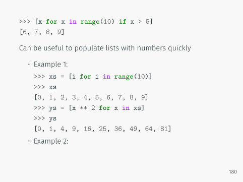
>>> [x for x in range(10) if x > 5][6, 7, 8, 9]

Can be useful to populate lists with numbers quickly

• Example 1:>>> xs = [i for i in range(10)]>>> xs[0, 1, 2, 3, 4, 5, 6, 7, 8, 9]>>> ys = [x ** 2 for x in xs]>>> ys[0, 1, 4, 9, 16, 25, 36, 49, 64, 81]

• Example 2:

180

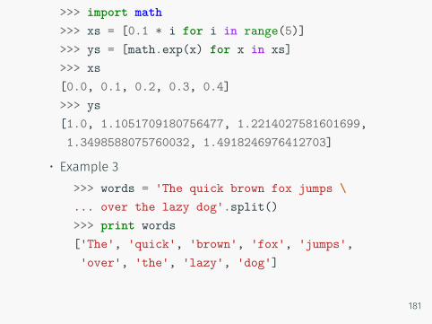
>>> import math>>> xs = [0.1 * i for i in range(5)]>>> ys = [math.exp(x) for x in xs]>>> xs[0.0, 0.1, 0.2, 0.3, 0.4]>>> ys[1.0, 1.1051709180756477, 1.2214027581601699,1.3498588075760032, 1.4918246976412703]

• Example 3>>> words = 'The quick brown fox jumps \... over the lazy dog'.split()>>> print words['The', 'quick', 'brown', 'fox', 'jumps','over', 'the', 'lazy', 'dog']

181

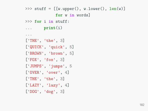
>>> stuff = [[w.upper(), w.lower(), len(w)]for w in words]

>>> for i in stuff:... print(i)...['THE', 'the', 3]['QUICK', 'quick', 5]['BROWN', 'brown', 5]['FOX', 'fox', 3]['JUMPS', 'jumps', 5['OVER', 'over', 4]['THE', 'the', 3]['LAZY', 'lazy', 4]['DOG', 'dog', 3]

182

List comprehension with conditional

• Can extend list comprehension syntax with if CONDITIONto include only elements for which CONDITION is true.

• Example:>>> [i for i in range(10)][0, 1, 2, 3, 4, 5, 6, 7, 8, 9]

>>> [i for i in range(10) if i > 5][6, 7, 8, 9]

>>> [i for i in range(10) if i ** 2 > 5][3, 4, 5, 6, 7, 8, 9]

183

Dictionaries

Dictionaries

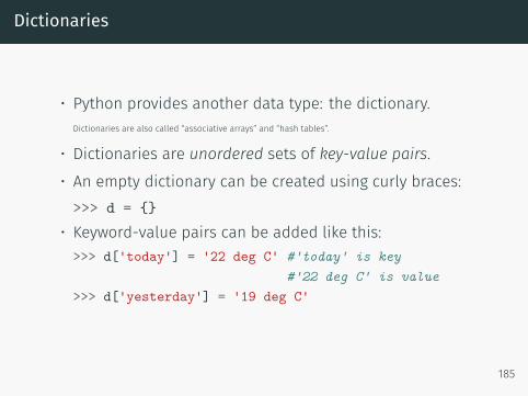
• Python provides another data type: the dictionary.Dictionaries are also called “associative arrays” and “hash tables”.

• Dictionaries are unordered sets of key-value pairs.• An empty dictionary can be created using curly braces:>>> d = {}

• Keyword-value pairs can be added like this:>>> d['today'] = '22 deg C' #'today' is key

#'22 deg C' is value>>> d['yesterday'] = '19 deg C'

185

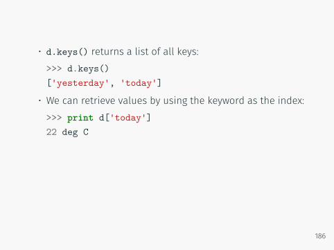
• d.keys() returns a list of all keys:>>> d.keys()['yesterday', 'today']

• We can retrieve values by using the keyword as the index:>>> print d['today']22 deg C

186

Dictionary example 1

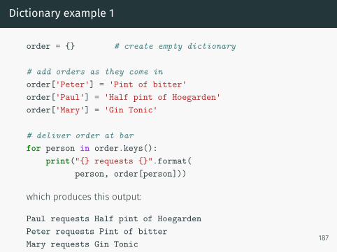
order = {} # create empty dictionary

# add orders as they come inorder['Peter'] = 'Pint of bitter'order['Paul'] = 'Half pint of Hoegarden'order['Mary'] = 'Gin Tonic'

# deliver order at barfor person in order.keys():

print("{} requests {}".format(person, order[person]))

which produces this output:

Paul requests Half pint of HoegardenPeter requests Pint of bitterMary requests Gin Tonic

187

Dictionary

Some more technicalities:

• The dictionary key can be any (immutable) Python object.This includes:

• numbers• strings• tuples.

• dictionaries are very fast in retrieving values (when giventhe key)

188

Dictionary use case

• What are dictionnaries good for? Consider this example:

dic = {}dic["Andy C"] = "room 1031"dic["Ken"] = "room 1027"dic["Hans"] = "room 1033"

for key in dic.keys():print("{} works in {}"

.format(key, dic[key]))

Output:

Hans works in room 1033Andy C works in room 1031Ken works in room 1027

189

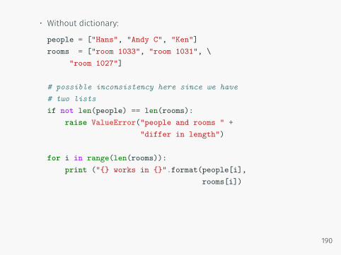
• Without dictionary:

people = ["Hans", "Andy C", "Ken"]rooms = ["room 1033", "room 1031", \

"room 1027"]

# possible inconsistency here since we have# two listsif not len(people) == len(rooms):

raise ValueError("people and rooms " +"differ in length")

for i in range(len(rooms)):print ("{} works in {}".format(people[i],

rooms[i])

190

Iterating over dictionaries

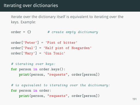
Iterate over the dictionary itself is equivalent to iterating over thekeys. Example:

order = {} # create empty dictionary

order['Peter'] = 'Pint of bitter'order['Paul'] = 'Half pint of Hoegarden'order['Mary'] = 'Gin Tonic'

# iterating over keys:for person in order.keys():

print(person, "requests", order[person])

# is equivalent to iterating over the dictionary:for person in order:

print(person, "requests", order[person])191

Summary dictionaries

What to remember:

• Python provides dictionaries• very powerful construct• a bit like a data base (and values can be dictionaryobjects)

• fast to retrieve value• likely to be useful if you are dealing with two lists at thesame time (possibly one of them contains the keywordand the other the value)

• useful if you have a data set that needs to be indexed bystrings or tuples (or other immutable objects)

192

192

Recursion

Recursion

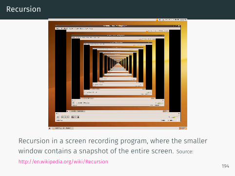
Recursion in a screen recording program, where the smallerwindow contains a snapshot of the entire screen. Source:http://en.wikipedia.org/wiki/Recursion

194

Recursion example: factorial

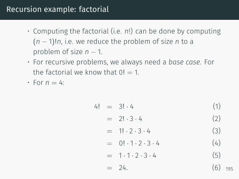
• Computing the factorial (i.e. n!) can be done by computing(n− 1)!n, i.e. we reduce the problem of size n to aproblem of size n− 1.

• For recursive problems, we always need a base case. Forthe factorial we know that 0! = 1.

• For n = 4:

4! = 3! · 4 (1)= 2! · 3 · 4 (2)= 1! · 2 · 3 · 4 (3)= 0! · 1 · 2 · 3 · 4 (4)= 1 · 1 · 2 · 3 · 4 (5)= 24. (6) 195

Recursion example

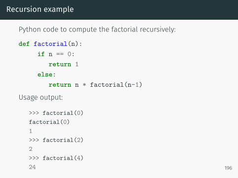
Python code to compute the factorial recursively:

def factorial(n):if n == 0:

return 1else:

return n * factorial(n-1)

Usage output:

>>> factorial(0)factorial(0)1>>> factorial(2)2>>> factorial(4)24 196

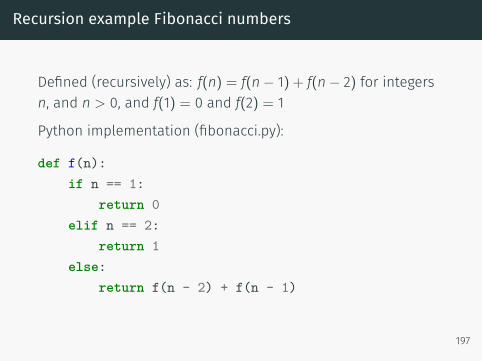
Recursion example Fibonacci numbers

Defined (recursively) as: f(n) = f(n− 1) + f(n− 2) for integersn, and n > 0, and f(1) = 0 and f(2) = 1

Python implementation (fibonacci.py):

def f(n):if n == 1:

return 0elif n == 2:

return 1else:

return f(n - 2) + f(n - 1)

197

Recursion exercises

1. Write a function recsum(n) that sums the numbers from 1to n recursively

2. Study the recursive Fibonacci function from slide 197:• what is the largest number n for which we can reasonablecompute f(n) within a minute?

• Can you write faster versions of the Fibonacci function?(There are faster versions with and without recursion.)

198

Common Computational Tasks

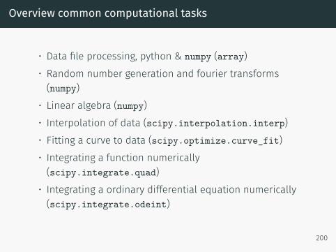
Overview common computational tasks

• Data file processing, python & numpy (array)• Random number generation and fourier transforms(numpy)

• Linear algebra (numpy)• Interpolation of data (scipy.interpolation.interp)• Fitting a curve to data (scipy.optimize.curve_fit)• Integrating a function numerically(scipy.integrate.quad)

• Integrating a ordinary differential equation numerically(scipy.integrate.odeint)

200

• Finding the root of a function (scipy.optimize.fsolve,scipy.optimize.brentq)

• Minimising a function (scipy.optimize.fmin)

• Symbolic manipulation of terms, including integration,differentiation and code generation (sympy)

• Data analytics (pandas)

201

201

Root finding

Rootfinding

Root findingGiven a function f(x), we are searching an x0 so f(x0) = 0. Wecall x0 a root of f(x).

Why?

• Often need to know when a particular function reaches avalue, for example the water temperature T(t) reaching373 K. In that case, we define

f(t) = T(t)− 373

and search the root t0 for f(t)

We introduce two methods:

• Bisection method• Newton method 203

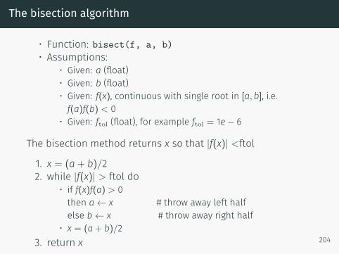
The bisection algorithm

• Function: bisect(f, a, b)• Assumptions:

• Given: a (float)• Given: b (float)• Given: f(x), continuous with single root in [a,b], i.e.f(a)f(b) < 0

• Given: ftol (float), for example ftol = 1e− 6

The bisection method returns x so that |f(x)| <ftol

1. x = (a+ b)/22. while |f(x)| > ftol do

• if f(x)f(a) > 0then a← x # throw away left halfelse b← x # throw away right half

• x = (a+ b)/23. return x 204

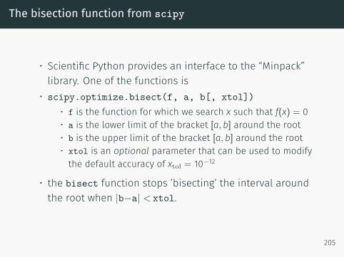
The bisection function from scipy

• Scientific Python provides an interface to the “Minpack”library. One of the functions is

• scipy.optimize.bisect(f, a, b[, xtol])• f is the function for which we search x such that f(x) = 0• a is the lower limit of the bracket [a,b] around the root• b is the upper limit of the bracket [a,b] around the root• xtol is an optional parameter that can be used to modifythe default accuracy of xtol = 10−12

• the bisect function stops ’bisecting’ the interval aroundthe root when |b−a| < xtol.

205

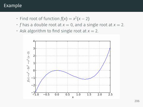
Example

• Find root of function f(x) = x2(x− 2)• f has a double root at x = 0, and a single root at x = 2.• Ask algorithm to find single root at x = 2.

1.0 0.5 0.0 0.5 1.0 1.5 2.0 2.5x

3

2

1

0

1

2

3

4

f(x)=x

3−

2x2

=x

2(x−

2)

206

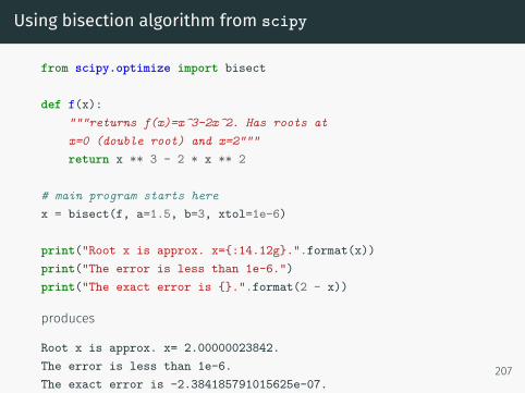
Using bisection algorithm from scipy

from scipy.optimize import bisect

def f(x):"""returns f(x)=x^3-2x^2. Has roots atx=0 (double root) and x=2"""return x ** 3 - 2 * x ** 2

# main program starts herex = bisect(f, a=1.5, b=3, xtol=1e-6)

print("Root x is approx. x={:14.12g}.".format(x))print("The error is less than 1e-6.")print("The exact error is {}.".format(2 - x))

produces

Root x is approx. x= 2.00000023842.The error is less than 1e-6.The exact error is -2.384185791015625e-07.

207

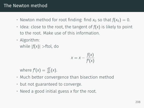
The Newton method

• Newton method for root finding: find x0 so that f(x0) = 0.• Idea: close to the root, the tangent of f(x) is likely to pointto the root. Make use of this information.

• Algorithm:while |f(x)| >ftol, do

x = x− f(x)f′(x)

where f′(x) = dfdx(x).

• Much better convergence than bisection method• but not guaranteed to converge.• Need a good initial guess x for the root.

208

Using Newton algorithm from scipy

from scipy.optimize import newton

def f(x):"""returns f(x)=x^3-2x^2. Has roots atx=0 (double root) and x=2"""return x ** 3 - 2 * x ** 2

# main program starts herex = newton(f, x0=1.6)

print("Root x is approx. x={:14.12g}.".format(x))print("The error is less than 1e-6.")print("The exact error is {}.".format(2 - x))

produces

Root x is approx. x= 2.The error is less than 1e-6.The exact error is 9.769962616701378e-15.

209

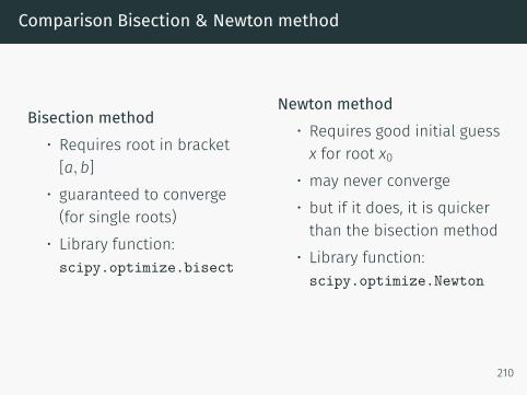
Comparison Bisection & Newton method

Bisection method• Requires root in bracket[a,b]

• guaranteed to converge(for single roots)

• Library function:scipy.optimize.bisect

Newton method• Requires good initial guessx for root x0

• may never converge• but if it does, it is quickerthan the bisection method

• Library function:scipy.optimize.Newton

210

Root finding summary

• Given the function f(x), applications for root findinginclude:

• to find x1 so that f(x1) = y for a given y (this is equivalent tocomputing the inverse of the function f).

• to find crossing point xc of two functions f1(x) and f2(x) (byfinding root of difference function g(x) = f1(x)− f2(x))

• Recommended method: scipy.optimize.brentq whichcombines the safe feature of the bisect method with thespeed of the Newton method.

• For multi-dimensional functions f(x), usescipy.optimize.fsolve.

211

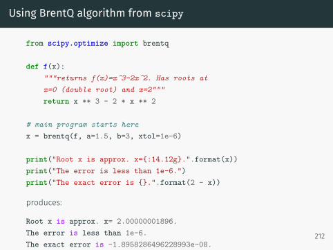
Using BrentQ algorithm from scipy

from scipy.optimize import brentq

def f(x):"""returns f(x)=x^3-2x^2. Has roots atx=0 (double root) and x=2"""return x ** 3 - 2 * x ** 2

# main program starts herex = brentq(f, a=1.5, b=3, xtol=1e-6)

print("Root x is approx. x={:14.12g}.".format(x))print("The error is less than 1e-6.")print("The exact error is {}.".format(2 - x))

produces:

Root x is approx. x= 2.00000001896.The error is less than 1e-6.The exact error is -1.8958286496228993e-08.

212

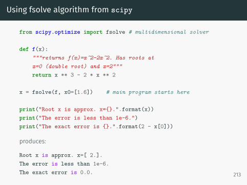
Using fsolve algorithm from scipy

from scipy.optimize import fsolve # multidimensional solver

def f(x):"""returns f(x)=x^2-2x^2. Has roots atx=0 (double root) and x=2"""return x ** 3 - 2 * x ** 2

x = fsolve(f, x0=[1.6]) # main program starts here

print("Root x is approx. x={}.".format(x))print("The error is less than 1e-6.")print("The exact error is {}.".format(2 - x[0]))

produces:

Root x is approx. x=[ 2.].The error is less than 1e-6.The exact error is 0.0. 213

Derivatives

Overview

• Motivation:

• We need derivatives of functions for some optimisationand root finding algorithms

• Not always is the function analytically known (but we areusually able to compute the function numerically)

• The material presented here forms the basis of thefinite-difference technique that is commonly used to solveordinary and partial differential equations.

• The following slides show

• the forward difference technique• the backward difference technique and the

215

• central difference technique to approximate the derivativeof a function.

• We also derive the accuracy of each of these methods.

216

The 1st derivative

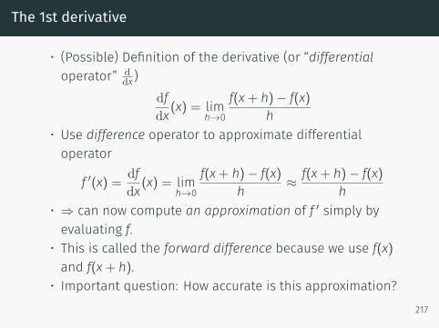
• (Possible) Definition of the derivative (or “differentialoperator” d

dx )dfdx(x) = lim

h→0

f(x+ h)− f(x)h

• Use difference operator to approximate differentialoperator

f ′(x) = dfdx(x) = lim

h→0

f(x+ h)− f(x)h ≈ f(x+ h)− f(x)

h• ⇒ can now compute an approximation of f ′ simply byevaluating f.

• This is called the forward difference because we use f(x)and f(x+ h).

• Important question: How accurate is this approximation?217

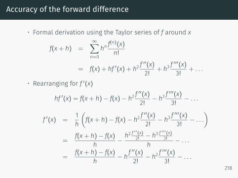
Accuracy of the forward difference

• Formal derivation using the Taylor series of f around x

f(x+ h) =∞∑n=0

hn f(n)(x)n!

= f(x) + hf ′(x) + h2 f′′(x)2! + h3 f

′′′(x)3! + . . .

• Rearranging for f ′(x)

hf ′(x) = f(x+ h)− f(x)− h2 f′′(x)2! − h3 f

′′′(x)3! − . . .

f ′(x) =1h

(f(x+ h)− f(x)− h2 f

′′(x)2! − h3 f

′′′(x)3! − . . .

)=

f(x+ h)− f(x)h −

h2 f′′(x)2! − h

3 f ′′′(x)3!

h − . . .

=f(x+ h)− f(x)

h − hf′′(x)2! − h2 f

′′′(x)3! − . . .

218

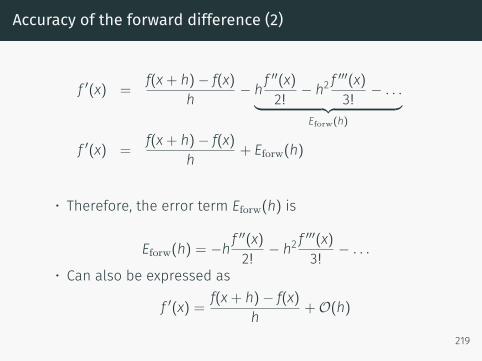
Accuracy of the forward difference (2)

f ′(x) =f(x+ h)− f(x)

h − hf′′(x)2! − h

2 f ′′′(x)3! − . . .︸ ︷︷ ︸

Eforw(h)

f ′(x) =f(x+ h)− f(x)

h + Eforw(h)

• Therefore, the error term Eforw(h) is

Eforw(h) = −hf ′′(x)2! − h

2 f ′′′(x)3! − . . .

• Can also be expressed as

f ′(x) = f(x+ h)− f(x)h +O(h)

219

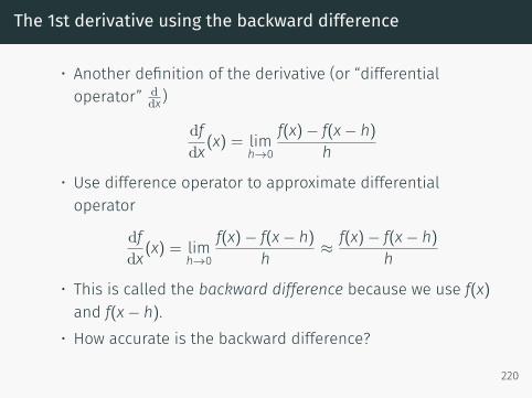
The 1st derivative using the backward difference

• Another definition of the derivative (or “differentialoperator” d

dx )

dfdx(x) = lim

h→0

f(x)− f(x− h)h

• Use difference operator to approximate differentialoperator

dfdx(x) = lim

h→0

f(x)− f(x− h)h ≈ f(x)− f(x− h)

h

• This is called the backward difference because we use f(x)and f(x− h).

• How accurate is the backward difference?

220

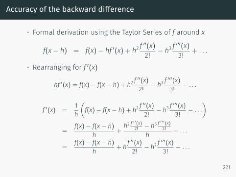
Accuracy of the backward difference

• Formal derivation using the Taylor Series of f around x

f(x− h) = f(x)− hf ′(x) + h2 f′′(x)2! − h

3 f ′′′(x)3! + . . .

• Rearranging for f ′(x)

hf ′(x) = f(x)− f(x− h) + h2 f′′(x)2! − h3 f

′′′(x)3! − . . .

f ′(x) =1h

(f(x)− f(x− h) + h2 f

′′(x)2! − h3 f

′′′(x)3! − . . .

)=

f(x)− f(x− h)h +

h2 f′′(x)2! − h

3 f ′′′(x)3!

h − . . .

=f(x)− f(x− h)

h + hf′′(x)2! − h2 f

′′′(x)3! − . . .

221

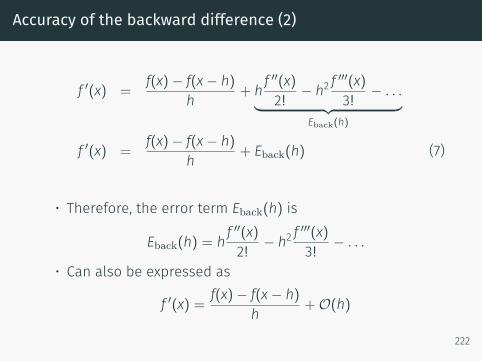
Accuracy of the backward difference (2)

f ′(x) =f(x)− f(x− h)

h + hf′′(x)2! − h

2 f ′′′(x)3! − . . .︸ ︷︷ ︸

Eback(h)

f ′(x) =f(x)− f(x− h)

h + Eback(h) (7)

• Therefore, the error term Eback(h) is

Eback(h) = hf′′(x)2! − h

2 f ′′′(x)3! − . . .

• Can also be expressed as

f ′(x) = f(x)− f(x− h)h +O(h)

222

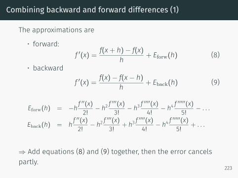
Combining backward and forward differences (1)

The approximations are

• forward:f ′(x) = f(x+ h)− f(x)

h + Eforw(h) (8)

• backward

f ′(x) = f(x)− f(x− h)h + Eback(h) (9)

Eforw(h) = −hf′′(x)2! − h2 f

′′′(x)3! − h3 f

′′′′(x)4! − h4 f

′′′′′(x)5! − . . .

Eback(h) = hf′′(x)2! − h2 f

′′′(x)3! + h3 f

′′′′(x)4! − h4 f

′′′′′(x)5! + . . .

⇒ Add equations (8) and (9) together, then the error cancelspartly.

223

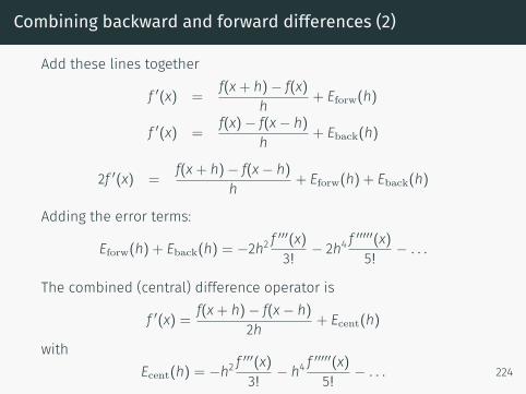
Combining backward and forward differences (2)

Add these lines together

f ′(x) =f(x+ h)− f(x)

h + Eforw(h)

f ′(x) =f(x)− f(x− h)

h + Eback(h)

2f ′(x) =f(x+ h)− f(x− h)

h + Eforw(h) + Eback(h)

Adding the error terms:

Eforw(h) + Eback(h) = −2h2f ′′′(x)3! − 2h4 f

′′′′′(x)5! − . . .

The combined (central) difference operator is

f ′(x) = f(x+ h)− f(x− h)2h + Ecent(h)

withEcent(h) = −h2

f ′′′(x)3! − h4 f

′′′′′(x)5! − . . . 224

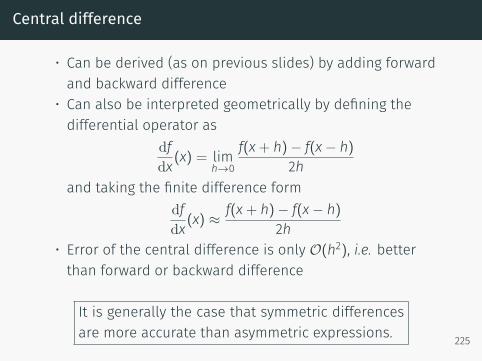
Central difference

• Can be derived (as on previous slides) by adding forwardand backward difference

• Can also be interpreted geometrically by defining thedifferential operator as

dfdx(x) = lim

h→0

f(x+ h)− f(x− h)2h

and taking the finite difference formdfdx(x) ≈

f(x+ h)− f(x− h)2h

• Error of the central difference is only O(h2), i.e. betterthan forward or backward difference

It is generally the case that symmetric differencesare more accurate than asymmetric expressions. 225

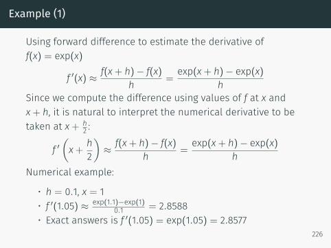
Example (1)

Using forward difference to estimate the derivative off(x) = exp(x)

f ′(x) ≈ f(x+ h)− f(x)h =

exp(x+ h)− exp(x)h

Since we compute the difference using values of f at x andx+ h, it is natural to interpret the numerical derivative to betaken at x+ h

2 :

f ′(x+ h

2

)≈ f(x+ h)− f(x)

h =exp(x+ h)− exp(x)

hNumerical example:

• h = 0.1, x = 1• f ′(1.05) ≈ exp(1.1)−exp(1)

0.1 = 2.8588• Exact answers is f ′(1.05) = exp(1.05) = 2.8577

226

Example (2)

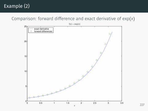
Comparison: forward difference and exact derivative of exp(x)

0 0.5 1 1.5 2 2.5 3 3.50

5

10

15

20

25f(x) = exp(x)

x

exact derivativeforward differences

227

Summary

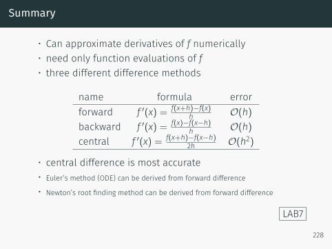
• Can approximate derivatives of f numerically• need only function evaluations of f• three different difference methods

name formula errorforward f ′(x) = f(x+h)−f(x)

h O(h)backward f ′(x) = f(x)−f(x−h)

h O(h)central f ′(x) = f(x+h)−f(x−h)

2h O(h2)

• central difference is most accurate• Euler’s method (ODE) can be derived from forward difference

• Newton’s root finding method can be derived from forward difference

LAB7

228

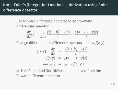
Note: Euler’s (integration) method — derivation using finitedifference operator

• Use forward difference operator to approximatedifferential operator

dydx(x) = lim

h→0

y(x+ h)− y(x)h ≈ y(x+ h)− y(x)

h• Change differential to difference operator in dy

dx = f(x, y)

f(x, y) = dydx ≈ y(x+ h)− y(x)

hhf(x, y) ≈ y(x+ h)− y(x)=⇒ yi+1 = yi + hf(xi, yi)

• ⇒ Euler’s method (for ODEs) can be derived from theforward difference operator.

229

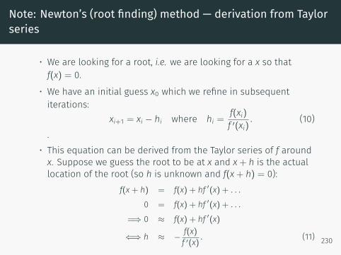
Note: Newton’s (root finding) method — derivation from Taylorseries

• We are looking for a root, i.e. we are looking for a x so thatf(x) = 0.

• We have an initial guess x0 which we refine in subsequentiterations:

xi+1 = xi − hi where hi =f(xi)f ′(xi)

. (10).

• This equation can be derived from the Taylor series of f aroundx. Suppose we guess the root to be at x and x+ h is the actuallocation of the root (so h is unknown and f(x+ h) = 0):

f(x+ h) = f(x) + hf ′(x) + . . .

0 = f(x) + hf ′(x) + . . .

=⇒ 0 ≈ f(x) + hf ′(x)

⇐⇒ h ≈ − f(x)f ′(x) . (11) 230

230

Numpy

numpy

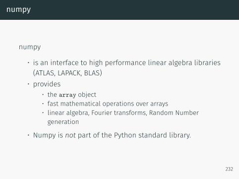
numpy

• is an interface to high performance linear algebra libraries(ATLAS, LAPACK, BLAS)

• provides• the array object• fast mathematical operations over arrays• linear algebra, Fourier transforms, Random Numbergeneration

• Numpy is not part of the Python standard library.

232

numpy arrays (vectors)

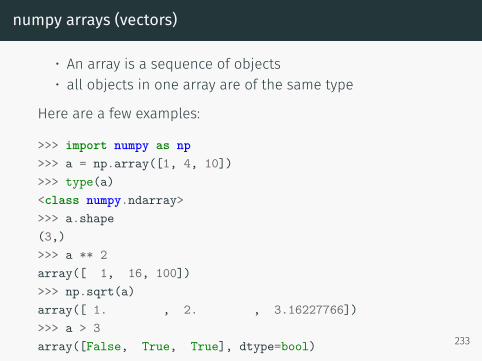
• An array is a sequence of objects• all objects in one array are of the same type

Here are a few examples:

>>> import numpy as np>>> a = np.array([1, 4, 10])>>> type(a)<class numpy.ndarray>>>> a.shape(3,)>>> a ** 2array([ 1, 16, 100])>>> np.sqrt(a)array([ 1. , 2. , 3.16227766])>>> a > 3array([False, True, True], dtype=bool) 233

Array creation

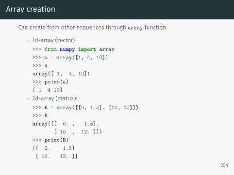
Can create from other sequences through array function:

• 1d-array (vector)>>> from numpy import array>>> a = array([1, 4, 10])>>> aarray([ 1, 4, 10])>>> print(a)[ 1 4 10]

• 2d-array (matrix):>>> B = array([[0, 1.5], [10, 12]])>>> Barray([[ 0. , 1.5],

[ 10. , 12. ]])>>> print(B)[[ 0. 1.5][ 10. 12. ]]

234

Array shape

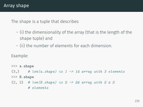
The shape is a tuple that describes

• (i) the dimensionality of the array (that is the length of theshape tuple) and

• (ii) the number of elements for each dimension.

Example:

>>> a.shape(3,) # len(a.shape) is 1 -> 1d array with 3 elements>>> B.shape(2, 2) # len(B.shape) is 2 -> 2d array with 2 x 2

# elements

235

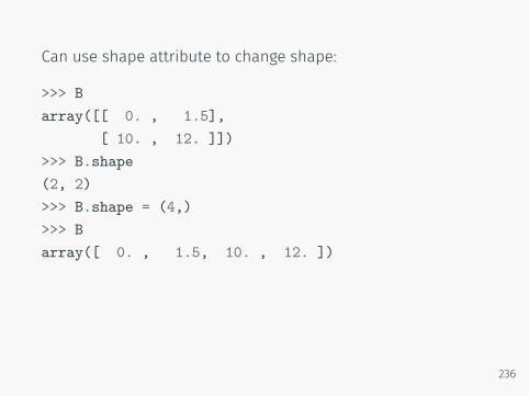
Can use shape attribute to change shape:

>>> Barray([[ 0. , 1.5],

[ 10. , 12. ]])>>> B.shape(2, 2)>>> B.shape = (4,)>>> Barray([ 0. , 1.5, 10. , 12. ])

236

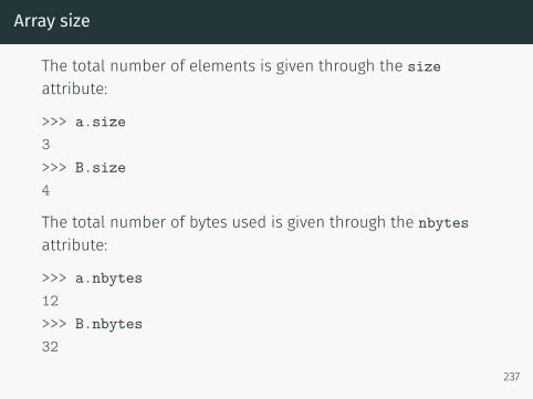
Array size

The total number of elements is given through the sizeattribute:

>>> a.size3>>> B.size4

The total number of bytes used is given through the nbytesattribute:

>>> a.nbytes12>>> B.nbytes32

237

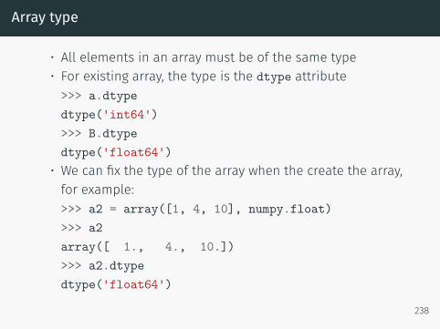
Array type

• All elements in an array must be of the same type• For existing array, the type is the dtype attribute>>> a.dtypedtype('int64')>>> B.dtypedtype('float64')

• We can fix the type of the array when the create the array,for example:>>> a2 = array([1, 4, 10], numpy.float)>>> a2array([ 1., 4., 10.])>>> a2.dtypedtype('float64')

238

Important array types

• For numerical calculations, we normally use double floatswhich are knows as float64 or short float in this text.:>>> a2 = array([1, 4, 10], numpy.float)>>> a2.dtypedtype('float64')

• This is also the default type for zeros and ones.• A full list is available athttp://docs.scipy.org/doc/numpy/user/basics.types.html

239

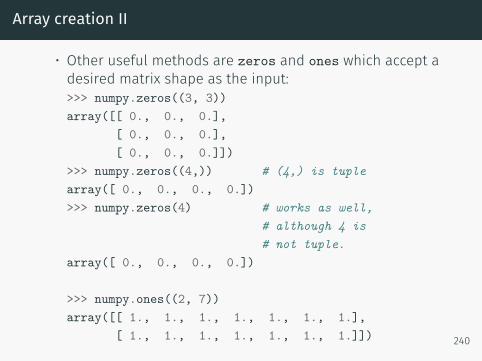
Array creation II

• Other useful methods are zeros and ones which accept adesired matrix shape as the input:>>> numpy.zeros((3, 3))array([[ 0., 0., 0.],

[ 0., 0., 0.],[ 0., 0., 0.]])

>>> numpy.zeros((4,)) # (4,) is tuplearray([ 0., 0., 0., 0.])>>> numpy.zeros(4) # works as well,

# although 4 is# not tuple.

array([ 0., 0., 0., 0.])

>>> numpy.ones((2, 7))array([[ 1., 1., 1., 1., 1., 1., 1.],

[ 1., 1., 1., 1., 1., 1., 1.]]) 240

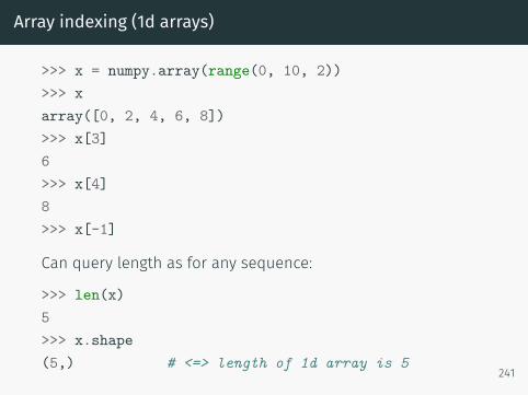
Array indexing (1d arrays)

>>> x = numpy.array(range(0, 10, 2))>>> xarray([0, 2, 4, 6, 8])>>> x[3]6>>> x[4]8>>> x[-1]

Can query length as for any sequence:

>>> len(x)5>>> x.shape(5,) # <=> length of 1d array is 5

241

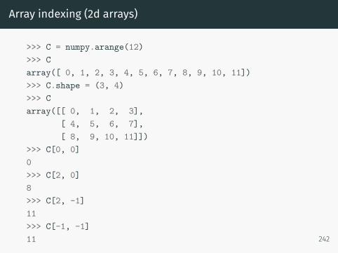
Array indexing (2d arrays)

>>> C = numpy.arange(12)>>> Carray([ 0, 1, 2, 3, 4, 5, 6, 7, 8, 9, 10, 11])>>> C.shape = (3, 4)>>> Carray([[ 0, 1, 2, 3],

[ 4, 5, 6, 7],[ 8, 9, 10, 11]])

>>> C[0, 0]0>>> C[2, 0]8>>> C[2, -1]11>>> C[-1, -1]11 242

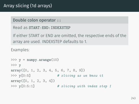
Array slicing (1d arrays)

Double colon operator ::

Read as START:END:INDEXSTEP

If either START or END are omitted, the respective ends of thearray are used. INDEXSTEP defaults to 1.

Examples:

>>> y = numpy.arange(10)>>> yarray([0, 1, 2, 3, 4, 5, 6, 7, 8, 9])>>> y[0:5] # slicing as we know itarray([0, 1, 2, 3, 4])>>> y[0:5:1] # slicing with index step 1

243

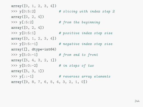
array([0, 1, 2, 3, 4])>>> y[0:5:2] # slicing with index step 2array([0, 2, 4])>>> y[:5:2] # from the beginningarray([0, 2, 4])>>> y[0:5:1] # positive index step sizearray([0, 1, 2, 3, 4])>>> y[0:5:-1] # negative index step sizearray([], dtype=int64)>>> y[5:0:-1] # from end to frontarray([5, 4, 3, 2, 1])>>> y[5:0:-2] # in steps of twoarray([5, 3, 1])>>> y[::-1] # reverses array elementsarray([9, 8, 7, 6, 5, 4, 3, 2, 1, 0])

244

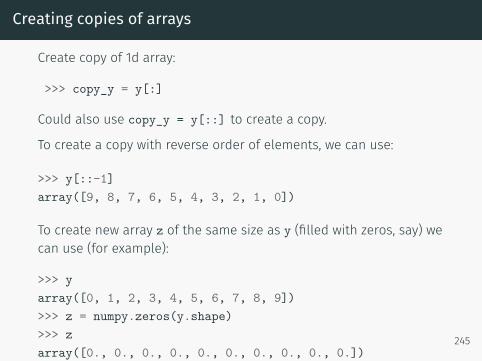
Creating copies of arrays

Create copy of 1d array:

>>> copy_y = y[:]

Could also use copy_y = y[::] to create a copy.

To create a copy with reverse order of elements, we can use:

>>> y[::-1]array([9, 8, 7, 6, 5, 4, 3, 2, 1, 0])

To create new array z of the same size as y (filled with zeros, say) wecan use (for example):

>>> yarray([0, 1, 2, 3, 4, 5, 6, 7, 8, 9])>>> z = numpy.zeros(y.shape)>>> zarray([0., 0., 0., 0., 0., 0., 0., 0., 0., 0.])

245

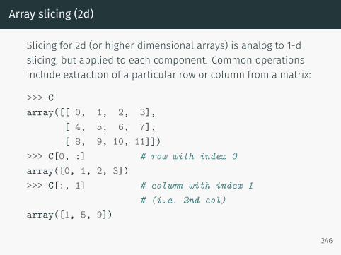
Array slicing (2d)

Slicing for 2d (or higher dimensional arrays) is analog to 1-dslicing, but applied to each component. Common operationsinclude extraction of a particular row or column from a matrix:

>>> Carray([[ 0, 1, 2, 3],

[ 4, 5, 6, 7],[ 8, 9, 10, 11]])

>>> C[0, :] # row with index 0array([0, 1, 2, 3])>>> C[:, 1] # column with index 1

# (i.e. 2nd col)array([1, 5, 9])

246

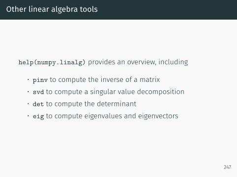
Other linear algebra tools

help(numpy.linalg) provides an overview, including

• pinv to compute the inverse of a matrix• svd to compute a singular value decomposition• det to compute the determinant• eig to compute eigenvalues and eigenvectors

247

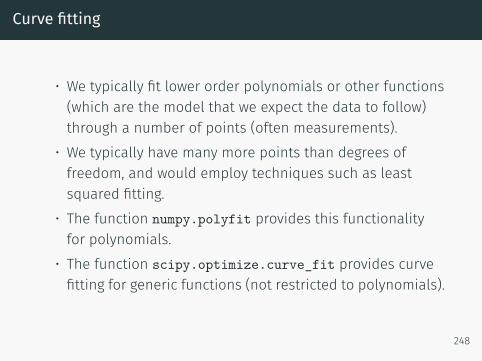
Curve fitting

• We typically fit lower order polynomials or other functions(which are the model that we expect the data to follow)through a number of points (often measurements).

• We typically have many more points than degrees offreedom, and would employ techniques such as leastsquared fitting.

• The function numpy.polyfit provides this functionalityfor polynomials.

• The function scipy.optimize.curve_fit provides curvefitting for generic functions (not restricted to polynomials).

248

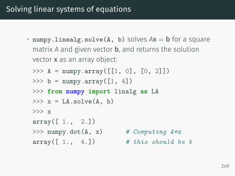
Solving linear systems of equations

• numpy.linealg.solve(A, b) solves Ax = b for a squarematrix A and given vector b, and returns the solutionvector x as an array object:>>> A = numpy.array([[1, 0], [0, 2]])>>> b = numpy.array([1, 4])>>> from numpy import linalg as LA>>> x = LA.solve(A, b)>>> xarray([ 1., 2.])>>> numpy.dot(A, x) # Computing A*xarray([ 1., 4.]) # this should be b

249

Other comments

• numpy provides fast array operations (comparable toMatlab’s matrices)

• fast if number of elements is large: for an array with oneelement, numpy.sqrt will be slower than math.sqrt

• speed-ups of up to factor 50 to 300 are possible usingnumpy instead of lists

• Consult Numpy documentation if used outside this course.• Matlab users may want to read Numpy for Matlab Users

250

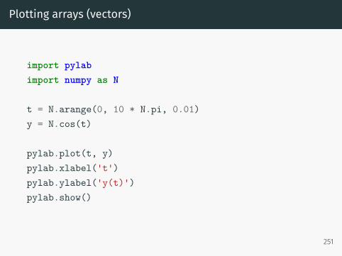
Plotting arrays (vectors)

import pylabimport numpy as N

t = N.arange(0, 10 * N.pi, 0.01)y = N.cos(t)

pylab.plot(t, y)pylab.xlabel('t')pylab.ylabel('y(t)')pylab.show()

251

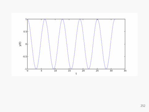
0 5 10 15 20 25 30 35t

-1

-0.5

0

0.5

1y(t

)

252

Matplotlib / Pylab

• Matplotlib tries to make easy things easy and hard thingspossible

• Matplotlib is a 2D plotting library which producespublication quality figures (increasingly also 3d)

• Matplotlib can be fully scripted but interactive interfaceavailable

253

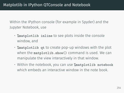
Matplotlib in IPython QTConsole and Notebook

Within the IPython console (for example in Spyder) and theJupyter Notebook, use

• %matplotlib inline to see plots inside the consolewindow, and

• %matplotlib qt to create pop-up windows with the plotwhen the matplotlib.show() command is used. We canmanipulate the view interactively in that window.

• Within the notebook, you can use %matplotlib notebookwhich embeds an interactive window in the note book.

254

Pylab and Matplotlib

PylabPylab is a Matlab-like (state-driven) plotting interface (and comeswith matplotlib).

• Convenient for ’simple’ plots

• Check examples in lecture note text book and

• Make use of help(pylab.plot) to remind you of line styles,symbols etc.

• Check gallery athttp://matplotlib.org/gallery.html#pylab_examples

255

Matplotlib.pyplotMatplotlib.pyplot is an object oriented plotting interface.

• Very fine grained control over plots

• Check gallery at Matplotlib gallery

• Try Matplotlib notebook (on module’s home page) as anintroduction and useful reference.

LAB8

256

Higher Order Functions 2: Functionaltools

More list processing and functional programming

• So far, have processed lists by iterating through themusing for-loop

• perceived to be conceptually simple (by most learners)but

• not as compact as possible and not always as fast aspossible

• Alternatives:• list comprehension• map, filter, reduce, often used with lambda

258

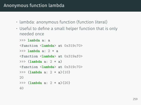
Anonymous function lambda

• lambda: anonymous function (function literal)• Useful to define a small helper function that is onlyneeded once>>> lambda a: a<function <lambda> at 0x319c70>>>> lambda a: 2 * a<function <lambda> at 0x319af0>>>> (lambda a: 2 * a)<function <lambda> at 0x319c70>>>> (lambda a: 2 * a)(10)20>>> (lambda a: 2 * a)(20)40

259

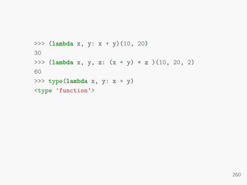
>>> (lambda x, y: x + y)(10, 20)30>>> (lambda x, y, z: (x + y) * z )(10, 20, 2)60>>> type(lambda x, y: x + y)<type 'function'>

260

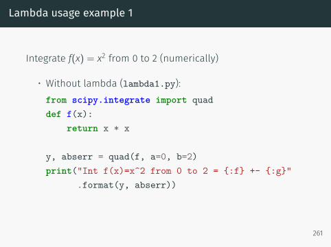
Lambda usage example 1

Integrate f(x) = x2 from 0 to 2 (numerically)

• Without lambda (lambda1.py):from scipy.integrate import quaddef f(x):

return x * x

y, abserr = quad(f, a=0, b=2)print("Int f(x)=x^2 from 0 to 2 = {:f} +- {:g}"

.format(y, abserr))

261

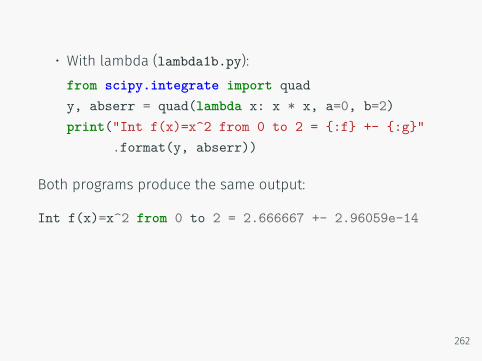
• With lambda (lambda1b.py):from scipy.integrate import quady, abserr = quad(lambda x: x * x, a=0, b=2)print("Int f(x)=x^2 from 0 to 2 = {:f} +- {:g}"

.format(y, abserr))

Both programs produce the same output:

Int f(x)=x^2 from 0 to 2 = 2.666667 +- 2.96059e-14

262

Higher order functions

Roughly: “Functions that take or return functions” (see forexample (Wikipedia entry))

Rough summary (check help(COMMAND) for details)

• map(function, iterable)→ iterable:apply function to all elements in iterable

• filter(function, iterable)→ iterable:return items of iterable for which function(item) is true.

• reduce(function, iterable, initial)→ value:apply function(x,y) from left to right to reduce iterable to asingle value.

Note that sequences are iterables.

263

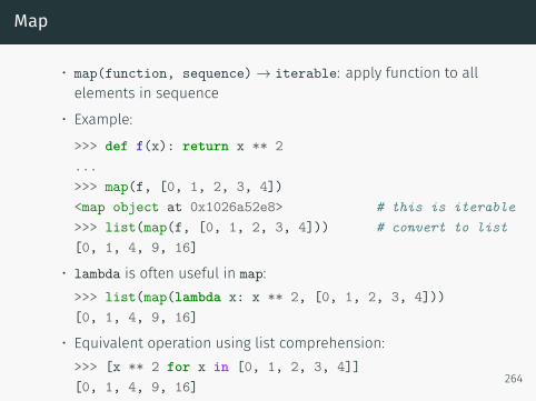
Map

• map(function, sequence)→ iterable: apply function to allelements in sequence

• Example:

>>> def f(x): return x ** 2...>>> map(f, [0, 1, 2, 3, 4])<map object at 0x1026a52e8> # this is iterable>>> list(map(f, [0, 1, 2, 3, 4])) # convert to list[0, 1, 4, 9, 16]

• lambda is often useful in map:>>> list(map(lambda x: x ** 2, [0, 1, 2, 3, 4]))[0, 1, 4, 9, 16]

• Equivalent operation using list comprehension:>>> [x ** 2 for x in [0, 1, 2, 3, 4]][0, 1, 4, 9, 16] 264

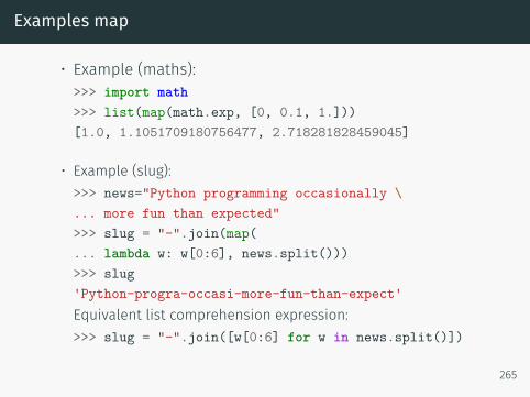
Examples map

• Example (maths):>>> import math>>> list(map(math.exp, [0, 0.1, 1.]))[1.0, 1.1051709180756477, 2.718281828459045]

• Example (slug):>>> news="Python programming occasionally \... more fun than expected">>> slug = "-".join(map(... lambda w: w[0:6], news.split()))>>> slug'Python-progra-occasi-more-fun-than-expect'Equivalent list comprehension expression:>>> slug = "-".join([w[0:6] for w in news.split()])

265

Filter

• filter(function, iterable)→ iterable: return itemsof iterable for which function(item) is true.

• Example:>>> c = "The quick brown fox jumps".split()>>> print(c)['The', 'quick', 'brown', 'fox', 'jumps']>>> def len_gr_4(s):... return len(s) > 4>>> list(map(len_gr_4, c))[False, True, True, False, True]>>> filter(len_gr_4, c)

266

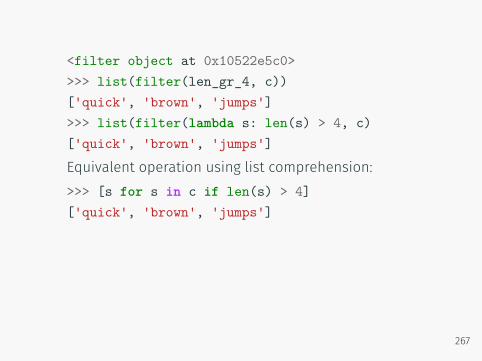
<filter object at 0x10522e5c0>>>> list(filter(len_gr_4, c))['quick', 'brown', 'jumps']>>> list(filter(lambda s: len(s) > 4, c)['quick', 'brown', 'jumps']Equivalent operation using list comprehension:>>> [s for s in c if len(s) > 4]['quick', 'brown', 'jumps']

267

Examples filter

• Example:

>>> def is_positive(n):... return n > 0>>> list(filter(is_positive,... [-3, -2, -1, 0, 1, 2, 3, 4]))[1, 2, 3, 4]>>> list(filter(lambda n:n>0,... [-3, -2, -1, 0, 1, 2, 3, 4]))[1, 2, 3, 4]

List comprehension equivalent:

>>> [x for x in [-3, -2, -1, 0, 1, 2, 3, 4] if x > 0][1, 2, 3, 4]

268

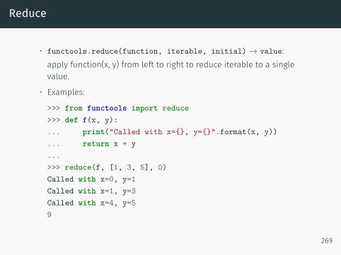
Reduce

• functools.reduce(function, iterable, initial) → value:apply function(x, y) from left to right to reduce iterable to a singlevalue.

• Examples:

>>> from functools import reduce>>> def f(x, y):... print("Called with x={}, y={}".format(x, y))... return x + y...>>> reduce(f, [1, 3, 5], 0)Called with x=0, y=1Called with x=1, y=3Called with x=4, y=59

269

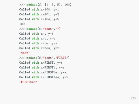
>>> reduce(f, [1, 3, 5], 100)Called with x=100, y=1Called with x=101, y=3Called with x=104, y=5109>>> reduce(f,"test","")Called with x=, y=tCalled with x=t, y=eCalled with x=te, y=sCalled with x=tes, y=t'test'>>> reduce(f,"test","FIRST")Called with x=FIRST, y=tCalled with x=FIRSTt, y=eCalled with x=FIRSTte, y=sCalled with x=FIRSTtes, y=t'FIRSTtest'

270

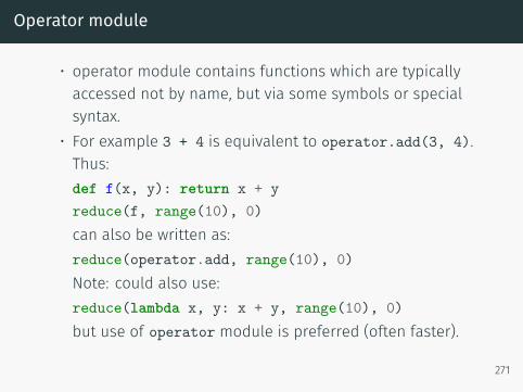
Operator module

• operator module contains functions which are typicallyaccessed not by name, but via some symbols or specialsyntax.

• For example 3 + 4 is equivalent to operator.add(3, 4).Thus:def f(x, y): return x + yreduce(f, range(10), 0)can also be written as:reduce(operator.add, range(10), 0)Note: could also use:reduce(lambda x, y: x + y, range(10), 0)but use of operator module is preferred (often faster).

271

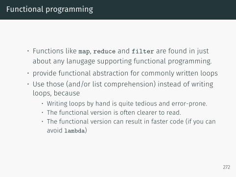
Functional programming

• Functions like map, reduce and filter are found in justabout any lanugage supporting functional programming.

• provide functional abstraction for commonly written loops• Use those (and/or list comprehension) instead of writingloops, because

• Writing loops by hand is quite tedious and error-prone.• The functional version is often clearer to read.• The functional version can result in faster code (if you canavoid lambda)

272

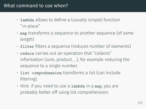
What command to use when?

• lambda allows to define a (usually simple) function”in-place”

• map transforms a sequence to another sequence (of samelength)

• filter filters a sequence (reduces number of elements)• reduce carries out an operation that ”collects”information (sum, product, ...), for example reducing thesequence to a single number.

• list comprehension transforms a list (can includefiltering).

• Hint: if you need to use a lambda in a map, you areprobably better off using list comprehension.

273

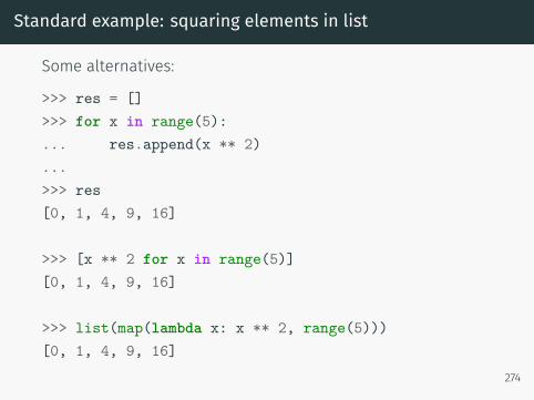
Standard example: squaring elements in list

Some alternatives:

>>> res = []>>> for x in range(5):... res.append(x ** 2)...>>> res[0, 1, 4, 9, 16]

>>> [x ** 2 for x in range(5)][0, 1, 4, 9, 16]

>>> list(map(lambda x: x ** 2, range(5)))[0, 1, 4, 9, 16]

274

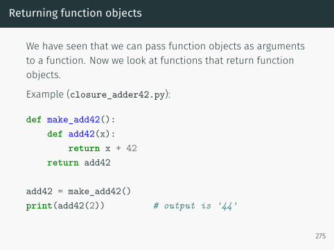
Returning function objects

We have seen that we can pass function objects as argumentsto a function. Now we look at functions that return functionobjects.

Example (closure_adder42.py):

def make_add42():def add42(x):

return x + 42return add42

add42 = make_add42()print(add42(2)) # output is '44'

275

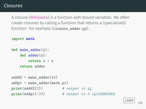
Closures

A closure (Wikipedia) is a function with bound variables. We oftencreate closures by calling a function that returns a (specialised)function. For example (closure_adder.py):

import math

def make_adder(y):def adder(x):

return x + yreturn adder

add42 = make_adder(42)addpi = make_adder(math.pi)print(add42(2)) # output is 44print(addpi(-3)) # output is 0.14159265359

LAB9 276

276

Object Orientation and all that

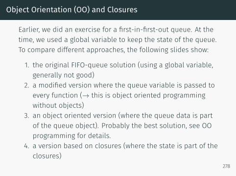
Object Orientation (OO) and Closures

Earlier, we did an exercise for a first-in-first-out queue. At thetime, we used a global variable to keep the state of the queue.To compare different approaches, the following slides show:

1. the original FIFO-queue solution (using a global variable,generally not good)

2. a modified version where the queue variable is passed toevery function (→ this is object oriented programmingwithout objects)

3. an object oriented version (where the queue data is partof the queue object). Probably the best solution, see OOprogramming for details.

4. a version based on closures (where the state is part of theclosures)

278

Original FIFO solution (fifoqueue.py)

queue = []def length():

"""Returns number of waiting customers"""return len(queue)

def show():"""print list of customers, longest waiting customer at end."""for name in queue:

print("waiting customer: {}".format(name))

def add(name):"""Customer with name 'name' joining the queue"""queue.insert(0, name)

def next():"""Returns name of next to serve, removes customer from queue"""return queue.pop()

add('Spearing'); add('Fangohr'); add('Takeda')show(); next() 279

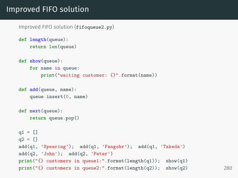
Improved FIFO solution

Improved FIFO solution (fifoqueue2.py)

def length(queue):return len(queue)

def show(queue):for name in queue:

print("waiting customer: {}".format(name))

def add(queue, name):queue.insert(0, name)

def next(queue):return queue.pop()

q1 = []q2 = []add(q1, 'Spearing'); add(q1, 'Fangohr'); add(q1, 'Takeda')add(q2, 'John'); add(q2, 'Peter')print("{} customers in queue1:".format(length(q1)); show(q1)print("{} customers in queue2:".format(length(q2)); show(q2) 280

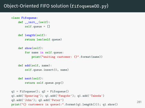
Object-Oriented FIFO solution (fifoqueueOO.py)

class Fifoqueue:def __init__(self):

self.queue = []

def length(self):return len(self.queue)

def show(self):for name in self.queue:

print("waiting customer: {}".format(name))

def add(self, name):self.queue.insert(0, name)

def next(self):return self.queue.pop()

q1 = Fifoqueue(); q2 = Fifoqueue()q1.add('Spearing'); q1.add('Fangohr'); q1.add('Takeda')q2.add('John'); q2.add('Peter')print("{} customers in queue1:".format(q1.length())); q1.show()

281

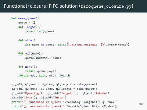
Functional (closure) FIFO solution (fifoqueue_closure.py)

def make_queue():queue = []def length():

return len(queue)

def show():for name in queue: print("waiting customer: {}".format(name))

def add(name):queue.insert(0, name)

def next():return queue.pop()

return add, next, show, length

q1_add, q1_next, q1_show, q1_length = make_queue()q2_add, q2_next, q2_show, q2_length = make_queue()q1_add('Spearing'); q1_add('Fangohr'); q1_add('Takeda')q2_add('John'); q2_add('Peter')print("{} customers in queue1:".format(q1_length()); q1_show()print("{} customers in queue2:".format(q2_length()); q2_show()

282

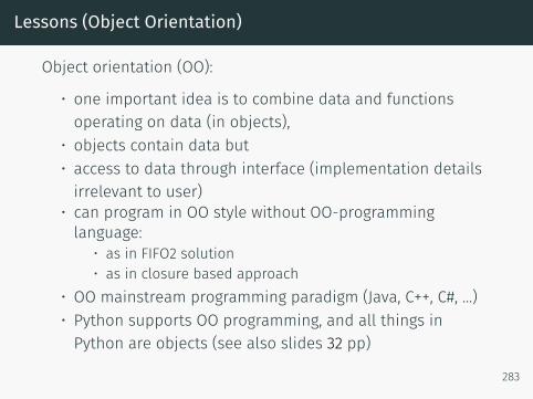
Lessons (Object Orientation)

Object orientation (OO):

• one important idea is to combine data and functionsoperating on data (in objects),

• objects contain data but• access to data through interface (implementation detailsirrelevant to user)

• can program in OO style without OO-programminglanguage:

• as in FIFO2 solution• as in closure based approach

• OO mainstream programming paradigm (Java, C++, C#, ...)• Python supports OO programming, and all things inPython are objects (see also slides 32 pp)

283

283

Numerical Integration

Numerical Integration 1— Overview

Different situations where we use integration:

(A) solving (definite) integrals(B) solving (ordinary) differential equations

• more complicated than (A)• Euler’s method, Runge-Kutta methods

Both (A) and (B) are important.

We begin with the numeric computation of integrals (A).

285

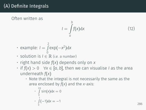
(A) Definite Integrals

Often written as

I =b∫a

f(x)dx (12)

• example: I =2∫0exp(−x2)dx

• solution is I ∈ R (i.e. a number)• right hand side f(x) depends only on x• if f(x) > 0 ∀x ∈ [a,b], then we can visualise I as the areaunderneath f(x)

• Note that the integral is not necessarily the same as thearea enclosed by f(x) and the x-axis:

•2π∫0sin(x)dx = 0

•1∫0(−1)dx = −1

286

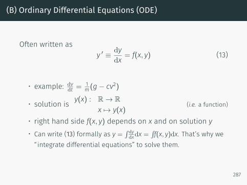
(B) Ordinary Differential Equations (ODE)

Often written asy ′ ≡ dy

dx = f(x, y) (13)

• example: dvdt =

1m(g− cv

2)

• solution is y(x) : R→ Rx 7→ y(x)

(i.e. a function)

• right hand side f(x, y) depends on x and on solution y• Can write (13) formally as y =

∫ dydxdx =

∫f(x, y)dx. That’s why we

“integrate differential equations” to solve them.

287

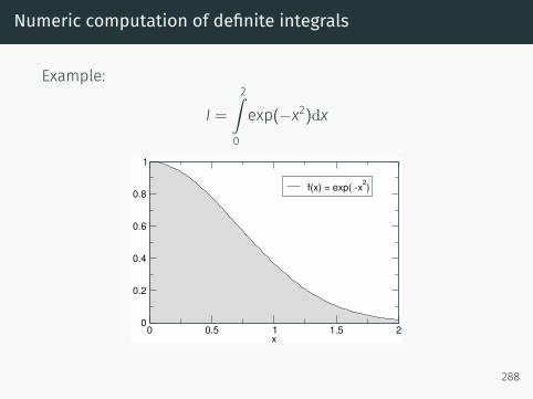
Numeric computation of definite integrals

Example:

I =2∫0

exp(−x2)dx

0 0.5 1 1.5 2x

0

0.2

0.4

0.6

0.8

1

f(x) = exp( -x2)

288

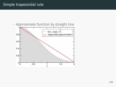
Simple trapezoidal rule

• Approximate function by straight line

0 0.5 1 1.5 2x

0

0.2

0.4

0.6

0.8

1

f(x) = exp( -x2)trapezoidal approximation

289

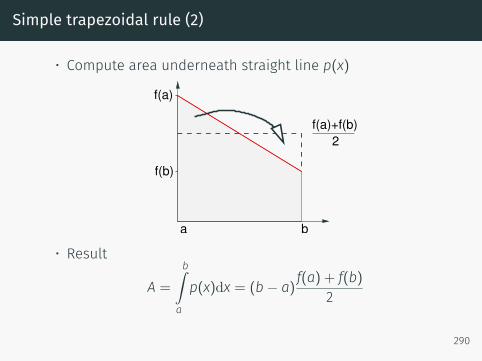
Simple trapezoidal rule (2)

• Compute area underneath straight line p(x)

f(a)+f(b) 2

ba

f(b)

f(a)

• Result

A =

b∫a

p(x)dx = (b− a) f(a) + f(b)2

290

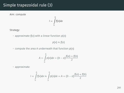
Simple trapezoidal rule (3)

Aim: compute

I =b∫a

f(x)dx

Strategy:

• approximate f(x) with a linear function p(x):

p(x) ≈ f(x)

• compute the area A underneath that function p(x):

A =

b∫a

p(x)dx = (b− a) f(a) + f(b)2

• approximate

I =b∫a

f(x)dx ≈b∫a

p(x)dx = A = (b− a) f(a) + f(b)2

291

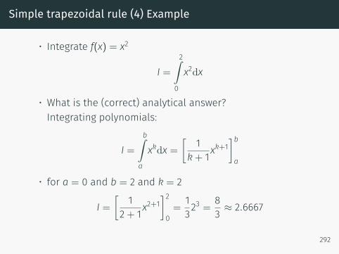
Simple trapezoidal rule (4) Example

• Integrate f(x) = x2

I =2∫0

x2dx

• What is the (correct) analytical answer?Integrating polynomials:

I =b∫a

xkdx =[

1k+ 1x

k+1]ba

• for a = 0 and b = 2 and k = 2

I =[

12+ 1x

2+1]20=132

3 =83 ≈ 2.6667

292

• Using the trapezoidal rule

A = (b− a) f(a) + f(b)2 = 20+ 4

2 = 4

• The correct answer is I = 8/3 and the approximation is A = 4.We thus overestimate I by A−I

I ≈ 50%.• Plotting f(x) = x2 together with the approximation reveals why weoverestimate I

0 0.5 1 1.5 2x

0

1

2

3

4f(x) = x^2trapezoidal approximation p(x)

• The linear approximation, p(x), overestimates f(x) everywhere (exceptat x = a and x = b).Therefore, the integral of p(x) is greater than the integral of f(x).(More formally: f(x) is convex on [a, b] ⇐⇒ f′′(x) ≥ 0 ∀x ∈ [a, b].)

293

Composite trapezoidal rule

Example f(x) = exp(−x2):

I =2∫0

f(x)dx =2∫0

exp(−x2)dx

0 0.5 1 1.5 2x

0

0.2

0.4

0.6

0.8

1

f(x) = exp( -x2)composite trapezoidalapproximation (n=4)

I =0.5∫0

f(x)dx+1∫

0.5

f(x)dx+1.5∫1

f(x)dx+2∫

1.5

f(x)dx

294

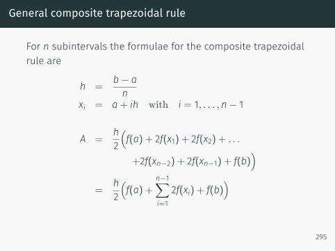
General composite trapezoidal rule

For n subintervals the formulae for the composite trapezoidalrule are

h =b− an

xi = a+ ih with i = 1, . . . ,n− 1

A =h2

(f(a) + 2f(x1) + 2f(x2) + . . .

+2f(xn−2) + 2f(xn−1) + f(b))

=h2

(f(a) +

n−1∑i=1

2f(xi) + f(b))

295

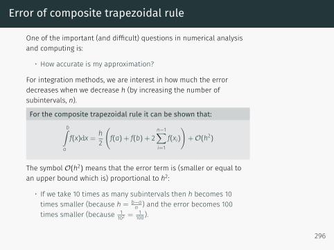
Error of composite trapezoidal rule

One of the important (and difficult) questions in numerical analysisand computing is:

• How accurate is my approximation?

For integration methods, we are interest in how much the errordecreases when we decrease h (by increasing the number ofsubintervals, n).

For the composite trapezoidal rule it can be shown that:b∫a

f(x)dx = h2

(f(a) + f(b) + 2

n−1∑i=1

f(xi))

+O(h2)

The symbol O(h2) means that the error term is (smaller or equal toan upper bound which is) proportional to h2:

• If we take 10 times as many subintervals then h becomes 10times smaller (because h = b−a

n ) and the error becomes 100times smaller (because 1

102 =1100 ).

296

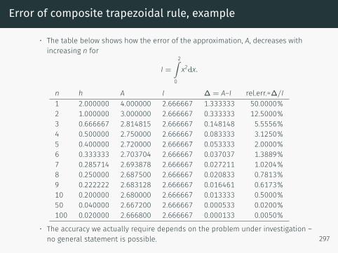
Error of composite trapezoidal rule, example

• The table below shows how the error of the approximation, A, decreases withincreasing n for

I =2∫0

x2dx.

n h A I ∆ = A–I rel.err.=∆/I1 2.000000 4.000000 2.666667 1.333333 50.0000%2 1.000000 3.000000 2.666667 0.333333 12.5000%3 0.666667 2.814815 2.666667 0.148148 5.5556%4 0.500000 2.750000 2.666667 0.083333 3.1250%5 0.400000 2.720000 2.666667 0.053333 2.0000%6 0.333333 2.703704 2.666667 0.037037 1.3889%7 0.285714 2.693878 2.666667 0.027211 1.0204%8 0.250000 2.687500 2.666667 0.020833 0.7813%9 0.222222 2.683128 2.666667 0.016461 0.6173%10 0.200000 2.680000 2.666667 0.013333 0.5000%50 0.040000 2.667200 2.666667 0.000533 0.0200%100 0.020000 2.666800 2.666667 0.000133 0.0050%

• The accuracy we actually require depends on the problem under investigation –no general statement is possible. 297

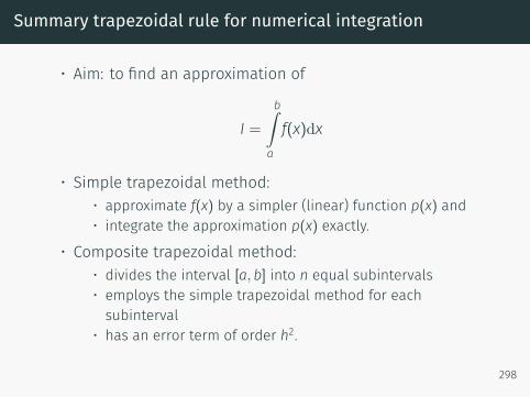
Summary trapezoidal rule for numerical integration

• Aim: to find an approximation of

I =b∫a

f(x)dx

• Simple trapezoidal method:• approximate f(x) by a simpler (linear) function p(x) and• integrate the approximation p(x) exactly.

• Composite trapezoidal method:• divides the interval [a,b] into n equal subintervals• employs the simple trapezoidal method for eachsubinterval

• has an error term of order h2.

298

298

Numpy usage examples

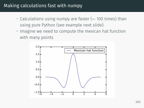
Making calculations fast with numpy

• Calculations using numpy are faster (∼ 100 times) thanusing pure Python (see example next slide).

• Imagine we need to compute the mexican hat functionwith many points

6 4 2 0 2 4 61.0

0.5

0.0

0.5

1.0

1.5

2.0

Mexican hat function

300

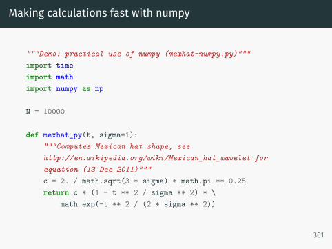
Making calculations fast with numpy

"""Demo: practical use of numpy (mexhat-numpy.py)"""import timeimport mathimport numpy as np

N = 10000

def mexhat_py(t, sigma=1):"""Computes Mexican hat shape, seehttp://en.wikipedia.org/wiki/Mexican_hat_wavelet forequation (13 Dec 2011)"""c = 2. / math.sqrt(3 * sigma) * math.pi ** 0.25return c * (1 - t ** 2 / sigma ** 2) * \

math.exp(-t ** 2 / (2 * sigma ** 2))

301

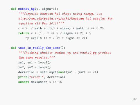
def mexhat_np(t, sigma=1):"""Computes Mexican hat shape using numpy, seehttp://en.wikipedia.org/wiki/Mexican_hat_wavelet forequation (13 Dec 2011)"""c = 2. / math.sqrt(3 * sigma) * math.pi ** 0.25return c * (1 - t ** 2 / sigma ** 2) * \

np.exp(-t ** 2 / (2 * sigma ** 2))

def test_is_really_the_same():"""Checking whether mexhat_np and mexhat_py producethe same results."""xs1, ys1 = loop1()xs2, ys2 = loop2()deviation = math.sqrt(sum((ys1 - ys2) ** 2))print("error:", deviation)assert deviation < 1e-15

302

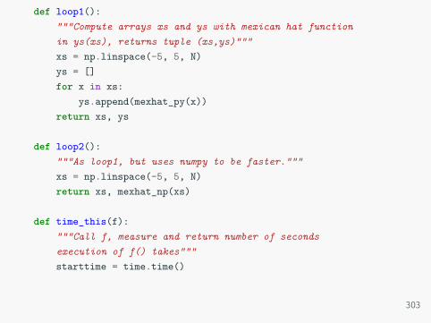
def loop1():"""Compute arrays xs and ys with mexican hat functionin ys(xs), returns tuple (xs,ys)"""xs = np.linspace(-5, 5, N)ys = []for x in xs:

ys.append(mexhat_py(x))return xs, ys

def loop2():"""As loop1, but uses numpy to be faster."""xs = np.linspace(-5, 5, N)return xs, mexhat_np(xs)

def time_this(f):"""Call f, measure and return number of secondsexecution of f() takes"""starttime = time.time()

303

f()stoptime = time.time()return stoptime - starttime

def make_plot(filenameroot):import pylabpylab.figure(figsize=(6, 4))xs, ys = loop2()pylab.plot(xs, ys, label='Mexican hat function')pylab.legend()pylab.savefig(filenameroot + '.png')pylab.savefig(filenameroot + '.pdf')

def main():test_is_really_the_same()make_plot('mexhat1d')time1 = time_this(loop1)time2 = time_this(loop2)

304

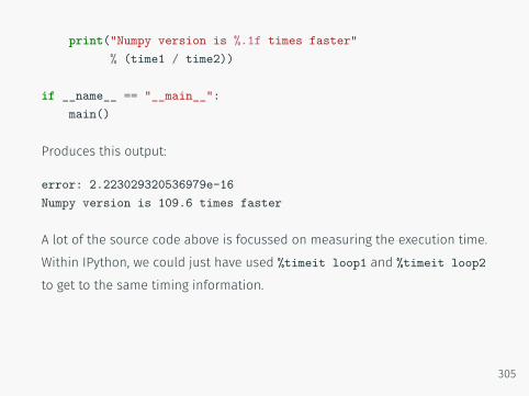
print("Numpy version is %.1f times faster"% (time1 / time2))

if __name__ == "__main__":main()

Produces this output:

error: 2.223029320536979e-16Numpy version is 109.6 times faster

A lot of the source code above is focussed on measuring the execution time.Within IPython, we could just have used %timeit loop1 and %timeit loop2

to get to the same timing information.

305

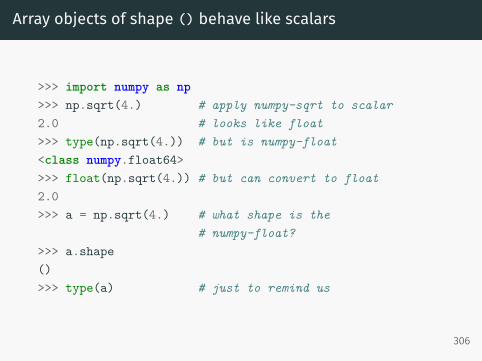
Array objects of shape () behave like scalars

>>> import numpy as np>>> np.sqrt(4.) # apply numpy-sqrt to scalar2.0 # looks like float>>> type(np.sqrt(4.)) # but is numpy-float<class numpy.float64>>>> float(np.sqrt(4.)) # but can convert to float2.0>>> a = np.sqrt(4.) # what shape is the

# numpy-float?>>> a.shape()>>> type(a) # just to remind us

306

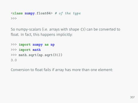
<class numpy.float64> # of the type>>>

So numpy-scalars (i.e. arrays with shape ()) can be converted tofloat. In fact, this happens implicitly:

>>> import numpy as np>>> import math>>> math.sqrt(np.sqrt(81))3.0

Conversion to float fails if array has more than one element:

307

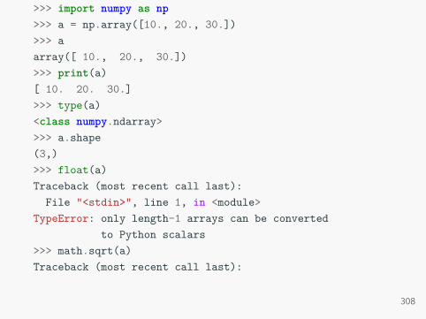
>>> import numpy as np>>> a = np.array([10., 20., 30.])>>> aarray([ 10., 20., 30.])>>> print(a)[ 10. 20. 30.]>>> type(a)<class numpy.ndarray>>>> a.shape(3,)>>> float(a)Traceback (most recent call last):File "<stdin>", line 1, in <module>

TypeError: only length-1 arrays can be convertedto Python scalars

>>> math.sqrt(a)Traceback (most recent call last):

308

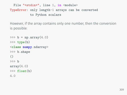
File "<stdin>", line 1, in <module>TypeError: only length-1 arrays can be converted

to Python scalars

However, if the array contains only one number, then the conversionis possible:

>>> b = np.array(4.0)>>> type(b)<class numpy.ndarray>>>> b.shape()>>> barray(4.0)>>> float(b)4.0

309

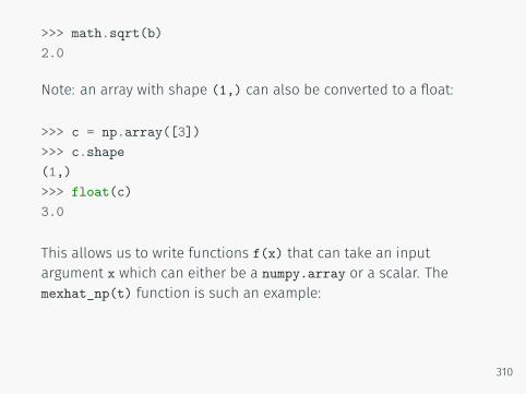
>>> math.sqrt(b)2.0

Note: an array with shape (1,) can also be converted to a float:

>>> c = np.array([3])>>> c.shape(1,)>>> float(c)3.0

This allows us to write functions f(x) that can take an inputargument x which can either be a numpy.array or a scalar. Themexhat_np(t) function is such an example:

310

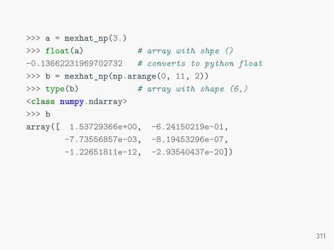
>>> a = mexhat_np(3.)>>> float(a) # array with shpe ()-0.13662231969702732 # converts to python float>>> b = mexhat_np(np.arange(0, 11, 2))>>> type(b) # array with shape (6,)<class numpy.ndarray>>>> barray([ 1.53729366e+00, -6.24150219e-01,

-7.73556857e-03, -8.19453296e-07,-1.22651811e-12, -2.93540437e-20])

311

311

Scientific Python

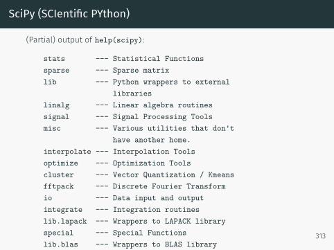
SciPy (SCIentific PYthon)

(Partial) output of help(scipy):

stats --- Statistical Functionssparse --- Sparse matrixlib --- Python wrappers to external

librarieslinalg --- Linear algebra routinessignal --- Signal Processing Toolsmisc --- Various utilities that don't

have another home.interpolate --- Interpolation Toolsoptimize --- Optimization Toolscluster --- Vector Quantization / Kmeansfftpack --- Discrete Fourier Transformio --- Data input and outputintegrate --- Integration routineslib.lapack --- Wrappers to LAPACK libraryspecial --- Special Functionslib.blas --- Wrappers to BLAS library

313

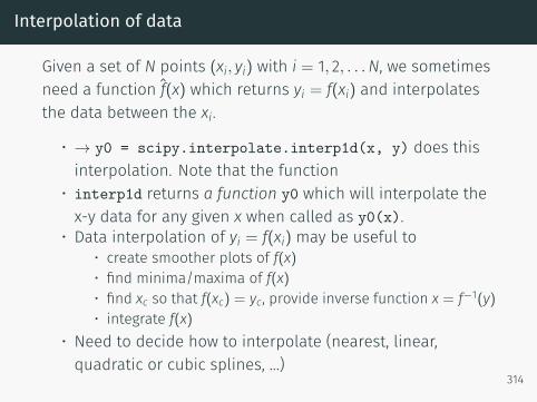
Interpolation of data

Given a set of N points (xi, yi) with i = 1, 2, . . .N, we sometimesneed a function f̂(x) which returns yi = f(xi) and interpolatesthe data between the xi.

• → y0 = scipy.interpolate.interp1d(x, y) does thisinterpolation. Note that the function

• interp1d returns a function y0 which will interpolate thex-y data for any given x when called as y0(x).

• Data interpolation of yi = f(xi) may be useful to• create smoother plots of f(x)• find minima/maxima of f(x)• find xc so that f(xc) = yc, provide inverse function x = f−1(y)• integrate f(x)

• Need to decide how to interpolate (nearest, linear,quadratic or cubic splines, ...)

314

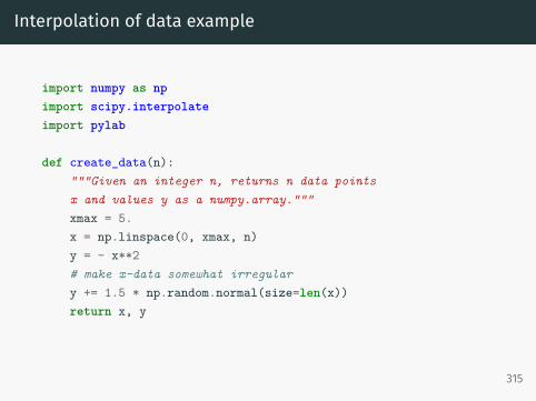
Interpolation of data example

import numpy as npimport scipy.interpolateimport pylab

def create_data(n):"""Given an integer n, returns n data pointsx and values y as a numpy.array."""xmax = 5.x = np.linspace(0, xmax, n)y = - x**2# make x-data somewhat irregulary += 1.5 * np.random.normal(size=len(x))return x, y

315

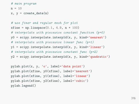
# main programn = 10x, y = create_data(n)

# use finer and regular mesh for plotxfine = np.linspace(0.1, 4.9, n * 100)# interpolate with piecewise constant function (p=0)y0 = scipy.interpolate.interp1d(x, y, kind='nearest')# interpolate with piecewise linear func (p=1)y1 = scipy.interpolate.interp1d(x, y, kind='linear')# interpolate with piecewise constant func (p=2)y2 = scipy.interpolate.interp1d(x, y, kind='quadratic')

pylab.plot(x, y, 'o', label='data point')pylab.plot(xfine, y0(xfine), label='nearest')pylab.plot(xfine, y1(xfine), label='linear')pylab.plot(xfine, y2(xfine), label='cubic')pylab.legend()

316

pylab.xlabel('x')pylab.savefig('interpolate.pdf')pylab.show()

317

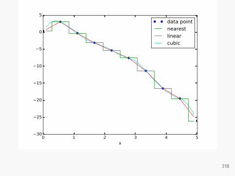
0 1 2 3 4 5x

30

25

20

15

10

5

0

5

data pointnearestlinearcubic

318

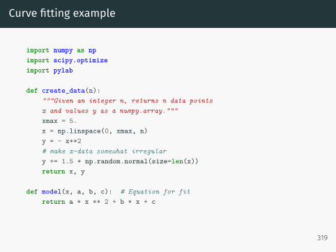
Curve fitting example

import numpy as npimport scipy.optimizeimport pylab

def create_data(n):"""Given an integer n, returns n data pointsx and values y as a numpy.array."""xmax = 5.x = np.linspace(0, xmax, n)y = - x**2# make x-data somewhat irregulary += 1.5 * np.random.normal(size=len(x))return x, y

def model(x, a, b, c): # Equation for fitreturn a * x ** 2 + b * x + c

319

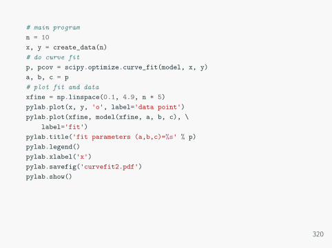
# main programn = 10x, y = create_data(n)# do curve fitp, pcov = scipy.optimize.curve_fit(model, x, y)a, b, c = p# plot fit and dataxfine = np.linspace(0.1, 4.9, n * 5)pylab.plot(x, y, 'o', label='data point')pylab.plot(xfine, model(xfine, a, b, c), \

label='fit')pylab.title('fit parameters (a,b,c)=%s' % p)pylab.legend()pylab.xlabel('x')pylab.savefig('curvefit2.pdf')pylab.show()

320

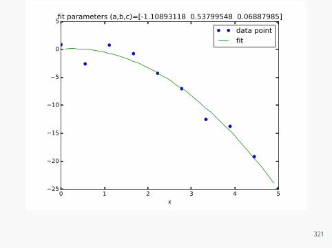
0 1 2 3 4 5x

25

20

15

10

5

0

5fit parameters (a,b,c)=[-1.10893118 0.53799548 0.06887985]

data pointfit

321

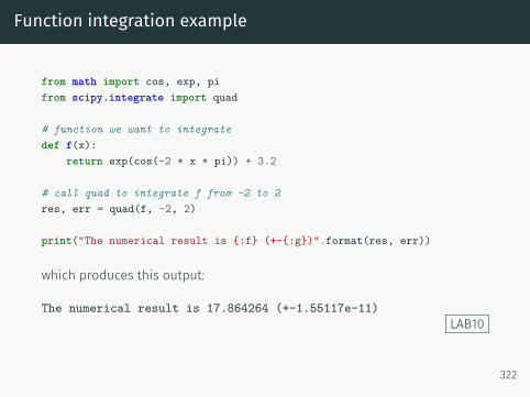
Function integration example

from math import cos, exp, pifrom scipy.integrate import quad

# function we want to integratedef f(x):

return exp(cos(-2 * x * pi)) + 3.2

# call quad to integrate f from -2 to 2res, err = quad(f, -2, 2)

print("The numerical result is {:f} (+-{:g})".format(res, err))

which produces this output:

The numerical result is 17.864264 (+-1.55117e-11)LAB10

322

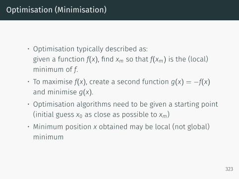
Optimisation (Minimisation)

• Optimisation typically described as:given a function f(x), find xm so that f(xm) is the (local)minimum of f.

• To maximise f(x), create a second function g(x) = −f(x)and minimise g(x).

• Optimisation algorithms need to be given a starting point(initial guess x0 as close as possible to xm)

• Minimum position x obtained may be local (not global)minimum

323

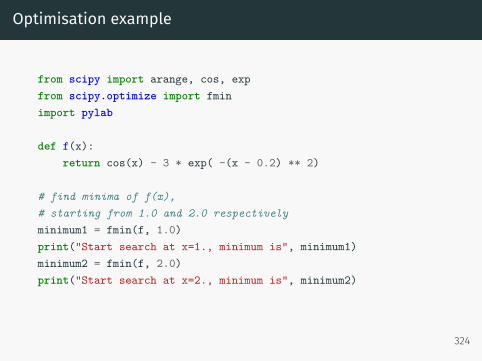
Optimisation example

from scipy import arange, cos, expfrom scipy.optimize import fminimport pylab

def f(x):return cos(x) - 3 * exp( -(x - 0.2) ** 2)

# find minima of f(x),# starting from 1.0 and 2.0 respectivelyminimum1 = fmin(f, 1.0)print("Start search at x=1., minimum is", minimum1)minimum2 = fmin(f, 2.0)print("Start search at x=2., minimum is", minimum2)

324

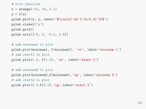
# plot functionx = arange(-10, 10, 0.1)y = f(x)pylab.plot(x, y, label='$\cos(x)-3e^{-(x-0.2)^2}$')pylab.xlabel('x')pylab.grid()pylab.axis([-5, 5, -2.2, 0.5])

# add minimum1 to plotpylab.plot(minimum1, f(minimum1), 'vr', label='minimum 1')# add start1 to plotpylab.plot(1.0, f(1.0), 'or', label='start 1')

# add minimum2 to plotpylab.plot(minimum2,f(minimum2),'vg', label='minimum 2')# add start2 to plotpylab.plot(2.0,f(2.0),'og',label='start 2')

325

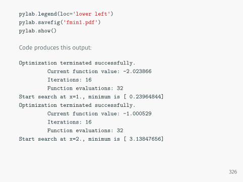
pylab.legend(loc='lower left')pylab.savefig('fmin1.pdf')pylab.show()

Code produces this output:

Optimization terminated successfully.Current function value: -2.023866Iterations: 16Function evaluations: 32

Start search at x=1., minimum is [ 0.23964844]Optimization terminated successfully.

Current function value: -1.000529Iterations: 16Function evaluations: 32

Start search at x=2., minimum is [ 3.13847656]

326

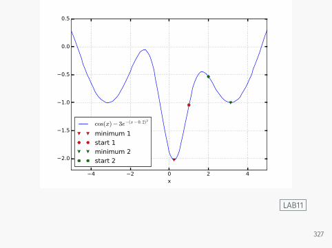
4 2 0 2 4x

2.0

1.5

1.0

0.5

0.0

0.5

cos(x)− 3e−(x− 0. 2)2

minimum 1start 1minimum 2start 2

LAB11

327

ODEs

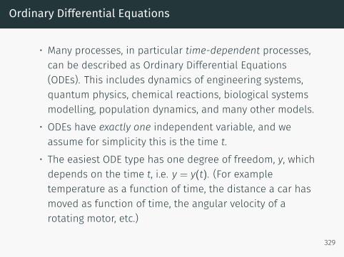
Ordinary Differential Equations

• Many processes, in particular time-dependent processes,can be described as Ordinary Differential Equations(ODEs). This includes dynamics of engineering systems,quantum physics, chemical reactions, biological systemsmodelling, population dynamics, and many other models.

• ODEs have exactly one independent variable, and weassume for simplicity this is the time t.

• The easiest ODE type has one degree of freedom, y, whichdepends on the time t, i.e. y = y(t). (For exampletemperature as a function of time, the distance a car hasmoved as function of time, the angular velocity of arotating motor, etc.)

329

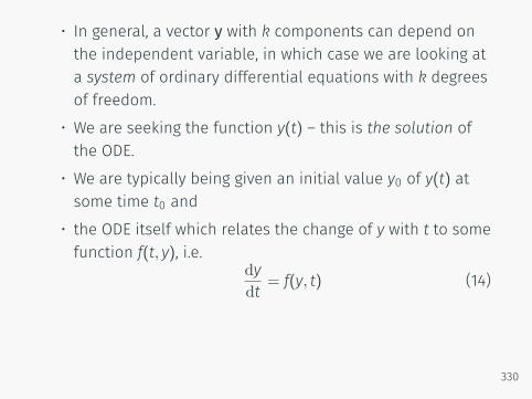
• In general, a vector y with k components can depend onthe independent variable, in which case we are looking ata system of ordinary differential equations with k degreesof freedom.

• We are seeking the function y(t) – this is the solution ofthe ODE.

• We are typically being given an initial value y0 of y(t) atsome time t0 and

• the ODE itself which relates the change of y with t to somefunction f(t, y), i.e.

dydt = f(y, t) (14)

330

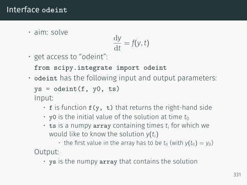
Interface odeint

• aim: solvedydt = f(y, t)

• get access to “odeint”:from scipy.integrate import odeint

• odeint has the following input and output parameters:ys = odeint(f, y0, ts)Input:

• f is function f(y, t) that returns the right-hand side• y0 is the initial value of the solution at time t0• ts is a numpy array containing times ti for which wewould like to know the solution y(ti)

• the first value in the array has to be t0 (with y(t0) = y0)Output:

• ys is the numpy array that contains the solution

331

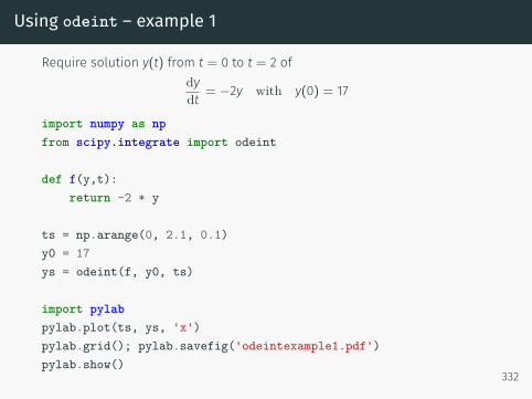
Using odeint – example 1

Require solution y(t) from t = 0 to t = 2 ofdydt = −2y with y(0) = 17

import numpy as npfrom scipy.integrate import odeint

def f(y,t):return -2 * y

ts = np.arange(0, 2.1, 0.1)y0 = 17ys = odeint(f, y0, ts)

import pylabpylab.plot(ts, ys, 'x')pylab.grid(); pylab.savefig('odeintexample1.pdf')pylab.show()

332

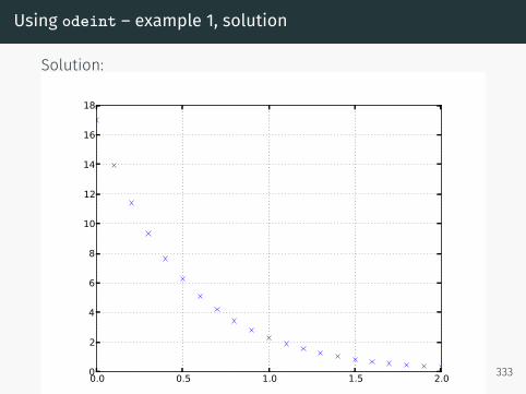
Using odeint – example 1, solution

Solution:

0.0 0.5 1.0 1.5 2.00

2

4

6

8

10

12

14

16

18

333

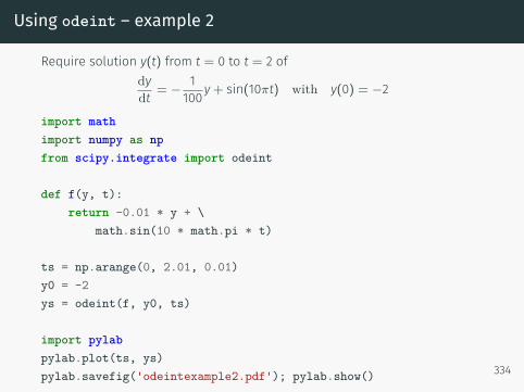
Using odeint – example 2

Require solution y(t) from t = 0 to t = 2 ofdydt = − 1

100y+ sin(10πt) with y(0) = −2

import mathimport numpy as npfrom scipy.integrate import odeint

def f(y, t):return -0.01 * y + \

math.sin(10 * math.pi * t)

ts = np.arange(0, 2.01, 0.01)y0 = -2ys = odeint(f, y0, ts)

import pylabpylab.plot(ts, ys)pylab.savefig('odeintexample2.pdf'); pylab.show() 334

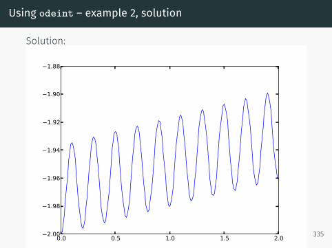
Using odeint – example 2, solution

Solution:

0.0 0.5 1.0 1.5 2.02.00

1.98

1.96

1.94

1.92

1.90

1.88

335

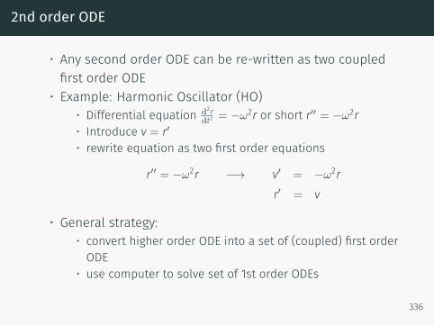
2nd order ODE

• Any second order ODE can be re-written as two coupledfirst order ODE

• Example: Harmonic Oscillator (HO)• Differential equation d2r

dt2 = −ω2r or short r′′ = −ω2r

• Introduce v = r′• rewrite equation as two first order equations

r′′ = −ω2r −→ v′ = −ω2rr′ = v

• General strategy:• convert higher order ODE into a set of (coupled) first orderODE

• use computer to solve set of 1st order ODEs

336

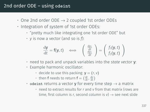
2nd order ODE – using odeint

• One 2nd order ODE→ 2 coupled 1st order ODEs• Integration of system of 1st order ODEs:

• “pretty much like integrating one 1st order ODE” but• y is now a vector (and so is f):

dydt = f(y, t) ⇐⇒

(dy1dtdy2dt

)=

(f1(y, t)f2(y, t)

)• need to pack and unpack variables into the state vector y:• Example harmonic oscillator:

• decide to use this packing: y = (r, v)• then f needs to return f =

(drdt ,

dvdt)

• odeint returns a vector y for every time step→ a matrix• need to extract results for r and v from that matrix (rows aretime, first column is r, second column is v)→ see next slide

337

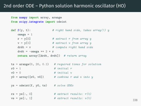
2nd order ODE – Python solution harmonic oscillator (HO)

from numpy import array, arangefrom scipy.integrate import odeint

def f(y, t): # right hand side, takes array(!) yomega = 1r = y[0] # extract r from array yv = y[1] # extract v from array ydrdt = v # compute right hand sidedvdt = -omega ** 2 * rreturn array([drdt, dvdt]) # return array

ts = arange(0, 20, 0.1) # required times for solutionr0 = 1 # initial rv0 = 0 # initial vy0 = array([r0, v0]) # combine r and v into y

ys = odeint(f, y0, ts) # solve ODEs

rs = ys[:, 0] # extract results: r(t)vs = ys[:, 1] # extract results: v(t) 338

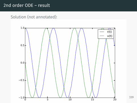
2nd order ODE – result

Solution (not annotated):

0 5 10 15 201.0

0.5

0.0

0.5

1.0

r(t)v(t)

339

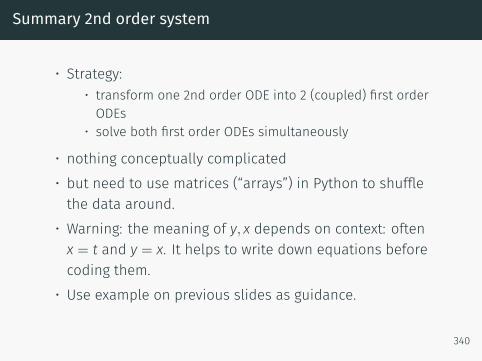
Summary 2nd order system

• Strategy:• transform one 2nd order ODE into 2 (coupled) first orderODEs

• solve both first order ODEs simultaneously

• nothing conceptually complicated• but need to use matrices (“arrays”) in Python to shufflethe data around.

• Warning: the meaning of y, x depends on context: oftenx = t and y = x. It helps to write down equations beforecoding them.

• Use example on previous slides as guidance.

340

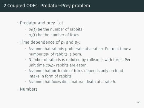
2 Coupled ODEs: Predator-Prey problem

• Predator and prey. Let• p1(t) be the number of rabbits• p2(t) be the number of foxes

• Time dependence of p1 and p2:• Assume that rabbits proliferate at a rate a. Per unit time anumber ap1 of rabbits is born.

• Number of rabbits is reduced by collisions with foxes. Perunit time cp1p2 rabbits are eaten.

• Assume that birth rate of foxes depends only on foodintake in form of rabbits.

• Assume that foxes die a natural death at a rate b.

• Numbers

341

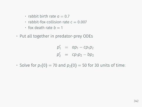
• rabbit birth rate a = 0.7• rabbit-fox-collision rate c = 0.007• fox death rate b = 1

• Put all together in predator-prey ODEs

p′1 = ap1 − cp1p2p′2 = cp1p2 − bp2

• Solve for p1(0) = 70 and p2(0) = 50 for 30 units of time:

342

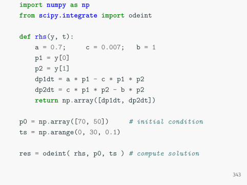
import numpy as npfrom scipy.integrate import odeint

def rhs(y, t):a = 0.7; c = 0.007; b = 1p1 = y[0]p2 = y[1]dp1dt = a * p1 - c * p1 * p2dp2dt = c * p1 * p2 - b * p2return np.array([dp1dt, dp2dt])

p0 = np.array([70, 50]) # initial conditionts = np.arange(0, 30, 0.1)

res = odeint( rhs, p0, ts ) # compute solution

343

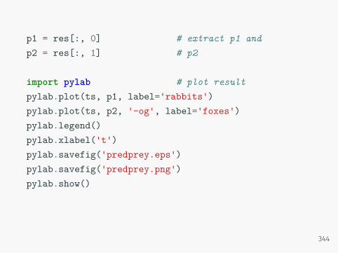
p1 = res[:, 0] # extract p1 andp2 = res[:, 1] # p2

import pylab # plot resultpylab.plot(ts, p1, label='rabbits')pylab.plot(ts, p2, '-og', label='foxes')pylab.legend()pylab.xlabel('t')pylab.savefig('predprey.eps')pylab.savefig('predprey.png')pylab.show()

344

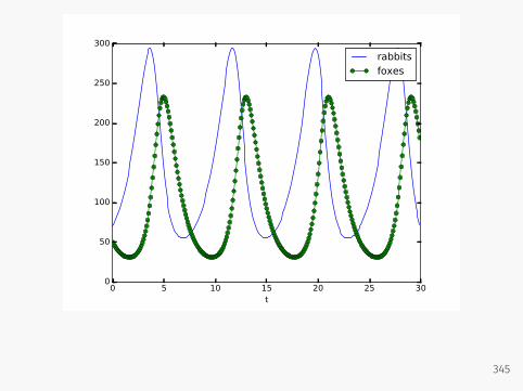
0 5 10 15 20 25 30t

0

50

100

150

200

250

300

rabbitsfoxes

345

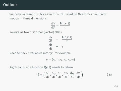
Outlook

Suppose we want to solve a (vector) ODE based on Newton’s equation ofmotion in three dimensions:

d2rdt2 =

F(r, v, t)m

Rewrite as two first order (vector) ODEs:dvdt =

F(r, v, t)m

drdt = v

Need to pack 6 variables into “y”: for example

y = (rx, ry, rz, vx, vy, vz)

Right-hand-side function f(y, t) needs to return:

f =(

drxdt ,

drydt ,

drzdt ,

dvxdt ,

dvydt ,

dvzdt

)(15)

346

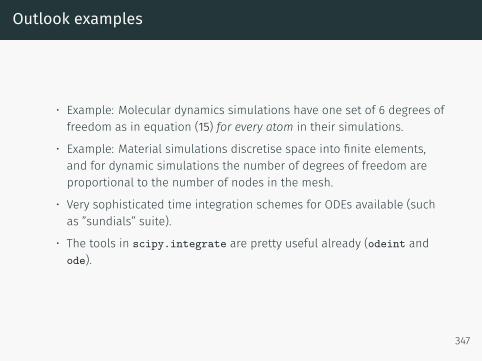
Outlook examples

• Example: Molecular dynamics simulations have one set of 6 degrees offreedom as in equation (15) for every atom in their simulations.

• Example: Material simulations discretise space into finite elements,and for dynamic simulations the number of degrees of freedom areproportional to the number of nodes in the mesh.

• Very sophisticated time integration schemes for ODEs available (suchas ”sundials” suite).

• The tools in scipy.integrate are pretty useful already (odeint andode).

347

Sympy

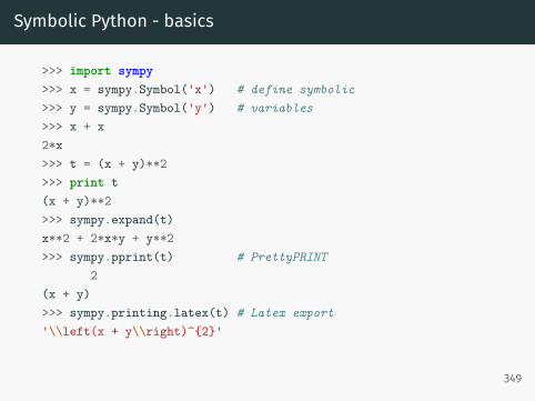
Symbolic Python - basics

>>> import sympy>>> x = sympy.Symbol('x') # define symbolic>>> y = sympy.Symbol('y') # variables>>> x + x2*x>>> t = (x + y)**2>>> print t(x + y)**2>>> sympy.expand(t)x**2 + 2*x*y + y**2>>> sympy.pprint(t) # PrettyPRINT

2(x + y)>>> sympy.printing.latex(t) # Latex export'\\left(x + y\\right)^{2}'

349

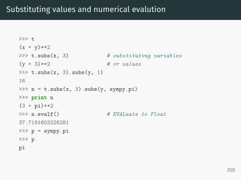
Substituting values and numerical evalution

>>> t(x + y)**2>>> t.subs(x, 3) # substituting variables(y + 3)**2 # or values>>> t.subs(x, 3).subs(y, 1)16>>> n = t.subs(x, 3).subs(y, sympy.pi)>>> print n(3 + pi)**2>>> n.evalf() # EVALuate to Float37.7191603226281>>> p = sympy.pi>>> ppi

350

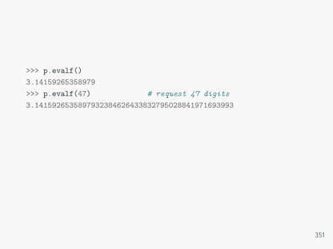
>>> p.evalf()3.14159265358979>>> p.evalf(47) # request 47 digits3.1415926535897932384626433832795028841971693993

351

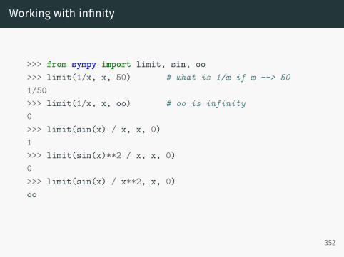
Working with infinity

>>> from sympy import limit, sin, oo>>> limit(1/x, x, 50) # what is 1/x if x --> 501/50>>> limit(1/x, x, oo) # oo is infinity0>>> limit(sin(x) / x, x, 0)1>>> limit(sin(x)**2 / x, x, 0)0>>> limit(sin(x) / x**2, x, 0)oo

352

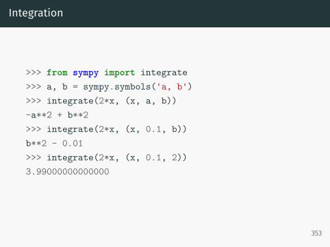
Integration

>>> from sympy import integrate>>> a, b = sympy.symbols('a, b')>>> integrate(2*x, (x, a, b))-a**2 + b**2>>> integrate(2*x, (x, 0.1, b))b**2 - 0.01>>> integrate(2*x, (x, 0.1, 2))3.99000000000000

353

Taylor series

>>> from sympy import series>>> taylorseries = series(sin(x), x, 0)>>> taylorseriesx - x**3/6 + x**5/120 + O(x**6)>>> sympy.pprint(taylorseries)

3 5x x

x - -- + --- + O(x**6)6 120

>>> taylorseries = series(sin(x), x, 0, n=10)>>> sympy.pprint(taylorseries)

3 5 7 9x x x x

x - -- + --- - ---- + ------ + O(x**10)6 120 5040 362880

354

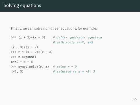
Solving equations

Finally, we can solve non-linear equations, for example:

>>> (x + 2)*(x - 3) # define quadratic equation# with roots x=-2, x=3

(x - 3)*(x + 2)>>> r = (x + 2)*(x - 3)>>> r.expand()x**2 - x - 6>>> sympy.solve(r, x) # solve r = 0[-2, 3] # solution is x = -2, 3

355

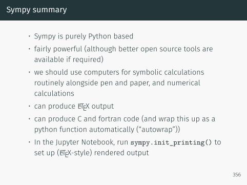
Sympy summary

• Sympy is purely Python based• fairly powerful (although better open source tools areavailable if required)

• we should use computers for symbolic calculationsroutinely alongside pen and paper, and numericalcalculations

• can produce LATEX output• can produce C and fortran code (and wrap this up as apython function automatically (“autowrap”))

• In the Jupyter Notebook, run sympy.init_printing() toset up (LATEX-style) rendered output

356

356

Testing

Testing - context

• Writing code is easy – debugging it is hard• When debugging, we always test code• Later code changes may require repeated testing• Best to automate testing by writing functions that containtests

• A big topic: here we provide some key ideas• We use Python extension tool py.test, see pytest.org

358

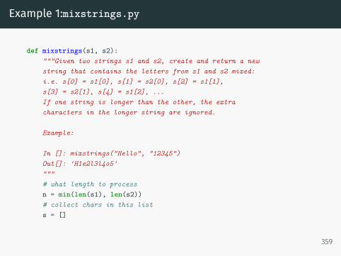
Example 1:mixstrings.py

def mixstrings(s1, s2):"""Given two strings s1 and s2, create and return a newstring that contains the letters from s1 and s2 mixed:i.e. s[0] = s1[0], s[1] = s2[0], s[2] = s1[1],s[3] = s2[1], s[4] = s1[2], ...If one string is longer than the other, the extracharacters in the longer string are ignored.

Example:

In []: mixstrings("Hello", "12345")Out[]: 'H1e2l3l4o5'"""# what length to processn = min(len(s1), len(s2))# collect chars in this lists = []

359

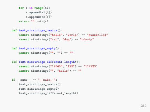
for i in range(n):s.append(s1[i])s.append(s2[i])

return "".join(s)

def test_mixstrings_basics():assert mixstrings("hello", "world") == "hweolrllod"assert mixstrings("cat", "dog") == "cdaotg"

def test_mixstrings_empty():assert mixstrings("", "") == ""

def test_mixstrings_different_length():assert mixstrings("12345", "123") == "112233"assert mixstrings("", "hello") == ""

if __name__ == "__main__":test_mixstrings_basics()test_mixstrings_empty()test_mixstrings_different_length()

360

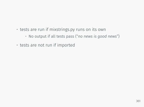
• tests are run if mixstrings.py runs on its own• No output if all tests pass (“no news is good news”)

• tests are not run if imported

361

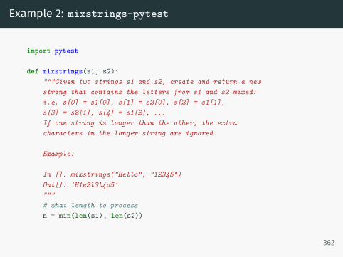
Example 2: mixstrings-pytest

import pytest

def mixstrings(s1, s2):"""Given two strings s1 and s2, create and return a newstring that contains the letters from s1 and s2 mixed:i.e. s[0] = s1[0], s[1] = s2[0], s[2] = s1[1],s[3] = s2[1], s[4] = s1[2], ...If one string is longer than the other, the extracharacters in the longer string are ignored.

Example:

In []: mixstrings("Hello", "12345")Out[]: 'H1e2l3l4o5'"""# what length to processn = min(len(s1), len(s2))

362

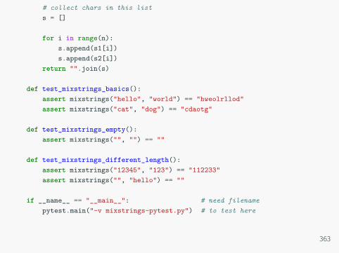
# collect chars in this lists = []

for i in range(n):s.append(s1[i])s.append(s2[i])

return "".join(s)

def test_mixstrings_basics():assert mixstrings("hello", "world") == "hweolrllod"assert mixstrings("cat", "dog") == "cdaotg"

def test_mixstrings_empty():assert mixstrings("", "") == ""

def test_mixstrings_different_length():assert mixstrings("12345", "123") == "112233"assert mixstrings("", "hello") == ""

if __name__ == "__main__": # need filenamepytest.main("-v mixstrings-pytest.py") # to test here

363

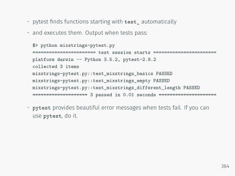
• pytest finds functions starting with test_ automatically

• and executes them. Output when tests pass:

$> python mixstrings-pytest.py======================= test session starts =======================platform darwin -- Python 3.5.2, pytest-2.9.2collected 3 itemsmixstrings-pytest.py::test_mixstrings_basics PASSEDmixstrings-pytest.py::test_mixstrings_empty PASSEDmixstrings-pytest.py::test_mixstrings_different_length PASSED==================== 3 passed in 0.01 seconds =====================

• pytest provides beautiful error messages when tests fail. If you canuse pytest, do it.

364

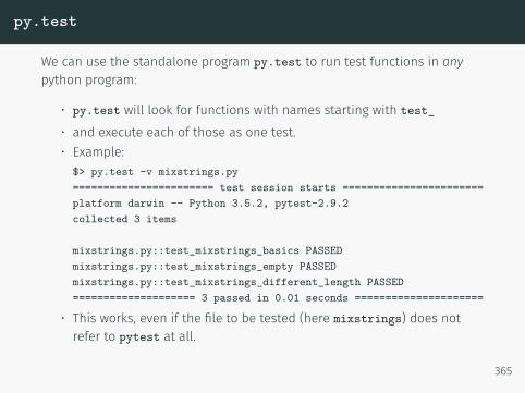
py.test

We can use the standalone program py.test to run test functions in anypython program:

• py.test will look for functions with names starting with test_

• and execute each of those as one test.• Example:$> py.test -v mixstrings.py======================= test session starts =======================platform darwin -- Python 3.5.2, pytest-2.9.2collected 3 items

mixstrings.py::test_mixstrings_basics PASSEDmixstrings.py::test_mixstrings_empty PASSEDmixstrings.py::test_mixstrings_different_length PASSED==================== 3 passed in 0.01 seconds =====================

• This works, even if the file to be tested (here mixstrings) does notrefer to pytest at all.

365

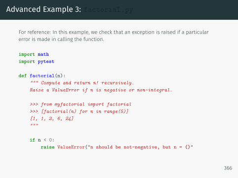
Advanced Example 3: factorial.py

For reference: In this example, we check that an exception is raised if a particularerror is made in calling the function.

import mathimport pytest

def factorial(n):""" Compute and return n! recursively.Raise a ValueError if n is negative or non-integral.

>>> from myfactorial import factorial>>> [factorial(n) for n in range(5)][1, 1, 2, 6, 24]"""

if n < 0:raise ValueError("n should be not-negative, but n = {}"

366

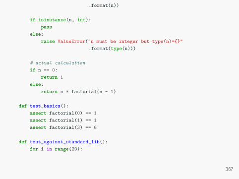
.format(n))

if isinstance(n, int):pass

else:raise ValueError("n must be integer but type(n)={}"

.format(type(n)))

# actual calculationif n == 0:

return 1else:

return n * factorial(n - 1)

def test_basics():assert factorial(0) == 1assert factorial(1) == 1assert factorial(3) == 6

def test_against_standard_lib():for i in range(20):

367

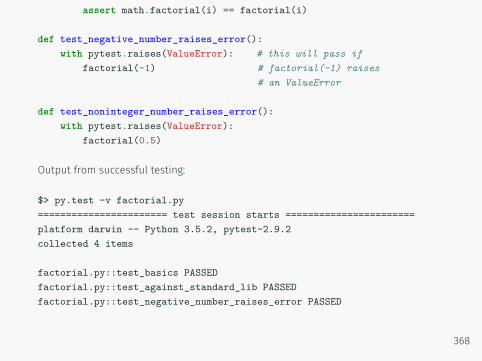
assert math.factorial(i) == factorial(i)

def test_negative_number_raises_error():with pytest.raises(ValueError): # this will pass if

factorial(-1) # factorial(-1) raises# an ValueError

def test_noninteger_number_raises_error():with pytest.raises(ValueError):

factorial(0.5)

Output from successful testing:

$> py.test -v factorial.py======================= test session starts =======================platform darwin -- Python 3.5.2, pytest-2.9.2collected 4 items

factorial.py::test_basics PASSEDfactorial.py::test_against_standard_lib PASSEDfactorial.py::test_negative_number_raises_error PASSED

368

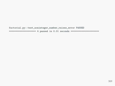
factorial.py::test_noninteger_number_raises_error PASSED==================== 4 passed in 0.01 seconds =====================

369

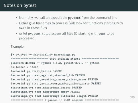
Notes on pytest

• Normally, we call an executable py.test from the command line• Either give filenames to process (will look for functions starting withtest in those files

• or let py.test autodiscover all files (!) starting with test to beprocessed.

Example:

$> py.test -v factorial.py mixstrings.py======================= test session starts =======================platform darwin -- Python 3.5.2, pytest-2.9.2 -- pythoncollected 7 itemsfactorial.py::test_basics PASSEDfactorial.py::test_against_standard_lib PASSEDfactorial.py::test_negative_number_raises_error PASSEDfactorial.py::test_noninteger_number_raises_error PASSEDmixstrings.py::test_mixstrings_basics PASSEDmixstrings.py::test_mixstrings_empty PASSEDmixstrings.py::test_mixstrings_different_length PASSED==================== 7 passed in 0.01 seconds =====================

370

Testing summary

• Unit testing, integration testing, regression testing, systemtesting

• absolute key role in modern software engineering• good practice to always write tests when code is written• bigger projects have ”continuous integration testing”• ”eXtreme Programming” (XP) philosophy suggests to writetests before you write code (”test-driven-development(TDD)”)

• More on this in FEEG6002 Advanced ComputationalMethods

Executable py.test and python module pytest are not part ofthe standard python library.

371

Object Oriented Programming

Overview

• Motivation and terminology• Time example

• encapsulation• defined interfaces to hide data and implementation• operator overloading• inheritance• (teaching example only: normally datetime and others)

• Geometry example• Objects we have used already• Summary

373

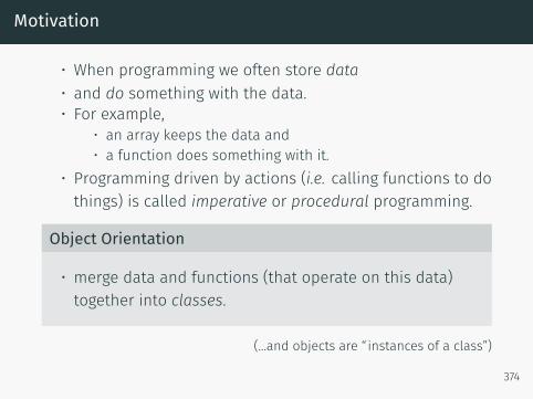
Motivation

• When programming we often store data• and do something with the data.• For example,

• an array keeps the data and• a function does something with it.

• Programming driven by actions (i.e. calling functions to dothings) is called imperative or procedural programming.

Object Orientation

• merge data and functions (that operate on this data)together into classes.

(…and objects are “instances of a class”)

374

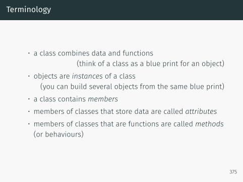
Terminology

• a class combines data and functions(think of a class as a blue print for an object)

• objects are instances of a class(you can build several objects from the same blue print)

• a class contains members• members of classes that store data are called attributes• members of classes that are functions are called methods(or behaviours)

375

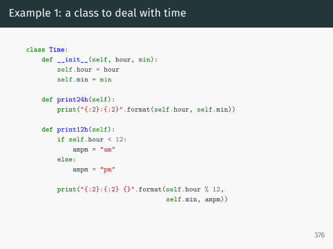
Example 1: a class to deal with time

class Time:def __init__(self, hour, min):

self.hour = hourself.min = min

def print24h(self):print("{:2}:{:2}".format(self.hour, self.min))

def print12h(self):if self.hour < 12:

ampm = "am"else:

ampm = "pm"

print("{:2}:{:2} {}".format(self.hour % 12,self.min, ampm))

376

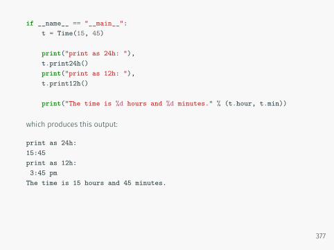
if __name__ == "__main__":t = Time(15, 45)

print("print as 24h: "),t.print24h()print("print as 12h: "),t.print12h()

print("The time is %d hours and %d minutes." % (t.hour, t.min))

which produces this output:

print as 24h:15:45print as 12h:3:45 pmThe time is 15 hours and 45 minutes.

377

• class Time: starts the definition of a class with name Time

• __init__ is the constructor and is called whenever a new object iscreated

• all methods in a class need self as the first argument. Self representsthe object. (This will make more sense later.)

• variables can be stored and are available everywhere within the objectwhen assigned to self, such as self.hour in the example.

• in the main program:

• t = Time(15, 45) creates the object t↔ t is an instance of the class Time

• methods of t can be called like this t.print24h().

This was a mini-example demonstrating how data attributes (i.e. hour andmin) and methods (i.e. print24h() and print12h()) are combined in theTime class.

378

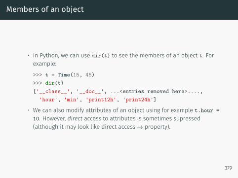
Members of an object

• In Python, we can use dir(t) to see the members of an object t. Forexample:

>>> t = Time(15, 45)>>> dir(t)['__class__', '__doc__', ...<entries removed here>....,

'hour', 'min', 'print12h', 'print24h']

• We can also modify attributes of an object using for example t.hour =10. However, direct access to attributes is sometimes supressed(although it may look like direct access→ property).

379

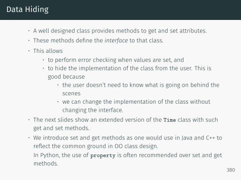
Data Hiding

• A well designed class provides methods to get and set attributes.• These methods define the interface to that class.• This allows

• to perform error checking when values are set, and• to hide the implementation of the class from the user. This isgood because

• the user doesn’t need to know what is going on behind thescenes

• we can change the implementation of the class withoutchanging the interface.

• The next slides show an extended version of the Time class with suchget and set methods.

• We introduce set and get methods as one would use in Java and C++ toreflect the common ground in OO class design.In Python, the use of property is often recommended over set and getmethods.

380

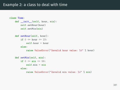
Example 2: a class to deal with time

class Time:def __init__(self, hour, min):

self.setHour(hour)self.setMin(min)

def setHour(self, hour):if 0 <= hour <= 23:

self.hour = hourelse:

raise ValueError("Invalid hour value: %d" % hour)

def setMin(self, min):if 0 <= min <= 59:

self.min = minelse:

raise ValueError("Invalid min value: %d" % min)

381

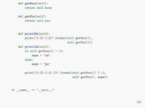
def getHour(self):return self.hour

def getMin(self):return self.min

def print24h(self):print("{:2}:{:2}".format(self.getHour(),

self.getMin()))def print12h(self):

if self.getHour() < 12:ampm = "am"

else:ampm = "pm"

print("{:2}:{:2} {}".format(self.getHour() % 12,self.getMin(), ampm))

if __name__ == "__main__":

382

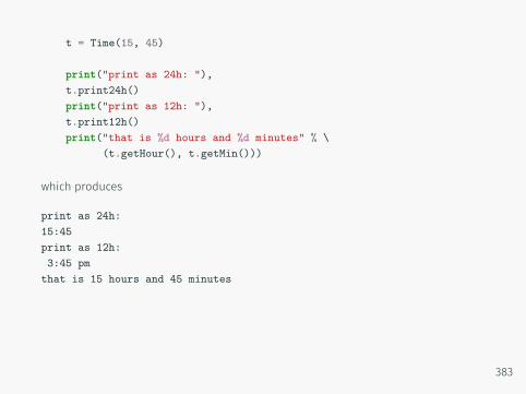
t = Time(15, 45)

print("print as 24h: "),t.print24h()print("print as 12h: "),t.print12h()print("that is %d hours and %d minutes" % \

(t.getHour(), t.getMin()))

which produces

print as 24h:15:45print as 12h:3:45 pmthat is 15 hours and 45 minutes

383

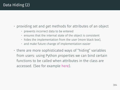
Data Hiding (2)

• providing set and get methods for attributes of an object• prevents incorrect data to be entered• ensures that the internal state of the object is consistent• hides the implementation from the user (more black box),• and make future change of implementation easier

• there are more sophisticated ways of “hiding” variablesfrom users: using Python properties we can bind certainfunctions to be called when attributes in the class areaccessed. (See for example here).

384

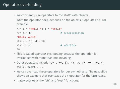
Operator overloading

• We constantly use operators to “do stuff” with objects.• What the operator does, depends on the objects it operates on. Forexample:>>> a = "Hello "; b = "World">>> a + b # concatenation'Hello World'>>> c = 10; d = 20>>> c + d # addition30

• This is called operator overloading because the operation isoverloaded with more than one meaning.

• Other operators include -,* , **, [], (), >, >=, ==, <=, <,str(), repr(), ...

• We can overload these operators for our own objects. The next slideshows an example that overloads the > operator for the Time class.

• It also overloads the “str” and “repr“ functions.385

class Time:def __init__(self, hour, min):

self.hour, self.min = hour, min

def __str__(self):"""overloading the str operator (STRing)"""return "[ %2d:%2d ]" % (self.hour, self.min)

def __repr__(self):"""overloading the repr operator (REPResentation)"""return "Time(%2d, %2d)" % (self.hour, self.min)

def __gt__(self, other):"""overloading the GreaTer operator"""selfminutes = self.hour * 60 + self.minotherminutes = other.hour * 60 + other.minif selfminutes > otherminutes:

return Trueelse:

return False

386

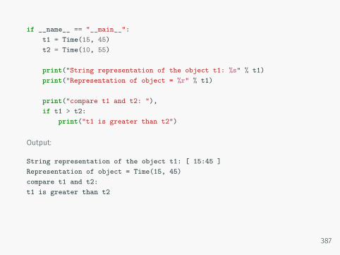
if __name__ == "__main__":t1 = Time(15, 45)t2 = Time(10, 55)

print("String representation of the object t1: %s" % t1)print("Representation of object = %r" % t1)

print("compare t1 and t2: "),if t1 > t2:

print("t1 is greater than t2")

Output:

String representation of the object t1: [ 15:45 ]Representation of object = Time(15, 45)compare t1 and t2:t1 is greater than t2

387

Inheritance

• Sometimes, we need classes that share certain (or verymany, or all) attributes but are slightly different.

• Example 1: Geometry• a point (in 2 dimensions) has an x and y attribute• a circle is a point with a radius• a cylinder is a circle with a height

• Example 2: People at universities• A person has an address.• A student is a person and selects modules.• A lecturer is a person with teaching duties.• …

• In these cases, we define a base class and derive otherclasses from it.

• This is called inheritance. The next slides show examples

388

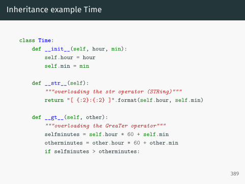
Inheritance example Time

class Time:def __init__(self, hour, min):

self.hour = hourself.min = min

def __str__(self):"""overloading the str operator (STRing)"""return "[ {:2}:{:2} ]".format(self.hour, self.min)

def __gt__(self, other):"""overloading the GreaTer operator"""selfminutes = self.hour * 60 + self.minotherminutes = other.hour * 60 + other.minif selfminutes > otherminutes:

389

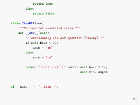
return Trueelse:

return False

class TimeUK(Time):"""Derived (or inherited class)"""def __str__(self):

"""overloading the str operator (STRing)"""if self.hour < 12:

ampm = "am"else:

ampm = "pm"

return "[{:2}:{:2}{}]".format(self.hour % 12,self.min, ampm)

if __name__ == "__main__":

390

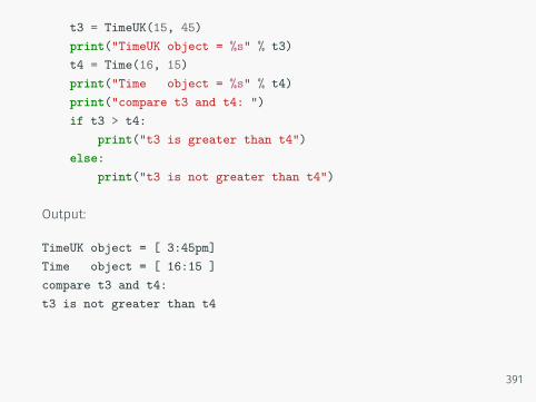
t3 = TimeUK(15, 45)print("TimeUK object = %s" % t3)t4 = Time(16, 15)print("Time object = %s" % t4)print("compare t3 and t4: ")if t3 > t4:

print("t3 is greater than t4")else:

print("t3 is not greater than t4")

Output:

TimeUK object = [ 3:45pm]Time object = [ 16:15 ]compare t3 and t4:t3 is not greater than t4

391

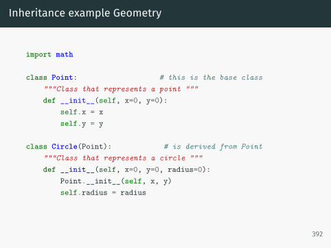
Inheritance example Geometry

import math

class Point: # this is the base class"""Class that represents a point """def __init__(self, x=0, y=0):

self.x = xself.y = y

class Circle(Point): # is derived from Point"""Class that represents a circle """def __init__(self, x=0, y=0, radius=0):

Point.__init__(self, x, y)self.radius = radius

392

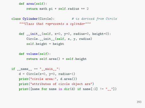
def area(self):return math.pi * self.radius ** 2

class Cylinder(Circle): # is derived from Circle"""Class that represents a cylinder"""

def __init__(self, x=0, y=0, radius=0, height=0):Circle.__init__(self, x, y, radius)self.height = height

def volume(self):return self.area() * self.height

if __name__ == "__main__":d = Circle(x=0, y=0, radius=1)print("circle area:", d.area())print("attributes of circle object are")print([name for name in dir(d) if name[:2] != "__"])

393

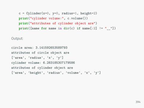
c = Cylinder(x=0, y=0, radius=1, height=2)print("cylinder volume:", c.volume())print("attributes of cylinder object are")print([name for name in dir(c) if name[:2] != "__"])

Output:

circle area: 3.141592653589793attributes of circle object are['area', 'radius', 'x', 'y']cylinder volume: 6.283185307179586attributes of cylinder object are['area', 'height', 'radius', 'volume', 'x', 'y']

394

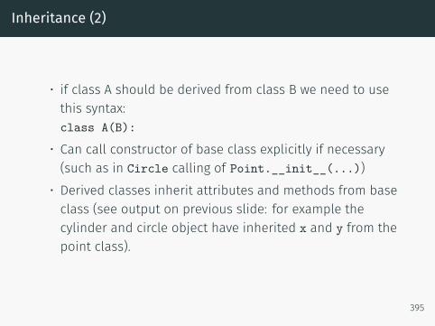
Inheritance (2)

• if class A should be derived from class B we need to usethis syntax:class A(B):

• Can call constructor of base class explicitly if necessary(such as in Circle calling of Point.__init__(...))

• Derived classes inherit attributes and methods from baseclass (see output on previous slide: for example thecylinder and circle object have inherited x and y from thepoint class).

395

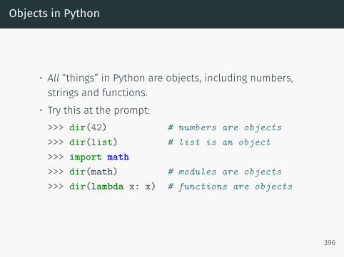
Objects in Python

• All “things” in Python are objects, including numbers,strings and functions.

• Try this at the prompt:>>> dir(42) # numbers are objects>>> dir(list) # list is an object>>> import math>>> dir(math) # modules are objects>>> dir(lambda x: x) # functions are objects

396

Summary Object Oriented Programming

Summary

• Object orientation is about merging data and functionsinto one object.

• There is a number of helpful concepts, including datahiding and operator overloading.

• Classes can provide get and set methods and hide theirimplementation.

• Classes can be derived from other classes.

397

Some software engineering observations

• OOP needs some time to get used to.• Good use of OOP

• makes large codes easier to maintain,• encourages re-use of existing code,• requires some thought (finding the right classes for a givenproblem can be difficult).

Note: Fortran 2003 supports Object Oriented Programming.

398

398

Some programming languages

Some Programming Languagesfor Computational Science

see also: http://www.levenez.com/lang/for an overview of general programming languages

400

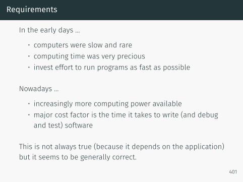
Requirements

In the early days …

• computers were slow and rare• computing time was very precious• invest effort to run programs as fast as possible

Nowadays …

• increasingly more computing power available• major cost factor is the time it takes to write (and debugand test) software

This is not always true (because it depends on the application)but it seems to be generally correct.

401

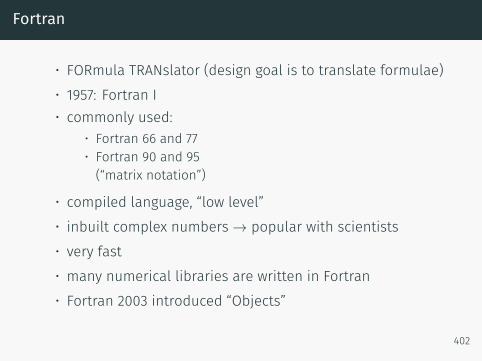
Fortran

• FORmula TRANslator (design goal is to translate formulae)• 1957: Fortran I• commonly used:

• Fortran 66 and 77• Fortran 90 and 95(“matrix notation”)

• compiled language, “low level”• inbuilt complex numbers→ popular with scientists• very fast• many numerical libraries are written in Fortran• Fortran 2003 introduced “Objects”

402

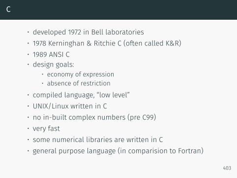
C

• developed 1972 in Bell laboratories• 1978 Kerninghan & Ritchie C (often called K&R)• 1989 ANSI C• design goals:

• economy of expression• absence of restriction

• compiled language, “low level”• UNIX/Linux written in C• no in-built complex numbers (pre C99)• very fast• some numerical libraries are written in C• general purpose language (in comparision to Fortran)

403

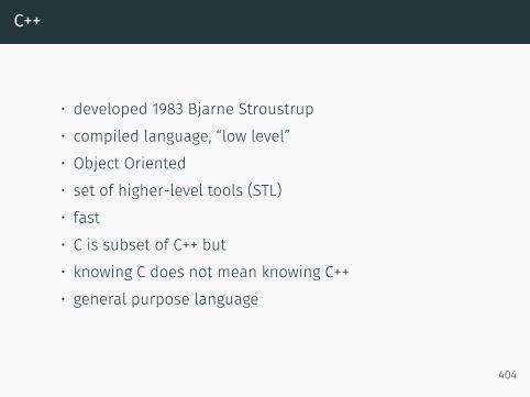
C++

• developed 1983 Bjarne Stroustrup• compiled language, “low level”• Object Oriented• set of higher-level tools (STL)• fast• C is subset of C++ but• knowing C does not mean knowing C++• general purpose language

404

MATLAB

• MATrix LABoratory (1984)• started as collection of linear algebra functions• scripting language grew to combine these functions• visualisation features were added• this is what we call MATLAB today• the MATLAB scripting language is interpreted and slow• the numerical libraries that come with MATLAB arecompiled and fast

• designed for numerical work (and very good at this)• can be fast if used carefully• “high-level language”→ higher coding efficiency• commercial product

• need to pay• users can not see (and check) source code

• very popular in engineering community 405

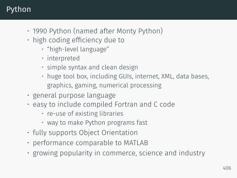
Python

• 1990 Python (named after Monty Python)• high coding efficiency due to

• “high-level language”• interpreted• simple syntax and clean design• huge tool box, including GUIs, internet, XML, data bases,graphics, gaming, numerical processing

• general purpose language• easy to include compiled Fortran and C code

• re-use of existing libraries• way to make Python programs fast

• fully supports Object Orientation• performance comparable to MATLAB• growing popularity in commerce, science and industry

406

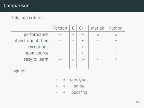
Comparison

Selected criteria:

Fortran C C++ Matlab Pythonperformance + + + ◦ ◦

object orientation – – + – +exceptions – – + – +

open source + + + – +easy to learn ◦+ ◦ ◦– + +

legend:

+ = good/yes◦ = so-so– = poor/no

407

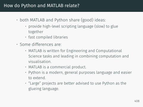
How do Python and MATLAB relate?

• both MATLAB and Python share (good) ideas:• provide high-level scripting language (slow) to gluetogether

• fast compiled libraries

• Some differences are:• MATLAB is written for Engineering and ComputationalScience tasks and leading in combining computation andvisualisation.

• MATLAB is a commercial product.• Python is a modern, general purposes language and easierto extend.

• “Large” projects are better advised to use Python as theglueing language.

408

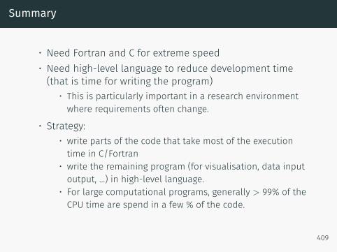
Summary

• Need Fortran and C for extreme speed• Need high-level language to reduce development time(that is time for writing the program)

• This is particularly important in a research environmentwhere requirements often change.

• Strategy:• write parts of the code that take most of the executiontime in C/Fortran

• write the remaining program (for visualisation, data inputoutput, …) in high-level language.

• For large computational programs, generally > 99% of theCPU time are spend in a few % of the code.

409

409

What language to learn next?

What language to learn next?

• …it all depends what you want to achieve:

• To learn C or Fortran, get a book or on-line tutorial.

• To learn object oriented programming (OOP), read “How to think like acomputer Scientist” (for Python), or try “Python – how to program” (seenext slides).

• To learn C++, learn OOP using Python first, then switch to C++.

• To learn Java or C#, you should consider learning OOP using Pythonfirst (but you could risk switching language straight away).

Note:

• Python provides an excellent platform for all possible tasks

⇒ it could well be all you need for some time to come.

411

Further reading

• “How to Think Like a ComputerScientist: Learning with Python”.(ISBN 0971677506) free athttp://greenteapress.com/wp/think-python-2e/

• Very systematic presentation ofall important programmingconcepts, including OOP.

• Aimed at first year computerscience students.

• Recommended if you likeprogramming and want to knowmore about the concepts.

412

Other tools and topics

Tools to extend your computational toolkit / suggestedself-study topics

• Systematic testing (py.test or nose) and• Test Driven Development (TDD)• Version control (try Mercurial or Git)• Automate everything• IPython Notebook• LATEX (professional document creation)• Cool editor (Emacs? Sublime? ...)

413

Acknowledgements

Thanks go to Ondrej Hovorka and Neil O’Brien for contributingto these slides.

414