
Computational Geometry Aspects of Monte Carlo Approaches ...
Computational Physics: An Introduction to
Monte Carlo Simulations of Matrix Field Theory
Badis Ydri
Department of Physics, Faculty of Sciences, BM Annaba University,
Annaba, Algeria.
March 16, 2016
Abstract
This book is divided into two parts. In the first part we give an elementary introduc-
tion to computational physics consisting of 21 simulations which originated from a formal
course of lectures and laboratory simulations delivered since 2010 to physics students at
Annaba University. The second part is much more advanced and deals with the problem
of how to set up working Monte Carlo simulations of matrix field theories which involve fi-
nite dimensional matrix regularizations of noncommutative and fuzzy field theories, fuzzy
spaces and matrix geometry. The study of matrix field theory in its own right has also
become very important to the proper understanding of all noncommutative, fuzzy and
matrix phenomena. The second part, which consists of 9 simulations, was delivered infor-
mally to doctoral students who are working on various problems in matrix field theory.
Sample codes as well as sample key solutions are also provided for convenience and com-
pletness. An appendix containing an executive arabic summary of the first part is added
at the end of the book.
arX
iv:1
506.
0256
7v2
[he
p-la
t] 1
5 M
ar 2
016
Contents
Introductory Remarks 8
Introducing Computational Physics . . . . . . . . . . . . . . . . . . . . . . . . . 8
References . . . . . . . . . . . . . . . . . . . . . . . . . . . . . . . . . . . . . . . 9
Codes and Solutions . . . . . . . . . . . . . . . . . . . . . . . . . . . . . . . . . 9
Matrix Field Theory . . . . . . . . . . . . . . . . . . . . . . . . . . . . . . . . . 9
Appendices . . . . . . . . . . . . . . . . . . . . . . . . . . . . . . . . . . . . . . 10
Acknowledgments . . . . . . . . . . . . . . . . . . . . . . . . . . . . . . . . . . . 10
I Introduction to Computational Physics 11
1 Euler Algorithm 12
1.1 Euler Algorithm . . . . . . . . . . . . . . . . . . . . . . . . . . . . . . . . 12
1.2 First Example and Sample Code . . . . . . . . . . . . . . . . . . . . . . . 13
1.2.1 Radioactive Decay . . . . . . . . . . . . . . . . . . . . . . . . . . . 13
1.2.2 A Sample Fortran Code . . . . . . . . . . . . . . . . . . . . . . . . 15
1.3 More Examples . . . . . . . . . . . . . . . . . . . . . . . . . . . . . . . . . 16
1.3.1 Air Resistance . . . . . . . . . . . . . . . . . . . . . . . . . . . . . 16
1.3.2 Projectile Motion . . . . . . . . . . . . . . . . . . . . . . . . . . . . 18
1.4 Periodic Motions and Euler-Cromer and Verlet Algorithms . . . . . . . . 19
1.4.1 Harmonic Oscillator . . . . . . . . . . . . . . . . . . . . . . . . . . 20
1.4.2 Euler Algorithm . . . . . . . . . . . . . . . . . . . . . . . . . . . . 20
1.4.3 Euler-Cromer Algorithm . . . . . . . . . . . . . . . . . . . . . . . . 21
1.4.4 Verlet Algorithm . . . . . . . . . . . . . . . . . . . . . . . . . . . . 22
1.5 Exercises . . . . . . . . . . . . . . . . . . . . . . . . . . . . . . . . . . . . 23
1.6 Simulation 1: Euler Algorithm- Air Resistance . . . . . . . . . . . . . . . 24
1.7 Simulation 2: Euler Algorithm- Projectile Motion . . . . . . . . . . . . . . 24
1.8 Simulation 3: Euler, Euler-Cromer and Verlet Algorithms . . . . . . . . . 25
2 Classical Numerical Integration 27
2.1 Rectangular Approximation . . . . . . . . . . . . . . . . . . . . . . . . . . 27
2.2 Trapezoidal Approximation . . . . . . . . . . . . . . . . . . . . . . . . . . 28
2.3 Parabolic Approximation or Simpson’s Rule . . . . . . . . . . . . . . . . . 28
2.4 Errors . . . . . . . . . . . . . . . . . . . . . . . . . . . . . . . . . . . . . . 30

CP and MFT, B.Ydri 3
2.5 Simulation 4: Numerical Integrals . . . . . . . . . . . . . . . . . . . . . . . 31
3 Newton-Raphson Algorithms and Interpolation 32
3.1 Bisection Algorithm . . . . . . . . . . . . . . . . . . . . . . . . . . . . . . 32
3.2 Newton-Raphson Algorithm . . . . . . . . . . . . . . . . . . . . . . . . . . 32
3.3 Hybrid Method . . . . . . . . . . . . . . . . . . . . . . . . . . . . . . . . . 34
3.4 Lagrange Interpolation . . . . . . . . . . . . . . . . . . . . . . . . . . . . . 34
3.5 Cubic Spline Interpolation . . . . . . . . . . . . . . . . . . . . . . . . . . . 36
3.6 The Method of Least Squares . . . . . . . . . . . . . . . . . . . . . . . . . 37
3.7 Simulation 5: Newton-Raphson Algorithm . . . . . . . . . . . . . . . . . . 38
4 The Solar System-The Runge-Kutta Methods 39
4.1 The Solar System . . . . . . . . . . . . . . . . . . . . . . . . . . . . . . . . 39
4.1.1 Newton’s Second Law . . . . . . . . . . . . . . . . . . . . . . . . . 39
4.1.2 Astronomical Units and Initial Conditions . . . . . . . . . . . . . . 40
4.1.3 Kepler’s Laws . . . . . . . . . . . . . . . . . . . . . . . . . . . . . . 41
4.1.4 The inverse-Square Law and Stability of Orbits . . . . . . . . . . . 43
4.2 Euler-Cromer Algorithm . . . . . . . . . . . . . . . . . . . . . . . . . . . . 43
4.3 The Runge-Kutta Algorithm . . . . . . . . . . . . . . . . . . . . . . . . . 44
4.3.1 The Method . . . . . . . . . . . . . . . . . . . . . . . . . . . . . . 44
4.3.2 Example 1: The Harmonic Oscillator . . . . . . . . . . . . . . . . . 45
4.3.3 Example 2: The Solar System . . . . . . . . . . . . . . . . . . . . . 46
4.4 Precession of the Perihelion of Mercury . . . . . . . . . . . . . . . . . . . 47
4.5 Exercises . . . . . . . . . . . . . . . . . . . . . . . . . . . . . . . . . . . . 48
4.6 Simulation 6: Runge-Kutta Algorithm- The Solar System . . . . . . . . . 49
4.7 Simulation 7: Precession of the perihelion of Mercury . . . . . . . . . . . 50
5 Chaotic Pendulum 52
5.1 Equation of Motion . . . . . . . . . . . . . . . . . . . . . . . . . . . . . . . 52
5.2 Numerical Algorithms . . . . . . . . . . . . . . . . . . . . . . . . . . . . . 54
5.2.1 Euler-Cromer Algorithm . . . . . . . . . . . . . . . . . . . . . . . . 54
5.2.2 Runge-Kutta Algorithm . . . . . . . . . . . . . . . . . . . . . . . . 55
5.3 Elements of Chaos . . . . . . . . . . . . . . . . . . . . . . . . . . . . . . . 56
5.3.1 Butterfly Effect: Sensitivity to Initial Conditions . . . . . . . . . . 56
5.3.2 Poincare Section and Attractors . . . . . . . . . . . . . . . . . . . 57
5.3.3 Period-Doubling Bifurcations . . . . . . . . . . . . . . . . . . . . . 57
5.3.4 Feigenbaum Ratio . . . . . . . . . . . . . . . . . . . . . . . . . . . 58
5.3.5 Spontaneous Symmetry Breaking . . . . . . . . . . . . . . . . . . . 58
5.4 Simulation 8: The Butterfly Effect . . . . . . . . . . . . . . . . . . . . . . 59
5.5 Simulation 9: Poincare Sections . . . . . . . . . . . . . . . . . . . . . . . . 59
5.6 Simulation 10: Period Doubling . . . . . . . . . . . . . . . . . . . . . . . . 61
5.7 Simulation 11: Bifurcation Diagrams . . . . . . . . . . . . . . . . . . . . . 61
CP and MFT, B.Ydri 4
6 Molecular Dynamics 64
6.1 Introduction . . . . . . . . . . . . . . . . . . . . . . . . . . . . . . . . . . . 64
6.2 The Lennard-Jones Potential . . . . . . . . . . . . . . . . . . . . . . . . . 64
6.3 Units, Boundary Conditions and Verlet Algorithm . . . . . . . . . . . . . 66
6.4 Some Physical Applications . . . . . . . . . . . . . . . . . . . . . . . . . . 68
6.4.1 Dilute Gas and Maxwell Distribution . . . . . . . . . . . . . . . . . 68
6.4.2 The Melting Transition . . . . . . . . . . . . . . . . . . . . . . . . 69
6.5 Simulation 12: Maxwell Distribution . . . . . . . . . . . . . . . . . . . . . 69
6.6 Simulation 13: Melting Transition . . . . . . . . . . . . . . . . . . . . . . 70
7 Pseudo Random Numbers and Random Walks 71
7.1 Random Numbers . . . . . . . . . . . . . . . . . . . . . . . . . . . . . . . 71
7.1.1 Linear Congruent or Power Residue Method . . . . . . . . . . . . . 71
7.1.2 Statistical Tests of Randomness . . . . . . . . . . . . . . . . . . . . 72
7.2 Random Systems . . . . . . . . . . . . . . . . . . . . . . . . . . . . . . . . 74
7.2.1 Random Walks . . . . . . . . . . . . . . . . . . . . . . . . . . . . . 74
7.2.2 Diffusion Equation . . . . . . . . . . . . . . . . . . . . . . . . . . . 76
7.3 The Random Number Generators RAN 0, 1, 2 . . . . . . . . . . . . . . . . 77
7.4 Simulation 14: Random Numbers . . . . . . . . . . . . . . . . . . . . . . . 80
7.5 Simulation 15: Random Walks . . . . . . . . . . . . . . . . . . . . . . . . 81
8 Monte Carlo Integration 83
8.1 Numerical Integration . . . . . . . . . . . . . . . . . . . . . . . . . . . . . 83
8.1.1 Rectangular Approximation Revisted . . . . . . . . . . . . . . . . . 83
8.1.2 Midpoint Approximation of Multidimensional Integrals . . . . . . 84
8.1.3 Spheres and Balls in d Dimensions . . . . . . . . . . . . . . . . . . 86
8.2 Monte Carlo Integration: Simple Sampling . . . . . . . . . . . . . . . . . . 86
8.2.1 Sampling (Hit or Miss) Method . . . . . . . . . . . . . . . . . . . . 87
8.2.2 Sample Mean Method . . . . . . . . . . . . . . . . . . . . . . . . . 87
8.2.3 Sample Mean Method in Higher Dimensions . . . . . . . . . . . . . 87
8.3 The Central Limit Theorem . . . . . . . . . . . . . . . . . . . . . . . . . . 88
8.4 Monte Carlo Errors and Standard Deviation . . . . . . . . . . . . . . . . . 90
8.5 Nonuniform Probability Distributions . . . . . . . . . . . . . . . . . . . . 92
8.5.1 The Inverse Transform Method . . . . . . . . . . . . . . . . . . . . 92
8.5.2 The Acceptance-Rejection Method . . . . . . . . . . . . . . . . . . 94
8.6 Simulation 16: Midpoint and Monte Carlo Approximations . . . . . . . . 94
8.7 Simulation 17: Nonuniform Probability Distributions . . . . . . . . . . . . 96
9 The Metropolis Algorithm and The Ising Model 98
9.1 The Canonical Ensemble . . . . . . . . . . . . . . . . . . . . . . . . . . . . 98
9.2 Importance Sampling . . . . . . . . . . . . . . . . . . . . . . . . . . . . . . 99
9.3 The Ising Model . . . . . . . . . . . . . . . . . . . . . . . . . . . . . . . . 100
9.4 The Metropolis Algorithm . . . . . . . . . . . . . . . . . . . . . . . . . . . 101
9.5 The Heat-Bath Algorithm . . . . . . . . . . . . . . . . . . . . . . . . . . . 103
CP and MFT, B.Ydri 5
9.6 The Mean Field Approximation . . . . . . . . . . . . . . . . . . . . . . . . 103
9.6.1 Phase Diagram and Critical Temperature . . . . . . . . . . . . . . 103
9.6.2 Critical Exponents . . . . . . . . . . . . . . . . . . . . . . . . . . . 105
9.7 Simulation of The Ising Model and Numerical Results . . . . . . . . . . . 107
9.7.1 The Fortran Code . . . . . . . . . . . . . . . . . . . . . . . . . . . 107
9.7.2 Some Numerical Results . . . . . . . . . . . . . . . . . . . . . . . . 109
9.8 Simulation 18: The Metropolis Algorithm and The Ising Model . . . . . . 111
9.9 Simulation 19: The Ferromagnetic Second Order Phase Transition . . . . 112
9.10 Simulation 20: The 2−Point Correlator . . . . . . . . . . . . . . . . . . . 113
9.11 Simulation 21: Hysteresis and The First Order Phase Transition . . . . . 113
II Monte Carlo Simulations of Matrix Field Theory 115
1 Metropolis Algorithm for Yang-Mills Matrix Models 116
1.1 Dimensional Reduction . . . . . . . . . . . . . . . . . . . . . . . . . . . . . 116
1.1.1 Yang-Mills Action . . . . . . . . . . . . . . . . . . . . . . . . . . . 116
1.1.2 Chern-Simons Action: Myers Term . . . . . . . . . . . . . . . . . . 118
1.2 Metropolis Accept/Reject Step . . . . . . . . . . . . . . . . . . . . . . . . 122
1.3 Statistical Errors . . . . . . . . . . . . . . . . . . . . . . . . . . . . . . . . 123
1.4 Auto-Correlation Time . . . . . . . . . . . . . . . . . . . . . . . . . . . . . 123
1.5 Code and Sample Calculation . . . . . . . . . . . . . . . . . . . . . . . . . 125
2 Hybrid Monte Carlo Algorithm for Yang-Mills Matrix Models 128
2.1 The Yang-Mills Matrix Action . . . . . . . . . . . . . . . . . . . . . . . . 128
2.2 The Leap Frog Algorithm . . . . . . . . . . . . . . . . . . . . . . . . . . . 129
2.3 Metropolis Algorithm . . . . . . . . . . . . . . . . . . . . . . . . . . . . . 131
2.4 Gaussian Distribution . . . . . . . . . . . . . . . . . . . . . . . . . . . . . 132
2.5 Physical Tests . . . . . . . . . . . . . . . . . . . . . . . . . . . . . . . . . . 132
2.6 Emergent Geometry: An Exotic Phase Transition . . . . . . . . . . . . . . 134
3 Hybrid Monte Carlo Algorithm for Noncommutative Phi-Four 141
3.1 The Matrix Scalar Action . . . . . . . . . . . . . . . . . . . . . . . . . . . 141
3.2 The Leap Frog Algorithm . . . . . . . . . . . . . . . . . . . . . . . . . . . 142
3.3 Hybrid Monte Carlo Algorithm . . . . . . . . . . . . . . . . . . . . . . . . 142
3.4 Optimization . . . . . . . . . . . . . . . . . . . . . . . . . . . . . . . . . . 143
3.4.1 Partial Optimization . . . . . . . . . . . . . . . . . . . . . . . . . . 143
3.4.2 Full Optimization . . . . . . . . . . . . . . . . . . . . . . . . . . . 145
3.5 The Non-Uniform Order: Another Exotic Phase . . . . . . . . . . . . . . . 145
3.5.1 Phase Structure . . . . . . . . . . . . . . . . . . . . . . . . . . . . 145
3.5.2 Sample Simulations . . . . . . . . . . . . . . . . . . . . . . . . . . 146

CP and MFT, B.Ydri 6
4 Lattice HMC Simulations of Φ42: A Lattice Example 157
4.1 Model and Phase Structure . . . . . . . . . . . . . . . . . . . . . . . . . . 157
4.2 The HM Algorithm . . . . . . . . . . . . . . . . . . . . . . . . . . . . . . . 161
4.3 Renormalization and Continuum Limit . . . . . . . . . . . . . . . . . . . . 163
4.4 HMC Simulation Calculation of The Critical Line . . . . . . . . . . . . . . 165
5 (Multi-Trace) Quartic Matrix Models 170
5.1 The Pure Real Quartic Matrix Model . . . . . . . . . . . . . . . . . . . . 170
5.2 The Multi-Trace Matrix Model . . . . . . . . . . . . . . . . . . . . . . . . 171
5.3 Model and Algorithm . . . . . . . . . . . . . . . . . . . . . . . . . . . . . 173
5.4 The Disorder-to-Non-Uniform-Order Transition . . . . . . . . . . . . . . . 175
5.5 Other Suitable Algorithms . . . . . . . . . . . . . . . . . . . . . . . . . . . 177
5.5.1 Over-Relaxation Algorithm . . . . . . . . . . . . . . . . . . . . . . 177
5.5.2 Heat-Bath Algorithm . . . . . . . . . . . . . . . . . . . . . . . . . 178
6 The Remez Algorithm and The Conjugate Gradient Method 181
6.1 Minimax Approximations . . . . . . . . . . . . . . . . . . . . . . . . . . . 181
6.1.1 Minimax Polynomial Approximation and Chebyshev Polynomials . 181
6.1.2 Minimax Rational Approximation and Remez Algorithm . . . . . . 186
6.1.3 The Code ”AlgRemez” . . . . . . . . . . . . . . . . . . . . . . . . . 189
6.2 Conjugate Gradient Method . . . . . . . . . . . . . . . . . . . . . . . . . . 189
6.2.1 Construction . . . . . . . . . . . . . . . . . . . . . . . . . . . . . . 189
6.2.2 The Conjugate Gradient Method as a Krylov Space Solver . . . . . 193
6.2.3 The Multi-Mass Conjugate Gradient Method . . . . . . . . . . . . 195
7 Monte Carlo Simulation of Fermion Determinants 199
7.1 The Dirac Operator . . . . . . . . . . . . . . . . . . . . . . . . . . . . . . 199
7.2 Pseudo-Fermions and Rational Approximations . . . . . . . . . . . . . . . 203
7.3 More on The Conjugate-Gradient . . . . . . . . . . . . . . . . . . . . . . . 205
7.3.1 Multiplication by M′and (M′
)+ . . . . . . . . . . . . . . . . . . . 205
7.3.2 The Fermionic Force . . . . . . . . . . . . . . . . . . . . . . . . . . 208
7.4 The Rational Hybrid Monte Carlo Algorithm . . . . . . . . . . . . . . . . 210
7.4.1 Statement . . . . . . . . . . . . . . . . . . . . . . . . . . . . . . . . 210
7.4.2 Preliminary Tests . . . . . . . . . . . . . . . . . . . . . . . . . . . . 211
7.5 Other Related Topics . . . . . . . . . . . . . . . . . . . . . . . . . . . . . . 218
8 U(1) Gauge Theory on the Lattice: Another Lattice Example 220
8.1 Continuum Considerations . . . . . . . . . . . . . . . . . . . . . . . . . . . 220
8.2 Lattice Regularization . . . . . . . . . . . . . . . . . . . . . . . . . . . . . 222
8.2.1 Lattice Fermions and Gauge Fields . . . . . . . . . . . . . . . . . . 222
8.2.2 Quenched Approximation . . . . . . . . . . . . . . . . . . . . . . . 225
8.2.3 Wilson Loop, Creutz Ratio and Other Observables . . . . . . . . . 226
8.3 Monte Carlo Simulation of Pure U(1) Gauge Theory . . . . . . . . . . . . 228
8.3.1 The Metropolis Algorithm . . . . . . . . . . . . . . . . . . . . . . . 228
CP and MFT, B.Ydri 7
8.3.2 Some Numerical Results . . . . . . . . . . . . . . . . . . . . . . . . 231
8.3.3 Coulomb and Confinement Phases . . . . . . . . . . . . . . . . . . 232
9 Codes 237
9.1 metropolis-ym.f . . . . . . . . . . . . . . . . . . . . . . . . . . . . . . . . . . 238
9.2 hybrid-ym.f . . . . . . . . . . . . . . . . . . . . . . . . . . . . . . . . . . . . 244
9.3 hybrid-scalar-fuzzy.f . . . . . . . . . . . . . . . . . . . . . . . . . . . . . . . 251
9.4 phi-four-on-lattice.f . . . . . . . . . . . . . . . . . . . . . . . . . . . . . . . . 261
9.5 metropolis-scalar-multitrace.f . . . . . . . . . . . . . . . . . . . . . . . . . . 268
9.6 remez.f . . . . . . . . . . . . . . . . . . . . . . . . . . . . . . . . . . . . . . 275
9.7 conjugate-gradient.f . . . . . . . . . . . . . . . . . . . . . . . . . . . . . . . 277
9.8 hybrid-supersymmetric-ym.f . . . . . . . . . . . . . . . . . . . . . . . . . . . 280
9.9 u-one-on-the-lattice.f . . . . . . . . . . . . . . . . . . . . . . . . . . . . . . . 298
A Floating Point Representation, Machine Precision and Errors 309
B Executive Arabic Summary of Part I 313
Introductory Remarks
Introducing Computational Physics
Computational physics is a subfield of computational science and scientific computing
in which we combine elements from physics (especially theoretical), elements from mathe-
matics (in particular applied mathematics such as numerical analysis) and elements from
computer science (programming) for the purpose of solving a physics problem. In physics
there are traditionally two approaches which are followed: 1) The experimental approach
and 2) The theoretical approach. Nowadays, we may consider “The computational ap-
proach” as a third approach in physics. It can even be argued that the computational
approach is independent from the first two approaches and it is not simply a bridge be-
tween the two.
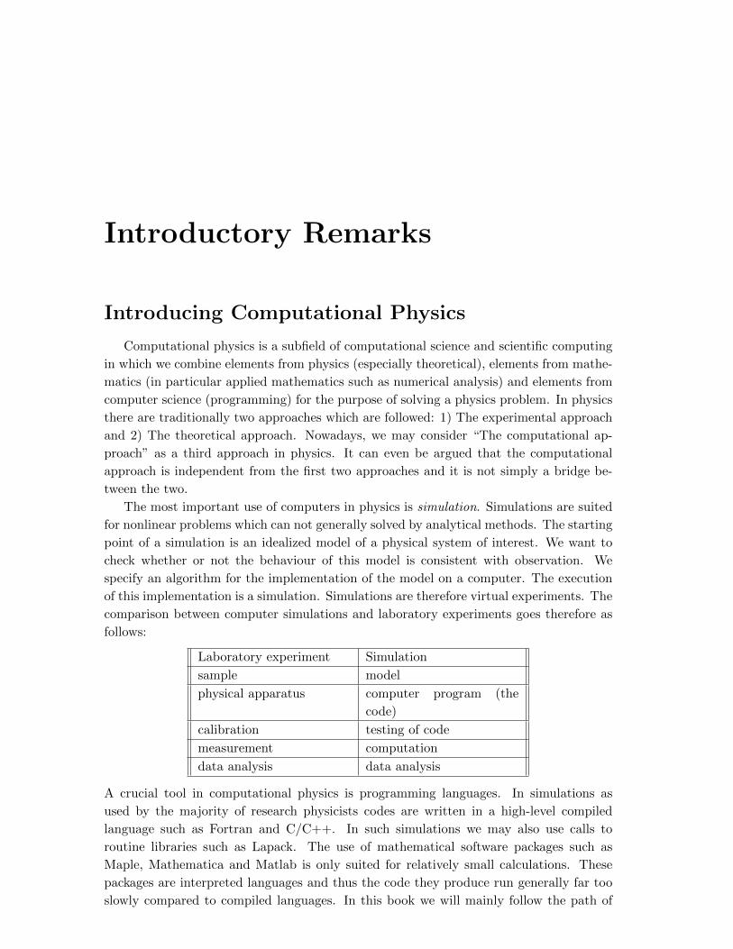
The most important use of computers in physics is simulation. Simulations are suited
for nonlinear problems which can not generally solved by analytical methods. The starting
point of a simulation is an idealized model of a physical system of interest. We want to
check whether or not the behaviour of this model is consistent with observation. We
specify an algorithm for the implementation of the model on a computer. The execution
of this implementation is a simulation. Simulations are therefore virtual experiments. The
comparison between computer simulations and laboratory experiments goes therefore as
follows:
Laboratory experiment Simulation
sample model
physical apparatus computer program (the
code)
calibration testing of code
measurement computation
data analysis data analysis
A crucial tool in computational physics is programming languages. In simulations as
used by the majority of research physicists codes are written in a high-level compiled
language such as Fortran and C/C++. In such simulations we may also use calls to
routine libraries such as Lapack. The use of mathematical software packages such as
Maple, Mathematica and Matlab is only suited for relatively small calculations. These
packages are interpreted languages and thus the code they produce run generally far too
slowly compared to compiled languages. In this book we will mainly follow the path of
CP and MFT, B.Ydri 9
developping and writing all our codes in a high-level compiled language and not call any
libraries. As our programming language we will use Fortran 77 under the Linux operating
system. We adopt exclusively the Ubuntu distribution of Linux. We will use the Fortran
compilers f77 and gfortran. As an editor we will use mostly Emacs and sometimes Gedit
and Nano while for graphics we will use mostly Gnuplot.
References
The main references which we have followed in developing the first part of this book
include the following items:
1. N.J.Giordano, H. Nakanishi, Computational Physics (2nd edition), Pearson/Prentice
Hall, (2006).
2. H.Gould, J.Tobochnick, W.Christian, An Introduction To Computer Simulation
Methods: Applications to Physical Systems (3rd Edition), Addison-Wesley (2006).
3. R.H.Landau, M.J.Paez, C.C. Bordeianu, Computational Physics: Problem Solving
with Computers (2nd edition), John Wiley and Sons (2007).
4. R.Fitzpatrick, Introduction to Computational Physics,
http://farside.ph.utexas.edu/teaching/329/329.html.
5. Konstantinos Anagnostopoulos, Computational Physics: A Practical Introduction
to Computational Physics and Scientific Computing, Lulu.com (2014).
6. J. M. Thijssen, Computational Physics, Cambridge University Press (1999).
7. M. Hjorth-Jensen,Computational Physics, CreateSpace Publishing (2015).
8. Paul L.DeVries, A First Course in Computational Physics (2nd edition), Jones and
Bartlett Publishers (2010).
Codes and Solutions
The Fortran codes relevant to the problems considered in the first part of the book as
well as some key sample solutions can be found at the URL:
http://homepages.dias.ie/ydri/codes_solutions/
Matrix Field Theory
The second part of this book, which is effectively the main part, deals with the impor-
tant problem of how to set up working Monte Carlo simulations of matrix field theories in
a, hopefully, pedagogical way. The subject of matrix field theory involves non-perturbative
matrix regularizations, or simply matrix representations, of noncommutative field theory
and noncommutative geometry, fuzzy physics and fuzzy spaces, fuzzy field theory, matrix
geometry and gravity and random matrix theory. The subject of matrix field theory may
CP and MFT, B.Ydri 10
even include matrix regularizations of supersymmetry, string theory and M-theory. These
matrix regularizations employ necessarily finite dimensional matrix algebras so that the
problems are amenable and are accessible to Monte Carlo methods.
The matrix regulator should be contrasted with the, well established, lattice regulator
with advantages and disadvantages which are discussed in their places in the literature.
However, we note that only 5 simulations among the 7 simulations considered in this part
of the book use the matrix regulator whereas the other 2, closely related simulations, use
the usual lattice regulator. This part contains also a special chapter on the Remez and
conjugate gradient algorithms which are required for the simulation of dynamical fermions.
The study of matrix field theory in its own right, and not thought of as regulator, has
also become very important to the proper understanding of all noncommutative, fuzzy
and matrix phenomena. Naturally, therefore, the mathematical, physical and numerical
aspects, required for the proper study of matrix field theory, which are found in this part
of the book are quite advanced by comparison with what is found in the first part of the
book.
The set of references for each topic consists mainly of research articles and is included
at the end of each chapter. Sample numerical calculations are also included as a section
or several sections in each chapter. Some of these solutions are quite detailed whereas
others are brief. The relevant Fortran codes for this part of the book are collected in the
last chapter for convenience and completeness. These codes are, of course, provided as is
and no warranty should be assumed.
Appendices
We attach two appendices at the end of this book relevant to the first part of this
book. In the first appendix we discuss the floating point representation of numbers,
machine precision and roundoff and systematic errors. In the second appendix we give an
executive summary of the simulations of part I translated into arabic.
Acknowledgments
Firstly, I would like to thank both the ex-head as well as the current-head of the
physics department, professor M.Benchihab and professor A.Chibani, for their critical
help in formally launching the computational physics course at BM Annaba University
during the academic year 2009-2010 and thus making the whole experience possible. This
three-semester course, based on the first part of this book, has become since a fixture
of the physics curriculum at both the Licence (Bachelor) and Master levels. Secondly, I
should also thank doctor A.Bouchareb and doctor R.Chemam who had helped in a crucial
way with the actual teaching of the course, especially the laboratory simulations, since the
beginning. Lastly, I would like to thank my doctoral students and doctor A.Bouchareb for
their patience and contributions during the development of the second part of this book
in the weekly informal meeting we have organized for this purpose.

Part I
Introduction to Computational
Physics

Chapter 1
Euler Algorithm
1.1 Euler Algorithm
It is a well appreciated fact that first order differential equations are commonplace in all
branches of physics. They appear virtually everywhere and some of the most fundamental
problems of nature obey simple first order differential equations or second order differential
equations. It is so often possible to recast second order differential equations as first order
differential equations with a doubled number of unknown. From the numerical standpoint
the problem of solving first order differential equations is a conceptually simple one as we
will now explain.
We consider the general first order ordinary differential equation
y′
=dy
dx= f(x, y). (1.1)
We impose the general initial-value boundary condition is
y(x0) = y0. (1.2)
We solve for the function y = y(x) in the unit x−interval starting from x0. We make the
x−interval discretization
xn = x0 + n∆x , n = 0, 1, ... (1.3)
The Euler algorithm is one of the oldest known numerical recipe. It consists in replacing
the function y(x) in the interval [xn, xn+1] by the straight line connecting the points
(xn, yn) and (xn+1, yn+1). This comes from the definition of the derivative at the point
x = xn given by
yn+1 − ynxn+1 − xn
= f(xn, yn). (1.4)
This means that we replace the above first order differential equation by the finite differ-
ence equation
yn+1 ' yn + ∆xf(xn, yn). (1.5)
CP and MFT, B.Ydri 13
This is only an approximation. The truncation error is given by the next term in the
Taylor’s expansion of the function y(x) which is given by
yn+1 ' yn + ∆xf(xn, yn) +1
2∆x2df(x, y)
dx|x=xn + .... (1.6)
The error then reads
1
2(∆x)2df(x, y)
dx|x=xn . (1.7)
The error per step is therefore proportional to (∆x)2. In a unit interval we will perform
N = 1/∆x steps. The total systematic error is therefore proportional to
N(∆x)2 =1
N. (1.8)
1.2 First Example and Sample Code
1.2.1 Radioactive Decay
It is an experimental fact that radioactive decay obeys a very simple first order differ-
ential equation. In a spontaneous radioactive decay a particle with no external influence
will decay into other particles. A typical example is the nuclear isotope uranium 235.
The exact moment of decay of any one particle is random. This means that the number
−dN (t) = N (t)−N (t+ dt) of nuclei which will decay during a time inetrval dt must be
proportional to dt and to the number N (t) of particles present at time t, i.e.
− dN (t) ∝ N (t)dt. (1.9)
In other words the probability of decay per unit time given by (−dN (t)/N (t))/dt is a
constant which we denote 1/τ . The minus sign is due to the fact that dN (t) is negative
since the number of particles decreases with time. We write
dN (t)
dt= −N (t)
τ. (1.10)
The solution of this first order differential equation is given by a simple exponential func-
tion, viz
N (t) = N0 exp(−t/τ). (1.11)
The number N0 is the number of particles at time t = 0. The time τ is called the mean
lifetime. It is the average time for decay. For the uranium 235 the mean lifetime is around
109 years.
The goal now is to obtain an approximate numerical solution to the problem of ra-
dioactivity using the Euler algorithm. In this particular case we can compare to an exact
solution given by the exponential decay law (1.11). We start evidently from the Taylor’s
expansion

CP and MFT, B.Ydri 14
N (t+ ∆t) = N (t) + ∆tdNdt
+1
2(∆t)2d
2Ndt2
+ ... (1.12)
We get in the limit ∆t −→ 0
dNdt
= Lim∆t−→0N (t+ ∆t)−N (t)
∆t. (1.13)
We take ∆t small but non zero. In this case we obtain the approximation
dNdt'N (t+ ∆t)−N (t)
∆t. (1.14)
Equivalently
N (t+ ∆t) ' N (t) + ∆tdNdt. (1.15)
By using (1.10) we get
N (t+ ∆t) ' N (t)−∆tN (t)
τ. (1.16)
We will start from the number of particles at time t = 0 given by N (0) = N0 which is
known. We substitute t = 0 in (1.16) to obtain N (∆t) = N (1) as a function of N (0).
Next the value N (1) can be used in equation (1.16) to get N (2∆t) = N (2), etc. We are
thus led to the time discretization
t ≡ t(i) = i∆t , i = 0, ..., N. (1.17)
In other words
N (t) = N (i). (1.18)
The integer N determine the total time interval T = N∆t. The numerical solution (1.16)
can be rewritten as
N (i+ 1) = N (i)−∆tN (i)
τ, i = 0, ..., N. (1.19)
This is Euler algorithm for radioactive decay. For convenience we shift the integer i so
that the above equation takes the form
N (i) = N (i− 1)−∆tN (i− 1)
τ, i = 1, ..., N + 1. (1.20)
We introduce N (i) = N (i− 1), i.e N (1) = N (0) = N0. We get
N (i+ 1) = N (i)−∆tN (i)
τ, i = 1, ..., N + 1. (1.21)
The corresponding times are
t(i+ 1) = i∆t , i = 1, ..., N + 1. (1.22)
The initial number of particles at time t(1) = 0 is N (1) = N0. This approximate solution
should be compared with the exact solution (1.11).
CP and MFT, B.Ydri 15
1.2.2 A Sample Fortran Code
The goal in this section is to provide a sample Fortran code which implements the above
algorithm (1.21). The reasons behind choosing Fortran were explained in the introduction.
Any Fortran program, like any other programing language, must start with some program
statement and conclude with an end statement. The program statement allows us to give
a name to the program. The end statement may be preceded by a return statement. This
looks like
program radioactivity
c Here is the code
return
end
We have chosen the name “radioactivity” for our program. The “c” in the second line
indicates that the sentence “here is the code” is only a comment and not a part of the
code.
After the program statement come the declaration statements. We state the variables
and their types which are used in the program. In Fortran we have the integer type for
integer variables and the double precision type for real variables. In the case of (1.21) the
variables N (i), t(i), τ , ∆t, N0 are real numbers while the variables i and N are integer
numbers.
An array A of dimension K is an ordered list of K variables of a given type called the
elements of the array and denoted A(1), A(2),...,A(K). In our above example N (i) and
t(i) are real arrays of dimension N + 1. We declare that N (i) and t(i) are real for all
i = 1, ..., N + 1 by writing N (1 : N + 1) and t(1 : N + 1).
Since an array is declared at the begining of the program it must have a fixed size. In
other words the upper limit must be a constant and not a variable. In Fortran a constant
is declared with a parameter statement. In our above case the upper limit is N + 1 and
hence N must be declared in parameter statement.
In the Fortran code we choose to use the notation A = N , A0 = N0, time = t, ∆ = ∆t
and tau = τ . By putting all declarations together we get the following preliminary lines
of code
program radioactivity
integer i,N
parameter (N=100)
doubleprecision A(1:N+1),A0,time(1:N+1),Delta,tau
c Here is the code
return
end

CP and MFT, B.Ydri 16
The input of the computation in our case are obviously given by the parameters N0,
τ , ∆t and N .
For the radioactivity problem the main part of the code consists of equations (1.21)
and (1.22). We start with the known quantities N (1) = N0 at t(1) = 0 and generate via
the successive use of (1.21) and (1.22) N (i) and t(i) for all i > 1. This will be coded using
a do loop. It begins with a do statement and ends with an enddo statement. We may also
indicate a step size.
The output of the computation can be saved to a file using a write statement inside the
do loop. In our case the output is the number of particles N (i) and the time t(i). The
write statement reads explicitly
write(10, ∗) t(i), N (i).
The data will then be saved to a file called fort.10.
By including the initialization, the do loop and the write statement we obtain the
complete code
program radioactivity
integer i,N
parameter (N=100)
doubleprecision A(1:N+1),A0,time(1:N+1),Delta,tau
parameter (A0=1000,Delta=0.01d0,tau=1.0d0)
A(1)=A0
time(1)=0
do i=1,N+1,1
A(i+1)=A(i)-Delta*A(i)/tau
time(i+1)=i*Delta
write(10,*) time(i+1),A(i+1)
enddo
return
end
1.3 More Examples
1.3.1 Air Resistance
We consider an athlete riding a bicycle moving on a flat terrain. The goal is to
determine the velocity. Newton’s second law is given by
mdv
dt= F. (1.23)
F is the force exerted by the athlete on the bicycle. It is clearly very difficult to write down
a precise expression for F . Formulating the problem in terms of the power generated by

CP and MFT, B.Ydri 17
the athlete will avoid the use of an explicit formula for F . Multiplying the above equation
by v we obtain
dE
dt= P. (1.24)
E is the kinetic energy and P is the power, viz
E =1
2mv2 , P = Fv. (1.25)
Experimentaly we find that the output of well trained athletes is around P = 400 watts
over periods of 1h. The above equation can also be rewritten as
dv2
dt=
2P
m. (1.26)
For P constant we get the solution
v2 =2P
mt+ v2
0. (1.27)
We remark the unphysical effect that v −→ ∞ as t −→ ∞. This is due to the absence of
the effect of friction and in particular air resistance.
The most important form of friction is air resistance. The force due to air resistance
(the drag force) is
Fdrag = −B1v −B2v2. (1.28)
At small velocities the first term dominates whereas at large velocities it is the second term
that dominates. For very small velocities the dependence on v given by Fdrag = −B1v
is known as Stockes’ law. For reasonable velocities the drag force is dominated by the
second term, i.e. it is given for most objects by
Fdrag = −B2v2. (1.29)
The coefficient B2 can be calculated as follows. As the bicycle-rider combination moves
with velocity v it pushes in a time dt a mass of air given by dmair = ρAvdt where ρ is the
air density and A is the frontal cross section. The corresponding kinetic energy is
dEair = dmairv2/2. (1.30)
This is equal to the work done by the drag force, i.e.
− Fdragvdt = dEair. (1.31)
From this we get
B2 = CρA. (1.32)
The drag coefficient is C = 12 . The drag force becomes
Fdrag = −CρAv2. (1.33)

CP and MFT, B.Ydri 18
Taking into account the force due to air resistance we find that Newton’s law becomes
mdv
dt= F + Fdrag. (1.34)
Equivalently
dv
dt=
P
mv− CρAv2
m. (1.35)
It is not obvious that this equation can be solved exactly in any easy way. The Euler
algorithm gives the approximate solution
v(i+ 1) = v(i) + ∆tdv
dt(i). (1.36)
In other words
v(i+ 1) = v(i) + ∆t
(P
mv(i)− CρAv2(i)
m
), i = 0, ..., N. (1.37)
This can also be put in the form (with v(i) = v(i− 1))
v(i+ 1) = v(i) + ∆t
(P
mv(i)− CρAv2(i)
m
), i = 1, ..., N + 1. (1.38)
The corresponding times are
t ≡ t(i+ 1) = i∆t , i = 1, ..., N + 1. (1.39)
The initial velocity v(1) at time t(1) = 0 is known.
1.3.2 Projectile Motion
There are two forces acting on the projectile. The weight force and the drag force.
The drag force is opposite to the velocity. In this case Newton’s law is given by
md~v
dt= ~F + ~Fdrag
= m~g −B2v2~v
v= m~g −B2v~v. (1.40)
The goal is to determine the position of the projectile and hence one must solve the two
equations
d~x
dt= ~v. (1.41)
md~v
dt= m~g −B2v~v. (1.42)

CP and MFT, B.Ydri 19
In components (the horizontal axis is x and the vertical axis is y) we have 4 equations of
motion given by
dx
dt= vx. (1.43)
mdvxdt
= −B2vvx. (1.44)
dy
dt= vy. (1.45)
mdvydt
= −mg −B2vvy. (1.46)
We recall the constraint
v =√v2x + v2
y . (1.47)
The numerical approach we will employ in order to solve the 4 equations of motion (1.43)-
(1.46) together with (1.47) consists in using Euler algorithm. This yields the approximate
solution given by the equations
x(i+ 1) = x(i) + ∆tvx(i). (1.48)
vx(i+ 1) = vx(i)−∆tB2v(i)vx(i)
m. (1.49)
y(i+ 1) = y(i) + ∆tvy(i). (1.50)
vy(i+ 1) = vy(i)−∆tg −∆tB2v(i)vy(i)
m. (1.51)
The constraint is
v(i) =√vx(i)2 + vy(i)2. (1.52)
In the above equations the index i is such that i = 0, ..., N . The initial position and
velocity are given, i.e. x(0), y(0), vx(0) and vy(0) are known.
1.4 Periodic Motions and Euler-Cromer and Ver-
let Algorithms
As discussed above at each iteration using the Euler algorithm there is a systematic
error proportional to 1/N . Obviously this error will accumulate and may become so large
that it will alter the solution drastically at later times. In the particular case of periodic
motions, where the true nature of the motion can only become clear after few elapsed
periods, the large accumulated error can lead to diverging results. In this section we will
discuss simple variants of the Euler algorithm which perform much better than the plain
Euler algorithm for periodic motions.
CP and MFT, B.Ydri 20
1.4.1 Harmonic Oscillator
We consider a simple pendulum: a particle of mass m suspended by a massless string
from a rigid support. There are two forces acting on the particle. The weight and the
tension of the string. Newton’s second law reads
md2~s
dt= m~g + ~T . (1.53)
The parallel (with respect to the string) projection reads
0 = −mg cos θ + T. (1.54)
The perpendicular projection reads
md2s
dt2= −mg sin θ. (1.55)
The θ is the angle that the string makes with the vertical. Clearly s = lθ. The force
mg sin θ is a restoring force which means that it is always directed toward the equilibrium
position (here θ = 0) opposite to the displacement and hence the minus sign in the above
equation. We get by using s = lθ the equation
d2θ
dt2= −g
lsin θ. (1.56)
For small θ we have sin θ ' θ. We obtain
d2θ
dt2= −g
lθ. (1.57)
The solution is a sinusoidal function of time with frequency Ω =√g/l. It is given by
θ(t) = θ0 sin(Ωt+ φ). (1.58)
The constants θ0 and φ depend on the initial displacement and velocity of the pendulum.
The frequency is independent of the mass m and the amplitude of the motion and depends
only on the length l of the string.
1.4.2 Euler Algorithm
The numerical solution is based on Euler algorithm. It is found as follows. First we
replace the equation of motion (1.57) by the following two equations
dθ
dt= ω. (1.59)
dω
dt= −g
lθ. (1.60)
We use the definition of a derivative of a function, viz
df
dt=f(t+ ∆t)− f(t)
∆t, ∆t −→ 0. (1.61)

CP and MFT, B.Ydri 21
We get for small but non zero ∆t the approximations
θ(t+ ∆t) ' θ(t) + ω(t)∆t
ω(t+ ∆t) ' ω(t)− g
lθ(t)∆t. (1.62)
We consider the time discretization
t ≡ t(i) = i∆t , i = 0, ..., N. (1.63)
In other words
θ(t) = θ(i) , ω(t) = ω(i). (1.64)
The integer N determine the total time interval T = N∆t. The above numerical solution
can be rewritten as
ω(i+ 1) = ω(i)− g
lθ(i)∆t
θ(i+ 1) = θ(i) + ω(i)∆t. (1.65)
We shift the integer i such that it takes values in the range [1, N + 1]. We obtain
ω(i) = ω(i− 1)− g
lθ(i− 1)∆t
θ(i) = θ(i− 1) + ω(i− 1)∆t. (1.66)
We introduce ω(i) = ω(i−1) and θ(i) = θ(i−1). We get with i = 1, ..., N+1 the equations
ω(i+ 1) = ω(i)− g
lθ(i)∆t
θ(i+ 1) = θ(i) + ω(i)∆t. (1.67)
By using the values of θ and ω at time i we calculate the corresponding values at time
i+1. The initial angle and angular velocity θ(1) = θ(0) and ω(1) = ω(0) are known. This
process will be repeated until the functions θ and ω are determined for all times.
1.4.3 Euler-Cromer Algorithm
As it turns out the above Euler algorithm does not conserve energy. In fact Euler’s
method is not good for all oscillatory systems. A simple modification of Euler’s algorithm
due to Cromer will solve this problem of energy non conservation. This goes as follows.
We use the values of the angle θ(i) and the angular velocity ω(i) at time step i to calculate
the angular velocity ω(i+ 1) at time step i+ 1. This step is the same as before. However
we use θ(i) and ω(i + 1) (and not ω(i)) to calculate θ(i + 1) at time step i + 1. This
procedure as shown by Cromer’s will conserve energy in oscillatory problems. In other
words equations (1.67) become
ω(i+ 1) = ω(i)− g
lθ(i)∆t
θ(i+ 1) = θ(i) + ω(i+ 1)∆t. (1.68)

CP and MFT, B.Ydri 22
The error can be computed as follows. From these two equations we get
θ(i+ 1) = θ(i) + ω(i)∆t− g
lθ(i)∆t2
= θ(i) + ω(i)∆t+d2θ
dt|i∆t2. (1.69)
In other words the error per step is still of the order of ∆t2. However the Euler-Cromer
algorithm does better than Euler algorithm with periodic motion. Indeed at each step i
the energy conservation condition reads
Ei+1 = Ei +g
2l(ω2i −
g
lθ2i )∆t
2. (1.70)
The energy of the simple pendulum is of course by
Ei =1
2ω2i +
g
2lθ2i . (1.71)
The error at each step is still proportional to ∆t2 as in the Euler algorithm. However
the coefficient is precisely equal to the difference between the values of the kinetic energy
and the potential energy at the step i. Thus the accumulated error which is obtained by
summing over all steps vanishes since the average kinetic energy is equal to the average
potential energy. In the Euler algorithm the coefficient is actually equal to the sum of the
kinetic and potential energies and as consequence no cancellation can occur.
1.4.4 Verlet Algorithm
Another method which is much more accurate and thus very suited to periodic motions
is due to Verlet. Let us consider the forward and backward Taylor expansions
θ(ti + ∆t) = θ(ti) + ∆tdθ
dt|ti +
1
2(∆t)2d
2θ
dt2|ti +
1
6(∆t)3d
3θ
dt3|ti + ... (1.72)
θ(ti −∆t) = θ(ti)−∆tdθ
dt|ti +
1
2(∆t)2d
2θ
dt2|ti −
1
6(∆t)3d
3θ
dt3|ti + ... (1.73)
Adding these expressions we get
θ(ti + ∆t) = 2θ(ti)− θ(ti −∆t) + (∆t)2d2θ
dt2|ti +O(∆4). (1.74)
We write this as
θi+1 = 2θi − θi−1 −g
l(∆t)2θi. (1.75)
This is the Verlet algorithm for the harmonic oscillator. First we remark that the error
is proportional to ∆t4 which is less than the errors in the Euler, Euler-Cromer (and even
less than the error in the second-order Runge-Kutta) methods so this method is much
more accurate. Secondly in this method we do not need to calculate the angular velocity
ω = dθ/dt. Thirdly this method is not self-starting. In other words given the initial
conditions θ1 and ω1 we need also to know θ2 for the algorithm to start. We can for
example determine θ2 using the Euler method, viz θ2 = θ1 + ∆t ω1.
CP and MFT, B.Ydri 23
1.5 Exercises
Exercise 1: We give the differential equations
dx
dt= v. (1.76)
dv
dt= a− bv. (1.77)
• Write down the exact solutions.
• Write down the numerical solutions of these differential equations using Euler and
Verlet methods and determine the corresponding errors.
Exercise 2: The equation of motion of the solar system in polar coordinates is
d2r
dt2=l2
r3− GM
r2. (1.78)
Solve this equation using Euler, Euler-Cromer and Verlet methods.
Exercise 3: The equation of motion of a free falling object is
d2z
dt2= −g. (1.79)
• Write down the exact solution.
• Give a solution of this problem in terms of Euler method and determine the error.
• We choose the initial conditions z = 0, v = 0 at t = 0. Determine the position and
the velocity between t = 0 and t = 1 for N = 4. Compare with the exact solution
and compute the error in each step. Express the result in terms of l = g∆t2.
• Give a solution of this problem in terms of Euler-Cromer and Verlet methods and
determine the corresponding errors.
Exercise 4: The equation governing population growth is
dN
dt= aN − bN2. (1.80)
The linear term represents the rate of birth while the quadratic term represents the rate
of death. Give a solution of this problem in terms of the Euler and Verlet methods and
determine the corresponding errors.
CP and MFT, B.Ydri 24
1.6 Simulation 1: Euler Algorithm- Air Resis-
tance
The equation of motion of a cyclist exerting a force on his bicycle corresponding to a
constant power P and moving against the force of air resistance is given by
dv
dt=
P
mv− CρAv2
m.
The numerical approximation of this first order differential equation which we will consider
in this problem is based on Euler algorithm.
(1) Calculate the speed v as a function of time in the case of zero air resistance and
then in the case of non-vanishing air resistance. What do you observe. We will take
P = 200 and C = 0.5. We also give the values
m = 70kg , A = 0.33m2 , ρ = 1.2kg/m3 , ∆t = 0.1s , T = 200s.
The initial speed is
v(1) = 4m/s , t(1) = 0.
(2) What do you observe if we change the drag coefficient and/or the power. What do
you observe if we decrease the time step.
1.7 Simulation 2: Euler Algorithm- Projectile Mo-
tion
The numerical approximation based on the Euler algorithm of the equations of motion
of a projectile moving under the effect of the forces of gravity and air resistance is given
by the equations
vx(i+ 1) = vx(i)−∆tB2v(i)vx(i)
m.
vy(i+ 1) = vy(i)−∆tg −∆tB2v(i)vy(i)
m.
v(i+ 1) =√v2x(i+ 1) + v2
y(i+ 1).
x(i+ 1) = x(i) + ∆t vx(i).
y(i+ 1) = y(i) + ∆t vy(i).
(1) Write a Fortran code which implements the above Euler algorithm.

CP and MFT, B.Ydri 25
(2) We take the values
B2
m= 0.00004m−1 , g = 9.8m/s2.
v(1) = 700m/s , θ = 30 degree.
vx(1) = v(1) cos θ , vy(1) = v(1) sin θ.
N = 105 , ∆t = 0.01s.
Calculate the trajectory of the projectile with and without air resistance. What do
you observe.
(3) We can determine numerically the range of the projectile by means of the conditional
instruction if. This can be done by adding inside the do loop the following condition
if (y(i+ 1).le.0) exit
Determine the range of the projectile with and without air resistance.
(4) In the case where air resistance is absent we know that the range is maximal when
the initial angle is 45 degrees. Verify this fact numerically by considering several
angles. More precisely add a do loop over the initial angle in order to be able to
study the range as a function of the initial angle.
(5) In the case where air resistance is non zero calculate the angle for which the range
is maximal.
1.8 Simulation 3: Euler, Euler-Cromer and Verlet
Algorithms
We will consider the numerical solutions of the equation of motion of a simple harmonic
oscillator given by the Euler, Euler-Cromer and Verlet algorithms which take the form
ωi+1 = ωi −g
lθi ∆t , θi+1 = θi + ωi ∆t , Euler.
ωi+1 = ωi −g
lθi ∆t , θi+1 = θi + ωi+1 ∆t , Euler− Cromer.
θi+1 = 2θi − θi−1 −g
lθi(∆t)
2 , Verlet.
(1) Write a Fortran code which implements the Euler, Euler-Cromer and Verlet algo-
rithms for the harmonic oscillator problem.
(2) Calculate the angle, the angular velocity and the energy of the harmonic oscillator
as functions of time. The energy of the harmonic oscillator is given by
E =1
2ω2 +
1
2
g
lθ2.
We take the values
g = 9.8m/s2 , l = 1m .
CP and MFT, B.Ydri 26
We take the number of iterations N and the time step ∆t to be
N = 10000 , ∆t = 0.05s.
The initial angle and the angular velocity are given by
θ1 = 0.1 radian , ω1 = 0.
By using the conditional instruction if we can limit the total time of motion to be
equal to say 5 periods as follows
if (t(i+ 1).ge.5 ∗ period) exit.
(3) Compare between the value of the energy calculated with the Euler method and the
value of the energy calculated with the Euler-Cromer method. What do you observe
and what do you conclude.
(4) Repeat the computation using the Verlet algorithm. Remark that this method can
not self-start from the initial values θ1 and ω1 only. We must also provide the angle
θ2 which can be calculated using for example Euler, viz
θ2 = θ1 + ω1 ∆t.
We also remark that the Verlet algorithm does not require the calculation of the
angular velocity. However in order to calculate the energy we need to evaluate the
angular velocity which can be obtained from the expression
ωi =θi+1 − θi−1
2∆t.

Chapter 2
Classical Numerical Integration
2.1 Rectangular Approximation
We consider a generic one dimensional integral of the form
F =
∫ b
af(x)dx. (2.1)
In general this can not be done analytically. However this integral is straightforward to
do numerically. The starting point is Riemann definition of the integral F as the area
under the curve of the function f(x) from x = a to x = b. This is obtained as follows. We
discretize the x−interval so that we end up with N equal small intervals of lenght ∆x, viz
xn = x0 + n∆x , ∆x =b− aN
(2.2)
Clearly x0 = a and xN = b. Riemann definition is then given by the following limit
F = lim(∆x−→0 , N−→∞ , b−a=fixed
)(
∆xN−1∑
n=0
f(xn)
). (2.3)
The first approximation which can be made is to drop the limit. We get the so-called
rectangular approximation given by
FN = ∆x
N−1∑
n=0
f(xn). (2.4)
General integration algorithms approximate the integral F by
FN =N∑
n=0
f(xn)wn. (2.5)
In other words we evaluate the function f(x) at N + 1 points in the interval [a, b] then we
sum the values f(xn) with some corresponding weights wn. For example in the rectangular
approximation (2.4) the values f(xn) are summed with equal weights wn = ∆x, n =
0, N − 1 and wN = 0. It is also clear that the estimation FN of the integral F becomes
exact only in the large N limit.

CP and MFT, B.Ydri 28
2.2 Trapezoidal Approximation
The trapezoid rule states that we can approximate the integral by a sum of trapezoids.
In the subinterval [xn, xn+1] we replace the function f(x) by a straight line connecting the
two points (xn, f(xn)) and (xn+1, f(xn+1)). The trapezoid has as vertical sides the two
straight lines x = xn and x = xn+1. The base is the interval ∆x = xn+1 − xn. It is not
difficult to convince ourselves that the area of this trapezoid is
(f(xn+1)− f(xn))∆x
2+ f(xn)∆x =
(f(xn+1) + f(xn))∆x
2. (2.6)
The integral F computed using the trapezoid approximation is therefore given by summing
the contributions from all the N subinterval, viz
TN =N−1∑
n=0
(f(xn+1) + f(xn))∆x
2=
(1
2f(x0) +
N−1∑
n=1
f(xn) +1
2f(xN )
)∆x. (2.7)
We remark that the weights here are given by w0 = ∆x/2, wn = ∆x, n = 1, ..., N − 1 and
wN = ∆x/2.
2.3 Parabolic Approximation or Simpson’s Rule
In this case we approximate the function in the subinterval [xn, xn+1] by a parabola
given by
f(x) = αx2 + βx+ γ. (2.8)
The area of the corresponding box is thus given by
∫ xn+1
xn
dx(αx2 + βx+ γ) =
(αx3
3+βx2
2+ γx
)xn+1
xn
. (2.9)
Let us go back and consider the integral
∫ 1
−1dx(αx2 + βx+ γ) =
2α
3+ 2γ. (2.10)
We remark that
f(−1) = α− β + γ , f(0) = γ , f(1) = α+ β + γ. (2.11)
Equivalently
α =f(1) + f(−1)
2− f(0) , β =
f(1)− f(−1)
2, γ = f(0). (2.12)
Thus∫ 1
−1dx(αx2 + βx+ γ) =
f(−1)
3+
4f(0)
3+f(1)
3. (2.13)

CP and MFT, B.Ydri 29
In other words we can express the integral of the function f(x) = αx2 + βx+ γ over the
interval [−1, 1] in terms of the values of this function f(x) at x = −1, 0, 1. Similarly we
can express the integral of f(x) over the adjacent subintervals [xn−1, xn] and [xn, xn+1] in
terms of the values of f(x) at x = xn+1, xn, xn−1, viz
∫ xn+1
xn−1
dx f(x) =
∫ xn+1
xn−1
dx(αx2 + βx+ γ)
= ∆x
(f(xn−1)
3+
4f(xn)
3+f(xn+1)
3
). (2.14)
By adding the contributions from each pair of adjacent subintervals we get the full integral
SN = ∆x
N−22∑
p=0
(f(x2p)
3+
4f(x2p+1)
3+f(x2p+2)
3
). (2.15)
Clearly we must have N (the number of subintervals) even. We compute
SN =∆x
3
(f(x0) + 4f(x1) + 2f(x2) + 4f(x3) + 2f(x4) + ...+ 2f(xN−2) + 4f(xN−1) + f(xN )
).
(2.16)
It is trivial to read from this expression the weights in this approximation.
Let us now recall the trapezoidal approximation given by
TN =
(f(x0) + 2
N−1∑
n=1
f(xn) + f(xN )
)∆x
2. (2.17)
Let us also recall that N∆x = b−a is the length of the total interval which is always kept
fixed. Thus by doubling the number of subintervals we halve the width, viz
4T2N =
(2f(x0) + 4
2N−1∑
n=1
f(xn) + 2f(x2N )
)∆x
2
=
(2f(x0) + 4
N−1∑
n=1
f(x2n) + 4N−1∑
n=0
f(x2n+1) + 2f(x2N )
)∆x
2
=
(2f(x0) + 4
N−1∑
n=1
f(xn) + 4N−1∑
n=0
f(x2n+1) + 2f(xN )
)∆x
2. (2.18)
In above we have used the identification x2n = xn, n = 0, 1, ..., N − 1, N . Thus
4T2N − TN =
(f(x0) + 2
N−1∑
n=1
f(xn) + 4
N−1∑
n=0
f(x2n+1) + f(xN )
)∆x
= 3SN . (2.19)
CP and MFT, B.Ydri 30
2.4 Errors
The error estimates for numerical integration are computed as follows. We start with
the Taylor expansion
f(x) = f(xn) + (x− xn)f (1)(xn) +1
2!(x− xn)2f (2)(xn) + ... (2.20)
Thus∫ xn+1
xn
dx f(x) = f(xn)∆x+1
2!f (1)(xn)(∆x)2 +
1
3!f (2)(xn)(∆x)3 + ... (2.21)
The error in the interval [xn, xn+1] in the rectangular approximation is
∫ xn+1
xn
dx f(x)− f(xn)∆x =1
2!f (1)(xn)(∆x)2 +
1
3!f (2)(xn)(∆x)3 + ... (2.22)
This is of order 1/N2. But we have N subintervals. Thus the total error is of order 1/N .
The error in the interval [xn, xn+1] in the trapezoidal approximation is
∫ xn+1
xn
dx f(x)− 1
2(f(xn) + f(xn+1))∆x =
∫ xn+1
xn
dx f(x)
− 1
2(2f(xn) + ∆xf (1)(xn) +
1
2!(∆x)2f (2)(xn) + ...)∆x
= (1
3!− 1
2
1
2!)f (2)(xn)(∆x)3 + ... (2.23)
This is of order 1/N3 and thus the total error is of order 1/N2.
In order to compute the error in the interval [xn−1, xn+1] in the parabolic approxima-
tion we compute
∫ xn
xn−1
dx f(x) +
∫ xn+1
xn
dx f(x) = 2f(xn)∆x+2
3!(∆x)3f (2)(xn) +
2
5!(∆x)5f (4)(xn) + ...
(2.24)
Also we compute
∆x
3(f(xn+1) + f(xn−1) + 4f(xn)) = 2f(xn)∆x+
2
3!(∆x)3f (2)(xn) +
2
3.4!(∆x)5f (4)(xn) + ...
(2.25)
Hence the error in the interval [xn−1, xn+1] in the parabolic approximation is
∫ xn+1
xn−1
dx f(x)− ∆x
3(f(xn+1) + f(xn−1) + 4f(xn)) = (
2
5!− 2
3.4!)(∆x)5f (4)(xn) + ...
(2.26)
This is of order 1/N5. The total error is therefore of order 1/N4.
CP and MFT, B.Ydri 31
2.5 Simulation 4: Numerical Integrals
(1) We take the integral
I =
∫ 1
0f(x)dx ; f(x) = 2x+ 3x2 + 4x3.
Calculate the value of this integral using the rectangular approximation. Compare
with the exact result.
Hint: You can code the function using either ”subroutine” or ”function”.
(2) Calculate the numerical error as a function of N . Compare with the theory.
(3) Repeat the computation using the trapezoid method and the Simpson’s rule.
(4) Take now the integrals
I =
∫ π2
0cosxdx , I =
∫ e
1
1
xdx , I =
∫ +1
−1limε−→0
(1
π
ε
x2 + ε2
)dx.

Chapter 3
Newton-Raphson Algorithms and
Interpolation
3.1 Bisection Algorithm
Let f be some function. We are interested in the solutions (roots) of the equation
f(x) = 0. (3.1)
The bisection algorithm works as follows. We start with two values of x say x+ and x−such that
f(x−) < 0 , f(x+) > 0. (3.2)
In other words the function changes sign in the interval between x− and x+ and thus there
must exist a root between x− and x+. If the function changes from positive to negative
as we increase x we conclude that x+ ≤ x−. We bisect the interval [x+, x−] at
x =x+ + x−
2. (3.3)
If f(x)f(x+) > 0 then x+ will be changed to the point x otherwise x− will be changed to
the point x. We continue this process until the change in x becomes insignificant or until
the error becomes smaller than some tolerance. The relative error is defined by
error =x+ − x−
x. (3.4)
Clearly the absolute error e = xi − xf is halved at each iteration and thus the rate of
convergence of the bisection rule is linear. This is slow.
3.2 Newton-Raphson Algorithm
We start with a guess x0. The new guess x is written as x0 plus some unknown
correction ∆x, viz
x = x0 + ∆x. (3.5)
CP and MFT, B.Ydri 33
Next we expand the function f(x) around x0, namely
f(x) = f(x0) + ∆xdf
dx|x=x0 . (3.6)
The correction ∆x is determined by finding the intersection point of this linear approxi-
mation of f(x) with the x axis. Thus
f(x0) + ∆xdf
dx|x=x0 = 0 =⇒ ∆x = − f(x0)
(df/dx)|x=x0
. (3.7)
The derivative of the function f is required in this calculation. In complicated problems
it is much simpler to evaluate the derivative numerically than analytically. In these cases
the derivative may be given by the forward-difference approximation (with some δx not
necessarily equal to ∆x)
df
dx|x=x0 =
f(x0 + δx)− f(x0)
δx. (3.8)
In summary this method works by drawing the tangent to the function f(x) at the old
guess x0 and then use the intercept with the x axis as the new hopefully better guess x.
The process is repeated until the change in x becomes insignificant.
Next we compute the rate of convergence of the Newton-Raphson algorithm. Starting
from xi the next guess is xi+1 given by
xi+1 = xi −f(xi)
f ′(x). (3.9)
The absolute error at step i is εi = x − xi while the absolute error at step i + 1 is
εi+1 = x− xi+1 where x is the actual root. Then
εi+1 = εi +f(xi)
f ′(x). (3.10)
By using Taylor expansion we have
f(x) = 0 = f(xi) + (x− xi)f′(xi) +
(x− xi)2
2!f′′(xi) + ... (3.11)
In other words
f(xi) = −εif′(xi)−
ε2i2!f′′(xi) + ... (3.12)
Therefore the error is given by
εi+1 = −ε2i
2
f′′(xi)
f ′(xi). (3.13)
This is quadratic convergence. This is faster than the bisection rule.
CP and MFT, B.Ydri 34
3.3 Hybrid Method
We can combine the certainty of the bisection rule in finding a root with the fast
convergence of the Newton-Raphson algorithm into a hybrid algorithm as follows. First
we must know that the root is bounded in some interval [a, c]. We can use for example a
graphical method. Next we start from some initial guess b. We take a Newton-Raphson
step
b′
= b− f(b)
f ′(b). (3.14)
We check whether or not this step is bounded in the interval [a, c]. In other words we
must check that
a≤b− f(b)
f ′(b)≤c ⇔ (b− c)f ′(b)− f(b)≤0≤(b− a)f
′(b)− f(b). (3.15)
Therefore if(
(b− c)f ′(b)− f(b)
)((b− a)f
′(b)− f(b)
)< 0 (3.16)
Then the Newton-Raphson step is accepted else we take instead a bisection step.
3.4 Lagrange Interpolation
Let us first recall that taylor expansion allows us to approximate a function at a point x
if the function and its derivatives are known in some neighbouring point x0. The lagrange
interpolation tries to approximate a function at a point x if only the values of the function
in several other points are known. Thus this method does not require the knowledge of
the derivatives of the function. We start from taylor expansion
f(y) = f(x) + (y − x)f′(x) +
1
2!(y − x)2f
′′(x) + .. (3.17)
Let us assume that the function is known at three points x1, x2 and x3. In this case we
can approximate the function f(x) by some function p(x) and write
f(y) = p(x) + (y − x)p′(x) +
1
2!(y − x)2p
′′(x). (3.18)
We have
f(x1) = p(x) + (x1 − x)p′(x) +
1
2!(x1 − x)2p
′′(x)
f(x2) = p(x) + (x2 − x)p′(x) +
1
2!(x2 − x)2p
′′(x)
f(x3) = p(x) + (x3 − x)p′(x) +
1
2!(x3 − x)2p
′′(x). (3.19)
We can immediately find
p(x) =1
1 + a2 + a3f(x1) +
a2
1 + a2 + a3f(x2) +
a3
1 + a2 + a3f(x3). (3.20)

CP and MFT, B.Ydri 35
The coefficients a2 and a3 solve the equations
a2(x2 − x)2 + a3(x3 − x)2 = −(x1 − x)2
a2(x2 − x) + a3(x3 − x) = −(x1 − x). (3.21)
We find
a2 =(x1 − x)(x3 − x1)
(x2 − x)(x2 − x3), a3 = −(x1 − x)(x2 − x1)
(x3 − x)(x2 − x3). (3.22)
Thus
1 + a2 + a3 =(x3 − x1)(x2 − x1)
(x2 − x)(x3 − x). (3.23)
Therefore we get
p(x) =(x− x2)(x− x3)
(x1 − x2)(x1 − x3)f(x1) +
(x− x1)(x− x3)
(x2 − x1)(x2 − x3)f(x2) +
(x− x1)(x− x2)
(x3 − x1)(x3 − x2)f(x3).
(3.24)
This is a quadratic polynomial.
Let x be some independent variable with tabulated values xi, i = 1, 2, ..., n.. The
dependent variable is a function f(x) with tabulated values fi = f(xi). Let us then
assume that we can approximate f(x) by a polynomial of degree n− 1 , viz
p(x) = a0 + a1x+ a2x2 + ...+ an−1x
n−1. (3.25)
A polynomial which goes through the n points (xi, fi = f(xi)) was given by Lagrange.
This is given by
p(x) = f1λ1(x) + f2λ2(x) + ...+ fnλn(x). (3.26)
λi(x) =∏n
j(6=i)=1
x− xjxi − xj
. (3.27)
We remark
λi(xj) = δij . (3.28)
n∑
i=1
λi(x) = 1. (3.29)
The Lagrange polynomial can be used to fit the entire table with n equal the number of
points in the table. But it is preferable to use the Lagrange polynomial to to fit only a
small region of the table with a small value of n. In other words use several polynomials
to cover the whole table and the fit considered here is local and not global.

CP and MFT, B.Ydri 36
3.5 Cubic Spline Interpolation
We consider n points (x1, f(x1)),(x2, f(x2)),...,(xn, f(xn)) in the plane. In every inter-
val xj≤x≤xj+1 we approximate the function f(x) with a cubic polynomial of the form
p(x) = aj(x− xj)3 + bj(x− xj)2 + cj(x− xj) + dj . (3.30)
We assume that
pj = p(xj) = f(xj). (3.31)
In other words the pj for all j = 1, 2, ..., n − 1 are known. From the above equation we
conclude that
dj = pj . (3.32)
We compute
p′(x) = 3aj(x− xj)2 + 2bj(x− xj) + cj . (3.33)
p′′(x) = 6aj(x− xj) + 2bj . (3.34)
Thus we get by substituting x = xj into p′′(x) the result
bj =p′′j
2. (3.35)
By substituting x = xj+1 into p′′(x) we get the result
aj =p′′j+1 − p
′′j
6hj. (3.36)
By substituting x = xj+1 into p(x) we get
pj+1 = ajh3j + bjh
2j + cjhj + pj . (3.37)
By using the values of aj and bj we obtain
cj =pj+1 − pj
hj− hj
6(p′′j+1 + 2p
′′j ). (3.38)
Hence
p(x) =p′′j+1 − p
′′j
6hj(x− xj)3 +
p′′j
2(x− xj)2 +
(pj+1 − pj
hj− hj
6(p′′j+1 + 2p
′′j )
)(x− xj) + pj .
(3.39)
In other words the polynomials are determined from pj and p′′j . The pj are known given
by pj = f(xj). It remains to determine p′′j . We take the derivative of the above equation
p′(x) =
p′′j+1 − p
′′j
2hj(x− xj)2 + p
′′j (x− xj) +
(pj+1 − pj
hj− hj
6(p′′j+1 + 2p
′′j )
). (3.40)
CP and MFT, B.Ydri 37
This is the derivative in the interval [xj , xj+1]. We compute
p′(xj) =
(pj+1 − pj
hj− hj
6(p′′j+1 + 2p
′′j )
). (3.41)
The derivative in the interval [xj−1, xj ] is
p′(x) =
p′′j − p
′′j−1
2hj−1(x− xj−1)2 + p
′′j−1(x− xj−1) +
(pj − pj−1
hj−1− hj−1
6(p′′j + 2p
′′j−1)
).(3.42)
We compute
p′(xj) =
p′′j − p
′′j−1
2hj−1 + p
′′j−1hj−1 +
(pj − pj−1
hj−1− hj−1
6(p′′j + 2p
′′j−1)
). (3.43)
By matching the two expressions for p′(xj) we get
hj−1p′′j−1 + 2(hj + hj−1)p
′′j + hjp
′′j+1 = 6
(pj+1 − pj
hj− pj − pj−1
hj−1
). (3.44)
These are n − 2 equations since j = 2, ..., n − 1 for n unknown p′′j . We need two more
equations. These are obtained by computing the first derivative p′(x) at x = x1 and
x = xn. We obtain the two equations
h1(p′′2 + 2p
′′1) =
6(p2 − p1)
h1− 6p
′1. (3.45)
hn−1(p′′n−1 + 2p
′′n) = −6(pn − pn−1)
hn−1+ 6p
′n. (3.46)
The n equations (3.44), (3.45) and (3.46) correspond to a tridiagonal linear system. In
general p′1 and p
′n are not known. In this case we may use natural spline in which the
second derivative vanishes at the end points and hence
p2 − p1
h1− p′1 =
pn − pn−1
hn−1− p′n = 0. (3.47)
3.6 The Method of Least Squares
We assume that we have N data points (x(i), y(i)). We want to fit this data to some
curve say a straight line yfit = mx+ b. To this end we define the function
∆ =
N∑
i=1
(y(i)− yfit(i))2 =
N∑
i=1
(y(i)−mx(i)− b)2. (3.48)
The goal is to minimize this function with respect to b and m. We have
∂∆
∂m= 0 ,
∂∆
∂b= 0. (3.49)
We get the solution
b =
∑i x(i)
∑j x(j)y(j)−∑i x(i)2
∑j y(j)
(∑
i x(i))2 −N∑i x2i
. (3.50)
m =
∑i x(i)
∑j y(j)−N∑i x(i)y(i)
(∑
i x(i))2 −N∑i x2i
. (3.51)
CP and MFT, B.Ydri 38
3.7 Simulation 5: Newton-Raphson Algorithm
A particle of mass m moves inside a potential well of height V and length 2a centered
around 0. We are interested in the states of the system which have energies less than V ,
i.e. bound states. The states of the system can be even or odd. The energies associated
with the even wave functions are solutions of the transcendental equation
α tanαa = β.
α =
√2mE
~2, β =
√2m(V − E)
~2.
In the case of the infinite potential well we find the solutions
En =(n+ 1
2)2π2~2
2ma2, n = 0, 1....
We choose (dropping units)
~ = 1 , a = 1 , 2m = 1.
In order to find numerically the energies En we will use the Newton-Raphson algorithm
which allows us to find the roots of the equation f(x) = 0 as follows. From an initial
guess x0, the first approximation x1 to the solution is determined from the intersection of
the tangent to the function f(x) at x0 with the x−axis. This is given by
x1 = x0 −f(x0)
f ′(x0).
Next by using x1 we repeat the same step in order to find the second approximation x2
to the solution. In general the approximation xi+1 to the desired solution in terms of the
approximation xi is given by the equation
xi+1 = xi −f(xi)
f ′(xi).
(1) For V = 10, determine the solutions using the graphical method. Consider the two
functions
f(α) = tanαa , g(α) =β
α=
√V
α2− 1.
(2) Find using the method of Newton-Raphson the two solutions with a tolerance equal
10−8. For the first solution we take the initial guess α = π/a and for the second
solution we take the initial guess α = 2π/a.
(3) Repeat for V = 20.
(4) Find the 4 solutions for V = 100. Use the graphical method to determine the initial
step each time.
(5) Repeat the above questions using the bisection method.

Chapter 4
The Solar System-The
Runge-Kutta Methods
4.1 The Solar System
4.1.1 Newton’s Second Law
We consider the motion of the Earth around the Sun. Let r be the distance and Ms
and Me be the masses of the Sun and the Earth respectively. We neglect the effect of the
other planets and the motion of the Sun (i.e. we assume that Ms >> Me). The goal is to
calculate the position of the Earth as a function of time. We start from Newton’s second
law of motion
Med2~r
dt2= −GMeMs
r3~r
= −GMeMs
r3(x~i+ y~j). (4.1)
We get the two equations
d2x
dt2= −GMs
r3x. (4.2)
d2y
dt2= −GMs
r3y. (4.3)
We replace these two second-order differential equations by the four first-order differential
equations
dx
dt= vx. (4.4)
dvxdt
= −GMs
r3x. (4.5)

CP and MFT, B.Ydri 40
dy
dt= vy. (4.6)
dvydt
= −GMs
r3y. (4.7)
We recall
r =√x2 + y2. (4.8)
4.1.2 Astronomical Units and Initial Conditions
The distance will be measured in astronomical units (AU) whereas time will be mea-
sured in years. One astronomical unit of lenght (1 AU) is equal to the average distance
between the earth and the sun, viz 1AU = 1.5 × 10¹¹m. The astronomical unit of mass
can be found as follows. Assuming a circular orbit we have
Mev2
r=GMsMe
r2. (4.9)
Equivalently
GMs = v2r. (4.10)
The radius is r = 1AU. The velocity of the earth is v = 2πr/yr = 2πAU/yr. Hence
GMs = 4π2AU3/yr2. (4.11)
For the numerical simulations it is important to determine the correct initial conditions.
The orbit of Mercury is known to be an ellipse with eccentricity e = 0.206 and radius
(semimajor axis) a = 0.39 AU with the Sun at one of the foci. The distance between
the Sun and the center is ea. The first initial condition is x0 = r1, y0 = 0 where r1
is the maximum distance from Mercury to the Sun,i.e. r1 = (1 + e)a = 0.47 AU. The
second initial condition is the velocity (0, v1) which can be computed using conservation
of energy and angular momentum. For example by comparing with the point (0, b) on
the orbit where b is the semiminor axis, i.e b = a√
1− e2 the velocity (v2, 0) there can be
obtained in terms of (0, v1) from conservation of angular momentum as follows
r1v1 = bv2 ⇔ v2 =r1v1
b. (4.12)
Next conservation of energy yields
− GMsMm
r1+
1
2Mmv
21 = −GMsMm
r2+
1
2Mmv
22. (4.13)
In above r2 =√e2a2 + b2 is the distance between the Sun and Mercury when at the point
(0, b). By substituting the value of v2 we get an equation for v1. This is given by
v1 =
√GMs
a
1− e1 + e
= 8.2 AU/yr. (4.14)
CP and MFT, B.Ydri 41
4.1.3 Kepler’s Laws
Kepler’s laws are given by the following three statements:
• The planets move in elliptical orbits around the sun. The sun resides at one focus.
• The line joining the sun with any planet sweeps out equal areas in equal times.
• Given an orbit with a period T and a semimajor axis a the ratio T 2/a3 is a constant.
The derivation of these three laws proceeds as follows. We work in polar coordinates.
Newton’s second law reads
Me~r = −GMsMe
r2r. (4.15)
We use ˙r = θθ and˙θ = −θr to derive ~r = rr + rθθ and ~r = (r − rθ2)r + (rθ + 2rθ)θ.
Newton’s second law decomposes into the two equations
rθ + 2rθ = 0. (4.16)
r − rθ2 = −GMs
r2. (4.17)
Let us recall that the angular momentum by unit mass is defined by ~l = ~r× ~r = r2θr× θ.Thus l = r2θ. Equation (4.16) is precisely the requirement that angular momentum is
conserved. Indeed we compute
dl
dt= r(rθ + 2rθ) = 0. (4.18)
Now we remark that the area swept by the vector ~r in a time interval dt is dA = (r×rdθ)/2where dθ is the angle traveled by ~r during dt. Clearly
dA
dt=
1
2l. (4.19)
In other words the planet sweeps equal areas in equal times since l is conserved. This is
Kepler’s second law.
The second equation (4.17) becomes now
r =l2
r3− GMs
r2(4.20)
By multiplying this equation with r we obtain
d
dtE = 0 , E =
1
2r2 +
l2
2r2− GMs
r. (4.21)
This is precisely the statement of conservation of energy. E is the energy per unit mass.
Solving for dt in terms of dr we obtain
dt =dr√
2
(E − l2
2r2 + GMsr
) (4.22)

CP and MFT, B.Ydri 42
However dt = (r2dθ)/l. Thus
dθ =ldr
r2
√2
(E − l2
2r2 + GMsr
) (4.23)
By integrating this equation we obtain (with u = 1/r)
θ =
∫ldr
r2
√2
(E − l2
2r2 + GMsr
)
= −∫
du√2El2
+ 2GMsl2
u− u2. (4.24)
This integral can be done explicitly. We get
θ = − arccos
(u− CeC
)+ θ
′, e =
√1 +
2l2E
G2M2s
, C =GMs
l2. (4.25)
By inverting this equation we get an equation of ellipse with eccentricity e since E < 0,
viz
1
r= C(1 + e cos(θ − θ′)). (4.26)
This is Kepler’s first law. The angle at which r is maximum is θ − θ′ = π. This distance
is precisely (1 + e)a where a is the semi-major axis of the ellipse since ea is the distance
between the Sun which is at one of the two foci and the center of the ellipse. Hence we
obtain the relation
(1− e2)a =1
C=
l2
GMs. (4.27)
From equation (4.19) we can derive Kepler’s third law. By integrating both sides of the
equation over a single period T and then taking the square we get
A2 =1
4l2T 2. (4.28)
A is the area of the ellipse, i.e. A = πab where the semi-minor axis b is related the
semi-major axis a by b = a√
1− e2. Hence
π2a4(1− e2) =1
4l2T 2. (4.29)
By using equation (4.27) we get the desired formula
T 2
a3=
4π2
GMs. (4.30)
CP and MFT, B.Ydri 43
4.1.4 The inverse-Square Law and Stability of Orbits
Any object with mass generates a gravitational field and thus gravitational field lines
will emanate from the object and radiate outward to infinity. The number of field lines
N is proportional to the mass. The density of field lines crossing a sphere of radius r
surrounding this object is given by N/4πr2. This is the origin of the inverse-square law.
Therefore any other object placed in this gravitational field will experience a gravitational
force proportional to the number of field lines which intersect it. If the distance between
this second object and the source is increased the force on it will become weaker because
the number of field lines which intersect it will decrease as we are further away from the
source.
4.2 Euler-Cromer Algorithm
The time discretization is
t ≡ t(i) = i∆t , i = 0, ..., N. (4.31)
The total time interval is T = N∆t. We define x(t) = x(i), vx(t) = vx(i), y(t) = y(i),
vy(t) = vy(i). Equations (4.4), (4.5), (4.6),(4.7) and (4.8) become (with i = 0, ..., N)
vx(i+ 1) = vx(i)− GMs
(r(i))3x(i)∆t. (4.32)
x(i+ 1) = x(i) + vx(i)∆t. (4.33)
vy(i+ 1) = vy(i)−GMs
(r(i))3y(i)∆t. (4.34)
y(i+ 1) = y(i) + vy(i)∆t. (4.35)
r(i) =√x(i)2 + y(i)2. (4.36)
This is Euler algorithm. It can also be rewritten with x(i) = x(i − 1), y(i) = y(i − 1),
vx(i) = vx(i− 1), vy(i) = vy(i− 1), r(i) = r(i− 1) and i = 1, ..., N + 1 as
vx(i+ 1) = vx(i)− GMs
(r(i))3x(i)∆t. (4.37)
x(i+ 1) = x(i) + vx(i)∆t. (4.38)
vy(i+ 1) = vy(i)−GMs
(r(i))3y(i)∆t. (4.39)
y(i+ 1) = y(i) + vy(i)∆t. (4.40)

CP and MFT, B.Ydri 44
r(i) =√x(i)2 + y(i)2. (4.41)
In order to maintain energy conservation we employ Euler-Cromer algorithm. We calculate
as in the Euler’s algorithm the velocity at time step i+1 by using the position and velocity
at time step i. However we compute the position at time step i+ 1 by using the position
at time step i and the velocity at time step i+ 1, viz
vx(i+ 1) = vx(i)− GMs
(r(i))3x(i)∆t. (4.42)
x(i+ 1) = x(i) + vx(i+ 1)∆t. (4.43)
vy(i+ 1) = vy(i)−GMs
(r(i))3y(i)∆t. (4.44)
y(i+ 1) = y(i) + vy(i+ 1)∆t. (4.45)
4.3 The Runge-Kutta Algorithm
4.3.1 The Method
The problem is still trying to solve the first order differential equation
dy
dx= f(x, y). (4.46)
In the Euler’s method we approximate the function y = y(x) in each interval [xn, xn+1]
by the straight line
yn+1 = yn + ∆xf(xn, yn). (4.47)
The slope f(xn, yn) of this line is exactly given by the slope of the function y = y(x) at
the begining of the inetrval [xn, xn+1].
Given the value yn at xn we evaluate the value yn+1 at xn+1 using the method of Runge-
Kutta as follows. First the middle of the interval [xn, xn+1] which is at the value xn+ 12∆x
corresponds to the y-value yn+1 calculated using the Euler’s method, viz yn+1 = yn + 12k1
where
k1 = ∆xf(xn, yn). (4.48)
Second the slope at this middle point (xn + 12∆x, yn + 1
2k1) which is given by
k2
∆x= f(xn +
1
2∆x, yn +
1
2k1) (4.49)
is the value of the slope which will be used to estimate the correct value of yn+1 at xn+1
using again Euler’s method, namely
yn+1 = yn + k2. (4.50)

CP and MFT, B.Ydri 45
In summary the Runge-Kutta algorithm is given by
k1 = ∆xf(xn, yn)
k2 = ∆xf(xn +1
2∆x, yn +
1
2k1)
yn+1 = yn + k2. (4.51)
The error in this method is proportional to ∆x3. This can be shown as follows. We have
y(x+ ∆x) = y(x) + ∆xdy
dx+
1
2(∆x)2 d
2y
dx2+ ...
= y(x) + ∆xf(x, y) +1
2(∆x)2 d
dxf(x, y) + ...
= y(x) + ∆x
(f(x, y) +
1
2∆x
∂f
∂x+
1
2∆xf(x, y)
∂f
∂y
)+ ...
= y(x) + ∆xf(x+1
2∆x, y +
1
2∆xf(x, y)) +O(∆x3)
= y(x) + ∆xf(x+1
2∆x, y +
1
2k1) +O(∆x3)
= y(x) + k2 +O(∆x3). (4.52)
Let us finally note that the above Runge-Kutta method is strictly speaking the second-
order Runge-Kutta method. The first-order Runge-Kutta method is the Euler algorithm.
The higher-order Runge-Kutta methods will not be discussed here.
4.3.2 Example 1: The Harmonic Oscillator
Let us apply this method to the problem of the harmonic oscillator. We have the
differential equations
dθ
dt= ω
dω
dt= −g
lθ. (4.53)
Euler’s equations read
θn+1 = θn + ∆tωn
ωn+1 = ωn −g
lθn∆t. (4.54)
First we consider the function θ = θ(t). The middle point is (tn + 12∆t, θn + 1
2k1) where
k1 = ∆tωn. For the function ω = ω(t) the middle point is (tn + 12∆t, ωn + 1
2k3) where
k3 = −gl∆tθn. Therefore we have
k1 = ∆tωn
k3 = −gl∆tθn. (4.55)

CP and MFT, B.Ydri 46
The slope of the function θ(t) at its middle point is
k2
∆t= ωn +
1
2k3. (4.56)
The slope of the function ω(t) at its middle point is
k4
∆t= −g
l(θn +
1
2k1). (4.57)
The Runge-Kutta solution is then given by
θn+1 = θn + k2
ωn+1 = ωn + k4. (4.58)
4.3.3 Example 2: The Solar System
Let us consider the equations
dx
dt= vx. (4.59)
dvxdt
= −GMs
r3x. (4.60)
dy
dt= vy. (4.61)
dvydt
= −GMs
r3y. (4.62)
First we consider the function x = x(t). The middle point is (tn + 12∆t, xn + 1
2k1) where
k1 = ∆t vxn. For the function vx = vx(t) the middle point is (tn + 12∆t, vxn + 1
2k3) where
k3 = −GMsrn
∆t xn. Therefore we have
k1 = ∆t vxn
k3 = −GMs
r3n
∆t xn. (4.63)
The slope of the function x(t) at the middle point is
k2
∆t= vxn +
1
2k3. (4.64)
The slope of the function vx(t) at the middle point is
k4
∆t= −GMs
R3n
(xn +1
2k1). (4.65)

CP and MFT, B.Ydri 47
Next we consider the function y = y(t). The middle point is (tn + 12∆t, yn + 1
2k′1) where
k′1 = ∆t vyn. For the function vy = vy(t) the middle point is (tn + 1
2∆t, vyn + 12k′3) where
k′3 = −GMs
rn∆t yn. Therefore we have
k′1 = ∆t vyn
k′3 = −GMs
r3n
∆t yn. (4.66)
The slope of the function y(t) at the middle point is
k′2
∆t= vyn +
1
2k′3. (4.67)
The slope of the function vy(t) at the middle point is
k′4
∆t= −GMs
R3n
(yn +1
2k′1). (4.68)
In the above equations
Rn =
√(xn +
1
2k1)2 + (yn +
1
2k′1)2. (4.69)
The Runge-Kutta solutions are then given by
xn+1 = xn + k2
vx(n+1) = vxn + k4
yn+1 = yn + k′2
vy(n+1) = vyn + k′4. (4.70)
4.4 Precession of the Perihelion of Mercury
The orbit of Mercury is elliptic. The orientation of the axes of the ellipse rotate
with time. This is the precession of the perihelion (the point of the orbit nearest to the
Sun) of Mercury. Mercury’s perihelion makes one revolution every 23000 years. This is
approximately 566 arcseconds per century. The gravitational forces of the other planets
(in particular Jupiter) lead to a precession of 523 arcseconds per century. The remaining
43 arcseconds per century are accounted for by general relativity.
For objects too close together (like the Sun and Mercury) the force of gravity predicted
by general relativity deviates from the inverse-square law. This force is given by
F =GMsMm
r2(1 +
α
r2) , α = 1.1× 10⁻⁸AU2. (4.71)
We discuss here some of the numerical results obtained with the Runge-Kutta method for
different values of α. We take the time step and the number of iterations to be N = 20000
and dt = 0.0001. The angle of the line joining the Sun and Mercury with the horizontal

CP and MFT, B.Ydri 48
axis when mercury is at the perihelion is found to change linearly with time. We get the
following rates of precession
α = 0.0008 ,dθ
dt= 8.414± 0.019
α = 0.001 ,dθ
dt= 10.585± 0.018
α = 0.002 ,dθ
dt= 21.658± 0.019
α = 0.004 ,dθ
dt= 45.369± 0.017. (4.72)
Thus
dθ
dt= aα , α = 11209.2± 147.2 degrees/(yr.α). (4.73)
By extrapolating to the value provided by general relativity, viz α = 1.1× 10⁻⁸ we get
dθ
dt= 44.4± 0.6 arcsec/century. (4.74)
4.5 Exercises
Exercise 1: Using the Runge-Kutta method solve the following differential equations
d2r
dt2=l2
r3− GM
r2. (4.75)
d2z
dt2= −g. (4.76)
dN
dt= aN − bN2. (4.77)
Exercise 2: The Lorenz model is a chaotic system given by three coupled first order
differential equations
dx
dt= σ(y − x)
dy
dt= −xz + rx− y
dz
dt= xy − bz. (4.78)
This system is a simplified version of the system of Navier-Stokes equations of fluid me-
chanics which are relevant for the Rayleigh-Benard problem. Write down the numercial
solution of these equations according to the Runge-Kutta method.
CP and MFT, B.Ydri 49
4.6 Simulation 6: Runge-Kutta Algorithm- The
Solar System
Part I We consider a solar system consisting of a single planet moving around the Sun.
We suppose that the Sun is very heavy compared to the planet that we can safely assume
that it is not moving at the center of the system. Newton’s second law gives the following
equations of motion
vx =dx
dt,dvxdt
= −GMs
r3x , vy =
dy
dt,dvydt
= −GMs
r3y.
We will use here the astronomical units defined by GMs = 4π2AU3/yr2.
(1) Write a Fortran code in which we implement the Runge-Kutta algorithm for the
problem of solving the equations of motion of the the solar system.
(2) Compute the trajectory, the velocity and the energy as functions of time. What do
you observe for the energy.
(3) According to Kepler’s first law the orbit of any planet is an ellipse with the Sun at
one of the two foci. In the following we will only consider planets which are known
to have circular orbits to a great accuracy. These planets are Venus, Earth, Mars,
Jupiter and Saturn. The radii in astronomical units are given by
avenus = 0.72 , aearth = 1 , amars = 1.52 , ajupiter = 5.2 , asaturn = 9.54.
Verify that Kepler’s first law indeed holds for these planets.
In order to answer questions 2 and 3 above we take the initial conditions
x(1) = a , y(1) = 0 , vx(1) = 0 , vy(1) = v.
The value chosen for the initial velocity is very important to get a correct orbit
and must be determined for example by assuming that the orbit is indeed circular
and as a consequence the centrifugal force is balanced by the force of gravitational
attraction. We get v =√GMs/a.
We take the step and the number of iterations ∆t = 0.01 yr , N = 103 − 104.
Part II
(1) According to Kepler’s third law the square of the period of a planet is directly
proportional to the cube of the semi-major axis of its orbit. For circular orbits the
proportionality factor is equal 1 exactly. Verify this fact for the planets mentioned
above. We can measure the period of a planet by monitoring when the planet returns
to its farthest point from the sun.
(2) By changing the initial velocity appropriately we can obtain an elliptical orbit. Check
this thing.
CP and MFT, B.Ydri 50
(3) The fundamental laws governing the motion of the solar system are Newton’s law of
universal attraction and Newton’s second law of motion. Newton’s law of universal
attraction states that the force between the Sun and a planet is inversely proportioanl
to the square of the distance between them and it is directed from the planet to the
Sun. We will assume in the following that this force is inversely proportional to a
different power of the distance. Modify the code accordingly and calculate the new
orbits for powers between 1 and 3. What do you observe and what do you conclude.
4.7 Simulation 7: Precession of the perihelion of
Mercury
According to Kepler’s first law the orbits of all planets are ellipses with the Sun at
one of the two foci. This law can be obtained from applying Newton’s second law to the
system consisting of the Sun and a single planet. The effect of the other planets on the
motion will lead to a change of orientation of the orbital ellipse within the orbital plane
of the planet. Thus the point of closest approach (the perihelion) will precess, i.e. rotate
around the sun. All planets suffer from this effect but because they are all farther from
the sun and all have longer periods than Mercury the amount of precession observed for
them is smaller than that of Mercury.
However it was established earlier on that the precession of the perihelion of Mer-
cury due to Newtonian effects deviates from the observed precession by the amount
43 arcsecond/century. As it turns out this can only be explained within general rela-
tivity. The large mass of the Sun causes space and time around it to be curved which
is felt the most by Mercury because of its proximity. This spacetime curvature can be
approximated by the force law
F =GMsMm
r2(1 +
α
r2) , α = 1.1.10−8AU2.
(1) Include the above force in the code. The initial position and velocity of Mercury are
x0 = (1 + e)a , y0 = 0.
vx0 = 0 , vy0 =
√GMs
a
1− e1 + e
.
Thus initially Mercury is at its farthest point from the Sun since a is the semi-major
axis of Mercury (a = 0.39 AU) and e is its eccentricity (e = 0.206) and hence ea
is the distance between the Sun and the center of the ellipse. The semi-minor axis
is defined by b = a√
1− e2. The initial velocity was calculated from applying the
principles of conservation of angular momentum and conservation of energy between
the above initial point and the point (0, b).
(2) The amount of precession of the perihelion of Mercury is very small because α is
very small. In fact it can not be measured directly in any numerical simulation with
a limited amount of time. Therefore we will choose a larger value of α for example

CP and MFT, B.Ydri 51
α = 0.0008 AU2. We also work with N = 20000 , dt = 0.0001. Compute the orbit
for these values. Compute the angle θ made between the vector position of Mercury
and the horizontal axis as a function of time. Compute also the distance between
Mercury and the sun and its derivative with respect to time given by
dr
dt=xvx + yvy
r.
This derivative will vanish each time Mercury reaches its farthest point from the sun
or its closest point from the sun (the perihelion). Plot the angle θp made between the
vector position of Mercury at its farthest point and the horizontal axis as a function
of time. What do you observe. Determine the slope dθp/dt which is precisely the
amount of precession of the perihelion of Mercury for the above value of α.
(3) Repeat the above question for other values of α say α = 0.001, 0.002, 0.004. Each
time compute dθp/dt. Plot dθp/dt as a function of α. Determine the slope. De-
duce the amount of precession of the perihelion of Mercury for the value of α =
1.1.10−8AU2.

Chapter 5
Chaotic Pendulum
5.1 Equation of Motion
We start from a simple pendulum. The equation of motion is given by
mld2θ
dt2= −mg sin θ. (5.1)
We consider the effect of air resistance on the motion of the mass m. We will assume that
the force of air resistance is given by Stokes’ law. We get
mld2θ
dt2= −mg sin θ −mlqdθ
dt. (5.2)
The air friction will drain all energy from the pendulum. In order to maintain the motion
against the damping effect of air resistance we will add a driving force. We will choose a
periodic force with amplitude mlFD and frequency ωD. This arise for example if we apply
a periodic electric field with amplitude ED and frequency ωD on the mass m which is
assumed to have an electric charge q, i.e mlFD = qED. It can also arise from the periodic
oscillations of the pendulum’s pivot point. By adding the driving force we get then the
equation of motion
mld2θ
dt2= −mg sin θ −mlqdθ
dt+mlFD cosωDt. (5.3)
The natural frequency of the oscillations is given by the frequency of the simple pendulum,
viz
ω0 =
√g
l. (5.4)
We will always take ω0 = 1, i.e. l = g. The equation of motion becomes
d2θ
dt2+
1
Q
dθ
dt+ sin θ = FD cosωDt. (5.5)
The coefficient Q = 1/q is known as the quality factor. It measures how many oscillations
the pendulum without driving force will make before its energy is drained. We will
CP and MFT, B.Ydri 53
write the above second order differential equation as two first order differential equations,
namely
dθ
dt= Ω
dΩ
dt= − 1
QΩ− sin θ + FD cosωDt. (5.6)
This system of differential equations does not admit a simple analytic solution. The linear
approximation corresponds to small amplitude oscillations, viz
sin θ ' θ. (5.7)
The differential equations become linear given by
dθ
dt= Ω
dΩ
dt= − 1
QΩ− θ + FD cosωDt. (5.8)
Or equivalently
dθ2
dt2= − 1
Q
dθ
dt− θ + FD cosωDt. (5.9)
For FD = 0 the solution is given by
θt0 =
(θ(0) cosω∗t+
1
ω∗
(Ω(0) +
θ(0)
2Q
)sinω∗t
)e− t
2Q , ω∗ =
√1− 1
4Q2. (5.10)
For FD 6= 0 a particular solution is given by
θ∞ = FD(a cosωDt+ b sinωDt). (5.11)
We find
a =1
(1− ω2D)2 +
ω2DQ2
(1− ω2D) , b =
1
(1− ω2D)2 +
ω2DQ2
ωDQ. (5.12)
For FD 6= 0 the general solution is given by
θ = θ∞ + θt. (5.13)
θt =
[(θ(0)− FD(1− ω2
D)
(1− ω2D)2 +
ω2DQ2
)cosω∗t+
1
ω∗
(Ω(0) +
θ(0)
2Q− 1
2Q
FD(1− 3ω2D)
(1− ω2D)2 +
ω2DQ2
)sinω∗t
]e− t
2Q .
(5.14)
The last two terms depend on the initial conditions and will vanish exponentially at very
large times t −→ ∞, i.e. they are transients. The asymptotic motion is given by θ∞.
Thus for t −→∞ we get
θ = θ∞ = FD(a cosωDt+ b sinωDt). (5.15)

CP and MFT, B.Ydri 54
Also for t −→∞ we get
Ω =dθ
dt= FDωD(−a sinωDt+ b cosωDt). (5.16)
We compute in the limit of large times t −→∞
θ2 +Ω2
ω2D
= F 2D = F 2
D(a2 + b2) =F 2D
(1− ω2D)2 +
ω2DQ2
. (5.17)
In other words the orbit of the system in phase space is an ellipse. The motion is periodic
with period equal to the period of the driving force. This ellipse is also called a periodic
attractor because regardless of the initial conditions the trajectory of the system will tend
at large times to this ellipse.
Let us also remark that the maximum angular displacement is FD. The function
FD = FD(ωD) exhibits resonant behavior as the driving frequency approaches the natural
frequency which is equivalent to the limit ωD −→ 1. In this limit FD = QFD. The width
of the resonant window is proportional to 1/Q so for Q −→∞ we observe that FD −→∞when ωD −→ 1 while for Q −→ 0 we observe that FD −→ 0 when ωD −→ 1.
In general the time-asymptotic response of any linear system to a periodic drive is pe-
riodic with the same period as the driving force. Furthermore when the driving frequency
approaches one of the natural frequencies the response will exhibits resonant behavior.
The basic ingredient in deriving the above results is the linearity of the dynamical
system. As we will see shortly periodic motion is not the only possible time-asymptotic
response of a dynamical system to a periodic driving force.
5.2 Numerical Algorithms
The equations of motion are
dθ
dt= Ω
dΩ
dt= − 1
QΩ− sin θ + F (t). (5.18)
The external force is periodic and it will be given by one of the following expressions
F (t) = FD cosωDt. (5.19)
F (t) = FD sinωDt. (5.20)
5.2.1 Euler-Cromer Algorithm
Numerically we can employ the Euler-Cromer algorithm in order to solve this system of
differential equations. The solution goes as follows. First we choose the initial conditions.

CP and MFT, B.Ydri 55
For example
Ω(1) = 0
θ(1) = 0
t(1) = 0. (5.21)
For i = 1, ..., N + 1 we use
Ω(i+ 1) = Ω(i) + ∆t
(− 1
QΩ(i)− sin θ(i) + F (i)
)
θ(i+ 1) = θ(i) + ∆t Ω(i+ 1)
t(i+ 1) = ∆t i. (5.22)
F (i) ≡ F (t(i)) = FD cosωD∆t(i− 1). (5.23)
F (i) ≡ F (t(i)) = FD sinωD∆t(i− 1). (5.24)
5.2.2 Runge-Kutta Algorithm
In order to achieve better precision we employ the Runge-Kutta algorithm. For i =
1, ..., N + 1 we use
k1 = ∆t Ω(i)
k3 = ∆t
[− 1
QΩ(i)− sin θ(i) + F (i)
]
k2 = ∆t
(Ω(i) +
1
2k3
)
k4 = ∆t
[− 1
Q
(Ω(i) +
1
2k3
)− sin
(θ(i) +
1
2k1
)+ F (i+
1
2)
]
(5.25)
θ(i+ 1) = θ(i) + k2
Ω(i+ 1) = Ω(i) + k4
t(i+ 1) = ∆t i. (5.26)
F (i) ≡ F (t(i)) = FD cosωD∆t(i− 1). (5.27)
F (i) ≡ F (t(i)) = FD sinωD∆t(i− 1). (5.28)
F (i+1
2) ≡ F (t(i) +
1
2∆t) = FD cosωD∆t(i− 1
2). (5.29)
F (i+1
2) ≡ F (t(i) +
1
2∆t) = FD sinωD∆t(i− 1
2). (5.30)
CP and MFT, B.Ydri 56
5.3 Elements of Chaos
5.3.1 Butterfly Effect: Sensitivity to Initial Conditions
The solution in the linear regime (small amplitude) reads
θ = θ∞ + θt. (5.31)
The transient is of the form
θt = f(θ(0),Ω(0))e−t/2Q. (5.32)
This goes to zero at large times t. The time-asymptotic is thus given by
θ∞ = FD(a cosωDt+ b sinωDt). (5.33)
The motion in the phase space is periodic with period equal to the period of the driving
force. The orbit in phase space is precisley an ellipse of the form
θ2∞ +
Ω2∞ω2D
= F 2D(a2 + b2). (5.34)
Let us consider a perturbation of the initial conditions. We can imagine that we have two
pendulums A and B with slightly different initial conditions. Then the difference between
the two trajectories is
δθ = δf(θ(0),Ω(0))e−t/2Q. (5.35)
This goes to zero at large times. If we plot ln δθ as a function of time we find a straight line
with a negative slope. The time-asymptotic motion is not sensitive to initial conditions.
It converges at large times to θ∞ no matter what the initial conditions are. The curve
θ∞ = θ∞(Ω∞) is called a (periodic) attractor. This is because any perturbed trajectory
will decay exponentially in time to the attractor.
In order to see chaotic behavior we can for example increase Q keeping everything else
fixed. We observe that the slope of the line ln δθ = λt starts to decrease until at some
value of Q it becomes positive. At this value the variation between the two pendulums
increases exponentially with time. This is the chaotic regime. The value λ = 0 is the
value where chaos happens. The coefficient λ is called Lyapunov exponent.
The chaotic pendulum is a deterministic system (since it obeys ordinary differential
equations) but it is not predictable in the sense that given two identical pendulums their
motions will diverge from each other in the chaotic regime if there is the slightest error
in determining their initial conditions. This high sensitivity to initial conditions is known
as the butterfly effect and could be taken as the definition of chaos itself.
However we should stress here that the motion of the chaotic pendulum is not random.
This can be seen by inspecting Poincare sections.

CP and MFT, B.Ydri 57
5.3.2 Poincare Section and Attractors
The periodic motion of the linear system with period equal to the period of the driving
force is called a period-1 motion. In this motion the trajectory repeats itself exactly every
one single period of the external driving force. This is the only possible motion in the low
amplitude limit.
Generally a period-N motion corresponds to an orbit of the dynamical system which
repeats itself every N periods of the external driving force. These orbits exist in the
non-linear regime of the pendulum.
The Poincare section is defined as follows. We plot in the θ-Ω phase space only one
point per period of the external driving force. We plot for example (θ,Ω) for
ωDt = φ+ 2πn. (5.36)
The angle φ is called the Poincare phase and n is an integer. For period-1 motion the
Poincare section consists of one single point. For period-N motion the Poincare section
consists of N points.
Thus in the linear regime if we plot (θ,Ω) for ωDt = 2πn we get a single point since
the motion is periodic with period equal to that of the driving force. The single point we
get as a Poincare section is also an attractor since all pendulums with almost the same
initial conditions will converge onto it.
In the chaotic regime the Poincare section is an attractor known as strange attractor.
It is a complicated curve which could have fractal structure and all pendulums with almost
the same initial conditions will converge onto it.
5.3.3 Period-Doubling Bifurcations
In the case of the chaotic pendulum we encounter between the linear regime and the
emergence of chaos the so-called period doubling phenomena. In the linear regime the
Poincare section is a point P which corresponds to a period-1 motion with period equal
TD = 2π/ωD. The θ or Ω coordinate of this point P will trace a line as we increase
Q while keeping everything fixed. We will eventually reach a value Q1 of Q where this
line bifurcates into two lines. By close inspection we see that at Q1 the motion becomes
period-2 motion, i.e. the period becomes equal to 2TD.
In a motion where the period is TD (below Q1) we get the same value of θ each time
t = mTD and since we are plotting θ each time t = 2nπ/ωD = nTD we will get a single
point in the Poincare section. In a motion where the period is 2TD (at Q2) we get the
same value of θ each time t = 2mTD, i.e. the value of θ at times t = mTD is different and
hence we get two points in the Poincare section.
As we increase Q the motion becomes periodic with period equal 4TD, then with
period equal 8TD and so on. The motion with period 2NTD is called period-N motion.
The corresponding Poincare section consists of N distinct points.
The diagram of θ as a function of Q is called a bifurcation diagram. It has a fractal
structure. Let us point out here that normally in ordinary oscillations we get harmonics
with periods equal to the period of the driving force divided by 2N . In this case we
CP and MFT, B.Ydri 58
obtained in some sense subharmonics with periods equal to the period of the driving force
times 2N . This is very characteristic of chaos. In fact chaotic behavior corresponds to
the limit N −→ ∞. In other words chaos is period-∞ (bounded) motion which could be
taken as another definition of chaos.
5.3.4 Feigenbaum Ratio
Let QN be the critical value of Q above which the N th bifurcation is triggered. In
other words QN is the value where the transition to period-N motion happens. We define
the Feigenbaum ratio by
FN =QN−1 −QN−2
QN −QN−1. (5.37)
It is shown that FN −→ F = 4.669 as N −→ ∞. This is a universal ratio called the
Feigenbaum ratio and it characterizes many chaotic systems which suffer a transition to
chaos via an infinite series of period-doubling bifurcations. The above equation can be
then rewritten as
QN = Q1 + (Q2 −Q1)N−2∑
j=0
1
F j(5.38)
Let us define the accumulation point by Q∞ then
Q∞ = Q1 + (Q2 −Q1)F
F − 1(5.39)
This is where chaos occur. In the bifurcation diagram the chaotic region is a solid black
region.
5.3.5 Spontaneous Symmetry Breaking
The bifurcation process is associated with a deep phenomenon known as spontaneous
symmetry breaking. The first period-doubling bifurcation corresponds to the breaking of
the symmetry t −→ t+ TD. The linear regime respects this symmetry. However period-2
motion and in general period-N motions with N > 2 do not respect this symmetry.
There is another kind of spontaneous symmetry breaking which occurs in the chaotic
pendulum and which is associated with a bifurcation diagram. This happens in the region
of period-1 motion and it is the breaking of spatial symmetry or parity θ −→ −θ. Indeed
there exists solutions of the equations of motion that are either left-favoring or right-
favoring. In other words the pendulums in such solutions spend much of its time in the
regions to the left of the pendulum’s vertical (θ < 0) or to the right of the pendulum’s
vertical (θ > 0). This breaking of left-right symmetry can be achieved by a gradual
increase of Q. We will then reach either the left-favoring solution or the right-favoring
solution starting from a left-right symmetric solution depending on the initial conditions.
The symmetry θ −→ −θ is also spontaneously broken in period-N motions.

CP and MFT, B.Ydri 59
5.4 Simulation 8: The Butterfly Effect
We consider a pendulum of a mass m and a length l moving under the influence of the
force of gravity, the force of air resistance and a driving periodic force. Newton’s second
law of motion readsd2θ
dt2= −g
lsin θ − q dθ
dt+ FD sin 2πνDt.
We will always take the angular frequency√g/l associated with simple oscillations of the
pendulum equal 1, i.e. l = g. The numerical solution we will consider here is based on
the Euler-Cromer algorithm.
The most important property of a large class of solutions of this differential equation
is hyper sensitivity to initial conditions known also as the butterfly effect which is the
defining characteristic of chaos. For this reason the driven non-linear pendulum is also
known as the chaotic pendulum.
The chaotic pendulum can have two distinct behaviors. In the linear regime the
motion (neglecting the initial transients) is periodic with a period equal to the period of
the external driving force. In the chaotic regime the motion never repeats and any error
even infinitesimal in determining the initial conditions will lead to a completely different
orbit in the phase space.
(1) Write a code which implements the Euler-Cromer algorithm for the chaotic pendu-
lum. The angle θ must always be taken between −π and π which can be maintained
as follows
if(θi.lt.∓ π) θi = θi ± 2π.
(2) We take the values and initial conditions
dt = 0.04s , 2πνD =2
3s−1 , q =
1
2s−1 , N = 1000− 2000.
θ1 = 0.2 radian , Ω1 = 0 radian/s.
FD = 0 radian/s2 , FD = 0.1 radian/s2 , FD = 1.2 radian/s2.
Plot θ as a function of time. What do you observe for the first value of FD. What
is the period of oscillation for small and large times for the second value of FD . Is
the motion periodic for the third value of FD.
5.5 Simulation 9: Poincare Sections
In the chaotic regime the motion of the pendulum although deterministic is not pre-
dictable. This however does not mean that the motion of the pendulum is random which
can clearly be seen from the Poincare sections.
A Poincare section is a curve in the phase space obtained by plotting one point of the
orbit per period of the external drive. Explicitly we plot points (θ,Ω) which corresponds
to times t = n/νD where n is an integer. In the linear regime of the pendulum the Poincare
section consists of a single point. Poincare section in the chaotic regime is a curve which
CP and MFT, B.Ydri 60
does not depend on the initial conditions thus confirming that the motion is not random
and which may have a fractal structure. As a consequence this curve is called a strange
attractor.
(1) We consider two identical chaotic pendulums A and B with slightly different initial
conditions. For example we take
θA1 = 0.2 radian , θB1 = 0.201 radian.
The difference between the two motions can be measured by
∆θi = θAi − θBi .
Compute ln ∆θ as a function of time for
FD = 0.1 radian/s2 , FD = 1.2 radian/s2.
What do you observe. Is the two motions identical. What happens for large times.
Is the motion of the pendulum predictable. For the second value of FD use
N = 10000 , dt = 0.01s.
(2) Compute the angular velocity Ω as a function of θ for
FD = 0.5 radian/s2 , FD = 1.2 radian/s2.
What is the orbit in the phase space for small times and what does it represent.
What is the orbit for large times. Compare between the two pendulums A and B.
Does the orbit for large times depend on the initial conditions.
(3) A Poincare section is obtained numerically by plotting the points (θ,Ω) of the orbit
at the times at which the function sinπνDt vanishes. These are the times at which
this function changes sign. This is implemented as follows
if(sinπνDti sinπνDti+1.lt.0)then
write(∗, ∗)ti, θi,Ωi.
Verify that Poincare section in the linear regime is given by a single point in the
phase space. Take and use FD = 0.5 radian/s2 , N = 104 − 107 , dt = 0.001s.
Verify that Poincare section in the chaotic regime is also an attractor. Take and use
FD = 1.2 radian/s2 , N = 105 , dt = 0.04s. Compare between Poincare sections of
the pendulums A and B. What do you observe and what do you conclude.

CP and MFT, B.Ydri 61
5.6 Simulation 10: Period Doubling
Among the most important chaotic properties of the driven non-linear pendulum is
the phenomena of period doubling. The periodic orbit with period equal to the period of
the external driving force are called period-1 motion. There exist however other periodic
orbits with periods equal twice, four times and in general 2N times the period of the
external driving force. The orbit with period equal 2N times the period of the external
driving force is called period-N motion. The period doubling observed in the driven non-
linear pendulum is a new phenomena which belongs to the world of chaos. In the standard
phenomena of mixing the response of a non-linear system to a single frequency external
driving force will contain components with periods equal to the period of the driving force
divided by 2N . In other words we get ”harmonics” as opposed to the ”subharmonics” we
observe in the chaotic pendulum.
For period-N motion we expect that there are N different values of the angle θ for
every value of FD. The function θ = θ(FD) is called a bifurcation diagram. Formally the
transition to chaos occurs at N −→∞. In other words chaos is defined as period-infinity
motion.
(1) We take the values and initial conditions
l = g , 2πνD =2
3s−1 , q =
1
2s−1 , N = 3000− 100000 , dt = 0.01s.
θ1 = 0.2 radian , Ω1 = 0 radian/s.
Determine the period of the motion for
FD = 1.35 radian/s2 , FD = 1.44 radian/s2 , FD = 1.465 radian/s2.
What happens to the period when we increase FD. Does the two second values of
FD lie in the linear or chaotic regime of the chaotic pendulum.
(2) Compute the angle θ as a function of FD for the times t which satisfy the condition
2πνDt = 2nπ. We take FD in the interval
FD = (1.34 + 0.005k) radian/s2 , k = 1, ..., 30.
Determine the interval of the external driving force in which the orbits are period-1,
period-2 and period-4 motions.
In this problem it is very important to remove the initial transients before we start
measuring the bifurcation diagram. This can be done as follows. We calculate the
motion for 2N steps but then only consider the last N steps in the computation of
the Poincare section for every value of FD.
5.7 Simulation 11: Bifurcation Diagrams
Part I The chaotic pendulum is given by the equation
d2θ
dt2= − sin θ − 1
Q
dθ
dt+ FD cos 2πνDt.
CP and MFT, B.Ydri 62
In this simulation we take the values FD = 1.5 radian/s2 and 2πνD = 23s−1. In order to
achieve a better numerical precision we use the second-order Runge-Kutta algorithm.
In the linear regime the orbits are periodic with period equal to the period TD of the
external driving force and are symmetric under θ −→ −θ. There exists other solutions
which are periodic with period equal TD but are not symmetric under θ −→ −θ. In these
solutions the pendulum spends the majority of its time in the region to the left of its
vertical (θ < 0) or in the region to the right of its vertical (θ > 0).
These symmetry breaking solutions can be described by a bifurcation diagram Ω =
Ω(Q). For every value of the quality factor Q we calculate the Poincare section. We
observe that the Poincare section will bifurcate at some value Q∗ of Q. Below this value we
get one line whereas above this value we get two lines corresponding to the two symmetry
breaking solutions in which the pendulum spends the majority of its time in the regions
(θ > 0) and (θ < 0).
(1) Rewrite the code for the chaotic pendulum using Runge-Kutta algorithm.
(2) We take two different sets of initial conditions
θ = 0.0 radian , Ω = 0.0 radian/s.
θ = 0.0 radian , Ω = −3.0 radian/s .
Study the nature of the orbit for the values Q = 0.5s, Q = 1.24s and Q = 1.3s.
What do you observe.
(3) Plot the bifurcation diagram Ω = Ω(Q) for values of Q in the interval [1.2, 1.3].
What is the value Q∗ at which the symmetry θ −→ −θ is spontaneously broken.
Part II As we have seen in the previous simulation period doubling can also be described
by a bifurcation diagram. This phenomena is also an example of a spontaneous symmetry
breaking. In this case the symmetry is t −→ t + TD. Clearly only orbits with period TDare symmetric under this transformation.
Let QN be the value of Q at which the N th bifurcation occurs. In other words this
is the value at which the orbit goes from being a period-(N − 1) motion to a period-Nmotion. The Feigenbaum ratio is defined by
FN =QN−1 −QN−2
QN −QN−1.
As we approach the chaotic regime, i.e. as N −→∞ the ratio FN converges rapidly to the
constant value F = 4.669. This is a general result which holds for many chaotic systems.
Any dynamical system which can exhibit a transition to chaos via an infinite series of
period-doubling bifurcations is characterized by a Feigenbaum ratio which approaches
4.669 as N −→∞.
(1) Calculate the orbit and Poincare section for Q = 1.36s. What is the period of the
motion. Is the orbit symmetric under t −→ t + TD. Is the orbit symmetric under
θ −→ −θ.
CP and MFT, B.Ydri 63
(2) Plot the bifurcation diagram Ω = Ω(Q) for two different sets of initial conditions for
values of Q in the interval [1.3, 1.36]. What is the value Q at which the period gets
doubled. What is the value of Q at which the symmetry t −→ t+TD is spontaneously
broken.
(3) In this question we use the initial conditions
θ = 0.0 radian , Ω = 0.0 radian/s.
Calculate the orbit and Poincare section and plot the bifurcation diagram Ω = Ω(Q)
for values of Q in the interval [1.34, 1.38]. Determine from the bifurcation diagram
the values QN for N = 1, 2, 3, 4, 5. Calculate the Feigenbaum ratio. Calculate the
accumulation point Q∞ at which the transition to chaos occurs.

Chapter 6
Molecular Dynamics
6.1 Introduction
In the molecular dynamics approach we attempt to understand the behavior of a
classical many-particle system by simulating the trajectory of each particle in the system.
In practice this can be applied to systems containing 109 particles at most. The molecular
dynamics approach is complementary to the more powerful Monte Carlo method. The
Monte Carlo method deals with systems that are in thermal equilibrium with a heat bath.
The molecular dynamics approach on the other hand is useful in studying how fast in real
time a system moves from one microscopic state to another.
We consider a box containing a collection of atoms or molecules. We will use Newton’s
second law to calculate the positions and velocities of all the molecules as functions of
time. Some of the questions we can answer with the molecular dynamics approach are:
• The melting transition.
• The rate of equilibration.
• The rate of diffusion.
As state above molecular dynamics allows us to understand classical systems. A classical
treatment can be justified as follows. We consider the case of liquid argon as an example.
The energy required to excite an argon atom is of the order of 10eV while the typical
kinetic energy of the center of mass of an argon atom is 0.1eV. Thus a collision between
two argon atoms will not change the electron configuration of either atoms. Hence for
all practical purposes we can ignore the internal structure of argon atoms. Furthermore
the wavelength of an argon atom which is of the order of 10−7A is much smaller than the
spacing between argon atoms typically of the order of 1A which again justifies a classical
treatment.
6.2 The Lennard-Jones Potential
We consider a box containing N argon atoms. For simplicity we will assume that our
argon atoms move in two dimensions. The equations of motion of the ith atom which is

CP and MFT, B.Ydri 65
located at the position (xi, yi) with velocity (vi,x, vi,y) read
dvi,xdt
= ax,i ,dxidt
= vi,x. (6.1)
dvi,ydt
= ay,i ,dyidt
= vi,y. (6.2)
Each argon atom experience a force from all other argon atoms. In order to calculate
this force we need to determine the interaction potential. We assume that the interaction
potential between any pair of argon atoms depend only on the distance between them.
Let rij and u(rij) be the distance and the interaction potential between atoms i and j.
The total potential is then given by
U =N−1∑
i=1
N∑
j=i+1
u(rij). (6.3)
The precise form of u can be calculated from first principles, i.e. from quantum mechanics.
However this calculation is very complicated and in most circumstances a phenomenolog-
ical form of u will be sufficient.
For large separations rij the potential u(rij) must be weakly attractive given by the
Van der Walls force which arises from electrostatic interaction between the electric dipole
moments of the two argon atoms. In other words u(rij) for large rij is attractive due to the
mutual polarization of the two atoms. The Van der Walls potential can be computed from
quantum mechanics where it is shown that it varies as 1/r6ij . For small separations rij the
potential u(rij) must become strongly repulsive due to the overlap of the electron clouds
of the two argon atoms. This repulsion known also as core repulsion is a consequence
of Pauli exclusion principle. It is a common practice to choose the repulsive part of the
potential u to be proportional to 1/r12ij . The total potential takes the form
u(r) = 4ε
[(σ
r
)12
−(σ
r
)6]. (6.4)
This is the Lennard-Jones potential. The parameter σ is of dimension length while ε is
of dimension energy. We observe that at r = σ the potential is 0 identically while for
r > 2.5σ the potential approaches zero rapidly. The minimum of the potential occurs at
r = 21/6σ. The depth of the potential at the minimum is ε.
The force of atom k on atom i is
~fk,i = −~∇k,iu(rk,i) =24ε
rki
[2
(σ
rki
)12
−(σ
rki
)6]rki. (6.5)
The acceleration of the ith atom is given by
ax,i =1
m
∑
k 6=ifk,i cos θk,i =
1
m
∑
k 6=ifk,i
xi − xkrki
=24ε
m
∑
k 6=i
xi − xkr2ki
[2
(σ
rki
)12
−(σ
rki
)6]. (6.6)

CP and MFT, B.Ydri 66
ay,i =1
m
∑
k 6=ifk,i sin θk,i =
1
m
∑
k 6=ifk,i
yi − ykrki
=24ε
m
∑
k 6=i
yi − ykr2ki
[2
(σ
rki
)12
−(σ
rki
)6]. (6.7)
6.3 Units, Boundary Conditions and Verlet Algo-
rithm
Reduced Units We choose σ and ε as the units of distance and energy respectively.
We also choose the unit of mass to be the mass m of a single argon atom. Everything else
is measured in terms of σ, ε and m. For example velocity is measured in units of (ε/m)1/2
and time in units of σ(ε/m)1/2. The reduced units are given by
σ = ε = m = 1. (6.8)
For argon atoms we have the values
σ = 3.4× 10⁻¹⁰m , ε = 1.65× 10⁻²¹J = 120kBJ , m = 6.69× 10⁻²⁶kg. (6.9)
Thus
σ
√m
ε= 2.17× 10⁻¹²s. (6.10)
Hence a molecular dynamics simulation which runs for 2000 steps with a reduced time
step ∆t = 0.01 corresponds to a total reduced time 2000× 0.01 = 20 which is equivalent
to a real time 20σ(ε/m)1/2 = 4.34× 10⁻¹¹s.
Periodic Boundary Conditions The total number of atoms in a real physical sys-
tem is huge of the order of 1023. If the system is placed in a box the fraction of atoms of
the system near the walls of the box is negligible compared to the total number of atoms.
In typical simulations the total number of atoms is only of the order of 103 − 105 and in
this case the fraction of atoms near the walls is considerable and their effect can not be
neglected.
In order to reduce edge effects we use periodic boundary conditions. In other words
the box is effectively a torus and there are no edges. Let Lx and Ly be the lengths of the
box in the x and y directions respectively. If an atom crosses the walls of the box in a
particular direction we add or subtract the length of the box in that direction as follows
if (x > Lx) then x = x− Lxif (x < 0) then x = x+ Lx. (6.11)
if (y > Ly) then y = y − Lyif (y < 0) then y = y + Ly. (6.12)

CP and MFT, B.Ydri 67
The maximum separation in the x direction between any two particles is only Lx/2 whereas
the maximum separation in the y direction between any two particles is only Ly/2. This
can be implemented as follows
if (xij > +Lx/2) then xij = xij − Lxif (xij < −Lx/2) then xij = xij + Lx. (6.13)
if (yij > +Ly/2) then yij = yij − Lyif (yij < −Ly/2) then yij = yij + Ly. (6.14)
Verlet Algorithm The numerical algorithm we will use is Verlet algorithm. Let us
consider the forward and backward Taylor expansions of a function f given by
f(tn + ∆t) = f(tn) + ∆tdf
dt|tn +
1
2(∆t)2d
2f
dt2|tn +
1
6(∆t)3d
3f
dt3|tn + ... (6.15)
f(tn −∆t) = f(tn)−∆tdf
dt|tn +
1
2(∆t)2d
2f
dt2|tn −
1
6(∆t)3d
3f
dt3|tn + ... (6.16)
Adding these expressions we get
f(tn + ∆t) = 2f(tn)− f(tn −∆t) + (∆t)2d2f
dt2|tn +O(∆t4). (6.17)
We remark that the error is proportional to ∆t4 which is less than the errors in the Euler,
Euler-Cromer and second-order Runge-Kutta methods so this method is more accurate.
We have therefore for the ith atom
xi,n+1 = 2xi,n − xi,n−1 + (∆t)2ax,i,n. (6.18)
yi,n+1 = 2yi,n − yi,n−1 + (∆t)2ay,i,n. (6.19)
The force and the acceleration are given by
fk,i,n =24ε
rki,n
[2
(σ
rki,n
)12
−(
σ
rki,n
)6]. (6.20)
ax,i,n =1
m
∑
k 6=ifk,i,n
xi,n − xk,nrki,n
. (6.21)
ay,i,n =1
m
∑
k 6=ifk,i,n
yi,n − yk,nrki,n
. (6.22)
The separation rki,n between the two atoms k and i is given by
rki,n =√
(xi,n − xk,n)2 + (yi,n − yk,n). (6.23)

CP and MFT, B.Ydri 68
In the Verlet method it is not necessary to calculate the components dxi,n/dt and dyi,n/dt
of the velocity. However since the velocity will be needed for other purposes we will also
compute it using the equations
vx,i,n =xi,n+1 − xi,n−1
2∆t. (6.24)
vy,i,n =yi,n+1 − yi,n−1
2∆t. (6.25)
Let us remark that the Verlet method is not self starting. In other words given the initial
conditions xi,1, yi,1, vx,i,1 and vy,i,1 we need also to know xi,2, yi,2, vx,i,2 and vy,i,2 for the
algorithm to start which can be determined using the Euler method.
6.4 Some Physical Applications
6.4.1 Dilute Gas and Maxwell Distribution
A gas in thermal equilibrium is characterized by a temperature T . Molecular dynamics
allows us to study how a dilute gas approaches equilibrium. The temperature of the gas
can be computed using the molecular dynamics simulations as follows. According to the
equipartition theorem the average thermal energy of each quadratic degree of freedom in
a gas in thermal equilibrium is equal kBT/2. In other words
1
2kBT =
1
d<
1
2m~v2 > . (6.26)
The average <> can be understood in two different but equivalent ways. We can follow
the motion of a single atom and take the time average of its kinetic energy. The same
result can be obtained by taking the average of the kinetic energy over the different atoms.
In this latter case we write
1
2kBT =
1
dN
N∑
i=1
1
2m~v2
i . (6.27)
Another way of measuring the temperature T of a dilute gas is through a study of the
distribution of atom velocities. A classical gas in thermal equilibrium obeys Maxwell
distribution. The speed and velocity distributions in two dimensions are given respectively
by
P (v) = Cv
kBTe− mv2
2kBT . (6.28)
P (vx) = Cx1√kBT
e− mv2
x2kBT , P (vy) = Cy
1√kBT
e− mv2
y2kBT . (6.29)
Recall that the probability per unit v of finding an atom with speed v is equal P (v) whereas
the probability per unit vx,y of finding an atom with velocity vx,y is equal P (vx,y). The

CP and MFT, B.Ydri 69
constants C and Cx,y are determined from the normalization conditions. There are peaks
in the distributions P (v) and P (vx,y). Clearly the temperature is related to the location
of the peak which occurs in P (v). This is given by
kBT = mv2peak. (6.30)
6.4.2 The Melting Transition
This is a very important subject which we will discuss at great length in the second
lab problem of this chapter.
6.5 Simulation 12: Maxwell Distribution
We consider the motion in two dimensions of N argon atoms in an L × L box. The
interaction potential u between any two atoms in the gas separated by a distance r is given
by the Lennard-Jones potential. The numerical algorithm we will use is Verlet algorithm.
In this problem we will always take L odd and N a perfect square. The lattice spacing
is defined by
a =L√N.
Clearly there are N cells of area a × a. We choose L and N such that a > 2σ. For
simplicity we will use reduced units σ = ε = m = 1. In order to reduce edge effects we
use periodic boundary conditions. In other words the box is effectively a torus and there
are no edges. Thus the maximum separation in the x direction between any two particles
is only L/2 and similarly the maximum separation in the y direction between any two
particles is only L/2.
The initial positions of the atoms are fixed as follows. The atom k =√N(i−1)+j will
be placed at the center of the cell with corners (i, j), (i+ 1, j), (i, j+ 1) and (i+ 1, j+ 1).
Next we perturb in a random way these initial positions by adding random numbers in
the interval [−a/4,+a/4] to the x and y coordinates of the atoms. The initial velocities
can be chosen in random directions with a speed equal v0 for all atoms.
(1) Write a molecular dynamics code along the above lines. Take L = 15, N = 25,
∆t = 0.02, Time = 500 and v0 = 1. As a first test verify that the total energy is
conserved. Plot the trajectories of the atoms. What do you observe.
(2) As a second test we propose to measure the temperature by observing how the gas
approaches equilibrium. Use the equipartition theorem
kBT =m
2N
N∑
i=1
(v2i,x + v2
i,y).
Plot T as a function of time. Take Time = 1000 − 1500. What is the temperature
of the gas at equilibrium.

CP and MFT, B.Ydri 70
(3) Compute the speed distribution of the argon atoms by constructing an appropriate
histogram as follows. We take the value Time = 2000. We consider the speeds of
all particles at all times. There are Time × N values of the speed in this sample.
Construct the histogram for this sample by 1) finding the maximum and minimum,
2) dividing the interval into bins, 3) determining the number of times a given value
of the speed falls in a bin and (4) properly normalizing the distribution. Compare
with the Mawell distribution
PMaxwell(v) = Cv2
kBTe− mv2
2kBT .
Deduce the temperature from the peak of the distribution given by kBT = mv2peak.
Compare with the value of the temperature obtained from the equipartition theorem.
What happens if we increase the initial speed.
6.6 Simulation 13: Melting Transition
We would like to study the melting transition. First we need to establish the correct
conditions for a solid phase. Clearly the temperature must be sufficiently low and the
density must be sufficiently high. To make the temperature as low as possible we will
start with all particles at rest. In order to obatin maximum attraction between atoms we
choose a low density of approximately one particle per unit reduced area. In particular
we choose N = 16 and L = 4.
(1) Show that with these conditions you obtain a crystalline solid with a triangular
lattice.
(2) In order to observe melting we must heat up the system. This can be achieved by
increasing the kinetic energy of the atoms by hand. A convenient way of doing this
is to rescale the current and previous positions of the atoms periodically (say every
1000 steps) as follows
hh = int(n/1000)
if (hh ∗ 1000.eq.n) then
x(i, n) = x(i, n+ 1)−R(x(i, n+ 1)− x(i, n))
y(i, n) = y(i, n+ 1)−R(y(i, n+ 1)− y(i, n))
endif.
This procedure will rescale the velocity by the amount R. We choose R = 1.5. Verify
that we will indeed reach the melting transition by means of this method. What
happens to the energy and the temperature.
Chapter 7
Pseudo Random Numbers and
Random Walks
7.1 Random Numbers
A sequence of numbers r1, r2,... is called random if there are no correlations between
the numbers. The sequence is called uniform if all numbers have an equal probability to
occur. More precisely let the probability that a number ri in the sequence occurs between
r and r+dr be P (r)dr where P (r) is the probability distribution. A uniform distribution
corresponds P (r) = constant.
Most random number generators on computers generate uniform distributions between
0 and 1. These are sequences of pseudo random numbers since given ri and its preceding
elements we can compute ri+1. Therefore these sequences are not really random and
correlations among the numbers of the sequence exist. True random numbers can be
found in tables of random numbers determined during say radioactive decay or other
naturally occurring random physical phenomena.
7.1.1 Linear Congruent or Power Residue Method
In this method we generate a set of k random numbers r1,r2,...,rk in the interval
[0,M − 1] as follows. Given a random number ri−1 we generate the next random number
ri by the rule
ri = (ari−1 + c) mod M = remainder
(ari−1 + c
M
). (7.1)
The notation y = z mod M means that we subtract M from z until 0≤y≤M − 1. The
first random number r1 is supplied by the user and it is called the seed. Also supplied
are the multiplier a, the increment c and the modulus M . The remainder is a built-in
function in most computer languages. The largest possible integer number generated by
the above rule is M − 1. Thus the maximum possible period is M , i.e k≤M . In general
the period k depends on a, c and M . To get a uniform sequence in the interval [0, 1] we
divide by M − 1.
CP and MFT, B.Ydri 72
Let us take the following example a = 4,c = 1 and M = 9 with seed r1 = 3. We get a
sequence of length 9 given by
3, 4, 8, 6, 7, 2, 0, 1, 5. (7.2)
After the last number 5 we get 3 and therefore the sequence will repeat. In this case the
period is M = 9.
It is clear that we need to choose the parameters a, c and M and the seed r1 with
care so that we get the longest sequence of pseudo random numbers. The maximum
possible period depends on the size of the computer word. A 32−bit machine may use
M = 231 = 2 × 10⁹. The numbers generated by (7.1) are random only in the sense that
they are evenly distributed over their range. Equation (7.1) is related to the logistic map
which is known to exhibit chaotic behaviour. Although chaos is deterministic it looks
random. In the same way although equation (7.1) is deterministic the numbers generated
by it look random. This is the reason why they are called pseudo random numbers.
7.1.2 Statistical Tests of Randomness
Period : The first obvious test is to verify that the random number generator has a
sufficiently long period for a given problem. We can use the random number generator to
plot the position of a random walker. Clearly the plot will repeat itself when the period
is reached.
Uniformity : The kth moment of the random number distribution is
< xki >=1
N
N∑
i=1
xki . (7.3)
Let P (x) be the probability distribution of the random numbers. Then
< xki >=
∫ 1
0dx xkP (x) +O(
1√N
). (7.4)
For a uniform distribution P (x) = 1 we must have
< xki >=1
k + 1+O(
1√N
). (7.5)
In the words
√N
(1
N
N∑
i=1
xki −1
k + 1
)= O(1). (7.6)
This is a test of uniformity as well as of randomness. To be more precise if < xki > is equal
to 1/(k + 1) then we can infer that the distribution is uniform whereas if the deviation
varies as 1/√N then we can infer that the distribution is random.
A direct test of uniformity is to divide the unit interval into K equal subintevals (bins)
and place each random number in one of these bins. For a uniform distribution we must
obtain N/K numbers in each bin where N is the number of generated random numbers.

CP and MFT, B.Ydri 73
Chi-Square Statistic : In the above test there will be statistical fluctuations about the
ideal value N/K for each bin. The question is whether or not these fluctuations are
consistent with the laws of statistics. The answer is based on the so-called chi-square
statistic defined by
χ2m =
K∑
i=1
(Ni − nideal)2
nideal. (7.7)
In the above definition Ni is the number of random numbers which fall into bin i and
nideal is the expected number of random numbers in each bin.
The probability of finding any particular value χ2 which is less than χ2m is found to
be proportional to the incomplete gamma function γ(ν/2, χ2m/2) where ν is the number
of degrees of freedom given by ν = K − 1. We have
P (χ2 ≤ χ2m) =
γ(ν/2, χ2m/2)
Γ(ν/2)≡ P (ν/2, χ2
m/2). (7.8)
The most likely value of χ2m, for some fixed number of degrees of freedom ν, corresponds
to the value P (ν/2, χ2m/2) = 0.5. In other words in half of the measurements (bin tests),
for some fixed number of degrees of freedom ν, the chi-square statistic predicts that we
must find a value of χ2m smaller than the maximum.
Randomness : Let r1, r2,...,rN be a sequence of random numbers. A very effective test
of randomness is to make a scatterplot of (xi = r2i, yi = r2i+1) for many i. There must
be no regularity in the plot otherwise the sequence is not random.
Short-Term Correlations : Let us define the autocorrelation function
C(j) =< xixi+j > − < xi >< xi+j >
< xixi > − < xi >2
=< xixi+j > − < xi >
2
< xixi > − < xi >2, j = 1, 2, ... (7.9)
In the above equation we have used the fact that < xi+j >=< xi > for a large sample,
i.e. the choice of the origin of the sequence is irrelevant in that case and
< xixi+j >=1
N − j
N−j∑
i=1
xixi+j . (7.10)
Again if xi and xi+j are independent random numbers which are distributed with the
joint probability distribution P (xi, xi+j) then
< xixi+j >'∫ 1
0dx
∫ 1
0dyxyP (x, y). (7.11)
We have clearly assumed that N is large. For a uniform distribution, viz P (x, y) = 1 we
get
< xixi+j >'1
4. (7.12)
CP and MFT, B.Ydri 74
For a random distrubution the deviation from this result is of order 1/√N . Hence in the
case that the random numbers are not correlated we have
C(j) = 0. (7.13)
7.2 Random Systems
Both quantum and statistical physics deal with systems that are random or stochastic.
These are non deterministic systems as opposed to classical systems. The dynamics of
a deterministic system is given by a unique solution to the equations of motion which
describes the physics of the system at all times.
We take the case of the diffusion of fluid molecules. For example the motion of dust
particles in the atmosphere, the motion of perfume molecules in the air or the motion of
milk molecules in a coffee. These are all cases of a Brownian motion.
In the case of a drop of milk in a coffee the white mass of the drop of milk will slowly
spread until the coffee takes on a uniform brown color. At the molecular level each milk
molecule collides with molecules in the coffee. Clearly it will change direction so frequently
that its motion will appear random. This trajectory can be described by a random walk.
This is a system in which each milk molecule moves one step at a time in any direction
with equal probability.
The trajectory of a dust, perfume or milk molecule is not really random since it can
in principle be computed by solving Newton’s equations of motion for all molecules which
then allows us to know the evolution of the system in time. Although this is possible
in principle it will not be feasible in practice. The random walk is thus effectively an
approximation. However the large number of molecules and collisions in the system makes
the random walk a very good approximation.
7.2.1 Random Walks
Let us consider a one dimensional random walk. It can take steps of lenght unity along
a line. It begins at s0 = 0 and the first step is chosen randomly to be either to the left
or to right with equal probabilities. In other words there is a 50 per cent chance that the
walker moves to the point s1 = +1 and a 50 per cent chance that it moves to the point
s1 = −1. Next the walker will again move either to the right or to the left from the point
s1 to the point s2 with equal probabilities. This process will be repeated N times and we
get the position of the walker xN as a function of the step number N . In the motion of a
molecule in a solution the time between steps is a constant and hence the step number N
is proportional to time. Therefore xN is the position of the walker as a function of time.
In general a one-dimensional random walker can move to the right with probability p
and to the left with probability q = 1 − p with steps of equal lenght a. The direction of
each step is independent of the previous one. The displacement or position of the walker
after N steps is
CP and MFT, B.Ydri 75
xN =N∑
i=1
si. (7.14)
The walker for p = q = 1/2 can be generated by flipping a coin N times. The position is
increased by a for heads and decreased by a for tails.
Averaging over many walks each consisting of N steps we get
< xN >=N∑
i=1
< si >= N < s > . (7.15)
In above we have used the fact that the average over every step is the same given by
< si >=< s >= p(a) + q(−a) = (p− q)a. (7.16)
For p = q = 1/2 we get < xN >= 0. A better measure of the walk is given by
x2N =
( N∑
i=1
si
)2
. (7.17)
The mean square net displacement ∆x2 is defined by
∆x2 =< (xN− < xN >)2 >=< x2N > − < xN >2 . (7.18)
We compute
∆x2 =N∑
i=1
N∑
j=1
< (si− < s >)(sj− < s >) >
=N∑
i 6=j=1
< (si− < s >)(sj− < s >) > +N∑
i=1
< (si− < s >)2 > . (7.19)
In the first term since i 6= j we have < (si− < s >)(sj− < s >) >=< (si− < s >) ><
(sj− < s >) >. But < (si− < s >) >= 0. Thus
∆x2 =N∑
i=1
< (si− < s >)2 >
= N(< s2i > − < s >2>)
= N(a2 − (p− q)2a2)
= 4Npqa2. (7.20)
For p = q = 1/2 and a = 1 we get
< x2N > = N. (7.21)
The main point is that since N is proportional to time we have < x2N >∝ t. This is an
example of a diffusive behaviour.
CP and MFT, B.Ydri 76
7.2.2 Diffusion Equation
The random walk is successful in simulating many physical systems because it is related
to the solutions of the diffusion equation. To see this we start from the probability P (i,N)
that the random walker is at site si after N steps. This is given by
P (i,N) =1
2
(P (i+ 1, N − 1) + P (i− 1, N − 1)
). (7.22)
Let τ be the time between steps and a the lattice spacing. Then t = Nτ and x = ia. Also
we define P (x, t) = P (i,N)/a. We get
P (x, t) =1
2
(P (x+ a, t− τ) + P (x− a, t− τ)
). (7.23)
Let us rewrite this equation as
1
τ
(P (x, t)− P (x, t− τ)
)=a2
2τ
[P (x+ a, t− τ)− 2P (x, t− τ) + P (x− a, t− τ)
]1
a2.
(7.24)
In the limit a −→ 0, τ −→ 0 with the ratio D = a2/2τ kept fixed we obtain the equation
∂P (x, t)
∂t= D
∂2P (x, t)
∂x2. (7.25)
This is the diffusion equation. Generalization to 3−dimensions is
∂P (x, y, z, t)
∂t= D∇2P (x, y, z, t). (7.26)
A particular solution of (7.25) is given by
P (x, t) =1
σe−
x2
2σ2 , σ =√
2Dt. (7.27)
In other words the spatial distribution of the diffusing molecules is always a gaussian with
half-width σ increasing with time as√t.
The average of any function f of x is given by
< f(x, t) >=
∫f(x)P (x, t)dx. (7.28)
Let us multiply both sides of (7.25) by f(x) and then integrate over x, viz
∫f(x)
∂P (x, t)
∂tdx = D
∫f(x)
∂2P (x, t)
∂x2dx. (7.29)
Clearly
∫f(x)
∂P (x, t)
∂tdx =
∫∂
∂t
(f(x)P (x, t)
)dx =
d
dt
∫f(x)P (x, t)dx =
d
dt< f(x) > .(7.30)

CP and MFT, B.Ydri 77
Thus
d
dt< f(x) > = D
∫f(x)
∂2P (x, t)
∂x2dx
= D
(f(x)
∂P (x, t)
∂x
)|x=+∞x=−∞ −D
∫∂f(x)
∂x
∂P (x, t)
∂xdx. (7.31)
We have P (x = ±∞, t) = 0 and also all spatial derivatives are zero at x = ±∞. We then
get
d
dt< f(x) > = −D
∫∂f(x)
∂x
∂P (x, t)
∂xdx. (7.32)
Let us choose f(x) = x. Then
d
dt< x > = −D
∫∂P (x, t)
∂xdx = 0. (7.33)
In other words < x >= constant and since x = 0 at t = 0 we must have constant = 0.
Thus
< x >= 0. (7.34)
Let us next choose f(x) = x2. Then
d
dt< x2 > = −2D
∫x∂P (x, t)
∂xdx
= 2D. (7.35)
Hence
< x2 > = 2Dt. (7.36)
This is the diffusive behaviour we have observed in the random walk problem.
7.3 The Random Number Generators RAN 0, 1, 2
Linear congruential generators are of the form
ri = (ari−1 + c) mod M. (7.37)
For c > 0 the linear congruential generators are called mixed. They are denoted by
LCG(a, c,M). The random numbers generated with LCG(a, c,M) are in the range [0,M−1].
For c = 0 the linear congruential generators are called multiplicative. They are denoted
by MLCG(a,M). The random numbers generated with MLCG(a,M) are in the range
[1,M − 1].
CP and MFT, B.Ydri 78
In the case that a is a primitive root modulo M and M is a prime the period of the
generator is M − 1. A number a is a primitive root modulo M means that for any integer
n such that gcd(n,M) = 1 there exists a k such that ak = n mod M .
An example of MLCG is RAN0 due to Park and Miller which is used extensively on
IBM computers. In this case
a = 16807 = 75 , M = 231 − 1. (7.38)
The period of this generator is not very long given by
period = 231 − 2 ' 2.15× 10⁹. (7.39)
This generator can not be implemented directly in a high level language because of integer
overflow. Indeed the product of a and M−1 exceeds the maximum value for a 32−bit inte-
ger. Assemply language implementation using 64−bit product register is straightforward
but not portable.
A better solution is given by Schrage’s algorithm. This algorithm allows the multipli-
cation of two 32−bit integers without using any intermediate numbers which are larger
than 32 bits. To see how this works explicitly we factor M as
M = aq + r. (7.40)
r = M mod a , q = [M
r]. (7.41)
In the above equation [ ] denotes integer part. Remark that
r = M mod a = M − [M
a]a. (7.42)
Thus by definition r < a. We will also demand that r < q and hence
r
qa<< 1. (7.43)
We have also
Xi+1 = aXi mod M = aXi − [aXi
M]M
= aXi − [aXi
aq + r]M. (7.44)
We compute
aXi
aq + r=
Xi
q + ra
=Xi
q
1
1 + rqa
=Xi
q(1− r
qa)
=Xi
q− Xi
aq
r
q. (7.45)

CP and MFT, B.Ydri 79
Clearly
Xi
aq=
Xi
M − r 'Xi
M< 1. (7.46)
Hence
[aXi
M] = [
Xi
q], (7.47)
if neglecting ε = (rXi)/(aq2) does not affect the integer part of aXi/M and
[aXi
M] = [
Xi
q]− 1, (7.48)
if neglecting ε does affect the integer part of aXi/M . Therefore we get
Xi+1 = aXi − [aXi
M](aq + r)
= a(Xi − [aXi
M]q)− [
aXi
M]r (7.49)
= a(Xi − [Xi
q]q)− [
Xi
q]r (7.50)
= a(Xi mod q)− [Xi
q]r, (7.51)
if
a(Xi mod q)− [Xi
q]r ≥ 0. (7.52)
Also
Xi+1 = aXi − [aXi
M](aq + r)
= a(Xi − [aXi
M]q)− [
aXi
M]r (7.53)
= a(Xi − [Xi
q]q + q)− [
Xi
q]r + r (7.54)
= a(Xi mod q)− [Xi
q]r +M, (7.55)
if
a(Xi mod q)− [Xi
q]r < 0. (7.56)
The generator RAN0 contains serial correlations. For example D−dimensional vectors
(x1, ..., xD), (xD+1, ..., x2D),...which are obtained by successive calls of RAN0 will lie on
a small number of parallel (D − 1)−dimensional hyperplanes. Roughly there will be
M1/D such hyperplanes. In particular successive points (xi, xi+1) when binned into a
2−dimensional plane for i = 1, ..., N will result in a distribution which fails the χ2 test
for N ≥ 107 which is much less than the period M − 1.

CP and MFT, B.Ydri 80
The RAN1 is devised so that the correlations found in RAN0 is removed using the
Bays-Durham algorithm. The Bays-Durham algorithm shuffles the sequence to remove
low-order serial correlations. In other words it changes the order of the numbers so that
the sequence is not dependent on order and a given number is not correlated with previous
numbers. More precisely the jth random number is output not on the jth call but on a
randomized later call which is on average the j + 32th call on .
The RAN2 is an improvement over RAN1 and RAN0 due to L’Ecuyer. It uses two
sequences with different periods so as to obtain a new sequence with a larger period
equal to the least common multiple of the two periods. In this algorithm we add the two
sequences modulo the modulus M of one of them. In order to avoid overflow we subtract
rather than add and if the result is negative we add M − 1 so as to wrap around into the
inetrval [0,M − 1]. L’Ecuyer uses the two sequences
M1 = 2147483563 , a1 = 40014 , q1 = 53668 , r1 = 12211. (7.57)
M2 = 2147483399 , a2 = 40692 , q2 = 52774 , r2 = 3791. (7.58)
The period is 2.3× 10¹⁸. Let us also point out that RAN2 uses Bays-Durham algorithm
in order to implement an additional shuffle.
We conclude this section by discussing another generator based on the linear congru-
ential method which is the famous random number generator RAND given by
RAND = LCG(69069, 1, 232). (7.59)
The period of this generator is 232 and lattice structure is present for higher dimensions
D ≥ 6.
7.4 Simulation 14: Random Numbers
Part I We consider a linear congruential pseudo-random number generator given by
ri+1 = remainder
(ari + c
M
).
We take the values
a = 899, c = 0,M = 32768, r1 = 12 ”good”
a = 57, c = 1,M = 256, r1 = 10 , ”bad”.
The function “remainder” is implemented in Fortran by
remaindera
b= mod(a, b).
(1) Compute the sequence of the random numbers ri obtained using the above parame-
ters. Plot ri as a function of i. Construct a scatterplot (xi = r2i, yi = r2i+1).
(2) Compute the average of the random numbers. What do you observe.

CP and MFT, B.Ydri 81
(3) Let N be the number of generated random numbers. Compute the correlation func-
tions defined by
sum1(k) =1
N − kN−k∑
i=1
xixi+k.
sum2 =sum1(k)− < xi >
2
sum1(0)− < xi >2.
What is the behavior of these functions as a function of k.
(4) Compute the period of the above generators.
Part II We take N random numbers in the interval [0, 1] which we divide into K bins
of length δ = 1/K. Let Ni be the number of random numbers which fall in the ith bin.
For a uniform sequence of random numbers the number of random numbers in each bin
is nideal = N/K.
(1) Verify this result for the generator “rand” found in the standard Fortran library with
seed given by seed = 32768. We take K = 10 and N = 1000. Plot Ni as a function
of the position xi of the ith bin.
(2) The number of degrees of freedom is ν = K − 1. The most probable value of the
chi-square statistics χ2 is ν. Verify this result for a total number of bin tests equal
L = 1000 and K = 11. Each time calculate the number of times Li in the L = 1000
bin tests we get a specific value of χ2. Plot Li as a function of χ2. What do you
observe.
7.5 Simulation 15: Random Walks
Part I We consider the motion of a random walker in one dimension. The walker can
move with a step si = a to the right with a probability p or with a step si = −a to the
left with a probability q = 1− p. After N steps the position of the walker is xN =∑
i si.
We take
p = q =1
2, a = 1.
In order to simulate the motion of a random walker we need a generator of random
numbers. In this problem we work with the generator “rand” found in the standard
Fortran library. We call this generator as follows
call srand(seed)
rand()

CP and MFT, B.Ydri 82
The motion of the random walker is implemented with the code
if (rand() < p) then
xN = xN + a
else
xN = xN − aendif.
(1) Compute the positions xi of three different random walkers as functions of the step
number i. We take i = 1, 100. Plot the three trajectories.
(2) We consider now the motion of K = 500 random walkers. Compute the averages
< xN >=1
K
K∑
i=1
x(i)N , < x2
N >=1
K
K∑
i=1
(x(i)N )2.
In the above equations x(i)N is the position of the ith random walker after N steps.
Study the behavior of these averages as a function of N . Compare with the theoret-
ical predictions.
Part II (optional) We consider next a random walker in two dimensions on an infinite
lattice of points. From any point (i, j) on the lattice the walker can reach one of the 4
possible nearest neighbor sites (i+1, j), (i−1, j), (i, j+1) and (i, j−1) with probabilities
px, qx, py and qy respectively such that px + qx + py + qy = 1. For simplicity we will
assume that px = qx = py = qy = 0.25.
(1) Compute the averages < ~rN > and < ~r2N > as function of the number of steps N
for a collection of L = 500 two dimensional random walkers. We consider the values
N = 10, ..., 1000.
Chapter 8
Monte Carlo Integration
8.1 Numerical Integration
8.1.1 Rectangular Approximation Revisted
As usual let us start with something simple. The approximation of one-dimensional
integrals by means of the rectangular approximation. This is a topic we have already
discussed before.
Let us then begin by recalling how the rectangular approximation of one dimensional
integrals works. We consider the integral
F =
∫ b
af(x)dx. (8.1)
We discretize the x−interval so that we end up with N equal small intervals of lenght ∆x,
viz
xn = x0 + n∆x , ∆x =b− aN
(8.2)
Clearly x0 = a and xN = b. Riemann definition of the integral is given by the following
limit
F = lim ∆x
N−1∑
n=0
f(xn) , ∆x −→ 0 , N −→∞ , b− a = fixed. (8.3)
The first approximation which can be made is to simply drop the limit. We get the
so-called rectangular approximation given by
FN = ∆x
N−1∑
n=0
f(xn). (8.4)
The error can be computed as follows. We start with the Taylor expansion
f(x) = f(xn) + (x− xn)f (1)(xn) +1
2!(x− xn)2f (2)(xn) + ... (8.5)
CP and MFT, B.Ydri 84
Thus∫ xn+1
xn
dx f(x) = f(xn)∆x+1
2!f (1)(xn)(∆x)2 +
1
3!f (2)(xn)(∆x)3 + ... (8.6)
The error in the interval [xn, xn+1] is
∫ xn+1
xn
dx f(x)− f(xn)∆x =1
2!f (1)(xn)(∆x)2 +
1
3!f (2)(xn)(∆x)3 + ... (8.7)
This is of order 1/N2. But we have N subintervals. Thus the total error is of order 1/N .
8.1.2 Midpoint Approximation of Multidimensional Inte-
grals
Let us start with the two dimensional integral
F =
∫
Rdx dy f(x, y). (8.8)
R is the domain of integration. In order to give the midpoint approximation of this integral
we imagine a rectangle of sides xb − xa and yb − ya which encloses the region R and we
divide it into squares of lenght h. The points in the x/y direction are
xi = xa + (i− 1
2)h , i = 1, ..., nx. (8.9)
yi = ya + (i− 1
2)h , i = 1, ..., ny. (8.10)
The number of points in the x/y direction are
nx =xb − xa
h, ny =
yb − yah
. (8.11)
The number of cells is therefore
n = nxny =(xb − xa)(yb − ya)
h2. (8.12)
The integral is then approximated by
F = h2nx∑
i=1
ny∑
j=1
f(xi, yj)H(xi, yj). (8.13)
The Heaviside function is defined by
H(xi, yj) = 1 if (xi, yj) ∈ R otherwise H(xi, yj) = 0. (8.14)
The generalization to many dimensions is straightforward. We get
F = hdn1∑
i1=1
...
nd∑
id=1
f(xi11 , ..., xidd )H(xi11 , ..., x
idd ). (8.15)

CP and MFT, B.Ydri 85
The meaning of the different symbols is obvious.
The midpoint approximation is an improvement over the rectangular approximation.
To see this let us consider a one dimensional integral
F =
∫
Rdx f(x). (8.16)
The midpoint approximation reads in this case as follows
F = h
nx∑
i=1
f(xi)H(xi) = h
nx∑
i=1
f(xi). (8.17)
Let us say that we have nx intervals [xi, xi+1] with x0 = a and xi = xa + (i − 0.5)h,
i = 1, ..., nx − 1. The term hf(xi+1) is associated with the interval [xi, xi+1]. It is clear
that we can write this approximation as
F = h
nx−1∑
i=0
f(xi + xi+1
2) , xi = xa + ih. (8.18)
The error in the interval [xi, xi+1] is given by∫ xi+1
xi
f(x) dx− f(xi + xi+1
2)∆x =
1
24f′′(xi)(∆x)3 + ... (8.19)
The total error is thereore 1/n2x as opposed to the 1/nx of the rectangular approximation.
Let us do this in two dimensions. We write the error as∫ xi+1
xi
∫ yj+1
yj
f(x, y) dx dy − f(xi + xi+1
2,yj + yj+1
2)∆x∆y (8.20)
As usual we use Taylor series in the form
f(x, y) = f(xi, yj) + f′x(xi, yj)(x− xi) + f
′y(xi, yj)(y − yj) +
1
2f′′x (xi, yj)(x− xi)2
+1
2f′′y (xi, yj)(y − yj)2 + f
′′xy(xi, yj)(x− xi)(y − yj) + ... (8.21)
We find∫ xi+1
xi
∫ yj+1
yj
f(x, y) dx dy − f(xi + xi+1
2,yj + yj+1
2)∆x∆y =
1
24f′′x (xi, yj)(∆x)3∆y +
1
24f′′y (xi, yj)∆x(∆y)3
+ ... (8.22)
Since ∆x = ∆y = h. The individual error is proportional to h4. The total error is
nh4 where n = nxny . Since n is proportional to 1/h2, the total error in dimension
two is proportional to h2 or equivalently to 1/n. As we have already seen the same
method led to an error proportional to 1/n2 in dimension one. Thus as we increase the
number of dimensions the error becomes worse. If in one dimension the error behaves
as 1/na then in dimension d it will behave as 1/nad . In other words classical numerical
integration methods become impractical at sufficiently higher dimensions (which is the
case of quantum mechanics and statistical mechanics).
CP and MFT, B.Ydri 86
8.1.3 Spheres and Balls in d Dimensions
The volume of a ball of radius R in d dimensions is given by
Vd =
∫
x21+...+x2
d≤R2
dx1...dxd
=
∫
x21+...+x2
d≤R2
rd−1 dr dΩd−1
=Rd
d
∫dΩd−1
=Rd
d
2πd2
Γ(d2). (8.23)
The surface of a sphere of radius R in d dimensions is similarly given by
Sd−1 =
∫
x21+...+x2
d=R2
dx1...dxd
= Rd−1 2πd2
Γ(d2). (8.24)
Here are some properties of the gamma function
Γ(1) = 1 , Γ(1
2) =√π , Γ(n+ 1) = nΓ(n). (8.25)
In order to compute numerically the volume of the ball in any dimension d we need a
recursion formula which relates the volume of the ball in d dimensions to the volume of
the ball in d− 1 dimensions. The derivation goes as follows
Vd =
∫ +R
−Rdxd
∫
x21+...+x2
d−1≤R2−x2d
dx1...dxd−1
=
∫ +R
−Rdxd
∫ √R2−x2d
0rd−2 dr
∫dΩd−2
=Vd−1
Rd−1
∫ +R
−Rdxd (R2 − x2
d)d−1
2 . (8.26)
At each dimension d we are thus required to compute only the remaining integral over
xd using, for instance, the midpoint approximation while the volume Vd−1 is determined
in the previous recursion step. The starting point of the recursion process, for example
the volume in d = 2, can be determined also using the midpoint approximation. As we
will see in the lab problems this numerical calculation is very demanding with significant
errors compared with the Monte Carlo method.
8.2 Monte Carlo Integration: Simple Sampling
Let us start with the one dimensional integral
F =
∫ b
adx f(x). (8.27)
CP and MFT, B.Ydri 87
A Monte Carlo method is any procedure which uses (pseudo) random numbers to compute
or estimate the above integral. In the following we will describe two very simple Monte
Carlo methods based on simple sampling which give an approximate value for this integral.
As we progress we will be able to give more sophisticated Monte Carlo methods. First we
start with the sampling (hit or miss) method then we go on to the sample mean method.
8.2.1 Sampling (Hit or Miss) Method
This method consists of the following three main steps:
• We imagine a rectangle of width b− a and height h such that h is greater than the
maximum value of f(x), i.e the function is within the boundaries of the rectangle.
• To estimate the value F of the integral we choose n pairs of uniform random numbers
(xi, yi) where a ≤ xi ≤ b and 0 ≤ yi ≤ h.
• Then we evaluate the function f at the points xi. Let nin be the number of random
points (xi, yi) such that yi ≤ f(xi). The value F of the integral is given by
F = Anin
n, A = h(b− a). (8.28)
8.2.2 Sample Mean Method
We start from the mean-value theorem of calculus, viz
F =
∫ b
adx f(x) = (b− a) < f > . (8.29)
< f > is the average value of the function f(x) in the range a ≤ x ≤ b. The sample mean
method estimates the average < f > as follows:
• We choose n random points xi from the interval [a, b] which are distributed uniformly.
• We compute the values of the function f(x) at these point.
• We take their average. In other words
F = (b− a)1
n
n∑
i=1
f(xi). (8.30)
This is formally the same as the rectangular approximation. The only difference is that
here the points xi are chosen randomly from the interval [a, b] whereas the points in the
rectangular approximation are chosen with equal spacing. For lower dimensional integrals
the rectangular approximation is more accurate whereas for higher dimensional integrals
the sample mean method becomes more accurate.
8.2.3 Sample Mean Method in Higher Dimensions
We start with the two dimensional integral
F =
∫
Rdx dy f(x, y). (8.31)
CP and MFT, B.Ydri 88
Again we consider a rectangle of sides yb − ya and xb − xa which encloses the region R.
The Monte carlo sample mean method yields the approximation
F = A1
n
n∑
i=1
f(xi, yi)H(xi, yi). (8.32)
The points xi are random and uniformly distributed in the interval [xa, xb] whereas the
points yi are random and uniformly distributed in the interval [ya, yb]. A is the areas of
the rectangle, i.e A = (xb − xa)(yb − ya). The Heaviside function is defined by
H(xi, yi) = 1 if (xi, yi) ∈ R otherwise H(xi, yi) = 0. (8.33)
Generalization to higher dimensions is obvious. For example in three dimensions we would
have
F =
∫
Rdx dy dz f(x, y, z) −→ F = V
1
n
n∑
i=1
f(xi, yi, zi)H(xi, yi, zi). (8.34)
V is the volume of the parallelepiped which encloses the three dimensional region R.
8.3 The Central Limit Theorem
Let p(x) be a probability distribution function. We generate (or measure) n values
xi of a certain variable x according to the probability distribution function p(x). The
average y1 =< xi > is given by
y1 =< xi >=1
n
n∑
i=1
xip(xi). (8.35)
We repeat this measurement N times thus obtaining N averages y1, y2,...,yN . The mean
z of the averages yi is
z =1
N
N∑
i=1
yi. (8.36)
The question we want to answer is: what is the probability distribution function of z.
Clearly the probability of obtaining a particular value z is the product of the probabil-
ities of obtaining the individual averages yi (which are assumed to be independent) with
the constraint that the average of yi is z.
Let p(y) be the probability distribution function of the average y and let P (z) be the
probability distribution of the average z of the averages. We can then write P (z) as
P (z) =
∫dy1...
∫dyN p(y1)...p(yN )δ(z − y1 + ...+ yN
N). (8.37)
CP and MFT, B.Ydri 89
The delta function expresses the constraint that z is the average of yi. The delta function
can be written as
δ(z − y1 + ...+ yNN
) =1
2π
∫dqeiq(z−
y1+...+yNN
). (8.38)
Let µ be the actual average of yi, i.e.
µ =< yi >=
∫dyp(y)y. (8.39)
We write
P (z) =1
2π
∫dqeiq(z−µ)
∫dy1 p(y1)e
iqN
(µ−y1)...
∫dyN p(yN )e
iqN
(µ−yN )
=1
2π
∫dqeiq(z−µ)
[ ∫dy p(y)e
iqN
(µ−y)
]N. (8.40)
But∫dy p(y)e
iqN
(µ−y) =
∫dy p(y)
[1 +
iq
N(µ− y)− q2(µ− y)2
2N2+ ...
]
= 1− q2σ2
2N2+ ... (8.41)
We have used∫dy p(y)(µ− y)2 =< y2 > − < y >2= σ2. (8.42)
Hence
P (z) =1
2π
∫dqeiq(z−µ)e−
q2σ2
2N
=1
2πe−
N2σ2 (z−µ)2
∫dqe−
σ2
2N(q− iN
σ(z−µ))2
=1√2π
e− (z−µ)2
2σ2N
σN. (8.43)
σN =σ√N. (8.44)
This is the normal distribution. Clearly the result does not depend on the original prob-
ability distribution functions p(x) and p(y).
The average z of N random numbers yi corresponding to a probability distribution
function p(y) is distributed according to the normal probability distribution function with
average equal to the average value of p(y) and variance equal to the variance of p(y)
divided by√N .

CP and MFT, B.Ydri 90
8.4 Monte Carlo Errors and Standard Deviation
In any Monte Carlo approximation method the error goes as 1/√N where N is the
number of samples. This behaviour is independent of the integrand and is independent of
the number of dimensions. In contrast if the error in a classical numerical approximation
method goes as 1/Na in one dimension (where N is now the number of intervals) then
the error in the same approximation method will go as 1/Nad in d dimensions. Thus as
we increase the number of dimensions the error becomes worse. In other words classi-
cal numerical integration methods become impractical at sufficiently higher dimensions.
This is the fundamental appeal of Monte Carlo methods in physics (quantum mechanics
and statistical mechanics) where we usually and so often encounter integrals of infinite
dimensionality.
Let us again consider for simplicity the one dimensional integral as an example. We
take
F =
∫ b
adx f(x). (8.45)
The Monte Carlo sample mean method gives the approximation
FN = (b− a) < f > , < f >=1
N
N∑
i=1
f(xi). (8.46)
The error is by definition given by
∆ = F − FN . (8.47)
However in general we do not know the exact result F . The best we can do is to calculate
the probability that the approximate result FN is within a certain range centered around
the exact result F .
The starting point is the central limit theorem. This states that the average z of N
random numbers yα corresponding to a probability distribution function p(y) is distributed
according to the normal probability distribution function. Here the variable y is (we
assume for simplicity that b− a = 1)
y =1
N
N∑
i=1
f(xi). (8.48)
We make M measurements yα of y. We write
yα =1
N
N∑
i=1
f(xi,α). (8.49)
The mean z of the averages is given by
z =1
M
M∑
α=1
yα. (8.50)
CP and MFT, B.Ydri 91
According to the central limit theorem the mean z is distributed according to the normal
probability distribution function with average equal to the average value < y > of yα and
variance equal to the variance of yα divided by√M , viz
√M
2πσ2M
exp
(−M (z− < y >)2
2σ2M
). (8.51)
The σM is the standard deviation of the mean given by the square root of the variance
σ2M =
1
M − 1
M∑
α=1
(yα− < y >)2. (8.52)
The use of M − 1 instead of M is known as Bessel’s correction. The reason for this
correction is the fact that the computation of the mean < y > reduces the number of
independent data points yα by one. For very large M we can replace σM with σM defined
by
σ2M ∼ σ2
M =1
M
M∑
α=1
(yα− < y >)2 =< y2 > − < y >2 . (8.53)
The standard deviation of the sample (one single measurement with N data points) is
given by the square root of the variance
σ2 =1
N − 1
N∑
i=1
(f(xi)− < f >)2. (8.54)
Again since N is large we can replace σ with σ defined by
σ2 =1
N
N∑
i=1
(f(xi)− < f >)2 =< f2 > − < f >2 . (8.55)
< f >=1
N
N∑
i=1
f(xi) , < f2 >=1
N
N∑
i=1
f(xi)2. (8.56)
The standard deviation of the mean σM ∼ σM is given in terms of the standard deviation
of the sample σ ∼ σ by the equation
σM =σ√N. (8.57)
The proof goes as follows. We generalize equations (6.80) and (8.56) to the case of M
measurements each with N samples. The total number of samples is MN . We have
σ2 =1
NM
M∑
α=1
N∑
i=1
(f(xi,α)− < f >)2 =< f2 > − < f >2 . (8.58)

CP and MFT, B.Ydri 92
< f >=1
NM
M∑
α=1
N∑
i=1
f(xi,α) , < f2 >=1
NM
M∑
α=1
N∑
i=1
f(xi,α)2. (8.59)
The standard deviation of the mean σM ∼ σM is given by
σ2M =
1
M
M∑
α=1
(yα− < y >)2
=1
M
M∑
α=1
(1
N
N∑
i=1
f(xi,α)− < f >
)2
=1
N2M
M∑
α=1
N∑
i=1
N∑
j=1
(f(xi,α)− < f >
)(f(xi,α)− < f >
). (8.60)
In above we have used the fact that < y >=< f >. For every set α the sum over i and
j splits into two pieces. The first is the sum over the diagonal elements with i = j and
the second is the sum over the off diagonal elements with i 6= j. Clearly f(xi,α)− < f >
and f(xj,α)− < f > are on the average equally positive and negative and hence for large
numbers M and N the off diagonal terms will cancel and we end up with
σ2M =
1
N2M
M∑
α=1
N∑
i=1
(f(xi,α)− < f >
)2
=σ2
N. (8.61)
The standard deviation of the mean σM can therefore be interpreted as the probable error
in the original N measurements since if we make M sets of measurements each with N
samples the standard deviation of the mean σM will estimate how much an average over
N measurements will deviate from the exact mean.
This means in particular that the original measurement FN of the integral F has a
68 per cent chance of being within one standard deviation σM of the true mean and a 95
per cent chance of being within 2σM and a 99.7 per cent chance of being within 3σM . In
general the proportion of data values within κσM standard deviations of the true mean is
defined by the error function
∫ <y>+κσM
<y>−κσM
1√2πσ2
M
exp
(−(z− < y >)2
2σ2M
)dz =
2√π
∫ κ√2
0exp(−x2
)dx = erf(
κ√2
).
(8.62)
8.5 Nonuniform Probability Distributions
8.5.1 The Inverse Transform Method
We consider two discrete events 1 and 2 which occur with probabilities p1 and p2
respectively such that p1 + p2 = 1. The question is how can we choose the two events
CP and MFT, B.Ydri 93
with the correct probabilities using only a uniform probability distribution. The answer
is as follows. Let r be a uniform random number between 0 and 1. We choose the event
1 if r < p1 else we choose the event 2.
Let us now consider three discrete events 1, 2 and 3 with probabilities p1, p2 and p3
respectively such that p1 + p2 + p3 = 1. Again we choose a random number r between 0
and 1. If r < p1 then we choose event 1, if p1 < r < p1 + p2 we choose event 2 else we
choose event 3.
We consider now n discrete events with probabilities pi such that∑n
i=1 pi = 1. Again
we choose a random number r between 0 and 1. We choose the event i if the random
number r satisfies the inequality
i−1∑
j=1
pj ≤ r ≤i∑
j=1
pj . (8.63)
In the continuum limit we replace the probability pi with p(x)dx which is the probability
that the event x is found between x and x+ dx. The condition∑n
i=1 pi = 1 becomes
∫ +∞
−∞p(x) dx = 1. (8.64)
The inequality (8.63) becomes the identity
P (x) ≡∫ x
−∞p(x
′) dx
′= r (8.65)
Thus r is equal to the cumulative probability distribution P (x), i.e the probability of
choosing a value less than or equal to x. This equation leads to the inverse transform
method which allows us to generate a nonuniform probability distribution p(x) from a
uniform probability distribution r. Clearly we must be able to 1) perform the integral
analytically to find P (x) then 2) invert the relation P (x) = r for x.
As a first example we consider the Poisson distribution
p(x) =1
λe−
xλ , 0 ≤ x ≤ ∞. (8.66)
We find
P (x) = 1− e− xλ = r. (8.67)
Hence
x = −λ ln(1− r). (8.68)
Thus given the uniform random numbers r we can compute directly using the above
formula the random numbers x which are distributed according to the Poisson distribution
p(x) = 1λe− xλ .
The next example is the Gaussian distribution in two dimensions
p(x, y) =1
2πσ2e−
x2+y2
2σ2 . (8.69)

CP and MFT, B.Ydri 94
We can immediately compute that
1
2πσ2
∫ +∞
−∞dx
∫ +∞
−∞dy e−
x2+y2
2σ2 =
∫ 1
0dw
∫ 1
0dv. (8.70)
x = r cosφ , y = r sinφ. (8.71)
r2 = −2σ2 ln v , φ = 2πw. (8.72)
The random numbers v and w are clearly uniformly distributed between 0 and 1. The
random numbers x (or y) are distributed according to the Gaussian distribution in one
dimension. This method is known as the Box-Muller method.
8.5.2 The Acceptance-Rejection Method
This was proposed by Von Neumann. The goal is to generate a sequence of random
numbers distributed according to some normalized probability density y = p(x). This
method consists of the following steps:
• We start by generating a uniform random number rx in the range of interest xmin ≤rx ≤ xmax where [xmin, xmax] is the interval in which y = p(x) does not vanish.
• We evaluate p(rx).
• Then we generate another uniform random number ry in the range [0, ymax] where
ymax is the maximum value of the distribution y = p(x).
• If ry < p(rx) then we accept the random number rx else we reject it.
• We repeat this process a sufficient number of times.
It is not difficult to convince ourselves that the accepted random numbers rx will be
distributed according to y = p(x).
8.6 Simulation 16: Midpoint and Monte Carlo
Approximations
Part I The volume of a ball of radius R in d dimensions is given by
Vd =
∫
x21+...+x2
d≤R2
dx1...dxd
= 2
∫dx1...dxd−1
√R2 − x2
1 − ...− x2d−1
=Rd
d
2πd2
Γ(d2).
(1) Write a program that computes the three dimensional integral using the midpoint
approximation. We take the stepsize h = 2R/N , the radius R = 1 and the number
of steps in each direction to be N = Nx = Ny = 2p where p = 1, 15.

CP and MFT, B.Ydri 95
(2) Show that the error goes as 1/N . Plot the logarithm of the absolute value of the
absolute error versus the logarithm of N .
(3) Try out the two dimensional integral. Work in the positive quadrant and again take
the stepsize h = R/N where R = 1 and N = 2p, p = 1, 15. We know that generically
the theoretical error goes at least as 1/N2. What do you actually find? Why do you
find a discrepancy?
Hint: the second derivative of the integrand is singular at x = R which changes the
dependence from 1/N2 to 1/N1.5.
Part II In order to compute numerically the volume of the ball in any dimension d we
use the recursion formula
Vd =Vd−1
Rd−1
∫ +R
−Rdxd (R2 − x2
d)d−1
2 .
(1) Find the volumes in d = 4, 5, 6, 7, 8, 9, 10, 11 dimensions. Compare with the exact
result given above.
Part III
(1) Use the Monte Carlo sampling (hit or miss) method to find the integrals in d = 2, 3, 4
and d = 10 dimensions. Is the Monte Carlo method easier to apply than the midpoint
approximation?
(2) Use the Monte Carlo sample mean value method to find the integrals in d = 2, 3, 4
and d = 10 dimensions. For every d we perform M measurements each with N
samples. We consider M = 1, 10, 100, 150 and N = 2p, p = 10, 19. Verify that the
exact error in this case goes like 1/√N .
Hint: Compare the exact error which is known in this case with the standard de-
viation of the mean σM and with σ/√N where σ is the standard deviation of the
sample, i.e. of a single measurement. These three quantities must be identical.
Part IV
(1) The value of π can be given by the integral
π =
∫
x2+y2≤R2
dx dy.
Use the Monte Carlo sampling (hit or miss) method to give an approximate value of
π.
(2) The above integral can also be put in the form
π = 2
∫ +1
−1dx√
1− x2.
Use the Monte Carlo sample mean value method to give another approximate value
of π.
CP and MFT, B.Ydri 96
8.7 Simulation 17: Nonuniform Probability Dis-
tributions
Part I The Gaussian distribution is given by
P (x) =1√
2πσ2exp−(x− µ)2
2σ.
The parameter µ is the mean and σ is the variance, i.e the square root of the standard
deviation. We choose µ = 0 and σ = 1.
(1) Write a program that computes a sequence of random numbers x distributed ac-
cording to P (x) using the inverse transform method (Box-Muller algorithm) given
by the equations
x = r cosφ.
r2 = −2σ2 ln v , φ = 2πw.
The v and w are uniform random numbers in the interval [0, 1].
(2) Draw a histogram of the random numbers obtained in the previous question. The
steps are as follows:
a- Determine the range of the points x.
b- We divide the interval into u bins. The lenght of each bin is h = interval/u. We
take for example u = 100.
c- We determine the location of every point x among the bins. We increase the
counter of the corresponding bin by a unit.
d- We plot the fraction of points as a function of x. The fraction of point is equal
to the number of random numbers in a given bin divided by hN where N is the
total number of random numbers. We take N = 10000.
(3) Draw the data on a logarithmic scale, i.e plot log(fraction) versus x2. Find the fit
and compare with theory.
Part II
(1) Apply the acceptance-rejection method to the above problem.
(2) Apply the Fernandez-Criado algorithm to the above problem. The procedure is as
follows
a- Start with N points xi such that xi = σ.
b- Choose at random a pair (xi, xj) from the sequence and make the following
change
xi −→xi + xj√
2
xj −→ −xi +√
2xj .

CP and MFT, B.Ydri 97
c- Repeat step 2 until we reach equilibrium. For example try it M times where
M = 10, 100, ....
Chapter 9
The Metropolis Algorithm and
The Ising Model
9.1 The Canonical Ensemble
We consider physical systems which are in thermal contact with an environment. The
environment is usually much larger than the physical system of interest and as a conse-
quence energy exchange between the two of them will not change the temperature of the
environement. The environement is called heat bath or heat reservoir. When the system
reaches equilibrium with the heat bath its temperature will be given by the temperature
of the heat bath.
A system in equilibrium with a heat bath is described statistically by the canonical
ensemble in which the temperature is fixed. In contrast an isolated system is described
statistically by the microcanonical ensemble in which the energy is fixed. Most systems
in nature are not isolated but are in thermal contact with the environment. It is a
fundamental result of statistical mechanics that the probability of finding a system in
equilibrium with a heat bath at temperature T in a microstate s with energy Es is given
by the Boltzmann distribution
Ps =1
Ze−βEs , β =
1
kBT. (9.1)
The normalization connstant Z is the partition function. It is defined by
Z =∑
s
e−βEs . (9.2)
The sum is over all the microstates of the system with a fixed N and V . The Helmholtz
free energy F of a system is given by
F = −kBT lnZ. (9.3)
In equilibrium the free energy is minimum. All other thermodynamical quantities can be
given by various derivatives of F . For example the internal energy U of the system which

CP and MFT, B.Ydri 99
is the expectation value of the energy can be expressed in terms of F as follows
U =< E >=∑
s
EsPs =1
Z
∑
s
Ese−βEs = − ∂
∂βlnZ =
∂
∂β(βF ). (9.4)
The specific heat is given by
Cv =∂
∂TU. (9.5)
In the definition of the partition function (9.2) we have implicitly assumed that we are
dealing with a physical system with configurations (microstates) which have discrete ener-
gies. This is certainly true for many quantum systems. However for many other systems
especially classical ones the energies are not discrete. For example the partition function
of a gas of N distinguishable classical particles is given by
Z =
∫ N∏
i=1
d3pid3qi
h3e−βH(~pi,~qi). (9.6)
For quantum dynamical field systems (in Euclidean spacetimes) which are of fundamental
importance to elementary particles and their interactions the partition function is given by
the so-called path integral which is essentially of the same form as the previous equation
with the replacement of the Hamiltonian H(~pi, ~qi) by the action S[Φ] where Φ stands for
the field variables and the replacement of the measure∏Ni=1(d3pid
3qi)/h3 by the relevant
(infinite dimensional) measureDΦ on the space of field configurations. We obtain therefore
Z =
∫DΦ e−βS[Φ]. (9.7)
Similarly to what happens in statistical mechanics where all observables can be derived
from the partition function the observables of a quantum field theory can all be derived
from the path integral. The fundamental problem therefore is how to calculate the par-
tition function or the path integral for a given physical system. Normally an analytic
solution will be ideal. However finding such a solution is seldom possible and as a conse-
quence only the numerical approach remains available to us. The partition function and
the path integral are essentially given by multidimensional integrals and thus one should
seek numerical approaches to the problem of integration.
9.2 Importance Sampling
In any Monte Carlo integration the numerical error is proportional to the standard
deviation of the integrand and is inversely proportional to the number of samples. Thus
in order to reduce the error we should either reduce the variance or increase the number
of samples. The first option is preferable since it does not require any extra computer
time. Importance sampling allows us to reduce the standard deviation of the integrand
and hence the error by sampling more often the important regions of the integral where

CP and MFT, B.Ydri 100
the integrand is largest. Importance sampling uses also in a crucial way nonuniform
probability distributions.
Let us again consider the one dimensional integral
F =
∫ b
adx f(x). (9.8)
We introduce the probability distribution p(x) such that
1 =
∫ b
adx p(x). (9.9)
We write the integral as
F =
∫ b
adx p(x)
f(x)
p(x). (9.10)
We evaluate this integral by sampling according to the probability distribution p(x). In
other words we find a set of N random numbers xi which are distributed according to
p(x) and then approximate the integral by the sum
FN =1
N
N∑
i=1
f(xi)
p(xi). (9.11)
The probability distribution p(x) is chosen such that the function f(x)/p(x) is slowly
varying which reduces the corresponding standard deviation.
9.3 The Ising Model
We consider a d−dimensional periodic lattice with n points in every direction so that
there are N = nd points in total in this lattice. In every point (lattice site) we put a spin
variable si (i = 1, ..., N) which can take either the value +1 or −1. A configuration of
this system of N spins is therefore specified by a set of numbers si. In the Ising model
the energy of this system of N spins in the configuration si is given by
EIsi = −∑
<ij>
εijsisj −HN∑
i=1
si. (9.12)
The parameter H is the external magnetic field. The symbol < ij > stands for nearest
neighbor spins. The sum over < ij > extends over γN/2 terms where γ is the number of
nearest neighbors. In 2, 3, 4 dimensions γ = 4, 6, 8. The parameter εij is the interaction
energy between the spins i and j. For isotropic interactions εij = ε. For ε > 0 we obtain
ferromagnetism while for ε < 0 we obtain antiferromagnetism. We consider only ε > 0.
The energy becomes with these simplifications given by
EIsi = −ε∑
<ij>
sisj −HN∑
i=1
si. (9.13)
CP and MFT, B.Ydri 101
The partition function is given by
Z =∑
s1
∑
s2
...∑
sN
e−βEIsi. (9.14)
There are 2N terms in the sum and β = 1/kBT .
In d = 2 we have N = n2 spins in the square lattice. The configuration si can
be viewed as an n × n matrix. We impose periodic boundary condition as follows. We
consider (n+ 1)× (n+ 1) matrix where the (n+ 1)th row is identified with the first row
and the (n+1)th column is identified with the first column. The square lattice is therefore
a torus.
9.4 The Metropolis Algorithm
The internal energy U =< E > can be put into the form
< E >=
∑sEse
−βEs∑
s e−βEs . (9.15)
Generally given any physical quantity A its expectation value < A > can be computed
using a similar expression, viz
< A >=
∑sAse
−βEs∑
s e−βEs . (9.16)
The number As is the value of A in the microstate s. In general the number of microstates
N is very large. In any Monte Carlo simulation we can only generate a very small number
n of the total number N of the microstates. In other words < E > and < A > will be
approximated with
< E > ' < E >n=
∑ns=1Ese
−βEs∑n
s=1 e−βEs . (9.17)
< A > ' < A >n=
∑ns=1Ase
−βEs∑n
s=1 e−βEs . (9.18)
The calculation of < E >n and < A >n proceeds therefore by 1) choosing at random
a microstate s, 2) computing Es, As and e−βEs then 3) evaluating the contribution of
this microstate to the expectation values < E >n and < A >n. This general Monte
Carlo procedure is however highly inefficient since the microstate s is very improbable
and therefore its contribution to the expectation values is negligible. We need to use
importance sampling. To this end we introduce a probability distribution ps and rewrite
the expectation value < A > as
< A >=
∑sAspse−βEsps∑
s1pse−βEsps
. (9.19)
CP and MFT, B.Ydri 102
Now we generate the microstates s with probabilities ps and approximate < A > with
< A >n given by
< A >n=
∑ns=1
Aspse−βEs
∑ns=1
1pse−βEs
. (9.20)
This is importantce sampling. The Metropolis algorithm is importance sampling with psgiven by the Boltzmann distribution, i.e.
ps =e−βEs∑ns=1 e
−βEs . (9.21)
We get then the arithmetic average
< A >n=1
n
n∑
s=1
As. (9.22)
The Metropolis algorithm in the case of spin systems such as the Ising model can be
summarized as follows:
(1) Choose an initial microstate.
(2) Choose a spin at random and flip it.
(3) Compute ∆E = Etrial −Eold. This is the change in the energy of the system due to
the trial flip.
(4) Check if ∆E ≤ 0. In this case the trial microstate is accepted.
(5) Check if ∆E > 0. In this case compute the ratio of probabilities w = e−β∆E .
(6) Choose a uniform random number r in the inetrval [0, 1].
(7) Verify if r ≤ w. In this case the trial microstate is accepted, otherwise it is rejected.
(8) Repeat steps 2) through 7) until all spins of the system are tested. This sweep counts
as one unit of Monte Carlo time.
(9) Repeat setps 2) through 8) a sufficient number of times until thermalization, i.e.
equilibrium is reached.
(10) Compute the physical quantities of interest in n thermalized microstates. This can
be done periodically in order to reduce correlation between the data points.
(11) Compute averages.
The proof that this algorithm leads indeed to a sequence of states which are distributed
according to the Boltzmann distribution goes as follows.
It is clear that the steps 2) through 7) corresponds to a transition probability between
the microstates si and sj given by
W (i −→ j) = min(1, e−β∆E) , ∆E = Ej − Ei. (9.23)
Since only the ratio of probabilities w = e−β∆E is needed it is not necessary to normalize
the Boltzmann probability distribution. It is clear that this probability function satisfies
the detailed balance condition
CP and MFT, B.Ydri 103
W (i −→ j) e−βEi = W (j −→ i) e−βEj . (9.24)
Any other probability function W which satisfies this condition will generate a sequence of
states which are distributed according to the Boltzmann distribution. This can be shown
by summing over the index j in the above equation and using∑
jW (i −→ j) = 1. We
get
e−βEi =∑
j
W (j −→ i) e−βEj . (9.25)
The Boltzmann distribution is an eigenvector of W . In other words W leaves the equilib-
rium ensemble in equilibrium. As it turns out this equation is also a sufficient condition
for any ensemble to approach equilibrium.
9.5 The Heat-Bath Algorithm
The heat-bath algorithm is generally a less efficient algorithm than the Metropolis
algorithm. The acceptance probability is given by
W (i −→ j) = min(1,1
1 + eβ∆E) , ∆E = Ej − Ei. (9.26)
This acceptance probability satisfies also detailed balance for the Boltzmann probability
distribution. In other words the detailed balance condition which is sufficient but not
necessary for an ensemble to reach equilibrium does not have a unique solution.
9.6 The Mean Field Approximation
9.6.1 Phase Diagram and Critical Temperature
We consider N = L2 spins on a square lattice where L is the number of lattice sites in
each direction. Each spin can take only two possible values si = +1 (spin up) and si = −1
(spin down). Each spin interacts only with its 4 neigbhors and also with a magnetic field
H. The Ising model in 2 dimensions is given by the energy
Es = −J∑
<ij>
sisj −H∑
i
si. (9.27)
The system is assumed to be in equilibrium with a heat bath with temperature T . Thermal
equilibrium of the Ising model is described by the canonical ensemble. The probability of
finding the Ising model in a configuration s1, ..., s2N is given by Boltzmann distribution
Ps =e−βEs
Z. (9.28)

CP and MFT, B.Ydri 104
The partition function is given by
Z =∑
se−βEs =
∑
s1
...∑
s2N
e−βEs. (9.29)
The magnetization M in a configuration s1, ..., s2N is the order parameter of the system.
It is defined by
M =∑
i
si. (9.30)
The average of M is given by
< M >=∑
i
< si >= N < s > . (9.31)
In above < si >=< s > since all spins are equivalent. We have
< M >=1
β
∂ logZ
∂H= − ∂F
∂H. (9.32)
In order to compute < M > we need to compute Z. In this section we use the mean field
approximation. First we rewrite the energy Es in the form
Es = (−J∑
<ij>
sj)si −H∑
i
si
=∑
i
H ieffsi −H
∑
i
si. (9.33)
The effective magnetic field H ieff is given by
H ieff = −J
∑
j(i)
sj(i). (9.34)
The index j(i) runs over the four nearest neighbors of the spin i. In the mean field
approximation we replace the spins sj(i) by their thermal average < s >. We obtain
H ieff = −Jγ < s > , γ = 4. (9.35)
In other words
Es = −(H + Jγ < s >)∑
i
si = Heff
∑
i
si (9.36)
The partition function becomes
Z =
(∑
s1
e−βHeffsi
)N
=
(e−βHeff + eβHeff
)N(9.37)
=
(2 coshβHeff
)N. (9.38)

CP and MFT, B.Ydri 105
The free energy and magnetization are then given by
F = −kT lnZ = −kTN ln
(2 coshβHeff
). (9.39)
< M >= N < s >= N tanhβHeff . (9.40)
Thus for zero magnetic field we get from the second equation the constraint
< s >= tanh γβJ < s > . (9.41)
Clearly < s >= 0 is always a solution. This is the high temperature paramagnetic phase.
For small temperature we have also a solution < s >6= 0. This is the ferromagnetic phase.
There must exist a critical temperature Tc which separates the two phases. We expect
< s > to approach < s >= 0 as T goes to Tc from below. In other words near Tc we can
treat < s > as small and as a consequence we can use the expansion tanhx = x − 13x
3.
We obtain
< s >= γβJ < s > −1
3
(γβJ < s >
)3. (9.42)
Equivalently
< s >
(< s >2 − 3
T
1
(γβJ)3
(γJkB− T
))= 0. (9.43)
We get the two solutions
< s >= 0 , paramagnetic phase
< s >= ±√
3
T
1
(γβJ)3(Tc − T )β , ferromagnetic phase. (9.44)
The critical temperature Tc and the critical exponent β are given by
Tc =γJ
kB, β =
1
2. (9.45)
The ferromagnetic solution can only exist for T < Tc.
9.6.2 Critical Exponents
The free energy for zero magnetic field is
F = −kTN ln
(2 cosh γβJ < s >
). (9.46)
We see that for T < Tc the ferromagnetic solution has a lower free energy than the
paramagnetic solution < s >= 0. The phase T < Tc is indeed ferromagnetic. The
transition at T = Tc is second order. The free energy is continuous at T = Tc, i.e. there is
CP and MFT, B.Ydri 106
no latent heat while the specific heat is logarithmically divergent. The mean field theory
yields the correct value 0 for the critical exponent α although it does not reproduce the
logarithmic divergence. The susceptibility diverges at T = Tc with critical exponent γ = 1.
These latter statements can be seen as follows.
The specific heat is given by
Cv = − ∂
∂T
(kBT
2 ∂
∂T(βF )
)
= −2kBT∂
∂T(βF )− kBT 2 ∂2
∂T 2(βF ). (9.47)
Next we use the expression βF = −N ln(ex + e−x) where x = γβJ < s >. We find
CvN
= 2kBT tanhx∂x
∂T+ kBT
2 tanh2 x∂2x
∂T 2+ kBT
2 1
cosh2 x(∂x
∂T)2. (9.48)
We compute
x = ±√
3kBγJ
(Tc − T )12 ,
∂x
∂T= ∓1
2
√3kBγJ
(Tc − T )−12 ,
∂2x
∂T 2= ∓1
4
√3kBγJ
(Tc − T )−32 .
(9.49)
It is not difficult to show that the divergent terms cancel and as a consequence
CvN∼ (Tc − T )−α , α = 0. (9.50)
The susceptibility is given by
χ =∂
∂H< M > . (9.51)
To compute the behavior of χ near T = Tc we consider the equation
< s >= tanh(γβJ < s > +βH). (9.52)
For small magnetic field we can still assume that γβJ < s > +βH is small near T = Tcand as a consequence we can expand the above equation as
< s >= (γβJ < s > +βH)− 1
3(γβJ < s > +βH)3. (9.53)
Taking the derivative with respect to H of both sides of this equation we obtain
χ = (γβJχ+ β)− (γβJχ+ β)(γβJ < s > +βH)2. (9.54)
χ =∂
∂H< s > . (9.55)
Setting the magnetic field to zero we get
χ = (γβJχ+ β)− (γβJχ+ β)(γβJ < s >)2. (9.56)

CP and MFT, B.Ydri 107
In other words(
1− γβJ + γβJ(γβJ < s >)2
)χ = β − β(γβJ < s >)2. (9.57)
2Tc − TT
χ =1
kBT(1− (γβJ < s >)2). (9.58)
Hence
χ =1
2kB(Tc − T )−γ , γ = 1. (9.59)
9.7 Simulation of The Ising Model and Numerical
Results
9.7.1 The Fortran Code
We choose to write our code in Fortran. The reason is simplicity and straightfor-
wardness. A person who is not well versed in programming languages, who has a strong
background in physics and maths, and who wants to get up and running quickly with the
coding so that she starts doing physics (almost) immediately the choice of Fortran for her
is ideal and thus it is only natural. The potential superior features which may be found
in C are peripheral to our purposes here.
The spin found in the intersection point of the ith row and jth column of the lattice
will be represented with the matrix element φ(i, j). The energy will then read (with
N = n2 and n ≡ L)
E = −n∑
i,j=1
[J
2φ(i, j)
(φ(i+ 1, j) + φ(i− 1, j) + φ(i, j + 1) + φ(i, j − 1)
)+Hφ(i, j)
].
(9.60)
We impose periodic boundary condition in order to reduce edge and boundary effects.
This can be done as follows. We consider (n + 1) × (n + 1) matrix where the (n + 1)th
row is identified with the first row and the (n + 1)th column is identified with the first
column. The square lattice is therefore a torus. The toroidal boundary condition will
read explicitly as follows
φ(0, j) = φ(n, j) , φ(n+ 1, j) = φ(1, j) , φ(i, 0) = φ(i, n) , φ(i, n+ 1) = φ(i, 1).
The variation of the energy due to the flipping of the spin φ(i, j) is an essential ingredient
in the Metropolis algorithm. This variation is explicitly given by
∆E = 2Jφ(i, j)(φ(i+ 1, j) + φ(i− 1, j) + φ(i, j + 1) + φ(i, j − 1)
)+ 2Hφ(i, j). (9.61)
The Fortran code contains the following pieces:
CP and MFT, B.Ydri 108
• A subroutine which generates pseudo random numbers. We prefer to work with well
established suboutines such as the RAN 2 or the RANLUX.
• A subroutine which implements the Metropolis algorithm for the Ising model. This
main part will read (with some change of notation such as J = exch)
do i=1,L
ip(i)=i+1
im(i)=i-1
enddo
ip(L)=1
im(1)=L
do i=1,L
do j=1,L
deltaE=2.0d0*exch*phi(i,j)*(phi(ip(i),j)+phi(im(i),j)+phi(i,ip(j))+phi(i,im(j)))
deltaE=deltaE + 2.0d0*H*phi(i,j)
if (deltaE.ge.0.0d0)then
probability=dexp(-beta*deltaE)
call ranlux(rvec,len)
r=rvec(1)
if (r.le.probability)then
phi(i,j)=-phi(i,j)
endif
else
phi(i,j)=-phi(i,j)
endif
enddo
enddo
• We compute the energy < E > and the magnetization < M > of the Ising model in
a separate subroutine.
• We compute the errors using for example the Jackknife method in a separate sub-
routine.
• We fix the parameters of the model such as L, J , β = 1/T and H.
• We choose an initial configuration. We consider both cold and hot starts which are
given respectively by
φ(i, j) = +1. (9.62)
φ(i, j) = random signs. (9.63)
• We run the Metropolis algorithm for a given thermalization time and study the
history of the energy and the magnetization for different values of the temperature.

CP and MFT, B.Ydri 109
• We add a Monte Carlo evolution with a reasonably large number of steps and com-
pute the averages of E and M .
• We compute the specific heat and the susceptibility of the system.
9.7.2 Some Numerical Results
Energy: The energy is continuous through the transition point and as a consequence
there is no latent heat. This indicates a second order behavior.
Specific Heat: The critical exponent associated with the specific heat is given by
α = 0. However the specific heat diverges logarithmically at T = Tc. This translates into
the fact that the peak grows with n logarithmically, namely
Cvn2∼ log n. (9.64)
Magnetization: The magnetization near but below the critical temperature in the
two-dimensional Ising model scales as
< M >
n2∼ (Tc − T )−β , β = 1/8. (9.65)
Susceptibility: The susceptibility near the critical temperature in the two-dimensional
Ising model scales as
χ
n2∼ |T − Tc|−γ , γ = 7/4. (9.66)
Critical Temperature: From the behavior of the above observable we can measure
the critical temperature, which marks the point where the second order ferromagnetic
phase transition occurs, to be given approximately by
kBTc =2J
ln(√
2 + 1). (9.67)
Critical Exponents and 2−Point Correlation Function: The 2−point corre-
lation function of the two-dimensional Ising model is defined by the expression
f(x) = < s0sx >
= <1
4n2
∑
i,j
φ(i, j)
(φ(i+ x, j) + φ(i− x, j) + φ(i, j + x) + φ(i, j − x)
)> .
(9.68)
We can verify numerically the following statements:
• At T = Tc the behaviour of f(x) is given by
f(x) ' 1
xη, η = 1/4. (9.69)
CP and MFT, B.Ydri 110
• At T less than Tc the behavior of f(x) is given by
f(x) =< M >2 . (9.70)
• At T larger than Tc the behaviour of f(x) is given by
f(x) ' a 1
xηe−xξ . (9.71)
• Near Tc the correlation lenght diverges as
ξ ' 1
|T − Tc|ν, ν = 1. (9.72)
Note that near-neighbor lattice sites which are a distance x away in a given direction
from a given index i are given by
do x=1,nn
if (i+x .le. n) then
ipn(i,x)=i+x
else
ipn(i,x)=(i+x)-n
endif
if ((i-x).ge.1)then
imn(i,x)=i-x
else
imn(i,x)=i-x+n
endif
enddo
For simplicity we consider only odd lattices, viz n = 2nn+ 1. Clearly because of the
toroidal boundary conditions the possible values of the distance x are x = 1, 2, ..., nn.
First Order Transition and Hysteresis: We can also consider the effect of a
magnetic field H on the physics of the Ising model. We observe a first order phase
transition at H = 0 or H near 0 and a phenomena of hysteresis. We observe the following:
• For T < Tc we can observe a first order phase transition. Indeed we observe a
discontinuity in the energy and the magnetization which happens at a non-zero
value of H due to hysteresis. The jumps in the energy and the magnetization are
typical signal for a first order phase transition.
• For T > Tc the magnetization becomes a smooth function of H near H = 0 which
means that above Tc there is no distinction between the ferromagnetic states with
M ≥ 0 and M ≤ 0.
• We recompute the magnetization as a function of H for a range of H back and
fourth. We observe the following:

CP and MFT, B.Ydri 111
– A hysteresis loop.
– The hysteresis window shrinks with increasing temperature or accumulating
more Monte Carlo time.
– The hysteresis effect is independent of the size of the lattice.
The phenomena of hysteresis indicates that the behaviour of the system depends on
its initial state and history. Equivalently we say that the system is trapped in a
metastable state.
9.8 Simulation 18: The Metropolis Algorithm and
The Ising Model
Part I We consider N = L2 spins on a square lattice where L is the number of lattice
sites in each direction. Each spin can take only two possible values si = +1 (spin up)
and si = −1 (spin down). Each spin interacts only with its 4 neigbhors and also with a
magnetic field H. The Ising model in 2 dimensions is given by the energy
E = −J∑
<ij>
sisj −H∑
i
si.
We will impose toroidal boundary condition. The system is assumed to be in equilibrium
with a heat bath with temperature T . Thermal fluctuations of the system will be simulated
using the Metropolis algorithm.
(1) Write a subroutine that computes the energy E and the magnetization M of the
Ising model in a configuration φ. The magnetization is the order parameter of the
system. It is defined by
M =∑
i
si. (9.73)
(2) Write a subroutine that implements the Metropolis algorithm for this system. You
will need for this the variation of the energy due to flipping the spin φ(i, j).
(3) We choose L = 10, H = 0, J = 1, β = 1/T . We consider both a cold start and a
hot start.
Run the Metropolis algorithm for a thermalization time TTH = 26 and study the
history of the energy and the magnetization for different values of the temperature.
The energy and magnetization should approach the values E = 0 and M = 0 when
T −→∞ and the values E = −2JN and M = +1 when T −→ 0.
(4) Add a Monte Carlo evolution with TTM = 210 and compute the averages of E and
M .
(5) Compute the specific heat and the susceptibility of the system. These are defined
by
Cv =∂
∂β< E >=
β
T(< E2 > − < E >2) , χ =
∂
∂H< M >= β(< M2 > − < M >2).

CP and MFT, B.Ydri 112
(6) Determine the critical point. Compare with the theoretical exact result
kBTc =2J
ln(√
2 + 1).
Part II Add to the code a separate subroutine which implements the Jackknife method
for any set of data points. Compute the errors in the energy, magnetization, specific heat
and susceptibility of the Ising model using the Jackknife method.
9.9 Simulation 19: The Ferromagnetic Second Or-
der Phase Transition
Part I The critical exponent associated with the specific heat is given by α = 0, viz
CvL2∼ (Tc − T )−α , α = 0.
However the specific heat diverges logarithmically at T = Tc. This translates into the fact
that the peak grows with L logarithmically, namely
CvL2∼ logL.
Verify this behaviour numerically. To this end we take lattices between L = 10− 30 with
TTH = 210, TMC = 213. The temperature is taken in the range
T = Tc − 10−2 × step , step = −50, 50.
Plot the maximum of Cv/L2 versus lnL.
Part II The magnetization near but below the critical temperature in 2D Ising model
scales as
< M >
L2∼ (Tc − T )−β , β =
1
8.
We propose to study the magnetization near Tc in order to determine the value of β
numerically. Towards this end we plot | < M > | versus Tc − T where T is taken in the
the range
T = Tc − 10−4 × step , step = 0, 5000.
We take large lattices say L = 30− 50 with TTH = TMC = 210.
Part III The susceptibility near the critical temperature in 2D Ising model scales as
χ
L2∼ |T − Tc|−γ , γ =
7
4.
Determine γ numerically. Use TTH = 210, TMC = 213, L = 50 with the two ranges
T = Tc − 5× 10⁻⁴ × step , step = 0, 100.
T = Tc − 0.05− 4.5× 10⁻³step , step = 0, 100.
CP and MFT, B.Ydri 113
9.10 Simulation 20: The 2−Point Correlator
In this exercise we will continue our study of the ferromagnetic second order phase
transition. In particular we will calculate the 2−point correlator defined by the expression
f(n) =< s0sn >=<1
4L2
∑
i,j
φ(i, j)
(φ(i+ n, j) + φ(i− n, j) + φ(i, j + n) + φ(i, j − n)
)> .
(1) Verify that at T = Tc the behaviour of f(n) is given by
f(n) ' 1
nη, η =
1
4.
(2) Verify that at T less than Tc the behaviour of f(n) is given by
f(n) =< M >2 .
(3) Verify that at T larger than Tc the behaviour of f(n) is given by
f(n) ' a 1
nηe−nξ .
In all the above questions we take odd lattices say L = 2LL+ 1 with LL = 20− 50.
We also consider the parameters TTH = 210, TTC = 213.
(4) Near Tc the correlation lenght diverges as
ξ ' 1
|T − Tc|ν, ν = 1.
In the above question we take LL = 20. We also consider the parameters TTH = 210,
TTC = 215 and the temperatures
T = Tc + 0.1× step , step = 0, 10.
9.11 Simulation 21: Hysteresis and The First Or-
der Phase Transition
In this exercise we consider the effect of the magnetic field on the physics of the Ising
model. We will observe a first order phase transition at H = 0 or H near 0 and a
phenomena of hysteresis .
(1) We will compute the magnetization and the energy as functions of H for a range of
temperatures T . The initialization will be done once for all H. The thermalization
will be performed once for the first value of the magnetic field H say H = −5. After
we compute the magnetization for H = −5, we start slowly (adiabatically) changing
the magnetic field with small steps so we do not loose the thermalization of the Ising
system of spins. We try out the range H = −5, 5 with step equal 0.25.

CP and MFT, B.Ydri 114
a- For T < Tc say T = 0.5 and 1.5 determine the first order transition point from
the discontinuity in the energy and the magnetization. The transition should
happen at a non-zero value of H due to hysteresis. The jump in the energy
is associated with a non-zero latent heat. The jumps in the energy and the
magnetization are the typical signal for a first order phase transition.
b- For T > Tc say T = 3 and 5 the magnetization becomes a smooth function of
H near H = 0 which means that above Tc there is no distinction between the
ferromagnetic states with M ≥ 0 and M ≤ 0.
(2) We recompute the magnetization as a function of H for a range of H from −5 to 5
and back. You should observe a hysteresis loop.
a- Verify that the hysteresis window shrinks with increasing temperature or accu-
mulating more Monte Carlo time.
b- Verify what happens if we increase the size of the lattice.
The phenomena of hysteresis indicates that the behaviour of the system depends
on its initial state and history or equivalently the system is trapped in metastable
states.

Part II
Monte Carlo Simulations of
Matrix Field Theory
Chapter 1
Metropolis Algorithm for
Yang-Mills Matrix Models
1.1 Dimensional Reduction
1.1.1 Yang-Mills Action
In a four dimensional Minkowski spacetime with metric gµν = (+1,−1,−1,−1), the
Yang-Mills action with a topological theta term is given by
S = − 1
2g2
∫d4xTrFµνF
µν − θ
16π2
∫d4xTrFµνF
µν . (1.1)
We recall the definitions
Dα = ∂α − i[Aα, ...]. (1.2)
Fµν = ∂µAν − ∂νAµ − i[Aµ, Aν ]. (1.3)
Fµν =1
2εµναβFαβ. (1.4)
The path integral of interest is
Z =
∫DAµ exp(iS). (1.5)
This is invariant under the finite gauge transformations Aµ −→ g−1Aµg + ig−1∂µg with
g = eiΛ in some group G (we will consider mostly SU(N)).
We Wick rotate to Euclidean signature as x0 −→ x4 = ix0 and as a consequence
d4x −→ d4Ex = id4x, ∂0 −→ ∂4 = −i∂0 and A0 −→ A4 = −iA0. We compute FµνF
µν −→(F 2
µν)E and FµνFµν −→ i(FµνFµν)E . We get then
CP and MFT, B.Ydri 117
ZE =
∫DAµ exp(−SE). (1.6)
SE =1
2g2
∫(d4x)ETr(F 2
µν)E +iθ
16π2
∫(d4x)ETr(FµνFµν)E . (1.7)
We remark that the theta term is imaginary. In the following we will drop the subscript E
for simplicity. Let us consider first the θ = 0 (trivial) sector. The pure Yang-Mills action
is defined by
SYM =1
2g2
∫d4xTrF 2
µν . (1.8)
The path integral is of the form
∫DAµ exp(− 1
2g2
∫d4xTrF 2
µν). (1.9)
First we find the equations of motion. We have
δSYM =1
g2
∫d4x TrFµνδFµν
=2
g2
∫d4x TrFµνDµδAν
= − 2
g2
∫d4x TrDµFµν .δAν +
2
g2
∫d4x TrDµ(FµνδAν)
= − 2
g2
∫d4x TrDµFµν .δAν +
2
g2
∫d4x Tr∂µ(FµνδAν). (1.10)
The equations of motion for variations of the gauge field which vanish at infinity are
therefore given by
DµFµν = 0. (1.11)
Equivalently
∂µFµν − i[Aµ, Fµν ] = 0. (1.12)
We can reduce to zero dimension by assuming that the configurations Aa are constant
configurations, i.e. are x−independent. We employ the notation Aa = Xa. We obtain
immediately the action and the equations of motion
SYM = −VR4
2g2Tr[Xµ, Xν ]2. (1.13)
[Xµ, [Xµ, Xν ]] = 0. (1.14)
CP and MFT, B.Ydri 118
1.1.2 Chern-Simons Action: Myers Term
Next we consider the general sector θ 6= 0. First we show that the second term in the
action SE does not affect the equations of motion. In other words, the theta term is only
a surface term. We define
Lθ =1
16π2TrFµνFµν . (1.15)
We compute the variation
δLθ =1
16π2εµναβTrFµνδFαβ
=1
8π2εµναβTrFµνDαδAβ. (1.16)
We use the Jacobi identity
εµναβDαFµν = εµναβ(∂αFµν − i[Aα, Fµν ])
= −εµναβ [Aα, [Aµ, Aν ]]
= 0. (1.17)
Thus
δLθ =1
8π2εµναβTrDα(FµνδAβ)
=1
8π2εµναβTr
(∂α(FµνδAβ)− i[Aα, FµνδAβ]
)
= ∂αδKα. (1.18)
δKα =1
8π2εαµνβTrFµνδAβ. (1.19)
This shows explicitly that the theta term will not contribute to the equations of motion
for variations of the gauge field which vanish at infinity.
In order to find the current Kα itself we adopt the method of [1]. We consider a one-
parameter family of gauge fields Aµ(x, τ) = τAµ(x) with 0 ≤ τ ≤ 1. By using the above
result we have immediately
∂
∂τKα =
1
8π2εαµνβTrFµν(x, τ)
∂
∂τAβ
=1
8π2εαµνβTr
(τ∂µAν − τ∂νAµ − iτ2[Aµ, Aν ]
).Aβ(x). (1.20)
By integrating both sides with respect to τ between τ = 0 and τ = 1 and settingKα(x, 1) =
Kα(x) and Kα(x, 0) = 0 we get
Kα =1
8π2εαµνβTr
(1
2∂µAν −
1
2∂νAµ −
i
3[Aµ, Aν ]
).Aβ(x). (1.21)
CP and MFT, B.Ydri 119
The theta term is proportional to an integer k (known variously as the Pontryagin class,
the winding number, the instanton number and the topological charge) defined by
k =
∫d4xLθ
=
∫d4x∂αKα. (1.22)
Now we imagine that the four-dimensional Euclidean spacetime is bounded by a large
three-sphere S3 in the same way that we can imagine that the plane is bounded by a large
S1, viz
∂R4 = S3∞. (1.23)
Then
k =
∫
∂R4=S3∞
d3σαKα
=1
16π2εαµνβ
∫
∂R4=S3∞
d3σαTr
[FµνAβ + i
2
3AµAνAβ
]. (1.24)
The Chern-Simons action is defined by
SCS = iθk. (1.25)
A Yang-Mills instanton is a solution of the equations of motion which has finite action.
In order to have a finite action the field strength Fµν must approach 0 at infinity at least
as 1/x2, viz1
F Iµν(x) = o(1/x2) , x −→∞. (1.26)
We can immediately deduce that the gauge field must approach a pure gauge at infinity,
viz
AIµ(x) = ig−1∂µg + o(1/x) , x −→∞. (1.27)
This can be checked by simple substitution in Fµν = ∂µAν − ∂νAµ − i[Aµ, Aν ]. Now
a gauge configuration AIµ(x) at infinity (on the sphere S3∞) defines a group element g
which satisfies (from the above asymptotic behavior) the equation ∂µg−1 = iAIµg
−1 or
equivalently
d
dsg−1(x(s), x0) = i
dxµ
dsAIµ(x(s))g−1(x(s), x0). (1.28)
The solution is given by the path-ordered Wilson line
g−1(x, x0) = P exp
(i
∫ 1
0dsdyµ
dsAIµ(y(s))
). (1.29)
1The requirement of finite action can be neatly satisfied if we compactify R4 by adding one point at ∞ to
obtain the four-sphere S4.

CP and MFT, B.Ydri 120
The path is labeled by the parameter s which runs from s = 0 (y = x0) to s = 1 (y = x)
and the path-ordering operator P is defined such that terms with higher values of s are
always put on the left in every order in the Taylor expansion of the exponential .
In the above formula for g−1 the points x and x0 are both at infinity, i.e. on the sphere
S3∞. In other words gauge configurations with finite action (the instanton configurations
AIµ(x)) define a map from S3∞ into G, viz
g−1 : S3∞ −→ G. (1.30)
These maps are classified by homotopy theory.
As an example we take the groupG = SU(2). The group SU(2) is topologically a three-
sphere since any element g ∈ SU(2) can be expanded (in the fundamental representation)
as g = n4+i~n~τ and as a consequence the unitarity condition g+g = 1 becomes n24+~n2 = 1.
In this case we have therefore maps from the three-sphere to the three-sphere, viz
g−1 : S3∞ −→ SU(2) = S3. (1.31)
These maps are characterized precisely by the integer k introduced above. This number
measures how many times the second S3 (group) is wrapped (covered) by the first sphere
S3∞ (space). In fact this is the underlying reason why k must be quantized. In other words
k is an element of the third homotopy group π3(S3), viz 2
k ∈ π3(SU(2)) = π3(S3) = Z. (1.32)
For general SU(N) we consider instanton configurations obtained by embedding the SU(2)
instanton configurations into SU(N) matrices as
ASU(N)µ =
(0 0
0 ASU(2)µ
). (1.33)
We can obviously use any spin j representation of SU(2) provided it fits inside the N ×Nmatrices of SU(N). The case N = 2j + 1 is equivalent to choosing the generators of
SU(2) in the spin j representation as the first 3 generators of SU(N) and hence ASU(N)aµ ,
a = 1, 2, 3 are given by the SU(2) instanton configurations whereas the other components
ASU(N)aµ , a = 4, ..., N2 − 1 are zero identically. The explicit constructions of all these
instanton solutions will not be given here.
The story of instanton calculus is beautiful but long and complicated and we can only
here refer the reader to the vast literature on the subject. See for example the pedagogical
lectures [2].
We go back to the main issue for us which is the zero dimensional reduction of the
Chern-Simons term. By using the fact that on S3∞ we have Fµν = 0 we can rewrite (1.24)
as
k =i
24π2εαµνβ
∫
∂R4=S3∞
d3σαTrAµAνAβ. (1.34)
2In general πn(Sn) = Z. It is obvious that π1(S1) = π2(S2) = Z.
CP and MFT, B.Ydri 121
By using also the fact that Aµ = AIµ = ig−1∂µg = iXµ on S3∞ we have
k =1
24π2εαµνβ
∫
∂R4=S3∞
d3σαTrXµXνXβ. (1.35)
By introducing now a local parametrization ξa = ξa(x) of the G group elements we can
rewrite k as (with Xa = g−1∂ag)
k =1
24π2εαµνβ
∫
∂R4=S3∞
d3σα∂ξa∂xµ
∂ξb∂xν
∂ξc∂xβ
TrXaXbXc.
(1.36)
Next we use
d3σα =1
6εαµνβdxµ ∧ dxν ∧ dxβ. (1.37)
εαµνβεαµ′ν′β′ = δµ′ν′β′
[µνβ] = δµ′
µ (δν′
ν δβ′
β − δν′
β δβ′
ν ) + δµ′
ν (δν′
β δβ′
µ − δν′
µ δβ′
β ) + δµ′
β (δν′
µ δβ′
ν − δν′
ν δβ′
µ ).(1.38)
We get
k =1
24π2
1
6δµ′ν′β′
[µνβ]
∫
∂R4=S3∞
dxµ′ ∧ dxν′ ∧ dxβ′∂ξa∂xµ
∂ξb∂xν
∂ξc∂xβ
TrXaXbXc
=1
24π2
∫
∂R4=S3∞
dξa ∧ dξb ∧ dξcTrXaXbXc
=1
24π2
∫
∂R4=S3∞
d3ξεabcTrXaXbXc. (1.39)
The trace Tr is generically (2j+ 1)−dimensional, and not N−dimensional, corresponding
to the spin j representation of SU(2). The Chern-Simons action becomes
SCS =iθ
24π2
∫
∂R4=S3∞
d3ξεabcTrXaXbXc. (1.40)
As before we can reduce to zero dimension by assuming that the configurations Xa are
constant. We obtain immediately
SCS =iθVS3
24π2εabcTrXaXbXc. (1.41)
By putting (1.13) and (1.41) we obtain the matrix action
SE = −VR4
2g2Tr[Xµ, Xν ]2 +
iθVS3
24π2εabcTrXaXbXc. (1.42)
We choose to perform the scaling
Xµ −→(Ng2
2VR4
)1/4
Xµ. (1.43)
The action becomes
SE = −N4
Tr[Xµ, Xν ]2 + i2Nα
3εabcTrXaXbXc. (1.44)
The new coupling constant α is given by
α =1
16π2
θVS3
N
(Ng2
2VR4
)3/4
. (1.45)

CP and MFT, B.Ydri 122
1.2 Metropolis Accept/Reject Step
In the remainder we only consider the basic Yang-Mills matrix action to be of interest.
This is given by
SYM[X] = −N4Tr[Xµ, Xν ]2
= −Nd∑
µ=1
d∑
ν=µ+1
(XµXνXµXν −X2µX
2ν ). (1.46)
The path integral or partition function of this model is given by
Z =
∫ ∏
µ
dXµ exp(−SYM). (1.47)
The meaning of the meausre is obvious since Xµ are N ×N matrices. The corresponding
probability distribution for the matrix configurations Xµ is given by
P (X) =1
Zexp(−SYM[X]). (1.48)
We want to sample this probability distribution in Monte Carlo using the Metropolis
algorithm. Towards this end, we need to compute the variation of the action under the
following arbitrary change
Xλ −→ X′λ = Xλ + ∆Xλ, (1.49)
where
(∆Xλ)nm = dδniδmj + d∗δnjδmi. (1.50)
The corresponding variation of the action is
∆SYM = ∆S1 + ∆S2. (1.51)
The two pieces ∆S1 and ∆S2 are given respectively by
∆S1 = −N∑
σ
Tr[Xσ, [Xλ, Xσ]]∆Xλ
= −Nd∑
σ
[Xσ, [Xλ, Xσ]]ji −Nd∗∑
σ
[Xσ, [Xλ, Xσ]]ij . (1.52)
∆S2 = −N2
∑
σ 6=λ[∆Xλ, Xσ]2
= −N2d∑
σ 6=λ[Xσ, [∆Xλ, Xσ]]ji −
N
2d∗∑
σ 6=λ[Xσ, [∆Xλ, Xσ]]ij
= −N∑
σ 6=λ
[d2(Xσ)ji(Xσ)ji + (d∗)2(Xσ)ij(Xσ)ij + 2dd∗(Xσ)ii(Xσ)jj − dd∗
((X2
σ)ii + (X2σ)jj
)
− 1
2(d2 + (d∗)2)
((X2
σ)ii + (X2σ)jj
)δij
]. (1.53)

CP and MFT, B.Ydri 123
The Metropolis accept/reject step is based on the probability distribution
P [X] = min(1, exp(−∆SYM). (1.54)
It is not difficult to show that this probability distribution satisfies detailed balance, and
as a consequence, this algorithm is exact, i.e. free from systematic errors.
1.3 Statistical Errors
We use the Jacknife method to estimate statistical errors. Given a set of T = 2P (
with P some integer ) data points f(i) we proceed by removing z elements from the set in
such a way that we end up with n = T/z sets ( or bins). The minimum number of data
points we can remove is z = 1 and the maximum number is z = T − 1. The average of
the elements of the ith bin is
< y(j) >i=1
T − z
( T∑
j=1
f(j)−z∑
j=1
f((i− 1)z + j)
), i = 1, n. (1.55)
For a fixed partition given by z the corresponding error is computed as follows
e(z) =
√√√√n− 1
n
n∑
i=1
(< y(j) >i − < f >)2 , < f >=1
T
T∑
j=1
f(j). (1.56)
We start with z = 1 and we compute the error e(1) then we go to z = 2 and compute
the error e(2). The true error is the largest value. Then we go to z = 3, compute e(3),
compare it with the previous error and again retain the largest value and so on until we
reach z = T − 1.
1.4 Auto-Correlation Time
In any given ergodic process we obtain a sequence (Markov chain) of field/matrix
configurations φ1, φ2,....,φT . We will assume that φi are thermalized configurations. Let
f some (primary) observable with values fi ≡ f(φi) in the configurations φi respectively.
The average value < f > of f and the statistical error δf are given by the usual formulas
< f >=1
T
T∑
i=1
fi. (1.57)
δf =σ√T. (1.58)
The standard deviation (the variance) is given by
σ2 =< f2 > − < f >2 . (1.59)
CP and MFT, B.Ydri 124
The above theoretical estimate of the error is valid provided the thermalized configurations
φ1, φ2,....,φT are statistically uncorrelated, i.e. independent. In real simulations, this is
certainly not the case. In general, two consecutive configurations will be dependent, and
the average number of configurations which separate two really uncorrelated configurations
is called the auto-correlation time. The correct estimation of the error must depend on
the auto-correlation time.
We define the auto-correlation function Γj and the normalized auto-correlation func-
tion ρj for the observable f by
Γj =1
T − j
T−j∑
i=1
(fi− < f >)(fi+j− < f >). (1.60)
ρj =ΓjΓ0. (1.61)
These function vanish if there is no auto-correlation. Obviously Γ0 is the variance σ2,
viz Γ0 = σ2. In the generic case, where the auto-correlation function is not zero, the
statistical error in the average < f > will be given by
δf =σ√T
√2τint. (1.62)
The so-called integrated auto-correlation time τint is given in terms of the normalized
auto-correlation function ρj by
τint =1
2+
∞∑
j=1
ρj . (1.63)
The auto-correlation function Γj , for large j, can not be precisely determined, and hence,
one must truncate the sum over j in τint at some cut-off M , in order to not increase the
error δτint in τint by simply summing up noise. The integrated auto-correlation time τint
should then be defined by
τint =1
2+
M∑
j=1
ρj . (1.64)
The value M is chosen as the first integer between 1 and T such that
M ≥ 4τint + 1. (1.65)
The error δτint in τint is given by
δτint =
√4M + 2
Tτint. (1.66)
This formalism can be generalized to secondary observables F which are functions of n
primary observables fα, viz F = F (f1, f2, ..., fn). See for example [3].
CP and MFT, B.Ydri 125
In general two among the three parameters of the molecular dynamics (the time step
dt, the number of iterations n and the time interval T = ndt) should be optimized in such
a way that the acceptance rate is fixed, for example, between 70 and 90 per cent. We fix
n and optimize dt along the line discussed in previous chapters. We make, for every N , a
reasonable guess for the value of the number of iterations n, based on trial and error, and
then work with that value throughout. For example, for N between N = 4 and N = 8,
we found the value n = 10, to be sufficiently reasonable.
1.5 Code and Sample Calculation
Typically, we run Tther + Tmeas Monte Carlo steps where thermalization is supposed
to occur within the first Tther steps, which are then discarded, while measurements are
performed on a sample consisting of the subsequent Tmeas configurations. We choose, for
N = 4− 8, Tther = 211 and Tmeas = 211. The interval from which we draw the variations d
and d∗ is updated after each Metropolis step by requiring that the acceptance rate is fixed
between 25 and 30 per cent. We generate our random numbers using the algorithm ran2.
We do not discuss auto-correlations while error bars are estimated using the jackknife
method as discussed above. A FORTRAN code along these lines is included in the last
chapter for illustrative purposes. This seems to go as fast as N4.
Some thermalized results for N = 8, 10, for dimensions between d = 2 and d = 10,
are shown on figure (1.1). The observed linear fit for the average action is in excellent
agreement with the exact analytic result
< S >
N2 − 1=d
4. (1.67)
This identity follows from the invariance of the path integral under the translations Xµ −→Xµ + εXµ.

CP and MFT, B.Ydri 126
20
40
60
80
100
120
140
160
180
200
220
0 500 1000 1500 2000 2500
actio
n
Monte Carlo time
thermalized action for N=8
d=3d=4
d=10
50
100
150
200
250
300
350
0 500 1000 1500 2000 2500
actio
n
Monte Carlo time
thermalized action for N=10
d=3d=4
d=10
0
0.5
1
1.5
2
2.5
3
2 3 4 5 6 7 8 9 10
<S
>/(
N2 -1
)
dimension
thermalized action for N=8,10
N=8N=10
theory
Figure 1.1:

Bibliography
[1] A. M. Polyakov, “Gauge Fields and Strings,” Contemp. Concepts Phys. 3, 1 (1987).
[2] S. Vandoren and P. van Nieuwenhuizen, arXiv:0802.1862 [hep-th].
[3] S. Schaefer, “Simulations with the Hybrid Monte Carlo Algorithm: implementation
and data analysis” .
Chapter 2
Hybrid Monte Carlo Algorithm
for Yang-Mills Matrix Models
2.1 The Yang-Mills Matrix Action
The hybrid Monte Carlo algorithm is a combination of the molecular dynamics method
and the Metropolis algorithm. In this section we will follow [1,2] and [3–5].
We are still interested in the Euclidean Yang-Mills matrix model
SYM = −Nγ4
d∑
µ,ν=1
Tr[Xµ, Xν ]2 + V (X). (2.1)
γ is some parameter, and V is some U(N)−invariant potential in the d matrices Xµ.
In this chapter we will take a potential consisting of a harmonic oscillator term and a
Chern-Simons term in the three directions X1, X2 and X3 given by
V =1
2m2TrX2
µ +2Niα
3εabcTrXaXbXc. (2.2)
The path integral we wish to sample in Monte Carlo simulation is
ZYM =
∫ d∏
µ=1
dXµ exp(−SYM[X]). (2.3)
Firstly, we will think of the gauge configurations Xµ as evolving in some fictitious time-like
parameter t, viz
Xµ ≡ Xµ(t). (2.4)
The above path integral is then equivalent to the Hamiltonian dynamical system
ZYM =
∫ ∏
µ
dPµ∏
µ
dXµ exp(−1
2
d∑
µ=1
TrP 2µ − SYM[X]). (2.5)

CP and MFT, B.Ydri 129
In other words, we have introduced d Hermitian matrices Pµ which are obviously N ×N ,
and which are conjugate to Xµ. The Hamiltonian is clearly given by
H =1
2
d∑
µ=1
TrP 2µ + SYM[X]. (2.6)
In summary, we think of the matrices Xµ as fields in one dimension with corresponding
conjugate momenta Pµ. The Hamiltonian equations of motion read
∂H
∂(Pµ)ij= (Xµ)ij ,
∂H
∂(Xµ)ij= −(Pµ)ij . (2.7)
We have then the equations of motion
(Pµ)ji = (Xµ)ij . (2.8)
∂SYM
∂(Xµ)ij= −Nγ
d∑
ν=1
[Xν , [Xµ, Xν ]]ji +∂V
∂(Xµ)ij= −(Pµ)ij . (2.9)
We will define
(Vµ)ij(t) =∂SYM
∂(Xµ)ij(t)
= −Nγd∑
ν=1
[Xν , [Xµ, Xν ]]ji +∂V
∂(Xµ)ij
= −Nγ(
2XνXµXν −X2νXµ −XµX
2ν
)
ji
+m2(Xµ)ji
+ 2iαN [X2, X3]jiδµ1 + 2iαN [X3, X1]jiδµ2 + 2iαN [X1, X2]jiδµ3. (2.10)
2.2 The Leap Frog Algorithm
The first task we must face up with is to solve the above differential equations.
The numerical solution of these differential equations is formulated as follows. We
consider Taylor expansions of (Xµ)ij(t+ δt) and (Pµ)ij(t+ δt) up to order δt2 given by
(Xµ)ij(t+ δt) = (Xµ)ij(t) + δt(Xµ)ij(t) +δt2
2(Xµ)ij(t) + ... (2.11)
(Pµ)ij(t+ δt) = (Pµ)ij(t) + δt(Pµ)ij(t) +δt2
2(Pµ)ij(t) + ... (2.12)
We calculate that
(Xµ)ij = (Pµ)ji = − ∂SYM
∂(Xµ)ji
= Nd∑
ν=1
[Xν , [Xµ, Xν ]]ij −∂V
∂(Xµ)ji. (2.13)

CP and MFT, B.Ydri 130
(Pµ)ij = −∑
kl,ν
∂2SYM
∂(Xν)kl∂(Xµ)ij(Xν)kl
= Nd∑
ν=1
([P Tν , [Xµ, Xν ]] + [Xν , [P
Tµ , Xν ]] + [Xν , [Xµ, P
Tν ]]
)
ji
−∑
kl,ν
∂2V
∂(Xν)kl∂(Xµ)ij(Xν)kl.
(2.14)
For generic non-local potentials V the second equation will be approximated by
(Pµ)ij =(Pµ)ij(t+ δt)− (Pµ)ij(t)
δt
= − 1
δt
(∂SYM
∂(Xµ)ij(t+ δt)− ∂SYM
∂(Xµ)ij(t)
). (2.15)
Taylor expansions of (Xµ)ij(t+ δt) and (Pµ)ij(t+ δt) become
(Xµ)ij(t+ δt) = (Xµ)ij(t) + δt(Pµ)ji(t)−δt2
2
∂SYM
∂(Xµ)ji(t)+ ... (2.16)
(Pµ)ij(t+ δt) = (Pµ)ij(t)−δt
2
∂SYM
∂(Xµ)ij(t)− δt
2
∂SYM
∂(Xµ)ij(t+ δt)+ ... (2.17)
We write these two equations as the three equations
(Pµ)ij(t+δt
2) = (Pµ)ij(t)−
δt
2
∂SYM
∂(Xµ)ij(t). (2.18)
(Xµ)ij(t+ δt) = (Xµ)ij(t) + δt(Pµ)ji(t+δt
2). (2.19)
(Pµ)ij(t+ δt) = (Pµ)ij(t+δt
2)− δt
2
∂SYM
∂(Xµ)ij(t+ δt). (2.20)
By construction (Xµ)ij(t+ δt) and (Pµ)ij(t+ δt) solve Hamilton equations.
What we have done here is to integrate Hamilton equations of motion according to the
so-called leap-frog algorithm. The main technical point to note is that the coordinates
(Xµ)ij at time t + δt are computed in terms of the coordinates (Xµ)ij at time t and the
conjugate momenta (Pµ)ij not at time t but at time t + δt/2. The conjugate momenta
(Pµ)ij at time t + δt are then computed using the new coordinates (Xµ)ij at time t + δt
and the conjugate momenta (Pµ)ij at time t + δt/2. The conjugate momenta (Pµ)ij at
time t + δt/2 are computed first in terms of the coordinates (Xµ)ij and the conjugate
momenta (Pµ)ij at time t.
We consider a lattice of points t = nδt, n = 0, 1, 2, ..., ν − 1, ν where (Xµ)ij(t) =
(Xµ)ij(n) and (Pµ)ij(t) = (Pµ)ij(n). The point n = 0 corresponds to the initial con-
figuration (Xµ)ij(0) = (Xµ)ij whereas n = ν corresponds to the final configuration
(Xµ)ij(T ) = (Xµ)′ij where T = νδt. The momenta (Pµ)ij(t) at the middle points n+ 1/2,

CP and MFT, B.Ydri 131
n = 0, ..., ν − 1 will be denoted by (Pµ)ij(n + 1/2). The above equations take then the
form
(Pµ)ij(n+1
2) = (Pµ)ij(n)− δt
2(Vµ)ij(n). (2.21)
(Xµ)ij(n+ 1) = (Xµ)ij(n) + δt(Pµ)ji(n+1
2). (2.22)
(Pµ)ij(n+ 1) = (Pµ)ij(n+1
2)− δt
2(Vµ)ij(n+ 1). (2.23)
This algorithm applied to the solution of the equations of motion is essentially the molec-
ular dynamics method.
2.3 Metropolis Algorithm
Along any classical trajectory we know that:
• 1) The Hamiltonian is invariant.
• 2) The motion is reversible in phase space.
• 3) The phase space volume is preserved defined by the condition
∂(X(τ), P (τ))
∂(X(0), P (0))= 1. (2.24)
In other words detailed balance holds along a classical trajectory . The leap-frog method
used to solve the above differential equations maintains only the last two properties.
The violation of the first property introduces systematic errors and as a consequence
detailed balance is violated. It is a well established fact that introducing a Metropolis
accept/reject step at the end of each classical trajectory will eliminate the systematic
error completely. The algorithm becomes therefore exact and it is known-together with
the initial generation of the P ’s according to the Gaussian distribution-as the hybrid
Monte Carlo algorithm. The hybrid algorithm is the hybrid Monte Carlo algorithm in
which the Metropolis accept/reject step is omitted.
The difference between the hybrid algorithm and the ordinary molecular dynamics al-
gorithm is that in the hybrid algorithm we refresh the momenta (Pµ)ij(t) at the beginning
of each molecular dynamics trajectory in such a way that they are chosen from a Gaussian
ensemble. In this way we avoid the ergodicity problem.
The hybrid Monte Carlo algorithm can be summarized as follows:
• 1) Choose an initial configuration Xµ = Xµ(0).
• 2)Choose Pµ = Pµ(0) according to the Gaussian probability distribution exp(−12TrP
2µ).
• 3)Find the configuration (X′µ, P
′µ) by solving the above differential equations of mo-
tion, i.e. (X′µ, P
′µ) = (Xµ(T ), Pµ(T )).
CP and MFT, B.Ydri 132
• 4)Accept the configuration (X′µ, P
′µ) with a probability min(1, e−∆H[X,P ]) where ∆H
is the change in the Hamiltonian..
• 5) Go back to step 2 and repeat.
Steps 2 − 4 consists one sweep or one unit of Hybrid Monte Carlo time. The Metropolis
accept/reject step guarantees detailed balance of this algorithm and absence of systematic
errors which are caused by the non-invariance of the Hamiltonian due to the discretization.
2.4 Gaussian Distribution
We have∫dPµ e
− 12TrP 2
µ =
∫d(Pµ)iie
− 12
∑µ
∑i(Pµ)2
ii
∫d(Pµ)ijd(Pµ)∗ij e
−∑µ
∑i
∑j=i+1(Pµ)ij(Pµ)∗ij .(2.25)
We are therefore interested in the probability distribution∫dx e−
12ax2, (2.26)
where a = 1/2 for diagonal and a = 1 for off-diagonal. By squaring and including
normalization we have
a
π
∫dxdy e−
12a(x2+y2) =
∫ 1
0dt1
∫ 1
0dt2. (2.27)
t1 =φ
2π, t2 = e−ar
2. (2.28)
We generate therefore two uniform random numbers t1 and t2 and write down for diagonal
elements (Pµ)ii the following equations
φ = 2πt1
r =√−2 ln(1− t2)
(Pµ)ii = r cosφ. (2.29)
For off-diagonal elements Pij we write the following equations
φ = 2πt1
r =√− ln(1− t2)
(Pµ)ij = r cosφ+ ir sinφ
(Pµ)ji = (Pµ)∗ij . (2.30)
2.5 Physical Tests
The following tests can be conducted to verify the reliability of the written code based
on the above algorithm:

CP and MFT, B.Ydri 133
• Test 1:For γ = α = 0 the problem reduces to a harmonic oscillator problem. Indeed
the system in this case is equivalent to N2d independent harmonic oscillators with
frequency and period given by
ω = m , T =2π
m. (2.31)
The Hamiltonian is conserved with error seen to be periodic with period
TH =T
2=π
m. (2.32)
• Test 2:In the harmonic oscillator problem we know that the X’s are distributed
according to the Gaussian distribution∫dXµ e
−m2
2TrX2
µ . (2.33)
The Metropolis must generate this distribution.
• Test 3:On general ground we must have
< e−∆H > =1
Z
∫dPdX e−H[X,P ] e−∆H
=1
Z
∫dPdX e−H[X
′,P′]
=1
Z
∫dP′dX
′e−H[X
′,P′]
= 1. (2.34)
• Test 4:On general ground we must also have the Schwinger-Dyson identity (exact
result) given by
4γ < YM > +3α < CS > +2m2 < HO >= d(N2 − 1). (2.35)
YM = −N4
d∑
µ,ν=1
Tr[Xµ, Xν ]2. (2.36)
CS =2Ni
3εabcTrXaXbXc. (2.37)
HO =1
2TrX2
µ. (2.38)
• Test 5: We compute < SYM > and Cv =< S2YM > − < SYM >2 for γ = 1 and
m = 0. There must be an emergent geometry phase transition in α for d = 3 and
d = 4.
• Test 6: We compute the eigenvalues distributions of the X’s in d = 3 and d = 4 for
γ = 1 and α = m = 0.
• Test 7: The Polyakove line is defined by
P (k) =1
NTreikX1 . (2.39)
We compute < P (k) > as a function of k for m = α = 0.

CP and MFT, B.Ydri 134
2.6 Emergent Geometry: An Exotic Phase Tran-
sition
As a concrete example we consider the Bosonic d = 3 Yang-Mills matrix model with
only a Chern-Simons term, i.e. γ = 1, α 6= 0 and m = 0. This model depends on a single
(scaled) parameter
α = α√N. (2.40)
The order parameter in this problem is given by the observable radius defined by
radius = TrX2a . (2.41)
The radius of the sphere is related to this observable by
r =α2c2
radius, c2 =
N2 − 1
4. (2.42)
A more powerful set of order parameters is given by the eigenvalues distributions of the
matrices X3, i[X1, X2], and X2a . Other useful observables are
S3 = YM + CS , YM = −N4
[Xµ, Xν ]2 , CS =2iNα
3εabcTrXaXbXc. (2.43)
The specific heat is
Cv =< S23 > − < S3 >
2 . (2.44)
An exact Schwinger-Dyson identity is given by
identity = 4 < YM > +3 < CS >≡ dN2. (2.45)
For this so-called ARS model it is important that we remove the trace part of the matrices
Xa after each molecular dynamics step because this mode can never be thermalized. In
other words, we should consider in this case the path integral (partition function) given
by
Z =
∫dXa exp(−S3)δ(TrXa). (2.46)
The corresponding hybrid Monte Carlo code is included in the last chapter. We skip here
any further technical details and report only few physical results.
The ARS model is characterized by two phases: the fuzzy sphere phase and the Yang-
Mills phase. Some of the fundamental results are:
1. The Fuzzy Sphere Phase:
• This appears for large values of α. It corresponds to the class of solutions of
the equations of motion given by
[Xa, Xb] = iαφεabcXc , φ = 1. (2.47)
CP and MFT, B.Ydri 135
The global minimum is given by the largest irreducible representation of SU(2)
which fits in N × N matrices. This corresponds to the spin l = (N − 1)/2
irreducible representation, viz
Xa = φαLa. (2.48)
[La, Lb] = iεabcLc , c2 =∑
a
L2a = l(l + 1).1N =
N2 − 1
4.1N . (2.49)
The values of the various observables in these configurations are
S3 = φ3α4c2(φ
2− 2
3) , YM =
φ4α4c2
2, CS = −2φ3α4c2
3, radius = φ2α2c2.(2.50)
• The eigenvalues of D3 = X3/α and i[D1, D2] = i[X1, X2]/α2 are given by
λi = −N − 1
2, ...,+
N − 1
2. (2.51)
The spectrum of [D1, D2] is a better measurement of the geometry since all
fluctuations around L3 are more suppressed. Some illustrative data for α = 3
and N = 4 is shown on figure (2.1).
2. The Yang-Mills (Matrix) Phase:
• This appears for small values of α. It corresponds to the class of solutions of
the equations of motion given by
[Xa, Xb] = 0. (2.52)
This is the phase of almost commuting matrices. It is characterized by the
eigenvalues distribution
ρ(λ) =3
4R3(R2 − λ2). (2.53)
It is believed that R = 2. We compute
< radius > = 3 < TrX23 >
= 3N
∫ R
−Rdλρ(λ)λ2
=3
5R2N. (2.54)
• The above eigenvalues distribution can be derived by assuming that the joint
eigenvalues distribution of the the three commuting matrices X1, X2 and X3 is
uniform inside a solid ball of radius R. This can be actually proven by quantizing
the system in the Yang-Mills phase around commuting matrices [6].
• The value of the radius R is determined numerically as follows:
– The first measurement R1 is obtained by comparing the numerical result
for < radius >, for the biggest value of N , with the formula (2.54).
CP and MFT, B.Ydri 136
– We use R1 to restrict the range of the eigenvalues of X3.
– We fit the numerical result for the density of eigenvalues of X3, for the
biggest value of N , to the parabola (2.53) in order to get a second measure-
ment R2.
– We may take the average of R1 and R2.
Example: For α = 0, we find the values R1 = 2.34(N = 6), R1 = 2.15(N = 8),
R1 = 2.08(N = 10), and R2 = 2.05 ± 0.01(N = 10). Sample data for α = 0
with N = 6, 8 and 10 is shown on figure (2.2).
• It is found that the eigenvalues distribution, in the Yang-Mills phase, is inde-
pendent of α. Sample data for α = 0 − 2 and N = 10 is shown on figure
(2.3).
3. Critical Fluctuations: The transition between the two phases occur at α = 2.1.
The specific heat diverges at this point from the Yang-Mills side while it remains
constant from the fuzzy sphere side. This indicates a second order behaviour with
critical fluctuations only from one side of the transition. The Yang-Mills and Chern-
Simons actions, and as a consequence the total action, as well as the radii radius
and r suffer a discontinuity at this point reminiscent of a first order behavior. The
different phases of the model are characterized by
fuzzy sphere (α > α∗ ) matrix phase (α << α∗)r = 1 r = 0
Cv = 1 Cv = 0.75
The Monte Carlo results of [7], derived using the Metropolis algorithm of the previous
chapter and shown on figure (2.4), should be easily obtainable using the attached
hybrid Monte Carlo code.
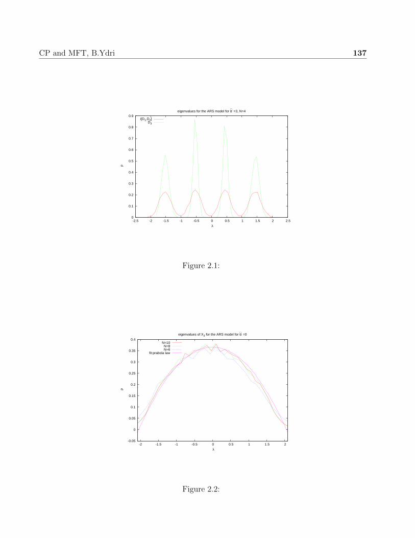
CP and MFT, B.Ydri 137
0
0.1
0.2
0.3
0.4
0.5
0.6
0.7
0.8
0.9
-2.5 -2 -1.5 -1 -0.5 0 0.5 1 1.5 2 2.5
ρ
λ
eigenvalues for the ARS model for α∼ =3, N=4
i[D1,D2]D3
Figure 2.1:
-0.05
0
0.05
0.1
0.15
0.2
0.25
0.3
0.35
0.4
-2 -1.5 -1 -0.5 0 0.5 1 1.5 2
ρ
λ
eigenvalues of X3 for the ARS model for α∼ =0
N=10N=8N=6
fit:prabola law
Figure 2.2:

CP and MFT, B.Ydri 138
0
0.05
0.1
0.15
0.2
0.25
0.3
0.35
0.4
-4 -3 -2 -1 0 1 2 3
ρ
λ
eigenvalues of X3 for the ARS model for N =10
α∼ =0α∼ =0.5
α∼ =1α∼ =1.5
α∼ =2
Figure 2.3:

CP and MFT, B.Ydri 139
-1.5
-1
-0.5
0
0.5
1
1.2 1.4 1.6 1.8 2 2.2 2.4 2.6 2.8 3
<S
>/N
2
α∼
m2= 0 N=16N=24N=32N=48exact
0
1
2
3
4
5
6
-2 0 2 4 6 8 10 12
r
α∼
N=16N=12N=10
theory
0
5
10
15
20
25
30
35
-0.5 0 0.5 1 1.5 2 2.5 3
Tr
Xa2 /N
α∼
N=16N=12N=10
theory
0.6
0.8
1
1.2
1.4
1.6
1.8
2
2.2
0 1 2 3 4 5 6
Cv
α∼
N=16N=24N=32N=48
theory
Figure 2.4:

Bibliography
[1] I. Montvay and G. Munster, “Quantum fields on a lattice,” Cambridge, UK: Univ.
Pr. (1994), 491 p, Cambridge monographs on mathematical physics.
[2] H. J. Rothe, “Lattice gauge theories: An Introduction,” World Sci. Lect. Notes Phys.
74, 1 (2005).
[3] J. Ambjorn, K. N. Anagnostopoulos, W. Bietenholz, T. Hotta and J. Nishimura,
“Large N dynamics of dimensionally reduced 4D SU(N) super Yang-Mills theory,”
JHEP 0007, 013 (2000) [arXiv:hep-th/0003208].
[4] J. Ambjorn, K. N. Anagnostopoulos, W. Bietenholz, T. Hotta and J. Nishimura,
“Monte Carlo studies of the IIB matrix model at large N,” JHEP 0007, 011 (2000)
[arXiv:hep-th/0005147].
[5] K. N. Anagnostopoulos, T. Azuma, K. Nagao and J. Nishimura, “Impact of su-
persymmetry on the nonperturbative dynamics of fuzzy spheres,” JHEP 0509, 046
(2005) [arXiv:hep-th/0506062].
[6] V. G. Filev and D. O’Connor, “On the Phase Structure of Commuting Matrix Mod-
els,” arXiv:1402.2476 [hep-th].
[7] R. Delgadillo-Blando, D. O’Connor and B. Ydri, “Geometry in transition: A model of
emergent geometry,” Phys. Rev. Lett. 100, 201601 (2008) [arXiv:0712.3011 [hep-th]].

Chapter 3
Hybrid Monte Carlo Algorithm
for Noncommutative Phi-Four
3.1 The Matrix Scalar Action
The hybrid Monte Carlo algorithm is a combination of the molecular dynamics method
and the Metropolis algorithm. In this section we will apply this algorithm to matrix Φ4
on the fuzzy sphere. This problem was studied using other techniques in [1–4]. We will
follow here [5, 6].
We are interested in the Euclidean matrix model
S = Tr(− a[La,Φ]2 + bΦ2 + cΦ4
). (3.1)
The scaled (collapsed) parameters are given by
b =b
aN32
, c =c
a2N2. (3.2)
The path integral we wish to sample in Monte Carlo simulation is
Z =
∫dΦ exp(−S[Φ]). (3.3)
As before, we will first think of the configurations Φ as evolving in some fictitious time-like
parameter t, viz
Φ ≡ Φ(t). (3.4)
The above path integral is then equivalent to the Hamiltonian dynamical system
Z =
∫dPdΦ exp(−1
2TrP 2 − S[Φ]). (3.5)
In other words, we have introduced a Hermitian N × N matrix P which is conjugate to
Φ. The Hamiltonian is clearly given by
H =1
2TrP 2 + S[Φ]. (3.6)
CP and MFT, B.Ydri 142
In summary, we think of the matrix Φ as a field in one dimension with corresponding
conjugate momentum P . The Hamiltonian equations of motion read
∂H
∂Pij= (Φ)ij = Pji ,
∂H
∂Φij= −(P )ij =
∂S
∂Φij. (3.7)
We will define the scalar force by
Vij(t) =∂S
∂Φij(t)
= a
(− 4LaΦLa + 2L2
aΦ + 2ΦL2a
)
ji
+ 2bΦji + 4c(Φ3)ji. (3.8)
3.2 The Leap Frog Algorithm
The numerical solution of the above differential equations can be given by the leap
frog equations
(P )ij(t+δt
2) = (P )ij(t)−
δt
2Vij(t). (3.9)
Φij(t+ δt) = Φij(t) + δtPji(t+δt
2). (3.10)
Pij(t+ δt) = Pij(t+δt
2)− δt
2Vij(t+ δt). (3.11)
Let us recall that t = nδt, n = 0, 1, 2, ..., ν− 1, ν where the point n = 0 corresponds to the
initial configuration Φij(0) whereas n = ν corresponds to the final configuration Φij(T )
where T = νδt.
3.3 Hybrid Monte Carlo Algorithm
The hybrid Monte Carlo algorithm can be summarized as follows:
• 1) Choose P (0) such that P (0) is distributed according to the Gaussian probability
distribution exp(−12TrP
2).
• 2)Find the configuration (Φ(T ), P (T )) by solving the above differential equations of
motion.
• 3)Accept the configuration (Φ(T ), P (T )) with a probability
min(1, e−∆H[Φ,P ]), (3.12)
where ∆H is the corresponding change in the Hamiltonian when we go from (Φ(0), P (0))
to (Φ(T ), P (T )).
• 4) Repeat.

CP and MFT, B.Ydri 143
3.4 Optimization
3.4.1 Partial Optimization
We start with some general comment which is not necessarily a part of the optimization
process. The scalar field Φ is a hermitian matrix, i.e. the diagonal elements are real, while
the off diagonal elements are complex conjugate of each other. We find it crucial that we
implement, explicitly in the code, the reality of the diagonal elements by subtracting from
Φii the imaginary part (error) which in each molecular dynamics iteration is small but
can accumulate. The implementation of the other condition is straightforward.
In actual simulations we can fix ν, for example we take ν = 20, and adjust the step size
δt, in some interval [δtmin, δtmax], in such a way that the acceptance rate pa is held fixed
between some target acceptance rates say palow = 70 and pahigh = 90 per cents. If the
acceptance rate becomes larger than the target acceptance rate pahigh, then we increase
the step size δt by a factor inc = 1.2 if the outcome is within the interval [δtmin, δtmax].
Similarly, if the acceptance rate becomes smaller than the target acceptance rate palow,
we decrease the step size by a factor dec = 0.8 if the outcome is within the interval
[δtmin, δtmax]. The adjusting of δt can be done at each Monte Carlo step, but it can also
be performed only each L simulations. We take L = 1. A sample pseudo code is attached
below. A sample of the results is shown in figure (3.1).
pa=(Accept)/(Rejec+Accept)
cou=mod(tmc,L)
if (cou.eq.0)then
if (pa.ge.target_pa_high) then
dtnew=dt*inc
if (dtnew.le.dt_max)then
dt=dtnew
else
dt=dt_max
endif
endif
if (pa.le.target_pa_low) then
dtnew=dt*dec
if (dtnew.ge.dt_min)then
dt=dtnew
else
dt=dt_min
endif
endif
endif
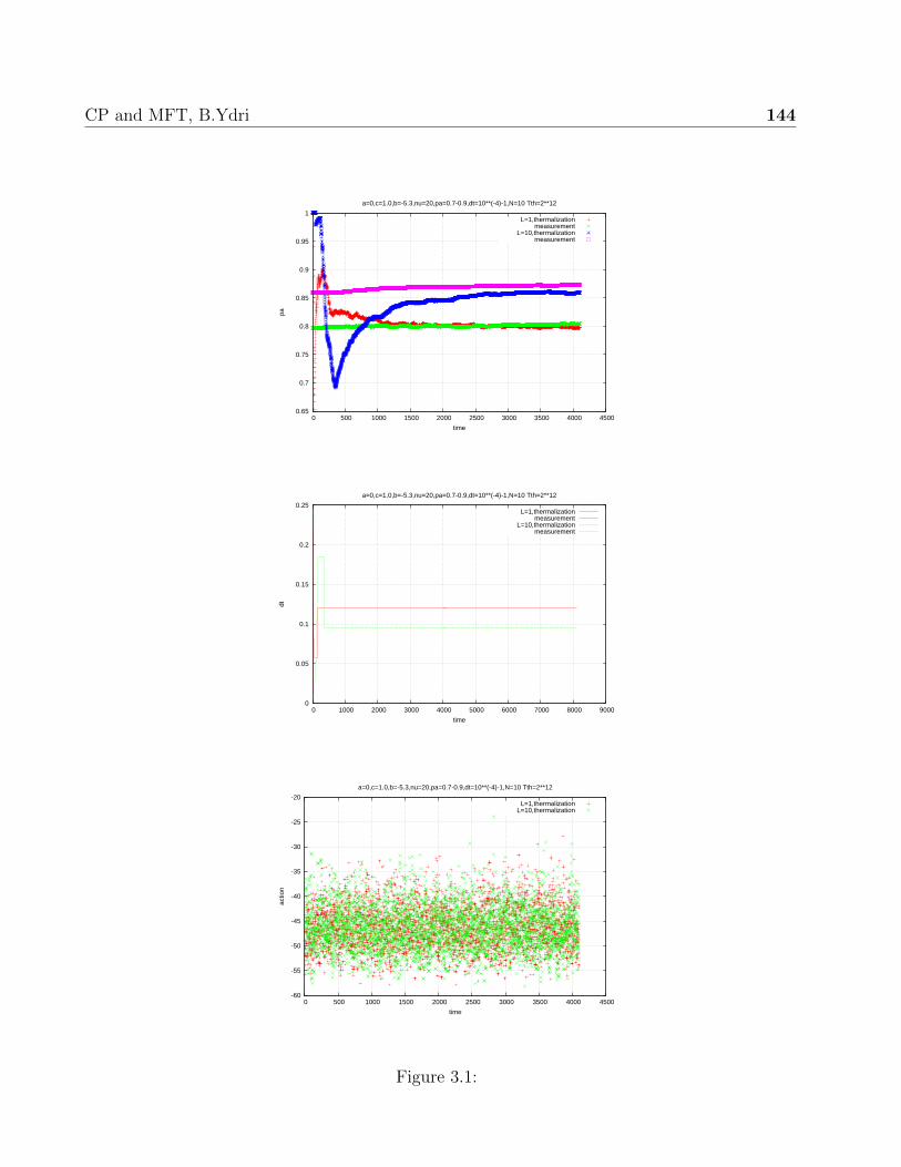
CP and MFT, B.Ydri 144
0.65
0.7
0.75
0.8
0.85
0.9
0.95
1
0 500 1000 1500 2000 2500 3000 3500 4000 4500
pa
time
a=0,c=1.0,b=-5.3,nu=20,pa=0.7-0.9,dt=10**(-4)-1,N=10 Tth=2**12
L=1,thermalizationmeasurement
L=10,thermalizationmeasurement
0
0.05
0.1
0.15
0.2
0.25
0 1000 2000 3000 4000 5000 6000 7000 8000 9000
dt
time
a=0,c=1.0,b=-5.3,nu=20,pa=0.7-0.9,dt=10**(-4)-1,N=10 Tth=2**12
L=1,thermalizationmeasurement
L=10,thermalizationmeasurement
-60
-55
-50
-45
-40
-35
-30
-25
-20
0 500 1000 1500 2000 2500 3000 3500 4000 4500
actio
n
time
a=0,c=1.0,b=-5.3,nu=20,pa=0.7-0.9,dt=10**(-4)-1,N=10 Tth=2**12
L=1,thermalizationL=10,thermalization
Figure 3.1:

CP and MFT, B.Ydri 145
3.4.2 Full Optimization
A more thourough optimization of the algorithm can also be done as follows [1–3].
We take δτ small so that the acceptance rate pa is kept sufficiently large. Then we fix
ν and look for the value of δ × τ where the speed of motion in the phase space defined
by δτ × pa is maximum. Then we fix δτ at its optimal value and look for the value of
ν where the autocorrelation time Tau is minimum. The number of iterations ν must also
be kept relatively small so that the systematic error (which is of order ν × δτ2 for every
hybrid Monte Carlo unit of time) is kept small. Clearly a small value of ν is better for
the effeciency of the algorithm.
3.5 The Non-Uniform Order: Another Exotic Phase
3.5.1 Phase Structure
The theory (3.1) is a three-parameter model with the following three known phases:
• The usual 2nd order Ising phase transition between disordered < Φ >= 0 and
uniform ordered < Φ >∼ 1 phases. This appears for small values of c. This is the
only transition observed in commutative phi-four.
• A matrix transition between disordered < Φ >= 0 and non-uniform ordered < Φ >∼γ phases with γ2 = 1. This transition coincides, for very large values of c, with the
3rd order transition of the real quartic matrix model, i.e. the model with a = 0,
which occurs at b = −2√Nc. See next chapter.
• A transition between uniform ordered < Φ >∼ 1 and non-uniform ordered < Φ >∼γ phases. The non-uniform phase, in which translational/rotational invariance is
spontaneously broken, is absent in the commutative theory. The non-uniform phase
is essentially the stripe phase observed originally on Moyal-Weyl spaces in [7, 8].
The above three phases are already present in the pure potential model V = Tr(bΦ2+cΦ4).
The ground state configurations are given by the matrices
Φ0 = 0. (3.13)
Φγ =
√− b
2cUγU+ , γ2 = 1N , UU+ = U+U = 1N . (3.14)
We compute V [Φ0] = 0 and V [Φγ ] = −b2/4c. The first configuration corresponds to
the disordered phase characterized by < Φ >= 0. The second solution makes sense
only for b < 0, and it corresponds to the ordered phase characterized by < Φ >6= 0.
As mentioned above, there is a non-perturbative transition between the two phases which
occurs quantum mechanically, not at b = 0, but at b = b∗ = −2√Nc, which is known as the
one-cut to two-cut transition. The idempotent γ can always be chosen such that γ = γk =
diag(1k,−1N−k). The orbit of γk is the Grassmannian manifold U(N)/(U(k)×U(N−k))
which is dk−dimensional where dk = 2kN − 2k2. It is not difficult to show that this

CP and MFT, B.Ydri 146
dimension is maximum at k = N/2, assuming that N is even, and hence from entropy
argument, the most important two-cut solution is the so-called stripe configuration given
by γ = diag(1N/2,−1N/2).
In this real quartic matrix model, we have therefore three possible phases characterized
by the following order parameters:
< Φ >= 0 disordered phase. (3.15)
< Φ >= ±√− b
2c1N Ising (uniform) phase. (3.16)
< Φ >= ±√− b
2cγ matrix (nonuniform or stripe) phase. (3.17)
However, as one can explicitly check by calculating the free energies of the respective
phases, the uniform ordered phase is not stable in the real quartic matrix model V =
Tr(bΦ2 + cΦ4).
The above picture is expected to hold for noncommutative/fuzzy phi-four theory in any
dimension, and the three phases are all stable and are expected to meet at a triple point.
This structure was confirmed in two dimensions by means of Monte Carlo simulations on
the fuzzy sphere in [1, 2].
3.5.2 Sample Simulations
We run simulations for every N by running Tth thermalization steps, and then mea-
suring observables in a sample containing Tmc thermalized configurations Φ, where each
two successive configurations are separated by Tco Monte Carlo steps in order to reduce
auto-correlation effects. Most of the detail of the simulations have already been explained.
We only mention again that we estimate error bars using the jackknife method and use
the random number generator ran2. A sample code is attached in the last chapter.
We measure the action < S >, the specific heat Cv, the magnetization m and the
associated susceptibility χ, the total power PT , and the power in the zero modes P0
defined respectively by
Cv =< S2 > − < S >2 . (3.18)
m =< |TrΦ| > . (3.19)
χ =< |TrΦ|2 > − < |TrΦ| >2 . (3.20)
PT =1
NTrΦ2. (3.21)
P0 =1
N2(TrΦ)2. (3.22)
We will also compute the eigenvalues of the matrix Φ by calling the library LAPACK and
then construct appropriate histograms using known techniques.
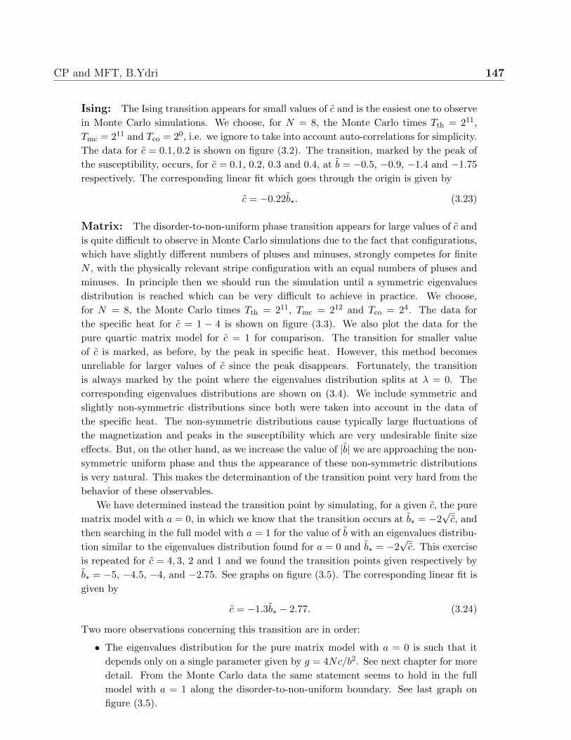
CP and MFT, B.Ydri 147
Ising: The Ising transition appears for small values of c and is the easiest one to observe
in Monte Carlo simulations. We choose, for N = 8, the Monte Carlo times Tth = 211,
Tmc = 211 and Tco = 20, i.e. we ignore to take into account auto-correlations for simplicity.
The data for c = 0.1, 0.2 is shown on figure (3.2). The transition, marked by the peak of
the susceptibility, occurs, for c = 0.1, 0.2, 0.3 and 0.4, at b = −0.5, −0.9, −1.4 and −1.75
respectively. The corresponding linear fit which goes through the origin is given by
c = −0.22b∗. (3.23)
Matrix: The disorder-to-non-uniform phase transition appears for large values of c and
is quite difficult to observe in Monte Carlo simulations due to the fact that configurations,
which have slightly different numbers of pluses and minuses, strongly competes for finite
N , with the physically relevant stripe configuration with an equal numbers of pluses and
minuses. In principle then we should run the simulation until a symmetric eigenvalues
distribution is reached which can be very difficult to achieve in practice. We choose,
for N = 8, the Monte Carlo times Tth = 211, Tmc = 212 and Tco = 24. The data for
the specific heat for c = 1 − 4 is shown on figure (3.3). We also plot the data for the
pure quartic matrix model for c = 1 for comparison. The transition for smaller value
of c is marked, as before, by the peak in specific heat. However, this method becomes
unreliable for larger values of c since the peak disappears. Fortunately, the transition
is always marked by the point where the eigenvalues distribution splits at λ = 0. The
corresponding eigenvalues distributions are shown on (3.4). We include symmetric and
slightly non-symmetric distributions since both were taken into account in the data of
the specific heat. The non-symmetric distributions cause typically large fluctuations of
the magnetization and peaks in the susceptibility which are very undesirable finite size
effects. But, on the other hand, as we increase the value of |b| we are approaching the non-
symmetric uniform phase and thus the appearance of these non-symmetric distributions
is very natural. This makes the determinantion of the transition point very hard from the
behavior of these observables.
We have determined instead the transition point by simulating, for a given c, the pure
matrix model with a = 0, in which we know that the transition occurs at b∗ = −2√c, and
then searching in the full model with a = 1 for the value of b with an eigenvalues distribu-
tion similar to the eigenvalues distribution found for a = 0 and b∗ = −2√c. This exercise
is repeated for c = 4, 3, 2 and 1 and we found the transition points given respectively by
b∗ = −5, −4.5, −4, and −2.75. See graphs on figure (3.5). The corresponding linear fit is
given by
c = −1.3b∗ − 2.77. (3.24)
Two more observations concerning this transition are in order:
• The eigenvalues distribution for the pure matrix model with a = 0 is such that it
depends only on a single parameter given by g = 4Nc/b2. See next chapter for more
detail. From the Monte Carlo data the same statement seems to hold in the full
model with a = 1 along the disorder-to-non-uniform boundary. See last graph on
figure (3.5).

CP and MFT, B.Ydri 148
• The disorder-to-non-uniform transition line seems to be better approximated by a
shift of the result b∗ = −2√c by a single unit in the −b direction. This is roughly in
accord with the analytic result for the critical point found in [9] for the multitrace
approximation (see next chapter) which is given, for a = 1, by
b∗ = −√N
2− 2√c+
N
6√c. (3.25)
Stripe: The uniform-to-non-uniform phase transition is even more difficult to observe
in Monte Carlo simulations but it is expected, according to [1,2], to only be a continuation
of the disorder-to-uniform transition line (3.23). The intersection point between the above
two fits (3.23) and (3.24) is therefore an estimation of the triple point. This is given by
(c, b) = (0.56,−2.57). (3.26)
However, this is not really what we observe using our code here. The uniform-to-non-
uniform phase transition is only observed for small values of c from the uniform phase to
the non-uniform phase as we increase −b. The transition for these small values of c, such
as c = 0.1, 0.2, 0.3, 0.4, corresponds to a second peak in the susceptibility and the specific
heat. It corresponds to a transition from a one-cut eigenvalues distribution symmetric
around 0 to a one-cut eigenvalues distribution symmetric around a non-zero value. The
eigenvalues distributions for c = 0.3 are shown on the first two graphs of figure (3.7).
In this case we have found it much easier to determine the transition points from the
behavior of the magnetization and the powers. In particular, we have determined the
transition point from the broad maximum of the magnetization which corresponds to the
discontinuity of the power in the zero modes. The magnetization and the powers, for
c = 0.1, 0.2, 0.3, 0.4, are shown on figure (3.8). The transition points were found to be
−1.5, −1.7, −2 and −2.1 respectively.
The uniform phase becomes narrower as we approach the value c = 0.5. The specific
heat and the susceptibility have a peak around b = −2.25 which is consistent with the
Ising transition but the powers and the magnetization show the behavior of the disorder-
to-non-uniform-order transition. The eigenvalues distribution is also consistent with the
disorder-to-non-uniform-order transition. See last graph of figure (3.7). The value c = 0.5
is roughly the location of the triple point.
The phase diagram is shown on figure (3.6).

CP and MFT, B.Ydri 149
0
0.2
0.4
0.6
0.8
1
1.2
1.4
1.6
1.8
-1.4 -1.2 -1 -0.8 -0.6 -0.4 -0.2 0
PT,P
0
bT
N=8
cT=0.1,PTP0
cT=0.2,PTP0
0
1
2
3
4
5
6
7
8
9
10
11
-1.4 -1.2 -1 -0.8 -0.6 -0.4 -0.2 0
m
bT
N=8
cT=0.1cT=0.2
0
0.5
1
1.5
2
2.5
3
3.5
4
4.5
-1.4 -1.2 -1 -0.8 -0.6 -0.4 -0.2 0
χ
bT
N=8
cT=0.1cT=0.2
Figure 3.2:

CP and MFT, B.Ydri 150
0.2
0.3
0.4
0.5
0.6
0.7
0.8
-10 -9 -8 -7 -6 -5 -4 -3 -2 -1 0
Cv/
N2
bT
N=8
a=1.0,cT=1.0cT=2.0cT=3.0cT=4.0
0.1
0.2
0.3
0.4
0.5
0.6
0.7
0.8
-6 -5 -4 -3 -2 -1 0
Cv/
N2
bT
N=8
a=1.0,cT=1.0a=0,cT=1.0
0
0.05
0.1
0.15
0.2
0.25
0.3
0.35
0.4
0.45
-3 -2.5 -2 -1.5 -1 -0.5 0
PT,P
0
bT
N=8
a=1.0,cT=1.0,PTP0
0
0.1
0.2
0.3
0.4
0.5
0.6
-3 -2.5 -2 -1.5 -1 -0.5 0
PT,P
0
bT
N=8
a=0.0,cT=1.0,PTP0
0.1
0.2
0.3
0.4
0.5
0.6
0.7
0.8
0.9
1
-4 -3.5 -3 -2.5 -2 -1.5 -1 -0.5 0
m
bT
N=8
a=1.0,cT=1.0
0.16
0.18
0.2
0.22
0.24
0.26
0.28
0.3
0.32
-3 -2.5 -2 -1.5 -1 -0.5 0
m
bT
N=8
a=0.0,cT=1.0
0
0.05
0.1
0.15
0.2
0.25
0.3
0.35
-4 -3.5 -3 -2.5 -2 -1.5 -1 -0.5 0
χ
bT
N=8
a=1.0,cT=1.0
0.005
0.01
0.015
0.02
0.025
0.03
0.035
-3 -2.5 -2 -1.5 -1 -0.5 0
m
bT
N=8
a=0.0,cT=1.0
Figure 3.3:

CP and MFT, B.Ydri 151
0
0.2
0.4
0.6
0.8
1
1.2
1.4
1.6
1.8
2
-0.8 -0.6 -0.4 -0.2 0 0.2 0.4 0.6 0.8
ρ (λ
)
λ
N=8
cT=4.0, bT=-1.5bT=-5.0bT=-5.5bT=-6.0
0
0.5
1
1.5
2
2.5
-0.8 -0.6 -0.4 -0.2 0 0.2 0.4 0.6 0.8 1
ρ (λ
)
λ
N=8
cT=4.0, bT=-6.1bT=-6.5bT=-6.9bT=-7.5bT=-9.5
0
0.5
1
1.5
2
2.5
3
-1 -0.8 -0.6 -0.4 -0.2 0 0.2 0.4 0.6 0.8
ρ (λ
)
λ
N=8
cT=4.0, bT=-7.0bT=-8.0bT=-9.0
bT=-10.0
Figure 3.4:
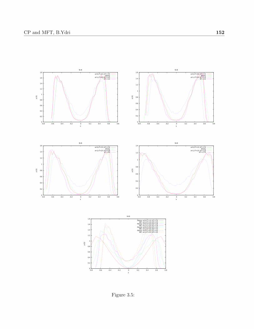
CP and MFT, B.Ydri 152
0
0.2
0.4
0.6
0.8
1
1.2
1.4
1.6
1.8
-0.8 -0.6 -0.4 -0.2 0 0.2 0.4 0.6 0.8
ρ (λ
)
λ
N=8
a=0,cT=4.0, bT=-4.0theory
a=1,cT=4.0, bT=-4.0bT=-5.0
0
0.2
0.4
0.6
0.8
1
1.2
1.4
1.6
-0.8 -0.6 -0.4 -0.2 0 0.2 0.4 0.6 0.8
ρ (λ
)
λ
N=8
a=0,cT=3.0, bT=-3.4theory
a=1,cT=3.0, bT=-3.4bT=-4.5
0
0.2
0.4
0.6
0.8
1
1.2
1.4
1.6
-0.8 -0.6 -0.4 -0.2 0 0.2 0.4 0.6 0.8
ρ (λ
)
λ
N=8
a=0,cT=2.0, bT=-2.8theory
a=1,cT=2.0, bT=-2.8bT=-4.0
0
0.2
0.4
0.6
0.8
1
1.2
1.4
-0.8 -0.6 -0.4 -0.2 0 0.2 0.4 0.6 0.8
ρ (λ
)
λ
N=8
a=0,cT=1.0, bT=-2.0theory
a=1,cT=1.0, bT=-2.0bT=-2.75
0
0.2
0.4
0.6
0.8
1
1.2
1.4
1.6
1.8
-0.8 -0.6 -0.4 -0.2 0 0.2 0.4 0.6 0.8
ρ (λ
)
λ
N=8
theory: a=0,cT=1.0, bT=-2.0MC: a=1,cT=1.0, bT=-2.0
theory: a=0,cT=2.0, bT=-2.8MC: a=1,cT=2.0, bT=-2.8
theory: a=0,cT=3.0, bT=-3.4MC: a=1,cT=3.0, bT=-3.4
theory: a=0,cT=4.0, bT=-4.0MC: a=1,cT=4.0, bT=-4.0
Figure 3.5:
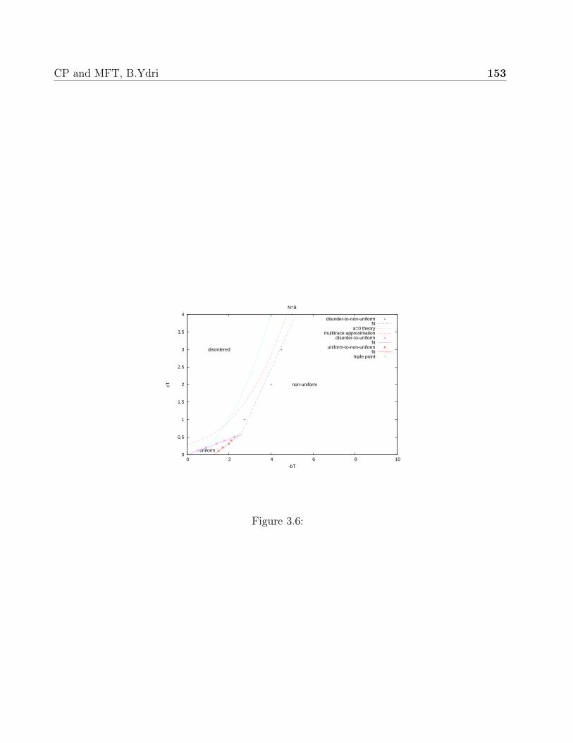
CP and MFT, B.Ydri 153
0
0.5
1
1.5
2
2.5
3
3.5
4
0 2 4 6 8 10
cT
-bT
N=8
disordered
non-uniform
uniform
disorder-to-non-uniformfit
a=0 theorymultitrace approximation
disorder-to-uniformfit
uniform-to-non-uniformfit
triple point
Figure 3.6:

CP and MFT, B.Ydri 154
0
0.2
0.4
0.6
0.8
1
1.2
1.4
1.6
1.8
-1.5 -1 -0.5 0 0.5 1 1.5
ρ (λ
)
λ
N=8
cT=0.3, bT=-0.25bT=-1.0
bT=-1.25bT=-1.5
bT=-1.75
0
0.2
0.4
0.6
0.8
1
1.2
1.4
1.6
1.8
-1.5 -1 -0.5 0 0.5 1 1.5 2
ρ (λ
)
λ
N=8
cT=0.3, bT=-2.0bT=-2.25
bT=-2.5bT=-3.0
0
0.5
1
1.5
2
2.5
-2 -1.5 -1 -0.5 0 0.5 1 1.5 2
ρ (λ
)
λ
N=8
cT=0.5, bT=-2.0bT=-2.25 bT=-3.0bT=-7.0
Figure 3.7:

CP and MFT, B.Ydri 155
0
0.2
0.4
0.6
0.8
1
1.2
1.4
1.6
1.8
2
-3.5 -3 -2.5 -2 -1.5 -1 -0.5 0 0.5
PT,P
0
bT
N=8
cT=0.2,PTP0
cT=0.3,PTP0
cT=0.4,PTP0
0
1
2
3
4
5
6
7
8
9
10
-3.5 -3 -2.5 -2 -1.5 -1 -0.5 0 0.5
m
bT
N=8
cT=0.2cT=0.3cT=0.4
Figure 3.8:
Bibliography
[1] F. Garcia Flores, X. Martin and D. O’Connor, “Simulation of a scalar field on a fuzzy
sphere,” Int. J. Mod. Phys. A 24, 3917 (2009) [arXiv:0903.1986 [hep-lat]].
[2] F. Garcia Flores, D. O’Connor and X. Martin, “Simulating the scalar field on the
fuzzy sphere,” PoS LAT 2005, 262 (2006) [hep-lat/0601012].
[3] X. Martin, “A matrix phase for the phi**4 scalar field on the fuzzy sphere,” JHEP
0404, 077 (2004) [hep-th/0402230].
[4] M. Panero, “Numerical simulations of a non-commutative theory: The Scalar model
on the fuzzy sphere,” JHEP 0705, 082 (2007) [hep-th/0608202].
[5] J. Ambjorn, K. N. Anagnostopoulos, W. Bietenholz, T. Hotta and J. Nishimura,
“Large N dynamics of dimensionally reduced 4D SU(N) super Yang-Mills theory,”
JHEP 0007, 013 (2000) [arXiv:hep-th/0003208].
[6] J. Ambjorn, K. N. Anagnostopoulos, W. Bietenholz, T. Hotta and J. Nishimura,
“Monte Carlo studies of the IIB matrix model at large N,” JHEP 0007, 011 (2000)
[arXiv:hep-th/0005147].
[7] S. S. Gubser and S. L. Sondhi, “Phase structure of noncommutative scalar field
theories,” Nucl. Phys. B 605, 395 (2001) [hep-th/0006119].
[8] J. Ambjorn and S. Catterall, “Stripes from (noncommutative) stars,” Phys. Lett. B
549, 253 (2002) [hep-lat/0209106].
[9] B. Ydri, “A Multitrace Approach to Noncommutative Φ42,” arXiv:1410.4881 [hep-th].

Chapter 4
Lattice HMC Simulations of Φ42: A
Lattice Example
References for this chapter include the elegant quantum field theory textbook [1] and
the original articles [2–4].
4.1 Model and Phase Structure
The Euclidean φ4 action with O(N) symmetry is given by
S[φ] =
∫ddx
(1
2(∂µφ
i)2 +1
2m2φiφi +
λ
4(φiφi)2
). (4.1)
We will employ lattice regularization in which x = an,∫ddx = ad
∑n, φi(x) = φin and
∂µφi = (φin+µ − φin)/a. The lattice action reads
S[φ] =∑
n
(− 2κ
∑
µ
ΦinΦi
n+µ + ΦinΦi
n + g(ΦinΦi
n − 1)2
). (4.2)
The mass parameter m2 is replaced by the so-called hopping parameter κ and the coupling
constant λ is replaced by the coupling constant g where
m2a2 =1− 2g
κ− 2d ,
λ
ad−4=
g
κ2. (4.3)
The fields φin and Φin are related by
φin =
√2κ
ad−2Φin. (4.4)
The partition function is given by
Z =
∫ ∏
n,i
dΦin e−S[φ]
=
∫dµ(Φ) e2κ
∑n
∑µ ΦinΦin+µ . (4.5)
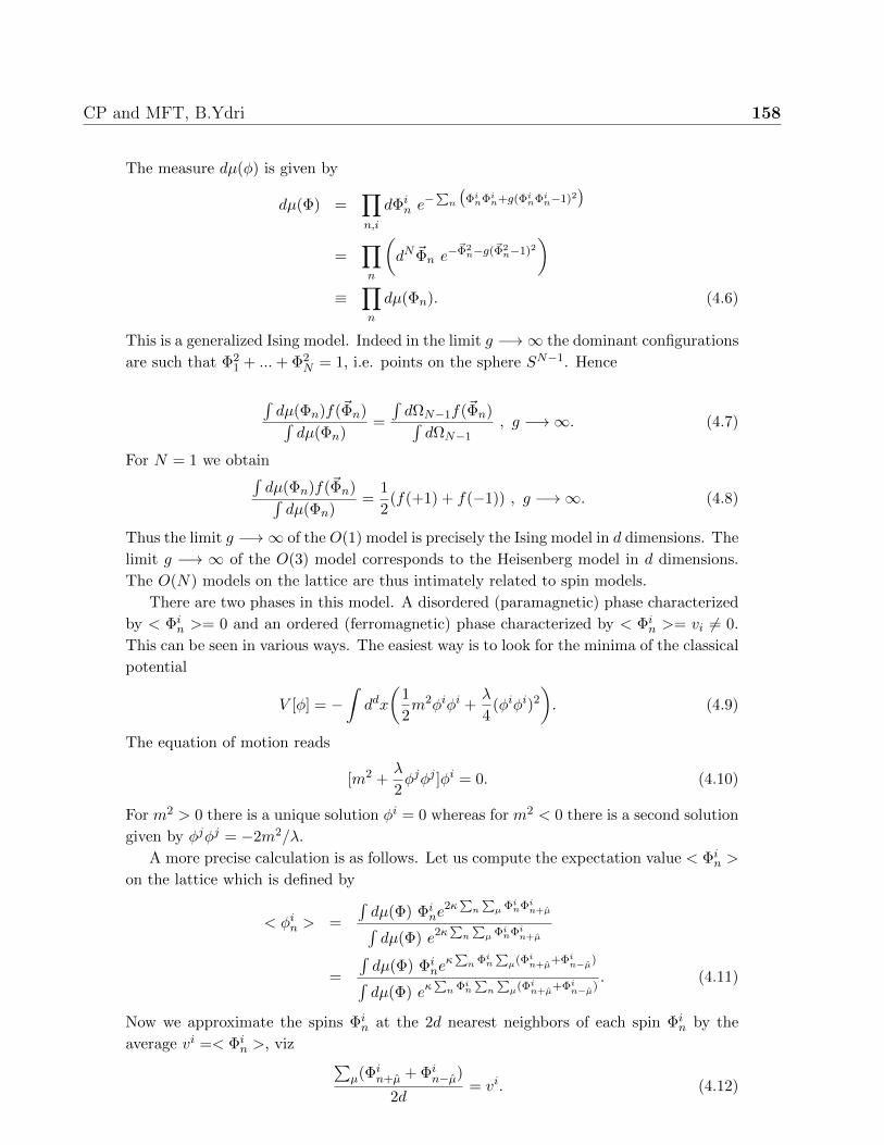
CP and MFT, B.Ydri 158
The measure dµ(φ) is given by
dµ(Φ) =∏
n,i
dΦin e−∑
n
(ΦinΦin+g(ΦinΦin−1)2
)
=∏
n
(dN ~Φn e
−~Φ2n−g(~Φ2
n−1)2
)
≡∏
n
dµ(Φn). (4.6)
This is a generalized Ising model. Indeed in the limit g −→∞ the dominant configurations
are such that Φ21 + ...+ Φ2
N = 1, i.e. points on the sphere SN−1. Hence
∫dµ(Φn)f(~Φn)∫
dµ(Φn)=
∫dΩN−1f(~Φn)∫
dΩN−1, g −→∞. (4.7)
For N = 1 we obtain∫dµ(Φn)f(~Φn)∫
dµ(Φn)=
1
2(f(+1) + f(−1)) , g −→∞. (4.8)
Thus the limit g −→∞ of the O(1) model is precisely the Ising model in d dimensions. The
limit g −→ ∞ of the O(3) model corresponds to the Heisenberg model in d dimensions.
The O(N) models on the lattice are thus intimately related to spin models.
There are two phases in this model. A disordered (paramagnetic) phase characterized
by < Φin >= 0 and an ordered (ferromagnetic) phase characterized by < Φi
n >= vi 6= 0.
This can be seen in various ways. The easiest way is to look for the minima of the classical
potential
V [φ] = −∫ddx
(1
2m2φiφi +
λ
4(φiφi)2
). (4.9)
The equation of motion reads
[m2 +λ
2φjφj ]φi = 0. (4.10)
For m2 > 0 there is a unique solution φi = 0 whereas for m2 < 0 there is a second solution
given by φjφj = −2m2/λ.
A more precise calculation is as follows. Let us compute the expectation value < Φin >
on the lattice which is defined by
< φin > =
∫dµ(Φ) Φi
ne2κ
∑n
∑µ ΦinΦin+µ
∫dµ(Φ) e2κ
∑n
∑µ ΦinΦin+µ
=
∫dµ(Φ) Φi
neκ∑n Φin
∑µ(Φin+µ+Φin−µ)
∫dµ(Φ) eκ
∑n Φin
∑n
∑µ(Φin+µ+Φin−µ)
. (4.11)
Now we approximate the spins Φin at the 2d nearest neighbors of each spin Φi
n by the
average vi =< Φin >, viz
∑µ(Φi
n+µ + Φin−µ)
2d= vi. (4.12)

CP and MFT, B.Ydri 159
This is a crude form of the mean field approximation. Equation (4.11) becomes
vi =
∫dµ(Φ) Φi
ne4κd
∑n Φinv
i
∫dµ(Φ) e4κd
∑n Φinv
i
=
∫dµ(Φn) Φi
ne4κdΦinv
i
∫dµ(Φi
n) e4κdΦinvi . (4.13)
The extra factor of 2 in the exponents comes from the fact that the coupling between any
two nearest neighbor spins on the lattice occurs twice. We write the above equation as
vi =∂
∂J ilnZ[J ]|Ji=4κdvi . (4.14)
Z[J ] =
∫dµ(Φn) eΦinJ
i
=
∫dNΦi
n e−ΦinΦin−g(ΦinΦin−1)2+ΦinJ
i. (4.15)
The limit g −→ 0: In this case we have
Z[J ] =
∫dNΦi
n e−ΦinΦin+ΦinJ
i= Z[0] e
JiJi
4 . (4.16)
In other words
vi = 2κcdvi ⇒ κc =
1
2d. (4.17)
The limit g −→∞: In this case we have
Z[J ] = N∫dNΦi
n δ(ΦinΦi
n − 1) eΦinJi
= N∫dNΦi
n δ(ΦinΦi
n − 1)
[1 + Φi
nJi +
1
2ΦinΦj
nJiJ j + ...
]. (4.18)
By using rotational invariance in N dimensions we obtain∫dNΦi
n δ(ΦinΦi
n − 1) Φin = 0. (4.19)
∫dNΦi
n δ(ΦinΦi
n − 1) ΦinΦj
n =δij
N
∫dNΦi
n δ(ΦinΦi
n − 1) ΦknΦk
n =δij
N
Z[0]
N . (4.20)
Hence
Z[J ] = Z[0]
[1 +
J iJ i
2N+ ...
]. (4.21)
Thus
vi =J i
N=
4κcdvi
N⇒ κc =
N
4d. (4.22)

CP and MFT, B.Ydri 160
The limit of The Ising Model: In this case we have
N = 1 , g −→∞. (4.23)
We compute then
Z[J ] = N∫dΦn δ(Φ
2n − 1) eΦnJ
= Z[0] coshJ. (4.24)
Thus
v = tanh 4κdv. (4.25)
A graphical sketch of the solutions of this equation will show that for κ < κc there is only
one intersection point at v = 0 whereas for κ > κc there are two intersection points away
from the zero, i.e. v 6= 0. Clearly for κ near κc the solution v is near 0 and thus we can
expand the above equation as
v = 4κdv − 1
3(4κd)3v2 + .... (4.26)
The solution is
1
3(4d)2κ3v2 = κ− κc. (4.27)
Thus only for κ > κc there is a non zero solution.
In summary we have the two phases
κ > κc : broken, ordered, ferromagnetic (4.28)
κ < κc : symmetric,disordered, paramagnetic. (4.29)
The critical line κc = κc(g) interpolates in the κ− g plane between the two lines given by
κc =N
4d, g −→∞. (4.30)
κc =1
2d, g −→ 0. (4.31)
For d = 4 the critical value at g = 0 is κc = 1/8 for all N . This critical value can be
derived in a different way as follows. We know that the renormalized mass at one-loop
order in the continuum φ4 with O(N) symmetry is given by the equation
m2R = m2 + (N + 2)λI(m2,Λ)
= m2 +(N + 2)λ
16π2Λ2 +
(N + 2)λ
16π2m2 ln
m2
Λ2+
(N + 2)λ
16π2m2C + finite terms.
(4.32)

CP and MFT, B.Ydri 161
This equation reads in terms of dimensionless quantities as follows
a2m2R = am2 +
(N + 2)λ
16π2+
(N + 2)λ
16π2a2m2 ln a2m2 +
(N + 2)λ
16π2a2m2C + a2 × finite terms.
(4.33)
The lattice space a is formally identified with the inverse cut off 1/Λ, viz
a =1
Λ. (4.34)
Thus we obtain in the continuum limit a −→ 0 the result
a2m2 −→ −(N + 2)λ
16π2+
(N + 2)λ
16π2a2m2 ln a2m2 +
(N + 2)λ
16π2a2m2C + a2 × finite terms.
(4.35)
In other words (with r0 = (N + 2)/8π2)
a2m2 −→ a2m2c = −r0
2λ+O(λ2). (4.36)
This is the critical line for small values of the coupling constant as we will now show.
Expressing this equation in terms of κ and g we obtain
1− 2g
κ− 8 −→ −r0
2
g
κ2+O(λ2). (4.37)
This can be brought to the form
[κ− 1
16(1− 2g)
]2
−→ 1
256
[1 + 16r0g − 4g
]+O(g2/κ2). (4.38)
We get the result
κ −→ κc =1
8+ (
r0
2− 1
4)g +O(g2). (4.39)
This result is of fundamental importance. The continuum limit a −→ 0 corresponds
precisely to the limit in which the mass approaches its critical value. This happens for
every value of the coupling constant and hence the continuum limit a −→ 0 is the limit
in which we approach the critical line. The continuum limit is therefore a second order
phase transition.
4.2 The HM Algorithm
We start by considering the Hamiltonian
H[φ, P ] =1
2
∑
n
P inPin +
∑
n
(− 2κ
∑
µ
ΦinΦi
n+µ + ΦinΦi
n + g(ΦinΦi
n − 1)2
).(4.40)

CP and MFT, B.Ydri 162
The Hamilton equations of motion are
∂H
∂P in= Φi
n = P in
∂H
∂Φin
= −P in = V in. (4.41)
The force is given by
V in =
∂S
∂Φin
= −2κ∑
µ
(Φin+µ + Φi
n−µ) + 2Φin + 4gΦi
n(ΦjnΦj
n − 1). (4.42)
The leap frog, or Stormer-Verlet, algorithm, which maintains the symmetry under time
reversible and the conservation of the phase space volume of the above Hamilton equations,
is then given by the equations
P in(t+δt
2) = (P )in(t)− δt
2V in(t). (4.43)
Φin(t+ δt) = Φi
n(t) + δtP in(t+δt
2). (4.44)
P in(t+ δt) = P in(t+δt
2)− δt
2V in(t+ δt). (4.45)
We recall that t = nδt, n = 0, 1, 2, ..., ν − 1, ν where the point n = 0 corresponds to the
initial configuration Φin(0) whereas n = ν corresponds to the final configuration Φi
n(T )
where T = νδt. This algorithm does not conserve the Hamiltonian due to the systematic
error associated with the discretization, which goes as O(δt2), but as can be shown the
addition of a Metropolis accept-reject step will nevertheless lead to an exact algorithm.
The hybrid Monte Carlo algorithm in this case can be summarized as follows:
• 1) Choose P (0) such that P (0) is distributed according to the Gaussian probability
distribution exp(−12
∑n P
inP
in). In particular we choose P in such that
P in =√−2 ln(1− x1) cos 2π(1− x2), (4.46)
where x1 and x2 are two random numbers uniformly distributed in the interval [0, 1].
This step is crucial if we want to avoid ergodic problems.
• 2)Find the configuration (Φ(T ), P (T )) by solving the above differential equations of
motion.
• 3)Accept the configuration (Φ(T ), P (T )) with a probability
min(1, e−∆H[Φ,P ]), (4.47)
where ∆H is the corresponding change in the Hamiltonian when we go from (Φ(0), P (0))
to (Φ(T ), P (T )).
• 4) Repeat.

CP and MFT, B.Ydri 163
4.3 Renormalization and Continuum Limit
The continuum and lattice actions for Φ4 theory in two dimensions with N = 1 are
given, with some slight change of notation, by
S[φ] =
∫d2x
(1
2(∂µφ)2 +
1
2µ2
0φ2 +
λ
4φ4
). (4.48)
S[φ] =∑
n
(− 2κ
∑
µ
ΦnΦn+µ + Φ2n + g(Φ2
n − 1)2
). (4.49)
µ20 = m2. (4.50)
µ20l ≡ µ2
0a2 =
1− 2g
κ− 4 , λl ≡ λa2 =
g
κ2. (4.51)
In the simulations we will start by fixing the lattice quartic coupling λl and the lattice
mass parameter µ20l which then allows us to fix κ and g as
κ =
√8λl + (µ2
0l + 4)2 − (µ20l + 4)
4λl. (4.52)
g = κ2λl. (4.53)
The phase diagram will be drawn originally in the µ20l−λl plane. This is the lattice phase
diagram. This should be extrapolated to the infinite volume limit L = Na −→∞.
The Euclidean quantum field theory phase diagram should be drawn in terms of the
renormalized parameters and is obtained from the lattice phase diagram by taking the limit
a −→ 0. In two dimensions the Φ4 theory requires only mass renormalization while the
quartic coupling constant is finite. Indeed, the bare mass µ20 diverges logarithmically when
we remove the cutoff, i.e. in the limit Λ −→ ∞ where Λ = 1/a while λ is independent of
a. As a consequence, the lattice parameters will go to zero in the continuum limit a −→ 0.
We know that mass renormalization is due to the tadpole diagram which is the only
divergent Feynman diagram in the theory and takes the form of a simple reparametrization
given by
µ20 = µ2 − δµ2, (4.54)
where µ2 is the renormalized mass parameter and δµ2 is the counter term which is fixed
via an appropriate renormalization condition. The unltraviolet divergence ln Λ of µ20
is contained in δµ2 while the renormalization condition will split the finite part of µ20
between µ2 and δµ2. The choice of the renormalization condition can be quite arbitrary. A
convenient choice suitable for Monte Carlo measurements and which distinguishes between
the two phases of the theory is given by the usual normal ordering prescription [2] .

CP and MFT, B.Ydri 164
Quantization at one-loop gives explicitly the 2−point function
Γ(2)(p) = p2 + µ20 + 3λ
∫d2k
(2π)2
1
k2 + µ20
. (4.55)
A self-consistent Hartree treatment gives then the result
Γ(2)(p) = p2 + µ20 + 3λ
∫d2k
(2π)2
1
Γ(2)(k)
= p2 + µ2 + 3λ
∫d2k
(2π)2
1
Γ(2)(k)− δµ2
= p2 + µ2 + 3λ
∫d2k
(2π)2
1
k2 + µ2− δµ2 + two− loop
(4.56)
This should certainly work in the symmetric phase where µ2 > 0. We can also write this
as
Γ(2)(p) = p2 + µ2 + Σ(p) , Σ(p) = 3λAµ2 − δµ2 + two− loop. (4.57)
Aµ2 is precisely the value of the tadpole diagram given by
Aµ2 =
∫d2k
(2π)2
1
k2 + µ2. (4.58)
The renormalization condition which is equivalent to normal ordering the interaction in
the interaction picture in the symmetric phase is equivalent to the choice
δµ2 = 3λAµ2 . (4.59)
A dimensionless coupling constant can the be defined by
f =λ
µ2. (4.60)
The action becomes
S[φ] =
∫d2x
(1
2(∂µφ)2 +
1
2µ2(1− 3fAµ2)φ2 +
fµ2
4φ4
). (4.61)
For sufficiently small f the exact effective potential is well approximated by the classical
potential with a single minimum at φcl = 0. For larger f , the coefficient of the mass term
in the above action can become negative and as a consequence a transition to the broken
symmetry phase is possible, although in this regime the effective potential is no longer
well approximated by the classical potential. Indeed, a transition to the broken symmetry
phase was shown to be present in [4], where a duality between the strong coupling regime
of the above action and a weakly coupled theory normal ordered with respect to the broken
phase was explicitly constructed.
The sites on the lattice are located at xµ = nµa where nµ = 0, ..., N − 1 with L = Na.
The plane waves on a finite volume lattice with periodic boundary conditions are exp(ipx)
CP and MFT, B.Ydri 165
with pµ = mµ2π/L where mµ = −N/2+1,−N/2+2, ..., N/2 for N even. This means that
the zero of the x−space is located at the edge of the box while the zero of the p−space
is located in the middle of the box. We have therefore the normalization conditions∑x exp(−i(p − p′)x) = δp,p′ and
∑p exp(−i(x − x′)p) = δx,x′ where, for example,
∑p =∑
m /L2. In the infinite volume limit defined by L = Na −→ ∞ with a fixed we have∑
p −→∫ π/a−π/a d
2p/(2π)2. It is not difficult to show that on the lattice the propagator
1/(p2 + µ2) becomes a2/(4∑
µ sin2 apµ/2 + µ2l ) [1]. Thus on a finite volume lattice with
periodic boundary conditions the Feynman diagram Aµ2 takes the form
Aµ2 =∑
p1,p2
a2
4 sin2 ap1/2 + 4 sin2 ap2/2 + µ2l
=1
N2
N∑
m1=1
N∑
m2=1
1
4 sin2 πm1/N + 4 sin2 πm2/N + µ2l
. (4.62)
In the last line we have shifted the integers m1 and m2 by N/2. Hence on a finite volume
lattice with periodic boundary conditions equation (4.54), together with equation (4.59),
becomes
F (µ2l ) = µ2
l − 3λlAµ2l− µ2
0l = 0. (4.63)
Given the critical value of µ20l for every value of λl we need then to determine the corre-
sponding critical value of µ2l . This can be done numerically using the Newton-Raphson
algorithm. The continuum limit a −→ 0 is then given by extrapolating the results into
the origin, i.e. taking λl = a2λ −→ 0, µ2l = a2µ2 −→ 0 in order to determine the critical
value
fc = limλl,µ2l−→0
λlµ2lc
. (4.64)
4.4 HMC Simulation Calculation of The Critical
Line
We measure as observables the average value of the action, the specific heat, the
magnetization, the susceptibility and the Binder cumulant defined respectively by
< S > . (4.65)
Cv =< S2 > − < S >2 . (4.66)
M =1
N2< m > , m = |
∑
n
φn|. (4.67)
χ =< m2 > − < m >2 . (4.68)

CP and MFT, B.Ydri 166
U = 1− < m4 >
3 < m2 >2. (4.69)
We note the use of the absolute value in the definition of the magnetization since the
usual definition M =<∑
n φn > /N2 is automatically zero on the lattice because of the
symmetry φ −→ −φ. The specific heat diverges at the critical point logarithmically as
the lattice size is sent to infinity. The susceptibility shows also a peak at the critical point
whereas the Binder cumulant exhibits a fixed point for all values of N .
We run simulations with Tth + Tmc × Tco steps with Tth = 213 thermalization steps
and Tmc = 214 measurement steps. Every two successive measurements are separated by
Tco = 23 steps to reduce auto-correlations. We use ran2 as our random numbers generator
and the Jackknife method to estimate error bars. The hybrid Monte Carlo code used in
these simulations can be found in the last chapter.
We have considered lattices with N = 16, 32 and 49 and values of the quartic coupling
given by λl = 1, 0.7, 0.5, 0.25. Some results are shown on figure (4.1). The critical value
µ20l∗ for each value of λl is found from averaging the values at which the peaks in the specific
heat and the susceptibility occur. The results are shown on the second column of table
(4.1). The final step is take the continuum limit a −→ 0 in order to find the critical value
µ2l∗ by solving the renormalization condition (4.63) using the Newton-Raphson method.
This is an iterative method based on a single iteration given by µ2l∗ = µ2
l∗ − F/F′. The
corresponding results are shown on the third column of table (4.1). The critical line is
shown on figure (4.2) with a linear fit going through the origin given by
λl = (9.88± 0.22)µ2l∗. (4.70)
This should be compared with the much more precise result λl = 10.8µ2l∗ published in [3].
The above result is sufficient for our purposes here.
λl µ20l∗ µ2
l∗1.0 −1.25± 0.05 1.00× 10⁻²
0.7 −0.95± 0.05 6.89× 10⁻²
0.5 −0.7± 0.00 5.52× 10⁻²
0.25 −0.4± 0.00 2.53× 10⁻²
Table 4.1:
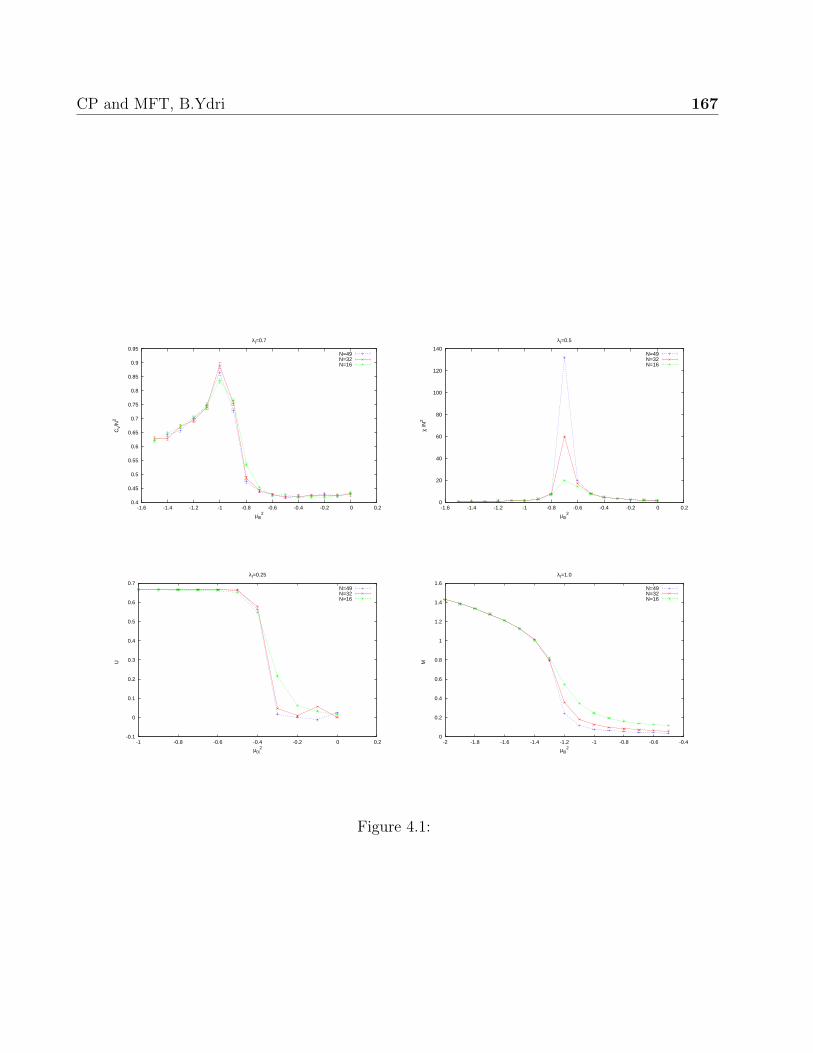
CP and MFT, B.Ydri 167
0.4
0.45
0.5
0.55
0.6
0.65
0.7
0.75
0.8
0.85
0.9
0.95
-1.6 -1.4 -1.2 -1 -0.8 -0.6 -0.4 -0.2 0 0.2
Cv/
N2
µ 0l2
λ l=0.7
N=49N=32N=16
0
20
40
60
80
100
120
140
-1.6 -1.4 -1.2 -1 -0.8 -0.6 -0.4 -0.2 0 0.2
χ /N
2
µ 0l2
λ l=0.5
N=49N=32N=16
-0.1
0
0.1
0.2
0.3
0.4
0.5
0.6
0.7
-1 -0.8 -0.6 -0.4 -0.2 0 0.2
U
µ 0l2
λ l=0.25
N=49N=32N=16
0
0.2
0.4
0.6
0.8
1
1.2
1.4
1.6
-2 -1.8 -1.6 -1.4 -1.2 -1 -0.8 -0.6 -0.4
M
µ 0l2
λ l=1.0
N=49N=32N=16
Figure 4.1:
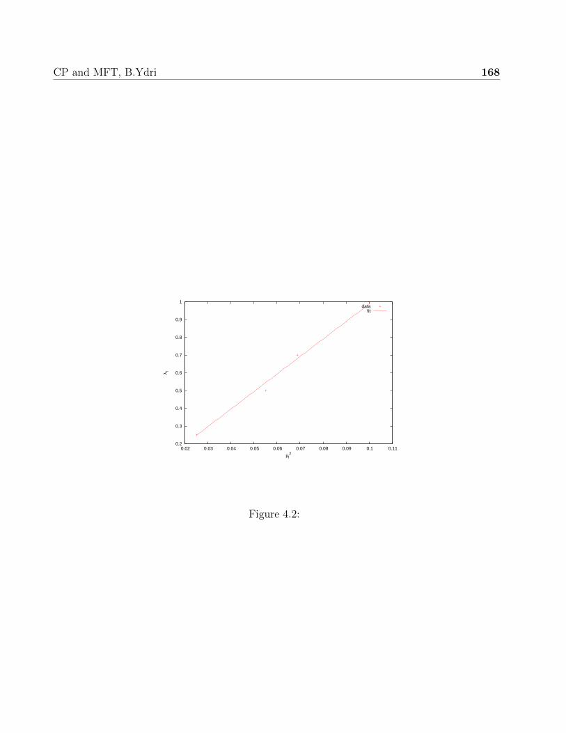
CP and MFT, B.Ydri 168
0.2
0.3
0.4
0.5
0.6
0.7
0.8
0.9
1
0.02 0.03 0.04 0.05 0.06 0.07 0.08 0.09 0.1 0.11
λ l
µ l2
datafit
Figure 4.2:
Bibliography
[1] J. Smit, “Introduction to quantum fields on a lattice: A robust mate,” Cambridge
Lect. Notes Phys. 15, 1 (2002).
[2] W. Loinaz and R. S. Willey, “Monte Carlo simulation calculation of critical coupling
constant for continuum phi**4 in two-dimensions,” Phys. Rev. D 58, 076003 (1998)
[hep-lat/9712008].
[3] D. Schaich and W. Loinaz, “An Improved lattice measurement of the critical coupling
in phi(2)**4 theory,” Phys. Rev. D 79, 056008 (2009) [arXiv:0902.0045 [hep-lat]].
[4] S. J. Chang, “The Existence of a Second Order Phase Transition in the Two-
Dimensional phi**4 Field Theory,” Phys. Rev. D 13, 2778 (1976) [Phys. Rev. D
16, 1979 (1977)].

Chapter 5
(Multi-Trace) Quartic Matrix
Models
5.1 The Pure Real Quartic Matrix Model
This is a very well known, and a very well studied, model which depends on a single
hermitian matrix M . This is given by
V = BTrM2 + CTrM4
=N
g(−TrM2 +
1
4TrM4). (5.1)
The model depends actually on a single coupling g such that
B = −Ng, C =
N
4g. (5.2)
There are two stable phases in this model:
Disordered phase (one-cut) for g ≥ gc: This is characterized by the eigenvalues
distribution of the matrix M given by
ρ(λ) =1
Nπ(2Cλ2 +B + Cδ2)
√δ2 − λ2
=1
gπ(1
2λ2 − 1 + r2)
√4r2 − λ2. (5.3)
This is a single cut solution with the cut defined by
− 2r ≤ λ ≤ 2r. (5.4)
r =1
2δ. (5.5)
δ2 =1
3C(−B +
√B2 + 12NC)
=1
3(1 +
√1 + 3g). (5.6)

CP and MFT, B.Ydri 171
Non-uniform ordered phase (two-cut) for g ≤ gc: This is characterized by the
eigenvalues distribution of the matrix M given by
ρ(λ) =2C|λ|Nπ
√(λ2 − δ2
1)(δ22 − λ2)
=|λ|2gπ
√(λ2 − r2
−)(r2+ − λ2). (5.7)
Here there are two cuts defined by
r− ≤ |λ| ≤ r+. (5.8)
r− = δ1 , r+ = δ2. (5.9)
r2∓ =
1
2C(−B ∓ 2
√NC)
= 2(1∓√g). (5.10)
A third order transition between the above two phases occurs at the critical point
gc = 1↔ B2c = 4NC ↔ Bc = −2
√NC. (5.11)
There is a third phase in this model: the so-called Ising or uniform ordered phase, which
despite the fact that it is not stable, plays an important role in generalizations of this
model, such as the one discussed in the next section, towards noncommutative Φ4.
5.2 The Multi-Trace Matrix Model
Our primary interest here is the theory of noncommutative Φ4 on the fuzzy sphere
given by the action
S =4πR2
N + 1Tr
(1
2R2Φ∆Φ +
1
2m2Φ2 +
λ
4!Φ4
). (5.12)
The Laplacian is ∆ = [La, [La, ...]]. Equivalently with the substitution Φ = M/√
2πθ,
where M =∑N
i,j=1Mij |i >< j|, this action reads
S = Tr
(aM∆M+ bM2 + cM4
). (5.13)
The parameters are1
a =1
2R2, b =
1
2m2 , c =
λ
4!
1
2πθ. (5.14)
1The noncommutativity parameter on the fuzzy sphere is related to the radius of the sphere by θ =
2R2/√N2 − 1.

CP and MFT, B.Ydri 172
In terms of the matrix M the action reads
S[M ] = r2K[M ] + Tr[bM2 + cM4
]. (5.15)
The kinetic matrix is given by
K[M ] = Tr
[− Γ+MΓM − 1
N + 1Γ3MΓ3M + EM2
]. (5.16)
The matrices Γ, Γ3 and E are given by
(Γ3)lm = lδlm , (Γ)lm =
√(m− 1)(1− m
N + 1)δlm−1 , (E)lm = (l − 1
2)δlm. (5.17)
The relationship between the parameters a and r2 is given by
r2 = 2aN (5.18)
We start from the path integral
Z =
∫dM exp
(− S[M ]
)
=
∫dΛ ∆2(Λ) exp
(− Tr
(bΛ2 + cΛ4
))∫dU exp
(− r2K[UΛU−1]
).(5.19)
The second line involves the diagonalization of the matrix M (more on this below). The
calculation of the integral over U ∈ U(N) is a very long calculation done in [2,3]. The end
result is a multi-trace effective potential given by (assuming the symmetry M −→ −M)
Seff =∑
i
(bλ2i + cλ4
i )−1
2
∑
i 6=jln(λi − λj)2
+
[r2
8v2,1
∑
i 6=j(λi − λj)2 +
r4
48v4,1
∑
i 6=j(λi − λj)4 − r4
24N2v2,2
[∑
i 6=j(λi − λj)2
]2+ ...
].
(5.20)
The coefficients v will be given below. If we do not assume the symmetry M −→ −Mthen obviously there will be extra terms with more interesting consequences for the phase
structure as we will discuss briefly below.
This problem (5.20) is a generalization of the quartic Hermitian matrix potential
model. Indeed, this effective potential corresponds to the matrix model given by
V =
(b+
aN2v2,1
2
)TrM2 +
(c+
a2N3v4,1
6
)TrM4 − 2ηa2N2
3
[TrM2
]2
. (5.21)
This can also be solved exactly as shown in [2]. The strength of the multi-trace term η is
given by
η = v2,2 −3
4v4,1. (5.22)

CP and MFT, B.Ydri 173
The coefficients v2,1, v4,1 and v2,2 are given by the following two competing calculations
of [2] and [3] given respectively by
v2,1 = 1 , v4,1 = 0 , v2,2 =1
8. (5.23)
v2,1 = −1 , v4,1 =3
2, v2,2 = 0. (5.24)
This discrepancy is discussed in [2].
5.3 Model and Algorithm
We thus start from the potential and the partition function
V = Tr
(BM2 + CM4
)+D
(TrM2
)2
. (5.25)
We may include the odd terms found in [2] without any real extra effort. We will not do
this here for simplicity, but we will include them for completeness in the attached code.
The partition function (path integral) is given by
Z =
∫dM exp
(− V
). (5.26)
The relationship between the two sets of parameters a, b, c and B,C,D is given by
B = b+aN2v2,1
2, C = c+
a2N3v4,1
6, D = −2ηa2N2
3. (5.27)
The collpased parameters are
B =B
N32
= b+av2,1
2, C =
C
N2= c+
a2v4,1
6, D = −2ηa2N
3. (5.28)
Only two of these three parameters are independent. For consistency of the large N
limit, we must choose a to be any fixed number. We then choose for simplicity a = 1 or
equivalently D = −2ηN/32.
We can now diagonalize the scalar matrix M as
M = UΛU−1. (5.29)
We compute
δM = U
(δΛ + [U−1δU,Λ]
)U−1. (5.30)
2The authors of [1] chose instead a = 1.

CP and MFT, B.Ydri 174
Thus (with U−1δU = iδV being an element of the Lie algebra of SU(N))
Tr(δM)2 = Tr(δΛ)2 + Tr[U−1δU,Λ]2
=∑
i
(δλi)2 +
∑
i 6=j(λi − λj)2δVijδV
∗ij . (5.31)
We count N2 real degrees of freedom as there should be. The measure is therefore given
by
dM =∏
i
dλi∏
i 6=jdVijdV
∗ij
√det(metric)
=∏
i
dλi∏
i 6=jdVijdV
∗ij
√∏
i 6=j(λi − λj)2. (5.32)
We write this as
dM = dΛdU∆2(Λ). (5.33)
The dU is the usual Haar measure over the group SU(N) which is normalized such that∫dU = 1, whereas the Jacobian ∆2(Λ) is precisely the so-called Vandermonde determinant
defined by
∆2(Λ) =∏
i>j
(λi − λj)2. (5.34)
The partition function becomes
Z =
∫dΛ ∆2(Λ) exp
(− Tr
(BΛ2 + CΛ4
)−D
(TrΛ2
)2). (5.35)
We are therefore dealing with an effective potential given by
Veff = B∑
i=1
λ2i + C
∑
i=1
λ4i +D
(∑
i=1
λ2i
)2
− 1
2
∑
i 6=jln(λi − λj)2. (5.36)
We will use the Metropolis algorithm to study this model. Under the change λi −→ λi+h
of the eigenvalue λi the above effective potential changes as Veff −→ Veff + ∆Vi,h where
∆Vi,h = B∆S2 + C∆S4 +D(2S2∆S2 + ∆S22) + ∆SVand. (5.37)
The monomials Sn are defined by Sn =∑
i λni while the variations ∆Sn and ∆SVand are
given by
∆S2 = h2 + 2hλi. (5.38)
∆S4 = 6h2λ2i + 4hλ3
i + 4h3λi + h4. (5.39)
∆SVand = −2∑
j 6=iln |1 +
h
λi − λj|. (5.40)

CP and MFT, B.Ydri 175
5.4 The Disorder-to-Non-Uniform-Order Transi-
tion
The pure quartic matrix model (5.1) is characterized by a third-order phase transition
between a disordered phase characterized by < M >= 0 and a non-uniform ordered
phase characterized by < M >= −Bγ/2C where γ is an N−dimensional idempotent, viz
γ2 = 1. This transition is also termed one-cut-to-two-cut transition. Thus the eigenvalues
distribution of the scalar field M will go from a one-cut solution centered around 0 in the
disordered phase to a two-cut solution with two peaks symmetric around 0 in the uniform
ordered phase. The transition should occur around g = gc = 1. This transition is critical
since the two different eigenvalues distributions in the two phases become identical at the
transition point.
Monte Carlo tests of the above effects, and other physics, can be done using the code
found in the last chapter. An illustration with 220 thermalized configurations, where
each two successive configurations are separated by 25 Monte Carlo steps to reduce auto-
correlation effects, and with N = 10 and g = 2, 1.5, 1, 0.5, is shown on figure (5.1). The
pure quartic matrix model is obtained from the multitrace matrix model by setting the
kinetic parameter a zero. We observe an excellent with the theoretical predictions (5.3)
and (5.7).
The above transition is third-order, as we said, since the first derivative of the specific
heat has a finite discontinuity at r = B/|Bc| = −1 as is obvious from the exact analytic
result
CvN2
=1
4, r < −1. (5.41)
CvN2
=1
4+
2r4
27− r
27(2r2 − 3)
√r2 + 3 , r > −1. (5.42)
This behavior is also confirmed in Monte Carlo simulation as shown for c = 4 and N = 8
and N = 10 on figure (5.2).
The above one-cut-to-two-cut transition persists largely unchanged in the quartic mul-
titrace matrix model (5.21). On the other hand, and similarly to the above pure quartic
matrix model, the Ising phase is not stable in this case and as a consequence the transition
between non-uniform order and uniform-order is not observed in Monte Carlo simulations.
The situation is drastically different if odd multitrace terms are included.

CP and MFT, B.Ydri 176
0
0.05
0.1
0.15
0.2
0.25
0.3
0.35
-6 -5 -4 -3 -2 -1 0 1 2 3 4 5
ρ (λ
)
λ
g=3,N=10theory
0
0.05
0.1
0.15
0.2
0.25
0.3
0.35
0.4
-6 -5 -4 -3 -2 -1 0 1 2 3 4 5
ρ (λ
)
λ
g=2,N=10theory
0
0.1
0.2
0.3
0.4
0.5
0.6
-6 -5 -4 -3 -2 -1 0 1 2 3 4 5
ρ (λ
)
λ
g=1,N=10theory
0
0.1
0.2
0.3
0.4
0.5
0.6
0.7
-6 -5 -4 -3 -2 -1 0 1 2 3 4 5
ρ (λ
)
λ
g=0.5,N=10theory
0
0.1
0.2
0.3
0.4
0.5
0.6
0.7
-3 -2 -1 0 1 2 3
ρ (λ
)
λ
g=3,N=10g=2,N=10g=1,N=10
g=0.5,N=10
Figure 5.1:
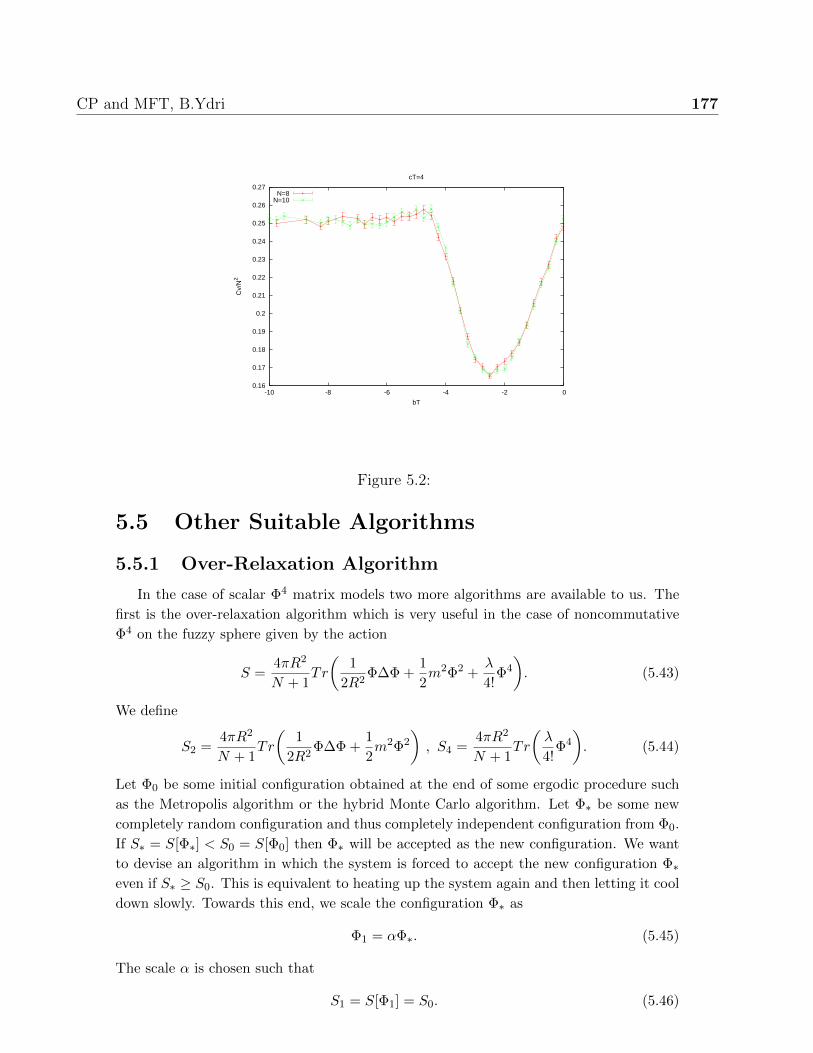
CP and MFT, B.Ydri 177
0.16
0.17
0.18
0.19
0.2
0.21
0.22
0.23
0.24
0.25
0.26
0.27
-10 -8 -6 -4 -2 0
Cv/
N2
bT
cT=4
N=8N=10
Figure 5.2:
5.5 Other Suitable Algorithms
5.5.1 Over-Relaxation Algorithm
In the case of scalar Φ4 matrix models two more algorithms are available to us. The
first is the over-relaxation algorithm which is very useful in the case of noncommutative
Φ4 on the fuzzy sphere given by the action
S =4πR2
N + 1Tr
(1
2R2Φ∆Φ +
1
2m2Φ2 +
λ
4!Φ4
). (5.43)
We define
S2 =4πR2
N + 1Tr
(1
2R2Φ∆Φ +
1
2m2Φ2
), S4 =
4πR2
N + 1Tr
(λ
4!Φ4
). (5.44)
Let Φ0 be some initial configuration obtained at the end of some ergodic procedure such
as the Metropolis algorithm or the hybrid Monte Carlo algorithm. Let Φ∗ be some new
completely random configuration and thus completely independent configuration from Φ0.
If S∗ = S[Φ∗] < S0 = S[Φ0] then Φ∗ will be accepted as the new configuration. We want
to devise an algorithm in which the system is forced to accept the new configuration Φ∗even if S∗ ≥ S0. This is equivalent to heating up the system again and then letting it cool
down slowly. Towards this end, we scale the configuration Φ∗ as
Φ1 = αΦ∗. (5.45)
The scale α is chosen such that
S1 = S[Φ1] = S0. (5.46)
CP and MFT, B.Ydri 178
Equivalently
S4∗α4 + S2∗α2 − S0 = 0. (5.47)
The solution is given by
if S0 > 0 : α2 =
√S2
2∗ + 4S0S4∗ − S2∗2S4∗
. (5.48)
if S0 < 0 and S2∗ < −√−4S0S4∗ < 0 : α2 =
±√S2
2∗ + 4S0S4∗ − S2∗2S4∗
. (5.49)
If the conditions in the above two equations are not met then we should redefine the
matrix Φ∗ iterativley as
Φ∗ −→Φ∗ + Φ0
2. (5.50)
Then repeat. This iterative procedure will obviously create unwanted autocorrelations
due to the fact that Φ∗ becomes closer in each iteration to Φ0. However, the process will
terminate in a finite number of steps and the obtained final configuration Φ1 has a greater
probability in falling in a different orbit than the original Φ0.
The claim of [5] is that this algorithm solves the ergodic problem observed in Monte
Carlo simulations of noncommutative Φ4 on the fuzzy sphere.
5.5.2 Heat-Bath Algorithm
The second algorithm is the heat-bath algorithm which works very nicely for the
unbounded Φ4 potential
V =N
g(TrM2 − 1
4TrM4). (5.51)
Remark the minus sign in front of the quartic term. Although this potential is unbounded
from below it has a well defined large N limit due to the metastability of the origin. The
path integral is given by
Z =
∫dM exp(−N
gTrM2) exp(
N
4gTrM4)
=
∫dMdQ exp(−N
gTrM2 − TrQ2 +
√N
gTrQM2). (5.52)
The matrices M and Q are fully Gaussian. Let us then consider a Gaussian distribution√a
π
∫dx exp(−ax2). (5.53)
The Gaussian random number x must be chosen, in any Monte Carlo routine, as
R =
√−1
aln(1− r1)
φ = 2πr2
x = R cosφ. (5.54)

CP and MFT, B.Ydri 179
The r1 and r2 are two uniform random numbers between 0 and 1.
The part of the above path integral which depends on Q is Gaussian given by
∫dQ exp(−Tr(Q− 1
2
√N
gM2)2). (5.55)
The diagonal element Qii comes with a factor a = 1 while the off diagonal elements comes
with a factor a = 2. Thus we choose
Qii = zii|a=1 +1
2
√N
g(M2)ii , Qij =
xij + iyij√2|a=1 +
1
2
√N
g(M2)ij . (5.56)
The x, y and z are Gaussian random numbers with a = 1.
The part of the path integral which depends on the diagonal element Mii is given by
∫ ∏
i
dMii exp∑
i
(− N
g(1−
√g
NQii)(Mii)
2 +1
2
√N
g
∑
j 6=i(QijMji +QjiMij)Mii
)=
∫ ∏
i
dMii exp∑
i
(− li(Mii −
hi2li
)2 + ...
).(5.57)
li =N
g(1−
√g
NQii) , hi =
1
2
√N
g
∑
j 6=i(QijMji +QjiMij). (5.58)
Thus the diagonal elements Mii are Gaussian numbers which come with factors a = li.
Thus we choose
Mii =xii√li|a=1 +
hi2li. (5.59)
Finally, the part of the path integral which depends on the off diagonal element Mij is
given by∫ ∏
i 6=jdMijdM
∗ij exp
∑
i 6=j
(− lijM∗ijMij + hijM
∗ij + h∗ijMij
)=
∫ ∏
i 6=jdMijdM
∗ij exp
∑
i 6=j
(− lij |Mij −
hijlij|2 + ...
). (5.60)
lij =N
g
(1− 1
2
√g
N(Qii +Qjj)
), hij =
1
4
√N
g
(∑
k 6=iQikMkj +
∑
k 6=jQkjMik
). (5.61)
Hence the off diagonal elementsMij are Gaussian numbers which come with factors a = lij .
Thus we choose
Mij =xij + iyij√
lij|a=1 +
hijlij. (5.62)
This algorithms can also be applied quite effectively to simple Yang-Mills matrix models
as done for example in [6, 7].

Bibliography
[1] F. Garcia Flores, X. Martin and D. O’Connor, “Simulation of a scalar field on a fuzzy
sphere,” Int. J. Mod. Phys. A 24, 3917 (2009) [arXiv:0903.1986 [hep-lat]].
[2] B. Ydri, “A Multitrace Approach to Noncommutative Φ42,” arXiv:1410.4881 [hep-th].
[3] D. O’Connor and C. Saemann, “Fuzzy Scalar Field Theory as a Multitrace Matrix
Model,” JHEP 0708, 066 (2007) [arXiv:0706.2493 [hep-th]].
[4] N. Kawahara, J. Nishimura and A. Yamaguchi, “Monte Carlo approach to nonpertur-
bative strings - Demonstration in noncritical string theory,” JHEP 0706, 076 (2007)
[hep-th/0703209].
[5] M. Panero, “Numerical simulations of a non-commutative theory: The Scalar model
on the fuzzy sphere,” JHEP 0705, 082 (2007) [hep-th/0608202].
[6] T. Hotta, J. Nishimura and A. Tsuchiya, “Dynamical aspects of large N reduced
models,” Nucl. Phys. B 545, 543 (1999) [hep-th/9811220].
[7] T. Azuma, S. Bal, K. Nagao and J. Nishimura, “Nonperturbative studies of fuzzy
spheres in a matrix model with the Chern-Simons term,” JHEP 0405, 005 (2004)
[hep-th/0401038].

Chapter 6
The Remez Algorithm and The
Conjugate Gradient Method
6.1 Minimax Approximations
The rational hybrid Monte Carlo algorithm (RHMC) uses in an essential way a rational
approximation to the fermionic determinant. Thus in this section we will first review the
issue of rational and polynomial approximations of functions. We will follow [4,5].
6.1.1 Minimax Polynomial Approximation and Chebyshev
Polynomials
Chebyshev norm: We start by introducing the Chebyshev norm (also called uniform,
infinity, supremum norm) of a continuous function f over the unit interval [0, 1] by the
relation
||f ||∞ = limn−→∞||f ||n
= limn−→∞
(∫ 1
0dx|f(x)|n
)1/n
= maxx|f(x)|. (6.1)
Minimax approximation: A minimax polynomial (or rational) approximation of f
is a polynomial (or rational) function p which minimizes the Chebyshev norm of p − f ,
viz
||p− f ||∞ = minpmaxx|p(x)− f(x)|. (6.2)
Weierstrass theorem: The fundamental theorem of approximation theorem is Weier-
strass theorem. This can be stated as follows. For every continuous function f(x) over
a closed interval [a, b], and for every specified tolerance ε > 0, there exists a polynomial
pn(x) of some degree n such that for all x ∈ [a, b], we have ||f(x)−pn(x)||∞ < ε. Thus any

CP and MFT, B.Ydri 182
continuous function can be arbitrarily well approximated by a polynomial. This means
in particular that the space of polynomials is dense in the space of continuous functions
with respect to the topology induced by the Chebyshev norm.
Chebyshev theorem (minimax polynomial approximation): We consider a
function f defined on the unit interval. For any given degree n, there exists always a
unique polynomial pn of degree n which minimizes the error function
||e||∞ = max0≤x≤1|e(x)| = max0≤x≤1|pn(x)− f(x)|, (6.3)
iff the error function e(x) takes its maximum absolute value at at least n + 2 points on
the unit interval, which may include the end points, and furthermore the sign of the error
alternate between the successive extrema.
We can go from the function f(x) defined in the interval [−1,+1] to a function f(y)
defined in a generic interval [a, b] by considering the transformation x −→ y given by
x =y − 1
2(b+ a)12(b− a)
. (6.4)
A simple proof of this theorem can be found in [4]. This goes as follows:
• Chebyshev’s criterion is necessary: If the error has fewer than n + 2
alternating extrema then the approximation can be improved. Let p(x) be
a polynomial for which the error e(x) = p(x)−f(x) has fewer than n+ 2 alternating
extrema. The next largest extremum of the error, corresponding to a local extremum,
is therefore smaller by some non zero gap ∆. Between any two successive alternating
extrema the error obviously will pass by zero at some point zi. If we assume that we
have d + 1 alternating extrema, then we will d zeros zi. We can trivially construct
the polynomial
u(x) = A∏
i
(x− zi). (6.5)
We choose A such that the sign of u(x) is opposite to the sign of e(x) and its
magnitude ∆′
is less than ∆, viz
u(xi)e(xi) < 0 , ∆′
= max0≤x≤1|u(x)| < ∆. (6.6)
We consider now the polynomial p′(x) = p(x) + u(x) with corresponding error func-
tion e′(x) = e(x) + u(x). The first condition u(xi)e(xi) < 0 yields directly to the
conclusion that the error e′(x) is less than e(x) in the domain of the alternating
extrema, whereas it is the condition ∆′< ∆ that yields to the conclusion that e
′(x)
is less than e(x) in the domain of the next largest extremum. Thus e′(x) < e(x)
throughout and hence p′(x) is a better polynomial approximation.
• Chebyshev’s criterion is sufficient: If the error is extremal at exactly
n+ 2 alternating points then the approximation is optimal. Let us assume
CP and MFT, B.Ydri 183
that there is another polynomial p′(x) which provides a better approximation. This
means that the uniform norm ||e′ ||∞ = max0≤x≤1|e′(x)| = max0≤x≤1|p′(x)− f(x)| isless than ||e||∞ = max0≤x≤1|e(x)| = max0≤x≤1|p(x) − f(x)|. Equivalently we must
have at the n+ 2 extrema of e(xi) the inequalities
|e′(xi)| < |e(xi)|. (6.7)
By the requirement of continuity there must therefore exist n+ 1 points zi between
the extrema at which we have
e′(zi) = e(zi). (6.8)
This leads immediately to
p′(zi) = p(zi). (6.9)
In other words, the polynomial p′(x)−p(x) has n+1 zeros, but since this polynomial
is of degree n, it must vanish identically. Hence p′(x) = p(x).
Chebyshev polynomials: The Chebyshev polynomial of degree n is defined by
Tn(cos θ) = cosnθ ↔ Tn(x) = cos(n cos−1 x). (6.10)
We have the explicit expressions
T0 = 1 , T1 = x , T2 = 2x2 − 1 , ... (6.11)
From the results Tn±1 = cosnθ cos θ ∓ sinnθ sin θ we deduce the recursion relation
Tn+1 = 2xTn − Tn−1. (6.12)
These polynomials are orthogonal in the interval [−1, 1] with a weight 1/(1− x2)1/2, viz
∫ +1
−1
dx√1− x2
Ti(x)Tj(x) =π
2δij . (6.13)
∫ +1
−1
dx√1− x2
T0(x)T0(x) = π. (6.14)
The zeros of the polynomial Tn(x) are given by
Tn(cos θ) = 0⇒ cosnθ = 0⇒ nθ = (2k − 1)π
2⇒ x = cos
(2k − 1)π
2n, k = 1, 2, ..., n.(6.15)
Since the angle θ is in the interval between 0 and π. There are therefore n zeros.
The derivative of Tn is given by
d
dxTn = −n d
dxcos−1 x. sin(n cos−1 x)
=n√
1− x2sin(n cos−1 x). (6.16)

CP and MFT, B.Ydri 184
The extrema of the polynomial Tn(x) are given by
d
dxTn = 0⇒ sin(nθ) = 0⇒ nθ = kπ ⇒ x = cos
kπ
n, k = 0, 2, ..., n. (6.17)
There are n+1 extrema. The maxima satisfy Tn(x) = 1 while the minima satisfy Tn(x) =
−1.
The Chebyshev polynomials satisfy also the following discrete orthogonality relation:
m∑
k=1
Ti(xk)Tj(xk) =m
2δij . (6.18)
m∑
k=1
T0(xk)T0(xk) = m. (6.19)
In the above two equations i, j < m and xk, k = 1, ...,m, are the m zeros of the Chebyshev
polynomial Tm(x).
Since Tn(x) has n+ 1 extrema which alternate in value between −1 and +1 for −1 ≤x ≤ 1, and since the leading coefficient of Tn(x) is 2n−1; the polynomial pn(x) = xn −21−nTn(x) is the best polynomial approximation of degree n − 1 with uniform weight
to the function xn over the interval [−1, 1]. This is because by construction the error
en(x) = pn(x) − xn = 21−nTn(x) satisfies Chebyshevs criterion. The magnitude of the
error is just ||en||∞ = 21−n = 2e−n ln 2, i.e. the error decreases exponentially with n.
Chebyshev approximation: Let f(x) be an arbitrary function in the interval [−1,+1].
The Chebyshev approximation of this function can be constructed as follows. Let N be
some large degree and xk, k = 1, ..., N , be the zeros of the Chebyshev polynomial TN (x).
The function f(x) can be approximated by the polynomial of order N defined by
fN (x) =N∑
k=1
ckTk−1(x)− 1
2c1. (6.20)
The coefficients ck are given by
cj =2
N
N∑
k=1
f(xk)Tj−1(xk). (6.21)
This approximation is exact for x equal to all of the N zeros of TN (x). Indeed, we can
show
N∑
k=1
Tl−1(xk)fN (xk) =N∑
k=1
ck
N∑
k=1
Tl−1(xk)Tk−1(xk)−1
2c1
N∑
k=1
Tl−1(xk)
=N
2cl , l = 1, ..., N. (6.22)
In other words,
fN (xk) = f(xk). (6.23)
CP and MFT, B.Ydri 185
For very large N , the polynomial fN becomes very close to the function f . The polynomial
fN can be ”gracefully”, by using the words of [5], truncated to a lower degree m << N
by considering
fm(x) =
m∑
k=1
ckTk−1(x)− 1
2c1. (6.24)
The error for rapidly decreasing ck, which is given by the difference between fN and fm, is
dominated by cm+1Tm which has m+1 equal extrema distributed smoothly and uniformly
in the interval [−1,+1]. Since the T ’s are bounded between −1 and +1 the total error
is the sum of the neglected ck, k = m+ 1, ..., N . The Chebyshev approximation fm(x) is
very close to the minimax polynomial which has the smallest maximum deviation from
the function f(x). Although the calculation of the Chebyshev polynomial fm(x) is very
easy, finding the actual minimax polynomial is very difficult in practice.
Economization of power series: This will be explained by means of a specific
example. We consider the function f(x) = sinx. A quintic polynomial approximation of
this function is given by the Taylor expansion
sinx = x− x3
6+
x5
120. (6.25)
The domain of definition of sinx can be taken to be the interval [−π, π]. By making
the replacement x −→ x/π we convert the domain of definition [−π, π] into the domain
[−1, 1], viz
sinx = πx− π3x3
6+π5x5
120. (6.26)
The error in the above quintic approximation is estimated by the first neglected term
evaluated at the end points x = ±1, viz
π7x7
7!|x=π = 0.6. (6.27)
The error in the 7th degree polynomial approximation can be found in the same way. We
get in this case π9x9/9!|x=π = 0.08.
The monomials xk can be given in terms of Chebyshev polynomials by the formulas
xk =1
2k−1
[Tk(x) +
k!
1!(k − 1)!Tk−2(x) +
k!
2!(k − 2)!Tk−4(x) + ...+
k!k−1
2 !(k − k−12 )!
T1(x)
], k odd.(6.28)
xk =1
2k−1
[Tk(x) +
k!
1!(k − 1)!Tk−2(x) +
k!
2!(k − 2)!Tk−4(x) + ...+
k!k2 !(k − k
2 )!T0(x)
], k even.(6.29)
For example
x = T1(x). (6.30)

CP and MFT, B.Ydri 186
x3 =1
4[T3(x) + 3T1(x)]. (6.31)
x5 =1
16[T5(x) + 5T3(x) + 10T1(x)]. (6.32)
By substitution we get the result
sinx = πx− π3x3
6+π5x5
120
=π(192− 24π2 + π3)
192T1 −
π3(16− π2)
384T3 +
π5
1920T5. (6.33)
Since |Tn| ≤ 1, the last term is of the order of 0.16. This is smaller than the error
found in the quintic approximation above. By truncating this term we obtain a cubic
approximation of the sine function given by
sinx =π(192− 24π2 + π3)
192T1 −
π3(16− π2)
384T3 (6.34)
By substituting the Chebyshev polynomials by their expressions in terms of the xk, and
then changing back to the interval [−π,+π], we obtain the cubic polynomial
sinx =383
384x− 5x3
32. (6.35)
By construction this cubic approximation is better than the above considered quintic
approximation.
6.1.2 Minimax Rational Approximation and Remez Algo-
rithm
Chebyshev theorem revisited: Chebyshev theorem can be extended to the case
of minimax rational approximation of functions as follows. Again we consider a function
f defined on the unit interval. For any given degree (n, d), there exists always a unique
rational function rn,d of degree (n, d) which minimizes the error function given by
||e||∞ = max0≤x≤1|e(x)| = max0≤x≤1|rn,d(x)− f(x)|, (6.36)
iff the error function e(x) takes its maximum absolute value at at least n + d + 2 points
on the unit interval, which may include the end points, and furthermore the sign of the
error alternate between the successive extrema.
A simple proof of this theorem can be found in [4]. As it can be shown rational
approximations are far more superior to polynomial ones since, for some functions and
some intervals, we can achieve substantially higher accuracy with the same number of
coefficients. However, it should also be appreciated that constructing the rational approx-
imation is much more difficult than the polynomial one.
CP and MFT, B.Ydri 187
We will further explain this very important theorem following the discussion of [5].
The rational function rn,d is the ratio of two polynomials pn and qd of degrees n and d
respectively, viz
rn,d(x) =pn(x)
qd(x). (6.37)
The polynomials pn and qd can be written as
pn(x) = α0 + α1x+ ...+ αnxn , qd(x) = 1 + β1x+ ...+ βdx
d. (6.38)
We will assume that rn,d is non degenerate, i.e. it has no common polynomial factors in
numerator and denominator. The error function e(x) is the deviation of rn,d from f(x)
with a maximum absolute value e, viz
e(x) = rn,d(x)− f(x) , e = max0≤x≤1|e(x)|. (6.39)
Equation (6.37) can be rewritten as
α0 + α1x+ ...+ αnxn = (f(x) + e(x))
(1 + β1x+ ...+ βdx
d
). (6.40)
There are n + d + 1 unknowns αi and βi plus one which is the error function e(x). We
can choose the rational approximation rn,x(x) to be exactly equal to the function f(x) at
n+ d+ 1 points xi in the interval [−1, 1],viz
f(xi) = rn,d(xi) , e(xi) = 0. (6.41)
As a consequence the n+ d+ 1 unknowns αi and βi will be given by the n+ d+ 1 linear
equations
α0 + α1xi + ...+ αnxni = f(xi)
(1 + β1xi + ...+ βdx
di
). (6.42)
This can be solved any standard method such as LU decomposition.
The points xi which are chosen in the interval [−1, 1] will generically be such that
there exists an extremum of the error function e(x) in each subinterval [xi, xi+1] plus two
more extrema at the endpoints ± − 1 for a total of n + d + 1 extrema. In general, the
magnitudes of r(x) at the extrema are not the same.
Alternatively, we can choose the rational approximation rn,x(x), at n + d + 1 points
xi, to be equal to f(x) + yi with some fixed values yi of the error function e(x). Equation
(6.42) becomes
α0 + α1xi + ...+ αnxni = (f(xi) + yi)
(1 + β1xi + ...+ βdx
di
). (6.43)
If we choose the xi to be the extrema of the error function e(x) then the yi will be exactly
±e where e is the maximal value of |e(x)|. We get then n+d+ 2 (not n+d+ 1) equations
for the unknowns αi, βi and e given by
α0 + α1xi + ...+ αnxni = (f(xi)± e)
(1 + β1xi + ...+ βdx
di
). (6.44)
The ± signs are due to the fact that successive extrema are alternating between −e and
+e. Although, this is not exactly a linear system since e enters non linearly, it can still
be solved using for example methods such as Newton-Raphson.
CP and MFT, B.Ydri 188
Remez algorithm: A practical constructive approach to the minimax rational ap-
proximation of functions is given by Remez (or Remes) algorithm. This is a very difficult
algorithm to get to work completely and properly and some people such as the authors [5]
dislike it.
The Remez algorithm involves two nested iterations; the first on e and the second on
the xi’s. Explicitly, it goes through the following steps:
• We choose or guess n+ d+ 2 initial values of the points xi in the interval [0, 1]. The
goal is to make these points converge to the alternating extrema discussed above.
• The first iteration: We keep the xi’s fixed and find the best rational approximation
which goes through the points (xi, f(xi) + (−1)i∆). Towards this end, we need to
solve the n+ d+ 2 equations
α0 + α1xi + ...+ αnxni = (f(xi) + (−1)i∆))
(1 + β1xi + ...+ βdx
di
). (6.45)
The unknowns are αi, βi and ∆. We write this equation as
Mv = 0. (6.46)
The (n+ d+ 2)−dimensional vector v is formed from the coefficients αi, i = 0, ..., n
and βj , j = 0, ..., d with β0 = 1. This linear system has a non trivial solution iff
detM = 0. This condition is a polynomial in ∆. The real roots of this polynomial
are the allowed values of ∆ and each one of them will correspond to a solution αi and
βj . Each solution (αi, βj) corresponds to a certain rational approximation rn,d(x).
We pick the solution which minimizes the error function.
• The second iteration: We keep e or ∆ fixed and choose a new set of points xi’s
which is the best alternating set for e(x). This is done as follows. We choose an
arbitrary partition Ii of the interval [0, 1] where Ii is such that xi ∈ Ii. Then we
choose a new set of points x′i such that
x′i ∈ Ii , (−1)ie(x
′i) = maxx∈Ii(−1)ie(xi). (6.47)
Several drawbacks of this algorithm are noted in [4,5]. Among these, we mention here the
slow rate of convergence and the necessity of multiple precision arithmetic.
Zolotarevs Theorem: The case of rational approximations of the sign function, the
square root and the inverse square root are known analytically in the sense that the coef-
ficients of the optimal and unique Chebyshev rational approximations are known exactly.
This result is due to Zolotarev.
The Numerical Recipes algorithm: A much simpler but very sloppy approxi-
mation, which is claimed in [5] to be ”within a fraction of a least significant bit of the
minimax one”, and in which we try to bring the error not to zero as in the minimax case
but to ± some consistent value, can be constructed as follows:
CP and MFT, B.Ydri 189
• We start from n+d+ 1 values of xi, or even a larger number of xi, which are spaced
approximately like the zeros of a higher order Chebyshev polynomials.
• We solve for αi and βj the linear system:
α0 + α1xi + ...+ αnxni = f(xi)
(1 + β1xi + ...+ βdx
di
). (6.48)
In the case that the number of xi’s is larger than n+ d+ 1 we can use the singular
value decomposition method to solve this system. The solution will provide our
starting rational approximation rn,d(x). Compute e(xi) and e.
• We solve for αi and βj the linear system:
α0 + α1xi + ...+ αnxni = (f(xi)± e)
(1 + β1xi + ...+ βdx
di
). (6.49)
The ± is chosen to be the sign of the observed error function e(xi) at each point xi.
• We repeat the second step several times.
6.1.3 The Code ”AlgRemez”
This code can be found in [6].
6.2 Conjugate Gradient Method
6.2.1 Construction
Our presentation of the conjugate gradient method in this section will follow the ped-
agogical note [1]. See also [2, 3].
The basic problem: We consider a symmetric and positive definite n × n matrix A
and an n−dimensional vector ~v. The basic problem here is to solve for the n−dimensional
vector ~x which satisfies the equation
A~x = ~v. (6.50)
We will find the solution by means of the conjugate gradient method which is an iterative
algorithm suited for large sparse matrices A.
Principles of the method: The above problem is equivalent to finding the minimum
~x of the function Φ(~x) defined by
Φ(~x) =1
2~xA~x− ~x~v. (6.51)
The gradient of Φ is given by
~∇Φ(~x) = A~x− ~v. (6.52)
CP and MFT, B.Ydri 190
This vanishes at the minimum. If not zero, it gives precisely the direction of steepest
ascent of the surface Φ. The residual of the above set of equations is defined by
~r = −~∇Φ(~x) = ~v −A~x. (6.53)
We will denote the n linearly independent vectors in the vector space to which ~x belongs
by ~p(i), i = 1, ..., n. They form a basis in this vector space. The vector ~x can be expanded
as
~x =n∑
i=1
si~p(i) = P~s. (6.54)
P is the n× n matrix of the linearly independent vectors ~p(i), i.e. Pij = p(j)i , and ~s is the
vector of the coefficients si. Typically, we will start from a reference vector ~x0. Thus we
write
~x = ~x0 + P~s. (6.55)
The vectors ~p(i) are A−conjugate to each other iff
~p(i)A~p(j) = 0 , i 6= j. (6.56)
Thus we can write
P TAP = D. (6.57)
D is a diagonal matrix with elements given by
di = ~p(i)A~p(i). (6.58)
The gradient of Φ takes the form
~∇Φ = AP~s− ~r0 , ~r0 = ~v −A~x0. (6.59)
Next, multiplication with the transpose P T yields
P T ~∇Φ = P TAP~s− P T~r0
= D~s− P T~r0. (6.60)
The solution to ~∇Φ = 0 is then
D~s− P T~r0 = 0⇒ si =~p(i)~r0
~p(i)A~p(i). (6.61)
The solution si found by globally minimizing Φ, also locally minimizes Φ along the direc-
tion ~p(i). Thus starting from a vector ~x0 we obtain the solution
~x1 = ~x0 + s1~p(1) , s1 =
~p(1)~r0
~p(1)A~p(1), ~r0 = ~v −A~x0. (6.62)

CP and MFT, B.Ydri 191
This is the local minimum of Φ along a line from ~x0 in the direction ~p(1). Indeed, we can
check that
~p(1)~∇Φ = 0⇒ s1 =~p(1)~r0
~p(1)A~p(1). (6.63)
The vector ~r0 is the first residual at the point ~x0 given by
~∇Φ|~x0= −~r0. (6.64)
Next, starting from the vector ~x1 we obtain the solution
~x2 = ~x1 + s2~p(2) , s2 =
~p(2)~r1
~p(2)A~p(2), ~r1 = ~v −A~x1. (6.65)
This is the local minimum of Φ along a line from ~x1 in the direction ~p(2). The vector ~r1
is the new residual at the point ~x1, viz
~∇Φ|~x1= −~r1. (6.66)
In general starting from the vector ~xi we obtain the solution
~xi+1 = ~xi + si+1~p(i+1) , si+1 =
~p(i+1)~ri
~p(i+1)A~p(i+1), ~ri = ~v −A~xi. (6.67)
This is the local minimum of Φ along a line from ~xi in the direction ~p(i+1). The vector ~riis the residual at the point ~xi, viz
~∇Φ|~xi = −~ri. (6.68)
The residual vectors provide the directions of steepest descent of the function Φ at each
iteration step. Thus if we know the conjugate vectors ~p(i) we can compute the coefficients
si and write down the solution ~x. Typically, a good approximation of the true minimum
of Φ may be obtained only after a small subset of the conjugate vectors are visited.
Choosing the conjugate vectors: The next step is to choose a set of conjugate
vectors. An obvious candidate is the set of eigenvectors of the symmetric matrix A.
However, in practice this choice is made as follows. Given that we have reached the
iteration step i, i.e. we have reached the vector ~xi which minimizes Φ in the direction ~p(i),
the search direction ~p(i+1) will be naturally chosen in the direction of steepest descent of
the function Φ at the point ~xi, which since A is positive definite is given by the direction
of the residual ~ri, but conjugate to the previous search direction ~p(i). We start then from
the ansatz
~p(i+1) = ~ri − λ~p(i). (6.69)
This must be A−conjugate to ~p(i), viz
~p(i)A~p(i+1) = 0. (6.70)

CP and MFT, B.Ydri 192
This yields the value
λ =~p(i)A~ri
~p(i)A~p(i). (6.71)
The gradient ~∇Φ at the point ~xi is orthogonal to all previous search directions ~p(j), j < i.
Indeed, we compute
~p(j)~∇Φ|~xi = ~p(j)(A~xi − ~v
)
= ~p(j)(A~x0 +
i∑
k=1
skA~p(k) − ~v
)
= ~p(j)( i∑
k=1
skA~p(k) − ~r0
)
=i∑
k=1
sk~p(j)A~p(k) − ~p(j)~r0
= sj~p(j)A~p(j) − ~p(j)~r0
= 0. (6.72)
This formula works also for j = i. The gradients ~∇Φ|~xi is also orthogonal to all previous
gradients ~∇Φ|~xj , j < i. Indeed, we have
~∇Φ|~xj ~∇Φ|~xi = −~rj ~∇Φ|~xi= −(λ~p(j) + ~p(j+1))~∇Φ|~xi= 0. (6.73)
The first search direction can be chosen arbitrarily. We can for example choose ~p(1) =
~r0 = −~∇Φ|~x0. The next search direction ~p(2) is by construction A−conjugate to ~p(1).
At the third iteration step we obtain ~p(3) which is A−conjugate to ~p(2). The remaining
question is whether ~p(3) is A−conjugate to ~p(1) or not. In general we would like to show
that the search direction ~p(i) generated at the ith iteration step, which is A−conjugate to
~p(i−1), is also A−conjugate to all previously generated search directions ~p(j), j < i − 1.
Thus we need to show that
~p(j)A~p(i) = 0 , j < i− 1. (6.74)
We compute
~p(j)A~p(i) = ~p(j)A(~ri−1 − λ~p(i−1))
= ~p(j)A~ri−1 − λ~p(j)A~p(i−1)
=1
sj(~xj − ~xj−1)A~ri−1 − λ~p(j)A~p(i−1)
=1
sj(−~rj + ~rj−1)~ri−1 − λ~p(j)A~p(i−1)
= −λ~p(j)A~p(i−1)
= 0. (6.75)

CP and MFT, B.Ydri 193
Summary: Let us now summarize the main ingredients of the above algorithm. We
have the following steps:
1) We choose a reference vector ~x0. We calculate the initial residual ~r0 = ~v −A~x0.
2) We choose the first search direction as ~p(1) = ~r0.
3) The first iteration towards the solution is
~x1 = ~x0 + s1~p(1) , s1 =
~p(1)~r0
~p(1)A~p(1). (6.76)
4) The above three steps are iterated as follows:
~ri = ~v −A~xi. (6.77)
~p(i+1) = ~ri − λ~p(i) , λ =~p(i)A~ri
~p(i)A~p(i). (6.78)
si+1 =~p(i+1)~ri
~p(i+1)A~p(i+1). (6.79)
~xi+1 = ~xi + si+1~p(i+1). (6.80)
By using equations (6.77) and (6.80) we can show that equation (6.77) can be re-
placed by the equation
~ri = ~ri−1 − siA~p(i) (6.81)
Also we can derive the more efficient formulas
si+1 =~ri~ri
~p(i+1)A~p(i+1), λ = − ~ri~ri
~ri−1~ri−1. (6.82)
5) The above procedure continues as long as |~r| ≥ ε where ε is some tolerance, otherwise
stop.
6.2.2 The Conjugate Gradient Method as a Krylov Space
Solver
We start this section by introducing some slight change of notation. By making the
replacements ~p(i+1) −→ ~pi, si+1 −→ −βi, λ −→ −αi the conjugate gradient algorithm will
read
~xi+1 = ~xi − βi~pi , βi = − ~ri~ri~piA~pi
. (6.83)
~ri+1 = ~ri + βiA~pi. (6.84)

CP and MFT, B.Ydri 194
~pi+1 = ~ri+1 + αi+1~pi , αi+1 =~ri+1~ri+1
~ri~ri. (6.85)
We start iterating from
~x0 = 0 , ~r0 = ~v −A~x0 = ~v , ~p0 = ~r0 = ~v. (6.86)
Remark now the following. We have
~r0 = ~v −A~x0 ∈ span~r0. (6.87)
~r1 = ~r0 + β0A~r0 ∈ span~r0, A~r0. (6.88)
~r2 = ~r0 + β0A~r0 + β1A(~r0 + β0A~r0) + α1β1A~r0 ∈ span~r0, A~r0, A2~r0. (6.89)
In general we will have
~rn = Pn(A)~r0 ∈ span~r0, A~r0, A2~r0, ..., A
n~r0. (6.90)
The Pn(A) is a polynomial of degree n which obviously satisfy Pn(0) = 1. It is called
the residual polynomial. On the other hand, the space span~r0, A~r0, ..., An~r0 is called
a Krylov subspace. Since the residues ~rn are orthogonal the polynomials Pn(A) are also
orthogonal.
Similarly, we observe that
~p0 = ~r0 ∈ span~r0. (6.91)
~p1 = ~r1 + α1~r0 ∈ span~r0, A~r0. (6.92)
~p2 = ~r2 + α2~r1 + α1α2~r0 ∈ span~r0, A~r0, A2~r0. (6.93)
Thus in general
~pn ∈ span~r0, A~r0, A2~r0, ..., A
n~r0. (6.94)
Also
~xn = ~x0 −n−1∑
i=0
βi~pi. (6.95)
Thus
~xn − ~x0 = Qn−1(A)~r0 ∈ span~r0, A~r0, A2~r0, ..., A
n−1~r0. (6.96)
The Qn−1(A) is a polynomial of exact degree n − 1. Hence both the conjugate gradient
directions ~pn and the solutions ~xn − ~x0 belong to various Krylov subspaces.
The conjugate gradient method is an example belonging to a large class of Krylov
subspace methods. It is due to Hestenes and Stiefel [8] and it is the method of choice for
solving linear systems that are symmetric positive definite or Hermitian positive definite.
We conclude this section by the following two definitions.

CP and MFT, B.Ydri 195
Definition 1: Given a non-singular matrix A ∈ Cn×n and a non-zero vector r ∈ Cn,
the nth Krylov (sub)space Kn(A, r) generated by A from r is
Kn(A, r) = span(r,Ar, ..., An−1r). (6.97)
Definition 2: A standard Krylov space method for solving a linear system Ax = b is
an iterative method which starts from some initial guess x0 with residual r0 = b − Ax0
and then generates better approximations xn to the exact solution x∗ as follows
xn − x0 = Qn−1(A)r0 ∈ Kn(A, r0) = spanr0, Ar0, A2r0, ..., A
n−1r0. (6.98)
The residuals rn of the above so-called Krylov space solver will satisfy
rn = Pn(A)r0 ∈ Kn+1(A, r0) = spanr0, Ar0, A2r0, ..., A
nr0. (6.99)
It is not difficult to show that
Pn(A) = 1−AQn−1(A). (6.100)
6.2.3 The Multi-Mass Conjugate Gradient Method
The goal now is to solve a multi-mass linear system of the form
(A+ σ)~x = ~v. (6.101)
By a direct application of the conjugate gradient method we get the solution
~xσi+1 = ~xσi − βσi ~pσi , βσi = − ~rσi ~rσi
~pσi (A+ σ)~pσi. (6.102)
~rσi+1 = ~rσi + βσi (A+ σ)~pσi . (6.103)
~pσi+1 = ~rσi+1 + ασi+1~pσi , α
σi+1 =
~rσi+1~rσi+1
~rσi ~rσi
. (6.104)
~xσ0 = 0 , ~rσ0 = ~vσ − (A+ σ)~xσ0 = ~v , ~pσ0 = ~rσ0 = ~v. (6.105)
There is clearly a loop over σ which could be very expensive in practice. Fortunately we
can solve, by following [7], the above multi-mass linear system using only a single set of
vector-matrix operations as follows. First we note that
~rσi+1 = ~rσi + βσi (A+ σ)~pσi = P σi+1(A+ σ)~rσ0 ∈ Ki+2(A+ σ,~r0). (6.106)
As discussed before the polynomials P σi+1 are orthogonal in A+ σ. This follows from the
fact that ~rσi+1 ⊥ ~rσi and as a consequence
P σi+1(A+ σ)~rσ0 ⊥ Ki+1(A+ σ,~r0). (6.107)

CP and MFT, B.Ydri 196
However, we have the obvious and fundamental fact that
Ki+1(A+ σ,~r0) = Ki+1(A,~r0). (6.108)
In other words, the polynomials P σi+1 are orthogonal in A as well. We must therefore have
P σi+1(A+ σ) = ζσi+1Pi+1(A). (6.109)
The polynomials P σi+1 are thus of a shifted structure. By the identity (6.100) it follows
that the polynomials Qσi are not of a shifted structure. This single observation will allow
us to reduce the problem to a single set of vector-matrix operations.
By multiplying equation (6.104) by βσi+1(A+ σ) and using equation (6.103) we get
βσi+1(A+ σ)~pσi+1 = βσi+1(A+ σ)~rσi+1 +βσi+1α
σi+1
βσi(~rσi+1 − ~rσi ). (6.110)
By substitution in equation (6.103) we get the 3−term recurrence given by
~rσi+2 = (1 +βσi+1α
σi+1
βσi)~rσi+1 + βσi+1(A+ σ)~rσi+1 −
βσi+1ασi+1
βσi~rσi . (6.111)
By using (6.109) we obtain
ζσi+2~ri+2 = (1 +βσi+1α
σi+1
βσi)ζσi+1~ri+1 + βσi+1(A+ σ)ζσi+1~ri+1 −
βσi+1ασi+1
βσiζσi ~ri. (6.112)
However, the no-sigma recurrence reads
~ri+2 = (1 +βi+1αi+1
βi)~ri+1 + βi+1A~ri+1 −
βi+1αi+1
βi~ri. (6.113)
By comparing the A~ri+1 terms we obtain
βσn = βnζσn+1
ζσn. (6.114)
By comparing the ~ri terms and also using the above result we obtain
ασn = αnζσnβ
σn−1
ζσn−1βn−1. (6.115)
By comparing the ~ri+1 terms and also using the above two results we find after some
calculation
ζσn+1 =ζσnζ
σn−1βn−1
αnβn(ζσn−1 − ζσn ) + ζσn−1βn−1(1− σβn). (6.116)
Let us conclude by summarizing the main ingredients of this algorithm. These are:
1. We start from
~x = ~xσ0 = 0 , ~r0 = ~rσ0 = ~v , ~p = ~pσ0 = ~v. (6.117)
By setting i = −1 in (6.112) we see that we must also start from
α0 = ασ0 = 0 , β−1 = βσ−1 = 1 , ζσ0 = ζσ−1 = 1. (6.118)

CP and MFT, B.Ydri 197
2. We solve the no-sigma problem (we start from n = 0):
βn = − ~rn~rn~pnA~pn
~xn+1 = ~xn − βn~pn. (6.119)
~rn+1 = ~rn + βnA~pn. (6.120)
αn+1 =~rn+1~rn+1
~rn~rn~pn+1 = ~rn+1 + αn+1~pn. (6.121)
3. We generate solutions of the sigma problems by the relations (we start from n = 0):
ζσn+1 =ζσnζ
σn−1βn−1
αnβn(ζσn−1 − ζσn ) + ζσn−1βn−1(1− σβn). (6.122)
βσn = βnζσn+1
ζσn. (6.123)
~xσn+1 = ~xσn − βσn~pσn. (6.124)
~rσn+1 = ζσn+1~rn+1. (6.125)
ασn+1 = αn+1ζσn+1β
σn
ζσnβn. (6.126)
~pσn+1 = ~rσn+1 + ασn+1~pσn. (6.127)
Remark how the residues are generated directly from the residues of the no-sigma
problem.
4. The above procedure continues as long as |~r| ≥ ε where ε is some tolerance, otherwise
stop. Thus
|~r| ≥ ε , continue. (6.128)
We finally note that in the case of a hermitian matrix, i.e. A+ = A, we must replace
in the above formulas the transpose by hermitian conjugation. For example, we replace
~pTnA~pn by ~p+nA~p. The rest remains unchanged.

Bibliography
[1] E. Thompson, “The Conjugate Gradient Method: A Tutorial Note”.
[2] Martin H. Gutknecht, “A Brief Introduction to Krylov Space Methods for Solving
Linear Systems”.
[3] L. Chen, “Iterative Methods Based on Krylov Space”.
[4] A. D. Kennedy, “Approximation theory for matrices,” Nucl. Phys. Proc. Suppl.
128C, 107 (2004) [hep-lat/0402037].
[5] W. H. Press, S. A. Teukolsky, W. T. Vetterling and B. P. Flannery, “Numerical
Recipes in FORTRAN: The Art of Scientific Computing,” ISBN-9780521430647.
[6] M. A. Clark and A. D. Kennedy, https://github.com/mikeaclark/AlgRemez, 2005.
[7] B. Jegerlehner, “Krylov space solvers for shifted linear systems,” hep-lat/9612014.
[8] M. R. Hestenes and E. Stiefel, “Methods of conjugate gradients for solving linear
systems,” J. Res. Nat. Bureau Standards, 49:409435, 1952.

Chapter 7
Monte Carlo Simulation of
Fermion Determinants
As it is well known, simulation of fermion determinants and Pfaffians is crucial to
lattice QCD, but as it trurns out, it is also crucial to all supersymmetric matrix models
and quantum mechanical matrix models encountered or needed in matrix field theory,
matrix/fuzzy geometry and matrix formulation of noncommutative geometry, supersym-
metry and strings. As done before in this part of the book, the theoretical background
will be kept to a minimum, otherwise we will stray too far afield, and we will mostly focus
on practical problems. The main reference for this chapter is [1, 2]. See also [3, 4]. For
some subtle details of the rational hybrid Monte Carlo algorithm see [5–8].
7.1 The Dirac Operator
The basic problem we want to solve in this section is to simulate the partition function
of N = 1 supersymmetric Yang-Mills matrix model in d = 4 dimensions given by
ZYM =
∫ 4∏
µ=1
Xµ dθdθ exp
(θ(i[X4, ..] + σa[Xa, ..] + ξ
)θ
)exp(−SBYM[X]). (7.1)
SBYM = −Nγ4
4∑
µ,ν=1
Tr[Xµ, Xν ]2. (7.2)
The parameter γ will be set to one and we may add to the bosonic Yang-Mills action a
Chern-Simons term and a harmonic oscillator term with parameters α and m2 respectively.
The spinors θ and θ are two independent complex two-component Weyl spinors. They
contain the same number of degrees of Freedom as the four-component real Majorana
spinors in four dimensions. The scalar curvature or fermion mass parameter is given by ξ.
The above theory is only supersymmetric for a restricted set of values of the parameters
γ, α, m2 and ξ. See [11] and references therein for a discussion of this matter.
CP and MFT, B.Ydri 200
We have considered above the Dirac operator given by
D = iX4 − iXR4 + σaXa − σaXR
a + ξ. (7.3)
The determinant of this Dirac operator is positive definite since the eigenvalues come in
complex conjugate pairs [1]. In d = 6 and d = 10 the determinant is, however, complex
valued which presents a serious obstacle to numerical evaluation. In these three cases,
i.e. for d = 4, 6, 10, the supersymmetric path integral is well behaved. In d = 3 the
supersymmetric path integral is ill defined and only the bosonic ”quenched” approximation
makes sense. The source of the divergence lies in the so-called flat directions, i.e. the set
of commuting matrices. See [10] and references therein.
It is possible to rewrite the Dirac action in the following form (with X34 = X3 + iX4
and X± = X1 ± iX2)
TrθDθ = Tr
[θ1(X34 + ξ)θ1 + θ1X−θ2 + θ2X+θ1 + θ2(−X+
34 + ξ)θ2
]
− Tr
[X34θ1θ1 +X−θ1θ2 +X+θ2θ1 −X+
34θ2θ2
]. (7.4)
We expand the N ×N matrices θ1, θ2 and θ1, θ2 as
θα =N2∑
A=1
θAαTA , θα =
N2∑
A=1
θAαTA. (7.5)
The N ×N matrices TA are defined by
(TA)ij = δiiAδjjA , A = N(iA − 1) + jA. (7.6)
Then we find that
TrθDθ = χ1M11χ1 + χ1M12χ2 + χ2M21χ2 + χ2M22χ2. (7.7)
The N2−dimensional vectors χ1, χ2 and χ1, χ2 are defined by (χα)A = θAα and (χα)A =
θAα . The matrices MABαβ are N2 ×N2 defined by
(M11)AB = TrTA(X34 + ξ)TB − TrX34TATB. (7.8)
(M12)AB = TrTAX−TB − TrX−TATB. (7.9)
(M21)AB = TrTAX+TB − TrX+T
ATB. (7.10)
(M22)AB = TrTA(−X+34 + ξ)TB + TrX+
34TATB. (7.11)
We remark that
TrTAXTB − TrXTATB = XjAiBδiAjB −XjBiAδjAiB . (7.12)

CP and MFT, B.Ydri 201
Tr(TA)+TB = δiAiBδjAjB = δAB , T rTATB = δjAiBδjBiA = δAB. (7.13)
In the above two equations A and B are such that
A = N(jA − 1) + iA , B = N(iB − 1) + jB. (7.14)
In summary, the Dirac operator in terms of the 2N2−dimensional vectors χ and χ becomes
TrθDθ = χMχ. (7.15)
Next, we observe that the trace parts of the matrices Xa drop from the partition function.
Thus the measure should read∫dXaδ(TrXa) instead of simply
∫dXa. Similarly, we
observe that if we write θ = θ0 + η1, then the trace part η will decouple from the rest
since
Trθ
(i[X4, ..] + σa[Xa, ..] + ξ
)θ = Trθ0
(i[X4, ..] + σa[Xa, ..] + ξ
)θ0 + ξηη. (7.16)
Hence, the constant fermion modes ηα can also be integrated out from the partition func-
tion and thus we should consider the measure∫dθdθδ(Trθα)δ(Trθα) instead of
∫dθdθ.
These facts should be taken into account in the numerical study. We are thus led to
consider the partition function
ZYM =
∫ 4∏
µ=1
dXµ δ(TrXµ) detD exp(− SBYM[X]
). (7.17)
The determinant is given by
detD =
∫dθdθδ(Trθα)δ(Trθα) exp
(TrθDθ
)
=
∫dχdχδ
( N2∑
A=1
(χα)AδiAjA
)δ
( N2∑
A=1
(χα)AδiAjA
)exp
(χMχ
)
=
∫dχ′dχ′exp
(χ′M′
χ′). (7.18)
The vectors χ′α, χ
′α are (N2 − 1)−dimensional. The matrix M′
is 2(N2 − 1)× 2(N2 − 1)
dimensional, and it is given by
M′A′B′
αβ =MA′B′
αβ −MN2B′
αβ δiA′ jA′ −MA
′N2
αβ δiB′ jB′ +MN2N2
αβ δiA′ jA′ δi
B′ jB′ . (7.19)
We remark that
MN2N2
αβ = ξδαβ. (7.20)
Thus we must have
detD = detM′. (7.21)
CP and MFT, B.Ydri 202
The partition function thus reads
ZYM =
∫ 4∏
µ=1
dXµ δ(TrXµ) exp(− SYM[X]
). (7.22)
SYM[X] = SBYM[X] + V [X] , V = − ln detM′. (7.23)
We will need
∂SBYM
∂(Xµ)ij(t)= −Nγ
4∑
ν=1
[Xν , [Xµ, Xν ]]ji
= −Nγ(
2XνXµXν −X2νXµ −XµX
2ν
)
ji
. (7.24)
The determinant is real positive definite since the eigenvalues are paired up. Thus, we
can introduce the positive definite operator ∆ by
∆ = (M′)+M′
. (7.25)
The action V can be rewritten as
V = −1
2ln det ∆. (7.26)
The leap-frog algorithm for this problem is given by
(Pµ)ij(n+1
2) = (Pµ)ij(n)− δt
2
[∂SBYM
∂(Xµ)ij(n) + (Vµ)ij(n)
]. (7.27)
(Xµ)ij(n+ 1) = (Xµ)ij(n) + δt(Pµ)ji(n+1
2). (7.28)
(Pµ)ij(n+ 1) = (Pµ)ij(n+1
2)− δt
2
[∂SBYM
∂(Xµ)ij(n+ 1) + (Vµ)ij(n+ 1)
]. (7.29)
The effect of the determinant is encoded in the matrix
(Vµ)ij =∂V
∂(Xµ)ij
= −1
2Trad∆−1 ∂∆
∂(Xµ)ij. (7.30)
From (7.23) and (7.30) we see that we must compute the inverse and the determinant of
the Dirac operator at each hybrid Monte Carlo step. However, the Dirac operator is an
N × N matrix where N = 2N2 − 2. This is proportional to the number of degrees of
freedom. Since the computation of the determinant requires O(N 3) operations at best,
through Gaussian elimination, we see that the computational effort of the above algorithm
will be O(N6). Recall that the computational effort of the bosonic theory is O(N3)1 .
1Compare also with field theory in which the number of degrees of freedom is proportional to the volume, the
computational effort of the bosonic theory is O(V ) while that of the full theory, which includes a determinant,
is O(V 2).
CP and MFT, B.Ydri 203
7.2 Pseudo-Fermions and Rational Approximations
We introduce pseudo-fermions in the usual way as follows. The determinant can be
rewritten in the form
detD = detM′= (det ∆)
12
=
∫dφ+dφ exp(−φ+∆−1/2φ). (7.31)
Since D, M′ and ∆ are N × N matrices organized as 2 × 2 matrices, with components
given by N × N matrices where N = N/2, the vectors φ+ and φ can be thought of as
two-component spinors where each component is given by an N−dimensional vector. We
will write
φ =
(φ1
φ2
), φ+ =
(φ+
1 φ+2
). (7.32)
These are precisely the pseudo-fermions. They are complex-valued instead of Grassmann-
valued degrees of freedom, and that is why they are pseudo-fermions, with a positive
definite Laplacian and thus they can be sampled in Monte Carlo simulations in the usual
way.
Furthermore, we will use the so-called rational approximation, which is why the re-
sulting hybrid Monte Carlo is termed rational, which allows us to write
(det ∆)12 =
∫dφ+dφ exp(−φ+r2(∆)φ). (7.33)
The rational approximation r(x) is given by
x−1/4 ' r(x) = a0 +M∑
σ=1
aσx+ bσ
. (7.34)
The parameters a0, aσ, bσ and M are real positive numbers which can be optimized for
any strictly positive range such as ε ≤ x ≤ 1. This point was discussed at great length
previously.
Thus the pseudo-fermions are given by a heatbath, viz
φ = r−1(∆)ξ, (7.35)
where ξ is given by the Gaussian noise P (ξ) = exp(−ξ+ξ). We write
φ =
(c0 +
M∑
σ=1
cσ∆ + dσ
)ξ. (7.36)
By using a different rational approximation r(x), in order to avoid double inversion (see
below), we rewrite the original path integral in the form
ZYM =
∫ 4∏
µ=1
dXµ
∫dφ+dφ δ(TrXµ) exp
(− SBYM[X]
)exp(−φ+r(∆)φ).(7.37)
CP and MFT, B.Ydri 204
The new rational approximation is defined by
x−1/2 ' r(x) = a0 +M∑
σ=1
aσx+ bσ
. (7.38)
The full action becomes
SYM = SBYM[X] + V [X]. (7.39)
The potential is given in this case by
V = φ+r(∆)φ
= a0φ+φ+
M∑
σ=1
aσφ+(∆ + bσ)−1φ
= a0φ+φ+
M∑
σ=1
aσφ+Gσ = a0φ
+αφα +
M∑
σ=1
aσφ+αGσα
= a0φ+φ+
M∑
σ=1
aσG+σ φ = a0φ
+αφα +
M∑
σ=1
aσG+σαφα. (7.40)
This can be rewritten compactly as
V = Wαφα , Wα = a0(φ∗α)A +
M∑
σ=1
aσ(G∗σα)A. (7.41)
The vectors (pseudo-fermions) Gσ are defined by
Gσ = (∆ + bσ)−1φ. (7.42)
We introduce a fictitious time parameter t and a Hamiltonian H given by
H =1
2TrP 2
µ +Q+Q+ SYM
=1
2TrP 2
µ +Q+αQα + SYM. (7.43)
The equation of motion associated with the matrix φ is given by
− (Qα)A =∂H
∂(φα)A
=∂V
∂(φα)A
= a0(φ∗α)A +M∑
σ=1
aσ(G∗σα)A
≡ (Wα)A. (7.44)
(φα)A =∂H
∂(Qα)A≡ (Q∗α)A. (7.45)

CP and MFT, B.Ydri 205
This last equation is equivalent to
(φ∗α)A ≡ (Qα)A. (7.46)
The leap-frog algorithm for this part of the problem is given by
(Qα)A(n+1
2) = (Qα)A(n)− δt
2(Wα)A(n). (7.47)
(φα)A(n+ 1) = (φα)A(n) + δt(Q∗α)A(n+1
2). (7.48)
(Qα)A(n+ 1) = (Qα)A(n+1
2)− δt
2(Wα)A(n+ 1). (7.49)
The first set of equations of motion associated with the matrices Xµ are given by
− (Pµ)ij =∂H
∂(Xµ)ij
=∂SBYM
∂(Xµ)ij+
∂V
∂(Xµ)ij
=∂SBYM
∂(Xµ)ij−
M∑
σ=1
aσG+σα
∂∆αβ
∂(Xµ)ijGσβ. (7.50)
The effect of the determinant is now encoded in the matrix (the force)
(Vµ)ij = −M∑
σ=1
aσG+σα
∂∆αβ
∂(Xµ)ijGσβ. (7.51)
The second set of equations associated with the matrices Xµ are given by
(Xµ)ij =∂H
∂(Pµ)ij
= (Pµ)ji. (7.52)
The leap-frog algorithm for this part of the problem is given by the equations (7.27),
(7.28) and (7.29) with the appropriate re-interpretation of the meaning of (Vµ)ij .
7.3 More on The Conjugate-Gradient
7.3.1 Multiplication by M′and (M′
)+
Typically we will need to find x′, given v, which solves the linear system
(∆ + b)x′
= v. (7.53)
We will use the conjugate gradient method to do this. The product ∆x′
involves the
products M′x′
and (M′)+y
′, viz
y′
= M′x′ ↔ (y
′α)A′ =M′A
′B′
αβ (x′β)B′ . (7.54)
z′
= (M′)+y
′ ↔ (z′α)A′ = (M′∗
βα)B′A′(y′β)B′ . (7.55)
CP and MFT, B.Ydri 206
Multiplication by M′: By using (7.19) we have
(y′α)A′ = M′A
′B′
αβ (x′β)B′
= MA′B′
αβ (x′β)B′ −MN2B
′
αβ δiA′ jA′ (x
′β)B′ −MA
′N2
αβ δiB′ jB′ (x
′β)B′ +MN2N2
αβ δiA′ jA′ δi
B′ jB′ (x
′β)B′ .
(7.56)
Recall that the primed indices run from 1 to N2 − 1 while unprimed indices run from 1
to N2. We introduce then
(yα)A = MABαβ (xβ)B
= MAB′
αβ (xβ)B′ +MAN2
αβ (xβ)N2 . (7.57)
We define
(xβ)B′ = (x′β)B′ , (xβ)N2 = −(x
′β)B′ δiB′ jB′
. (7.58)
Thus
(yα)A = MAB′
αβ (x′β)B′ −MAN2
αβ (x′β)B′ δiB′ jB′
. (7.59)
The next definition is obviously then
(y′α)A′ = (yα)A′ − (yα)N2δi
A′ jA′ . (7.60)
This leads immediately to
(y′α)A′ =MA
′B′
αβ (x′β)B′ −MA
′N2
αβ (x′β)B′ δiB′ jB′
−MN2B′
αβ (x′β)B′ +MN2N2
αβ (x′β)B′ δiB′ jB′
.(7.61)
This is precisely (7.56).
Next we introduce the N ×N matrices xα, yα associated with the vectors xα and yαby the relations
xα =
N2∑
A=1
(xα)ATA , yα =
N2∑
A=1
(yα)ATA. (7.62)
Thus
(xα)A = TrxαTA = (xα)jAiA , (yα)A = TryαT
A = (yα)jAiA . (7.63)
And
(xα)A = Trxα(TA)+ = (xα)iAjA , (yα)A = Tryα(TA)+ = (yα)iAjA . (7.64)
We verify that
MABαβ (xβ)B = TrTA(Dx)α. (7.65)
By comparing with
(yα)A = TrTA(y)α, (7.66)
CP and MFT, B.Ydri 207
we get
yT = Dx. (7.67)
We recall the Dirac operator
D =
(X34 −XR
34 + ξ X− −XR−
X+ −XR+ −X+
34 + (XR34)+ + ξ
). (7.68)
Thus yT = Dx is equivalent to
(y1)ij = (D1αxα)ji = [X34, x1]ji + [X−, x2]ji + ξ(x1)ji. (7.69)
(y2)ij = (D2αxα)ji = −[X+34, x2]ji + [X+, x1]ji + ξ(x2)ji. (7.70)
For completeness we remark
(yα)∗AMABαβ (xβ)B = Try∗α(Dx)α. (7.71)
Multiplication by (M′)+: As before the calculation of
(z′α)A′ = (M′∗
βα)B′A′(y′β)B′ (7.72)
can be reduced to the calculation of
(zα)A = (M∗βα)BA(yβ)B , (7.73)
with the definitions
(yβ)B′ = (y′β)B′ , (yβ)N2 = −(y
′β)B′ δiB′ jB′
. (7.74)
(z′α)A′ = (zα)A′ − (zα)N2δi
A′ jA′ . (7.75)
The next step is to note that
M∗BAβα (yβ)B = TrTA(D+y)α. (7.76)
The hermitian conjugate of the Dirac operator is defined by the relation
D+ = −(X∗34 − (XR
34)∗ + ξ X∗+ − (XR+)∗
X∗− − (XR−)∗ −XT
34 + (XR34)T + ξ
). (7.77)
Hence
zT = D+y. (7.78)
Equivalently
(z1)ij = (D+1αyα)ji = −[X∗34, y1]ji − [X∗+, y2]ji + ξ(y1)ji. (7.79)
(z2)ij = (D+2αyα)ji = [XT
34, y2]ji − [X∗−, y1]ji + ξ(y2)ji. (7.80)

CP and MFT, B.Ydri 208
7.3.2 The Fermionic Force
Also we will need to compute explicitly in the molecular dynamics part the fermionic
force (with (M′+)αβ = (M′βα)+)
(Vµ)ij = −M∑
σ=1
aσG+σα
∂∆αβ
∂(Xµ)ijGσβ
= −M∑
σ=1
aσG+σα
∂(M′βα)+
∂(Xµ)ijFσβ −
M∑
σ=1
aσF+σβ
∂M′βα
∂(Xµ)ijGσα
= −M∑
σ=1
aσ
(F+σβ
∂M′βα
∂(Xµ)∗ijGσα
)∗−
M∑
σ=1
aσF+σβ
∂M′βα
∂(Xµ)ijGσα. (7.81)
The vectors Fσα and F+σα are defined by
Fσα =M′αβGσβ , F
+σα = G+
σβ(M′αβ)+. (7.82)
We can expand the bosonic matrices Xµ similarly to the fermionic matrices as
Xµ =N2∑
A=1
XAµ T
A. (7.83)
Equivalently
(Xµ)iAjA = XAµ , A = N(iA − 1) + jA. (7.84)
Reality of the bosonic matrices gives
(Xµ)∗iAjA = XAµ = (XA
µ )∗ , A = N(jA − 1) + iA. (7.85)
Hence we have
V Aµ ≡ (Vµ)iAjA
= −M∑
σ=1
aσ
(F+σβ
∂M′βα
∂XAµ
Gσα
)∗−
M∑
σ=1
aσF+σβ
∂M′βα
∂XAµ
Gσα
= −M∑
σ=1
aσ(T Aσµ)∗ −
M∑
σ=1
aσT Aσµ. (7.86)
The definition of T Aσµ is obviously given by
T Aσµ = F+σβ
∂M′βα
∂XAµ
Gσα. (7.87)
For simplicity we may denote the derivations with respect to XAµ and XA
µ by ∂ and ∂
respectively. As before we introduce the vectors in the full Hilbert space:
(Gσα)B′ = (Gσα)B′ , (Gσα)N2 = −(Gσα)B′ δiB′ jB′. (7.88)
CP and MFT, B.Ydri 209
(Fσα)B′ = (Fσα)B′ , (Fσα)N2 = −(Fσα)B′ δiB′ jB′. (7.89)
A straightforward calculation gives
(F ∗σβ)A′ (M′βα)A
′B′(Gσα)B′ = (F ∗σβ)A(Mβα)AB (Gσα)B . (7.90)
(F ∗σβ)A′∂(M′βα)A
′B′(Gσα)B′ = (F ∗σβ)A∂(Mβα)AB (Gσα)B . (7.91)
Thus
T Aσµ = F+σβ
∂Mβα
∂XAµ
Gσα. (7.92)
Explicitly we have
T Aσµ = (F ∗σβ)C∂MCD
βα
∂XAµ
(Gσα)D. (7.93)
We use the result
∂MCDβα
∂XAµ
= Tr∂Mβα
∂XAµ
[TD, TC ], (7.94)
where
M11 = X34 , M12 = X− , M21 = X+ , M22 = −X+34. (7.95)
We also introduce the matrices F and G given by
Fα =N2∑
A=1
(Fα)ATA , Gα =
N2∑
A=1
(Gα)ATA. (7.96)
The reverse of these equations is
(Fα)A = TrFα(TA)+ , (Gα)A = TrGα(TA)+. (7.97)
We use also the identity∑
A
(TA)ij(TA)+
kl = δilδjk. (7.98)
A direct calculation yields then the fundamental results
T Aσµ = Tr∂Mβα
∂XAµ
[Gσα, F∗σβ] , T Aσµ = Tr
∂Mβα
∂XAµ
[Gσα, F∗σβ]. (7.99)
Explicitly we have
T Aσ1 = [Gσ1, F∗σ2]jAiA + [Gσ2, F
∗σ1]jAiA , T Aσ1 = [Gσ1, F
∗σ2]iAjA + [Gσ2, F
∗σ1]iAjA . (7.100)
T Aσ2 = −i[Gσ1, F∗σ2]jAiA + i[Gσ2, F
∗σ1]jAiA , T Aσ2 = −i[Gσ1, F
∗σ2]iAjA + i[Gσ2, F
∗σ1]iAjA .(7.101)
T Aσ3 = [Gσ1, F∗σ1]jAiA − [Gσ2, F
∗σ2]jAiA , T Aσ3 = [Gσ1, F
∗σ1]iAjA − [Gσ2, F
∗σ2]iAjA . (7.102)
T Aσ4 = i[Gσ1, F∗σ1]jAiA + i[Gσ2, F
∗σ2]jAiA , T Aσ4 = i[Gσ1, F
∗σ1]iAjA + i[Gσ2, F
∗σ2]iAjA .(7.103)

CP and MFT, B.Ydri 210
7.4 The Rational Hybrid Monte Carlo Algorithm
7.4.1 Statement
In summary the rational hybrid Monte Carlo algorithm in the present setting consists
of the following steps:
1. Initialization of X: Start X (the fundamental field in the problem) from a random
configuration.
2. Initialization of Other Fields:
• Start P (the conjugate field to X) from a Gaussian distribution according to
the probability exp(−TrP 2µ/2). Both Xµ and Pµ are hermitian N×N matrices.
• Start ξ from a Gaussian distribution according to the probability exp(−ξ+ξ).
• Calculate φ (the pseudo-fermion) using the formula (7.36). This is done us-
ing the conjugate gradient method (see below). The coefficients c and d are
computed using the Remez algorithm from the rational approximation of x1/4.
• Start Q (the conjugate field to φ) from a Gaussian distribution according to
the probability exp(−Q+Q). The spinors Qα and φα, as well as ξα, are (N2 −1)−dimensional complex vectors.
3. Molecular Dynamics: This consists of two parts:
• Pseudo-Fermion: We evolve the pseudo-fermion φ and its conjugate field Q
using the Hamilton equations (7.47), (7.48) and (7.49). This is done using
the conjugate gradient method which, given the input φ, computes as output
the spinors Gσ given by equation (7.42) and the spinor W given by equation
(7.44). On the other hand, in the initialization step above we call the conjugate
gradient method with input ξ to obtain the output φ = W ∗. Here and below, the
coefficients a and b are computed using the Remez algorithm from the rational
approximation of x−1/2.
• Gauge Field: We evolve Xµ and Pµ using the Hamilton equations (7.27),
(7.28) and (7.29). This requires the calculation of the boson contribution to the
force given by equation (7.24) and the fermion contribution given by equation
(7.51). The numerical evaluation of the fermion force is quite involved and uses
the formula (7.86). This requires, among other things, the calculation of the
spinors Gσ and Fσ =M′Gσ using the conjugate gradient.
4. Metropolis Step: After obtaining the solution (X(T ), P (T ), φ(T ), Q(T )) of the
molecular dynamics evolution starting from the initial configuration (X(0), P (0), φ(0), Q(0))
we compute the resulting variation ∆H in the Hamiltonian. The new configuration
is accepted with probability
probability = min(1, exp(−∆H)). (7.104)
5. Iteration: Repeat starting from 2.
CP and MFT, B.Ydri 211
6. Other Essential Ingredients: The two other essential ingredients of this algorithm
are:
(a) Conjugate Gradient: This plays a fundamental role in this algorithm. The
multimass Krylov space solver employed here is based on the fundamental equa-
tions (6.117)-(6.128). This allows us to compute the Gσ for all σ given by equa-
tion (7.42) at once. The multiplication by ∆ is done in two steps: first we
multiply byM′then we multiply by (M′
)+. This is done explicitly by reducing
(7.54) to (7.69)+(7.70) and reducing (7.55) to (7.79)+(7.80). Here, we obviously
need to convert between a given traceless vector and its associated matrix and
vice versa. The relevant equations are (7.58), (7.60) and (7.64).
(b) Remez Algorithm: This is discussed at length in the previous chapter. We
only need to re-iterate here that the real coefficients c, d, for the rational ap-
proximation of x1/4, and a and b, for the rational approximation of x−1/2, as
well as the integer M are obtained using the Remez algorithm of [9]. The integer
M is supposed to be determined separately for each function by requiring some
level of accuracy whereas the range over which the functions are approximated
by their rational approximations should be determined on a trial and error basis
by inspecting the spectrum of the Dirac operator.
7.4.2 Preliminary Tests
1. The rational approximations: The first thing we need to do is to fix the param-
eters a, b, c and d of the rational approximations by invoking the Remez algorithm.
For a tolerance equal 10−4 and over the interval [0.0004, 1] with precision 40 we
have found that the required degrees of the rational approximations, for x−1/2 and
x1/4, are M = 6 and M0 = 5 respectively; M is the minimum value for which the
uniform norm |r − f |∞ = max|r − f | is smaller than the chosen tolerance. We can
plot these rational approximations versus the actual functions to see whether or not
these approximations are sufficiently good over the fixed range.
2. The conjugate gradient: The conjugate gradient is a core part in this algo-
rithm and it must be checked thoroughly. A straightforward check is to verify that
(∆ + bσ)Gσ = φ for all values of σ. We must be careful that the matrix-vector
multiplication ∆.Gσ does not vanish. Thus the no-sigma problem should be defined,
not with zero mass bσ = 0, but with the smallest possible value of the mass bσwhich presumably corresponds to the least convergent linear system. In the results
included below we fix the tolerance of the conjugate gradient at 10−5.
3. The decoupled theory: This is the theory in which the gauge field (Xµ)ij and
the pseudo-fermion field φAα are completely decoupled from each other. This is then
equivalent to the bosonic theory. This is expected to be obtained for sufficiently
large values of the fermion mass ξ. In this theory the fermion field behaves exactly
as a harmonic oscillator. The decoupled theory can also be obtained, both in the
molecular dynamics part and the hybrid Monte Carlo part which includes in addition
CP and MFT, B.Ydri 212
the metropolis step, by setting
c0 =1√a0
, ai = ci = 0. (7.105)
In this case the pseudo-fermions decouple from the gauge fields and behave as har-
monic oscillators with period T = 2π. The corresponding action should then be
periodic with period T = π.
4. The molecular dynamics: We can run the molecular dynamics on its own to
verify the prediction of the decoupled theory. In general, it is also useful to monitor
the classical dynamics for its own interest and monitor in particular the systematic
error due to the non-conservation of the Hamiltonian.
In the molecular dynamics we need to fix the time step dt and the number of iter-
ations n. Thus we run the molecular dynamics for a time interval T = n.dt. We
choose dt = 10−3 and n = 213−214. Some results with N = 4 are included in figures
(7.1) and (7.2). We remark that the drift in the Hamiltonian becomes pronounced as
ξ −→ 0. This systematic error will be canceled by the Metropolis step (see below).
We can use the molecular dynamics to obtain an estimation of the range of the
rational approximations needed as follows. Starting from ξ = 0, we increase the
value of ξ until the behavior of the theory becomes that of the decoupled (bosonic)
theory. The value of ξ at which this happens will be taken as an estimation of the
range. In the above example (figures (7.1) and (7.2)) we observe that the pseudo-
fermion sector becomes essentially a harmonic oscillator around the value ξ = 10.
Thus a reasonable range should be taken between 0 and 10.
5. The metropolis step: In general two among the three parameters of the molecular
dynamics (the time step dt, the number of iterations n and the time interval T = ndt)
should be optimized in such a way that the acceptance rate is fixed, for example,
between 70 and 90 per cent. We fix n and optimize dt along the line discussed in
previous chapters. We make, for every N , a reasonable guess for the value of the
number of iterations n, based on trial and error, and then work with that value
throughout. For example, for N between N = 4 and N = 8, we found the value
n = 10, to be sufficiently reasonable.
Typically, we run Tther + Tmeas Monte Carlo steps where thermalization is supposed
to occur within the first Tther steps which are discarded while measurements are per-
formed on a sample consisting of the subsequent Tmeas configurations. We choose,
for N = 4 − 8, Tther = 211 and Tmeas = 213. We do not discuss in the following
auto-correlation issues while error bars are computed using the jackknife method.
As always, we generate our random numbers using the algorithm ran2. Some ther-
malized results for N = 4, 8 and α = m2 = ξ = 0 are shown on figure (7.3).
There are two powerful tests (exact analytic results) which can be used to calibrate
the simulations. We must have the identities:
• We must have on general grounds the identity:
< exp(−∆H) >= 1. (7.106)
CP and MFT, B.Ydri 213
• We must also have the Schwinger-Dyson identity:
< 4γYM > + < 3αCS > + < 2m2HO > + < ξCOND >= (d+ 2)(N2 − 1).(7.107)
We have included for completeness the effects of a Chern-Simons term and a
harmonic oscillator term in the bosonic action. This identity is a generalization
of (2.35) where the definition of the condensation COND can be found in [11].
This identity follows from the invariance of the path integral (7.17) under the
translations Xµ −→ Xµ + εXµ. For the flat space supersymmetric model for
which ξ = 0 the above Schwinger-Dyson identity reduces to
< 4γYM > + < 3αCS > + < 2m2HO >= (d+ 2)(N2 − 1). (7.108)
As an illustration some expectation values as functions of α for N = 4 and m2 =
ξ = 0 are shown on figure (7.4).
6. Emergent geometry: We observe from the graph of TrX2µ that something possibly
interesting happens around α ∼ 1.2. In fact, this is the very dramatic phenomena
of emergent geometry which is known to occur in these models when there is a non-
zero mass term (here the Chern-Simons term) included. This can be studied in great
detail using as order parameters the eigenvalues distributions of X4 and Xa. In the
matrix or Yang-Mills phase (small values of α) the matrices Xµ are nearly commuting
with eigenvalues distributed uniformly inside a solid ball with a parabolic eigenvalues
distributions, or a generalization thereof, whereas in the fuzzy sphere phase (large
values of α) the matrix X4 decouples from Xa and remains distributed as in the
matrix phase, while the matrices Xa will be dominated by fluctuations around the
SU(2) generators in the spin (N − 1)/2 irreducible representation.
7. Code: The attached code can be used to study the above emergent geometry effect,
and many other issues, in great detail. On an intel dual core E4600 processor
(2.40GHz) running Ubuntu 14.04 LTS this codes goes as N5.

CP and MFT, B.Ydri 214
0
100
200
300
400
500
600
0 1000 2000 3000 4000 5000 6000 7000 8000
SB,K
B
molecular dynamics time
ξ =10
SBKB
20
22
24
26
28
30
32
34
36
0 1000 2000 3000 4000 5000 6000 7000 8000
KF,S
F
molecular dynamics time
ξ =10
KFSF
0
100
200
300
400
500
600
700
800
900
1000
0 1000 2000 3000 4000 5000 6000 7000 8000
SB,K
B
molecular dynamics time
ξ =1
SBKB
20
30
40
50
60
70
80
0 1000 2000 3000 4000 5000 6000 7000 8000
KF,S
F
molecular dynamics time
ξ =1
KFSF
0
500
1000
1500
2000
2500
3000
3500
0 1000 2000 3000 4000 5000 6000 7000 8000
SB,K
B
molecular dynamics time
ξ =0
SBKB
0
50
100
150
200
250
300
350
400
0 1000 2000 3000 4000 5000 6000 7000 8000
KF,S
F
molecular dynamics time
ξ =0
KFSF
Figure 7.1:

CP and MFT, B.Ydri 215
0
200
400
600
800
1000
1200
1400
0 1000 2000 3000 4000 5000 6000 7000 8000
SB
molecular dynamics time
Bosonic action
ξ =0ξ =1
ξ =10
500
1000
1500
2000
2500
3000
3500
0 1000 2000 3000 4000 5000 6000 7000 8000
H
molecular dynamics time
total Hamiltonian
ξ =0ξ =1
ξ =10
500
1000
1500
2000
2500
3000
3500
0 1000 2000 3000 4000 5000 6000 7000 8000
KB
molecular dynamics time
Bosonic kinetic term
ξ =0ξ =1
ξ =10
50
100
150
200
250
300
350
400
450
500
550
0 1000 2000 3000 4000 5000 6000 7000 8000
HF
molecular dynamics time
pseudo-fermion Hamiltonian
ξ =0ξ =1
ξ =10
Figure 7.2:

CP and MFT, B.Ydri 216
70
80
90
100
110
120
130
140
150
160
0 1000 2000 3000 4000 5000 6000 7000 8000 9000
H
Monte Carlo time
thermalized observables for α =ξ =m2=0 and N=4
’fort.9’ u 1:2
-4
-2
0
2
4
6
8
10
0 1000 2000 3000 4000 5000 6000 7000 8000 9000
∆ H
Monte Carlo time
thermalized observables for α =ξ =m2=0 and N=4
’fort.9’ u 1:8
0
5
10
15
20
25
30
35
0 1000 2000 3000 4000 5000 6000 7000 8000 9000
exp(
-∆ H
)
Monte Carlo time
thermalized observables for α =ξ =m2=0 and N=4
’fort.9’ u 1:9
0
10
20
30
40
50
60
70
80
0 1000 2000 3000 4000 5000 6000 7000 8000 9000
actio
ns
Monte Carlo time
thermalized observables for α =ξ =m2=0 and N=4
SSBSF
65
70
75
80
85
90
95
100
105
110
115
0 1000 2000 3000 4000 5000 6000 7000 8000 9000
SB
Monte Carlo time
thermalized observables for α =ξ =m2=0 and N=8
SB
80
100
120
140
160
180
200
220
240
260
280
0 1000 2000 3000 4000 5000 6000 7000 8000 9000
S,S
F
Monte Carlo time
thermalized observables for α =ξ =m2=0 and N=8
SSF
Figure 7.3:

CP and MFT, B.Ydri 217
0.7
0.75
0.8
0.85
0.9
0.95
1
1.05
1.1
0 0.2 0.4 0.6 0.8 1 1.2 1.4 1.6
<id
entit
y>/(
6N2 -1
),<
exp(
- ∆
H)>
α
expectation values for m2=0 and N=4
identityexp(- ∆ H)
0
2
4
6
8
10
12
14
0 0.2 0.4 0.6 0.8 1 1.2 1.4 1.6
<Y
M>
/(N
2 -1)
α
expectation values for m2=0 and N=4
YM
-12
-10
-8
-6
-4
-2
0
0 0.2 0.4 0.6 0.8 1 1.2 1.4 1.6
<C
S>
/(N
2 -1)
α N0.5
expectation values for m2=0 and N=4
CS
0
10
20
30
40
50
60
70
80
0 0.2 0.4 0.6 0.8 1 1.2 1.4 1.6
<H
O>
/N
α
expectation values for m2=0 and N=4
HO
1.7
1.72
1.74
1.76
1.78
1.8
1.82
1.84
1.86
0 0.2 0.4 0.6 0.8 1 1.2 1.4 1.6
<S
F>
/(N
2 -1)
α
expectation values for m2=0 and N=4
SF
Figure 7.4:
CP and MFT, B.Ydri 218
7.5 Other Related Topics
Many other important topics, requiring techniques similar to the ones discussed in this
chapter, and which have been studied extensively by the Japan group, includes:
1. IKKT models: The extension of the problem to higher dimensions; for example
d = 6; but in particular d = 10 which is the famous IKKT model which provides
a non-perturbative definition of string theory, is the first obvious generalization.
However, the determinant in these cases is complex-valued which makes its numerical
evaluation very involved.
2. Cosmological Yang-Mills matrix models: In recent years a generalization from
Euclidean Yang-Mills matrix models to Minkowski signature was carried out with
dramatic, interesting and novel consequences for cosmological models. The problem
with the complex-valued Pfaffians and determinants is completely resolved in these
cases.
3. Quantum mechanical Yang-Mills matrix models: The extension of Yang-
Mills matrix models to quantum mechanical Yang-Mills matrix models, such as the
BFSS and BMN models which also provide non-perturbative definitions of string
theory and M-theory, involves the introduction of time. This new continuous variable
requires obviously a lattice regularization. There is so much physics here relevant
to the dynamics of black holes, gauge-gravity duality, strongly coupled gauge theory
and many other fundamental problems.
4. The noncommutative torus: The noncommutative torus provides another, seem-
ingly different, non-perturbative regularization of noncommutative field theory be-
sides fuzzy spaces. The phenomena of emergent geometry is also observed here, as
well as the phenomena of stripe phases, and furthermore, we can add fermions and
supersymmetry in an obvious way. The connection to commutative theory and the
commutative limit is more transparent in this case which is an advantage.
5. Supersymmetry: A non-perturbative definition of supersymmetry which allows
Monte Carlo treatment is readily available from the above discussed, and much
more, matrix models. These non-lattice simulations seem very promising to strongly
coupled gauge theories.

Bibliography
[1] J. Ambjorn, K. N. Anagnostopoulos, W. Bietenholz, T. Hotta and J. Nishimura,
“Large N dynamics of dimensionally reduced 4-D SU(N) superYang-Mills theory,”
JHEP 0007, 013 (2000) [hep-th/0003208].
[2] J. Ambjorn, K. N. Anagnostopoulos, W. Bietenholz, T. Hotta and J. Nishimura,
“Monte Carlo studies of the IIB matrix model at large N,” JHEP 0007, 011 (2000)
[arXiv:hep-th/0005147].
[3] K. N. Anagnostopoulos, T. Azuma, K. Nagao and J. Nishimura, “Impact of su-
persymmetry on the nonperturbative dynamics of fuzzy spheres,” JHEP 0509, 046
(2005) [hep-th/0506062].
[4] K. N. Anagnostopoulos, T. Azuma and J. Nishimura, “Monte Carlo studies of the
spontaneous rotational symmetry breaking in dimensionally reduced super Yang-
Mills models,” JHEP 1311, 009 (2013) [arXiv:1306.6135 [hep-th]].
[5] A. D. Kennedy, I. Horvath and S. Sint, “A New exact method for dynamical fermion
computations with nonlocal actions,” Nucl. Phys. Proc. Suppl. 73, 834 (1999) [hep-
lat/9809092].
[6] M. A. Clark and A. D. Kennedy, “The RHMC algorithm for two flavors of dynamical
staggered fermions,” Nucl. Phys. Proc. Suppl. 129, 850 (2004) [hep-lat/0309084].
[7] M. A. Clark, P. de Forcrand and A. D. Kennedy, “Algorithm shootout: R versus
RHMC,” PoS LAT 2005, 115 (2006) [hep-lat/0510004].
[8] M. A. Clark, “The Rational Hybrid Monte Carlo Algorithm,” PoS LAT 2006, 004
(2006) [hep-lat/0610048].
[9] M. A. Clark and A. D. Kennedy, https://github.com/mikeaclark/AlgRemez, 2005.
[10] P. Austing, “Yang-Mills matrix theory,” arXiv:hep-th/0108128.
[11] B. Ydri, “Impact of Supersymmetry on Emergent Geometry in Yang-Mills Matrix
Models II,” Int. J. Mod. Phys. A 27, 1250088 (2012) [arXiv:1206.6375 [hep-th]].

Chapter 8
U(1) Gauge Theory on the Lattice:
Another Lattice Example
In this chapter we will follow the excellent pedagogical textbook [1] especially on
practical detail regarding the implementation of the Metropolis and other algorithms to
lattice gauge theories. The classic textbooks [2–5] were also very useful.
8.1 Continuum Considerations
A field theory is a dynamical system with N degrees of freedom where N −→ ∞.
The classical description is given in terms of the Lagrangian and the action while the
quantum description is given in terms of the Feynman path integral and the correlation
functions. In a scalar field theory the basic field has spin j = 0 with respect to Lorentz
transformations. Scalar field theories are relevant to critical phenomena. In gauge theories
the basic fields have spin j = 1 (gauge vector fields) and spin j = 1/2 (fermions) and they
are relevant to particle physics. The requirement of renormalizability restricts severely
the set of quantum field theories to only few possible models. Quantum electrodynamics
or QED is a renormalizable field theory given by the action
SQED =
∫d4x
[− 1
4FµνF
µν + ψ(iγµ∂µ −M)ψ − eψγµψAµ]. (8.1)
The γµ are the famous 4×4 Dirac gamma matrices which appear in any theory containing
a spin 1/2 field. They satisfy γµ, γν = 2ηµν where ηµν = diag(1,−1,−1,−1). The
electromagnetic field is given by the U(1) gauge vector field Aµ with field strength Fµν =
∂µAν−∂νAµ while the fermion (electron) field is given by the spinor field ψ with mass M .
The spinor ψ is a 4−component field and ψ = ψ+γ0. The interaction term is proportional
to the electric charge e given by the last term −eψγµψAµ. The Euler-Lagrange classical
equations of motion derived from the above action are precisely the Maxwell equations
∂µFµν = jν with jµ = eψγµψ and the Dirac equation (iγµ∂µ −m− eγµAµ)ψ = 0. The
above theory is also invariant under the following U(1) gauge transformations

CP and MFT, B.Ydri 221
Aµ −→ Aµ + ∂µΛ , ψ −→ exp(−ieΛ)ψ , ψ −→ ψ exp(ieΛ). (8.2)
The Feynman path integral is
Z =
∫DAµDψDψ exp(iSQED). (8.3)
Before we can study this theory numerically using the Monte Carlo method we need to:
1. Rotate to Euclidean signature in order to convert the theory into a statistical field
theory.
2. Regularize the UV behavior of the theory by putting it on a lattice.
As a consequence we obtain an ordinary statistical system accessible to ordinary sampling
techniques such as the Metropolis algorithm.
We start by discussing a little further the above action. The free fermion action in
Minkowski spacetime is given by
SF =
∫d4xψ(x)(iγµ∂µ −M)ψ(x). (8.4)
This action is invariant under the global U(1) transformation ψ(x) −→ Gψ(x) and
ψ(x) −→ ψ(x)G−1 where G = exp(−iΛ). The symmetry U(1) can be made local (i.e.
G becomes a function of x) by replacing the ordinary derivative ∂µ with the covariant
derivative Dµ = ∂µ + ieAµ where the U(1) gauge field Aµ is the electromagnetic 4−vector
potential. The action becomes
SF =
∫d4xψ(x)(iγµDµ −M)ψ(x). (8.5)
This action is invariant under
ψ −→ G(x)ψ , ψ −→ ψG−1(x), (8.6)
provided we also transform the covariant derivative and the gauge field as follows
Dµ −→ GDµG−1 ⇐⇒ Aµ −→ G(x)AµG
−1(x)− i
eG(x)∂µG
−1(x). (8.7)
Since Aµ and G(x) = exp(−iΛ(x)) commute the transformation law of the gauge field
reduces to Aµ −→ Aµ + ∂µΛ/e. The dynamics of the gauge field Aµ is given by the
Maxwell action
SG = −1
4
∫d4xFµνF
µν , Fµν = ∂µAν − ∂νAµ. (8.8)
This action is also invariant under the local U(1) gauge symmetry Aµ −→ Aµ + ∂µΛ/e.
The total action is then
SQED = −1
4
∫d4xFµνF
µν +
∫d4xψ(x)(iγµDµ −M)ψ(x). (8.9)
CP and MFT, B.Ydri 222
This is precisely (8.1).
The Euclidean action SeuclF is obtained by i) making the replacement x0 −→ −ix4 wher-
ever x0 appears explicitly, ii) substituting ψE(x) = ψ(~x, x4) for ψ(x) = ψ(~x, t), iii) making
the replacements A0 −→ iA4 and D0 −→ iD4 and iv) multiplying the obtained expression
by −i. Since in Euclidean space the Lorentz group is replaced by the 4−dimensional
rotation group we introduce new γ−matrices γEµ as follows γE4 = γ0,γEi = −iγi. They
satisfy γEµ , γEν = 2δµν . The fermion Euclidean action is then
SEuclF =
∫d4xψE(x)(γEµDµ +M)ψE(x). (8.10)
Similarly the Euclidean action SeuclG is obtained by i) making the replacement x0 −→ −ix4
wherever x0 appears explicitly, ii) making the replacement A0 −→ iA4 and iii) multiplying
the obtained expression by −i. We can check that FµνFµν , µ, ν = 0, 1, 2, 3 will be replaced
with F 2µν , µ = 1, 2, 3, 4. The gauge Euclidean action is then
SEuclG =
1
4
∫d4xF 2
µν . (8.11)
The full Euclidean action is
SEuclQED =
1
4
∫d4xF 2
µν +
∫d4xψE(x)(γEµDµ +M)ψE(x). (8.12)
We will drop the labels Eucl in the following.
8.2 Lattice Regularization
8.2.1 Lattice Fermions and Gauge Fields
Free Fermions on the Lattice: The continuum free fermion action in Euclidean 4d
spacetime is
SF =
∫d4xψE(x)(γEµ ∂µ +M)ψE(x). (8.13)
This has the symmetry ψ−→eiθψ and the symmetry ψ−→eiθγ5ψ when M = 0. The
associated conserved currents are known to be given by Jµ = ψγµψ and J5µ = ψγµγ5ψ
where γ5 = γ1γ2γ3γ4. It is also a known result that in the quantum theory one can
not maintain the conservation of both of these currents simultaneously in the presence of
gauge fields.
A regularization which maintains exact chiral invariance of the above action can be
achieved by replacing the Euclidean four dimensional spacetime by a four dimensional
hypercubic lattice of N4 sites. Every point on the lattice is specified by 4 integers which
we denote collectively by n = (n1, n2, n3, n4) where n4 denotes Euclidean time. Clearly
each component of the 4−vector n is an integer in the range −N/2≤nµ≤N/2 with N
even. The lattice is assumed to be periodic. Thus xµ = anµ where a is the lattice spacing
CP and MFT, B.Ydri 223
and L = aN is the linear size of the lattice. Now to each site x = an we associate a spinor
variable ψ(n) = ψ(x) and the derivative ∂µψ(x) is replaced by
∂µψ(x)−→1
a∂µψ(n) =
1
2a
[ψ(n+ µ)− ψ(n− µ)
]. (8.14)
The vector µ is the unit vector in the µ−direction. With this prescription the action
(8.13) becomes (with M = aM and ψ = a3/2ψ)
SF =∑
n
∑
m
∑
α
∑
β
¯ψα(n)Kαβ(n,m)ψβ(m)
Kαβ(n,m) =1
2
∑
µ
(γµ)αβ
(δm,n+µ − δm,n−µ
)+ Mδαβδm,n. (8.15)
U(1) Lattice Gauge Fields: The free fermion action on the lattice is therefore given
by
SF = M∑
n
∑
α
¯ψα(n)ψα(n)
− 1
2
∑
n
∑
α
∑
β
∑
µ
[(γµ)αβ
¯ψα(n+ µ)ψβ(n)− (γµ)αβ
¯ψα(n)ψβ(n+ µ)
].
(8.16)
This action has the following global U(1) symmetry
ψα(n) −→ Gψα(n) ,¯ψα(n) −→ ¯
ψα(n)G−1. (8.17)
The phase G = exp(−iΛ) is an element of U(1). By requiring the theory to be invariant
under local U(1) symmetry, i.e. allowing G to depend on the lattice site we arrive at a
gauge invariant fermion action on the lattice. The problem lies in how we can make the
bilinear fermionic terms (the second and third terms) in the above action gauge invariant.
We go back to the continuum formulation and see how this problem is solved. In the
continuum the fermionic bilinear ψ(x)ψ(y) transforms under a local U(1) transformation
as follows
ψ(x)ψ(y) −→ ψ(x)G−1(x)G(y)ψ(y). (8.18)
This bilinear can be made gauge covariant by inserting the Schwinger line integral
U(x, y) = eie∫ yx dzµAµ(z), (8.19)
which transforms as
U(x, y) −→ G(x)U(x, y)G−1(y). (8.20)
Therefore the fermionic bilinear
ψ(x)U(x, y)ψ(y) = ψ(x)eie∫ yx dzµAµ(z)ψ(y) (8.21)
CP and MFT, B.Ydri 224
is U(1) gauge invariant. For y = x+ ε we have
U(x, x+ ε) = eieεµAµ(x). (8.22)
We conclude that in order to get local U(1) gauge invariance we replace the second and
third bilinear fermionic terms in the above action as follows
¯ψ(n)(r − γµ)ψ(n+ µ) −→ ¯
ψ(n)(r − γµ)Un,n+µψ(n+ µ)¯ψ(n+ µ)(r − γµ)ψ(n) −→ ¯
ψ(n+ µ)(r − γµ)Un+µ,nψ(n). (8.23)
We obtain then the action
SF = M∑
n
∑
α
¯ψα(n)ψα(n)
− 1
2
∑
n
∑
α
∑
β
∑
µ
[(γµ)αβ
¯ψα(n+ µ)Un+µ,nψβ(n)− (γµ)αβ
¯ψα(n)Un,n+µψβ(n+ µ)
].
(8.24)
The U(1) element Un,n+µ lives on the lattice link connecting the two points n and n+ µ.
This link variable is therefore a directed quantity given explicitly by
Un,n+µ = eiφµ(n) ≡ Uµ(n) , Un+µ,n = U+n,n+µ = e−iφµ(n) ≡ U+
µ (n). (8.25)
The second equality is much clearer in the continuum formulation but on the lattice it
is needed for the reality of the action. The phase φµ(n) belongs to the compact interval
[0, 2π]. Alternatively we can work with Aµ(n) defined through
φµ(n) = eaAµ(n). (8.26)
Let us now consider the product of link variables around the smallest possible closed loop
on the lattice, i.e. a plaquette. For a plaquette in the µ− ν plane we have
UP ≡ Uµν(n) = Uµ(n)Uν(n+ µ)U+µ (n+ ν)U+
ν (n). (8.27)
The links are path-ordered. We can immediately compute
UP ≡ Uµν(n) = eiea2Fµν(n) , Fµν =
1
a
[Aν(n+ µ)−Aν(n)−Aµ(n+ ν) +Aµ(n)
]. (8.28)
In other words in the continuum limit a −→ 0 we have
1
e2
∑
n
∑
µ<ν
[1− 1
2
(Uµν(n) + U+
µν(n))]
=a4
4
∑
n
∑
µ,ν
F 2µν . (8.29)
The U(1) gauge action on the lattice is therefore
SG =1
e2
∑
P
[1− 1
2
(Up + U+
p
)]. (8.30)

CP and MFT, B.Ydri 225
8.2.2 Quenched Approximation
The QED partition function on a lattice Λ is given by
Z =
∫DU D ¯
ψDψ e−SG[U ]−SF [U,¯ψ,ψ]. (8.31)
The measures are defined by
DU =∏
n∈Λ
4∏
µ=1
dUµ(n) , D ¯ψ =
∏
n∈Λ
d¯ψ(n) , Dψ =
∏
n∈Λ
dψ(n). (8.32)
The plaquette and the link variable are given by
Uµν(n) = Uµ(n)Uν(n+ µ)U+µ (n+ ν)U+
ν (n) , Uµ(n) = eiφµ(n). (8.33)
The action of a U(1) gauge theory on a lattice is given by (with β = 1/e2)
SG[U ] = β∑
n∈Λ
∑
µ<ν
[1− 1
2
(Uµν(n) + U+
µν(n))]
= β∑
n∈Λ
∑
µ<ν
Re
[1− Uµν(n)
].(8.34)
The action of fermions coupled to a U(1) gauge field on a lattice is given by
SF [U,¯ψ, ψ] =
∑
α
∑
β
∑
n
∑
m
¯ψα(n)Dαβ(U)n,mψβ(m). (8.35)
Where
Dαβ(U)n,m = Mδαβδn,m −1
2(γµ)αβ δn,m+µ Un+µ,n +
1
2(γµ)αβ δm,n+µ Un,n+µ. (8.36)
Using the result
∫D ¯ψDψ e−
∑α
∑β
∑n
∑m
¯ψα(n)Dαβ(U)n,mψβ(m) = detDαβ(U)n,m. (8.37)
The partition function becomes
Z =
∫DU detDαβ(U)n,m e−SG[U ]. (8.38)
At this stage we will make the approximation that we can set the determinal equal 1, i.e.
the QED partition function will be approximated by
Z =
∫DU e−SG[U ] (8.39)
This is called the quenched approximation.
CP and MFT, B.Ydri 226
8.2.3 Wilson Loop, Creutz Ratio and Other Observables
The first observable we would like to measure is the expectation value of the action
which after dropping the constant term is given by
< SG[U ] > = −β∑
n∈Λ
∑
µ<ν
< Re Uµν(n) > . (8.40)
The specific heat is the corresponding second moment, viz
Cv = < SG[U ]2 > − < SG[U ] >2 . (8.41)
We will also measure the expectation value of the so-called Wilson loop which has a length
I in one of the spatial direction (say 1) and a width J in the temporal direction 4. This
rectangular loop C is defined by
WC [U ] = S(n, n+ I 1)T (n+ I 1, n+ I 1 + J 4)S+(n+ J 4, n+ I 1 + J 4)T+(n, n+ J 4).(8.42)
The Wilson lines are
S(n, n+ I 1) =
I−1∏
i=0
U1(n+ i1) , S(n+ J 4, n+ I 1 + J 4) =
I−1∏
i=0
U1(n+ i1 + J 4). (8.43)
The temporal transporters are
T (n+ I 1, n+ I 1 + J 4) =
J−1∏
j=0
U4(n+ I 1 + j4) , T (n, n+ J 4) =
J−1∏
j=0
U4(n+ j4). (8.44)
The expectation value of WC [U ] will be denoted by
W [I, J ] =
∫DU WC [U ] e−SG[U ]
∫DU e−SG[U ]
. (8.45)
By using the fact that under φµ(n) −→ −φµ(n), the partition function is invariant while
the Wilson loop changes its orientation, i.e. WC [U ] −→WC [U ]+, we obtain
W [I, J ] =< Re WC [U ] > . (8.46)
It is almost obvious that in the continuum limit
W [I, J ] −→W [R, T ] =< exp(ie
∮
CdxµAµ) > . (8.47)
The loop C is now a rectangular contour with spatial length R = Ia and timelike length
T = Ja. This represents the probability amplitude for the process of creating an infinitely
heavy, i.e. static, quark-antiquark 1 pair at time t = 0 which are separated by a distance
R, then allowing them to evolve in time and then eventually annihilate after a long time
T .
1For U(1) we should really speak of an electron-positron pair.

CP and MFT, B.Ydri 227
The precise meaning of the expectation value (8.46) is as follows
< O >=1
L
L∑
i=1
(1
N3NT
∑
n
Re WC [Ui]
). (8.48)
In other words we also take the average over the lattice which is necessary in order to
reduce noise in the measurment of the Creutz ratio (see below).
The above Wilson loop is the order parameter of the pure U(1) gauge theory. For
large time T we expect the behavior
W [R, T −→∞] −→ e−V (R)T = e−aV (R)J , (8.49)
where V (R) is the static quark-antiquark potential. For strong coupling (small β) we can
show that the potential is linear, viz
V (R) = σR. (8.50)
The constant σ is called the string tension from the fact that the force between the quark
and the antiquark can be modeled by the force in a string attached to the quark and
antiquark. For a linear potential the Wilson loop follows an area law W [R, T ] = exp(−σA)
with A = a2IJ . This behavior is typical in a confining phase which occurs at high
temperature.
For small coupling (large β,low temperature) the lattice U(1) gauge field becomes
weakly coupled and as a consequence we expect the Coulomb potential to dominate the
static quark-antiquark potential, viz
V (R) =Z
R. (8.51)
Hence for large R the quark and antiquark become effectively free and their energy is
simply the sum of their self-energies. The Wilson loop in this case follows a perimeter law
W [R, T ] = exp(−2εT ).
In summary for a rectangular R × T Wilson loop with perimeter P = 2(R + T ) and
area A = RT we expect the behavior
W [R, T ] = e−σA , confinement phase. (8.52)
W [R, T ] = e−εP , coulomb phase. (8.53)
In general the Wilson loop will behave as
W [R, T ] = e−B−σA−εP . (8.54)
The perimeter piece actually dominates for any fixed size loop. To measure the string
tension we must therefore eliminate the perimeter behavior which can be achieved using
the so-called Creutz ratio defined by
χ(I, J) = − lnW [I, J ]W [I − 1, J − 1]
W [I, J − 1]W [I − 1, J ]. (8.55)

CP and MFT, B.Ydri 228
For large loops clearly
χ(I, J) = a2σ. (8.56)
This should holds especially in the confinement phase whereas in the Coulomb phase we
should expect χ(I, J) ∼ 0.
The 1 × 1 Wilson loop W (1, 1) is special since it is related to the average action per
plaquette. We have
W [1, 1] =< Re U1(n)U4(n+ 1)U+4 (n)U+
1 (n+ 4) > . (8.57)
Next we compute straightforwardly
− ∂ lnZ
∂β=∑
n
∑
µ<ν
< [1− Re Uµν(n)] > . (8.58)
Clearly all the planes µν are equivalent and thus we should have
− ∂ lnZ
∂β= 6
∑
n
< [1− Re U14(n)] >
= 6∑
n
< [1− Re U1(n)U4(n+ 1)U+4 (n)U+
1 (n+ 4)] > . (8.59)
Remark that there are N3NT lattice sites. Each site corresponds to 4 plaquettes in every
plane µν and thus it corresponds to 4× 6 plaquettes in all. Each plaquette in a plane µν
corresponds to 4 sites and thus to avoid overcounting we must divide by 4. In summary
we have 4 × 6 ×N3 ×NT /4 plaquettes in total. Six is therefore the ratio of the number
of plaquettes to the number of sites.
We have then
− 1
6N3NT
∂ lnZ
∂β= 1− 1
N3NT
∑
n
< Re U1(n)U4(n+ 1)U+4 (n)U+
1 (n+ 4) > .(8.60)
We can now observe that all lattice sites n are the same under the expectation value,
namely
− 1
6N3NT
∂ lnZ
∂β= 1− < Re U1(n)U4(n+ 1)U+
4 (n)U+1 (n+ 4) > . (8.61)
This is the average action per plaquette (the internal energy) denoted by
P = − 1
6N3NT
∂ lnZ
∂β= 1−W [1, 1]. (8.62)
8.3 Monte Carlo Simulation of Pure U(1) Gauge
Theory
8.3.1 The Metropolis Algorithm
The action of pure U(1) gauge theory, the corresponding partition function and the
measure of interest are given on a lattice Λ respectively by (with β = 1/e2)
SG[U ] = β∑
n∈Λ
∑
µ<ν
Re
[1− Uµν(n)
]. (8.63)

CP and MFT, B.Ydri 229
Z =
∫DU e−SG[U ]. (8.64)
DU =∏
n∈Λ
4∏
µ=1
dUµ(n). (8.65)
The vacuum expectation value of any observable O = O(U) is given by
< O >=1
Z
∫DU O e−SG[U ]. (8.66)
For U(1) gauge theory we can write
Uµ(n) = eiφµ(n). (8.67)
Hence
DU =∏
n∈Λ
4∏
µ=1
dφµ(n). (8.68)
We will use the Metropolis algorithm to solve this problem. This goes as follows. Starting
from a given gauge field configuration, we choose a lattice point n and a direction µ,
and change the link variable there, which is Uµ(n), to Uµ(n)′. This link is shared by 6
plaquettes. The corresponding variation of the action is
∆SG[Uµ(n))] = SG[U′]− SG[U ]. (8.69)
The gauge field configurations U and U′
differ only by the value of the link variable
Uµ(n). We need to isolate the contribution of Uµ(n) to the action SG. Note the fact that
U+µν = Uνµ. We write
SG[U ] = β∑
n∈Λ
∑
µ<ν
1− β
2
∑
n∈Λ
∑
µ<ν
(Uµν(n) + U+
µν(n)). (8.70)
The second term is
− β
2
∑
n∈Λ
∑
µ<ν
Uµν(n) = −β2
∑
n∈Λ
∑
µ<ν
Uµ(n)Uν(n+ µ)U+µ (n+ ν)U+
ν (n). (8.71)
In the µ− ν plane, the link variable Uµ(n) appears twice corresponding to the two lattice
points n and n − ν. For every µ there are three relevant planes. The six relevant terms
are therefore given by
− β
2
∑
n∈Λ
∑
µ<ν
Uµν(n) −→ − β
2
∑
ν 6=µ
(Uµ(n)Uν(n+ µ)U+
µ (n+ ν)U+ν (n)
+ U+µ (n)U+
ν (n− ν)Uµ(n− ν)Uν(n− ν + µ)
)+ ...(8.72)

CP and MFT, B.Ydri 230
By adding the complex conjugate terms we obtain
− β
2
∑
n∈Λ
∑
µ<ν
(Uµν(n) + U+µν(n)) −→ − β
2
(Uµ(n)Aµ(n) + U+
µ (n)A+µ (n)
)+ ...(8.73)
The Aµ(n) is the sum over the six so-called staples which are the products over the other
three link variables which together with Uµ(n) make up the six plaquettes which share
Uµ(n). Explicitly we have
Aµ(n) =∑
ν 6=µ
(Uν(n+ µ)U+
µ (n+ ν)U+ν (n) + U+
ν (n+ µ− ν)U+µ (n− ν)Uν(n− ν)
).(8.74)
We have then the result
− β
2
∑
n∈Λ
∑
µ<ν
(Uµν(n) + U+µν(n)) −→ − βRe(Uµ(n)Aµ(n)) + ... (8.75)
We compute then
∆SG[Uµ(n))] = SG[U′]− SG[U ]
= −β(Uµ(n)′ − Uµ(n))Aµ(n). (8.76)
Having computed the variation ∆SG[Uµ(n))], next we inspect its sign. If this variation is
negative then the proposed change Uµ(n) −→ Uµ(n)′
will be accepted (classical mechan-
ics). If the variation is positive, we compute the Boltzmann probability
exp(−∆SG[Uµ(n))]) = exp(β(Uµ(n)′ − Uµ(n))Aµ(n)). (8.77)
The proposed change Uµ(n) −→ Uµ(n)′
will be accepted according to this probability
(quantum mechanics). In practice we will pick a uniform random number r between 0
and 1 and compare it with exp(−∆SG[Uµ(n))]). If exp(−∆SG[Uµ(n))]) < r we accept
this change otherwise we reject it.
We go through the above steps for every link in the lattice which constitutes one Monte
Carlo step. Typically equilibration (thermalization) is reached after a large number of
Monte Carlo steps at which point we can start taking measurements based on the formula
(8.66) written as
< O >=1
L
L∑
i=1
Oi , Oi = O(Ui). (8.78)
The L configurations Ui = Uµ(n)i are L thermalized gauge field configurations dis-
tributed according to exp(−SG[U ]).
The error bars in the different measurements will be estimated using the jackknife
method. We can also compute auto-correlation time and take it into account by separating
the measured gauge field configurations Ui by at least one unit of auto-correlation time.
Let us also comment on how we choose the proposed configurations Uµ(n)′. The
custom is to take Uµ(n)′
= XUµ(n) where X is an element in the gauge group (which is

CP and MFT, B.Ydri 231
here U(1)) near the identity. In order to maintain a symmetric selection probability, X
should be drawn randomly from a set of U(1) elements which contains also X−1. For U(1)
gauge group we have X = exp(iφ) where φ ∈ [0, 2π]. In principle the acceptance rate can
be maintained around at least 0.5 by tuning appropriately the angle φ. Reunitarization
of Uµ(n)′
may also be applied to reduce rounding errors.
The final technical remark is with regard to boundary conditions. In order to reduce
edge effects we usually adopt periodic boundary conditions, i.e.
Uµ(N,n2, n3, n4) = Uµ(0, n2, n3, n4), Uµ(n1, N, n3, n4) = Uµ(n1, 0, n3, n4),
Uµ(n1, n2, N, n4) = Uµ(n1, n2, n, 0, n4), Uµ(n1, n2, n3, NT ) = Uµ(n1, n2, n3, 0).(8.79)
This means in particular that the lattice is actually a four dimensional torus. In the
actual code this is implemented by replacing i± 1 by ip(i) and im(i), ipT(i) and imT(i)
respectively which are defined by
do i=1,N
ip(i)=i+1
im(i)=i-1
enddo
ip(N)=1
im(1)=N
do i=1,NT
ipT(i)=i+1
imT(i)=i-1
enddo
ipT(NT)=1
imT(1)=NT
A code written along the above lines is attached in the last chapter.
8.3.2 Some Numerical Results
1. We run simulations for N = 3, 4, 8, 10, 12 with the coupling constant in the range
β = 2, ..., 12. We use typically 214 thermalization steps and 214 measurements steps.
2. We measure the specific heat (figure (8.1)). We observe a peak in the specific heat
at around β = 1. The peak grows with N which signals a critical behavior typical of
2nd order transition.
3. The simplest order parameter is the action per plaquette P , defined in equation
(8.62), which is shown on figure (8.2). We observe good agreement between the
high-temperature and low-temperature expansions of P from one hand and the corre-
sponding observed behavior in the strong coupling and weak coupling regions respec-
tively from the other hand. We note that the high-temperature and low-temperature

CP and MFT, B.Ydri 232
expansions of the pure U(1) gauge field are given by
P = 1− β
2+O(β3) , high T. (8.80)
P = 1− 1
4β+O(1/β2) , low T. (8.81)
We do not observe a clear-cut discontinuity in P which is, in any case, consistent
with the conclusion that this phase is second order. We note that for higher U(N)
the transition is first order [2].
A related object to P is the total action shown on figure (8.3).
4. A more powerful order parameters are the Wilson loops which are shown on figure
(8.4). We observe that the Wilson loop in the strong coupling region averages to
zero very quickly as we increase the size of the loop. This may be explained by an
area law behavior. In the weak coupling region, the evolution as a function of the
area is much more slower. The demarcation between the two phases becomes very
sharp (possibly a jump) for large loops at β = 1.
5. Calculating the expectation value of the Wilson loop and then extracting the string
tension is very difficult since the perimeter law is dominant more often. The Creutz
ratios (figure (8.5)) allow us to derive the string tension in a direct way without
measuring the Wilson loop. The string tension is the coefficient of the linearly rising
part of the potential for large (infinite) separations of a quark-antiquark pair in the
absence of pair production processes. In this way, we hope to measure the physical
string tension in a narrow range of the coupling constant.
We observe that the string tension in the weak coupling regime is effectively inde-
pendent of the coupling constant and it is essentially zero. In the strong coupling
regime we reproduce the strong coupling behavior
σ = − lnβ
2. (8.82)
8.3.3 Coulomb and Confinement Phases
The physics of the compact U(1) theory is clearly different in the weak- and strong-
coupling regions. This can be understood from the fact that there is a phase transition
as a function of the bare coupling constant. The compact U(1) theory at weak coupling
is not confining and contains no glueballs but simply the photons of the free Maxwell
theory. One speaks of a Coulomb phase at weak coupling and a confining phase at strong
coupling. In the Coulomb phase photons are massless and the static potential has the
standard Coulomb form
V = − e2
4πr+ constant, (8.83)
whereas in the confinement phase photons become massive and the potential is linearly
confining at large distances
V = σr. (8.84)

CP and MFT, B.Ydri 233
There is a phase transition at a critical coupling β ≈ 1 at which the string tension σ(β)
vanishes in the Coulomb phase. In the confinement phase topological configurations are
important such as monopoles and glueballs.
The strong-coupling expansion is an expansion in powers of 1/g2. It has the advantage
over the weak-coupling expansion that it has a non-zero radius of convergence. A lot
of effort has been put into using it as a method of computation similar to the high-
temperature or the hopping parameter expansion for scalar field theories. One has to be
able to tune on the values of the coupling constant where the theory exhibits continuum
behavior. This turns out to be difficult for gauge theories. However, a very important
aspect of the strong-coupling expansion is that it gives insight into the qualitative behavior
of the theory such as confinement and the particle spectrum.
The strong-coupling expansion of compact U(1) theory shows explicitly that the theory
is confining, i.e. the potential is linear with a string tension given by (with a1 = β/2)
σ = − ln a1 − 2(d− 2)a41 + .... (8.85)
0
2
4
6
8
10
12
14
16
0 0.2 0.4 0.6 0.8 1 1.2 1.4 1.6 1.8
Cv/
N4
beta
N=3N=4
N=10N=12
Figure 8.1: The specific heat on a 34, 44, 104 and 124 lattices.

CP and MFT, B.Ydri 234
0
0.2
0.4
0.6
0.8
1
1.2
1.4
0 0.2 0.4 0.6 0.8 1 1.2 1.4 1.6 1.8
P
beta
N=8N=10
strong couplingweak coupling
Figure 8.2: The action per plaquette on a 84 and 104 lattices.
-10
-9
-8
-7
-6
-5
-4
-3
-2
-1
0
0 0.2 0.4 0.6 0.8 1 1.2 1.4 1.6 1.8
actio
n/N
4
beta
N=4N=12
Figure 8.3: The action on a 44 and 124 lattices.
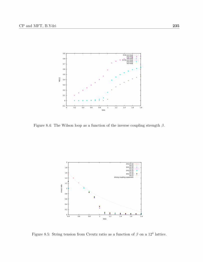
CP and MFT, B.Ydri 235
-0.1
0
0.1
0.2
0.3
0.4
0.5
0.6
0.7
0.8
0.9
0 0.2 0.4 0.6 0.8 1 1.2 1.4 1.6 1.8
W[I,
J]
beta
N=8,1x1 loop2x2 loop3x3 loop
N=10,1x1 loop2x2 loop3x3 loop
Figure 8.4: The Wilson loop as a function of the inverse coupling strength β.
0
0.2
0.4
0.6
0.8
1
1.2
1.4
1.6
1.8
2
0.4 0.6 0.8 1 1.2 1.4 1.6 1.8
creu
tz r
atio
beta
2X2,N=10N=12
3X3,N=10N=12
2X3,N=10N=10
3X2,N=10N=12
strong coupling expansion
Figure 8.5: String tension from Creutz ratio as a function of β on a 124 lattice.

Bibliography
[1] C. Gattringer and C. B. Lang, “Quantum chromodynamics on the lattice,” Lect.
Notes Phys. 788, 1 (2010).
[2] M. Creutz, “Quarks, Gluons And Lattices,” Cambridge, Uk: Univ. Pr. ( 1983) 169
P. ( Cambridge Monographs On Mathematical Physics).
[3] J. Smit, “Introduction to quantum fields on a lattice: A robust mate,” Cambridge
Lect. Notes Phys. 15, 1 (2002).
[4] H. J. Rothe, “Lattice gauge theories: An Introduction,” World Sci. Lect. Notes Phys.
74, 1 (2005).
[5] I. Montvay and G. Munster, “Quantum fields on a lattice,” Cambridge, UK: Univ.
Pr. (1994) 491 p. (Cambridge monographs on mathematical physics).

Chapter 9
Codes

File: /home/ydri/Desktop/TP_QFT/codes/metropolis-ym.f Page 1 of 6
program my_metropolis_ym implicit none integer dim,dimm,N,ther,mc,Tther,Tmc integer lambda,i,j,idum parameter (dimm=10,N=8) parameter (Tther=2**11,Tmc=2**11) double complex X(dimm,N,N) double precision xx,y,Accept,Reject,inn,interval,pa double precision act(Tmc),actio,average_act,error_act double precision t_1, t_2 real x0
call cpu_time(t_1) do dim=2,dimm if(dim.le.dimm)then c..........initialization of random number generator........... idum=-148175 x0=0.0 idum=idum-2*int(secnds(x0)) c.......inititialization of X................................ inn=1.0d0 do lambda=1,dimm if (lambda.le.dim)then do i=1,N do j=i,N if (j.ne.i) then xx=interval(idum,inn) y=interval(idum,inn) X(lambda,i,j)=cmplx(xx,y) X(lambda,j,i)=cmplx(xx,-y) else xx=interval(idum,inn) X(lambda,i,j)=xx endif enddo enddo else do i=1,N
do j=i,N if (j.ne.i) then xx=0.0d0 y=0.0d0 X(lambda,i,j)=cmplx(xx,y) X(lambda,j,i)=cmplx(xx,-y) else xx=0.0d0 X(lambda,i,j)=xx endif enddo enddo endif enddo c.... accepts including flips, rejects and the acceptance rate pa... Reject=0.0d0 Accept=0.0d0 pa=0.0d0 c.............thermalization....................................... do ther=1,Tther

File: /home/ydri/Desktop/TP_QFT/codes/metropolis-ym.f Page 2 of 6
call metropolis(dim,dimm,N,X,Reject,Accept,inn,idum) call adjust_inn(pa,inn,Reject,Accept) call action(dim,dimm,N,X,actio) write(*,*)ther,actio,pa write(10+dim,*)ther,actio,pa enddo c............monte carlo evolution................................. do mc=1,Tmc call metropolis(dim,dimm,N,X,Reject,Accept,inn,idum) call adjust_inn(pa,inn,Reject,Accept) call action(dim,dimm,N,X,actio) act(mc)=actio write(*,*)mc,act(mc),pa write(21+dim,*)mc,act(mc),pa enddo c.............measurements......................................... call jackknife_binning(Tmc,act,average_act,error_act) write(*,*)dim,average_act,error_act write(32,*)dim,average_act,error_act endif enddo c.........cpu time............................................ call cpu_time(t_2) write(*,*)"cpu_time", t_2-t_1 return end
c...............action...................................... subroutine action(dim,dimm,N,X,actio) implicit none integer dim,dimm,N,mu,nu,i,j,k,l double complex X(dimm,N,N) double precision actio,action0 actio=0.0d0
do mu =1,dimm do nu=mu+1,dimm action0=0.0d0 do i=1,N do j=1,N do k=1,N do l=1,N action0=action0+X(mu,i,j)*X(nu,j,k)*X(mu,k,l)*X(nu,l,i) & -X(mu,i,j)*X(mu,j,k)*X(nu,k,l)*X(nu,l,i) enddo enddo enddo enddo action0=-N*action0 actio=actio+action0 enddo enddo return end c..............metropolis algorithm.......................... subroutine metropolis(dim,dimm,N,X,Reject,Accept,inn,idum)
File: /home/ydri/Desktop/TP_QFT/codes/metropolis-ym.f Page 3 of 6
implicit none integer dim,dimm,N,i,j,lambda,idum double precision Reject,Accept,inn,interval,deltaS,ran2,z1,p1,xx,y double complex X(dimm,N,N),dc,dcbar do lambda=1,dim c..............diagonal.......................... do i=1,N xx=interval(idum,inn) y=interval(idum,inn) dc=cmplx(xx,0) dcbar=cmplx(xx,-0) call variationYM(dim,dimm,N,lambda,i,i,dc,dcbar,X,deltaS) if ( deltaS .gt. 0.0d0 ) then z1=ran2(idum) p1=dexp(-deltaS) if ( z1 .lt. p1 ) then X(lambda,i,i)=X(lambda,i,i)+dc+dcbar Accept=Accept+1.0d0 else Reject=Reject+1.0d0 endif else X(lambda,i,i)=X(lambda,i,i)+dc+dcbar Accept=Accept+1.0d0 endif enddoc............off diagonal.......................... do i=1,N do j=i+1,N xx=interval(idum,inn) y=interval(idum,inn) dc=cmplx(xx,y) dcbar=cmplx(xx,-y) call variationYM(dim,dimm,N,lambda,i,j,dc,dcbar,X,deltaS) if ( deltaS .gt. 0.0d0 ) then z1=ran2(idum) p1=dexp(-deltaS) if ( z1 .lt. p1 ) then X(lambda,i,j)=X(lambda,i,j)+dc Accept=Accept+1.0d0 else Reject=Reject+1.0d0
endif else X(lambda,i,j)=X(lambda,i,j)+dc Accept=Accept+1.0d0 endif X(lambda,j,i)=dconjg(X(lambda,i,j)) enddo enddo enddo return end c........variation of the action...........................
subroutine variationYM(dim,dimm,N,lambda,i,j,dc,dcbar,X,deltaS) implicit none integer dim,dimm,N,i,j,lambda,sigma,k,l,p,q double complex delta0,delta1,del2,del3,delta2 double precision delta11,delta22,deltaS double complex X(dimm,N,N),dc,dcbar delta0=0.0d0 do sigma=1,dim

File: /home/ydri/Desktop/TP_QFT/codes/metropolis-ym.f Page 4 of 6
if (sigma.ne.lambda)then do k=1,N delta0=delta0-X(sigma,i,k)*X(sigma,k,i) & -X(sigma,j,k)*X(sigma,k,j) enddo endif enddo delta1=0.0d0 delta1=delta1+dc*dcbar*delta0 if (i.eq.j) then delta1=delta1+0.5d0*(dc*dc+dcbar*dcbar)*delta0 endif do sigma=1,dim if (sigma.ne.lambda)then delta1=delta1+dc*dc*X(sigma,j,i)*X(sigma,j,i) & +dcbar*dcbar*X(sigma,i,j)*X(sigma,i,j) & +2.0d0*dc*dcbar*X(sigma,i,i)*X(sigma,j,j) endif enddo delta1=-N*delta1 delta11=real(delta1) del2=0.0d0 del3=0.0d0 do sigma=1,dim do k=1,N do l=1,N del2=del2+2.0d0*X(sigma,i,k)*X(lambda,k,l)*X(sigma,l,j) & -1.0d0*X(sigma,i,k)*X(sigma,k,l)*X(lambda,l,j) & -1.0d0*X(lambda,i,k)*X(sigma,k,l)*X(sigma,l,j) del3=del3+2.0d0*X(sigma,j,k)*X(lambda,k,l)*X(sigma,l,i) & -1.0d0*X(sigma,j,k)*X(sigma,k,l)*X(lambda,l,i) & -1.0d0*X(lambda,j,k)*X(sigma,k,l)*X(sigma,l,i) enddo enddo enddo delta2=0.0d0 delta2=-N*dcbar*del2-N*dc*del3 delta22=real(delta2) deltaS=delta11+delta22 return end c........the jackknife estimator................................ subroutine jackknife_binning(TMC,f,average,error) implicit none integer i,j,TMC,zbin,nbin double precision xm double precision f(1:TMC),sumf,y(1:TMC) double precision sig0,sig,error,average c..............TMC is the number of data points. sig0 is the standard deviation. sumf is the sum of all the data points f_i whereas xm is the average of f...... sig0=0.0d0 sumf=0.0d0 do i=1,TMC sumf=sumf+f(i) enddo xm=sumf/TMC c.... zbin is the number of elements we remove each time from the set of TMC data points. the minimum number we can remove is 1 whereas the maximum number we can remove is TMC-1.each time we remove zbin elements we end up with nbin sets (or bins)...........c do zbin=1,TMC-1 zbin=1 nbin=int(TMC/zbin) sig=0.0d0
File: /home/ydri/Desktop/TP_QFT/codes/metropolis-ym.f Page 5 of 6
do i=1,nbin,1c... y(i) is the average of the elements in the ith bin.This bin contains TMC-zbin data points after we had removed zbin elements. for zbin=1 we have nbin=TMC.In this case there are TMC bins and y_i=sum_j#ix_j/(TMC-1). for zbin=2 we have nbin=TMC/2. In this case there are TMC/2 bins and y_i= sum_jx_j/(TMC-2)-x_2i/(TMC-2)-x_2i-1/(TMC-2)... y(i)=sumf do j=1,zbin y(i)=y(i)-f((i-1)*zbin+j ) enddo y(i)= y(i)/(TMC-zbin)c..........the standard deviation computed for the ith bin.............. sig=sig+((nbin-1.0d0)/nbin)*(y(i)-xm)*(y(i)-xm) enddoc.... the standard deviation computed for the set of all bins with fixed zbin..... sig=sigc..................the error.................................... sig=dsqrt(sig)c.... we compare the result with the error obtained for the previous zbin, if it is larger, then this is the new value of the error... if (sig0 .lt. sig) sig0=sigc enddoc.... the final value of the error.............................................................. error=sig0 average=xm return end c.............the random number generator ran2.................. function ran2(idum) implicit none integer idum,IM1,IM2,IMM1,IA1,IA2,IQ1,IQ2,IR1,IR2,NTAB,NDIV real AM,EPS,RNMX double precision ran2 parameter (IM1=2147483563,IM2=2147483399,AM=1./IM1,IMM1=IM1-1, & IA1=40014,IA2=40692,IQ1=53668,IQ2=52774,IR1=12211, & IR2=3791,NTAB=32,NDIV=1+IMM1/NTAB,EPS=1.2E-7,RNMX=1.-EPS) integer idum2,j,k,iv(NTAB),iy SAVE iv,iy,idum2 DATA idum2/123456789/,iv/NTAB*0/,iy/0/ if (idum.le.0) then idum=max(-idum,1) idum2=idum do j=NTAB+8,1,-1 k=idum/IQ1 idum=IA1*(idum-k*IQ1)-k*IR1 if (idum.lt.0) idum=idum+IM1 if (j.le.NTAB) iv(j)=idum enddo iy=iv(1) endif k=idum/IQ1 idum=IA1*(idum-k*IQ1)-k*IR1 if (idum.lt.0) idum=idum+IM1 k=idum2/IQ2 idum2=IA2*(idum2-k*IQ2)-k*IR2 if (idum2.lt.0) idum2=idum2+IM2 j=1+iy/NDIV iy=iv(j)-idum2 iv(j)=idum if (iy.lt.1) iy=iy+IMM1 ran2=min(AM*iy,RNMX) return end
File: /home/ydri/Desktop/TP_QFT/codes/metropolis-ym.f Page 6 of 6
c.............interval.................................. function interval(idum,inn) implicit none double precision interval,inn,ran2 integer idum interval=ran2(idum) interval=interval+interval-1.0d0 interval=interval*inn return end c.........adjusting interval.............................. subroutine adjust_inn(pa,inn,Reject,Accept) implicit none double precision inn,pa,Reject,Accept c.....pa acceptance rate.................................. pa=(Accept)/(Reject+Accept)c........fixing the acceptance rate at 30 %.................. if (pa.ge.0.30) inn=inn*1.20d0 if (pa.le.0.25) inn=inn*0.80d0 return end
File: /home/ydri/Desktop/TP_QFT/codes/hybrid-ym.f Page 1 of 7
program my_hybrid_ym implicit none integer d,N,i,j,k,lambda,idum,tt,time,timeT,tther,Tth parameter (d=4,N=4) parameter (Tth=2**10) double precision gamma,mm,alpha,inn,dt,interval double complex X(d,N,N),P(d,N,N) double precision actio,ham,kin,variationH double precision Reject,Accept,pa double precision varH(Tth),varH_average,varH_error double precision ac(Tth),ac_average,ac_error real x0
c..........initialization of random number generator........... idum=-148175 x0=0.0c... seed should be set to a large odd integer according to the manual. secnds(x) gives number of seconds-x elapsed since midnight. the 2*int(secnds(x0)) is always even so seed is always odd.... idum=idum-2*int(secnds(x0)) c...................testing molecular dynamics...................... c call hot(N,d,idum,inn,X,P) c call cold(N,d,X)c time=1c dt=0.01d0c timeT=100c do tt=1,timeTc call molecular_dynamics(N,d,dt,time,gamma,mm,alpha,X,P)c call action(d,N,X,P,alpha,mm,gamma,actio,ham,kin)c write(9,*)tt,actio,hamc write(*,*)tt,actio,hamc enddo c.......parameters of molecular dynamics........... time=100 dt=0.01d0 c..................parameters.............. mm=0.0d0 alpha=0.0d0 do k=0,20 gamma=2.1d0-k*0.1d0 c............initialization of X and P............... inn=1.0d0 call hot(N,d,idum,inn,X,P) call cold(N,d,X) c................accepts including flips, rejects and the acceptance rate pa............... Reject=0.0d0 Accept=0.0d0 pa=0.0d0 c..............thermalization................ do tther=1,Tth call metropolis(N,d,gamma,mm,alpha,dt,time,X,P,Reject,Accept & ,variationH) enddo c..................monte carlo evolution....
File: /home/ydri/Desktop/TP_QFT/codes/hybrid-ym.f Page 2 of 7
do tther=1,Tth call metropolis(N,d,gamma,mm,alpha,dt,time,X,P,Reject,Accept & ,variationH) pa=(Accept)/(Reject+Accept) call action(d,N,X,P,alpha,mm,gamma,actio,ham,kin) ac(tther)=actio varH(tther)=dexp(-variationH) write(10,*)tther,actio,ham,kin,variationH,pa write(*,*)tther,actio,ham,kin,variationH,pa enddo c..............measurements................ call jackknife_binning(Tth,varH,varH_average,varH_error) write(*,*)gamma,alpha,mm,varH_average,varH_error write(11,*)gamma,alpha,mm,varH_average,varH_error call jackknife_binning(Tth,ac,ac_average,ac_error) write(*,*)gamma,alpha,mm,ac_average,ac_error write(12,*)gamma,alpha,mm,ac_average,ac_error enddo return end
c.................metropolis algorithm................ subroutine metropolis(N,d,gamma,mm,alpha,dt,time,X,P,Reject,Accept & ,variationH) implicit none integer N,d,i,j,mu,nu,k,l,idum,time double precision gamma,mm,alpha,inn,dt,ran2,Reject,Accept double complex var(d,N,N),X(d,N,N),X0(d,N,N),P(d,N,N),P0(d,N,N) double precision variations,variationH,probabilityS,probabilityH,r double precision actio,ham,kin
c........Gaussian initialization.....
call gaussian(d,N,P)
X0=X P0=P call action(d,N,X,P,alpha,mm,gamma,actio,ham,kin) variationS=actio variationH=ham
c............molecular dynamics evolution.....
call molecular_dynamics(N,d,dt,time,gamma,mm,alpha,X,P)
call action(d,N,X,P,alpha,mm,gamma,actio,ham,kin) variationS=actio-variationS variationH=ham-variationH
c........metropolis accept-reject step.................
if(variationH.lt.0.0d0)then accept=accept+1.0d0 else probabilityH=dexp(-variationH) r=ran2(idum) if (r.lt.probabilityH)then accept=accept+1.0d0 else X=X0 P=P0 Reject=Reject+1.0d0
File: /home/ydri/Desktop/TP_QFT/codes/hybrid-ym.f Page 3 of 7
endif endif return end
c...........actions and Hamiltonians......... subroutine action(d,N,X,P,alpha,mm,gamma,actio,ham,kin) implicit none integer d,N,mu,nu,i,j,k,l double complex X(d,N,N),P(d,N,N),ii,CS,action0,ham0,action1, & actio0,action2,ham1 double precision actio,ham,kin double precision mm,gamma,alpha ii=cmplx(0,1) actio0=cmplx(0,0) do mu =1,d do nu=mu+1,d action0=cmplx(0,0) do i=1,N do j=1,N do k=1,N do l=1,N action0=action0+X(mu,i,j)*X(nu,j,k)*X(mu,k,l)*X(nu,l,i) & -X(mu,i,j)*X(mu,j,k)*X(nu,k,l)*X(nu,l,i) enddo enddo enddo enddo actio0=actio0+action0 enddo enddo actio=real(actio0) actio=-N*gamma*actio ham1=cmplx(0,0) action2=cmplx(0,0) do mu =1,d ham0=cmplx(0,0) action1=cmplx(0,0) do i=1,N
do j=1,N ham0=ham0+P(mu,i,j)*P(mu,j,i) action1=action1+X(mu,i,j)*X(mu,j,i) enddo enddo action2=action2+action1 ham1=ham1+ham0 enddo ham=0.5d0*real(ham1) kin=ham actio=actio+0.5d0*mm*real(action2)
CS=0.0d0 do i=1,N do j=1,N do k=1,N CS=CS+ii*X(1,i,j)*X(2,j,k)*X(3,k,i) & -ii*X(1,i,j)*X(3,j,k)*X(2,k,i) enddo enddo enddo actio=actio+2.0d0*alpha*N*real(CS) ham=ham+actio
File: /home/ydri/Desktop/TP_QFT/codes/hybrid-ym.f Page 4 of 7
return end c.......the force............. subroutine variation(N,d,gamma,mm,alpha,X,var) implicit none integer N,d,i,j,mu,nu,k,l double precision gamma,mm,alpha double complex var(d,N,N),X(d,N,N),ii ii=dcmplx(0,1) do mu=1,d do i=1,N do j=i,N var(mu,i,j)=cmplx(0,0) do nu=1,d do k=1,N do l=1,N var(mu,i,j)=var(mu,i,j)+2.0d0*X(nu,j,k)*X(mu,k,l)*X(nu,l,i) & -X(nu,j,k)*X(nu,k,l)*X(mu,l,i) & -X(mu,j,k)*X(nu,k,l)*X(nu,l,i) enddo enddo enddo var(mu,i,j)=-N*gamma*var(mu,i,j)+mm*X(mu,j,i) if(mu.eq.1)then do k=1,N var(mu,i,j)=var(mu,i,j)+2.0d0*ii*alpha*N*X(2,j,k)*X(3,k,i) & -2.0d0*ii*alpha*N*X(3,j,k)*X(2,k,i) enddo endif if(mu.eq.2)then do k=1,N var(mu,i,j)=var(mu,i,j)+2.0d0*ii*alpha*N*X(3,j,k)*X(1,k,i) & -2.0d0*ii*alpha*N*X(1,j,k)*X(3,k,i) enddo endif if(mu.eq.3)then do k=1,N var(mu,i,j)=var(mu,i,j)+2.0d0*ii*alpha*N*X(1,j,k)*X(2,k,i) & -2.0d0*ii*alpha*N*X(2,j,k)*X(1,k,i) enddo
endif var(mu,j,i)=conjg(var(mu,i,j)) enddo enddo enddo return end c.............leap frog.............. subroutine molecular_dynamics(N,d,dt,time,gamma,mm,alpha,X,P) implicit none integer N,d,i,j,mu,nn,time double precision dt,gamma,mm,alpha double complex X(d,N,N),P(d,N,N),var(d,N,N) do nn=1,time call variation(N,d,gamma,mm,alpha,X,var) do mu=1,d do i=1,N do j=i,N P(mu,i,j)=P(mu,i,j)-0.5d0*dt*var(mu,i,j) X(mu,i,j)=X(mu,i,j)+dt*conjg(P(mu,i,j))
File: /home/ydri/Desktop/TP_QFT/codes/hybrid-ym.f Page 5 of 7
X(mu,j,i)=conjg(X(mu,i,j)) enddo enddo enddo call variation(N,d,gamma,mm,alpha,X,var) do mu=1,d do i=1,N do j=i,N P(mu,i,j)=P(mu,i,j)-0.5d0*dt*var(mu,i,j) P(mu,j,i)=conjg(P(mu,i,j)) enddo enddo enddo enddo return end c.........generation of Gaussian noise for the field P.................. subroutine gaussian(d,N,P) implicit none integer d,N,mu,i,j,idum double precision pi,phi,r,ran2 double complex ii,P(d,N,N) pi=dacos(-1.0d0) ii=cmplx(0,1) do mu=1,d do i=1,N phi=2.0d0*pi*ran2(idum) r=dsqrt(-2.0d0*dlog(1.0d0-ran2(idum))) P(mu,i,i)=r*dcos(phi) enddo do i=1,N do j=i+1,N phi=2.0d0*pi*ran2(idum) r=dsqrt(-1.0d0*dlog(1.0d0-ran2(idum))) P(mu,i,j)=r*dcos(phi)+ii*r*dsin(phi) P(mu,j,i)=conjg(P(mu,i,j)) enddo enddo enddo
return end
c........the jackknife estimator..................
subroutine jackknife_binning(TMC,f,average,error) implicit none integer i,j,TMC,zbin,nbin double precision xm double precision f(1:TMC),sumf,y(1:TMC) double precision sig0,sig,error,average sig0=0.0d0 sumf=0.0d0 do i=1,TMC sumf=sumf+f(i) enddo xm=sumf/TMC c do zbin=1,TMC-1 zbin=1 nbin=int(TMC/zbin) sig=0.0d0 do i=1,nbin,1

File: /home/ydri/Desktop/TP_QFT/codes/hybrid-ym.f Page 6 of 7
y(i)=sumf do j=1,zbin y(i)=y(i)-f((i-1)*zbin+j ) enddo y(i)= y(i)/(TMC-zbin) sig=sig+((nbin-1.0d0)/nbin)*(y(i)-xm)*(y(i)-xm) enddo sig=sig sig=dsqrt(sig) if (sig0 .lt. sig) sig0=sigc enddo error=sig0 average=xm return end c.............the random number generator ran2......... function ran2(idum) implicit none integer idum,IM1,IM2,IMM1,IA1,IA2,IQ1,IQ2,IR1,IR2,NTAB,NDIV real AM,EPS,RNMX double precision ran2 parameter (IM1=2147483563,IM2=2147483399,AM=1./IM1,IMM1=IM1-1, & IA1=40014,IA2=40692,IQ1=53668,IQ2=52774,IR1=12211, & IR2=3791,NTAB=32,NDIV=1+IMM1/NTAB,EPS=1.2E-7,RNMX=1.-EPS) integer idum2,j,k,iv(NTAB),iy SAVE iv,iy,idum2 DATA idum2/123456789/,iv/NTAB*0/,iy/0/ if (idum.le.0) then idum=max(-idum,1) idum2=idum do j=NTAB+8,1,-1 k=idum/IQ1 idum=IA1*(idum-k*IQ1)-k*IR1 if (idum.lt.0) idum=idum+IM1 if (j.le.NTAB) iv(j)=idum enddo iy=iv(1) endif k=idum/IQ1 idum=IA1*(idum-k*IQ1)-k*IR1 if (idum.lt.0) idum=idum+IM1 k=idum2/IQ2 idum2=IA2*(idum2-k*IQ2)-k*IR2 if (idum2.lt.0) idum2=idum2+IM2 j=1+iy/NDIV iy=iv(j)-idum2 iv(j)=idum if (iy.lt.1) iy=iy+IMM1 ran2=min(AM*iy,RNMX) return end
c........hot start................... subroutine hot(N,d,idum,inn,X,P) implicit none integer lambda,i,j,N,d,idum double complex X(d,N,N),P(d,N,N) double precision xx,y,inn,interval do lambda=1,d do i=1,N
File: /home/ydri/Desktop/TP_QFT/codes/hybrid-ym.f Page 7 of 7
do j=i,N if (j.ne.i) then xx=interval(idum,inn) y=interval(idum,inn) X(lambda,i,j)=cmplx(xx,y) X(lambda,j,i)=cmplx(xx,-y) xx=interval(idum,inn) y=interval(idum,inn) P(lambda,i,j)=cmplx(xx,y) P(lambda,j,i)=cmplx(xx,-y) else xx=interval(idum,inn) X(lambda,i,j)=xx xx=interval(idum,inn) P(lambda,i,j)=xx endif enddo enddo enddo return end c.............interval.............. function interval(idum,inn) implicit none double precision interval,inn,ran2 integer idum interval=ran2(idum) interval=interval+interval-1.0d0 interval=interval*inn return end c......cold start..................... subroutine cold(N,d,X) implicit none integer lambda,i,j,N,d double complex X(d,N,N)
do lambda=1,d do i=1,N do j=1,N X(lambda,i,j)=cmplx(0,0) enddo enddo enddo return end

File: /home/ydri/Desktop/TP_QFT/codes/hybrid-scalar-fuzzy.f Page 1 of 10
program my_hybrid_scalar_fuzzy implicit none integer N,i,j,k,idum,tt,time,tther,Tth,cou,ttco,Tco,Tmc,nn parameter (N=6) parameter (Tth=2**10,Tmc=2**10,Tco=2**0) double precision a,b,c,at,bt,ct double complex phi(N,N),P(N,N),phi0(N,N) double precision actio,ham,kin,quad,quar,mag,variationH,ev(1:N) double precision Reject,Accept,pa,inn,dt,interval,xx,y,t_1,t_2 double precision varH(Tmc),varH_average,varH_error double precision acti(Tmc),acti_average,acti_error double precision Cv(Tmc),Cv_average,Cv_error double precision ma(Tmc),ma_average,ma_error double precision chi(Tmc),chi_average,chi_error double precision p0(Tmc),p0_average,p0_error double precision pt(Tmc),pt_average,pt_error double precision kinet(Tmc),k_average,k_error double precision ide_average,ide_error double precision qu(Tmc),qu_average,qu_error double precision target_pa_high,target_pa_low,dt_max,dt_min,inc & ,dec real x0 call cpu_time(t_1) c..........initialization of random number generator........... idum=-148175 x0=0.0 idum=idum-2*int(secnds(x0)) c.............parameters.................. at=dsqrt(1.0d0*N)!1.0d0 a=at/dsqrt(1.0d0*N) ct=1.0d0 c=N*N*ct do k=0,0 bt=-5.0d0+k*0.1d0 b=N*dsqrt(1.0d0*N)*bt c.............initialization of phi and P.....
inn=1.0d0 call hot(N,idum,inn,phi,P) c.......parameters of molecular dynamics........... time=10 dt=0.01d0
c................accepts including flips, rejects and the acceptance rate pa............... Reject=0.0d0 Accept=0.0d0 pa=0.0d0 c.....the acceptance rate is fixed in [0.7,0.9] such that dt is in [0.0001,1].... target_pa_high=0.90d0 target_pa_low=0.70d0 dt_max=1.0d0 dt_min=0.0001d0 inc=1.2d0 dec=0.8d0 nn=1

File: /home/ydri/Desktop/TP_QFT/codes/hybrid-scalar-fuzzy.f Page 2 of 10
c............thermalization................................ do tther=1,Tth call metropolis(N,a,b,c,dt,time,phi,P,Reject,Accept & ,variationH,idum) call action(N,phi,P,a,b,c,kin,quad,quar,actio,ham,mag) cou=tther call adjust_inn(cou,pa,dt,time,Reject,Accept, & nn,target_pa_high,target_pa_low,dt_max,dt_min,inc,dec) write(*,*)tther,pa,dt,actio enddo c..................monte carlo evolution.................... do tther=1,Tmc
c................removing auto-correlations by separating data points by tco monte carlo steps.....
do ttco=1,Tco call metropolis(N,a,b,c,dt,time,phi,P,Reject,Accept & ,variationH,idum) enddo
c...........constructing thermalized obervables as vectors.......
call action(N,phi,P,a,b,c,kin,quad,quar,actio,ham,mag) acti(tther)=actio ma(tther)=mag p0(tther)=mag*mag/N**2 pt(tther)=quad/N kinet(tther)=kin qu(tther)=quar varH(tther)=dexp(-variationH) c...........adjusting the step dt.................
cou=tther call adjust_inn(cou,pa,dt,time,Reject,Accept, & nn,target_pa_high,target_pa_low,dt_max,dt_min,inc,dec) write(*,*)tther,pa,dt,actio
c.........the eigenvalues of phi...................................................
phi0=phi call eigenvalues(N,phi0,ev) write(62,*)tther,ev enddo c..............measurements................................................... c....................energy........................................................ call jackknife_binning(Tmc,acti,acti_average,acti_error) write(*,*)"action",a,bt,ct,acti_average,acti_error write(10,*)a,bt,ct,acti_average,acti_errorc.........specific heat Cv=<(S_i-<S>)^2>............................ do tther=1,Tmc Cv(tther)=0.0d0 Cv(tther)=Cv(tther)+acti(tther) Cv(tther)=Cv(tther)-acti_average Cv(tther)=Cv(tther)*Cv(tther) enddo call jackknife_binning(Tmc,Cv,Cv_average,Cv_error) write(*,*)"specific heat",a,bt,ct,Cv_average,Cv_error write(20,*)a,bt,ct,Cv_average,Cv_errorc..............magnetization................................................. call jackknife_binning(Tmc,ma,ma_average,ma_error) write(*,*)"magnetization",a,bt,ct,ma_average,ma_error

File: /home/ydri/Desktop/TP_QFT/codes/hybrid-scalar-fuzzy.f Page 3 of 10
write(30,*)a,bt,ct,ma_average,ma_errorc..............susceptibility........................................................... do tther=1,Tmc chi(tther)=0.0d0 chi(tther)=chi(tther)+ma(tther) chi(tther)=chi(tther)-ma_average chi(tther)=chi(tther)*chi(tther) enddo call jackknife_binning(Tmc,chi,chi_average,chi_error) write(*,*)"susceptibility", a,bt,ct,chi_average,chi_error write(40,*)a,bt,ct,chi_average,chi_errorc.............power in the zero mode............................................. call jackknife_binning(Tmc,p0,p0_average,p0_error) write(*,*)"zero power", a,bt,ct,p0_average,p0_error write(50,*)a,bt,ct,p0_average,p0_errorc.............total power=quadratic term/N......................................... call jackknife_binning(Tmc,pt,pt_average,pt_error) write(*,*)"total power=quadrtic/N",a,bt,ct,pt_average,pt_error write(60,*)a,bt,ct,pt_average,pt_errorc..............kinetic term......................................................... call jackknife_binning(Tmc,kinet,k_average,k_error) write(*,*)"kinetic",a,bt,ct,k_average,k_error write(70,*)a,bt,ct,k_average,k_errorc..............quartic term.... call jackknife_binning(Tmc,qu,qu_average,qu_error) write(*,*)"quartic", a,bt,ct,qu_average,qu_error write(80,*)a,bt,ct,qu_average,qu_errorc..............schwinger-dyson identity..................................... ide_average=2.0d0*a*k_average+2.0d0*b*N*pt_average & +4.0d0*c*qu_average ide_average=ide_average/(N*N) ide_error=2.0d0*a*k_error+2.0d0*b*N*pt_error & +4.0d0*c*qu_error ide_error=ide_error/(N*N) write(*,*)"ide", a,bt,ct,ide_average,ide_error write(81,*)a,bt,ct,ide_average,ide_errorc...............variation of hamiltonian................................. call jackknife_binning(Tmc,varH,varH_average,varH_error) write(*,*)"exp(-\Delta H)",a,bt,ct,varH_average,varH_error write(11,*)a,bt,ct,varH_average,varH_error enddo c.......................cpu time.............................................
call cpu_time(t_2) write(*,*)"cpu_time=", t_2-t_1 return end c.....................metropolis algorithm........................... subroutine metropolis(N,a,b,c,dt,time,phi,P,Reject,Accept & ,variationH,idum) implicit none integer N,i,j,mu,nu,k,l,idum,time double precision a,b,c,inn,dt,ran2,Reject,Accept double complex var(N,N),phi(N,N),phi0(N,N),P(N,N),P0(N,N) double precision variations,variationH,probabilityS,probabilityH,r double precision actio,ham,kin,quad,quar,mag c........Gaussian initialization, molecular dynamics evolution and variation of the Hamiltonian.... call gaussian(idum,N,P) phi0=phi P0=P call action(N,phi,P,a,b,c,kin,quad,quar,actio,ham,mag) variationS=actio variationH=ham

File: /home/ydri/Desktop/TP_QFT/codes/hybrid-scalar-fuzzy.f Page 4 of 10
call molecular_dynamics(N,dt,time,a,b,c,phi,P) call action(N,phi,P,a,b,c,kin,quad,quar,actio,ham,mag) variationS=actio-variationS variationH=ham-variationHc...........metropolis accept-reject step................. if(variationH.lt.0.0d0)then accept=accept+1.0d0 else probabilityH=dexp(-variationH) r=ran2(idum) if (r.lt.probabilityH)then accept=accept+1.0d0 else phi=phi0 P=P0 Reject=Reject+1.0d0 endif endif return end c....................eigenvalues............................ subroutine eigenvalues(N,phi0,ev) implicit none integer N,inf double complex cw(1:2*N-1) double precision rw(1:3*N-2) double complex phi0(1:N,1:N) double precision ev(1:N) c.....LAPACK's zheev diagonalizes hermitian matrices... call zheev('N','U',N,phi0,N,ev,cw,2*N-1,rw,inf) return end c................actions and Hamiltonians.................................. subroutine action(N,phi,P,a,b,c,kin,quad,quar,actio,ham,mag) implicit none integer N,mu,i,j,k,l
double complex phi(N,N),P(N,N) double precision a,b,c double precision kin,quad,quar,actio,ham,mag double complex kine,quadr,quart,ham0 double complex Lplus(1:N,1:N),Lminus(1:N,1:N),Lz(1:N,1:N) double complex X(1:3,1:N,1:N) c..................kinetic term and mass term.................. call SU2(N,X,Lplus,Lminus) kine=cmplx(0,0) do i=1,N do j=1,N do k=1,N do l=1,N kine=kine+X(1,i,j)*phi(j,k)*X(1,k,l)*phi(l,i) & +X(2,i,j)*phi(j,k)*X(2,k,l)*phi(l,i) & +X(3,i,j)*phi(j,k)*X(3,k,l)*phi(l,i) enddo enddo enddo enddo kin=-2.0d0*real(kine) quadr=cmplx(0,0) do i=1,N

File: /home/ydri/Desktop/TP_QFT/codes/hybrid-scalar-fuzzy.f Page 5 of 10
do j=1,N quadr=quadr+phi(i,j)*phi(j,i) enddo enddo kin=kin+0.5d0*(N*N-1.0d0)*real(quadr) quad=real(quadr)c.....................quartic term.......................... quart=cmplx(0,0) do i=1,N do j=1,N do k=1,N do l=1,N quart=quart+phi(i,j)*phi(j,k)*phi(k,l)*phi(l,i) enddo enddo enddo enddo quar=real(quart)c....................action........................... actio=a*kin+b*quad+c*quarc..................Hamiltonian............................... ham0=cmplx(0,0) do i=1,N do j=1,N ham0=ham0+P(i,j)*P(j,i) enddo enddo ham=0.5d0*real(ham0) ham=ham+actioc.......................magnetization............................. mag=0.0d0 do i=1,N mag=mag+phi(i,i) enddo mag=dabs(mag) return end c.................the force............................................. subroutine variation(N,a,b,c,phi,var) implicit none
integer N,i,j,k,l,nu doubleprecision a,b,c doublecomplex var(N,N),var1(N,N),phi(N,N) doublecomplex Lplus(1:N,1:N),Lminus(1:N,1:N),Lz(1:N,1:N) doublecomplex X(1:3,1:N,1:N) call SU2(N,X,Lplus,Lminus) do i=1,N do j=i,N var(i,j)=cmplx(0,0) do k=1,N do l=1,N var(i,j)=var(i,j)+X(1,j,k)*phi(k,l)*X(1,l,i) & +X(2,j,k)*phi(k,l)*X(2,l,i) & +X(3,j,k)*phi(k,l)*X(3,l,i) enddo enddo var1(i,j)=cmplx(0,0) do k=1,N do l=1,N var1(i,j)=var1(i,j)+phi(j,k)*phi(k,l)*phi(l,i) enddo enddo var(i,j)=-4.0d0*a*var(i,j)+(N*N-1.0d0)*a*phi(j,i)
File: /home/ydri/Desktop/TP_QFT/codes/hybrid-scalar-fuzzy.f Page 6 of 10
& +2.0d0*b*phi(j,i)+4.0d0*c*var1(i,j) var(j,i)=conjg(var(i,j)) enddo enddo return end c..........SU(2) generators.................... subroutine SU2(N,L,Lplus,Lminus) implicit none integer i,j,N double complex Lplus(1:N,1:N),Lminus(1:N,1:N),Lz(1:N,1:N) double complex L(1:3,1:N,1:N) double complex ii ii=cmplx(0,1) do i=1,N do j=1,N if( ( i + 1 ) .eq. j )then Lplus(i,j) =dsqrt( ( N - i )*i*1.0d0 ) else Lplus(i,j)=0.0d0 endif if( ( i - 1 ) .eq. j )then Lminus(i,j)=dsqrt( ( N - j )*j*1.0d0 ) else Lminus(i,j)=0.0d0 endif if( i.eq.j)then Lz(i,j) = ( N + 1 - i - i )/2.0d0 else Lz(i,j) = 0.0d0 endif L(1,i,j)=0.50d0*(Lplus(i,j)+Lminus(i,j)) L(2,i,j)=-0.50d0*ii*(Lplus(i,j)-Lminus(i,j)) L(3,i,j)=Lz(i,j) enddo enddo return end
c..............leap frog...................................... subroutine molecular_dynamics(N,dt,time,a,b,c,phi,P) implicit none integer N,i,j,nn,time double precision dt,a,b,c double complex phi(N,N),P(N,N),var(N,N),ii ii=cmplx(0,1) do nn=1,time call variation(N,a,b,c,phi,var) do i=1,N do j=i,N if (j.ne.i)then P(i,j)=P(i,j)-0.5d0*dt*var(i,j) phi(i,j)=phi(i,j)+dt*conjg(P(i,j)) phi(j,i)=conjg(phi(i,j)) else P(i,i)=P(i,i)-0.5d0*dt*var(i,i) phi(i,i)=phi(i,i)+dt*conjg(P(i,i)) phi(i,i)=phi(i,i)-ii*aimag(phi(1,1)) endif enddo

File: /home/ydri/Desktop/TP_QFT/codes/hybrid-scalar-fuzzy.f Page 7 of 10
enddo c...........last step of leap frog....................................... call variation(N,a,b,c,phi,var) do i=1,N do j=i,N if(j.ne.i)then P(i,j)=P(i,j)-0.5d0*dt*var(i,j) P(j,i)=conjg(P(i,j)) else P(i,i)=P(i,i)-0.5d0*dt*var(i,i) P(i,i)=P(i,i)-ii*aimag(P(i,i)) endif enddo enddo enddo return end c.........generation of Gaussian noise for the field P.................. subroutine gaussian(idum,N,P) implicit none integer N,mu,i,j,idum double precision pi,phi,r,ran2 double complex ii,P(N,N) pi=dacos(-1.0d0) ii=cmplx(0,1) do i=1,N phi=2.0d0*pi*ran2(idum) r=dsqrt(-2.0d0*dlog(1.0d0-ran2(idum))) P(i,i)=r*dcos(phi) enddo do i=1,N do j=i+1,N phi=2.0d0*pi*ran2(idum) r=dsqrt(-1.0d0*dlog(1.0d0-ran2(idum))) P(i,j)=r*dcos(phi)+ii*r*dsin(phi) P(j,i)=conjg(P(i,j)) enddo enddo
return end
c........the jackknife estimator.................. subroutine jackknife_binning(TMC,f,average,error) implicit none integer i,j,TMC,zbin,nbin double precision xm double precision f(1:TMC),sumf,y(1:TMC) double precision sig0,sig,error,average sig0=0.0d0 sumf=0.0d0 do i=1,TMC sumf=sumf+f(i) enddo xm=sumf/TMC c do zbin=1,TMC-1 zbin=1 nbin=int(TMC/zbin) sig=0.0d0 do i=1,nbin,1 y(i)=sumf

File: /home/ydri/Desktop/TP_QFT/codes/hybrid-scalar-fuzzy.f Page 8 of 10
do j=1,zbin y(i)=y(i)-f((i-1)*zbin+j ) enddo y(i)= y(i)/(TMC-zbin) sig=sig+((nbin-1.0d0)/nbin)*(y(i)-xm)*(y(i)-xm) enddo sig=sig sig=dsqrt(sig) if (sig0 .lt. sig) sig0=sigc enddo error=sig0 average=xm return end c.............the random number generator ran2......... function ran2(idum) implicit none integer idum,IM1,IM2,IMM1,IA1,IA2,IQ1,IQ2,IR1,IR2,NTAB,NDIV real AM,EPS,RNMX double precision ran2 parameter (IM1=2147483563,IM2=2147483399,AM=1./IM1,IMM1=IM1-1, & IA1=40014,IA2=40692,IQ1=53668,IQ2=52774,IR1=12211, & IR2=3791,NTAB=32,NDIV=1+IMM1/NTAB,EPS=1.2E-7,RNMX=1.-EPS) integer idum2,j,k,iv(NTAB),iy SAVE iv,iy,idum2 DATA idum2/123456789/,iv/NTAB*0/,iy/0/ if (idum.le.0) then idum=max(-idum,1) idum2=idum do j=NTAB+8,1,-1 k=idum/IQ1 idum=IA1*(idum-k*IQ1)-k*IR1 if (idum.lt.0) idum=idum+IM1 if (j.le.NTAB) iv(j)=idum enddo iy=iv(1) endif k=idum/IQ1 idum=IA1*(idum-k*IQ1)-k*IR1
if (idum.lt.0) idum=idum+IM1 k=idum2/IQ2 idum2=IA2*(idum2-k*IQ2)-k*IR2 if (idum2.lt.0) idum2=idum2+IM2 j=1+iy/NDIV iy=iv(j)-idum2 iv(j)=idum if (iy.lt.1) iy=iy+IMM1 ran2=min(AM*iy,RNMX) return end
c........hot start................... subroutine hot(N,idum,inn,phi,P) implicit none integer lambda,i,j,N,d,idum double complex phi(N,N),P(N,N) double precision xx,y,inn,interval do i=1,N do j=i,N if (j.ne.i) then
File: /home/ydri/Desktop/TP_QFT/codes/hybrid-scalar-fuzzy.f Page 9 of 10
xx=interval(idum,inn) y=interval(idum,inn) phi(i,j)=cmplx(xx,y) phi(j,i)=cmplx(xx,-y) xx=interval(idum,inn) y=interval(idum,inn) P(i,j)=cmplx(xx,y) P(j,i)=cmplx(xx,-y) else xx=interval(idum,inn) phi(i,j)=xx xx=interval(idum,inn) P(i,j)=xx endif enddo enddo return end c.............interval.............. function interval(idum,inn) implicit none double precision interval,inn,ran2 integer idum interval=ran2(idum) interval=interval+interval-1.0d0 interval=interval*inn return end c......cold start..................... subroutine cold(N,phi) implicit none integer lambda,i,j,N double complex phi(N,N) do i=1,N do j=1,N phi(i,j)=cmplx(0,0) enddo enddo return end c.........adjusting interval.................. subroutine adjust_inn(cou,pa,dt,time,Rejec,Accept, & nn,target_pa_high,target_pa_low,dt_max,dt_min,inc,dec) implicit none double precision dt,pa,Rejec,Accept integer time,cou,cou1 integer nn double precision target_pa_high,target_pa_low,dt_max,dt_min,inc, & dec,rho1,rho2,dtnew c.....pa acceptance rate............ pa=(Accept)/(Rejec+Accept) cou1=mod(cou,nn) if (cou1.eq.0)thenc........fixing the acceptance rate between 90 % 70 %.................. if (pa.ge.target_pa_high) then

File: /home/ydri/Desktop/TP_QFT/codes/hybrid-scalar-fuzzy.f Page 10 of 10
dtnew=dt*inc if (dtnew.le.dt_max)then dt=dtnew else dt=dt_max endif endif if (pa.le.target_pa_low) then dtnew=dt*dec if (dtnew.ge.dt_min)then dt=dtnew else dt=dt_min endif endif endif return end

File: /home/ydri/Desktop/TP_QFT/codes/phi-four-on-lattice.f Page 1 of 7
program my_phi_four_on_lattice implicit none integer N,idum,time,cou,nn,kk,ith,imc,ico,Tth,Tmc,Tco parameter (N=16) parameter (Tth=2**13,Tmc=2**14,Tco=2**3) double precision dt,kappa,g,phi(N,N),P(N,N),lambda_l,mu0_sq_l double precision mass,linear,kinetic,potential,act,Ham,variationH, & quartic double precision target_pa_high,target_pa_low,dt_max,dt_min,inc & ,dec,inn,pa,accept,reject real x0 double precision ac(Tmc),ac_average,ac_error,cv(Tmc),cv_average, & cv_error,lin(Tmc),lin_average,lin_error,susc(Tmc),susc_average, & susc_error,ac2(Tmc),ac2_av,ac2_er,ac4(Tmc),ac4_av,ac4_er,binder, & binder_e c..........initialization of random number generator........... idum=-148175 x0=0.0 idum=idum-2*int(secnds(x0)) c.............parameters.................. lambda_l=0.5d0 do kk=0,15 mu0_sq_l=-1.5d0+kk*0.1d0 kappa=dsqrt(8.0d0*lambda_l+(4.0d0+mu0_sq_l)*(4.0d0+mu0_sq_l)) kappa=kappa/(4.0d0*lambda_l) kappa=kappa-(4.0d0+mu0_sq_l)/(4.0d0*lambda_l) g=kappa*kappa*lambda_l c.............initialization of phi and P..... inn=1.0d0 call hot(N,idum,inn,phi,P) c.......parameters of molecular dynamics........... time=10 dt=0.01d0 c................accepts including flips, rejects and the acceptance rate pa...............
Reject=0.0d0 Accept=0.0d0 pa=0.0d0 c.....the acceptance rate is fixed in [0.7,0.9] such that dt is in [0.0001,1].... target_pa_high=0.90d0 target_pa_low=0.70d0 dt_max=1.0d0 dt_min=0.0001d0 inc=1.2d0 dec=0.8d0 nn=1 c...............thermalization...... do ith=1,Tth call metropolis(time,dt,N,kappa,g,idum,accept,reject, & variationH,P,phi) call adjust_inn(cou,pa,dt,time,Reject,Accept, & nn,target_pa_high,target_pa_low,dt_max,dt_min,inc,dec) call action(N,kappa,g,P,phi,mass,linear,kinetic,potential, & act,Ham,quartic)

File: /home/ydri/Desktop/TP_QFT/codes/phi-four-on-lattice.f Page 2 of 7
write(9+kk,*) ith,act,Ham,variationH,pa,dt enddo c..........Monte Carlo evolution..... do imc=1,Tmc do ico=1,Tco call metropolis(time,dt,N,kappa,g,idum,accept,reject, & variationH,P,phi) call adjust_inn(cou,pa,dt,time,Reject,Accept, & nn,target_pa_high,target_pa_low,dt_max,dt_min,inc,dec) enddo call action(N,kappa,g,P,phi,mass,linear,kinetic,potential, & act,Ham,quartic) ac(imc)=act lin(imc)=dabs(linear) ac2(imc)=linear*linear ac4(imc)=linear*linear*linear*linear write(9+kk,*) imc+Tth,act,Ham,variationH,pa,dt enddo
c....................observables........................ c.................action.................................. call jackknife_binning(Tmc,ac,ac_average,ac_error) write(50,*)mu0_sq_l,lambda_l,kappa,g,ac_average,ac_errorc.................specific heat.................................. do imc=1,Tmc cv(imc)=ac(imc)-ac_average cv(imc)=cv(imc)**(2.0d0) enddo call jackknife_binning(Tmc,cv,cv_average,cv_error) write(60,*)mu0_sq_l,lambda_l,kappa,g,cv_average,cv_errorc...............magnetization.................................... call jackknife_binning(Tmc,lin,lin_average,lin_error) write(70,*)mu0_sq_l,lambda_l,kappa,g,lin_average,lin_errorc...............susceptibility............................... do imc=1,Tmc susc(imc)=lin(imc)-lin_average susc(imc)=susc(imc)**(2.0d0) enddo call jackknife_binning(Tmc,susc,susc_average,susc_error) write(80,*)mu0_sq_l,lambda_l,kappa,g,susc_average,susc_errorc...............Binder cumulant........................... call jackknife_binning(Tmc,ac2,ac2_av,ac2_er) write(81,*)mu0_sq_l,lambda_l,kappa,g,ac2_av,ac2_er call jackknife_binning(Tmc,ac4,ac4_av,ac4_er) write(82,*)mu0_sq_l,lambda_l,kappa,g,ac4_av,ac4_er binder=1.0d0-ac4_av/(3.0d0*ac2_av*ac2_av) binder_e=-ac4_er/(3.0d0*ac2_av*ac2_av) & +2.0d0*ac4_av*ac2_er/(3.0d0*ac2_av*ac2_av*ac2_av) write(90,*)mu0_sq_l,lambda_l,kappa,g,binder,binder_e enddo return end subroutine metropolis(time,dt,N,kappa,g,idum,accept,reject, & variationH,P,phi) implicit none integer time,N,idum double precision dt,kappa,g,accept,reject,P(N,N),phi(N,N), & variationH,P0(N,N),phi0(N,N),r,ran2,probability double precision mass,linear,kinetic,potential,act,Ham,quartic call gaussian(N,idum,P) P0=P

File: /home/ydri/Desktop/TP_QFT/codes/phi-four-on-lattice.f Page 3 of 7
phi0=phi call action(N,kappa,g,P,phi,mass,linear,kinetic,potential,act,Ham, & quartic) variationH=-Ham call leap_frog(time,dt,N,kappa,g,P,phi) call action(N,kappa,g,P,phi,mass,linear,kinetic,potential,act,Ham, & quartic) variationH=variationH+Ham if (variationH.lt.0.0d0)then accept=accept+1.0d0 else probability=dexp(-variationH) r=ran2(idum) if (r.lt.probability)then accept=accept+1.0d0 else P=P0 phi=phi0 reject=reject+1.0d0 endif endif return end subroutine gaussian(N,idum,P) implicit none integer N,i,j,idum double precision P(N,N),ph,r,pi,ran2 pi=dacos(-1.0d0) do i=1,N do j=1,N r=dsqrt(-2.0d0*dlog(1.0d0-ran2(idum))) ph=2.0d0*pi*ran2(idum) P(i,j)=r*dcos(ph) enddo enddo return end
subroutine leap_frog(time,dt,N,kappa,g,P,phi) implicit none integer time,N,nn,i,j double precision kappa,g,phi(N,N),P(N,N),force(N,N),dt do nn=1,time call scalar_force(N,phi,kappa,g,force) do i=1,N do j=1,N P(i,j)=P(i,j)-0.5d0*dt*force(i,j) phi(i,j)=phi(i,j)+dt*P(i,j) enddo enddo call scalar_force(N,phi,kappa,g,force) do i=1,N do j=1,N P(i,j)=P(i,j)-0.5d0*dt*force(i,j) enddo enddo enddo return end

File: /home/ydri/Desktop/TP_QFT/codes/phi-four-on-lattice.f Page 4 of 7
subroutine scalar_force(N,phi,kappa,g,force) implicit none integer N,i,j,ip(N),im(N) double precision phi(N,N),kappa,g,force(N,N) double precision force1,force2,force3 call ipp(N,ip) call imm(N,im) do i=1,N do j=1,N force1=phi(ip(i),j)+phi(im(i),j)+phi(i,ip(j))+phi(i,im(j)) force1=-2.0d0*kappa*force1 force2=2.0d0*phi(i,j) force3=phi(i,j)*(phi(i,j)*phi(i,j)-1.0d0) force3=4.0d0*g*force3 force(i,j)=force1+force2+force3 enddo enddo return end
subroutine action(N,kappa,g,P,phi,mass,linear,kinetic,potential, & act,Ham,quartic) implicit none integer N,i,j,ip(N) double precision kappa,g double precision phi(N,N),P(N,N),act,potential,mass,kinetic, & kineticH,ham,linear,quartic call ipp(N,ip) kinetic=0.0d0 mass=0.0d0 kineticH=0.0d0 potential=0.0d0 linear=0.0d0 quartic=0.0d0 do i=1,N do j=1,N linear=linear+phi(i,j) quartic=quartic+phi(i,j)*phi(i,j)*phi(i,j)*phi(i,j) kinetic=kinetic+phi(i,j)*(phi(ip(i),j)+phi(i,ip(j))) mass=mass+phi(i,j)*phi(i,j) potential=potential & +(phi(i,j)*phi(i,j)-1.0d0)*(phi(i,j)*phi(i,j)-1.0d0) kineticH=kineticH+P(i,j)*P(i,j) enddo enddo kinetic=-2.0d0*kappa*kinetic potential=g*potential act=kinetic+mass+potential kineticH=0.5d0*kineticH ham=kineticH+act return end subroutine ipp(N,ip) implicit none integer ip(N),i,N do i=1,N-1 ip(i)=i+1 enddo ip(N)=1

File: /home/ydri/Desktop/TP_QFT/codes/phi-four-on-lattice.f Page 5 of 7
return end subroutine imm(N,im) implicit none integer im(N),i,N do i=2,N im(i)=i-1 enddo im(1)=N return end
c........the jackknife estimator..................
subroutine jackknife_binning(TMC,f,average,error) implicit none integer i,j,TMC,zbin,nbin double precision xm double precision f(1:TMC),sumf,y(1:TMC) double precision sig0,sig,error,average sig0=0.0d0 sumf=0.0d0 do i=1,TMC sumf=sumf+f(i) enddo xm=sumf/TMC c do zbin=1,TMC-1 zbin=1 nbin=int(TMC/zbin) sig=0.0d0 do i=1,nbin,1 y(i)=sumf do j=1,zbin y(i)=y(i)-f((i-1)*zbin+j ) enddo y(i)= y(i)/(TMC-zbin) sig=sig+((nbin-1.0d0)/nbin)*(y(i)-xm)*(y(i)-xm) enddo sig=sig sig=dsqrt(sig) if (sig0 .lt. sig) sig0=sigc enddo error=sig0 average=xm return end c.............the random number generator ran2......... function ran2(idum) implicit none integer idum,IM1,IM2,IMM1,IA1,IA2,IQ1,IQ2,IR1,IR2,NTAB,NDIV real AM,EPS,RNMX double precision ran2 parameter (IM1=2147483563,IM2=2147483399,AM=1./IM1,IMM1=IM1-1, & IA1=40014,IA2=40692,IQ1=53668,IQ2=52774,IR1=12211, & IR2=3791,NTAB=32,NDIV=1+IMM1/NTAB,EPS=1.2E-7,RNMX=1.-EPS) integer idum2,j,k,iv(NTAB),iy SAVE iv,iy,idum2 DATA idum2/123456789/,iv/NTAB*0/,iy/0/ if (idum.le.0) then

File: /home/ydri/Desktop/TP_QFT/codes/phi-four-on-lattice.f Page 6 of 7
idum=max(-idum,1) idum2=idum do j=NTAB+8,1,-1 k=idum/IQ1 idum=IA1*(idum-k*IQ1)-k*IR1 if (idum.lt.0) idum=idum+IM1 if (j.le.NTAB) iv(j)=idum enddo iy=iv(1) endif k=idum/IQ1 idum=IA1*(idum-k*IQ1)-k*IR1 if (idum.lt.0) idum=idum+IM1 k=idum2/IQ2 idum2=IA2*(idum2-k*IQ2)-k*IR2 if (idum2.lt.0) idum2=idum2+IM2 j=1+iy/NDIV iy=iv(j)-idum2 iv(j)=idum if (iy.lt.1) iy=iy+IMM1 ran2=min(AM*iy,RNMX) return end
c........hot start................... subroutine hot(N,idum,inn,phi,P) implicit none integer lambda,i,j,N,idum double precision phi(N,N),P(N,N) double precision inn,interval do i=1,N do j=1,N phi(i,j)=interval(idum,inn) P(i,j)=interval(idum,inn) enddo enddo return end
c.........adjusting interval.................. subroutine adjust_inn(cou,pa,dt,time,Reject,Accept, & nn,target_pa_high,target_pa_low,dt_max,dt_min,inc,dec) implicit none double precision dt,pa,Reject,Accept integer time,cou,cou1 integer nn double precision target_pa_high,target_pa_low,dt_max,dt_min,inc, & dec,rho1,rho2,dtnew c.....pa acceptance rate............ pa=(Accept)/(Reject+Accept) cou1=mod(cou,nn) if (cou1.eq.0)thenc........fixing the acceptance rate between 90 % 70 %.................. if (pa.ge.target_pa_high) then dtnew=dt*inc if (dtnew.le.dt_max)then dt=dtnew else dt=dt_max endif endif
File: /home/ydri/Desktop/TP_QFT/codes/phi-four-on-lattice.f Page 7 of 7
if (pa.le.target_pa_low) then dtnew=dt*dec if (dtnew.ge.dt_min)then dt=dtnew else dt=dt_min endif endif endif return end c.............interval.............. function interval(idum,inn) implicit none double precision interval,inn,ran2 integer idum interval=ran2(idum) interval=interval+interval-1.0d0 interval=interval*inn return end
File: /home/ydri/Desktop/TP_QFT/cod…metropolis-scalar-multitrace.f Page 1 of 7
program my_metropolis_scalar_multitrace implicit none integer N,i,k,idum,ither,Tther,imont,ico,tmo,Tmont,Tco,counter, & Pow1,Pow2,Pow3 parameter (N=10) parameter (pow1=20,pow2=20,pow3=5) parameter (Tther=2**pow1,Tmont=2**pow2,Tco=2**pow3) double precision a,b,c,d,g,at,bt,ct,eta,v22,v41,v21,ap,bp,cp,dp,e, & ep,fp double precision ran2,inn,interval,accept,reject,pa,t_1,t_2 double precision lambda(N) double precision actio,actio0,sum1,sum2,sum4,sumv,actio1,actio2, & actio4 double precision ac(Tmont),ac_average,ac_error double precision id,ide(Tmont),ide_average,ide_error double precision cv(Tmont),cv_average,cv_error double precision va(Tmont),va_average,va_error double precision p0(Tmont),p0_average,p0_error double precision pt(Tmont),pt_average,pt_error double precision p4(Tmont),p4_average,p4_error double precision su(Tmont),su_average,su_error double precision sus(Tmont),sus_average,sus_error real x0 call cpu_time(t_1) c...........initialization of the random number generator........ idum=-148175 x0=0.0 idum=idum-2*int(secnds(x0)) c............parameters of the model.................. c............kinetic parameter:the pure quartic matrix model is obtained by setting at=0............ at=1.0d0 a=at/dsqrt(1.0d0*N)c.........Seamann's values.................. v21=-1.0d0 v22=0.0d0 v41=1.5d0c.........Ydri's proposal....................c v21=1.0d0c v22=1.0d0/8.0d0c v41=0.0d0c...........principal multitrace coupling........................ eta=v22-0.75d0*v41 d=-2.0d0*eta*at*at*N d=d/3.0d0 e=dc..........further multitrace couplings (odd terms)................. ap=4.0d0*at*at*v22/3.0d0 dp=-2.0d0*at*at*v22/3.0d0 dp=dp/N cp=-2.0d0*at*at*N*v41/3.0d0 bp=-at*dsqrt(1.0d0*N)*v21/2.0d0 c.......ep and fp are included in c and b respectively.... ep=at*at*N*N*v41/6.0d0 fp=at*N*dsqrt(1.0d0*N)*v21/2.0d0c............quartic parameter: here c is C=c+ep of note.......................... ct=1.0d0 c=N*N*ctc...........mass parameter: here b is B=b+fp of note................... do k=0,0 bt=-5.0d0+k*0.1d0 b=N*dsqrt(1.0d0*N)*btc......the parameters b and c in terms of g: the single parameter of the quartic matrix model........

File: /home/ydri/Desktop/TP_QFT/cod…metropolis-scalar-multitrace.f Page 2 of 7
c g=1.0d0c b=-N/gc c=N c c=c/(4.0d0*g) c...................initialization of the eigenvalues... inn=1.0d0 do i=1,N lambda(i)=interval(idum,inn) enddo c................accepts including flips, rejects and the acceptance rate pa............... Reject=0.0d0 Accept=0.0d0 pa=0.0d0 c.........thermalization......................................................... do ither=1,Tther call standard_metropolis(N,ap,b,bp,c,cp,d,dp,ep,fp,lambda, & accept,reject,idum,inn,pa) call action(N,ap,b,bp,c,cp,d,dp,ep,fp,lambda,actio,actio0, & sum1,sum2,sum4,sumv,id,actio1,actio2,actio4) write(*,*)ither,actio0,actio,dabs(sum1),sum2,sum4,id,pa,inn write(7,*)ither,actio0,actio,dabs(sum1),sum2,sum4,sumv,id & ,pa,inn enddo c.......monte carlo evolution.................. counter=0 do imont=1,Tmont c........removing auto-correlations by separating data points by tco monte carlo setps................
do ico=1,Tco call standard_metropolis(N,ap,b,bp,c,cp,d,dp,ep,fp,lambda & ,accept,reject,idum,inn,pa) enddo
c..........construction of thermalized observables......................................
call action(N,ap,b,bp,c,cp,d,dp,ep,fp,lambda,actio,actio0, & sum1,sum2,sum4,sumv,id,actio1,actio2,actio4) c if ((id.ge.0.8d0).and.(id.le.1.2d0))then counter=counter+1 ac(counter)=actio0+actio1 ide(counter)=id va(counter)=sumv su(counter)=dabs(sum1) p0(counter)=sum1*sum1/(N*N) pt(counter)=sum2/N p4(counter)=sum4 write(*,*)imont,counter,sum2,sum4,id write(8,*)imont,counter,sum2,sum4,id
c....................eigenvalues........................
write(150+k,*)counter,lambdac endif enddo c...............measurements............ Tmo=counterc................action and vandermonde................... call jackknife_binning(Tmo,ac,ac_average,ac_error)

File: /home/ydri/Desktop/TP_QFT/cod…metropolis-scalar-multitrace.f Page 3 of 7
write(10,*)bt,ct,d,ac_average,ac_error call jackknife_binning(Tmo,va,va_average,va_error) write(11,*)bt,ct,d,va_average,va_errorc..................identity................. call jackknife_binning(Tmo,ide,ide_average,ide_error) write(12,*)bt,ct,d,ide_average,ide_error write(*,*)bt,ct,d,ide_average,ide_error, "identity"c............power in zero modes, total power and quartic term............. call jackknife_binning(Tmo,p0,p0_average,p0_error) write(13,*)bt,ct,d,p0_average,p0_error call jackknife_binning(Tmo,pt,pt_average,pt_error) write(14,*)bt,ct,d,pt_average,pt_error write(*,*)bt,ct,d,pt_average,pt_error, "total power" call jackknife_binning(Tmo,p4,p4_average,p4_error) write(15,*)bt,ct,d,p4_average,p4_errorc.......magnetization and susceptibility.............. call jackknife_binning(Tmo,su,su_average,su_error) write(16,*)bt,ct,d,su_average,su_error do i=1,Tmo sus(i)= (su(i)-su_average)*(su(i)-su_average) enddo call jackknife_binning(Tmo,sus,sus_average,sus_error) write(17,*)bt,ct,d,sus_average,sus_error c..................specific heat.................... do i=1,Tmo cv(i)=(ac(i)-ac_average)**2 enddo call jackknife_binning(Tmo,cv,cv_average,cv_error) write(20,*)bt,ct,d,cv_average,cv_error enddo c..........cpu time and detail of simulation....................... call cpu_time(t_2) write(99,*)N,d,bt,ct,tmont,tmo,tco,tther,t_2-t_1 return end c.............metropolis algorithm........................... subroutine standard_metropolis(N,ap,b,bp,c,cp,d,dp,ep,fp,lambda & ,accept,reject,idum,inn,pa) implicit none
integer N,i,idum double precision lambda(N),var,pro,r,b,c,d,accept,reject,ran2, & h,inn,interval,pa,ap,bp,cp,dp,ep,fp do i=1,Nc...........variation of the action.................... h=interval(idum,inn) call variation(N,ap,b,bp,c,cp,d,dp,ep,fp,i,h,lambda,Var)c............metropolis accept-reject step.......................... if(var.gt.0.0d0)then pro=dexp(-var) r=ran2(idum) if (r.lt.pro) then lambda(i)=lambda(i)+h accept=accept+1.0d0 else reject=reject+1.0d0 endif else lambda(i)=lambda(i)+h accept=accept+1.0d0 endif enddo c............adjusting the interval inn................

File: /home/ydri/Desktop/TP_QFT/cod…metropolis-scalar-multitrace.f Page 4 of 7
call adjust_inn(pa,inn,Reject,Accept) return end
c.....................variation of the action............ subroutine variation(N,ap,b,bp,c,cp,d,dp,ep,fp,i,h,lambda,Var) implicit none integer N,i,k double precision lambda(N),var,b,c,d,h,ap,bp,cp,dp,ep,fp double precision dsum2,dsum4,sum2,dvand,dd,dvande double precision sum1,sum3,var1,var2,var3,var4 dsum2=h*h+2.0d0*h*lambda(i) dsum4=6.0d0*h*h*lambda(i)*lambda(i) & +4.0d0*h*lambda(i)*lambda(i)*lambda(i)+4.0d0*h*h*h*lambda(i) & +h*h*h*h sum3=0.0d0 sum2=0.0d0 sum1=0.0d0 do k=1,N sum3=sum3+lambda(k)*lambda(k)*lambda(k) sum2=sum2+lambda(k)*lambda(k) sum1=sum1+lambda(k) enddo dvand=0.0d0 do k=i+1,N dd=1.0d0 dd=dd+h/(lambda(i)-lambda(k)) dd=dabs(dd) dvand=dvand+dlog(dd) enddo dvand=-dvand dvande=0.0d0 do k=1,i-1 dd=1.0d0 dd=dd+h/(lambda(i)-lambda(k)) dd=dabs(dd) dvande=dvande+dlog(dd) enddo dvande=-dvande dvand=dvand+dvande dvand=2.0d0*dvand var=b*dsum2+c*dsum4+2.0d0*d*dsum2*sum2+d*dsum2*dsum2+dvand var1=h*h+2.0d0*h*sum1 var4=var1*var1+2.0d0*sum1*sum1*var1 var1=bp*var1 var4=dp*var4 var2=h*sum2+(sum1+h)*dsum2 var2=ap*var2 var3=3.0d0*h*lambda(i)*lambda(i)+3.0d0*h*h*lambda(i)+h*h*h var3=var3*(sum1+h) var3=var3+h*sum3 var3=cp*var3 var=var+var1+var2+var3+var4 return end c..............action....................................... subroutine action(N,ap,b,bp,c,cp,d,dp,ep,fp,lambda,actio,actio0, & sum1,sum2,sum4,sumv,id,actio1,actio2,actio4) implicit none integer N,i,j double precision lambda(N),b,c,d,actio,actio0,sum1,sum2,sum4,sumv,

File: /home/ydri/Desktop/TP_QFT/cod…metropolis-scalar-multitrace.f Page 5 of 7
& id double precision sum3,actio1,ap,bp,cp,dp,id1,ep,fp,actio2,actio4
c.............monomial terms............ sum1=0.0d0 sum2=0.0d0 sum3=0.0d0 sum4=0.0d0 do i=1,N sum1=sum1+lambda(i) sum2=sum2+lambda(i)*lambda(i) sum3=sum3+lambda(i)*lambda(i)*lambda(i) sum4=sum4+lambda(i)*lambda(i)*lambda(i)*lambda(i) enddo c.......the multitrace model without odd terms.......... actio0=d*sum2*sum2+b*sum2+c*sum4 actio=actio0 c............odd multitrace terms actio1=bp*sum1*sum1+cp*sum1*sum3+dp*sum1*sum1*sum1*sum1 & +ap*sum2*sum1*sum1c...........the multitrace model with odd terms........ actio=actio+actio1c........adding the vandrmonde potential.............. sumv=0.0d0 do i=1,N do j=1,N if (i.ne.j)then sumv=sumv+dlog(dabs(lambda(i)-lambda(j))) endif enddo enddo sumv=-sumv actio=actio+sumv c..........the quadratic and quartic corrections explicitly.... actio2=fp*sum2+bp*sum1*sum1 actio4=ep*sum4+d*sum2*sum2+cp*sum1*sum3+dp*sum1*sum1*sum1*sum1 & +ap*sum2*sum1*sum1 c...........the schwinger-dyson identity................. id=4.0d0*d*sum2*sum2+2.0d0*b*sum2+4.0d0*c*sum4 id1=2.0d0*bp*sum1*sum1+4.0d0*(cp*sum1*sum3+dp*sum1*sum1*sum1*sum1 & +ap*sum2*sum1*sum1) id=id+id1 id=id/(N*N)
return end c........the jackknife estimator.................. subroutine jackknife_binning(TMC,f,average,error) implicit none integer i,j,TMC,zbin,nbin double precision xm double precision f(1:TMC),sumf,y(1:TMC) double precision sig0,sig,error,average sig0=0.0d0 sumf=0.0d0 do i=1,TMC sumf=sumf+f(i) enddo xm=sumf/TMC c do zbin=1,TMC-1 zbin=1 nbin=int(TMC/zbin) sig=0.0d0 do i=1,nbin,1

File: /home/ydri/Desktop/TP_QFT/cod…metropolis-scalar-multitrace.f Page 6 of 7
y(i)=sumf do j=1,zbin y(i)=y(i)-f((i-1)*zbin+j ) enddo y(i)= y(i)/(TMC-zbin) sig=sig+((nbin-1.0d0)/nbin)*(y(i)-xm)*(y(i)-xm) enddo sig=sig sig=dsqrt(sig) if (sig0 .lt. sig) sig0=sigc enddo error=sig0 average=xm return end c.............the random number generator ran2......... function ran2(idum) implicit none integer idum,IM1,IM2,IMM1,IA1,IA2,IQ1,IQ2,IR1,IR2,NTAB,NDIV real AM,EPS,RNMX double precision ran2 parameter (IM1=2147483563,IM2=2147483399,AM=1./IM1,IMM1=IM1-1, & IA1=40014,IA2=40692,IQ1=53668,IQ2=52774,IR1=12211, & IR2=3791,NTAB=32,NDIV=1+IMM1/NTAB,EPS=1.2E-7,RNMX=1.-EPS) integer idum2,j,k,iv(NTAB),iy SAVE iv,iy,idum2 DATA idum2/123456789/,iv/NTAB*0/,iy/0/ if (idum.le.0) then idum=max(-idum,1) idum2=idum do j=NTAB+8,1,-1 k=idum/IQ1 idum=IA1*(idum-k*IQ1)-k*IR1 if (idum.lt.0) idum=idum+IM1 if (j.le.NTAB) iv(j)=idum enddo iy=iv(1) endif k=idum/IQ1 idum=IA1*(idum-k*IQ1)-k*IR1 if (idum.lt.0) idum=idum+IM1 k=idum2/IQ2 idum2=IA2*(idum2-k*IQ2)-k*IR2 if (idum2.lt.0) idum2=idum2+IM2 j=1+iy/NDIV iy=iv(j)-idum2 iv(j)=idum if (iy.lt.1) iy=iy+IMM1 ran2=min(AM*iy,RNMX) return end
c.........adjusting interval inn in such a way that the acceptance rate pa is fixed at 30 per cent.................. subroutine adjust_inn(pa,inn,Reject,Accept) implicit none double precision inn,pa,Reject,Accept pa=(Accept)/(Reject+Accept) if (pa.ge.0.30) inn=inn*1.20d0 if (pa.le.0.25) inn=inn*0.80d0

File: /home/ydri/Desktop/TP_QFT/cod…metropolis-scalar-multitrace.f Page 7 of 7
return end
c.............the interval....................................
function interval(idum,inn) implicit none doubleprecision interval,inn,ran2 integer idum interval=ran2(idum) interval=interval+interval-1.0d0 interval=interval*inn return end

File: /home/ydri/Desktop/TP_QFT/codes/remez.f Page 1 of 2
program my_remez implicit none integer y,z,n,d,precision,i,counter,j,n0 parameter(n0=100) double precision lambda_low, lambda_high,e,tolerance double precision a0,a(n0),b(n0),c0,c(n0),dd(n0),coefficient(n0) parameter (tolerance=0.0001d0) character*100 degree, com character*50 h1 LOGICAL THERE
c........we choose the function to approximate, the range over which the rational approximation is to be calculated, and the precision used.... y=1 z=2 lambda_low=0.0004d0 lambda_high=1.0d0 precision=40 print*, "Approximating the functions x^y/z and x^-y/z:" & , "y=",y,"z=",z print*, "Approximation bounds:", lambda_low,lambda_high print*, "Precision of arithmetic:", precision write(*,*)"..................."
c.... we start the iteration on the degree of approximation at n=d=6....
counter=0 i=514 i=i+1
counter=counter+1 print*, "ITERATION:",counter write(degree,'("", I1 )')i read(degree,'(i5)')n read(degree,'(i5)')d write(*,*)"degrees of approximation", n,d c.........we call AlgRemez by the command="./test y z n d lambda_low lambda_high precision".....
write(com,'(a,i5," ",i5," ",i5," ",i5," ",F10.5," ",F10.5," " &,i5," ",a)') "./test ",y,z,d,n,lambda_low,lambda_high & ,precision,"" print*, "command:", com
call system(com) c........we check whether or not the uniform norm is found.......................
inquire(file='error1.dat', exist=THERE)11 if ( THERE ) then
write(*,*) "file exists!" else go to 11 end if c......we read the uniform norm and test whether or not it is smaller than some tolerance, if it is not, we go back and repeat with increased degrees of approximation, viz n=n+1 and d=d+1.............
open(unit=50+i,file='error1.dat',status='old') read(50+i,555) e write(*,*)"uniform norm", e write(*,*)"..................."555 format(1F20.10)
close(50+i) if (e.gt.tolerance) go to 14
c..............the solution for x^y/z..............................................................
File: /home/ydri/Desktop/TP_QFT/codes/remez.f Page 2 of 2
write(*,*)"rational approximation of x^y/z" open(unit=60,file='approx.dat',status='old') do j=1,2*n+1 read(60,*)coefficient(j) enddo c0=coefficient(1) write(*,*)"c0=",c0 do i=2,n+1 c(i-1)=coefficient(i) dd(i-1)=coefficient(i+n) write(*,*)"i-1=",i-1,"c(i-1)=", c(i-1),"d(i-1)=",dd(i-1) enddo c..................the solution for x^-y/z.........................................................
write(*,*)"rational approximation of x^-y/z" open(unit=61,file='approx1.dat',status='old') do j=1,2*n+1 read(61,*)coefficient(j) enddo a0=coefficient(1) write(*,*)"a0=",a0 do i=2,n+1 a(i-1)=coefficient(i) b(i-1)=coefficient(i+n) write(*,*)"i-1=",i-1,"a(i-1)=", a(i-1),"b(i-1)=",b(i-1) enddo return end

File: /home/ydri/Desktop/TP_QFT/codes/conjugate-gradient.f Page 1 of 3
program my_conjugate_gradient implicit none integer N,M,i,j,counter,sig parameter (N=3,M=2) double precision A(N,N),v(N),sigma(M) double precision x(N),r(N),p(N),q(N),product,product1,product2, & residue,tolerance double precision alpha,beta,alpha_previous,beta_previous,xii,xii0, & beta_sigma(M),alpha_sigma(M),xi(M),xi_previous(M) double precision x_sigma(N,M),p_sigma(N,M),r_sigma(N,M) parameter(tolerance=10.0d-100) c............example input........................... call input(N,M,A,v,sigma)
c..............initialization................................................................. do i=1,N x(i)=0.0d0 r(i)=v(i) do sig=1,M x_sigma(i,sig)=0.0d0 enddo enddo c.............we start with alpha(0)=0, beta(-1)=1, xi^sigma(-1)=xi^sigma(0)=1, alpha^sigma(0)=0 and beta^sigma(-1)=1... alpha=0.0d0 beta=1.0d0 do sig=1,M xi_previous(sig)=1.0d0 xi(sig)=1.0d0 alpha_sigma(sig)=0.0d0 beta_sigma(sig)=1.0d0 enddo c.............starting iteration.........
counter=0
c...............choosing search directions................
13 do i=1,N p(i)=r(i)+alpha*p(i) do sig=1,M p_sigma(i,sig)=xi(sig)*r(i) & +alpha_sigma(sig)*p_sigma(i,sig) enddo enddo
c.......solving the sigma=0 problem.........
product=0.0d0 product1=0.0d0c.......the only matrix-vector multiplication in the problem.......... do i=1,N q(i)=0.0d0 do j=1,N q(i)=q(i)+A(i,j)*p(j) enddo product=product+p(i)*q(i) product1=product1+r(i)*r(i) enddo beta_previous=beta beta=-product1/product

File: /home/ydri/Desktop/TP_QFT/codes/conjugate-gradient.f Page 2 of 3
product2=0.0d0 do i=1,N x(i)=x(i)-beta*p(i) r(i)=r(i)+beta*q(i) product2=product2+r(i)*r(i) enddo alpha_previous=alpha alpha=product2/product1
c.......solving the sigma problems..............
do sig=1,Mc......the xi coefficients.......... xii0=alpha_previous*beta*(xi_previous(sig)-xi(sig)) & +xi_previous(sig)*beta_previous*(1.0d0-sigma(sig)*beta) xii=xi(sig)*xi_previous(sig)*beta_previous/xii0 xi_previous(sig)=xi(sig) xi(sig)=xiic........the beta coefficients...... beta_sigma(sig)=beta*xi(sig)/xi_previous(sig)c.........the solutions and residues........... do i=1,N x_sigma(i,sig)=x_sigma(i,sig)-beta_sigma(sig)*p_sigma(i,sig) r_sigma(i,sig)=xi(sig)*r(i) enddoc.......the alpha coefficients....... alpha_sigma(sig)=alpha alpha_sigma(sig)= alpha_sigma(sig)*xi(sig)*beta_sigma(sig) alpha_sigma(sig)=alpha_sigma(sig)/(xi_previous(sig)*beta) enddo c......testing whether or not the interation should be continued........
counter=counter+1 residue=0.0d0 do i=1,N residue=residue+r(i)*r(i) enddo residue=dsqrt(residue) if(residue.ge.tolerance) go to 13
c........verification 1: if we set sigma=0 then xi must be equal 1 whereas the other pairs must be equal......... write(*,*)"verification 1" write(*,*)counter,xi(1),xi_previous(1) write(*,*)counter,beta,beta_sigma(1) write(*,*)counter,alpha,alpha_sigma(1)
c............verification 2..... write(*,*)"verification 2" do i=1,N q(i)=0.0d0 do j=1,N q(i)=q(i)+A(i,j)*x(j) enddo enddo write(*,*)"v",v write(*,*)"q",q c............verification 3..... write(*,*)"verification 3" sig=1 do i=1,N q(i)=sigma(sig)*x_sigma(i,sig) do j=1,N q(i)=q(i)+A(i,j)*x_sigma(j,sig)
File: /home/ydri/Desktop/TP_QFT/codes/conjugate-gradient.f Page 3 of 3
enddo enddo write(*,*)"v",v write(*,*)"q",q
return end
c................input.........................................
subroutine input(N,M,A,v,sigma) implicit none integer N,M double precision A(N,N),v(N),sigma(M) a(1,1)=1.0d0 a(1,2)=2.0d0 a(1,3)=0.0d0 a(2,1)=2.0d0 a(2,2)=2.0d0 a(2,3)=0.0d0 a(3,1)=0.0d0 a(3,2)=0.0d0 a(3,3)=3.0d0 v(1)=1.0d0 v(2)=0.0d0 v(3)=10.0d0
sigma(1)=1.0d0 sigma(2)=2.0d0 return end
File: /home/ydri/Desktop/TP_QFT/codes/hybrid-supersymmetric-ym.f Page 1 of 18
program my_hybrid_susy_ym implicit none integer dim,N,M,M0,i,j,k,sp,A1,idum,time,timeT,tmc0,TMC,TTH,idum0, & cou,nn parameter (dim=4,N=8,M0=5,M=6) parameter (timeT=2**14,TTH=2**11,TMC=2**13) double precision gamma,mass,alpha,zeta,alphat double precision a0,a(M),b(M),c0,c(M0),d(M0),coefficient(2*M+1) & ,epsilon double complex X(dim,N,N),P(dim,N,N),phi(2,N*N-1),Q(2,N*N-1), & xx(2,N*N-1) double complex G(M,2,N*N-1),W(2,N*N-1),W0(2,N*N-1),xi(2,N*N-1) double precision inn,dt,interval, Rejec,Accept,pa double precision ham,action,actionB,actionF,kinB,kinF, & variationH,YM,CS,HO,hamB,hamF real x0,t_1,t_2 double complex var(dim,N,N),varF(dim,N,N) double precision varH0,varH(TMC),varH_average,varH_error double precision h(TMC),h_average,h_error double precision ac(TMC),ac_average,ac_error double precision ac_B(TMC),acB_average,acB_error double precision ac_F(TMC),acF_average,acF_error double precision ym0(TMC),ym_average,ym_error double precision cs0(TMC),cs_average,cs_error double precision ho0(TMC),ho_average,ho_error double precision identity_av,identity_er double precision target_pa_high,target_pa_low,dt_max,dt_min,inc, & dec
call cpu_time(t_1)
c............opening output files...................................................... open(10, action='WRITE') close(10) open(11, action='WRITE') close(11) open(12, action='WRITE') close(12) open(13, action='WRITE') close(13) open(14, action='WRITE') close(14)
open(15, action='WRITE') close(15) open(16, action='WRITE') close(16) open(17, action='WRITE') close(17) open(18, action='WRITE') close(18)
c........calling output of AlgRemez: M, M_0, c,d,a,b................................... c.........rational approximation of x^1/4................................. open(unit=60,file='approx_x**+0.25_dat',status='old') do j=1,2*M0+1 read(60,*)coefficient(j) enddo c0=coefficient(1)c write(*,*)"c0=",c0 do i=2,M0+1 c(i-1)=coefficient(i) d(i-1)=coefficient(i+M0)c write(*,*)"i-1=",i-1,"c(i-1)=", c(i-1),"d(i-1)=",d(i-1) enddo c.........rational approximation of x^-1/2...................................

File: /home/ydri/Desktop/TP_QFT/codes/hybrid-supersymmetric-ym.f Page 2 of 18
open(unit=60,file='approx_x**-0.5_dat',status='old') do j=1,2*M+1 read(60,*)coefficient(j) enddo a0=coefficient(1)c write(*,*)"a0=",a0 do i=2,M+1 a(i-1)=coefficient(i) b(i-1)=coefficient(i+M)c write(*,*)"i-1=",i-1,"a(i-1)=", a(i-1),"b(i-1)=",b(i-1) enddo c.....shifting the no sigma problem of the conjugate gradient to the smallest mass which is presumably the least convergent mass... epsilon=b(1) if (epsilon.gt.d(1))then epsilon=d(1) endif do i=1,M b(i)=b(i)-epsilon enddo do i=1,M0 d(i)=d(i)-epsilon enddo c...................initialization of random number generator.................... idum=-148175 x0=0 idum=idum-2*int(secnds(x0))
c.............parameters...............................................................................
zeta=0.0d0 mass=0.0d0 gamma=1.0d0 do k=0,0 alphat=0.0d0-k*0.25d0 alpha=alphat/dsqrt(1.0d0*N) c.............initialization of X.............................................................. inn=1.0d0 call hot(N,dim,idum,inn,X)c call cold(N,dim,idum,X) c.............initialization of the other fields from Gaussian noise........... c call gaussian(idum,dim,N,P)c call gaussian_plus(idum,N,Q)c call gaussian_plus(idum,N,xi) c...............here we use the coefficients c and d not the coefficients a and b..............c call conjugate_gradient(dim,N,M0,zeta,X,c0,c,d,xi,G,phi,W,c & epsilon) c.............molecular dynamics parameters: dt should be optimized in such a way that the acceptance rate pa is fixed in [0.7,0.9] and dt is fixed in [0.0001,1].... time=10 dt=0.001d0 Rejec=0.0d0 Accept=0.0d0 target_pa_high=0.90d0 target_pa_low=0.70d0 dt_max=1.0d0 dt_min=0.0001d0
File: /home/ydri/Desktop/TP_QFT/codes/hybrid-supersymmetric-ym.f Page 3 of 18
inc=1.2d0 dec=0.8d0 nn=1 c..........testing the molecular dynamics part.................
c time=1c dt=0.001d0 c do tmc0=1,timeTc call molecular_dynamics(N,dim,M,dt,time,gamma,mass,alpha,c & zeta,a0,a,b,X,P,phi,Q,var,varF,epsilon)c call sub_action(dim,N,M,a0,a,b,X,P,phi,Q,alpha,mass,gamma,zeta,c & ham,action,actionB,actionF,kinB,kinF,YM,CS,HO,epsilon)c hamB=kinB+actionBc hamF=kinF+actionFc write(*,*)tmc0,ham,kinB,actionB,hamB,kinF,actionF,hamFc write(7,*)tmc0,ham,kinB,actionB,hamB,kinF,actionF,hamFc enddo
c.................thermalization..............................
do tmc0=1,TTH call metropolis(N,dim,M,M0,gamma,mass,alpha,zeta,dt,time,X, & P,phi,Q,a0,a,b,c0,c,d,Rejec,Accept,var,varF,variationH, & epsilon,idum) cou=tmc0 call adjust_inn(cou,pa,dt,time,Rejec,Accept, & nn,target_pa_high,target_pa_low,dt_max,dt_min,inc,dec) call sub_action(dim,N,M,a0,a,b,X,P,phi,Q,alpha,mass,gamma, & zeta,ham,action,actionB,actionF,kinB,kinF,YM,CS,HO, & epsilon) varH0=dexp(-variationH) write(*,*)tmc0,ham,action,actionB,kinB,actionF,kinF, & variationH,varH0,pa write(8,*)tmc0,ham,action,actionB,kinB,actionF,kinF, & variationH,varH0,pa enddo
c....................monte carlo evolution......................
do tmc0=1,TMC call metropolis(N,dim,M,M0,gamma,mass,alpha,zeta,dt,time,X, & P,phi,Q,a0,a,b,c0,c,d,Rejec,Accept,var,varF,variationH, & epsilon,idum) cou=tmc0 call adjust_inn(cou,pa,dt,time,Rejec,Accept, & nn,target_pa_high,target_pa_low,dt_max,dt_min,inc,dec) call sub_action(dim,N,M,a0,a,b,X,P,phi,Q,alpha,mass,gamma, & zeta,ham,action,actionB,actionF,kinB,kinF,YM,CS,HO, & epsilon) ym0(tmc0)=YM cs0(tmc0)=CS ho0(tmc0)=HO ac_B(tmc0)=actionB ac_F(tmc0)=actionF ac(tmc0)=action h(tmc0)=ham varH(tmc0)=dexp(-variationH) write(*,*)tmc0,ham,action,actionB,kinB,actionF,kinF, & variationH, varH(tmc0),pa write(9,*)tmc0,ham,action,actionB,kinB,actionF,kinF, & variationH,varH(tmc0),pa enddo
c.....................measurements......................................
c..................the Hamiltonian........................................
File: /home/ydri/Desktop/TP_QFT/codes/hybrid-supersymmetric-ym.f Page 4 of 18
call jackknife_binning(TMC,h,h_average,h_error)c write(*,*)alpha,gamma,mass,zeta,h_average,h_error open(10, status='OLD', action='WRITE', position='APPEND') write(10,*)alpha,gamma,mass,zeta,h_average,h_error close(10) c..................we msut have <e^(-variationH)>=1................................. call jackknife_binning(TMC,varH,varH_average,varH_error)c write(*,*)alpha,gamma,mass,zeta,varH_average,varH_error open(11, status='OLD', action='WRITE', position='APPEND') write(11,*)alpha,gamma,mass,zeta,varH_average,varH_error close(11)c...............the total action.................. call jackknife_binning(TMC,ac,ac_average,ac_error)c write(*,*)alpha,gamma,mass,zeta,ac_average,ac_error open(12, status='OLD', action='WRITE', position='APPEND') write(12,*)alpha,gamma,mass,zeta,ac_average,ac_error close(12)c..................the bosonic and pseudo-fermion actions and the yang-mills, chern-simons and harmonic oscillator terms .... call jackknife_binning(TMC,ac_B,acB_average,acB_error)c write(*,*)alpha,gamma,mass,zeta,acB_average,acB_error open(13, status='OLD', action='WRITE', position='APPEND') write(13,*)alpha,gamma,mass,zeta,acB_average,acB_error close(13) call jackknife_binning(TMC,ym0,ym_average,ym_error)c write(*,*)alpha,gamma,mass,zeta,ym_average,ym_error open(14, status='OLD', action='WRITE', position='APPEND') write(14,*)alpha,gamma,mass,zeta,ym_average,ym_error close(14) call jackknife_binning(TMC,cs0,cs_average,cs_error)c write(*,*)alpha,gamma,mass,zeta,cs_average,cs_error open(15, status='OLD', action='WRITE', position='APPEND') write(15,*)alpha,gamma,mass,zeta,cs_average,cs_error close(15) call jackknife_binning(TMC,ho0,ho_average,ho_error)c write(*,*)alpha,gamma,mass,zeta,ho_average,ho_error open(16, status='OLD', action='WRITE', position='APPEND') write(16,*)alpha,gamma,mass,zeta,ho_average,ho_error close(16) call jackknife_binning(TMC,ac_F,acF_average,acF_error) c write(*,*)alpha,gamma,mass,zeta,acF_average,acF_error open(17, status='OLD', action='WRITE', position='APPEND') write(17,*)alpha,gamma,mass,zeta,acF_average,acF_error
close(17)c............for the flat space supersymmetric model for which xi=0 the Schwinger-Dyson identity <4*gamma*YM+3*alpha*CS+2*mass*HO>=6(N^2-1) must hold... identity_av=4.0d0*gamma*ym_average+3.0d0*alpha*cs_average & +2.0d0*mass*ho_average identity_av=identity_av/(6.0d0*(N*N-1.0d0)) identity_av=identity_av-1.0d0 identity_er=4.0d0*gamma*ym_error+3.0d0*alpha*cs_error & +2.0d0*mass*ho_error identity_er=identity_er/(6.0d0*(N*N-1.0d0))c write(*,*)alpha,gamma,mass,zeta,identity_av,identity_er open(18, status='OLD', action='WRITE', position='APPEND') write(18,*)alpha,gamma,mass,zeta,identity_av,identity_er close(18) enddo
c...............cpu time........................................................
call cpu_time(t_2) write(*,*)"cpu_time=", t_2-t_1 return end

File: /home/ydri/Desktop/TP_QFT/codes/hybrid-supersymmetric-ym.f Page 5 of 18
c............the Metropolis algorithm.....................
subroutine metropolis(N,dim,M,M0,gamma,mass,alpha,zeta,dt,time,X,P & ,phi,Q,a0,a,b,c0,c,d,Rejec,Accept,var,varF,variationH,epsilon & ,idum) implicit none integer N,dim,M,M0,i,j,mu,nu,k,l,idum,time,A1,sp double precision gamma,mass,alpha,zeta double precision inn,dt,ran2,Rejec,Accept double precision a0,a(M),b(M),c0,c(M0),d(M0),epsilon double complex X(dim,N,N),X0(dim,N,N),P(dim,N,N), & P0(dim,N,N),phi(2,N*N-1),phi0(2,N*N-1),Q(2,N*N-1),Q0(2,N*N-1), & xi(2,N*N-1),G(M,2,N*N-1),W(2,N*N-1),W0(2,N*N-1) double complex var(dim,N,N),varF(dim,N,N) double precision variations,variationH,probabilityS,probabilityH,r double precision ham,action,actionB,actionF,kinB,kinF,YM,CS,HO, & hamB c............Gaussian initialization.............................. call gaussian(idum,dim,N,P) call gaussian_plus(idum,N,Q) call gaussian_plus(idum,N,xi) phi=xi call conjugate_gradient(dim,N,M,zeta,X,c0,c,d,phi,G,W0,W, & epsilon) phi=W0
c............saving the initial configurations................................ X0=X P0=P phi0=phi Q0=Qc................evaluation of the initial value of hamiltonian and action.............. call sub_action(dim,N,M,a0,a,b,X,P,phi,Q,alpha,mass,gamma,zeta, & ham,action,actionB,actionF,kinB,kinF,YM,CS,HO,epsilon) hamB=actionB+kinB variationS=action variationH=ham c..........molecular dynamics evolution.......................................
call molecular_dynamics(N,dim,M,dt,time,gamma,mass,alpha,zeta & ,a0,a,b,X,P,phi,Q,var,varF,epsilon) c...........evaluation of the final value of hamiltonian and action and the differences................ call sub_action(dim,N,M,a0,a,b,X,P,phi,Q,alpha,mass,gamma,zeta, & ham,action,actionB,actionF,kinB,kinF,YM,CS,HO,epsilon) hamB=actionB+kinB variationS=action-variationS variationH=ham-variationH c............metropolis accept-reject step....................................................... if(variationH.lt.0.0d0)then accept=accept+1.0d0 else probabilityH=dexp(-variationH) r=ran2(idum) if (r.lt.probabilityH)then accept=accept+1.0d0 else X=X0 P=P0
File: /home/ydri/Desktop/TP_QFT/codes/hybrid-supersymmetric-ym.f Page 6 of 18
phi=phi0 Q=Q0 Rejec=Rejec+1.0d0 endif endif return end c..............the leap frog algorithm.............................
subroutine molecular_dynamics(N,dim,M,dt,time,gamma,mass,alpha, & zeta,a0,a,b,X,P,phi,Q,var,varF,epsilon) implicit none integer N,dim,M,i,j,mu,nn,time,A1,A1b,sp double precision dt,gamma,mass,alpha,zeta,a0,a(M),b(M),epsilon, & alp double complex X(dim,N,N),phi(2,N*N-1),P(dim,N,N),Q(2,N*N-1), & xx(2,N*N-1),var(dim,N,N),varF(dim,N,N),G(M,2,N*N-1), & W(2,N*N-1),W0(2,N*N-1) alp=1.0d0 do nn=1,time call conjugate_gradient(dim,N,M,zeta,X,a0,a,b,phi,G,W0,W, & epsilon) call boson_force(N,dim,gamma,mass,alpha,X,var) call fermion_force(N,dim,M,zeta,a0,a,b,X,G,varF) do i=1,N do j=i,N do mu=1,dim P(mu,i,j)=P(mu,i,j)-0.5d0*alp*dt*var(mu,i,j) & -0.5d0*alp*dt*varF(mu,i,j) X(mu,i,j)=X(mu,i,j)+alp*dt*conjg(P(mu,i,j)) X(mu,j,i)=conjg(X(mu,i,j)) enddo enddo enddo do A1=1,N*N-1 do sp=1,2 Q(sp,A1)=Q(sp,A1)-0.5d0*alp*dt*W(sp,A1) phi(sp,A1)=phi(sp,A1)+alp*dt*conjg(Q(sp,A1)) enddo enddo c....................last step of the leap frog...... call conjugate_gradient(dim,N,M,zeta,X,a0,a,b,phi,G,W0,W, & epsilon) call boson_force(N,dim,gamma,mass,alpha,X,var) call fermion_force(N,dim,M,zeta,a0,a,b,X,G,varF) do i=1,N do j=i,N do mu=1,dim P(mu,i,j)=P(mu,i,j)-0.5d0*alp*dt*var(mu,i,j) & -0.5d0*alp*dt*varF(mu,i,j) P(mu,j,i)=conjg(P(mu,i,j)) enddo enddo enddo do A1=1,N*N-1 do sp=1,2 Q(sp,A1)=Q(sp,A1)-0.5d0*alp*dt*W(sp,A1) enddo enddo enddo return end

File: /home/ydri/Desktop/TP_QFT/codes/hybrid-supersymmetric-ym.f Page 7 of 18
c.......the conjugate gradient method.............. subroutine conjugate_gradient(dim,N,M,zeta,X,a0,a,b,phi,G,W0,W, & epsilon) implicit none integer dim,N,M,M0,i,j,counter,A1,sig,sp double precision zeta,a0,a(M),b(M),tol,tol0,residue,residue0, & epsilon double complex X(dim,N,N) double complex xx(2,N*N-1),phi(2,N*N-1),r(2,N*N-1),p(2,N*N-1), & q(2,N*N-1),o(2,N*N-1),xx1(2,N*N-1),q_previous(2,N*N-1) double complex x_traceless_vec(2,N*N-1),y_traceless_vec(2,N*N-1), & z_traceless_vec(2,N*N-1) double complex G(M,2,N*N-1),p_sigma(M,2,N*N-1),W(2,N*N-1), & W0(2,N*N-1), G0(M,2,N*N-1) double precision rho,rho_previous,rho_sigma(M),beta,beta_previous, & beta_sigma(M),xii0,xii,xi(M),xi_previous(M) double precision product,product1,product2 parameter(tol=10.0d-5,tol0=10.0d-3) c.........initialization................. do A1=1,N*N-1 do sp=1,2 xx(sp,A1)=cmplx(0,0) r(sp,A1)=phi(sp,A1) do sig=1,M G(sig,sp,A1)=cmplx(0,0) enddo q(sp,A1)=cmplx(0,0) enddo enddo c..............initialization of the coefficients........... rho=0.0d0 beta=1.0d0 do sig=1,M xi_previous(sig)=1.0d0 xi(sig)=1.0d0 rho_sigma(sig)=0.0d0 beta_sigma(sig)=1.0d0
enddo c...........starting the iteration.......................................... counter=0 c.........choosing search directions................................ 13 do A1=1,N*N-1
do sp=1,2 p(sp,A1)=r(sp,A1)+rho*p(sp,A1) do sig=1,M p_sigma(sig,sp,A1)=xi(sig)*r(sp,A1) & +rho_sigma(sig)*p_sigma(sig,sp,A1) enddo enddo enddo c......solving the no-sigma problem..... c........performing the only vector-matrix multiplication in the conjugate gradient method... c q(i)=0.0d0c do j=1,2*(N*N-1)c q(i)=q(i)+(Delta(i,j)+epsilon*delta(i,j))*p(j)
File: /home/ydri/Desktop/TP_QFT/codes/hybrid-supersymmetric-ym.f Page 8 of 18
c enddo call multiplication(dim,N,M,zeta,X,p,y_traceless_vec) o=y_traceless_vec c write(*,*)"o",o call multiplication_plus(dim,N,M,zeta,X,o,z_traceless_vec) q_previous=q q=z_traceless_vec q=q+epsilon*pc write(*,*)"q",qc.................calculating the beta coefficient...... product=0.0d0 product1=0.0d0 do A1=1,N*N-1 do sp=1,2 product=product+conjg(p(sp,A1))*q(sp,A1) product1=product1+conjg(r(sp,A1))*r(sp,A1) enddo enddo beta_previous=beta beta=-product1/productc...............calculating the solution xx, its residue and the rho coefficient..... product2=0.0d0 do A1=1,N*N-1 do sp=1,2 xx(sp,A1)=xx(sp,A1)-beta*p(sp,A1) r(sp,A1)=r(sp,A1)+beta*q(sp,A1) product2=product2+conjg(r(sp,A1))*r(sp,A1) enddo enddo rho_previous=rho rho=product2/product1 c.......solving the sigma problems.............. do sig=1,Mc.........the xi coefficients.................. xii0=rho_previous*beta*(xi_previous(sig)-xi(sig))+ & xi_previous(sig)*beta_previous*(1.0d0-b(sig)*beta) xii=xi(sig)*xi_previous(sig)*beta_previous/xii0 xi_previous(sig)=xi(sig) xi(sig)=xii c.........the beta coefficients............................ beta_sigma(sig)=beta*xi(sig)/xi_previous(sig)c.........the solutions...................... do A1=1,N*N-1 do sp=1,2 G(sig,sp,A1)=G(sig,sp,A1)-beta_sigma(sig)*p_sigma(sig,sp,A1) enddo enddoc........the alpha coefficients:alpha=rho.. rho_sigma(sig)=rho rho_sigma(sig)=rho_sigma(sig)*xi(sig)*beta_sigma(sig) rho_sigma(sig)=rho_sigma(sig)/(xi_previous(sig)*beta) enddo c......testing whether or not we continue the iteration................ residue=0.0d0 do A1=1,N*N-1 do sp=1,2 residue=residue+conjg(r(sp,A1))*r(sp,A1) enddo enddo residue=dsqrt(residue) counter=counter+1 if(residue.ge.tol) go to 13c write(*,*)counter,residue
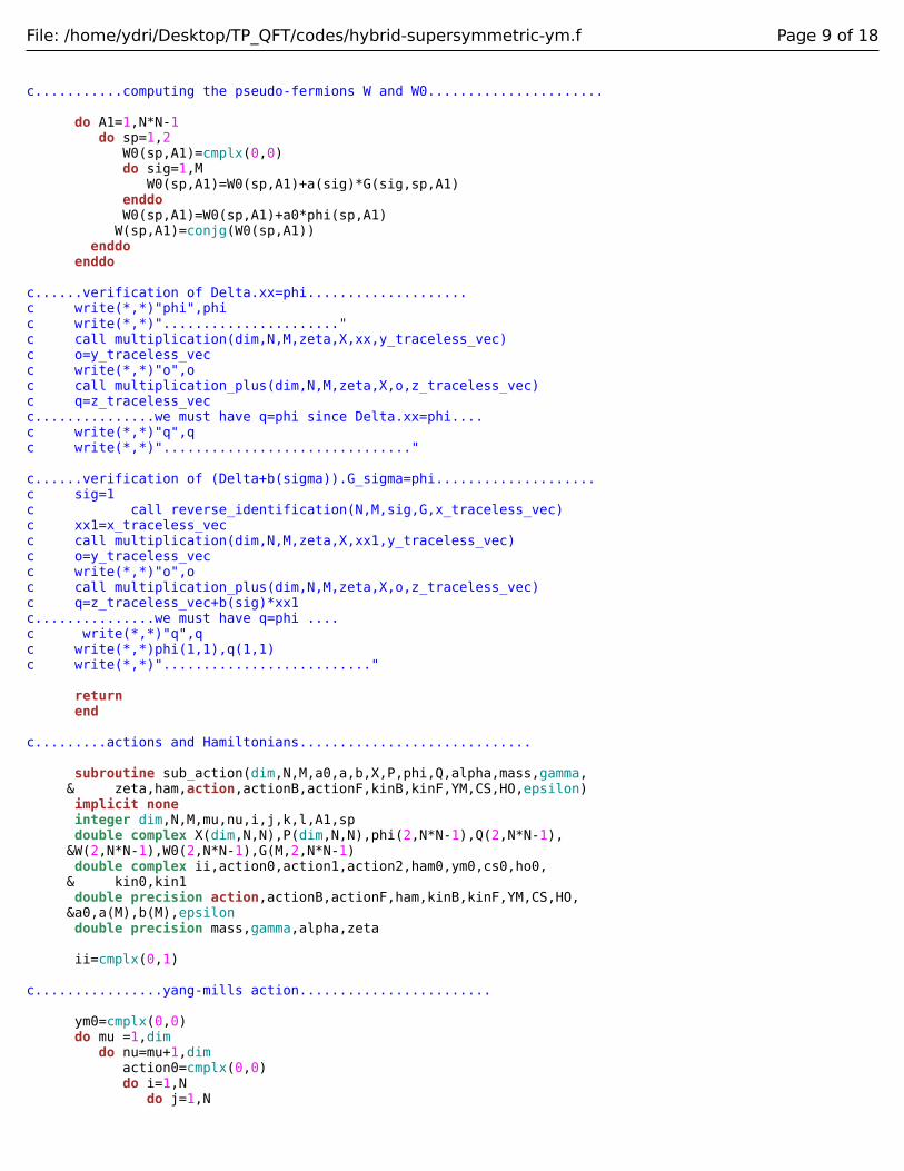
File: /home/ydri/Desktop/TP_QFT/codes/hybrid-supersymmetric-ym.f Page 9 of 18
c...........computing the pseudo-fermions W and W0...................... do A1=1,N*N-1 do sp=1,2 W0(sp,A1)=cmplx(0,0) do sig=1,M W0(sp,A1)=W0(sp,A1)+a(sig)*G(sig,sp,A1) enddo W0(sp,A1)=W0(sp,A1)+a0*phi(sp,A1) W(sp,A1)=conjg(W0(sp,A1)) enddo enddo c......verification of Delta.xx=phi....................c write(*,*)"phi",phic write(*,*)"......................"c call multiplication(dim,N,M,zeta,X,xx,y_traceless_vec)c o=y_traceless_vecc write(*,*)"o",oc call multiplication_plus(dim,N,M,zeta,X,o,z_traceless_vec)c q=z_traceless_vecc...............we must have q=phi since Delta.xx=phi.... c write(*,*)"q",qc write(*,*)"..............................." c......verification of (Delta+b(sigma)).G_sigma=phi....................c sig=1c call reverse_identification(N,M,sig,G,x_traceless_vec)c xx1=x_traceless_vecc call multiplication(dim,N,M,zeta,X,xx1,y_traceless_vec)c o=y_traceless_vecc write(*,*)"o",oc call multiplication_plus(dim,N,M,zeta,X,o,z_traceless_vec)c q=z_traceless_vec+b(sig)*xx1c...............we must have q=phi ....c write(*,*)"q",qc write(*,*)phi(1,1),q(1,1)c write(*,*)".........................." return end c.........actions and Hamiltonians............................. subroutine sub_action(dim,N,M,a0,a,b,X,P,phi,Q,alpha,mass,gamma, & zeta,ham,action,actionB,actionF,kinB,kinF,YM,CS,HO,epsilon) implicit none integer dim,N,M,mu,nu,i,j,k,l,A1,sp double complex X(dim,N,N),P(dim,N,N),phi(2,N*N-1),Q(2,N*N-1), &W(2,N*N-1),W0(2,N*N-1),G(M,2,N*N-1) double complex ii,action0,action1,action2,ham0,ym0,cs0,ho0, & kin0,kin1 double precision action,actionB,actionF,ham,kinB,kinF,YM,CS,HO, &a0,a(M),b(M),epsilon double precision mass,gamma,alpha,zeta ii=cmplx(0,1) c................yang-mills action........................ ym0=cmplx(0,0) do mu =1,dim do nu=mu+1,dim action0=cmplx(0,0) do i=1,N do j=1,N
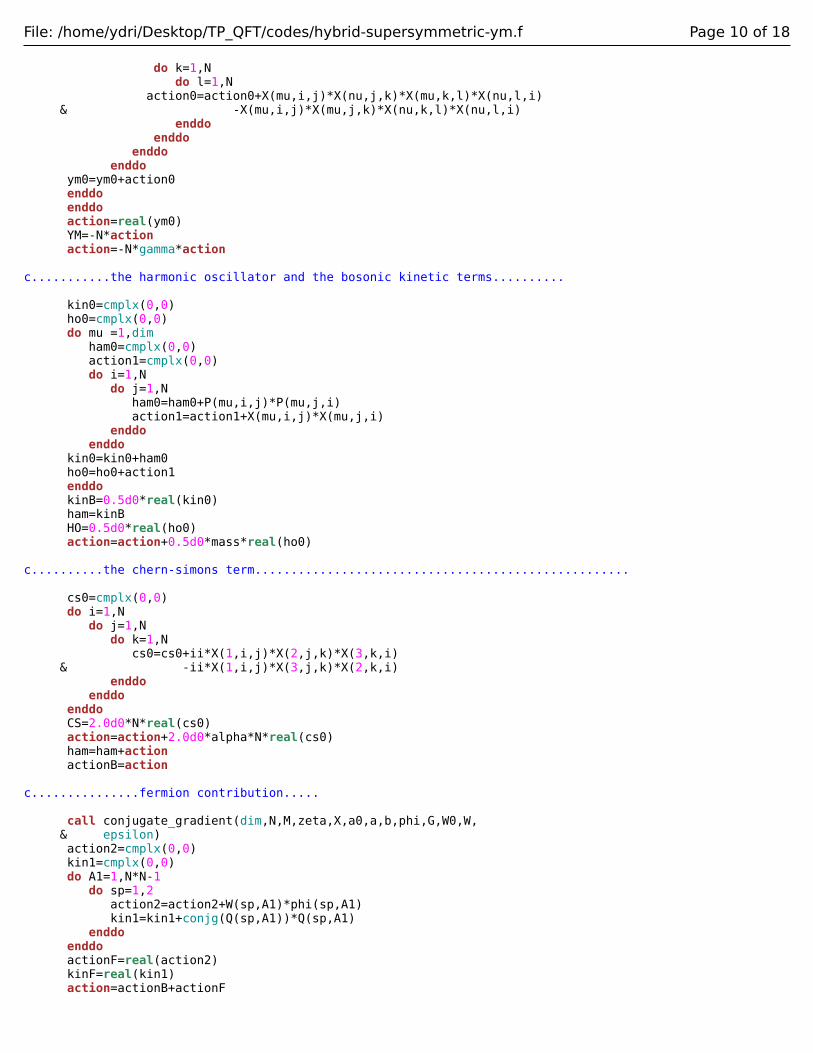
File: /home/ydri/Desktop/TP_QFT/codes/hybrid-supersymmetric-ym.f Page 10 of 18
do k=1,N do l=1,N action0=action0+X(mu,i,j)*X(nu,j,k)*X(mu,k,l)*X(nu,l,i) & -X(mu,i,j)*X(mu,j,k)*X(nu,k,l)*X(nu,l,i) enddo enddo enddo enddo ym0=ym0+action0 enddo enddo action=real(ym0) YM=-N*action action=-N*gamma*action c...........the harmonic oscillator and the bosonic kinetic terms.......... kin0=cmplx(0,0) ho0=cmplx(0,0) do mu =1,dim ham0=cmplx(0,0) action1=cmplx(0,0) do i=1,N do j=1,N ham0=ham0+P(mu,i,j)*P(mu,j,i) action1=action1+X(mu,i,j)*X(mu,j,i) enddo enddo kin0=kin0+ham0 ho0=ho0+action1 enddo kinB=0.5d0*real(kin0) ham=kinB HO=0.5d0*real(ho0) action=action+0.5d0*mass*real(ho0) c..........the chern-simons term.................................................... cs0=cmplx(0,0) do i=1,N do j=1,N do k=1,N cs0=cs0+ii*X(1,i,j)*X(2,j,k)*X(3,k,i) & -ii*X(1,i,j)*X(3,j,k)*X(2,k,i) enddo enddo enddo CS=2.0d0*N*real(cs0) action=action+2.0d0*alpha*N*real(cs0) ham=ham+action actionB=action
c...............fermion contribution..... call conjugate_gradient(dim,N,M,zeta,X,a0,a,b,phi,G,W0,W, & epsilon) action2=cmplx(0,0) kin1=cmplx(0,0) do A1=1,N*N-1 do sp=1,2 action2=action2+W(sp,A1)*phi(sp,A1) kin1=kin1+conjg(Q(sp,A1))*Q(sp,A1) enddo enddo actionF=real(action2) kinF=real(kin1) action=actionB+actionF
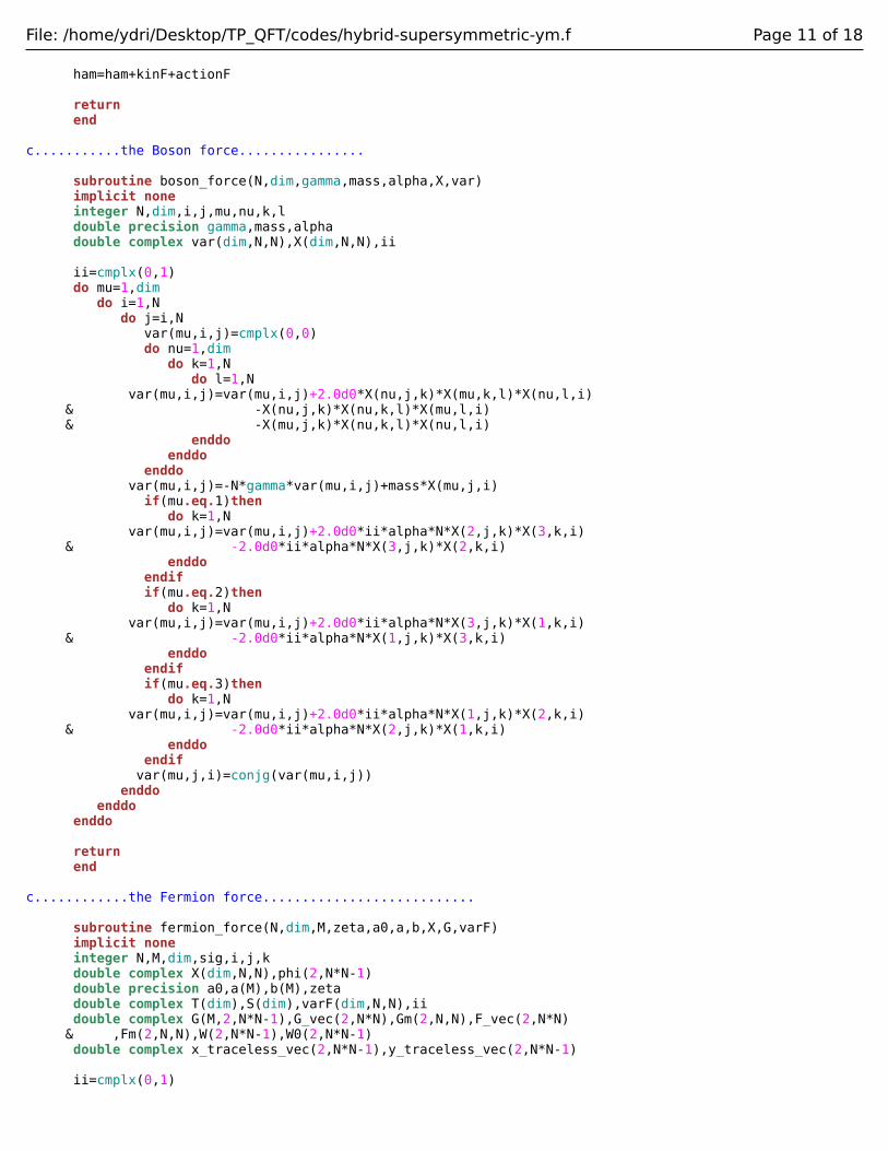
File: /home/ydri/Desktop/TP_QFT/codes/hybrid-supersymmetric-ym.f Page 11 of 18
ham=ham+kinF+actionF return end c...........the Boson force................
subroutine boson_force(N,dim,gamma,mass,alpha,X,var) implicit none integer N,dim,i,j,mu,nu,k,l double precision gamma,mass,alpha double complex var(dim,N,N),X(dim,N,N),ii ii=cmplx(0,1) do mu=1,dim do i=1,N do j=i,N var(mu,i,j)=cmplx(0,0) do nu=1,dim do k=1,N do l=1,N var(mu,i,j)=var(mu,i,j)+2.0d0*X(nu,j,k)*X(mu,k,l)*X(nu,l,i) & -X(nu,j,k)*X(nu,k,l)*X(mu,l,i) & -X(mu,j,k)*X(nu,k,l)*X(nu,l,i) enddo enddo enddo var(mu,i,j)=-N*gamma*var(mu,i,j)+mass*X(mu,j,i) if(mu.eq.1)then do k=1,N var(mu,i,j)=var(mu,i,j)+2.0d0*ii*alpha*N*X(2,j,k)*X(3,k,i) & -2.0d0*ii*alpha*N*X(3,j,k)*X(2,k,i) enddo endif if(mu.eq.2)then do k=1,N var(mu,i,j)=var(mu,i,j)+2.0d0*ii*alpha*N*X(3,j,k)*X(1,k,i) & -2.0d0*ii*alpha*N*X(1,j,k)*X(3,k,i) enddo endif if(mu.eq.3)then do k=1,N var(mu,i,j)=var(mu,i,j)+2.0d0*ii*alpha*N*X(1,j,k)*X(2,k,i) & -2.0d0*ii*alpha*N*X(2,j,k)*X(1,k,i) enddo endif var(mu,j,i)=conjg(var(mu,i,j)) enddo enddo enddo return end
c............the Fermion force........................... subroutine fermion_force(N,dim,M,zeta,a0,a,b,X,G,varF) implicit none integer N,M,dim,sig,i,j,k double complex X(dim,N,N),phi(2,N*N-1) double precision a0,a(M),b(M),zeta double complex T(dim),S(dim),varF(dim,N,N),ii double complex G(M,2,N*N-1),G_vec(2,N*N),Gm(2,N,N),F_vec(2,N*N) & ,Fm(2,N,N),W(2,N*N-1),W0(2,N*N-1) double complex x_traceless_vec(2,N*N-1),y_traceless_vec(2,N*N-1) ii=cmplx(0,1)
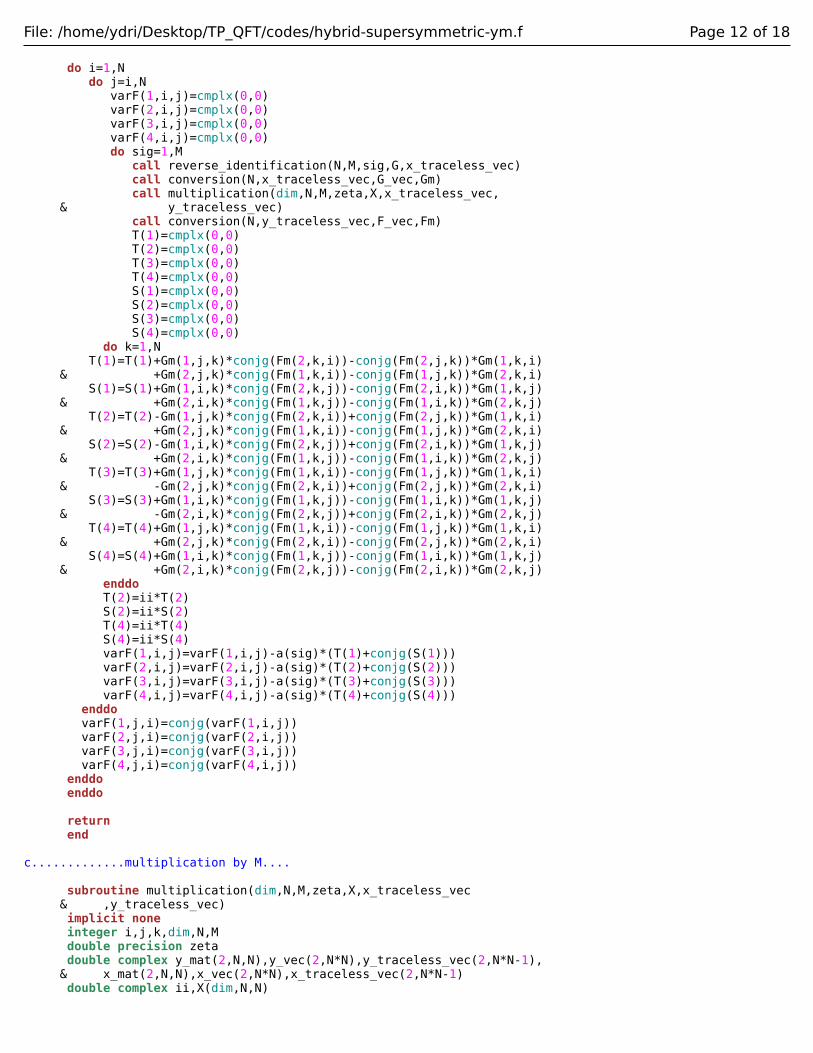
File: /home/ydri/Desktop/TP_QFT/codes/hybrid-supersymmetric-ym.f Page 12 of 18
do i=1,N do j=i,N varF(1,i,j)=cmplx(0,0) varF(2,i,j)=cmplx(0,0) varF(3,i,j)=cmplx(0,0) varF(4,i,j)=cmplx(0,0) do sig=1,M call reverse_identification(N,M,sig,G,x_traceless_vec) call conversion(N,x_traceless_vec,G_vec,Gm) call multiplication(dim,N,M,zeta,X,x_traceless_vec, & y_traceless_vec) call conversion(N,y_traceless_vec,F_vec,Fm) T(1)=cmplx(0,0) T(2)=cmplx(0,0) T(3)=cmplx(0,0) T(4)=cmplx(0,0) S(1)=cmplx(0,0) S(2)=cmplx(0,0) S(3)=cmplx(0,0) S(4)=cmplx(0,0) do k=1,N T(1)=T(1)+Gm(1,j,k)*conjg(Fm(2,k,i))-conjg(Fm(2,j,k))*Gm(1,k,i) & +Gm(2,j,k)*conjg(Fm(1,k,i))-conjg(Fm(1,j,k))*Gm(2,k,i) S(1)=S(1)+Gm(1,i,k)*conjg(Fm(2,k,j))-conjg(Fm(2,i,k))*Gm(1,k,j) & +Gm(2,i,k)*conjg(Fm(1,k,j))-conjg(Fm(1,i,k))*Gm(2,k,j) T(2)=T(2)-Gm(1,j,k)*conjg(Fm(2,k,i))+conjg(Fm(2,j,k))*Gm(1,k,i) & +Gm(2,j,k)*conjg(Fm(1,k,i))-conjg(Fm(1,j,k))*Gm(2,k,i) S(2)=S(2)-Gm(1,i,k)*conjg(Fm(2,k,j))+conjg(Fm(2,i,k))*Gm(1,k,j) & +Gm(2,i,k)*conjg(Fm(1,k,j))-conjg(Fm(1,i,k))*Gm(2,k,j) T(3)=T(3)+Gm(1,j,k)*conjg(Fm(1,k,i))-conjg(Fm(1,j,k))*Gm(1,k,i) & -Gm(2,j,k)*conjg(Fm(2,k,i))+conjg(Fm(2,j,k))*Gm(2,k,i) S(3)=S(3)+Gm(1,i,k)*conjg(Fm(1,k,j))-conjg(Fm(1,i,k))*Gm(1,k,j) & -Gm(2,i,k)*conjg(Fm(2,k,j))+conjg(Fm(2,i,k))*Gm(2,k,j) T(4)=T(4)+Gm(1,j,k)*conjg(Fm(1,k,i))-conjg(Fm(1,j,k))*Gm(1,k,i) & +Gm(2,j,k)*conjg(Fm(2,k,i))-conjg(Fm(2,j,k))*Gm(2,k,i) S(4)=S(4)+Gm(1,i,k)*conjg(Fm(1,k,j))-conjg(Fm(1,i,k))*Gm(1,k,j) & +Gm(2,i,k)*conjg(Fm(2,k,j))-conjg(Fm(2,i,k))*Gm(2,k,j) enddo T(2)=ii*T(2) S(2)=ii*S(2) T(4)=ii*T(4) S(4)=ii*S(4) varF(1,i,j)=varF(1,i,j)-a(sig)*(T(1)+conjg(S(1))) varF(2,i,j)=varF(2,i,j)-a(sig)*(T(2)+conjg(S(2))) varF(3,i,j)=varF(3,i,j)-a(sig)*(T(3)+conjg(S(3))) varF(4,i,j)=varF(4,i,j)-a(sig)*(T(4)+conjg(S(4))) enddo varF(1,j,i)=conjg(varF(1,i,j)) varF(2,j,i)=conjg(varF(2,i,j)) varF(3,j,i)=conjg(varF(3,i,j)) varF(4,j,i)=conjg(varF(4,i,j)) enddo enddo return end c.............multiplication by M....
subroutine multiplication(dim,N,M,zeta,X,x_traceless_vec & ,y_traceless_vec) implicit none integer i,j,k,dim,N,M double precision zeta double complex y_mat(2,N,N),y_vec(2,N*N),y_traceless_vec(2,N*N-1), & x_mat(2,N,N),x_vec(2,N*N),x_traceless_vec(2,N*N-1) double complex ii,X(dim,N,N)

File: /home/ydri/Desktop/TP_QFT/codes/hybrid-supersymmetric-ym.f Page 13 of 18
ii=cmplx(0,1) call conversion(N,x_traceless_vec,x_vec,x_mat) do j=1,N do i=1,N y_mat(1,j,i)=zeta*x_mat(1,i,j) y_mat(2,j,i)=zeta*x_mat(2,i,j) do k=1,N y_mat(1,j,i)=y_mat(1,j,i) & +X(3,i,k)*x_mat(1,k,j)-x_mat(1,i,k)*X(3,k,j) & +ii*X(4,i,k)*x_mat(1,k,j)-ii*x_mat(1,i,k)*X(4,k,j) & +X(1,i,k)*x_mat(2,k,j)-x_mat(2,i,k)*X(1,k,j) & -ii*X(2,i,k)*x_mat(2,k,j)+ii*x_mat(2,i,k)*X(2,k,j) y_mat(2,j,i)=y_mat(2,j,i) & -X(3,i,k)*x_mat(2,k,j)+x_mat(2,i,k)*X(3,k,j) & +ii*X(4,i,k)*x_mat(2,k,j)-ii*x_mat(2,i,k)*X(4,k,j) & +X(1,i,k)*x_mat(1,k,j)-x_mat(1,i,k)*X(1,k,j) & +ii*X(2,i,k)*x_mat(1,k,j)-ii*x_mat(1,i,k)*X(2,k,j) enddo enddo enddo call reverse_conversion(N,y_mat,y_vec,y_traceless_vec) return end c.............multiplication by M^+....
subroutine multiplication_plus(dim,N,M,zeta,X,y_traceless_vec & ,z_traceless_vec) implicit none integer i,j,k,dim,N,M double precision zeta double complex z_mat(2,N,N),z_vec(2,N*N),z_traceless_vec(2,N*N-1), & y_mat(2,N,N),y_vec(2,N*N),y_traceless_vec(2,N*N-1) double complex ii,X(dim,N,N) ii=cmplx(0,1) call conversion(N,y_traceless_vec,y_vec,y_mat) do j=1,N do i=1,N z_mat(1,j,i)=zeta*y_mat(1,i,j) z_mat(2,j,i)=zeta*y_mat(2,i,j)
do k=1,N z_mat(1,j,i)=z_mat(1,j,i) & -X(3,k,i)*y_mat(1,k,j)+y_mat(1,i,k)*X(3,j,k) & +ii*X(4,k,i)*y_mat(1,k,j)-ii*y_mat(1,i,k)*X(4,j,k) & -X(1,k,i)*y_mat(2,k,j)+y_mat(2,i,k)*X(1,j,k) & +ii*X(2,k,i)*y_mat(2,k,j)-ii*y_mat(2,i,k)*X(2,j,k) z_mat(2,j,i)=z_mat(2,j,i) & +X(3,k,i)*y_mat(2,k,j)-y_mat(2,i,k)*X(3,j,k) & +ii*X(4,k,i)*y_mat(2,k,j)-ii*y_mat(2,i,k)*X(4,j,k) & -X(1,k,i)*y_mat(1,k,j)+y_mat(1,i,k)*X(1,j,k) & -ii*X(2,k,i)*y_mat(1,k,j)+ii*y_mat(1,i,k)*X(2,j,k) enddo enddo enddo call reverse_conversion(N,z_mat,z_vec,z_traceless_vec) return end c.... given x_traceless_vec we construct x_vec and x_mat........ subroutine conversion(N,x_traceless_vec,x_vec,x_mat) implicit none integer N,i,j,A1,sp

File: /home/ydri/Desktop/TP_QFT/codes/hybrid-supersymmetric-ym.f Page 14 of 18
double complex x_traceless_vec(2,N*N-1),x_vec(2,N*N),x_mat(2,N,N) & ,xx do sp=1,2 xx=0.0d0 do i=1,N do j=1,N A1=N*(i-1)+j if (A1.lt.N*N) then x_vec(sp,A1)=x_traceless_vec(sp,A1) if (i.eq.j) then xx=xx-x_traceless_vec(sp,A1) endif endif x_mat(sp,i,j)=x_vec(sp,A1) enddo enddo x_vec(sp,N*N)=xx x_mat(sp,N,N)=x_vec(sp,N*N) enddo return end c......given x_mat we construct x_vec and x_traceless_vec... subroutine reverse_conversion(N,x_mat,x_vec,x_traceless_vec) implicit none integer N,i,j,A1,sp double complex x_mat(2,N,N),x_vec(2,N*N),x_traceless_vec(2,N*N-1) do sp=1,2 x_vec(sp,N*N)=x_mat(sp,N,N) do i=1,N do j=1,N A1=N*(i-1)+j if (A1.lt.N*N) then x_vec(sp,A1)=x_mat(sp,i,j) if (i.eq.j)then x_traceless_vec(sp,A1)=x_vec(sp,A1)-x_vec(sp,N*N) else x_traceless_vec(sp,A1)=x_vec(sp,A1) endif
endif enddo enddo enddo return end c...............generation of Gaussian noise for the field P............ subroutine gaussian(idum,dim,N,P) implicit none integer dim,N,mu,i,j,idum double precision pi,phi,r,ran2 double complex ii,P(dim,N,N) pi=dacos(-1.0d0) ii=cmplx(0,1) do mu=1,dimc.............diagonal......... do i=1,N phi=2.0d0*pi*ran2(idum) r=dsqrt(-2.0d0*dlog(1.0d0-ran2(idum))) P(mu,i,i)=r*dcos(phi)

File: /home/ydri/Desktop/TP_QFT/codes/hybrid-supersymmetric-ym.f Page 15 of 18
enddoc.......off diagonal............ do i=1,N do j=i+1,N phi=2.0d0*pi*ran2(idum) r=dsqrt(-1.0d0*dlog(1.0d0-ran2(idum))) P(mu,i,j)=r*dcos(phi)+ii*r*dsin(phi) P(mu,j,i)=conjg(P(mu,i,j)) enddo enddo enddo return end
c...............generation of Gaussian noise for the field Q............ subroutine gaussian_plus(idum,N,Q) implicit none integer N,A1,sp,idum double precision pi,phi,r,ran2 double complex Q(2,N*N-1),ii pi=dacos(-1.0d0) ii=cmplx(0,1) do A1=1,N*N-1 do sp=1,2 phi=2.0d0*pi*ran2(idum) r=dsqrt(-1.0d0*dlog(1.0d0-ran2(idum))) Q(sp,A1)=r*dcos(phi)+ii*r*dsin(phi) enddo enddo return end
c.........hot start................. subroutine hot(N,dim,idum,inn,X) integer mu,i,j,N,dim,idum double complex X(dim,N,N) double precision xx,y,inn,ran2
do mu=1,dim do i=1,N do j=i,N if (j.ne.i) then xx=(2.0d0*ran2(idum)-1.0d0)*inn y=(2.0d0*ran2(idum)-1.0d0)*inn X(mu,i,j)=cmplx(xx,y) X(mu,j,i)=cmplx(xx,-y) else xx=(2.0d0*ran2(idum)-1.0d0)*inn X(mu,i,j)=xx endif enddo enddo enddo
return end c...........cold start...................... subroutine cold(N,dim,idum,X) integer mu,i,j,N,dim,idum double complex X(dim,N,N)
File: /home/ydri/Desktop/TP_QFT/codes/hybrid-supersymmetric-ym.f Page 16 of 18
do mu=1,dim do i=1,N do j=1,N X(mu,i,j)=cmplx(0,0) enddo enddo enddo return end c..........the jackknife estimator...............
subroutine jackknife_binning(TMC,f,average,error) integer i,j,TMC,zbin,nbin double precision xm double precision f(1:TMC),sumf,y(1:TMC) double precision sig0,sig,error,average sig0=0.0d0 sumf=0.0d0 do i=1,TMC sumf=sumf+f(i) enddo xm=sumf/TMC zbin=1 nbin=int(TMC/zbin) sig=0.0d0 do i=1,nbin,1 y(i)=sumf do j=1,zbin y(i)=y(i)-f((i-1)*zbin+j ) enddo y(i)= y(i)/(TMC-zbin) sig=sig+((nbin-1.0d0)/nbin)*(y(i)-xm)*(y(i)-xm) enddo sig=dsqrt(sig) if (sig0 .lt. sig) sig0=sig error=sig0 average=xm return
end c.............the random number generator ran2.............
function ran2(idum) implicit none integer idum,IM1,IM2,IMM1,IA1,IA2,IQ1,IQ2,IR1,IR2,NTAB,NDIV real AM,EPS,RNMX double precision ran2 parameter (IM1=2147483563,IM2=2147483399,AM=1./IM1,IMM1=IM1-1, & IA1=40014,IA2=40692,IQ1=53668,IQ2=52774,IR1=12211, & IR2=3791,NTAB=32,NDIV=1+IMM1/NTAB,EPS=1.2E-7,RNMX=1.-EPS) integer idum2,j,k,iv(NTAB),iy SAVE iv,iy,idum2 DATA idum2/123456789/,iv/NTAB*0/,iy/0/ if (idum.le.0) then idum=max(-idum,1) idum2=idum do j=NTAB+8,1,-1 k=idum/IQ1 idum=IA1*(idum-k*IQ1)-k*IR1 if (idum.lt.0) idum=idum+IM1 if (j.le.NTAB) iv(j)=idum

File: /home/ydri/Desktop/TP_QFT/codes/hybrid-supersymmetric-ym.f Page 17 of 18
enddo iy=iv(1) endif k=idum/IQ1 idum=IA1*(idum-k*IQ1)-k*IR1 if (idum.lt.0) idum=idum+IM1 k=idum2/IQ2 idum2=IA2*(idum2-k*IQ2)-k*IR2 if (idum2.lt.0) idum2=idum2+IM2 j=1+iy/NDIV iy=iv(j)-idum2 iv(j)=idum if (iy.lt.1) iy=iy+IMM1 ran2=min(AM*iy,RNMX)
return end
c...........defining an array from a vector....
subroutine identification(N,M,sig,x_traceless_vec,G) implicit none integer N,M,sig,sp,A1 double complex G(M,2,N*N-1),x_traceless_vec(2,N*N-1) do sp=1,2 do A1=1,N*N-1 G(sig,sp,A1)=x_traceless_vec(sp,A1) enddo enddo
return end c.......defining a vector from an array.......
subroutine reverse_identification(N,M,sig,G,x_traceless_vec) implicit none integer N,M,sig,sp,A1 double complex G(M,2,N*N-1),x_traceless_vec(2,N*N-1)
do sp=1,2 do A1=1,N*N-1 x_traceless_vec(sp,A1)=G(sig,sp,A1) enddo enddo return end c.........adjusting interval..................
subroutine adjust_inn(cou,pa,dt,time,Rejec,Accept, & nn,target_pa_high,target_pa_low,dt_max,dt_min,inc,dec) implicit none double precision dt,pa,Rejec,Accept integer time,cou,cou1 integer nn double precision target_pa_high,target_pa_low,dt_max,dt_min,inc, & dec,rho1,rho2,dtnew c.....pa acceptance rate............ pa=(Accept)/(Rejec+Accept) cou1=mod(cou,nn) if (cou1.eq.0)thenc........fixing the acceptance rate between 90 % 70 %.................. if (pa.ge.target_pa_high) then

File: /home/ydri/Desktop/TP_QFT/codes/hybrid-supersymmetric-ym.f Page 18 of 18
dtnew=dt*inc if (dtnew.le.dt_max)then dt=dtnew else dt=dt_max endif endif if (pa.le.target_pa_low) then dtnew=dt*dec if (dtnew.ge.dt_min)then dt=dtnew else dt=dt_min endif endif endif return end

File: /home/ydri/Desktop/TP_QFT/codes/u-one-on-the-lattice.f Page 1 of 11
program my_u_one_on_the_lattice implicit none integer dim,N,NT,i,j,k,l,mu,idum,tther,tmont,nther,nmont,counter,T integer tcor,ncor,betai,p,q double precision accept,reject,flip parameter (dim=4,N=4,NT=4,nther=2**(14),nmont=2**(14),ncor=2**4) parameter (T=100*(nther+nmont*ncor)) double precision beta,ran2,variation,epsilon & ,epsilon0,pi,acceptance,avera,erro,tau,deltau double complex U(dim,N,N,N,NT),ii,X,XX(0:T) double precision W11,W22,W33,W12,W13,W23,W21,W31,W32 double precision acti(1:nmont),acti_mean,acti_error, & action double precision acti_pp(1:nmont),acti_pp_mean,acti_pp_error, & action_pp double precision cv(1:nmont),cv_mean,cv_error double precision plaq1(1:nmont),plaq1_mean,plaq1_error double precision plaq2(1:nmont),plaq2_mean,plaq2_error double precision plaq3(1:nmont),plaq3_mean,plaq3_error double precision plaq4(1:nmont),plaq4_mean,plaq4_error double precision plaq5(1:nmont),plaq5_mean,plaq5_error double precision plaq6(1:nmont),plaq6_mean,plaq6_error double precision plaq7(1:nmont),plaq7_mean,plaq7_error double precision plaq8(1:nmont),plaq8_mean,plaq8_error double precision plaq9(1:nmont),plaq9_mean,plaq9_error double precision tension1,error_tension1,tension2,error_tension2, & tension3,error_tension3,tension4,error_tension4 c.........initialization of the random number generator.....................
idum=-148175 call seed(idum)
c..........initialization of other parameters...............................
counter=0 accept=0 reject=0 flip=0 ii=cmplx(0,1) pi=dacos(-1.0d0) epsilon=pi c.................gauge coupling constant..................
do betai=1,1 beta=1.9d0-betai*0.1 c.............initialization of the link variables................ do mu=1,dim do i=1,N do j=1,N do k=1,N do l=1,NTc.........ordered start for coulomb phase while disordered start for confinment phase.. if(beta.ge.1.0d0)then epsilon0=0.0d0 else epsilon0=2.0d0*ran2(idum)-1.0d0 epsilon0=epsilon*epsilon0 endif U(mu,i,j,k,l)=dcos(epsilon0)+ii*dsin(epsilon0) enddo enddo enddo enddo

File: /home/ydri/Desktop/TP_QFT/codes/u-one-on-the-lattice.f Page 2 of 11
enddo c................thermalization............. do tther=1,nther call metropolis(U,beta,dim,N,NT,accept,reject,flip,acceptance, & epsilon,counter,XX,T) enddo
c..............monte carlo evolution................................... do tmont=1,nmont do tcor=1,ncor call metropolis(U,beta,dim,N,NT,accept,reject,flip,acceptance, & epsilon,counter,XX,T) enddo call actio(U,dim,N,NT,beta,action,action_pp) acti(tmont)=action acti_pp(tmont)=action_pp plaq1(tmont)=0.0d0 plaq2(tmont)=0.0d0 plaq3(tmont)=0.0d0 plaq4(tmont)=0.0d0 plaq5(tmont)=0.0d0 plaq6(tmont)=0.0d0 plaq7(tmont)=0.0d0 plaq8(tmont)=0.0d0 plaq9(tmont)=0.0d0 do i=1,N do j=1,N do k=1,N do l=1,NT p=1 q=4 call Wilson_Loop(U,dim,N,NT,i,j,k,l,p,q, & W11,W22,W33,W12,W13,W23,W21,W31,W32) plaq1(tmont)=plaq1(tmont)+W11 plaq2(tmont)=plaq2(tmont)+W22 plaq3(tmont)=plaq3(tmont)+W33 plaq4(tmont)=plaq4(tmont)+W12 plaq5(tmont)=plaq5(tmont)+W13 plaq6(tmont)=plaq6(tmont)+W23 plaq7(tmont)=plaq7(tmont)+W21 plaq8(tmont)=plaq8(tmont)+W31 plaq9(tmont)=plaq9(tmont)+W32 enddo enddo enddo enddo plaq1(tmont)=plaq1(tmont)/(N**3*NT) plaq2(tmont)=plaq2(tmont)/(N**3*NT) plaq3(tmont)=plaq3(tmont)/(N**3*NT) plaq4(tmont)=plaq4(tmont)/(N**3*NT) plaq5(tmont)=plaq5(tmont)/(N**3*NT) plaq6(tmont)=plaq6(tmont)/(N**3*NT) plaq7(tmont)=plaq7(tmont)/(N**3*NT) plaq8(tmont)=plaq8(tmont)/(N**3*NT) plaq9(tmont)=plaq9(tmont)/(N**3*NT) enddo
c......................measurements........................
c......................action............... call jackknife_binning(nmont,acti,acti_mean,acti_error) write(11,*)beta,acti_mean,acti_errorc write(*,*)beta,acti_mean,acti_error

File: /home/ydri/Desktop/TP_QFT/codes/u-one-on-the-lattice.f Page 3 of 11
c..................action per plaquette.......... call jackknife_binning(nmont,acti_pp,acti_pp_mean,acti_pp_error) write(12,*)beta,acti_pp_mean,acti_pp_errorc write(*,*)beta,acti_pp_mean,acti_pp_error
c.......................specific heat............. do tmont=1,nmont cv(tmont)=(acti(tmont)-acti_mean)**2 enddo call jackknife_binning(nmont,cv,cv_mean,cv_error) write(13,*)beta,cv_mean,cv_errorc write(*,*)beta,cv_mean,cv_error
c................Wilson loops................ call jackknife_binning(nmont,plaq1,plaq1_mean,plaq1_error) write(15,*)beta,plaq1_mean,plaq1_errorc write(*,*)beta,plaq1_mean,plaq1_error call jackknife_binning(nmont,plaq2,plaq2_mean,plaq2_error) write(16,*)beta,plaq2_mean,plaq2_errorc write(*,*)beta,plaq2_mean,plaq2_error call jackknife_binning(nmont,plaq3,plaq3_mean,plaq3_error) write(17,*)beta,plaq3_mean,plaq3_errorc write(*,*)beta,plaq3_mean,plaq3_error call jackknife_binning(nmont,plaq4,plaq4_mean,plaq4_error) write(18,*)beta,plaq4_mean,plaq4_errorc write(*,*)beta,plaq4_mean,plaq4_error call jackknife_binning(nmont,plaq5,plaq5_mean,plaq5_error) write(19,*)beta,plaq5_mean,plaq5_errorc write(*,*)beta,plaq5_mean,plaq5_error call jackknife_binning(nmont,plaq6,plaq6_mean,plaq6_error) write(20,*)beta,plaq6_mean,plaq6_errorc write(*,*)beta,plaq6_mean,plaq6_error call jackknife_binning(nmont,plaq7,plaq7_mean,plaq7_error) write(23,*)beta,plaq7_mean,plaq7_errorc write(*,*)beta,plaq7_mean,plaq7_error call jackknife_binning(nmont,plaq8,plaq8_mean,plaq8_error) write(24,*)beta,plaq8_mean,plaq8_errorc write(*,*)beta,plaq8_mean,plaq8_error call jackknife_binning(nmont,plaq9,plaq9_mean,plaq9_error) write(25,*)beta,plaq9_mean,plaq9_errorc write(*,*)beta,plaq9_mean,plaq9_error c..............Creutz ratios:string tension.............c...........chi22.......... tension1=(plaq2_mean*plaq1_mean)/(plaq4_mean*plaq7_mean)c..........chi33..... tension2=(plaq3_mean*plaq2_mean)/(plaq6_mean*plaq9_mean)c..........chi23...... tension3=(plaq6_mean*plaq4_mean)/(plaq2_mean*plaq5_mean)c.........chi32.......... tension4=(plaq9_mean*plaq7_mean)/(plaq2_mean*plaq8_mean) tension1=dabs(tension1) tension2=dabs(tension2) tension3=dabs(tension3) tension4=dabs(tension4) tension1=-dlog(tension1) tension2=-dlog(tension2) tension3=-dlog(tension3) tension4=-dlog(tension4) error_tension1=plaq2_error/plaq2_mean+plaq1_error/plaq1_mean & -plaq4_error/plaq4_mean-plaq7_error/plaq7_mean error_tension1=dabs(error_tension1) error_tension2=plaq3_error/plaq3_mean+plaq2_error/plaq2_mean & -plaq6_error/plaq6_mean -plaq9_error/plaq9_mean error_tension2=dabs(error_tension2) error_tension3=plaq6_error/plaq6_mean+plaq4_error/plaq4_mean

File: /home/ydri/Desktop/TP_QFT/codes/u-one-on-the-lattice.f Page 4 of 11
& -plaq2_error/plaq2_mean -plaq5_error/plaq5_mean error_tension3=dabs(error_tension3) error_tension4=plaq9_error/plaq9_mean+plaq7_error/plaq7_mean & -plaq2_error/plaq2_mean -plaq8_error/plaq8_mean error_tension4=dabs(error_tension4)
write(22,*)beta,tension1,error_tension1,tension2,error_tension2, & tension3,error_tension3,tension4,error_tension4c write(*,*)beta,tension1,error_tension1,tension2,error_tension2,c & tension3,error_tension3,tension4,error_tension4 enddo return end
c...............metropolis algorithm................. subroutine metropolis(U,beta,dim,N,NT,accept,reject,flip, & acceptance,epsilon,counter,XX,T) implicit none integer dim,N,NT,nu,mu,i,j,k,l,idum,counter,counter0,nn,T double precision accept,reject,flip,nn0 double precision epsilon,epsilon0,beta,variation,proba,r,ran2,pi, & modulus,acceptance double complex U(dim,N,N,N,NT),X,ii,XX(0:T) pi=dacos(-1.0d0) ii=cmplx(0,1) epsilon0=2.0d0*ran2(idum)-1.0d0 epsilon0=epsilon*epsilon0 XX(counter)=dcos(epsilon0)+ii*dsin(epsilon0) XX(counter+1)=dcos(epsilon0)-ii*dsin(epsilon0) counter0=counter+1 counter=counter+2 do mu=1,dim do i=1,N do j=1,N do k=1,N do l=1,NT nn0=counter0*ran2(idum) nn=nint(nn0) X=XX(nn) call variatio(U,X,beta,dim,N,NT,mu,i,j,k,l,variation) if(variation.gt.0)then proba=dexp(-variation) r=ran2(idum) if(proba.gt.r)then U(mu,i,j,k,l)=X*U(mu,i,j,k,l) accept=accept+1 else reject=reject+1 endif else U(mu,i,j,k,l)=X*U(mu,i,j,k,l) flip=flip+1 endif modulus=U(mu,i,j,k,l)*conjg(U(mu,i,j,k,l)) modulus=dsqrt(modulus) U(mu,i,j,k,l)=U(mu,i,j,k,l)/modulus enddo enddo enddo enddo enddo
File: /home/ydri/Desktop/TP_QFT/codes/u-one-on-the-lattice.f Page 5 of 11
c.......for the range of N and NT considered the acceptance rate is already sufficiently high so we can simply disable the adjust subroutine....we observed that the acceptance rate decreases as we increase N and NT...... call adjust(epsilon,flip,accept,reject,acceptance) c write(*,*)flip,accept,reject,acceptance
return end c...........adjusting...........................
subroutine adjust(epsilon,flip,accept,reject,acceptance) implicit none double precision epsilon,acceptance double precision flip,accept,reject,ran2 integer idum acceptance=(flip+accept)/(flip+accept+reject) if (acceptance.ge.0.5d0) then epsilon=epsilon*1.2d0 endif if(acceptance.le.0.45d0) then epsilon=epsilon*0.8d0 endif return end
c........................variation..................... subroutine variatio(U,X,beta,dim,N,NT,mu,i,j,k,l,variation) implicit none integer dim,N,NT,nu,mu,i,j,k,l,idum double precision epsilon,epsilon0,beta,variation,ran2,pi double complex U(dim,N,N,N,NT),staple,ii,X call stapl(U,dim,N,NT,mu,i,j,k,l,staple) variation=-0.5d0*beta*((X-1.0d0)*U(mu,i,j,k,l)*staple & + conjg((X-1.0d0)*U(mu,i,j,k,l)*staple)) return end
c.................staple.................................... subroutine stapl(U,dim,N,NT,mu,i,j,k,l,staple) implicit none integer dim,N,NT,nu,mu,i,j,k,l,i0,ip(N),im(N),ipT(NT),imT(NT), & ipn(1:N,1:N),ipnT(1:N,1:N) double precision beta double complex U(dim,N,N,N,NT),staple call index_array(N,NT,ip,im,ipT,imT,ipn,ipnT) if(mu.eq.1)then staple=U(2,ip(i),j,k,l)*conjg(U(mu,i,ip(j),k,l))* & conjg(U(2,i,j,k,l)) & +conjg(U(2,ip(i),im(j),k,l))*conjg(U(mu,i,im(j),k,l)) & *U(2,i,im(j),k,l) & +U(3,ip(i),j,k,l)*conjg(U(mu,i,j,ip(k),l))*conjg(U(3,i,j,k,l)) & +conjg(U(3,ip(i),j,im(k),l))*conjg(U(mu,i,j,im(k),l)) & *U(3,i,j,im(k),l) & +U(4,ip(i),j,k,l)*conjg(U(mu,i,j,k,ipT(l)))*conjg(U(4,i,j,k,l)) & +conjg(U(4,ip(i),j,k,imT(l)))*conjg(U(mu,i,j,k,imT(l))) & *U(4,i,j,k,imT(l)) endif
File: /home/ydri/Desktop/TP_QFT/codes/u-one-on-the-lattice.f Page 6 of 11
if(mu.eq.2)then staple=U(1,i,ip(j),k,l)*conjg(U(mu,ip(i),j,k,l))* & conjg(U(1,i,j,k,l)) & +conjg(U(1,im(i),ip(j),k,l))*conjg(U(mu,im(i),j,k,l)) & *U(1,im(i),j,k,l) & +U(3,i,ip(j),k,l)*conjg(U(mu,i,j,ip(k),l))*conjg(U(3,i,j,k,l)) & +conjg(U(3,i,ip(j),im(k),l))*conjg(U(mu,i,j,im(k),l)) & *U(3,i,j,im(k),l) & +U(4,i,ip(j),k,l)*conjg(U(mu,i,j,k,ipT(l)))*conjg(U(4,i,j,k,l)) & +conjg(U(4,i,ip(j),k,imT(l)))*conjg(U(mu,i,j,k,imT(l))) & *U(4,i,j,k,imT(l)) endif if(mu.eq.3)then staple=U(1,i,j,ip(k),l)*conjg(U(mu,ip(i),j,k,l)) & *conjg(U(1,i,j,k,l)) & +conjg(U(1,im(i),j,ip(k),l))*conjg(U(mu,im(i),j,k,l)) & *U(1,im(i),j,k,l) & +U(2,i,j,ip(k),l)*conjg(U(mu,i,ip(j),k,l))*conjg(U(2,i,j,k,l)) & +conjg(U(2,i,im(j),ip(k),l))*conjg(U(mu,i,im(j),k,l)) & *U(2,i,im(j),k,l) & +U(4,i,j,ip(k),l)*conjg(U(mu,i,j,k,ipT(l)))*conjg(U(4,i,j,k,l)) & +conjg(U(4,i,j,ip(k),imT(l)))*conjg(U(mu,i,j,k,imT(l))) & *U(4,i,j,k,imT(l)) endif if(mu.eq.4)then staple=U(1,i,j,k,ipT(l))*conjg(U(mu,ip(i),j,k,l)) & *conjg(U(1,i,j,k,l)) & +conjg(U(1,im(i),j,k,ipT(l)))*conjg(U(mu,im(i),j,k,l)) & *U(1,im(i),j,k,l) & +U(2,i,j,k,ipT(l))*conjg(U(mu,i,ip(j),k,l))*conjg(U(2,i,j,k,l)) & +conjg(U(2,i,im(j),k,ipT(l)))*conjg(U(mu,i,im(j),k,l)) & *U(2,i,im(j),k,l) & +U(3,i,j,k,ipT(l))*conjg(U(mu,i,j,ip(k),l))*conjg(U(3,i,j,k,l)) & +conjg(U(3,i,j,im(k),ipT(l)))*conjg(U(mu,i,j,im(k),l)) & *U(3,i,j,im(k),l) endif return end
c...............wilson loops...............................
subroutine Wilson_Loop(U,dim,N,NT,i,j,k,l,p,q, & W11,W22,W33,W12,W13,W23,W21,W31,W32) implicit none integer dim,N,NT,i,j,k,l,p,q,i0,j0,ipn(1:N,1:N),ipnT(1:N,1:N), & ip(1:N),im(1:N),ipT(1:N),imT(1:N) double complex U(dim,N,N,N,NT),W1,W2,W3,W4 double precision W11,W22,W33,W12,W13,W23,W21,W31,W32 call index_array(N,NT,ip,im,ipT,imT,ipn,ipnT) if ((p.eq.1).and.(q.eq.4))then W1=U(p,i,j,k,l) W4=U(q,i,j,k,l)c W3=U(q,i+1,j,k,l) W3=U(q,ipn(i,1),j,k,l)c W2=U(p,i,j,k,l+1) W2=U(p,i,j,k,ipnT(l,1)) W11=0.5d0*(W1*W3*conjg(W2)*conjg(W4)+ & conjg(W1)*conjg(W3)*W2*W4) c W1=U(p,i,j,k,l)*U(p,i+1,j,k,l) W1=U(p,i,j,k,l)*U(p,ipn(i,1),j,k,l)c W4=U(q,i,j,k,l)*U(q,i,j,k,l+1)

File: /home/ydri/Desktop/TP_QFT/codes/u-one-on-the-lattice.f Page 7 of 11
W4=U(q,i,j,k,l)*U(q,i,j,k,ipnT(l,1))c W3=U(q,i+2,j,k,l)*U(q,i+2,j,k,l+1) W3=U(q,ipn(i,2),j,k,l)*U(q,ipn(i,2),j,k,ipnT(l,1))c W2=U(p,i,j,k,l+2)*U(p,i+1,j,k,l+2) W2=U(p,i,j,k,ipnT(l,2))*U(p,ipn(i,1),j,k,ipnT(l,2)) W22=0.5d0*(W1*W3*conjg(W2)*conjg(W4)+ & conjg(W1)*conjg(W3)*W2*W4) c W1=U(p,i,j,k,l)*U(p,i+1,j,k,l)*U(p,i+2,j,k,l) W1=U(p,i,j,k,l)*U(p,ipn(i,1),j,k,l)*U(p,ipn(i,2),j,k,l)c W4=U(q,i,j,k,l)*U(q,i,j,k,l+1)*U(q,i,j,k,l+2) W4=U(q,i,j,k,l)*U(q,i,j,k,ipnT(l,1))*U(q,i,j,k,ipnT(l,2))c W3=U(q,i+3,j,k,l)*U(q,i+3,j,k,l+1)*U(q,i+3,j,k,l+2) W3=U(q,ipn(i,3),j,k,l)*U(q,ipn(i,3),j,k,ipnT(l,1))* & U(q,ipn(i,3),j,k,ipnT(l,2))c W2=U(p,i,j,k,l+3)*U(p,i+1,j,k,l+3)*U(p,i+2,j,k,l+3) W2=U(p,i,j,k,ipnT(l,3))*U(p,ipn(i,1),j,k,ipnT(l,3))* & U(p,ipn(i,2),j,k,ipnT(l,3)) W33=0.5d0*(W1*W3*conjg(W2)*conjg(W4)+ & conjg(W1)*conjg(W3)*W2*W4) W1=U(p,i,j,k,l)c W4=U(q,i,j,k,l)*U(q,i,j,k,l+1) W4=U(q,i,j,k,l)*U(q,i,j,k,ipnT(l,1))c W3=U(q,i+1,j,k,l)*U(q,i+1,j,k,l+1) W3=U(q,ipn(i,1),j,k,l)*U(q,ipn(i,1),j,k,ipnT(l,1))c W2=U(p,i,j,k,l+2) W2=U(p,i,j,k,ipnT(l,2)) W12=0.5d0*(W1*W3*conjg(W2)*conjg(W4)+ & conjg(W1)*conjg(W3)*W2*W4)
c W1=U(p,i,j,k,l)*U(p,i+1,j,k,l) W1=U(p,i,j,k,l)*U(p,ipn(i,1),j,k,l) W4=U(q,i,j,k,l)c W3=U(q,i+2,j,k,l) W3=U(q,ipn(i,2),j,k,l)c W2=U(p,i,j,k,l+1)*U(p,i+1,j,k,l+1) W2=U(p,i,j,k,ipnT(l,1))*U(p,ipn(i,1),j,k,ipnT(l,1)) W21=0.5d0*(W1*W3*conjg(W2)*conjg(W4)+ & conjg(W1)*conjg(W3)*W2*W4) W1=U(p,i,j,k,l)c W4=U(q,i,j,k,l)*U(q,i,j,k,l+1)*U(q,i,j,k,l+2) W4=U(q,i,j,k,l)*U(q,i,j,k,ipnT(l,1))*U(q,i,j,k,ipnT(l,2))c W3=U(q,i+1,j,k,l)*U(q,i+1,j,k,l+1)*U(q,i+1,j,k,l+2) W3=U(q,ipn(i,1),j,k,l)*U(q,ipn(i,1),j,k,ipnT(l,1))* & U(q,ipn(i,1),j,k,ipnT(l,2))c W2=U(p,i,j,k,l+2) W2=U(p,i,j,k,ipnT(l,3)) W13=0.5d0*(W1*W3*conjg(W2)*conjg(W4)+ & conjg(W1)*conjg(W3)*W2*W4)
c W1=U(p,i,j,k,l)*U(p,i+1,j,k,l)*U(p,i+2,j,k,l) W1=U(p,i,j,k,l)*U(p,ipn(i,1),j,k,l)*U(p,ipn(i,2),j,k,l) W4=U(q,i,j,k,l)c W3=U(q,i+3,j,k,l) W3=U(q,ipn(i,3),j,k,l)c W2=U(p,i,j,k,l+1)*U(p,i+1,j,k,l+1)*U(p,i+2,j,k,l+1) W2=U(p,i,j,k,ipnT(l,1))*U(p,ipn(i,1),j,k,ipnT(l,1))* & U(p,ipn(i,2),j,k,ipnT(l,1)) W31=0.5d0*(W1*W3*conjg(W2)*conjg(W4)+ & conjg(W1)*conjg(W3)*W2*W4) c W1=U(p,i,j,k,l)*U(p,i+1,j,k,l) W1=U(p,i,j,k,l)*U(p,ipn(i,1),j,k,l)c W4=U(q,i,j,k,l)*U(q,i,j,k,l+1)*U(q,i,j,k,l+2) W4=U(q,i,j,k,l)*U(q,i,j,k,ipnT(l,1))*U(q,i,j,k,ipnT(l,2))
File: /home/ydri/Desktop/TP_QFT/codes/u-one-on-the-lattice.f Page 8 of 11
c W3=U(q,i+2,j,k,l)*U(q,i+2,j,k,l+1)*U(q,i+2,j,k,l+2) W3=U(q,ipn(i,2),j,k,l)*U(q,ipn(i,2),j,k,ipnT(l,1))* & U(q,ipn(i,2),j,k,ipnT(l,2))c W2=U(p,i,j,k,l+3)*U(p,i+1,j,k,l+3) W2=U(p,i,j,k,ipnT(l,3))*U(p,ipn(i,1),j,k,ipnT(l,3)) W23=0.5d0*(W1*W3*conjg(W2)*conjg(W4)+ & conjg(W1)*conjg(W3)*W2*W4) c W1=U(p,i,j,k,l)*U(p,i+1,j,k,l)*U(p,i+2,j,k,l) W1=U(p,i,j,k,l)*U(p,ipn(i,1),j,k,l)*U(p,ipn(i,2),j,k,l)c W4=U(q,i,j,k,l)*U(q,i,j,k,l+1) W4=U(q,i,j,k,l)*U(q,i,j,k,ipnT(l,1))c W3=U(q,i+3,j,k,l)*U(q,i+3,j,k,l+1) W3=U(q,ipn(i,3),j,k,l)*U(q,ipn(i,3),j,k,ipnT(l,1))c W2=U(p,i,j,k,l+2)*U(p,i+1,j,k,l+2)*U(p,i+2,j,k,l+2) W2=U(p,i,j,k,ipnT(l,2))*U(p,ipn(i,1),j,k,ipnT(l,2))* & U(p,ipn(i,2),j,k,ipnT(l,2)) W32=0.5d0*(W1*W3*conjg(W2)*conjg(W4)+ & conjg(W1)*conjg(W3)*W2*W4) endif return end
c..........................indexing.............................
subroutine index_array(N,NT,ip,im,ipT,imT,ipn,ipnT) implicit none integer N,NT,i0,j0,ip(1:N),im(1:N),ipT(1:N),imT(1:N), & ipn(1:N,1:N),ipnT(1:N,1:N) do i0=1,N ip(i0)=i0+1 im(i0)=i0-1 enddo ip(N)=1 im(1)=N do i0=1,NT ipT(i0)=i0+1 imT(i0)=i0-1 enddo ipT(NT)=1 imT(1)=NT
do i0=1,N do j0=1,N if (i0+j0 .le. N) then ipn(i0,j0)=i0+j0 else ipn(i0,j0)=(i0+j0)-N endif enddo enddo do i0=1,NT do j0=1,NT if (i0+j0 .le. NT) then ipnT(i0,j0)=i0+j0 else ipnT(i0,j0)=(i0+j0)-NT endif enddo enddo return end
c.....................action...............................

File: /home/ydri/Desktop/TP_QFT/codes/u-one-on-the-lattice.f Page 9 of 11
subroutine actio(U,dim,N,NT,beta,action,action_pp) implicit none integer dim,N,NT,i,j,k,l,ip(N),im(N),ipT(NT),imT(NT) double precision beta double precision action12,action13,action14,action23,action24, & action34,action,action_pp double complex U(dim,N,N,N,NT) do i=1,N ip(i)=i+1 im(i)=i-1 enddo ip(N)=1 im(1)=N do i=1,NT ipT(i)=i+1 imT(i)=i-1 enddo ipT(NT)=1 imT(1)=NT i=1 j=1 k=1 l=1c....................action per plaquette.... action_pp=U(1,i,j,k,l)*U(2,ip(i),j,k,l) & *conjg(U(1,i,ip(j),k,l))*conjg(U(2,i,j,k,l)) & +U(2,i,j,k,l)*U(1,i,ip(j),k,l) & *conjg(U(2,ip(i),j,k,l))*conjg(U(1,i,j,k,l)) action_pp=0.5d0*action_pp action_pp=1.0d0-action_ppc..................action.......... action12=0.0d0 action13=0.0d0 action14=0.0d0 action23=0.0d0 action24=0.0d0 action34=0.0d0 do i=1,N do j=1,N do k=1,N do l=1,NT action12=action12+U(1,i,j,k,l)*U(2,ip(i),j,k,l) & *conjg(U(1,i,ip(j),k,l))*conjg(U(2,i,j,k,l)) & +U(2,i,j,k,l)*U(1,i,ip(j),k,l) & *conjg(U(2,ip(i),j,k,l))*conjg(U(1,i,j,k,l)) action13=action13+U(1,i,j,k,l)*U(3,ip(i),j,k,l) & *conjg(U(1,i,j,ip(k),l))*conjg(U(3,i,j,k,l)) & +U(3,i,j,k,l)*U(1,i,j,ip(k),l) & *conjg(U(3,ip(i),j,k,l))*conjg(U(1,i,j,k,l)) action14=action14+U(1,i,j,k,l)*U(4,ip(i),j,k,l) & *conjg(U(1,i,j,k,ipT(l)))*conjg(U(4,i,j,k,l)) & +U(4,i,j,k,l)*U(1,i,j,k,ipT(l)) & *conjg(U(4,ip(i),j,k,l))*conjg(U(1,i,j,k,l)) action23=action23+U(2,i,j,k,l)*U(3,i,ip(j),k,l) & *conjg(U(2,i,j,ip(k),l))*conjg(U(3,i,j,k,l)) & +U(3,i,j,k,l)*U(2,i,j,ip(k),l) & *conjg(U(3,i,ip(j),k,l))*conjg(U(2,i,j,k,l)) action24=action24+U(2,i,j,k,l)*U(4,i,ip(j),k,l) & *conjg(U(2,i,j,k,ipT(l)))*conjg(U(4,i,j,k,l)) & +U(4,i,j,k,l)*U(2,i,j,k,ipT(l)) & *conjg(U(4,i,ip(j),k,l))*conjg(U(2,i,j,k,l)) action34=action34+U(3,i,j,k,l)*U(4,i,j,ip(k),l) & *conjg(U(3,i,j,k,ipT(l)))*conjg(U(4,i,j,k,l)) & +U(4,i,j,k,l)*U(3,i,j,k,ipT(l)) & *conjg(U(4,i,j,ip(k),l))*conjg(U(3,i,j,k,l))

File: /home/ydri/Desktop/TP_QFT/codes/u-one-on-the-lattice.f Page 10 of 11
enddo enddo enddo enddo action=action12+action13+action14+action23+action24+action34 action=-0.5d0*beta*action action=action!+6.0d0*beta*N*N*N*NT
return end
c...........................jackknife.........................................
subroutine jackknife_binning(TMC,f,average,error) implicit none integer i,j,TMC,zbin,nbin doubleprecision xm doubleprecision f(1:TMC),sumf,y(1:TMC) doubleprecision sig0,sig,error,average sig0=0.0d0 sumf=0.0d0 do i=1,TMC sumf=sumf+f(i) enddo xm=sumf/TMC zbin=1 nbin=int(TMC/zbin) sig=0.0d0 do i=1,nbin,1 y(i)=sumf do j=1,zbin y(i)=y(i)-f((i-1)*zbin+j ) enddo y(i)= y(i)/(TMC-zbin) sig=sig+((nbin-1.0d0)/nbin)*(y(i)-xm)*(y(i)-xm) enddo sig=dsqrt(sig) if (sig0 .lt. sig) sig0=sig error=sig0 average=xm return
end
c...............seed................... subroutine seed(idum) integer idum1,idum, n real x
x=0.0 idum=idum-2*int(secnds(x)) return end c.........the ran2 generator................. function ran2(idum) implicit none integer idum,IM1,IM2,IMM1,IA1,IA2,IQ1,IQ2,IR1,IR2,NTAB,NDIV real AM,EPS,RNMX doubleprecision ran2 parameter (IM1=2147483563,IM2=2147483399,AM=1./IM1,IMM1=IM1-1, & IA1=40014,IA2=40692,IQ1=53668,IQ2=52774,IR1=12211, & IR2=3791,NTAB=32,NDIV=1+IMM1/NTAB,EPS=1.2E-7,RNMX=1.-EPS)

File: /home/ydri/Desktop/TP_QFT/codes/u-one-on-the-lattice.f Page 11 of 11
integer idum2,j,k,iv(NTAB),iy SAVE iv,iy,idum2 DATA idum2/123456789/,iv/NTAB*0/,iy/0/
if (idum.le.0) then idum=max(-idum,1) idum2=idum do j=NTAB+8,1,-1 k=idum/IQ1 idum=IA1*(idum-k*IQ1)-k*IR1 if (idum.lt.0) idum=idum+IM1 if (j.le.NTAB) iv(j)=idum enddo iy=iv(1) endif k=idum/IQ1 idum=IA1*(idum-k*IQ1)-k*IR1 if (idum.lt.0) idum=idum+IM1 k=idum2/IQ2 idum2=IA2*(idum2-k*IQ2)-k*IR2 if (idum2.lt.0) idum2=idum2+IM2 j=1+iy/NDIV iy=iv(j)-idum2 iv(j)=idum if (iy.lt.1) iy=iy+IMM1 ran2=min(AM*iy,RNMX) return end
Appendix A
Floating Point Representation,
Machine Precision and Errors
Floating Point Representation: Any real number x can be put in the following
binary form
x = ±m× 2e−bias , 1≤m < 2 , m = b0.b1b2b3... (A.1)
We consider a 32−bit computer. Since 1≤m < 2 we must have b0 = 1. This binary
expansion is called normalized. For single precision floating-point numbers (singles or
floats) we use a 32−bit word with one bit for the sign, 8 bits for the exponent e and 23
bits for the significand m. Since only 8 bits are used to store the exponent we must have
e in the range 0≤e≤255. The bias is chosen bias = 127 so that the actual exponent is
in the range −127≤e − bias≤128. This way we can have very small numbers while the
stored exponent is always positive. Since the first bit of the significand is 1 the stored
bits of the significand are only b1b2...b23. If b24, b25, .. are not all zero the floating point
representation is not exact. Strictly speaking a floating point number is a number for which
b24 = b25 = ..0. The floating point representation of a non-zero real number is unique
because of the condition 1≤m < 2. In summary the above real number is represented on
the computer by
xnormal float = (−1)s1.f × 2e−127 , 0 < e < 255. (A.2)
These are normal numbers. The terminology floating point is now clear. The binary
point can be moved (floated) to any position in the bitstring by choosing the appropriate
exponent.
The smallest normalized number is 2−126. The subnormal numbers are represented by
xsubnormal float = (−1)s0.f × 2−126. (A.3)
These are not normalized numbers. In fact the space between 0 and the smallest positive
normalized number is filled by the subnormal numbers.
Explicitly
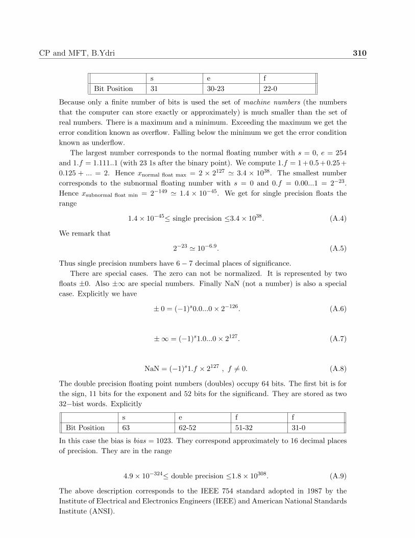
CP and MFT, B.Ydri 310
s e f
Bit Position 31 30-23 22-0
Because only a finite number of bits is used the set of machine numbers (the numbers
that the computer can store exactly or approximately) is much smaller than the set of
real numbers. There is a maximum and a minimum. Exceeding the maximum we get the
error condition known as overflow. Falling below the minimum we get the error condition
known as underflow.
The largest number corresponds to the normal floating number with s = 0, e = 254
and 1.f = 1.111..1 (with 23 1s after the binary point). We compute 1.f = 1 + 0.5 + 0.25 +
0.125 + ... = 2. Hence xnormal float max = 2 × 2127 ' 3.4 × 1038. The smallest number
corresponds to the subnormal floating number with s = 0 and 0.f = 0.00...1 = 2−23.
Hence xsubnormal float min = 2−149 ' 1.4 × 10−45. We get for single precision floats the
range
1.4× 10−45≤ single precision ≤3.4× 1038. (A.4)
We remark that
2−23 ' 10−6.9. (A.5)
Thus single precision numbers have 6− 7 decimal places of significance.
There are special cases. The zero can not be normalized. It is represented by two
floats ±0. Also ±∞ are special numbers. Finally NaN (not a number) is also a special
case. Explicitly we have
± 0 = (−1)s0.0...0× 2−126. (A.6)
±∞ = (−1)s1.0...0× 2127. (A.7)
NaN = (−1)s1.f × 2127 , f 6= 0. (A.8)
The double precision floating point numbers (doubles) occupy 64 bits. The first bit is for
the sign, 11 bits for the exponent and 52 bits for the significand. They are stored as two
32−bist words. Explicitly
s e f f
Bit Position 63 62-52 51-32 31-0
In this case the bias is bias = 1023. They correspond approximately to 16 decimal places
of precision. They are in the range
4.9× 10−324≤ double precision ≤1.8× 10308. (A.9)
The above description corresponds to the IEEE 754 standard adopted in 1987 by the
Institute of Electrical and Electronics Engineers (IEEE) and American National Standards
Institute (ANSI).
CP and MFT, B.Ydri 311
Machine Precision and Roundoff Errors: The gap ε between the number 1
and the next largest number is called the machine precision. For single precision we get
ε = 2−23. For double precision we get ε = 2−52.
Alternatively the machine precision εm is the largest positive number which if added
to the number stored as 1 will not change this stored 1, viz
1c + εm = 1c. (A.10)
Clearly εm < ε. The number xc is the computer representation of of the number x. The
relative error εx in xc is therefore such that
|εx| = |xc − xx|≤εm. (A.11)
All single precision numbers contain an error in their 6th decimal place and all double
precision numbers contain an error in their 15th decimal place.
An operation on the computer will therefore only approximate the analytic answer
since numbers are stored approximately. For example the difference a = b − c is on the
computer ac = bc − cc. We compute
aca
= 1 + εbb
a− εc
c
a. (A.12)
In particular the subtraction of two very large nearly equal numbers b and c may lead to
a very large error in the answer ac. Indeed we get the error
εa 'b
a(εb − εc). (A.13)
In other words the large number b/a can magnify the error considerably. This is called
subtractive cancellation.
Let us next consider the operation of multiplication of two numbers b and c to produce
a number a, viz a = b× c. This operation is represented on the computer by ac = bc× cc.We get the error
εa = εb + εc. (A.14)
Let us now consider an operation involving a large number N of steps. The question we
want to ask is how does the roundoff error accumulate.
The main observation is that roundoff errors grow slowly and randomly with N . They
diverge as N gets very large. By assuming that the roundoff errors in the individual steps
of the operation are not correlated we can view the accumulation of error as a random
walk problem with step size equal to the machine precison εm. We know from the study
of the random walk problem in statistical mechanics that the total roundoff error will be
proportional to√N , namely
εro =√Nεm. (A.15)
This is the most conservative estimation of the roundoff errors. The roundoff errors are
analogous to the uncertainty in the measurement of a physical quantity.
CP and MFT, B.Ydri 312
Systematic (Algorithmic) Errors: This type of errors arise from the use of ap-
proximate numerical solutions. In general the algorithmic (systematic) error is inversely
proportional to some power of the number of steps N , i.e.
εsys =α
Nβ. (A.16)
The total error is obtained by adding the roundoff error, viz
εtot = εsys + εro =α
Nβ+√Nεm. (A.17)
There is a competition between the two types of errors. For small N it is the systematic
error which dominates while for large N the roundoff error dominates. This is very
interesting because it means that by trying to decrease the systematic error (by increasing
N) we will increase the roundoff error. The best algorithm is the algorithm which gives
an acceptable approximation in a small number of steps so that there will be no time for
roundoff errors to grow large.
As an example let us consider the case β = 2 and α = 1. The total error is
εtot =1
N2+√Nεm. (A.18)
This error is minimum when
dεtot
dN= 0. (A.19)
For single precision calculation (εm = 10−7) we get N = 1099. Hence εtot = 4 × 10⁻⁶.
Most of the error is roundoff. In order to decrease the roundoff error and hence the total
error in this example we need to decrease the number of steps. Furthermore in order for
the systematic error to not increase when we decrease the number of steps we must find
another algorithm which converges faster with N . For an algorithm with α = 2 and β = 4
the total error is
εtot =2
N4+√Nεm. (A.20)
This error is minimum now at N = 67 for which εtot = 9 × 10⁻⁷. We have only 1/16 as
many steps with an error smaller by a factor of 4.

Appendix B
Executive Arabic Summary of
Part I

T§ d` ºA§zyf ¨TyqybW Am
©Cd§ H§ A
r¶z ,TAn ,CAt ¨A T`A ,ºA§zyf dh`
2015 ¨fA
308

xrhf
310 . . . . . . . . . . . . . . . . . . . . . . . . . . . . . . . . . . . . . . . . . . . . . . . . . Tdq 0
312 . . . . . . . . . . . . . . . . . . . . . . . . . . . . . . . . . ºwh T¤Aq -r¤ TyECw 1
313 . . . . . . . . . . . . . . . . . . . . . . . . . . ºwh T¤Aq ry ¶@q Tr 2
314 . . . . . . . . . . . . . . . . . . ¯ry ¤ r¤r -r¤ AyECw -¨qwt Ezh 3316 . . . . . . . . . . . . . . . . . . . . . . . . . . . . . . . . . . . . . . . . . . T§ d` ®Akt 4317 . . . . . . . . . . . . . . . . . . . . . . . . . . . . . . . . . . . wsC - wy AyECw 5
318 . . . . . . . . . . . . . . . . . . . . . . . TysmK Twmm -Aw - ¤C TyECw 6
320 . . . . . . . . . . . . . . . . . . . . . . CAW wk ¨smK yS C¤ Ts 7
322 . . . . . . . . . . . . . . . . . . . . . . . . . . . . . . TJrf ry : 1 ©wRwf xwn 8324 . . . . . . . . . . . . . . . . . . . . . . . . . . . . . ©rkw VAq : 2 ©wRwf xwn 9326 . . . . . . . . . . . . . . . . . . . . . . . . C¤d AS r¡AZ : 3 ©wRwf xwn 10327 . . . . . . . . rZAntl ¨¶Aqlt CAsk¯ ¤ CAWK¯ AWW :4 ©wRwf xwn 11330 . . . . . . . . . . . . . . . . . . . . . . . . . . §wsA §Ew :1 ¨·§z yAn§d 12332 . . . . . . . . . . . . . . . . . . . . . . . . . . . . . . . CAhO¯ :2 ¨·§z yAn§d 13333 . . . . . . . . . . . . . . . . . . . . . . . . . . . . . . . . . . . . . . . . . Ty¶wK` d¯ 14334 . . . . . . . . . . . . . . . . . . . . . . . . . . . . . . . . . . . . . . . . . . ¨¶wK` ºAKm 15335 . . . . . . . . . . . . . . . . . . . . . . . . . wCA ¨tw ¤ ¨WFw TWqn Ab§rq 16337 . . . . . . . . . . . . . . . . . . . . . . . . . . . . . . . Tm\tnm ry Amt¯ A`§Ew 17339 . . . . . . . . . . . . . . . . . . . . . . . . . . n§z§ Ðwm ¤ Hyw¤rty TyECw 18
341 . . . . . . . . . . . . . . . . . . . ¨syVAn¤ryf TyA Tbr ©CwW ryt 19342 . . . . . . . . . . . . . . . . . . . . . . . . . . . . . . . . . . . Ty¶An (§r) Xr T 20
344 . . . . . . . . . . . . . . . . . . . . ¨¤¯ Tbr ©CwW ryt ¤ Hys§rtsh 21
309

CP and MFT , B . Ydri310
Tdq
¤ Tyml` TywFA FA AS§ r` ¨t T§ d` wl` ¤r d ¨¡ T§ d` ºA§zyfAywwnkt ¨ O ©@ ¶Ah dqt ry¯ TnF 30− 40 ® Cwlb ¤ rhZ ¨t
.Tyk§r¯ dtm A§¯w ¨ TA TymrXr§ rs A¡CAbt km§ ¤ T§r\n ºA§zyf As s T§ d` ºA§zyf CAbt km§Td ¶A PO A¡rbt`§ ¨t An¡ ¤ Tyb§rt ºA§zyf ¤ T§r\n ºA§zyf y,wy rO @n ¯ ¨l , AtlAkt AtCAq An¡ A§dylq .s ¯ Tyb§rt ºA§zyfAn¡ .Tyb§rt TCAqm An¡ ©r TyA ¤ T§r\n TCAqm TyA Anh .ºA§zyflTA TCAq dw ¢ rbt`§ ,¡ry ¤ Am @¡ ¨ ylA` TA , ¯ ryk¨¡ T§ d` ºA§zyf A £@¡ r\n Th¤ .T§ d` TCAqm ¨¡ ºA§zyfl Tflt ¤ TlOfnTh¤ A @¡ C .¨b§rt ¤ ©r\n ylqA C¤rSA Xbr ry ¢@ Ofn qw¡ T§ d` ºA§zyf rbt`§ ©@ ¤¯ ©r w¡ T§wWm £@¡ ¨ A¡Anbt wF ¨t r\n
.T§r\n ºA§zyf ¤r r rAn ¤ T§r\n ºA§zyf TA ¤ ºA§zyf rAn z t§ T§ d` ºA§zyf ¨ Trb wFA wl rAn © d` ylt TyqybWt AyRA§r
.¤r` ¤ A Ah Hy Tny` Ty¶A§zy TAs w¡ d¤ d¡.T§ d` (AA m) AyAm ºr w¡ ºA§zyf ¨ rwybmk ¯Am`tF ¡ry TyRA§C ¯ A` Ahy kt ¨t Ty¶A§zyf ¶Asm r ¶® T§ d` AyAmT§ d AA ©¯ ºdb TWq .ªwbS ¨lyl ¨l Ahm\` ¨ rwt ¯ ¨t ¤ TyW A Ð A dt d§r An ¨`ybW ¤ TFCd dy Ty¶A§zyf Tlml ¨A Ðwm w¡¨ A TCAqml Tyb§r ¶At rw TA ¨ ¯ ¤ d¡AKm sn Ðwmn @¡ rOA Ð Trt ¢yW` km§ A rKtF w¡ dh A Tyb§r ¶At © rw d TAEA TyRA§C TyECw A§ w¡ dh @¡ yq ¨¤¯ wW . §r¢yms A w¡ rwybm ¨l EA¯ @¡ @yfn .rwybmk ¨l AS§ ¤ A§r\ Ðwmn @¡©dA Twtk rfJ ¨ TyRA§r TyECw Tmr ¨l dmt`§ w¡ ¤ T§ d` AAmA
.Ahmhf§ rwybmkl km§ Trb AAAm ¨ ¨RA§r Ðwmn `l§ ®m .TyRrt CA Ð ¨¡ T§ d` AyAmAhlm`ts ¨t rfK¤ TyECw A Tylm`m Trt ¨ Tny` C¤ XbSA T§ d`Am`tF ¨ ºdb b .Tylm`m Trt ¨ xAyq EAh C¤d wq ¨h T§ d` AAmAn Am AAm rfK r§A` ¤ CAbt Anyl ¢A Ty¶A§zyf TFCd ¨ T§ d` AAm©@ xAyq .xAy © ºr ¨ ºdb b Tylm`m Trt ¨ xAyq EAh r§A`m wq® tt ¤ T§ d` AAm ¢§r ©@ As ¢lAq§ Tylm`m T§rt ¨ ¢ wq
.AyW`m yl w¡ ¤ r± Hfn ytylm`\` ¨ .Trb A ¨¡ T§ d` ºA§zyf ¶AF¤ ¡ ¨`ybW ¤ d Rw Al ©d ¨ rfK tk Ty¶A§zyf Tyb Am¯ ¨ A¡d ¨t T§ d` AyAmTA dn AS§ km§ AyAm £@¡ ¨ .(𝐶) ¨F T ¤ (Fortran) ¤rrf T`mmT§ d` Ayrb Am`tF .A¡ry ¤ (Lapack) A¯ T§ d` Any¤r Abtk AnTA ,T§ d` AyAm £@¡ ¨ (Mathematica) AkyAmyA ¤ (Matlab) ®A z¡AE ¨ © ¥§ ¢¯ rmA ¨lm ry ,(Monte Carlo) wCA ¨twm Tq§rV ¨l dmt` ¨t

CP and MFT , B . Ydri311
z¡A Ayrb w ¨ QwOA C @¡ ¤ rwybmk ¨l rfKl d §wV ryFdyf z¡A Ayrb ¨ J ¨ An¡ Hy .T`m A sy ¤ Tmrt A ¨¡AyAm ¨ AAm Tm¶® ry Ahnk Crkt ¨l dmt` ¯ ¨t T§ d` AAs ¨ T§AlT§wWm £@¡ ¨ .rm ¶A¡ d wW Hf Crk ¨l xAF¯A dmt` ¨t T§ d`dtF nt ¤ T`m T ¨ AnrfJ ym tk wF © §rW @¡ XbSA bt wFHkyny yKt A\ ¨l 90 ¤ 77 ¤rrf QwOA dts wF .z¡A Ayrb
. (Ubuntu) wtnw§ §Ew (Linux)ºA§zyf rRAm Tqrm TyqybWt Am¯ wm ¨l ©wt T§wWm £@¡TblV ¨l 2009 A` @n ºA§zyf dh` ¨ ©Cd§ H§ A ¥m A¡Aq ¨t T§ d`T§ d` ºA§zyf ,(ºA§zy HAsy) © d` ylt Hy§Aq CAV ¨ rtFAm ¤ HAsyl¨l wO km§ .(rtFAm AOO ¨A) ¨¯ ®¯ ¤ (T§r\ ºA§zy rtFA)rb ©Cd§ H§ A ¥mA AO¯ §rV -T§ d` ºA§zyf ¨ rRAm- T§wW¨l ¢tA ¨mFr wm fO ¤ badis.ydri@univ − annaba.org ¨¤rtk¯ d§rb
.http : //homepages.dias.ie/ydri/
rkKA m` §r ¨A ¤ ¢sf TA ©Cd§ H§ A ¥m dqt§ At ¨¨A r§dml @ ¤ AhJ ¨fWO ÐAtF¯ ºA§zyf dh`m As r§dml §z T§db @n A¡Ad ¨t ryk ®yhst ¤ Tlyl dAsml ¨AbyJ ¤® ÐAtF¯
.ºA§zyfl TymFr rb ¨ AqybWt ¤ rRAm £@¡ A
©Cd§ H§ Ar¶z ,TAn ,©d§rF2013 Tyl§w 8 yn¯

CP and MFT , B . Ydri312
ºwh T¤Aq -r¤ TyECw
AhqbW§ ¨t wq . 𝑣 Trs TWs ¤ Tmyqts §rV ¨l Ty¶w¡ TC ¨RA§C wq§TynE rtf ¨RA§r A¡rw§ ª¤ 200 ©¤As 𝑃 TtA TAWtF ¸Ak TCd ¨l ¨RA§rTsA` wk (¨¶wh r wq AS§ r` ¨t) ºwh T¤Aq w .d¤ TAs Cdq
T®`A AW` Trs r rV TbFAnt ¤ Trl
𝐹drag = −𝐶𝜌𝐴𝑣2.
¨Rr` Wqm TAs ¨¡ 𝐴 ¤ r A` w¡ 𝐶 ,ºwh TA ¨¡ 𝜌 T A`m £@¡ ¨¨At kK @§ ¨A wy wA .TCd d¶E ¨RA§r Tlm
𝑑𝑣
𝑑𝑡=
𝑃
𝑚𝑣− 𝐶𝜌𝐴𝑣2
𝑚.
¨l dmt` Tsm £@h T§ d` TCAqm .z ¨ Td 𝑣 Trs As w¡ wlWmry ¨nE A 𝑁 ¨ 𝑇 ¨nz Am Wq .r¤ TyECw
Δ𝑡 =𝑇
𝑁
©𝑡 = 𝑖Δ𝑡 , 𝑖 = 0, ..., 𝑁.
r`𝑣(𝑖) = 𝑣(𝑡−Δ𝑡).
kK @§ r¤ §rqt ¨W`m
𝑣(𝑖+ 1) = 𝑣(𝑖) + Δ𝑡
(𝑃
𝑚𝑣(𝑖)− 𝐶𝜌𝐴𝑣2(𝑖)
𝑚
). 𝑖 = 1, ..., 𝑁 + 1
¨W` Tqrm Tynz A\l
𝑡(𝑖+ 1) = 𝑖Δ𝑡 , 𝑖 = 1, ..., 𝑁 + 1.
w¤ d TA ¨¤ ºwh T¤Aq w¤ TA ¨ z ¨ Td Trs s (1)AS§ ¨W` .0.5 ©¤As§ 𝐶 r A @ ¥s @¡ ¨ .^® ÐA .ºwh T¤Aq
yq𝑚 = 70kg , 𝐴 = 0.33𝑚2 , 𝜌 = 1.2kg/𝑚3 , Δ𝑡 = 0.1𝑠 , 𝑇 = 200𝑠.
¨W` Ty¶dt¯ Trs𝑣(1) = 4𝑚/𝑠 , 𝑡(1) = 0.
ryO t§ Adn ^® ÐA .TAWtF¯ ¤/¤ r A ryy TA ¨ ^® ÐA (2)
.Tynz wW

CP and MFT , B . Ydri313
ºwh T¤Aq ry ¶@q Tr
wk ¤ Tr £A Hk m` ¨t ºwh T¤Aq w ry Tf§@ Tr rbt`¯ A` ¨ © ¥§ ¨A wy wA .𝐵 FAnt A zr .Trs r TbFAnt
TyAt Tr𝑑𝑥
𝑑𝑡= 𝑣𝑥 , 𝑚
𝑑𝑣𝑥𝑑𝑡
= −𝐵𝑣𝑣𝑥.
𝑑𝑦
𝑑𝑡= 𝑣𝑦 , 𝑚
𝑑𝑣𝑦𝑑𝑡
= −𝑚𝑔 −𝐵𝑣𝑣𝑦.
¨At kK @ r¤ TyECw ¨W`m TylRAft ¯ A`m £@¡
𝑣𝑥(𝑖+ 1) = 𝑣𝑥(𝑖)−Δ𝑡𝐵𝑣(𝑖)𝑣𝑥(𝑖)
𝑚.
𝑣𝑦(𝑖+ 1) = 𝑣𝑦(𝑖)−Δ𝑡𝑔 −Δ𝑡𝐵𝑣(𝑖)𝑣𝑦(𝑖)
𝑚.
𝑣(𝑖+ 1) =√𝑣2𝑥(𝑖+ 1) + 𝑣2𝑦(𝑖+ 1).
𝑥(𝑖+ 1) = 𝑥(𝑖) + Δ𝑡 𝑣𝑥(𝑖).
𝑦(𝑖+ 1) = 𝑦(𝑖) + Δ𝑡 𝑣𝑦(𝑖).
.𝑁 ¨ 1 yq @§ 𝑖 ¤ 𝑖 1 Tmyq w Trs ¤ Rwml Ty¶dt¯ yq.Tsm r¤ TyECw ¨W`m Ahy zn ¤rCw rfJ t (1)
TyAt yq @ (2)𝐵
𝑚= 0.00004𝑚−1 , 𝑔 = 9.8𝑚/𝑠2.
𝑣(1) = 700𝑚/𝑠 , 𝜃 = 30 degree.
𝑣𝑥(1) = 𝑣(1) cos 𝜃 , 𝑣𝑦(1) = 𝑣(1) sin 𝜃.
𝑁 = 105 , Δ𝑡 = 0.01𝑠.
.^® ÐA .ºwh T¤Aq ¤ ¤d CAsm s
Tql AS§ §rOt @¡ .Tf§@q ©d yy` km§ 𝑖𝑓 ¨VrK §rOt dtFA (3)
¨AtA 𝑑𝑜
if(𝑦(𝑖+ 1).le.0)exit.
.ºwhl T¤Aq w¤ d TA ¨ ¤ w¤ TA ¨ Tf§@q ©d y
T§¤z wk Am ¢ Tmy \ @§ ©dm r` ºwhl T¤Aq w¤ d TA ¨ (4)
.Ty¶dt¯ T§¤zl y d CAbtA A§ d r¯ @¡ q .TC 45 ©¤As Ty¶dt¯ b ¤ T§¤z ¨ Td ©dm TFC T§¤z ¨ 𝑑𝑜 Tql TAR AS§ km§
.¨m\` ¢tmy
.¨m\ ©dm Ahy wk§ ¨t T§¤z s ºwh T¤Aq w¤ TA ¨ (5)
CP and MFT , B . Ydri314
¯ry ¤ r¤r -r¤ AyECw -¨qwt Ezh
A zkr ¨ l` 𝑙 ¢wV Xy TVwr 𝑚 Tlt CAb Xys ¨qw Ez¡ rbt`Cwm xwn Ah`nO§ ¨t T§¤z © TyW Tr |rtf .𝑔 TAq ry
kK @ ¨A wy wA TqtKm Ezt¡¯ T A` .£ry Am¶ ¨qb ¨wAK𝑑2𝜃
𝑑𝑡2+
𝑔
𝑙𝜃 = 0.
Tbr ytylRAf yt A`m AhS§w` km§ ¢yA ¢br TylRAft T A`m £@¡¨AtA ¨¤¯
𝑑𝜃
𝑑𝑡= Ω ,
𝑑Ω
𝑑𝑡= −𝑔
𝑙𝜃.
r¤ TyECw ¨W`m w¡ An¡ £rbt`nF ©@ ¤¯ © d`
Ω𝑖+1 = Ω𝑖 −𝑔
𝑙𝜃𝑖 Δ𝑡.
𝜃𝑖+1 = 𝜃𝑖 + Ω𝑖 Δ𝑡.
@¡ .r¤r -r¤ TyECw ¨W`m w¡ An¡ £rbt`nF ©@ r¯ © d` TyAt ¯ A`mA ¨W`§
Ω𝑖+1 = Ω𝑖 −𝑔
𝑙𝜃𝑖 Δ𝑡.
𝜃𝑖+1 = 𝜃𝑖 + Ω𝑖+1 Δ𝑡.
kK @§ ©@ ¯ry TyECw ¨W`m AS§ An¡ rbt`
𝜃𝑖+1 = 2𝜃𝑖 − 𝜃𝑖−1 −𝑔
𝑙𝜃𝑖(Δ𝑡)2.
r¤r -r¤ ¤ r¤ AyECw AW`m wl Ahy zn ¤rCw rfJ t (1).¨qwt Ezh Tsm
¨W` Ezh TAV .z ¨ ¤d TAW ¤ T§¤z Trs ,T§¤z s (2)
𝐸 =1
2Ω2 +
1
2
𝑔
𝑙𝜃2.
T§ d` yq @𝑔 = 9.8𝑚/𝑠2 , 𝑙 = 1𝑚 .
Tynz wW ¤ wW d @𝑁 = 10000 , Δ𝑡 = 0.05𝑠.
Aty¶dt¯ T§¤z Trs ¤ T§¤z @𝜃1 = 0.1radian , Ω1 = 0.
¨AtA C¤d A`R Tsm Tr E d§d km§ 𝑖𝑓 ¨VrK §rOt Am`tFAif(𝑡(𝑖+ 1).ge.5 * period) exit.

CP and MFT , B . Ydri315
ÐA .r¤r -r¤A Twsm TAW Tmy ¤ r¤A Twsm TAW Tmy y CA (3)
.tnts ÐA ¤ ^®
®W¯ Ahnkm§ ¯ Tq§rW £@¡ ^®n .¯ry TyECw dtFA As d (4)Am`tFA AhAs km§ ¨t 𝜃2 T§¤z ºAW AS§ § . Ω1 ¤ 𝜃1 Ty¶dt¯ yq Xq
© r¤ Tq§rV𝜃2 = 𝜃1 + Ω1 Δ𝑡.
k .T§¤z Trs As ¨ At ¯ ¯ry TyECw AS§ ^®nCAb` Am`tFA Ahbs ¨t T§¤z Trs Tr` ¨ At TAW As
Ω𝑖 =𝜃𝑖+1 − 𝜃𝑖−1
2Δ𝑡.

CP and MFT , B . Ydri316
T§ d` ®Akt
kK d¤ d` ¨ ®Akt rbt`
𝐼 =
∫ 𝑏
𝑎
𝑑𝑥𝑓(𝑥).
CAy w¡ © d` ¨qb§ ¤ Aylyl Akt ºr Ahy km§ ¯ ¨t TA` TA rbt`¤ rnm £AbJ ¤ ®yWtsmA §rqt ¨¡ Ahlm`tsnF ¨t AyECw . dyw
Δ𝑥 ¢wV A 𝑁 ¨ §r`t A sq rW £@¡ ¨ . ¸Akm wWq §rqt¨AtA
𝑥𝑖 = 𝑥0 + 𝑖Δ𝑥 , 𝑖 = 0, ..., 𝑁 , Δ𝑥 =𝑏− 𝑎
𝑁, 𝑥0 = 𝑎, 𝑥𝑁 = 𝑏.
¨W`§ ®yWtsmA §rqt
𝐹𝑁 = Δ𝑥
𝑁−1∑
𝑖=0
𝑓(𝑥𝑖).
¨W`§ rnm £AbJA §rqt
𝑇𝑁 = Δ𝑥
[1
2𝑓(𝑥0) +
𝑁−1∑
𝑖=1
𝑓(𝑥𝑖) +1
2𝑓(𝑥𝑁)
].
(¨¤E wk§ § 𝑁 An¡ ) ¨W`§ ( wsbmyF dA) ¸Akm wWq §rqt
𝑆𝑁 =Δ𝑥
3
[𝑓(𝑥0) + 4
𝑁−22∑
𝑖=0
𝑓(𝑥2𝑖+1) + 2
𝑁−22∑
𝑖=0
𝑓(𝑥2𝑖) + 𝑓(𝑥𝑁)
].
. ¨wt ¨l 1/𝑁4 ¤ 1/𝑁2 ,1/𝑁 FAnt ® Ab§rqt £@¡ ¨ W
Akt @ (1)
𝐼 =
∫ 1
0
𝑓(𝑥)𝑑𝑥 ; 𝑓(𝑥) = 2𝑥+ 3𝑥2 + 4𝑥3.
.Tylylt Akt Tmy CA .®yWtsm Tq§rV Am`tFA Akt @¡ Tmy s. function ¤ subroutine Am`tFA Td rfJ :T\®
.©r\n CA .𝑁 T¯d krm W s . 𝑁 ¯Am d ry (2)
. wsbmyF dA ¤ rnm £AbJ Tq§rV Am`tFA yqAs y¥s d (3)
TyAt ®Akt ¯ @ (4)
𝐼 =
∫ 𝜋2
0
cos𝑥𝑑𝑥 , 𝐼 =
∫ 𝑒
1
1
𝑥𝑑𝑥 , 𝐼 =
∫ +1
−1
lim𝜖−→0
(1
𝜋
𝜖
𝑥2 + 𝜖2
)𝑑𝑥.
CP and MFT , B . Ydri317
wsC - wy TyECw
th .+𝑎 ¨ −𝑎 dtm§ 2𝑎 ¢wV ¤ 𝑉 ¢AfC wm r· ¨ rt§ 𝑚 Tlt ¤Ð ysd Tlm TA .TWbrm ¯A © r·b AfC r¯ AAW Ð Tlm ¯A
wl ¨W` Ty¤z Tywm ¤dA Tqrm Ah wmsm AAW .T§ r ¤ Ty¤E wkTyAstm T A`m
𝛼 tan𝛼𝑎 = 𝛽.
𝛼 =
√2𝑚𝐸
~2, 𝛽 =
√2𝑚(𝑉 − 𝐸)
~2.
wl d ¨¶Ah® wmk r· TA ¨
𝐸𝑛 =(𝑛+ 1
2)2𝜋2~2
2𝑚𝑎2, 𝑛 = 0, 1....
(dw TAt Am¡ )CAt~ = 1 , 𝑎 = 1 , 2𝑚 = 1.
© C¤@ A§A An ms ¨t wsC - wy TyECw m`ts 𝐸 AAW A§ TWqn 𝑓(𝑥) = 0 T A`m rq AnA 𝑥0 y` ym A®W .¨AtA 𝑓(𝑥) = 0 T A`
w¡ ¤ 𝑥1 ¤¯ §rqt @¡ ¨ms .Anys Cw 𝑥0 TWqn ¨ 𝑓(𝑥) Td xAm VAqT A`mA ¨W`§
𝑥1 = 𝑥0 −𝑓(𝑥0)
𝑓 ′(𝑥0).
𝑥2 dts 𝑥2 ¨A §rqt A§ wW Hfn wq 𝑥1 A®WT®`A 𝑥𝑖 §rqt T¯d ¨W`§ 𝑥𝑖+1 §rqt .@k¡ ¤ 𝑥3 A §rqt A§
𝑥𝑖+1 = 𝑥𝑖 −𝑓(𝑥𝑖)
𝑓 ′(𝑥𝑖).
ytd TFC rb TyAyb Tq§rW Am`tFA 𝐸 wl d y 𝑉 = 10 (1)
𝑓(𝛼) = tan𝛼𝑎 , 𝑔(𝛼) =𝛽
𝛼=
√𝑉
𝛼2− 1.
A§ .10−8 ©¤As ¤ Td yl wsr-wy Tq§rV Am`tFA d (2)
Td ¨¤¯ dAbt TWq ¨ wsr-wy Tq§rW ¤¯ ymt @ ¤¯ TyA dAbt TWq ¨ ¤¯ ymt @ ¨A A§ .𝛼 = 𝜋/𝑎 © \
.𝛼 = 2𝜋/𝑎 ©
. 𝑉 = 20 ¥s d (3)
ymt d§d TyAyb Tq§rWA `tF .𝑉 = 100 T`C¯ wl d (4)
.r ¤¯
.yOnt Tq§rV Am`tFA TqAs Tl·F¯ d (5)

CP and MFT , B . Ydri318
TysmK Twmm -Aw - ¤C TyECw
Tlt |rtf .HmK w rt§ d¤ w TlkK TysmJ Twm rbt`zr ¨ TnAF A¡CAbt km§ y wk Tlt TCAqmA d Tlyq HmK
TyAt Tr ¯ A` ¨W`§ ¨A wy wA .A\n
𝑣𝑥 =𝑑𝑥
𝑑𝑡,𝑑𝑣𝑥𝑑𝑡
= −𝐺𝑀𝑠
𝑟3𝑥 , 𝑣𝑦 =
𝑑𝑦
𝑑𝑡,𝑑𝑣𝑦𝑑𝑡
= −𝐺𝑀𝑠
𝑟3𝑦.
𝑟 =√
𝑥2 + 𝑦2.
y Tyklf dw dts𝐺𝑀𝑠 = 4𝜋2𝐴𝑈3/𝑦𝑟2.
kK @§ Aw -¤C TyECw ¨W`m r@ Tf¯ Tr ¯ A`
𝑘1 = Δ𝑡 𝑣𝑥(𝑖) , 𝑝1 = Δ𝑡 𝑣𝑦(𝑖).
𝑟(𝑖) =√
𝑥(𝑖)2 + 𝑦(𝑖)2.
𝑘3 = −𝐺𝑀𝑠
𝑟(𝑖)3𝑥(𝑖)Δ𝑡 , 𝑝3 = −𝐺𝑀𝑠
𝑟(𝑖)3𝑦(𝑖)Δ𝑡.
𝑘2 = (𝑣𝑥(𝑖) +1
2𝑘3)Δ𝑡 , 𝑝2 = (𝑣𝑦(𝑖) +
1
2𝑝3)Δ𝑡.
𝑅(𝑖) =
√(𝑥(𝑖) +
1
2𝑘1)2 + (𝑦(𝑖) +
1
2𝑝1)2.
𝑘4 = −𝐺𝑀𝑠
𝑅(𝑖)3(𝑥(𝑖) +
1
2𝑘1)Δ𝑡 , 𝑝4 = −𝐺𝑀𝑠
𝑅(𝑖)3(𝑦(𝑖) +
1
2𝑝1)Δ𝑡.
𝑥(𝑖+ 1) = 𝑥(𝑖) + 𝑘2.
𝑣𝑥(𝑖+ 1) = 𝑣𝑥(𝑖) + 𝑘4.
𝑦(𝑖+ 1) = 𝑦(𝑖) + 𝑝2.
𝑣𝑦(𝑖+ 1) = 𝑣𝑦(𝑖) + 𝑝4.
w Trs ¤ Rwml Ty¶dt¯ yq . 𝑁 ¨ 1 yq @§ 𝑖 TqAs ¯ A`m ¨.𝑖 1 Tmyq
A\n Tsm Aw - ¤C TyECw ¨W`m Ahy zn ¤rCw rfJ t (1).¨smK
.TAWl TbsnA ^® ÐA .z ¨ ¤d TAW @ ¤ Trs ¤ CAsm s (2) ¨W` Tltk d¤ ¨ wk TAV A ry@tl .Tyklf dw dtF
𝐸 =1
2𝑣2 − 𝐺𝑀𝑠
𝑟.

CP and MFT , B . Ydri319
d ¨ HmK w¤ TOA wW ¨¡ Cdm ym A ¤¯ rlb wA s (3)
T§r¶ AhCd d¡AKm l` ¨t wk Xq rbt`nF ¨l§ A ¨ .yrmAO . CwAF ¤ ©rtKm ¤ §rm ¤ |C¯ ¤ r¡z ¨¡ wk £@¡ .ryb d ¨
Tyklf dw d¤ ¨ ¨W` CAW¯
𝑎venus = 0.72 , 𝑎earth = 1 , 𝑎mars = 1.52 , 𝑎jupiter = 5.2 , 𝑎saturn = 9.54.
.wk £@¡ ¤¯ rlb wA qTy¶dt¯ ª¤rK @ 3 ¤ 2 yqAs y¥s ¨l TA¯
𝑥(1) = 𝑎 , 𝑦(1) = 0 , 𝑣𝑥(1) = 0 , 𝑣𝑦(1) = 𝑣.
¤ yO CAsm ¨l wO d Tmh Ty¶dt¯ Trs A¡@ ¨t Tmyq¨Aq @ w A ¨AtA ¤ ©r¶ ®` w¡ CAsm |rt ® Ahnyy` t§
¨l O .©zrm rW w TEwt wk
𝑣 =
√𝐺𝑀𝑠
𝑎.
¨¯A Crkt d ¤ Tynz wW @AS§
Δ𝑡 = 0.01𝑦𝑟 , 𝑁 = 103 − 104.
.rWq O `k rV FAnt wk§ C¤d r A A rlb wA s (4)
r¯ @¡ q .d¤ XbSA ©¤As§ FAnt A A T§r¶d Cdm wk r§ ¨t Tbrm ® C¤d xAy t§ .£® Cw@m wk
.HmK ¢ TWq d` ¨
r .PA W Cd ¨l wO km§ ¢A TbFAn Tq§rW Ty¶dt¯ Trs ryyt (5)
.r¯ @¡
@¡ ¨ £Arbt ©@ Xsbm ¨smK A\n Tr Amk§ @ AyFAF¯ AwAq (6) ¨A wy wA ¤ Th tk y ¨Aq @l wy wA w¡ §rmt
.©rThT§zr wk ¤ HmK y wq ¨ £ wn ¡ ¨ Pn§ ¨Aq @ wA ¨¯ ¨ |rtf .TAsm r Ask TbFAnt ¤ HmK w wk ThwrfK ry .yn lt TAsml r x Ask TbFAnt ¨¡ ¨Aq @ wAFAF Cdm s .CAbt¯ y` wql d§d rOt @¡ @
.tnts ÐA ¤ ^® ÐA .d¤ ¤ T® y

CP and MFT , B . Ydri320
CAW wk ¨smK yS C¤ Ts
¨W` CAW AhnmR ¤ CAys wk ym Cd A ¤¯ rlb wA sybW ¢AqtJ km§ wAq @¡ . yrm d ¨ HmK w¤ TOA wWq
wk Af Am¡ Annkm§ ¢ |rt HmK wk Af ¨l wy ywwWq C¤A C¤ r¡AZ ¨ © ¥§ `b AhS` ¨l wk ry . Ahny Amy Ahsf
TWq r w¡ ©@ HmK w ¨smK yS C¤ ¨ ¨AtA ¤ HmK w TOAnym d§ HmK w ¨smK ySl C¤d @¡ . HmK wk CAs ¨. ryb d ¨ T§r¶ ¨¡ Cdm l w bs T§Al Tb` ¢d¡AK k wk
A wwlb TbsnA k .ryb T§zr¯ Ð TOA wW Cd Ah CAW ¤ wwl Xqkm§ ©@ CAW ¨qb§ .¨smK ¢SyS C¤ d¡AKm ms ¯ TSfnm T§Cdm ¢trF
TyAt C¤d TrF xAyq wyklf A .rbt` Td HmK w ¢SyS C¤ xAy566 arcsecond/century.
¢A ©r Th .TnF 240000 HmK w TlA C¤ nO§ CAW yS ©¨A ry CAbt¯ y` @ HmK CAW w Af ¨l wy yw ybWt
C¤d TrF s CAW ¨l wk523 arcsecond/century.
w¡ rf43 arcsecond/century.
Ah ¨l TAql Anmh ® © TA` Tybsn ® ¯ A¡rysf km§ ¯ Tymk £@¡HmK Tlt bs z-ºASf ºAn TmAn £wq .z-ºASf ºAn AhWFwt§ w
Ahb§rq km§ wk £ry r CAW A¡r`Kts§ ¨t¤
𝐹 =𝐺𝑀𝑠𝑀𝑚
𝑟2(1 +
𝛼
𝑟2) , 𝛼 = 1.1.10−8𝐴𝑈2.
¨smK ySl C¤ Tym ¨ ®` © ¥ wq £@¡ A§ d qt w¡ dh. rq ¨ TyA xw 43 ©¤As CAW`
CAbt¯ y` @¯ As ybWt ¨ A¡AndtF ¨t ¤rCwf rfJ d (1)
. £® Cw@m wqCAt . CAW Rw w¡ ¤¯ ¨¶dt¯ ªrK . T§Al h Ty¶dt¯ ª¤rK CAyt
𝑥0 = (1 + 𝑒)𝑎 , 𝑦0 = 0.
rWq O .HmK ¢ TWq d` ¨ Ty¶dt¯ T\l ¨ wk CAt An ©¨¡ 𝑒𝑎 TAsm . 0.206 ©¤As 𝑒 CAW T§zr¯ ¤ Tykl d¤ 0.39 w¡ CAW` 𝑎 rybk¨¶dt¯ ªrK . PAn Wq zr yrm d ¨ dw ¨t HmK d`
¨W` ¨t Ty¶dt¯ T\l ¨ CAW TrF w¡ ¨A
𝑣𝑥0 = 0 , 𝑣𝑦0 =
√𝐺𝑀𝑠
𝑎
1− 𝑒
1 + 𝑒.

CP and MFT , B . Ydri321
TAW _Af ¤ ¨r z` _Af ¨wA ybW AhAs km§ Trs £@¡ryO rWq S w¡ 𝑏 y (𝑥 = 0, 𝑦 = 𝑏) TWqn ¤ £® Ty¶dt¯ TWqn y
© CAW`𝑏 = 𝑎
√1− 𝑒2.
¨smK yS C¤ Tym A d £ry TA` Tybsn AhyW` ¨t 𝛼 ¢my ¯ (2)
Tmy CAt . ¤d ¤ Ð T§ d £AA © ¨ Aht\® `O§ Tly·R CAW`® 𝛼 ryk rb
𝛼 = 0.0008𝐴𝑈2.
AS§ CAt𝑁 = 20000 , 𝑑𝑡 = 0.0001.
CAW Xr§ ©@ A`K Ah`nO§ ¨t 𝜃 T§¤z s . yq £@¡ Cdm s¤ CAW ¤ HmK y TAsm AS§ s . z T¯d§ ¨q¯ Cwm HmK ¤
© zl TbsnA AhtqtK𝑑𝑟
𝑑𝑡=
𝑥𝑣𝑥 + 𝑦𝑣𝑦𝑟
.
TWq r l ¤ HmK ¢ TWq d` CAW l Aml AhCAJ ry TqtKm £@¡𝜃𝑝 T§¤z FC T\®m £@¡ dtF . HmK (¨smK yS ©) ¢
. ^® ÐA . z T¯d HmK ¢ TWq d` ¨ CAW wk§ AmHmK w CAW` ¨smK yS C¤ Tym XbSA w¡ ©@ 𝑑𝜃𝑝/𝑑𝑡 ym y
. £® CAtm 𝛼 Tmy
rtq . 𝛼 ©r y As ¥s d (3)
𝛼 = 0.001, 0.002, 0.004.
tntF . ym d¤ . ^® ÐA . 𝛼 T¯d 𝑑𝜃𝑝/𝑑𝑡 FC . 𝑑𝜃𝑝/𝑑𝑡 s r ¨Tmyq CAW` ¨smK yS C¤ Tym
𝛼 = 1.1.10−8𝐴𝑈2.
Td d¤ As ¥s AyW` dtFA (4)
𝑑𝜃𝑝𝑑𝑡
= 𝑓(𝛼).
. T§r¯ A`rm Tq§rV Am`tFA
CP and MFT , B . Ydri322
TJrf ry : 1 ©wRwf xwn
𝑔 TAq ry A zkr ¨ l` 𝑙 ¢wV Xy TVwr 𝑚 Tlt CAb xwCwm xwn Ah`nO§ ¨t T§¤z ¯ Awm TyW ry Tr ¨¡ xw © Tr .¤ −𝜋 ©rO Tmyq ¤ 𝜋 ¨m\` Tmyq lb km§¤ ry C¤rSA sy ¨wAK@ .£EAkC TWq w TC 360 ©¤As TlA C¤ C¤d§ km§ xwn A ¨AtAHwtF wAq ¨W` Ah |rtf¤ 𝑚 Tltk ¨l ºwh T¤Aq w ry CAbt¯ y`
𝑑𝜃/𝑑𝑡 Trs AyW TbFAnt ¤ Trl ¢sA` wk ºwh T¤Aq ¨l Pn§ ©@:𝑚𝑙𝑞 ©¤As§ FAn A
𝐹drag = −𝑚𝑙𝑞𝑑𝜃
𝑑𝑡.
xwn ®htF d`Tr ¢fw ¤ xwn Tr dA ¨ © ¥§ ºwh Akt¯©C¤rS ºwh T¤Aq dR xwn Tr ¨l _Af . Ty¶dt¯ ¢tAV AkTtA T`F ¤ 𝜈𝐷 rw Ð z ¨ T§C¤ w Ah |rtf ¨t TyCA §r w TAR
: 𝑚𝑙𝐹𝐷𝐹drive = 𝑚𝑙𝐹𝐷 sin 2𝜋𝜈𝐷𝑡.
kK @ ¨A wy wA TqtKm Ezt¡¯ T A`
𝑑2𝜃
𝑑𝑡2= −𝑔
𝑙sin 𝜃 − 𝑞
𝑑𝜃
𝑑𝑡+ 𝐹𝐷 sin 2𝜋𝜈𝐷𝑡.
. 𝑙 = 𝑔 © d¤ ©¤As§ xwnl TWysb Ezt¡¯A rm√𝑔/𝑙 ©¤z rwt Am¶ @
:r¤r - r¤ TyECw ¨W`m w¡ An¡ £rbt`nF ©@ © d`
Ω𝑖+1 = Ω𝑖 +
(− 𝑔
𝑙sin 𝜃𝑖 − 𝑞Ω𝑖 + 𝐹𝐷 sin 2𝜋𝜈𝐷𝑡𝑖
)Δ𝑡 , 𝜃𝑖+1 = 𝜃𝑖 + Ω𝑖+1 Δ𝑡.
zymt A ¡ ¤ (chaotic pendulum) ©wRwf xwn FA r` TykyAn§d Tlm £@¡TJrf ry FA AS§ r` TyA £@¡ . Ty¶dt¯ ª¤rKl TVrfm TyFAs ¢
. (butterfly effect)Ezhl TyW TqWnm ¨ . ytflt ytq§rW rOt§ ©wRwfEzhl km§
Tr Anlm¡ Ð TyCA §rt w C¤ ©¤As§ C¤ Ð T§C¤ Tr ©wRwfTAR¯A ¤ d Ahsf Crk ¯ T§C¤ ry Tr T§wRwf TqWnm ¨ . rA` Ty¶dt¯
¨ © ¥§ Ty¶dt¯ ª¤rK d§d ¨ rO ¨ £Ant A Amh W © A Ð ¨. AkA Tflt Tr
©wRwf Ezh Tsm r¤r -r¤ TyECw ¨W`m Ahy zn rfJ t (1)¨t TA ¨ ¤ [−𝜋, 𝜋] Am ¨ CwO A¡@ Am¶ km§ 𝜃 T§¤z ^®n .@¡ ¤ Am ¨ A¡rO A ±2𝜋 TARA wq Am @¡ CA Ahy wk
¨AtAif(𝜃𝑖.lt.∓ 𝜋) 𝜃𝑖 = 𝜃𝑖 ± 2𝜋.
CP and MFT , B . Ydri323
Ty¶dt¯ ª¤rK ¤ yq @ (2)
𝑑𝑡 = 0.04𝑠 , 2𝜋𝜈𝐷 =2
3𝑠−1 , 𝑞 =
1
2𝑠−1 , 𝑁 = 1000− 2000.
𝜃1 = 0.2 radian , Ω1 = 0 radian/𝑠.
𝐹𝐷 = 0 radian/𝑠2 , 𝐹𝐷 = 0.1 radian/𝑠2 , 𝐹𝐷 = 1.2 radian/𝑠2.
,TyCA§rt wq ¨¤¯ Tmyql TbsnA ^® ÐA .z T¯d 𝜃 T§¤z FCw¡A ,TyCA §rt wq TyA Tmyql TbsnA ^® ÐA .Ezt¡¯ rw w¡AÐA .TnE¯ ¨A Ezt¡¯ rw w¡A ¤ ©rO TnE¯ Ezt¡¯ rw
. T§C¤ Tr ¡ . TA Tmyql TbsnA ^®

CP and MFT , B . Ydri324
©rkw VAq : 2 ©wRwf xwn
TnE¯ ym ¨ Ezh rO ¯ Tymt Tr ¨¡ T§wRwf TqWnm ¨ Trkm§ ¯ k Tm¶® Ty¶dt ª¤rJ ºAW £® Tr T A` s§ Tq®Aht§¦C km§ TyA ¨¡ ¤ Ty¶wK Tlm w¡ ©wRwf Ezh ¨n`§ ¯ @¡ k .Ah ¥bnt
. ©rkw VAq ¨ wRw CwW ºAS ¨ (𝜃,Ω) ªAqn Xq Fr km§ TnE¯ Cdm FC |w
Tq§rW £@h Ahyl O ¨t ªAqn Twm . 𝜈𝐷𝑡 = 𝑛 ªrK q ¨t TnE¯ . ©rkw Wq ¨ms
¨ rA Ty¶dt Tr Ezh Tr wkt ©wRwf Ezhl TyW TqWnm ¨ª¤rKA l`t§ ¯ ©C¤d ºz . TnE¯ ¨A ¨ T§C¤ Tr ¤ ©rO TnE¯
wkt§ . ©wRwf Ezhl ©C¤d ÐAA CwW ºAS ¨ Cdm ¨ms§ @ ¤ Ty¶dt¯ ¤ ©wRwf Ezhl rA` Ty¶dt¯ Tr Anlm¡ Ð d¤ TWq ©rkw Wq
. Ty¶dt¯ ª¤rKA l`t§ ¯ ¢¯ ÐA w¡ Wqm @¡ Rwl`t§ ¯ Cd © CwW ºAS ¨ ÐA AS§ w¡ T§wRwf TqWnm ¨ ©rkw Wq
¢ C ©wRwf Ezh Tqyq d¥§ Am §r ÐAA ¨ms§ Ty¶dt¯ ª¤rKA. Ty¶wK Tlm Hy ¢ ¯ T§wRwf TqWnm ¨ AhrOt ¥bnt km§ ¯ Tymt Tlm
Ty¶dt¯ AmhV¤rJ k ¸J ¨ ®Amt 𝐵 ¤ 𝐴 A§wRw Ez¡ ¯ rbt` (1)
@ ® . AfyfV A®t Tflt
𝜃𝐴1 = 0.2 radian , 𝜃𝐵1 = 0.201 radian.
:𝜃𝐵 ¤ 𝜃𝐴 yt§¤z y rfA 𝐵 ¤ 𝐴 ytr y ®t¯ xAq§
Δ𝜃𝑖 = 𝜃𝐴𝑖 − 𝜃𝐵𝑖 .
z T¯d lnΔ𝜃 s
𝐹𝐷 = 0.1 radian/𝑠2 , 𝐹𝐷 = 1.2 radian/𝑠2.
Tr ¡ . ©rbk TnE¯ ¨ d§ ÐA . AtlAmt 𝐵 ¤ 𝐴 Atr ¡ . ^® ÐAm`tF TyA Tmyql TbsnA . ¢ ¥bnt km§ ©@ wn ¨¡ ©wRwf Ezh
𝑁 = 10000 , 𝑑𝑡 = 0.01𝑠.
𝜃 T§¤z T¯d Ω T§¤z Trs s (2)
𝐹𝐷 = 0.5 radian/𝑠2 , 𝐹𝐷 = 1.2 radian/𝑠2.
Cdm bO§ y .m§ ÐA ¤ ©rO TnE¯ CwW ºAS ¨ Cdm w¡A©rbk TnE¯ ¨ Cdm l`t§ ¡ . 𝐵 ¤ 𝐴 §Ezh y CA . ©rbk TnE¯ ¨
. Ty¶dt¯ ª¤rKA

CP and MFT , B . Ydri325
Td Ahy d`n ¨t TnE¯ ¨ (𝜃,Ω) ªAqn Fr A§ d ©rkw Wq ¨l wOl (3)
:AhCAJTd £@¡ Ahy ry ¨t TnE¯ ¨ © sin 𝜋𝜈𝐷𝑡
if(sin𝜋𝜈𝐷𝑡𝑖 sin 𝜋𝜈𝐷𝑡𝑖+1.lt.0)then
write(*, *)𝑡𝑖, 𝜃𝑖,Ω𝑖.
CwW ºAS ¨ dy¤ TWqn ¨W` w¡ TyW TqWnm ¨ ©rkw Wq q® @ .
𝐹𝐷 = 0.5 radian/𝑠2.
m`tF ¤𝑁 = 104 − 107 , 𝑑𝑡 = 0.001𝑠.
® @ . ÐA AS§ w¡ T§wRwf TqWnm ¨ ©rkw Wq q
𝐹𝐷 = 1.2 radian/𝑠2.
m`tF ¤𝑁 = 105 , 𝑑𝑡 = 0.04𝑠.
tnts ÐA ¤ ^® ÐA . 𝐵 Ezhl ©rkw Wq ¤ 𝐴 Ezhl ©rkw Wq y CA.

CP and MFT , B . Ydri326
C¤d AS r¡AZ : 3 ©wRwf xwn
.C¤d AS r¡AZ w¡ ©wRwf xwn Ah zymt§ ¨t T§wRwf P¶AO ¡ d¤ C¤d Ð Tr ¨ms TyCA §rt w C¤ Hf Ah ¨t T§C¤d Cdm
¤ TyCA wq C¤ `R ©¤As§ C¤ Ð Cd AS§ dw k . (period-1 motion)C¤ Ð Cd TA TfO ¤ TyCA wq C¤ A`R T`C ©¤As§ C¤ Ð Cd
w C¤ `R 2𝒩 ©¤As§ A¡C¤ ¨t Cdm . TyCA wq C¤ `R 2𝒩 ©¤As§¤ Ezt¡¯ A ¨ . (period-𝒩 motion) 𝒩 C¤d Ð Tr ¨ms TyCA §rt
w C¤ ©¤As C¤ Ð T§C¤ Cd ¨¡ A` ¨ Ahyl O ¨t Cdm w¯AS r¡AZ Ð .(mixing) zm FA r` r¡AZ ¨¡ ¤ 2𝒩 ysq TyCA §rtwt . ¨Rwf A ¨ ¨mtn d§d r¡AZ ¨¡ ©wRwf xwn ¨ d¡AK ¨t C¤d
. 𝒩 −→ ∞ Am XbSA d§ ¨Rwf ¨ Tmy 𝜃 T§¤zl Tflt Tmy 𝒩 dw wt 𝒩 C¤d Ð Tr
rskn Tyn ¤Ð ¨nn w¡ ¤ (bifurcation) CAWK XW ¨ms 𝐹𝐷 T¯d 𝜃 Td . 𝐹𝐷wt XbSA d§ ¨t As km§ XWm @¡ .T§wRwf TqWnm ¨ (fractal)
.¨Rwf w
Ty¶dt¯ ª¤rK ¤ yq @ (1)
𝑙 = 𝑔 , 2𝜋𝜈𝐷 =2
3𝑠−1 , 𝑞 =
1
2𝑠−1 , 𝑁 = 3000− 100000 , 𝑑𝑡 = 0.01𝑠.
𝜃1 = 0.2 radian , Ω1 = 0 radian/𝑠.
yq Tr C¤ y
𝐹𝐷 = 1.35 radian/𝑠2 , 𝐹𝐷 = 1.44 radian/𝑠2 , 𝐹𝐷 = 1.465 radian/𝑠2.
TqWnm ¨ A`q 𝐹𝐷 AtyA Atmyq ¡ .𝐹𝐷 Tmy ¨ d§z Adn C¤dl d§ ÐA.©wRwf Ezhl T§wRwf TqWnm ¨ TyW
¨ 𝐹𝐷 @ .2𝜋𝜈𝐷𝑡 = 2𝑛𝜋 ªrK q ¨t TnE¯ 𝐹𝐷 T¯d 𝜃 T§¤z s (2)Am
𝐹𝐷 = (1.34 + 0.005𝑘) radian/𝑠2 , 𝑘 = 1, ..., 30.
Ð Ar ¨ ¨mtn Cdm ¢y wk ©@ TyCA §rt w A y.T`C ¤ An ,d¤ C¤d
XW xAy ¨ ºdb b rA` Ty¶dt¯ Tr TE d hm ¥s @¡ ¨@ wW 2𝑁 dm Tr As wq .¨AtA r¯ @¡ EA km§ .CAWK¯ Tmy ©rkw Wq As dn ry¯ wW 𝑁 Xq CAbt¯ y`
. 𝐹𝐷
CP and MFT , B . Ydri327
rZAntl ¨¶Aqlt CAsk¯ ¤ CAWK¯ AWW :4 ©wRwf xwn
Tr T A`m ¨W`§ ©wRwf Ezh
𝑑2𝜃
𝑑𝑡2= − sin 𝜃 − 1
𝑄
𝑑𝜃
𝑑𝑡+ 𝐹𝐷 cos 2𝜋𝜈𝐷𝑡.
TyAt yq AAm £@¡ rb @
𝐹𝐷 = 1.5 radian/𝑠2 , 2𝜋𝜈𝐷 =2
3𝑠−1.
:Aw - ¤C TyECw rm £@¡ dts ¨l T§ d T ©r
𝑘1 = Δ𝑡 Ω(𝑖).
𝑘3 = Δ𝑡
[− sin 𝜃(𝑖)− 1
𝑄Ω(𝑖) + 𝐹𝐷 cos 2𝜋𝜈𝐷Δ𝑡(𝑖− 1)
].
𝑘2 = Δ𝑡
(Ω(𝑖) +
1
2𝑘3
).
𝑘4 = Δ𝑡
[− sin
(𝜃(𝑖) +
1
2𝑘1
)− 1
𝑄
(Ω(𝑖) +
1
2𝑘3
)+ 𝐹𝐷 cos 2𝜋𝜈𝐷Δ𝑡(𝑖− 1
2).
].
𝜃(𝑖+ 1) = 𝜃(𝑖) + 𝑘2.
Ω(𝑖+ 1) = Ω(𝑖) + 𝑘4.
𝑡(𝑖+ 1) = Δ𝑡 𝑖.
rZAntA zymt TOA wW ¨¡ Cdm TyW TqWnm ¨
𝜃 −→ −𝜃.
zymt ¨h TyCA wq C¤ ©¤As§ 𝑇𝐷 C¤ Ð T§C¤ Ahw ¨ TAR¯A Cdm £@¡¨ ¢tr ¨ xwn ¢rO§ ©@ w A ¨AtA ¤ CAsy ¤ ymy y A rZAnt
.¨wAK £Cw CAs§ ¨ ¢tr ¨ ¢rO§ ©@ w ©¤As§ ¨wAK £Cw ym§C¤ Ð T§C¤ ©wRwf Ezh Tr ¯ A`m ©r wl w¤ Amt¡® rym \` rO§ Ezh d wl £@¡ ¨ .𝜃 −→ −𝜃 rZAntA zymt ¯ Ahnk 𝑇𝐷 ©¤As§rZAntm ry wl £@¡ ¤ km§ . 𝜃 > 0 TqWnm ¨ ¤ 𝜃 < 0 TqWnm ¨ A ¢t¤
CAWK XWmΩ = Ω(𝑄).
A\l ¨ Ω ¤ 𝜃 y © ©rkw Wq s AnA 𝑄 w A`m Tmy Tmyq £@¡ . 𝑄 𝑄* Tny` Tmy rWKn§ ©rkw Wq ^® . 𝑡 = 𝑛𝑇𝐷
C yW ¨l O 𝑄* w ¤ 𝑇𝐷 C¤ Ð Tr ¯ d¤ X ¨l O¢t¤ l Ezh Amhy rO§ @l ® ®Aq§ AW .𝑇𝐷 ©¤As§ E A TrC¤ A®W yl d ¨ ww .(𝜃 < 0) ©rsy TqWnm ¤ (𝜃 > 0) ¨nmy TqWnm ¨

CP and MFT , B . Ydri328
A @¡ .Ay§Cd 𝑄 Tmy A§E rb wk§ ¤ Ty¶dt¯ ª¤rKA l`t§ rZAntm .rZAntl ¨¶Aqlt CAsk¯ r¡A\
£@¡ .CAWK XWm C¤d AS r¡AZ ¤ AS§ km§ TqAs AAm ¨ An§C Am©@ rZAnt A TA £@¡ ¨ .rZAntl ¨¶Aqlt CAsk¯ r¡A\ A AS§ ¨¡ r¡A\
w¡ rskn§𝑡 −→ 𝑡+ 𝑇𝐷.
𝒩 C¤d Ð Ar ^®n .rZAnt @h zymt 𝑇𝐷 ©¤As§ A¡C¤ ¨t Ar Xq.𝜃 −→ −𝜃 rZAntA AS§ zymt ¯ 2𝒩𝑇𝐷 ©¤As§ C¤ Ah ¨t Cdm ©
A¡dn wt§ ¨t Tmyq ¨¡ 𝑄𝒩 © . 𝒩 C CAWK¯ Ahy d§ ¨t 𝑄 Tmy 𝑄𝒩 ktr` ¤Abn§A Tbs .2𝒩𝑇𝐷 ©¤As§ C¤ ¤Ð Cd ¨ 2𝒩−1𝑇𝐷 ©¤As§ C¤ ¤Ð Cd Cdm
¨AtA𝐹𝒩 =
𝑄𝒩−1 −𝑄𝒩−2
𝑄𝒩 −𝑄𝒩−1
.
TA Tmyq Trs rtq§ 𝐹𝒩 A 𝒩 −→ ∞ Am © T§wRwf TqWnm rtq Am
𝐹 = 4.669.
Tlm © ¨ .T§wRwf m £ry ¤ ©wRwf EzhA Pt ¯ TA Tytn £@¡Tqrm CAWK¯ Tyhtn ry TlslF rb ¨Rwf ¨ wt Ahnkm§ TykyAn§
. 𝒩 −→ ∞ Am 4.669 Tmyq Hf rtq§ ¤Abn§A A A C¤dl ASt
.Aw - ¤C dtFA rfK TAt d (1)
Ty¶dt¯ ª¤rK ytflt ytwm @ (2)
𝜃 = 0.0 radian , Ω = 0.0 radian/𝑠.
𝜃 = 0.0 radian , Ω = −3.0 radian/𝑠 .
yq Cdm T`ybV xC
𝑄 = 0.5𝑠 , 𝑄 = 1.24𝑠 , 𝑄 = 1.3𝑠.
.^® ÐAAm ¨ 𝑄 y ©rkw Wq s
[1.2, 1.3].
𝜃 −→ −𝜃 rZAnt Ahy rskn§ ¨t 𝑄* Tmyq ¨¡A .Ω = Ω(𝑄) CAWK¯ XW FC.Ay¶Aql
©rkw Wq ¤ Cdm s (3)
𝑄 = 1.36𝑠.

CP and MFT , B . Ydri329
rZAnt Cdm ¡ .𝑡 −→ 𝑡 + 𝑇𝐷 ry rZAnt Cdm ¡ .Tr C¤ w¡A ytflt ytwm Ω = Ω(𝑄) CAWK¯ XW FC .𝜃 −→ −𝜃 ry
.Ty¶dt¯ ª¤rK𝑡 −→ 𝑡+ 𝑇𝐷 rZAnt Ahy rskn§ ¨t Tmyq © C¤d Ahy ASt§ ¨t 𝑄1 Tmyq ¨¡A
.
Ty¶dt¯ ª¤rK dts ¢yl§ ©@ ¤ ¥s @¡ ¨ (4)
𝜃 = 0.0 radian , Ω = 0.0 radian/𝑠.
¨ 𝑄 y Ω = Ω(𝑄) CAWK¯ XW FC ¤ ©rkw Wq ¤ Cdm sAm
[1.34, 1.38].
TWq ¤ ¤Abn§A A s . 𝒩 = 1, 2, 3, 4, 5 𝑄𝒩 yqCAWK¯ XW y.¨Rwf w wt A¡dn d§ ¨t 𝑄∞ rt
A®t Aflt A§wRw Ez¡ rbt` S Tq§rW ¨Rwf w wt hf ¨t (5)
@ ® .AfyfVΔ𝜃 = 10−6 radian , ΔΩ = 10−6 radian/𝑠.
𝑄 y ln |ΔΩ| s @ ¤ C¤d y ¤ ©rkw Wq ¤ Cdm sTyAt
𝑄 = 1.372𝑠 , 1.375𝑠 , 1.3757𝑠 , 1.376𝑠.
.¨Rwf TqWn rtq Am ^® ÐA

CP and MFT , B . Ydri330
§wsA §Ew :1 ¨·§z yAn§d
yCÐ © y Aft TAV .𝐿2 AhtAs Tbl §d` ¨ wC CÐ 𝑁 Tr rbt` r`m 𝑢 zw- CAny wmk ¨W` 𝑟 TAsm ytwOf
𝑢 = 4𝜖
[(𝜎
𝑟
)12
−(𝜎
𝑟
)6].
¨¡ 𝑖 C@ ¨l 𝑘 C@ AhqbW ¨t wq
𝑓𝑘,𝑖 =24𝜖
𝑟𝑘𝑖
[2
(𝜎
𝑟𝑘𝑖
)12
−(
𝜎
𝑟𝑘𝑖
)6].
¨W` 𝑖 C@ Tr ¯ A`
𝑑2𝑥𝑖𝑑𝑡2
= 𝑎𝑥,𝑖 =1
𝑚
∑
𝑘 =𝑖𝑓𝑘,𝑖
𝑥𝑖 − 𝑥𝑘𝑟𝑘𝑖
,𝑑2𝑦𝑖𝑑𝑡2
= 𝑎𝑦,𝑖 =1
𝑚
∑
𝑘 =𝑖𝑓𝑘,𝑖
𝑦𝑖 − 𝑦𝑘𝑟𝑘𝑖
.
¨t ¯ry TyECw ¨¡ TylRAft ¯ A`m £@¡ Ahlm`tsnF ¨t T§ d` TyECw¯ A`mA ¨W`
𝑥𝑖,𝑛+1 = 2𝑥𝑖,𝑛 − 𝑥𝑖,𝑛−1 + (Δ𝑡)2𝑎𝑥,𝑖,𝑛 , 𝑦𝑖,𝑛+1 = 2𝑦𝑖,𝑛 − 𝑦𝑖,𝑛−1 + (Δ𝑡)2𝑎𝑦,𝑖,𝑛.
TyAt ¯ A`m Am`tFA Ars AS§ snF
𝑣𝑥,𝑖,𝑛 =𝑥𝑖,𝑛+1 − 𝑥𝑖,𝑛−1
2Δ𝑡, 𝑣𝑦,𝑖,𝑛 =
𝑦𝑖,𝑛+1 − 𝑦𝑖,𝑛−1
2Δ𝑡.
CA ylqt AS§ .𝜎 = 𝜖 = 𝑚 = 1 Tztm dw dts Xysbt Ah ¨l EA ¨l ©wt ¨t Tbl` rbt` © .T§C¤d T§d ª¤rK m`s w
AnA £A © ¨ Tbl` Cd wC CÐ dWO Adn ¢A ¨AtA ¤ w ¤d QCw¨l§ Am £A¯ Ð ¨ Tbl` wV Pqn ¤ d§z
if (𝑥𝑖 > 𝐿) then 𝑥𝑖 = 𝑥𝑖 − 𝐿 , if (𝑥𝑖 < 0) then 𝑥𝑖 = 𝑥𝑖 + 𝐿
if (𝑦𝑖 > 𝐿) then 𝑦𝑖 = 𝑦𝑖 − 𝐿 , if (𝑦𝑖 < 0) then 𝑦𝑖 = 𝑦𝑖 + 𝐿.
𝐿/2 Xq w¡ yCÐ © y 𝑥 £A¯ ¨ ¨mW` TAsm A T§C¤d T§d ª¤rK bs¨AtA r¯ @¡ @yfn t§ .𝐿/2 w¡ yCÐ © y 𝑦 £A¯ ¨ ¨m\` TAsm @ ¤
if (𝑥𝑖𝑗 > 𝐿/2) then 𝑥𝑖𝑗 = 𝑥𝑖𝑗 − 𝐿 , if (𝑥𝑖𝑗 < −𝐿/2) then 𝑥𝑖𝑗 = 𝑥𝑖𝑗 + 𝐿
if (𝑦𝑖𝑗 > 𝐿/2) then 𝑦𝑖𝑗 = 𝑦𝑖𝑗 − 𝐿 , if (𝑦𝑖𝑗 < −𝐿/2) then 𝑦𝑖𝑗 = 𝑦𝑖𝑗 + 𝐿.
wW wW zymt TkbK .A r 𝑁 ¤ © r 𝐿 @ Tsm £@¡ ¨
𝑎 =𝐿√𝑁.
CP and MFT , B . Ydri331
.𝑎 > 2𝜎 y 𝑁 ¤ 𝐿 CAt .𝑎2 ¨¡ Ahn TAs Tyl 𝑁 kKt TkbK Ð AC¯ Ð Tyl zr ¨ Rw 𝑘 =
√𝑁(𝑖− 1) + 𝑗 C@ .¨AtA C@ RwCAt
£@¡ ¨l ¨¶wK rWR A A Ð d` wq .(𝑖+ 1, 𝑗 + 1) ¤ (𝑖, 𝑗 + 1) ,(𝑖+ 1, 𝑗) ,(𝑖, 𝑗)Ayd ¨ [−𝑎/4,+𝑎/4] Am ¨ Ty¶wK d TAR §rV Ty¶dt¯ Ay`Rw
ym 𝑣0 ©¤As Tl§wW k Ty¶wK A¡A ¨ Ty¶dt¯ Ars CAt [email protected]@
,Δ𝑡 = 0.02 ,𝑁 = 25 ,𝐿 = 15 @ .£® wW AbA ¨·§z yAn§ rfJ t (1)FC .T\fn Tlml Tylk TAW q ¨¤ CAbtA .𝑣0 = 1 ¤ Time = 500
.^® ÐA .Amys CAs
EA rt Tyfy T\® §rV Cr TC xAy rtq ¨A CAbtA (2)
¨W` ¨t TAWl ©¤Astm ysqt T§r\ m`tF . Ewt
𝑘𝐵𝑇 =𝑚
2𝑁
𝑁∑
𝑖=1
(𝑣2𝑖,𝑥 + 𝑣2𝑖,𝑦).
. Ewt dn EA Cr TC ¨¡A .Time = 1000− 1500 @ .z ¨ Td 𝑇 FC
Tmyq @ .Ars rwtsy¡ ºAK §rV wC¯ CÐ ArF §Ew s (3)Trsl Tmy Time.𝑁 An¡ .A\l ¨ Amys ArF rbt` .Time = 2000
:§rV Tny` £@¡ rwtsy¡ ¸Kn .Tny` £@¡ ¨
.©rO Tmyq ¤ ¨m\` Tmyq A§ ∘.®F ¨ Am ysq ∘
.Tny` TlF Trsl Tny` Tmy Ahy q ¨t rm d d§d ∘.§Ewt y\n ∘
§wsA §Ew CA
𝑃Maxwell(𝑣) = 𝐶𝑣2
𝑘𝐵𝑇𝑒− 𝑚𝑣2
2𝑘𝐵𝑇 .
¨W` ¨t §Ewtl ¨m\` Tmyq Cr TC tntF
𝑘𝐵𝑇 = 𝑚𝑣2peak.
d§ ÐA .TAWl ©¤Astm ysqt T§r\ Ahyl Om Cr TC CA.Ty¶dt¯ Trs A E Ð

CP and MFT , B . Ydri332
CAhO¯ :2 ¨·§z yAn§d
TA ¨ TblO TA ©CwW wt w¡ ©@ CAhO¯ TFC Tsm £@¡ ¨ d§rCr TC Rw .TblO TAl TyO ª¤rK d ¯¤ Anyl .Tl¶AsTA wk ¨t T§Afk ¢y Am T`fr TAk ¤ T§Afk ¢y Am TSfn wk §
ym Ahy wk ¨t TA db km d ¨O ¨ Cr TC f .TblTA CAt C@ y ¨m\ ÐA ¨l wO . wkF TA ¨ Amys.𝐿 = 4 ¤ 𝑁 = 16 QwOA CAt .Tzt TAs d¤ ¨ d¤ ys T§¤As
T§Cwl Tbl TA ¨l O AnA £® Cw@m Ty¶dt¯ ª¤rK Am`tFA ¢ y (1)
.Tyl TkbJ Ð
C@l Tyr TAW A§E §rV Tlm ys § CAhO¯ d¡AK (2)
wW 1000 Amys Rw ryy §rV ® r¯ @¡ yq Annkm§ .A§¤d§¨AtA
hh = int(𝑛/1000)
if (hh * 1000.eq.𝑛) then𝑥(𝑖, 𝑛) = 𝑥(𝑖, 𝑛+ 1)−𝑅(𝑥(𝑖, 𝑛+ 1)− 𝑥(𝑖, 𝑛))
𝑦(𝑖, 𝑛) = 𝑦(𝑖, 𝑛+ 1)−𝑅(𝑦(𝑖, 𝑛+ 1)− 𝑦(𝑖, 𝑛))
endif.
.𝑅 = 1.5 CAt .𝑅 TmyqA Ars rR ¨ © ¥ Tylm` £@¡TC ¤ TAWl d§ ÐA .Tq§rW £@h CAhO¯ ¨l `fA O An q
.Cr
CP and MFT , B . Ydri333
Ty¶wK` d¯
T®` ¨ Tlmtm Ayqbtm Tq§rV ¨l dmt`§ Ty¶wK ¢bJ d dw rbt` ¤¯ ºz
𝑟𝑖+1 = remainder
(𝑎𝑟𝑖 + 𝑐
𝑀
).
𝑟𝑖 ¨¶dt¯ ¨¶wK` d` .¨wt ¨l Tl§wW ¤ ASm ,CAS ¡ 𝑀 ¤ 𝑐 ,𝑎 wyq ¨W` .C@b ¨ms§
𝑎 = 899, 𝑐 = 0,𝑀 = 32768, 𝑟1 = 12 ”good”
𝑎 = 57, 𝑐 = 1,𝑀 = 256, 𝑟1 = 10 , ”bad”.
¨AtA rCwf ¨ @fn remainder Td
remainder𝑎
𝑏= mod(𝑎, 𝑏).
XW ¸K .𝑖 T¯d 𝑟𝑖 FC .£® yq Am`tFA Ty¶wK` d¯ TlslF s (1).(𝑥𝑖 = 𝑟2𝑖, 𝑦𝑖 = 𝑟2𝑖+1) rAnt
.^® ÐA .Ty¶wK` d¯ XFwt s (2)
Xr ¤ s .dwm Ty¶wK` d¯ d 𝑁 ky (3)
sum1(𝑘) =1
𝑁 − 𝑘
𝑁−𝑘∑
𝑖=1
𝑥𝑖𝑥𝑖+𝑘 , sum2 =sum1(𝑘)− < 𝑥𝑖 >
2
sum1(0)− < 𝑥𝑖 >2.
.𝑘 ¨ ¤d £@¡ rO w¡A
.£® Ty¶wK` dwm C¤ s (4)
TlF ¤ ry A 𝐾 ¨ ¢msq ©@ [0, 1] Am ¨ ¨¶wK d 𝑁 @ ¨A ºz .𝑖 Tls ¨ q ¨t Ty¶wK` d¯ d 𝑁𝑖 ky .𝛿 = 1/𝐾 w¡ d¤ wV.𝑛ideal = 𝑁/𝐾 w¡ TlF ¨ wtm Ty¶wK` d¯ d Tm\tn Ty¶wK d TslF
¨AtA 𝜒2− Ty¶AO r`
𝜒2 =1
𝑛ideal
∑
𝑖
(𝑁𝑖 − 𝑛ideal)2.
T§CAy`m Tbtkm ¨ £d ©@ rand dwm 𝑛ideal = 𝑁/𝐾 Tytn q (1)
.𝑖 Tlsl 𝑥𝑖 Rwm T¯d 𝑁𝑖 FC .𝑁 = 1000 ¤ 𝐾 = 10 yq @ . rCwfl
£@¡ q .𝜈 ¨¡ 𝜒2 ¯Amt r¯ Tmyq .𝜈 = 𝐾 − 1 w¡ T§r AC d 2)
r ¨ .𝐾 = 11 ¤ 𝐿 = 1000 ©¤As§ Tls CAbt ¨l d TytnTny` Tmy ¨l Ahy O ¨t TlF CAbt 𝐿 = 1000 y 𝐿𝑖 rm d s
.^® ÐA .𝜒2 T¯d 𝐿𝑖 FC .𝜒2
CP and MFT , B . Ydri334
¨¶wK` ºAKm
ymy ¨ Tr ¢nkm§ ºAKm .d¤ d` ¨ ¨¶wK ºAK Tr rbt` ¤¯ ºz𝑁 d` .𝑞 = 1− 𝑝 AmtA 𝑠𝑖 = −𝑎 ©¤As wW CAsy ¨ ¤ 𝑝 AmtA 𝑠𝑖 = 𝑎 ©¤As wW
yq @ . 𝑥𝑁 =∑
𝑖 𝑠𝑖 bO§ ºAKm Rw wW
𝑝 = 𝑞 =1
2, 𝑎 = 1.
Tsm £@¡ ¨ .Ty¶wK` d® dw ¨ At ¨¶wK` ºAKm Tr AA dwm @¡ ¨dts . rCwfl T§CAy`m Tbtkm ¨ £d ©@ rand dwm dts
¨At r¯ Cd §rV
call srand(seed)
rand()
TyAt rfKA ¨¶wK` ºAKm Tr snts km§
if (rand() < 𝑝) then
𝑥𝑁 = 𝑥𝑁 + 𝑎
else
𝑥𝑁 = 𝑥𝑁 − 𝑎
endif.
FC .𝑖 = 1, 100 @ .𝑖 wW C T¯d Ty¶wK ºAK ® 𝑥𝑖 Rwm s (1).T® CAsm
AWFwtm s .𝐾 = 500 y ¨¶wK ºAK 𝐾 Tr ¯ rbt` (2)
< 𝑥𝑁 >=1
𝐾
𝐾∑
𝑖=1
𝑥(𝑖)𝑁 , < 𝑥2
𝑁 >=1
𝐾
𝐾∑
𝑖=1
(𝑥(𝑖)𝑁 )2.
£@¡ rO xC .wW 𝑁 d` 𝑖 ¨¶wK` ºAKm Rw w¡ 𝑥(𝑖)𝑁 £® ¯ A`m ¨
.T§r\n AAs CA .𝑁 ¨ ¤d AWFwtm
© A®W .Tyhtn ry ªAq TkbJ ¨l §d` ¨ ¨¶wK ºAK ¯ rbt` ¨A ºzT`C¯ r¯ Cw ªAq TWq © ¨ ww ºAKml km§ TkbK ¨l (𝑖, 𝑗) TWq
y ¨wt ¨l 𝑞𝑦 ¤ 𝑝𝑦 ,𝑞𝑥 ,𝑝𝑥 ¯AmtA (𝑖, 𝑗 − 1) ¤ (𝑖, 𝑗 + 1) ,(𝑖− 1, 𝑗) ,(𝑖+ 1, 𝑗)
.𝑝𝑥 = 𝑞𝑥 = 𝑝𝑦 = 𝑞𝑦 = 0.25 |rtf Xysbt .𝑝𝑥 + 𝑞𝑥 + 𝑝𝑦 + 𝑞𝑦 = 1
ºAK 𝐿 = 500 𝑁 wW d ¨ ¤d < 2𝑁 > ¤ < 𝑁 > AWFwtm s (1).𝑁 = 10, ..., 1000 yq rbt` .¨¶wK

CP and MFT , B . Ydri335
wCA ¨tw ¤ ¨WFw TWqn Ab§rq
T®`A d` 𝑑 ¨ 𝑅 A¡rW O r ¨W`§ ¤¯ ºz
𝑉𝑑 =
∫
𝑥21+...+𝑥2𝑑≤𝑅2
𝑑𝑥1...𝑑𝑥𝑑
= 2
∫𝑑𝑥1...𝑑𝑥𝑑−1
√𝑅2 − 𝑥2
1 − ...− 𝑥2𝑑−1
=𝑅𝑑
𝑑
2𝜋𝑑2
Γ(𝑑2).
@ .¨WFw TWqn Tq§rV Am`tFA A` ® ¨ £® Akt s§ Ar t (1)©¤As§ £A ¨ wW d ¤ 𝑅 = 1 rWq O ,ℎ = 2𝑅/𝑁 wW wV
.𝑝 = 1, 15 y 𝑁 = 𝑁𝑥 = 𝑁𝑦 = 2𝑝
T¯d lWm Wl TqlWm Tmyq t§CAw FC .1/𝑁 rOt§ W y (2)
.𝑁 t§CAw
@ ¤ ¨qyq ©wtsml wm r Xq m`tF .§d` ¨ Akt As r (3)
§ W ©r\n l` .𝑝 = 1, 15 ,𝑁 = 2𝑝 ¤ 𝑅 = 1 y ℎ = 𝑅/𝑁 wW wV.®t¯ ÐAm ¤ TA £@¡ ¨ W w¡A .1/𝑁2 rOt§
rO ry§ Am 𝑥 = 𝑅 dn Tr` ry Akt Tdl TyA TqtKm :TZwl.1/𝑁1.5 ¨ 1/𝑁2 W
Crkt T® m`ts A§ d 𝑑 d` © ¨ rk As ¨A ºz
𝑉𝑑 =𝑉𝑑−1
𝑅𝑑−1
∫ +𝑅
−𝑅𝑑𝑥𝑑 (𝑅
2 − 𝑥2𝑑)
𝑑−12 .
.£® AW`m TVwbSm TytnA CA .11, 10, 9, 8, 7, 6, 5, 4 = 𝑑 A`¯ ¨ w s (1)
A ºz
As W ¤ TA¯ Tq§rV Amsm wCA ¨twm Tn§A`m Tq§rV m`tF (1) hF £@¡ wCA ¨tw Tq§rV Am`tF ¡ .𝑑 = 10 ¤ 4, 3, 2 = 𝑑 A`¯ ¨ ®Akt
.d` © ¨ ¨WFw TWqn Tq§rV Am`tF
A`¯ ¨ ®Akt As wCA ¨twm Tny`l ¨WFw Tmyq Tq§rV m`tF (2)rbt` .Tny 𝑁 kK d¤ xAy 𝑀 ©r 𝑑 .𝑑 = 10 ¤ 4, 3, 2 = 𝑑
rOt§ ªwbSm W q .𝑝 = 10, 19 y 𝑁 = 2𝑝 ¤ 1, 10, 100, 150 = 𝑀
.1/√𝑁

CP and MFT , B . Ydri336
©CAy`m r¯ TA £@¡ ¨ ¤r` w¡ ©@ ªwbSm W CA :TZwlAymk £@¡ .d¤ xAy ¨ ©CAy`m r¯ w¡ 𝜎 y 𝜎/
√𝑁 ¤ 𝜎𝑀 XFwtml
.T§¤Ast wk § T®
r ºz
AktA 𝜋 Tmy ¨W` km§ (1)
𝜋 =
∫
𝑥2+𝑦2≤𝑅2
𝑑𝑥 𝑑𝑦.
Tyb§rq Tmy As (W ¤ TA¯ Tq§rV) wCA ¨twm Tn§A`m Tq§rV m`tF.𝜋
kK ¨l tk§ AS§ km§ £® Akt (2)
𝜋 = 2
∫ +1
−1
𝑑𝑥√1− 𝑥2.
.𝜋 Tyb§rq Tmy As wCA ¨twm Tny`l ¨WFw Tmyq Tq§rV m`tF

CP and MFT , B . Ydri337
Tm\tnm ry Amt¯ A`§Ew
¨W`§ xw §Ew ¤¯ ºz
𝑃 (𝑥) =1√2𝜋𝜎2
exp−(𝑥− 𝜇)2
2𝜎.
𝜇 = 0 CAt .©CAy`m r® ¨`yrt C@ © ¤Aft w¡ 𝜎 ¤ XFwtm w¡ 𝜇 XyFw.𝜎 = 1 ¤
Tq§rV Am`tFA 𝑃 (𝑥) s TEw 𝑥 Ty¶wK` d¯ TlslF s§ Ar t (1)¯ A`mA AW`m (rw ¤ Hw TyECw) ¨sk` §wt
𝑥 = 𝑟 cos𝜑.
𝑟2 = −2𝜎2 ln 𝑣 , 𝜑 = 2𝜋𝑤.
.[0, 1] Am ¨ Tm\tn Ty¶wK d ¨¡ 𝑤 ¤ 𝑣 d¯
wW AbA As ¥s ¨ Ahyl Om Ty¶wK` d® rwtsy¡ FC (2):TyAt
.As ¥s ¨ Ahyl Om Ty¶wK` d¯ A y -𝑎.𝑢 = 100 @ .ℎ = interval/𝑢 w¡ d¤ wV TlF 𝑢 ¨ Am sq -𝑏
¨ ¨¶wK d Ahy d r .®s y 𝑥 ¨¶wK d Rw d -𝑐.Tls £@h rm d` ¨ d¤ d§z Tny` TlF
Ty¶wK` d¯ Tbs .𝑥 Rwm T¯d TlF ¨ Ty¶wK` d¯ Tbs Fr -𝑑𝑁 y ℎ𝑁 ¨l Tls £@¡ ¨ q ¨tTy¶wK` d¯ d ©¤As TlF ¨
.𝑁 = 10000 @ .Ty¶wK` d® ¨lk d` w¡
¤ f d¤ .𝑥2 T¯d log(fraction) FC © ¨mt§CAw lF ¨l rwtsyh FC (3).T§r\n CA
¨A ºz
.£® Tsm ¨l wCA ¨twm wbq ¤ r Tq§rV bV (1)
:¨AtA ¨¡ wW .£® TAsm ¨l ¤ A§r ¤ EdAr Tq§rV bV (2)
.𝑥𝑖 = 𝜎 y 𝑥𝑖 TWq 𝑁 db -𝑎

CP and MFT , B . Ydri338
ryytA wq ¤ Tlsls (𝑥𝑖, 𝑥𝑗) ªAqn ¤E ¨¶wK kK CAt -𝑏
𝑥𝑖 −→𝑥𝑖 + 𝑥𝑗√
2
𝑥𝑗 −→ −𝑥𝑖 +√2𝑥𝑗.
y r 𝑀 TyA wW Cr ® . Ewt ¨ O ¨t TyA wW Crk -𝑐.𝑀 = 10, 100, ...

CP and MFT , B . Ydri339
n§z§ Ðwm ¤ Hyw¤rty TyECw
© £A ¨ TkbK w d w¡ 𝐿 y T`r TkbJ ¨l ybF 𝑁 rbt` ¤¯ ºzybF) 𝑠𝑖 = −1 ¤ (©wl ybF) 𝑠𝑖 = +1 ytmyq ©d @§ ¢nkm§ ybF .𝑁 = 𝐿2 ¨CA ¨syVAn q AS§ ¤ r¯ T`C¯ ¢ry Xq Aft§ ybF .(¨lfF
TAW Td ¨W`§ §d` ¨ n§z§ Ðwm .𝐻
𝐸 = −𝐽∑
<𝑖𝑗>
𝑠𝑖𝑠𝑗 −𝐻∑
𝑖
𝑠𝑖.
TAW .𝜑(𝑖, 𝑗) TwfOm rOn` m§ 𝑗 wm` ¤ 𝑖 X VAq TWq ¨ wwm ybs Ð ¨W` km§
𝐸 = − 𝐽
2
𝐿∑
𝑖,𝑗=1
𝜑(𝑖, 𝑗)
(𝜑(𝑖+ 1, 𝑗) + 𝜑(𝑖− 1, 𝑗) + 𝜑(𝑖, 𝑗 + 1) + 𝜑(𝑖, 𝑗 − 1)
)
− 𝐻∑
𝑖=1
𝜑(𝑖, 𝑗).
© QCwtl Tqwm T§d ª¤rK |rf𝜑(0, 𝑗) = 𝜑(𝑛, 𝑗) , 𝜑(𝑛+ 1, 𝑗) = 𝜑(1, 𝑗) , 𝜑(𝑖, 0) = 𝜑(𝑖, 𝑛) , 𝜑(𝑖, 𝑛+ 1) = 𝜑(𝑖, 1).
Ablqt .𝑇 Cr TC ¤Ð Cr z ©Cr Ew TA ¨ Tlm AS§ |rtf.Hyw¤rty TyECw ¨A Tlml T§Cr
TWnm .n§z§ Ðwmn 𝜑 Tlymt ¨ 𝑀 T\nm ¤ 𝐸 TAW s§ ¨¶z y¤C t (1)¨AtA r` w¡ ¤ Tlm yr XyF¤ w¡
𝑀 =∑
𝑖
𝑠𝑖 =∑
𝑖,𝑗=1
𝜑(𝑖, 𝑗).
An TAW ¨ rf .Tlm £@h Hyw¤rty TyECw @fn§ ¨¶z y¤C t (2) ¨W`§ 𝜑(𝑖, 𝑗) ybs l
Δ𝐸 = 2𝐽𝜑(𝑖, 𝑗)(𝜑(𝑖+ 1, 𝑗) + 𝜑(𝑖− 1, 𝑗) + 𝜑(𝑖, 𝑗 + 1) + 𝜑(𝑖, 𝑗 − 1)
)+ 2𝐻
∑
𝑖=1
𝜑(𝑖, 𝑗).
TA @ ¤ CAb T®W¯TA rbt` .𝛽 = 1/𝑇 ¤ 𝐽 = 1 ,𝐻 = 0 ,𝐿 = 10 CAt (3)
¨wt ¨l Atr`m TnAs T®W¯𝜑(𝑖, 𝑗) = +1 ∀ 𝑖, 𝑗 : Cold Start.
𝜑(𝑖, 𝑗) = rand() : Hot Start.
¤ TAW §CA xC ¤ TTH = 26 TEw E Hyw¤rty TyECw J¤ 𝐸 = 0 yq Artq T\nm ¤ TAW .Tflt Cr AC TWnm
.𝑇 −→ 0 Am 𝑀 = +1 ¤ 𝐸 = −2𝐽𝑁 yq ¤ 𝑇 −→ ∞ Am 𝑀 = 0
CP and MFT , B . Ydri340
.TWnm ¤ TAW AWFwt s ¤ wCA ¨tw wW TTM = 210 R (4)
Ar`m Tlm £@h TysyVAnm TyFAs ¤ T§Cr T`s s (5)
𝐶𝑣 =𝜕
𝜕𝛽< 𝐸 >=
𝛽
𝑇(< 𝐸2 > − < 𝐸 >2) , 𝜒 =
𝜕
𝜕𝐻< 𝑀 >= 𝛽(< 𝑀2 > − < 𝑀 >2).
TVwbSm T§r\n TytnA CA ¤ Tr TWqn s (6)
𝑘𝐵𝑇𝑐 =2𝐽
ln(√2 + 1)
.
Twm © wWm Tq§rV @fn§ r ¨¶z y¤C rfK ¨ R ¨A ºzTysyVAnm TyFAs ¤ T§Cr T`s ,TWnm ,TAW ¨ ºAW¯ s .AFAyq
.wWm Tq§rV Am`tFA n§z§ Ðwmn

CP and MFT , B . Ydri341
¨syVAn¤ryf TyA Tbr ©CwW ryt
© ,𝛼 = 0 ¨W`§ T§Cr T`sA rm r xAF¯ ¤¯ ºz
𝐶𝑣𝐿2
∼ (𝑇𝑐 − 𝑇 )−𝛼 , 𝛼 = 0.
Tmq d§z kJ ¨l rh\§ @¡¤ 𝑇 = 𝑇𝑐 dn Aymt§CAw dAbt T§Cr T`s ¨n`§ @¡© Aymt§CAw 𝐿 (Tym\¯ Tmyq) T§Cr T`s
𝐶𝑣𝐿2
|peak ∼ log𝐿.
.TMC = 213 ,TTH = 210 ¤ 𝐿 = 10− 30 y AkbJ dtF . A§ d rOt @¡ qAm ¨ @¥ Cr AC
𝑇 = 𝑇𝑐 − 10−2step , step = −50, 50.
.ln𝐿 T¯d 𝐶𝑣/𝐿2 Tym\¯ Tmyq FC
¨AtA rOt Tr Cr TC k Cw T\nm ¨A ºz
< 𝑀 >
𝐿2∼ (𝑇𝑐 − 𝑇 )−𝛽 , 𝛽 =
1
8.
FC dh @¡ yq .A§ d 𝛽 Tmy yy` 𝑇𝑐 Cw TWnm TFC rtqAm ¨ @¥§ 𝑇 y 𝑇𝑐 − 𝑇 T¯d | < 𝑀 > |
𝑇 = 𝑇𝑐 − 10−4step , step = 0, 5000.
Cr TC r@ .TTH = TMC = 210 𝐿 = 30− 50 y ryb AkbJ rbt` ¨W` §d` ¨ n§z§ Ðwm ¨ Tr
𝑘𝐵𝑇𝑐 =2𝐽
ln(√2 + 1)
.
¨ n§z§ Ðwm ¨ Tr Cr TC Cw TysyVAnm TyFAs A ºz¨AtA rOt §d`
𝜒
𝐿2∼ |𝑇 − 𝑇𝑐|−𝛾 , 𝛾 =
7
4.
yAm ¨ Cr TC @ ¤ 𝐿 = 50 ,TMC = 213 ,TTH = 210 m`tF . A§ d 𝛾 y
𝑇 = 𝑇𝑐 − 5.10−4step , step = 0, 100.
𝑇 = 𝑇𝑐 − 0.05− 4.5.10−3step , step = 0, 100.
CP and MFT , B . Ydri 342
Ty¶An (§r) Xr T
¨ s wF QwOA .¨syVAn¤ryf ©CwW ryt TFC w Tsm £@¡ ¨CAb`A Tr`m Ty¶An (§r) Xr T TAsm £@¡
𝑓(𝑛) = < 𝑠0𝑠𝑛 >
= <1
4𝐿2
∑
𝑖,𝑗
𝜑(𝑖, 𝑗)
(𝜑(𝑖+ 𝑛, 𝑗) + 𝜑(𝑖− 𝑛, 𝑗) + 𝜑(𝑖, 𝑗 + 𝑛) + 𝜑(𝑖, 𝑗 − 𝑛)
)> .
¨W`§ 𝑇 = 𝑇𝑐 dn 𝑓(𝑛) Td rO q (1)
𝑓(𝑛) ≃ 1
𝑛𝜂, 𝜂 =
1
4.
¨W`§ 𝑇𝑐 𝑇 𝑓(𝑛) Td rO q (2)
𝑓(𝑛) =< 𝑀 >2 .
¨W`§ 𝑇𝑐 rb 𝑇 𝑓(𝑛) Td rO q (3)
𝑓(𝑛) ≃ 𝑎1
𝑛𝜂𝑒−
𝑛𝜉 .
AS§ rbt` .𝐿𝐿 = 20− 50 y 𝐿 = 2𝐿𝐿+ 1 © T§ r AkbJ @ £® Tl·F¯ ym ¨.TTC = 213 ,TTH = 210 yq
¨AtA Xr wV dAbt§ 𝑇𝑐 rqA (4)
𝜉 ≃ 1
|𝑇 − 𝑇𝑐|𝜈, 𝜈 = 1.
Cr AC ¤ TTC = 215 ,TTH = 210 yq AS§ rbt` .𝐿𝐿 = 20 @ ¥s @¡ ¨
𝑇 = 𝑇𝑐 + 0.1.step , step = 0, 10.
TyAt rfKA wW`§ km§ 𝑛 TAs ¢n ¤d`b§ §@ 𝑖 yd ry ^¯
do i=1,L
do n=1,LL
if (i+n.le.L)then
ipn(i,n)=i+n
else
ipn(i,n)=(i+n)-L
endif

CP and MFT , B . Ydri343
if ((i-n).ge.1)then
imn(i,n)=i-n
else
imn(i,n)=i-n+L
endif
enddo
enddo

CP and MFT , B . Ydri344
¨¤¯ Tbr ©CwW ryt ¤ Hys§rtsh
^® wF .n§z§ Ðwm ºA§zy ¨l ¨syVAn q ry rbt` Tsm £@¡ ¨.Hys§rts¡ r¡AZ @ ¤ 𝐻 = 0 rqA ¨¤¯ Tbr ©CwV ry QwOA
TEwm ©r .Tflt Cr AC 𝐻 T¯d TAW ¤ TWnm s (1)
q ryyt db TWFwtm TWnm As d` ¤ ¨syVAnm ql ¨¤¯ Tmyq rs ¯ ¨t ry wW rb d º¨W kK © ¨kyAA§ kK ¨syVAnm
.0.25 ©¤As wW 𝐻 = −5, 5 Am ¥s @¡ ¨ rbt` .Tlm TEw
Tbr ©CwW ryt w (𝑇 = 1.5 ¤ 𝑇 = 0.5 ®) 𝑇 < 𝑇𝑐 y -@¡ .TWnm ¤ TAW (A¡dn zfq ¨t TWqn) T§CrmtF ¯ TWq ¨¤¯.Hys§rtsh bs ¨syVAnm ql Td`n ry Tmy dn d§ ©CwW rytTd`n ry Tmy w ©CwW ryt w dn TAW ¨ Ah\® ¨t zfq
.TnAk Cr Tymkrmts T ) TslF T bO (𝑇 = 5 ¤ 𝑇 = 3 ®) 𝑇 > 𝑇𝑐 TWnm y -dw§ ¯ ¢ ¨n`§ @¡ ¤ 𝐻 = 0 rqA (rm ¨fy d AqtJ® TlA ¤.𝑀 ≤ 0 TysyVAn¤ryf ¯A ¤ 𝑀 ≥ 0 TysyVAn¤ryf ¯A y r ©
§ .AA§ ¤ AA¡Ð 5 ¨ −5 Am 𝐻 ¨ Td TWnm As dy` (2)
.Hys§rts¡ Tql ^®
d r d` ¤ Cr TC A§z yS Hys§rtsh @A q -.wCA ¨tw wW rb
.TkbK A§E dn d§ ÐA -
¤ Ah§CA ¤ Ty¶dt¯ AhtA l`t§ Tlm rO ¨ Hys§rtsh r¡AZ ryK.rqts TbJ ¯A ¨ TqA Tlm


![Modern Computational Statistics [1em] Lecture 5: Advanced Monte Carlo · Modern Computational Statistics Lecture 5: Advanced Monte Carlo Cheng Zhang School of Mathematical Sciences,](https://static.fdocuments.in/doc/165x107/5f037c0d7e708231d4095350/modern-computational-statistics-1em-lecture-5-advanced-monte-carlo-modern-computational.jpg)


