Computational modelling of a ground heat exchanger with...

Bulgarian Chemical Communications, Volume 48, Special Issue E (pp. 55 - 63) 2016

Computational modelling of a ground heat exchanger with groundwater flow

Lazaros Aresti1, Paul Christodoulides2, Georgios A. Florides2* 1Department of Electrical Engineering, Computer Engineering and Informatics,

Cyprus University of Technology, Limassol, Cyprus 2Faculty of Engineering and Technology, Cyprus University of Technology, Limassol, Cyprus

Multiple layers of ground and the flow of groundwater in some layers have a significant effect on the cooling of vertical heat

columns and heat exchangers. This paper investigates the important implication on the design of the Ground Heat Exchanger with regard to their heating effect. For this reason, a thermal model is constructed in COMSOL Multiphysics software and the effect of various parameters such as thermal conductivity of the ground and the groundwater flow velocity is considered. The model parameters were adjusted to present actual (known) parameters of an installed column and were validated against experimental values. The key for an overall capital cost reduction is the borehole length, where the results indicate that by using the groundwater available, construction of shallower Ground Source Heat Pump systems can be achieved with an increase of the coefficient of performance (COP).

Keywords: groundwater flow, Ground Heat Exchanger, multilayer ground

INTRODUCTION

Ground Source Heat Pump (GSHP) systems constitute an evolving technology that has been given significant attention in recent years. GSHP systems have higher energy efficiency and lower environmental impact than regular heat pumps [1]. Geothermal energy, although developed for many years, has not reached a stable and popular state to be widely used. This is due to the high manufacturing and installation cost of Ground Heat Exchangers (GHE) compared to similar, albeit not so effective systems. The capital cost of an air-to-air heat exchanger is lower than that of a GSHP system, although the operation cost is lower for the GSHP system. Only recently the GSHP systems have gained more recognition due to their high efficiency. It is noted that GSHP installations have increased dramatically in recent years (after 2010) with a rate of 10–30% annually [2].

A reliable GSHP system depends on the proper design of the GHE, where the depth reduction is the key to reduce the overall capital cost of a vertical GSHP system. Now, the two most important parameters for designing a GHE are the soil thermal conductivity and the borehole thermal resistance. In its turn, the borehole thermal resistance depends upon the borehole diameter, the pipe size and configuration, the pipe material and the backfill material [3]. In particular, for high soil thermal conductivity and a low borehole thermal resistance, the heat exchange rate will be higher for a given borehole [3]. It is therefore of high

* To whom all correspondence should be sent: [email protected]

importance to determine the thermal characteristics of the ground prior to the system design. For larger installations borehole tests are carried out in a test borehole.

There are several methods available in the literature for the determination of ground thermal characteristics [3], such as soil and rock identification [4], experimental testing of drill cuttings [5], in situ probes [6], and inverse heat conduction models. However, the most commonly used is the Thermal Response Test. The TRT is a method to determine the ground thermal characteristics and it was first introduced by Mogensen in 1983 [7]. TRT is based on heat injection in the borehole at constant power, while the mean borehole temperature is recorded continuously during the test. The recorded fluid temperature response is the temperature developed over time, which is evaluated to obtain the thermal characteristics of the borehole such as the thermal resistance, the volumetric specific heat capacity, and the soil conductivity by using inverse heat transfer analysis [8].

Throughout the years, several analytical and numerical models have been developed to implement fast and reliable predictions of a GHE, where all the models are based on the Fourier’s law of heat conduction [9]. The models can be categorized with regard to the type of the ‘source’ heat (infinite or finite, linear or not) [25]. The most commonly used models are based on: (a) the “infinite line source method,” developed by Lord Kelvin [10] and later on applied to the radial heat transfer model by Ingersoll et al. [11], [12]; (b) the “cylindrical heat source method,” firstly described

© 2016 Bulgarian Academy of Sciences, Union of Chemists in Bulgaria

55

L. Aresti et al.: Computational modelling of a ground heat exchanger with groundwater flow

by Carslaw and Jaeger [13]; (c) the “finite line

source method,” developed by Eskilson [14] and

Claesson and Eskilson [15], which consists of an

analytical g-function expression where the solution

is determined using a line source with finite length.

Another important aspect to consider when

designing a GSHP system is the groundwater flow

in the case where an aquifer is present. It must be

emphasized that the implementation of the

groundwater flow is not adequately supported by

current model approaches where overestimates of

the thermal conductivities occur as only heat

conduction is considered. An indicative case of

groundwater flow effect is the in-situ experiment

performed in Minnesota [16], where unusually high

thermal conductivity values were observed.

The aim of this paper is to study the effect of the

groundwater flow on a GHE using a computational

modeling approach. The geometry used in this

paper (Fig.1) is similar to the one in Florides et al.

[17] and has been reconstructed by COMSOL

Multiphysics v.5.1, which is a computational

modelling software allowing the user to use general

equations. The user can also add and edit equations

manually. It also allows the user to create a CAD

model, construct the mesh, apply the physical

parameters and post process the results under the

same user interface.

MATHEMATICAL MODEL

The heat distribution over time is described by

the general heat transfer equation based on the

energy balance. For the current application the rate

of energy accumulated in the system is equal to the

rate of energy entering the system plus the rate of

energy generated within the system minus the rate

of energy leaving the system [17].

Thus the three dimensional conservation of the

transient heat equation for an incompressible fluid

is used (and applied in COMSOL Multiphysics) as

follows:

p

t

wcpwu (1)

where T is the temperature [K], t is time [s], ρ is

the density of the borehole/soil material [kg m–3

], cp

is the specific heat capacity of the borehole/soil

material at constant pressure [J kg–1

K–1

], ρw is the

density of the ground water, cpw is the specific heat

capacity of the ground water at constant pressure, u

is the velocity of the groundwater [m s–1

], Q is the

heat source [W m–3

] and q is given by the Fourier’s

law of heat conduction that describes the

relationship between the heat flux vector field and

the temperature gradient:

–k (2)

where k is the thermal conductivity of the

borehole/soil material [W m–1

K–1

].

In Eq.1, the first term represents the internal

energy, the second term is the part of the heat

carried away by the flow of water and the third

term represents the net heat conducted (as described

in Eq.2).

Since the problem will be solved in a transient

mode and is time-dependent, the first term is not

ruled out as in the case of the steady-state solution.

It is worthy to note that in the case where the

groundwater is absent, parameter u (velocity) is

zero and the second term disappears.

The heat source term describes heat generation

within the domain and is set as the heat transfer rate

0

(3)

where V is the domain (borehole) volume [m3]

and P0 is the power [W]. In the case of a single U-

tube pipe it is described as

0 m w p wd (4)

where dT is the temperature difference between

the inlet and the outlet tubes and ṁw is the mass

flow rate of the water in the tube [kg s–1

], defined as

m w w pup (5)

where Ap is the area of the tube [m2] and up is

the flow velocity in the tubes.

Boundary conditions were set by COMSOL

Multiphysics default as “thermal insulation,” where

there is no heat flux across the boundaries. This

setting does not affect the heat distribution along

the examined area of the borehole as the domain is

set to be significantly larger than the borehole itself.

When water is present in the ground layer, the

heat transfer equation in porous media is applied

[18] (similar to Eq.1):

effcp eff

t

wcpwu (6)

where is the volumetric heat capacity

of the porous media at constant pressure ( eff is the

density and cp.eff the specific heat capacity) given

by:

effcp eff s scps 1 – s wcpw (7)

56


where s is the soil material volume fraction

given, ranging from 0 to 1, s cps is the volumetric

heat capacity of the porous soil material ( s is the

density and cps the specific heat capacity), and, w

cpw is the volumetric heat capacity of the fluid

material (water) (being w the density and cpw the

specific heat capacity). The velocity u in the second

term of Eq. 6 represents the Darcy’s velocity as

specified in the next section.

The heat conduction q in Eq. 6 can be expressed

as:

–keff (8)

where keff is the effective thermal conductivity

that can be calculated by three different methods

[19]. The first method, named volume average,

assumes that the heat conduction occurs in parallel

through the solid material and the fluid (water) and

the effective thermal conductivity is expressed as

keff sks 1 – s kw (9)

where ks is the thermal conductivity of the solid

material and kw is the thermal conductivity of

water. The second method considers the heat

conduction to occur in series. In this case, the

effective thermal conductivity is obtained from the

reciprocal average law:

1

keff

s

ks

1 – s

kw (10)

The third method calculates the effective

thermal conductivity from the weighted geometric

mean of the thermal conductivity of both, solid and

fluid, materials:

keff ks skw

1– s (11)

In the current model set-up, the first method of

determining the effective thermal conductivity (Eq.

9) was chosen, as it was closer to the requirements

of the specific application.

D RCY’S ELOCI Y

In order to describe the flow through a porous

medium, Darcy’s law needs to be applied he

theory was firstly established by Henry Darcy

based on experimental results [20] and allows the

estimation of the velocity or flow rate within an

aquifer. In the investigation of the groundwater

effect on the GHE Darcy’s velocity is used in the

porous media heat transfer equation as stated in Eq.

6.

Darcy’s velocity (also called Specific

Discharge) assumes that flow occurs across the

entire cross-section of the soil [21] and is

determined as:

D – i – dh

L (12)

where K is the hydraulic conductivity [m s–1

]

that measures the ability for the flow though porous

media, i is the hydraulic gradient with dh being the

head difference from a datum point [m] and L the

distance between the two heads (or boreholes). The

minus sign indicates that the flow is moving away

from the head Darcy’s velocity is accurately

represented though experiments when laminar flow

is observed with low Reynolds number [22].

o determine where the Darcy’s velocity is

applicable the Reynolds number, described below,

should be examined:

μ

ρDVRe D (13)

where VD is the discharge velocity or Darcy

velocity [m s–1

], D is the average soil particle

diameter [m], is the density of the fluid [kg m–3

]

and is the dynamic viscosity [kg m–1

s–1

].

Experiments have shown that the transition from

laminar to turbulent conditions occurs

approximately at Re ≈ 10, which is lower than the

free flow conditions he validity of Darcy’s law is

acceptable at Re ≤ 1 [22].

As stated in [22], the specific discharge does not

predict accurately the flow through a porous media

but through a pipe. In order to overcome this issue,

the seepage velocity was introduced representing

the average fluid velocity within the pores and

includes a porosity term as described below:

vS – dh

Ln

D

(14)

where n is the porosity term (n = Av/A) defined

as the area of the void space (Av) through which

fluid can flow over the total area (A) of the ground.

COORDINATE SCALING

When modeling a system, as in the present case,

it is commonly observed that one of the dimensions

may have an enormous difference in relation with

the others, and by meshing the model with

equilateral cells, high computational memory and

time will be required. The way to overcome this

difficulty is to scale the large dimension and

57


balance the coordinate sizes. Consider a coordinate

transformation:

z sw (15)

where w is the physical coordinate, s is the

scaling factor, z is the model coordinate. The

general heat equation (Eq. 1 combined with Eq. 2)

reads in expanded form (upon substitution of Eq.

15):

(16)

The required physical model has a very large

height, 100 m, in contrast with the length and width

of the model, which are 10 m and 5 m respectively.

Therefore, the model was scaled down on the

vertical axis (height). In order to achieve this

reduction, the geometry in the COMSOL

Multiphysics was built with a scale factor of 0.1

using the thermal conductivity in the materials

section. Since multilayer ground is considered, the

z-direction thermal conductivity in each layer is

scaled as follows:

(17)

For the flux conservation and how to un-scale

fluxes in scaled models one can refer to [23].

COMPUTATIONAL MODELING

As already mentioned, following the required

parameters the model was constructed by

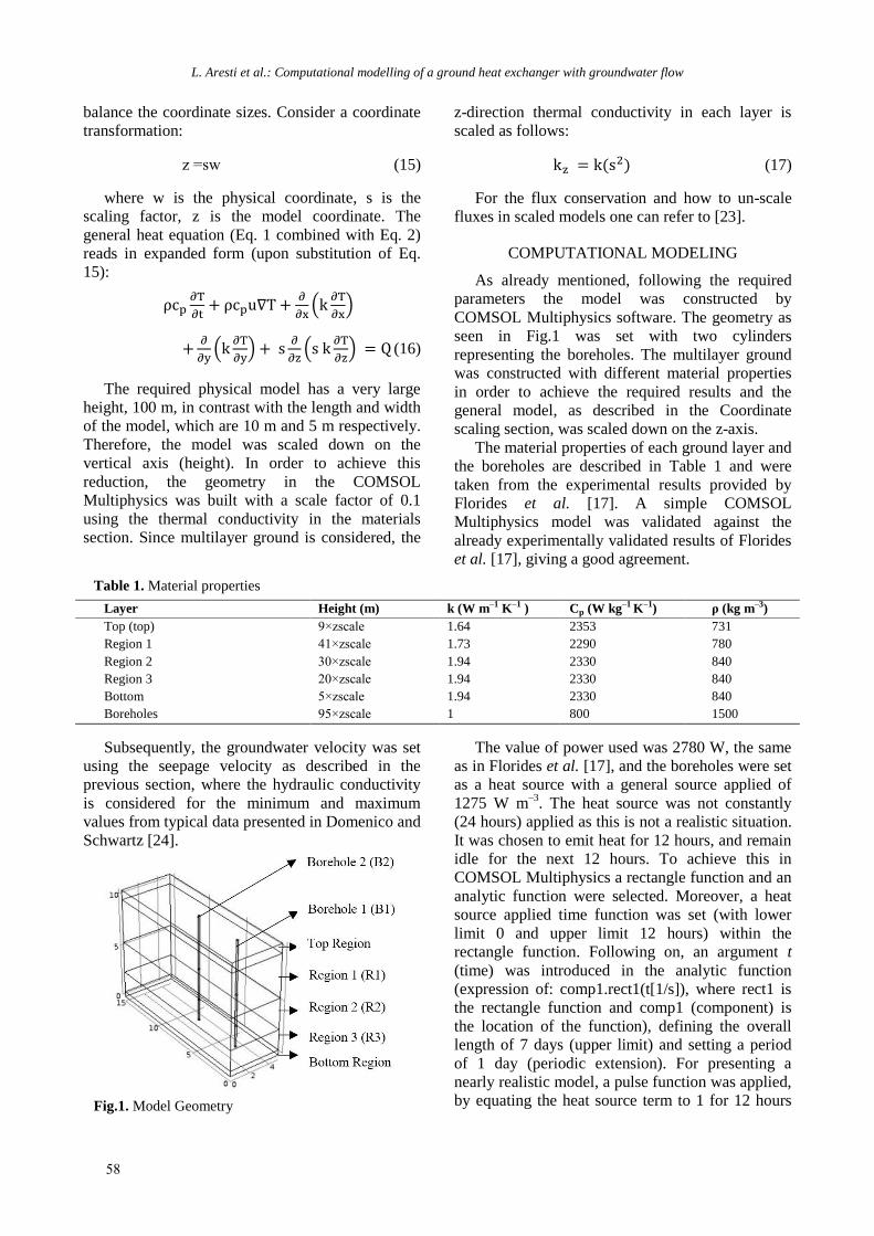
COMSOL Multiphysics software. The geometry as

seen in Fig.1 was set with two cylinders

representing the boreholes. The multilayer ground

was constructed with different material properties

in order to achieve the required results and the

general model, as described in the Coordinate

scaling section, was scaled down on the z-axis.

The material properties of each ground layer and

the boreholes are described in Table 1 and were

taken from the experimental results provided by

Florides et al. [17]. A simple COMSOL

Multiphysics model was validated against the

already experimentally validated results of Florides

et al. [17], giving a good agreement.

Table 1. Material properties

Layer Height (m) k (W m–1 K–1 ) Cp (W kg–1 K–1) ρ (kg m–3)

Top (top) 9×zscale 1.64 2353 731

Region 1 41×zscale 1.73 2290 780

Region 2 30×zscale 1.94 2330 840

Region 3 20×zscale 1.94 2330 840

Bottom 5×zscale 1.94 2330 840

Boreholes 95×zscale 1 800 1500

Subsequently, the groundwater velocity was set

using the seepage velocity as described in the

previous section, where the hydraulic conductivity

is considered for the minimum and maximum

values from typical data presented in Domenico and

Schwartz [24].

Fig.1. Model Geometry

The value of power used was 2780 W, the same

as in Florides et al. [17], and the boreholes were set

as a heat source with a general source applied of

1275 W m–3

. The heat source was not constantly

(24 hours) applied as this is not a realistic situation.

It was chosen to emit heat for 12 hours, and remain

idle for the next 12 hours. To achieve this in

COMSOL Multiphysics a rectangle function and an

analytic function were selected. Moreover, a heat

source applied time function was set (with lower

limit 0 and upper limit 12 hours) within the

rectangle function. Following on, an argument t

(time) was introduced in the analytic function

(expression of: comp1.rect1(t[1/s]), where rect1 is

the rectangle function and comp1 (component) is

the location of the function), defining the overall

length of 7 days (upper limit) and setting a period

of 1 day (periodic extension). For presenting a

nearly realistic model, a pulse function was applied,

by equating the heat source term to 1 for 12 hours

58


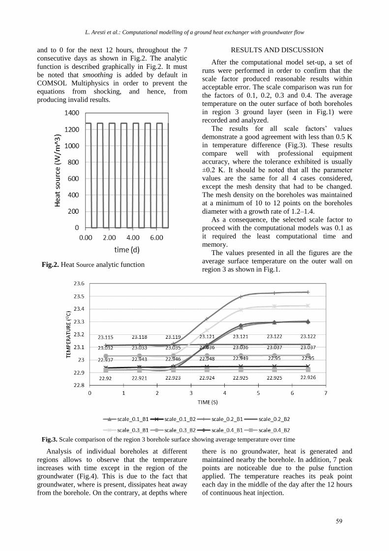
and to 0 for the next 12 hours, throughout the 7

consecutive days as shown in Fig.2. The analytic

function is described graphically in Fig.2. It must

be noted that smoothing is added by default in

COMSOL Multiphysics in order to prevent the

equations from shocking, and hence, from

producing invalid results.

Fig.2. Heat Source analytic function

RESULTS AND DISCUSSION

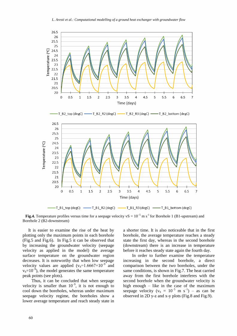
After the computational model set-up, a set of

runs were performed in order to confirm that the

scale factor produced reasonable results within

acceptable error. The scale comparison was run for

the factors of 0.1, 0.2, 0.3 and 0.4. The average

temperature on the outer surface of both boreholes

in region 3 ground layer (seen in Fig.1) were

recorded and analyzed.

he results for all scale factors’ values

demonstrate a good agreement with less than 0.5 K

in temperature difference (Fig.3). These results

compare well with professional equipment

accuracy, where the tolerance exhibited is usually

±0 2 It should be noted that all the parameter

values are the same for all 4 cases considered,

except the mesh density that had to be changed.

The mesh density on the boreholes was maintained

at a minimum of 10 to 12 points on the boreholes

diameter with a growth rate of 1.2–1.4.

As a consequence, the selected scale factor to

proceed with the computational models was 0.1 as

it required the least computational time and

memory.

The values presented in all the figures are the

average surface temperature on the outer wall on

region 3 as shown in Fig.1.

Fig.3. Scale comparison of the region 3 borehole surface showing average temperature over time

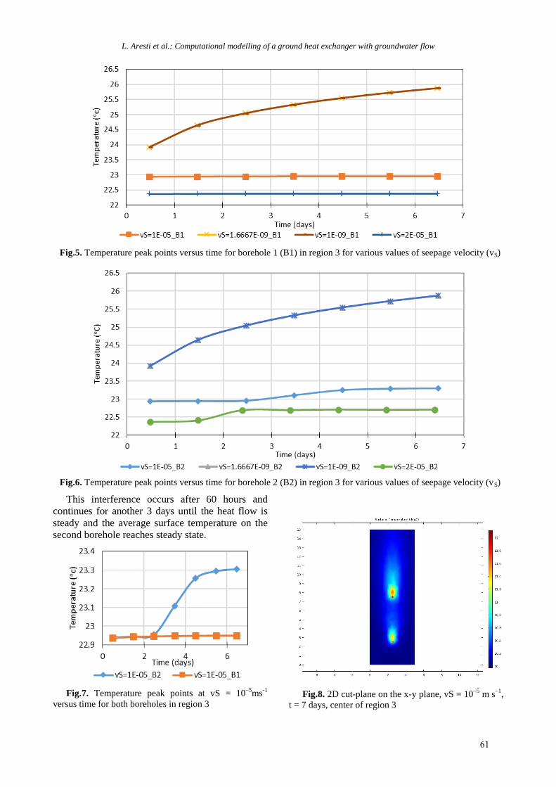
Analysis of individual boreholes at different

regions allows to observe that the temperature

increases with time except in the region of the

groundwater (Fig.4). This is due to the fact that

groundwater, where is present, dissipates heat away

from the borehole. On the contrary, at depths where

there is no groundwater, heat is generated and

maintained nearby the borehole. In addition, 7 peak

points are noticeable due to the pulse function

applied. The temperature reaches its peak point

each day in the middle of the day after the 12 hours

of continuous heat injection.

59


Fig.4. Temperature profiles versus time for a seepage velocity vS = 10

–5 m s

-1 for Borehole 1 (B1-upstream) and

Borehole 2 (B2-downstream)

It is easier to examine the rise of the heat by

plotting only the maximum points in each borehole

(Fig.5 and Fig.6). In Fig.5 it can be observed that

by increasing the groundwater velocity (seepage

velocity as applied in the model) the average

surface temperature on the groundwater region

decreases. It is noteworthy that when low seepage

velocity values are applied (vS 1 6667×10–9

and

vS=10–9

), the model generates the same temperature

peak points (see plots).

Thus, it can be concluded that when seepage

velocity is smaller than 10–9

, it is not enough to

cool down the boreholes, whereas under maximum

seepage velocity regime, the boreholes show a

lower average temperature and reach steady state in

a shorter time. It is also noticeable that in the first

borehole, the average temperature reaches a steady

state the first day, whereas in the second borehole

(downstream) there is an increase in temperature

before it reaches steady state again the fourth day.

In order to further examine the temperature

increasing in the second borehole, a direct

comparison between the two boreholes, under the

same conditions, is shown in Fig.7. The heat carried

away from the first borehole interferes with the

second borehole when the groundwater velocity is

high enough – like in the case of the maximum

seepage velocity (vS = 10–5

m s–1

) – as can be

observed in 2D y-z and x-y plots (Fig.8 and Fig.9).

60


Fig.5. Temperature peak points versus time for borehole 1 (B1) in region 3 for various values of seepage velocity (vS)

Fig.6. Temperature peak points versus time for borehole 2 (B2) in region 3 for various values of seepage velocity (vS)

This interference occurs after 60 hours and

continues for another 3 days until the heat flow is

steady and the average surface temperature on the

second borehole reaches steady state.

Fig.7. Temperature peak points at vS = 10

–5ms

-1

versus time for both boreholes in region 3

Fig.8. 2D cut-plane on the x-y plane, vS = 10–5

m s–1

,

t = 7 days, center of region 3

61


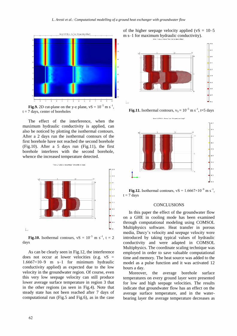
Fig.9. 2D cut-plane on the y-z plane, vS = 10–5

m s–1

,

t = 7 days, center of boreholes

The effect of the interference, when the

maximum hydraulic conductivity is applied, can

also be noticed by plotting the isothermal contours.

After a 2 days run the isothermal contours of the

first borehole have not reached the second borehole

(Fig.10). After a 5 days run (Fig.11), the first

borehole interferes with the second borehole,

whence the increased temperature detected.

Fig.10. Isothermal contours, vS = 10–5

m s–1

, t = 2

days

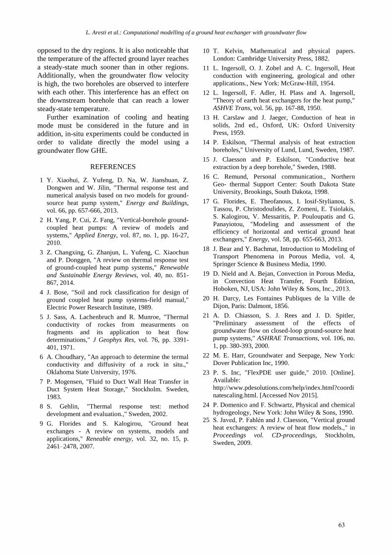
As can be clearly seen in Fig.12, the interference

does not occur at lower velocities (e.g. vS =

1 6667×10–9 m s–1 for minimum hydraulic

conductivity applied) as expected due to the low

velocity in the groundwater region. Of course, even

this very low seepage velocity can still produce

lower average surface temperature in region 3 that

in the other regions (as seen in Fig.4). Note that

steady state has not been reached after 7 days of

computational run (Fig.5 and Fig.6), as in the case

of the higher seepage velocity applied (vS = 10–5

m s–1 for maximum hydraulic conductivity).

Fig.11. Isothermal contours, vS = 10–5

m s–1

, t=5 days

Fig.12. Isothermal contours, vS 1 6667×10–9

m s–1

,

t = 7 days

CONCLUSIONS

In this paper the effect of the groundwater flow

on a GHE in cooling mode has been examined

through computational modeling using COMSOL

Multiphysics software. Heat transfer in porous

media, Darcy’s velocity and seepage velocity were

introduced by taking typical values of hydraulic

conductivity and were adapted in COMSOL

Multiphysics. The coordinate scaling technique was

employed in order to save valuable computational

time and memory. The heat source was added to the

model as a pulse function and it was activated 12

hours a day.

Moreover, the average borehole surface

temperatures on every ground layer were presented

for low and high seepage velocities. The results

indicate that groundwater flow has an effect on the

average surface temperature, and in the water-

bearing layer the average temperature decreases as

62


opposed to the dry regions. It is also noticeable that

the temperature of the affected ground layer reaches

a steady-state much sooner than in other regions.

Additionally, when the groundwater flow velocity

is high, the two boreholes are observed to interfere

with each other. This interference has an effect on

the downstream borehole that can reach a lower

steady-state temperature.

Further examination of cooling and heating

mode must be considered in the future and in

addition, in-situ experiments could be conducted in

order to validate directly the model using a

groundwater flow GHE.

REFERENCES

1 Y. Xiaohui, Z. Yufeng, D. Na, W. Jianshuan, Z.

Dongwen and W. Jilin, "Thermal response test and

numerical analysis based on two models for ground-

source heat pump system," Energy and Buildings,

vol. 66, pp. 657-666, 2013.

2 H. Yang, P. Cui, Z. Fang, "Vertical-borehole ground-

coupled heat pumps: A review of models and

systems," Applied Energy, vol. 87, no. 1, pp. 16-27,

2010.

3 Z. Changxing, G. Zhanjun, L. Yufeng, C. Xiaochun

and P. Donggen, "A review on thermal response test

of ground-coupled heat pump systems," Renewable

and Sustainable Energy Reviews, vol. 40, no. 851-

867, 2014.

4 J. Bose, "Soil and rock classification for design of

ground coupled heat pump systems-field manual,"

Electric Power Research Institute, 1989.

5 J. Sass, A. Lachenbruch and R. Munroe, "Thermal

conductivity of rockes from measurments on

fragments and its application to heat flow

determinations," J Geophys Res, vol. 76, pp. 3391-

401, 1971.

6 A. Choudhary, "An approach to determine the termal

conductivity and diffusivity of a rock in situ.,"

Oklahoma State University, 1976.

7 P. Mogensen, "Fluid to Duct Wall Heat Transfer in

Duct System Heat Storage," Stockholm. Sweden,

1983.

8 S. Gehlin, "Thermal response test: method

development and evaluation.," Sweden, 2002.

9 G. Florides and S. Kalogirou, "Ground heat

exchanges - A review on systems, models and

applications," Reneable energy, vol. 32, no. 15, p.

2461–2478, 2007.

10 T. Kelvin, Mathematical and physical papers.

London: Cambridge University Press, 1882.

11 L. Ingersoll, O. J. Zobel and A. C. Ingersoll, Heat

conduction with engineering, geological and other

applications., New York: McGraw-Hill, 1954.

12 L. Ingersoll, F. Adler, H. Plass and A. Ingersoll,

"Theory of earth heat exchangers for the heat pump,"

ASHVE Trans, vol. 56, pp. 167-88, 1950.

13 H. Carslaw and J. Jaeger, Conduction of heat in

solids, 2nd ed., Oxford, UK: Oxford University

Press, 1959.

14 P. Eskilson, "Thermal analysis of heat extraction

boreholes," University of Lund, Lund, Sweden, 1987.

15 J. Claesson and P. Eskilson, "Conductive heat

extraction by a deep borehole," Sweden, 1988.

16 C. Remund, Personal communication., Northern

Geo- thermal Support Center: South Dakota State

University, Brookings, South Dakota, 1998.

17 G. Florides, E. Theofanous, I. Iosif-Stylianou, S.

Tassou, P. Christodoulides, Z. Zomeni, E. Tsiolakis,

S. Kalogirou, V. Messaritis, P. Pouloupatis and G.

Panayiotou, "Modeling and assessment of the

efficiency of horizontal and vertical ground heat

exchangers," Energy, vol. 58, pp. 655-663, 2013.

18 J. Bear and Y. Bachmat, Introduction to Modeling of

Transport Phenomena in Porous Media, vol. 4,

Springer Science & Business Media, 1990.

19 D. Nield and A. Bejan, Convection in Porous Media,

in Convection Heat Transfer, Fourth Edition,

Hoboken, NJ, USA: John Wiley & Sons, Inc., 2013.

20 H. Darcy, Les Fontaines Publiques de la Ville de

Dijon, Paris: Dalmont, 1856.

21 A. D. Chiasson, S. J. Rees and J. D. Spitler,

"Preliminary assessment of the effects of

groundwater flow on closed-loop ground-source heat

pump systems," ASHRAE Transactions, vol. 106, no.

1, pp. 380-393, 2000.

22 M. E. Harr, Groundwater and Seepage, New York:

Dover Publication Inc, 1990.

23 P. S. Inc, "FlexPDE user guide," 2010. [Online].

Available:

http://www.pdesolutions.com/help/index.html?coordi

natescaling.html. [Accessed Nov 2015].

24 P. Domenico and F. Schwartz, Physical and chemical

hydrogeology, New York: John Wiley & Sons, 1990.

25 S Javed, Fahlén and J Claesson, "Vertical ground

heat exchangers: A review of heat flow models.," in

Proceedings vol. CD-proceedings, Stockholm,

Sweden, 2009.

63

Computational modelling of a ground heat exchanger with...

Documents

Transcript of Computational modelling of a ground heat exchanger with...