Computational modeling of ultrasound propagation using ...

2013 Simulia UK Regional User Meeting

1

Computational modeling of ultrasound propagation using

Abaqus explicit

Alison J. McMillan

Glyndwr University



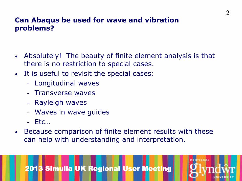
2 Can Abaqus be used for wave and vibration problems?

• Absolutely! The beauty of finite element analysis is that there is no restriction to special cases.

• It is useful to revisit the special cases:

- Longitudinal waves

- Transverse waves

- Rayleigh waves

- Waves in wave guides

- Etc…

• Because comparison of finite element results with these can help with understanding and interpretation.


3

Ultra-sound as a method for Non Destructive Testing

• Ultra-sound is an acoustic wave with frequency above the range of human hearing, about 20,000 Hz.

• For the NDT of engineering materials, the useful range is 2 – 10×106 Hz, although for some lower density materials, the range 50 – 500×103 Hz is also used.

• Ultrasound NDT can be used to detect the presence of sub-surface defects and thickness profiles of features.


4

Waves in solids

Phase velocity of waves:

• Longitudinal

𝑐𝐿 =𝐸(1 − 𝜈)

𝜌(1 + 𝜈)(1 − 2𝜈)

• Transverse

𝑐𝑇 =𝐸

2𝜌(1 + 𝜈)

• Where a plane wave front impinges on a boundary, then typically both a longitudinal and transverse reflection and transmission will take place.


5

Waves in solids

Rayleigh waves

• Phase velocity

𝑐𝑅 = 𝑐𝑇0.862 + 1.14𝜈

1 + 𝜈

• This wave travels along the free surface, with motion perpendicular to the surface.

Hopkinson’s bar – 1D wave guide:

• Used for measuring the stress-strain properties of materials at high strain rate

𝑐𝐵 = 𝐸𝜌


6

Illustration – waves and vibrations in a beam

Flexural waves in a Bernoulli-Euler beam

• The governing equation

𝐸𝐼𝜕4𝑈3𝜕𝑥4

+ 𝜌𝐴𝜕2𝑈3𝜕𝑡2

= 𝑞(𝑥, 𝑡)

• Flexural rigidity, 𝐼 = 𝑤ℎ3 12

• Cross-sectional area, 𝐴 = 𝑤ℎ

• Time dependent forcing term, 𝑞 𝑥, 𝑡

• Phase velocity is dispersive (velocity depends on wavelength)

𝑐𝐹 =2𝜋

𝜆

𝐸𝐼

𝜌𝐴


7

Standing waves: Modal analysis

• Natural vibration modes are solutions of

𝐸𝐼𝜕4𝑈3𝜕𝑥4

+ 𝜌𝐴𝜕2𝑈3𝜕𝑡2

= 0

with boundary conditions encastre at one end and free at the other:

𝑈3 𝑥, 𝑡 = 𝑎𝑘𝑔𝑘 𝑥 sin(𝛼𝑘𝑘 𝑡)

𝑔𝑘 𝑥 = 𝐶𝑘 sin 𝑝𝑘𝑥 − sinh 𝑝𝑘𝑥 + 𝑅𝑘 cos 𝑝𝑘𝑥 − cosh 𝑝𝑘𝑥

𝑝𝑘 are the roots of cos 𝑝𝑘𝐿 + 1 cosh 𝑝𝑘𝐿 = 0

with 𝛼𝑘 = 𝐸𝐼 𝜌𝐴 (𝑝𝑘𝐿)2 and 𝑎𝑘 = 𝑔𝑘(𝐿) (𝜌𝐴𝛼𝑘)


8

Data used in this exercise

Aluminium properties

• Young’s modulus 70×103 MPa

• Poisson’s ratio 0.35

• Density 2.7×10-9 Tonnes/mm3

Beam geometry

• Length 100 mm

• Width 10 mm

• Thickness 2 mm

FEA model information

• Element type C3D8R, with

• Model comprising 40 by 10 by 10 elements


9

Modal analysis solutions

165 Hz

1032 Hz

2885 Hz


10

Low frequency forced motion

Quasi-static

• Applied forcing frequency << lower than the fundamental natural frequency

• The disturbance is transmitted through the component far quicker than the forced movement at the loading point

• Analysis run time is slow in Explicit analysis: more computationally efficient and no less rigorous to use an implicit analysis step


11

Intermediate frequency forced motion

• Selected forcing frequency 𝜔 = 50×103 rad/second

• This lies between the 4th and 5th flap modes

• At this frequency, 𝑐𝐹 =0.3834×106 mm/second and 𝜆𝐹 =48.18 mm

• Flexural wave takes 260.8×10-6 seconds to travel the length of the beam, 100 mm, cf the longitudinal and transverse waves, 15.50 and 32.27×10-6 seconds respectively

Deflection at measurement point

Time ×10-3 second 4 6 2 8 10 0


12

Wave pulse illustrated at 10×10-6 second intervals

Peak to peak 45-50 mm ≈ 𝜆𝐹

Wave travel distance ≈ 23 mm

10

50

20

30

40

60

300 ×10-6 seconds


13

Illustration of ultra-sound NDT of a 3D block

• Dimensions 20x20x10 mm

• Hole diameter 2 mm.

• Forcing frequency 5×106 Hz.


14

Surface deformation at 1×10-6 second intervals


15

Wave profile

0 – 0.3×10-6 seconds

1.8 – 2.1×10-6 seconds

4.7 – 5.0×10-6 seconds


16

Signals received at measurement points

1

2

3

4 time

1 2 3 4 ×10-6 second

Wave arrival times: Longitudinal Rayleigh

Mea

sure

men

t poi

nts


17

Conclusions and recommendations

• Abaqus explicit can be effective in simulating wave pulses in components

• The post-processing of results requires interpretation; the development of post-processing add-on tools is an area for further development

• Abaqus explicit modelling can provide simulated data for demonstrating data processing techniques that could then be used on NDT data

• Simulated NDT data for components containing defects could then be used as reference catalogues, improving the interpretation capability of NDT

Computational modeling of ultrasound propagation using ...

Documents

Transcript of Computational modeling of ultrasound propagation using ...