Computational Methods for Structural

Bioinforamtics

and Computational Biology (4)

(Protein structure and Monte Carlo sampling)

Jie Liang 梁 杰

Molecular and Systems Computational Bioengineering Lab (MoSCoBL)Department of Bioengineering

University of Illinois at Chicago上海交通大学系统医学研究院

上海生物信息技术研究中心

E-mail: jliang@uic.eduwww.uic.edu/~jliang

Dragon Star Short CourseSuzhou University, June 14 – June 18, 2009

Today’s Lecture

Simplified structural models

Markov chain Monte Carlo: Generating conformational samples

Bayesian estimator of molecular evolution

Sequential Monte Carlo:Generating conformational samples

Generating Molecular Conformations: Folding and Growth

Folding Method: Markov chain Monte Carlo

Growth Method: Sequential Importance Sampling

Simplified Models: Sequence and Structure

ACDEFGHIKL….

Sequences Structures

ACDLW

HP

A

Off-lattice

3D-Lattice

2D

Functions

Why simplified models?

Simplified structural model leads to drastically reduced conformational space

Enable enumeration or very thorough sampling

Can help to reveal most important principles

Simplified Model. 2D Lattice Model

ACDEFGHIKL….

Sequence space Structure space

ACDLW

HP

A

Off-lattice

3D-Lattice

2D

2-D Lattice Model

Contacts

Contact number t

Compactness ρ

= t /tmax

Voids

Lattice model for folding study

Lattice 2D HP models: Enumerating sequences and conformations.

Exact thermodynamics.

Exact effects of sequence variation.

Folding dynamics:Exact folding dynamics.

(Cieplak

et al, 98; Banu

and Dill, 00)

(Lau and Dill, 1989)

(Sëma

Kachalo, Hsiao-Mei

Lu, and Jie

Liang, Phys Rev Lett, 2006, 96:

058105.1-4

)

HP Sequences and Conformations

A

B

C

D

E

F

G

H

I

J

K

L

M

N

O

P

Q

R

S

T

U

V

W

X

Y

Z

• Chain length: 16• 802,075 conformations, 216

sequences

• 1,539 HP sequences fold tounique ground states.

• 456 structural families– from 1 (low designability)– to 26 (high designability) sequences

0;0;1 =Δ=Δ−=Δ PPHPHH EEE

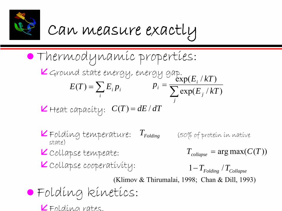
Can measure exactly

Thermodynamic properties: Ground state energy, energy gap.

Heat capacity:

Folding temperature: (50% of protein in native state)

Collapse tempeate:Collapse cooperativity:

Folding kinetics:Folding rates.

(Klimov

& Thirumalai, 1998; Chan & Dill, 1993)

dTdETC /)( =

FoldingT

CollapseFolding TT /1−

∑=i

ii pETE )( ∑=

jj

ii kTE

kTEp

)/exp()/exp(

))(max(arg TCTcollapse =

Simplified Model. Side Chain Models

ACDEFGHIKL….

Sequence space Structure space

ACDLW

HP

A

Off-lattice

3D-Lattice

2D

Side Chain Models

a b

Maximum Compact Conformation

Computation of Side Chain Entropy

3 5 7

2 4 6 8

p

2

3

4

5

6

7

8

1 9

a

b

Rotamer counting: 2187

Exact number: 21*55 = 1155

Structure with Maximum Side Chain Entropy

Chirality

i-1 i i+1

empty

Ssci

i

i+1i-1

R

emptysci

a b

Studies with Side Chain Models

Why residues are chiral?Chiral models have much lower folding entropy than achiral models.

Why different side chains?Models with less flexible side chains have lower folding entropy than models with more flexible side chains.

Protein packing:not like a jigsaw puzzle, but more like nuts and bolts in a jar.

Jinfeng

Zhang, Rong

Chen and Jie

Liang. Empirical potential function for simplified protein

models: Combining contact and local sequence-structure descriptors

Proteins, 2005, 63(4):949-960.

Entropy and Side Chain Entropy

Entropy S(ρ): S(ρ) = kB lnn(ρ),

Side chain entropy: Ssc (B) = kB lnnsc (B),

Overall entropy: Sall = kB ln∑n(ρi ) = kB ln∑nsc (Bi ),

Simplified Model. Off-lattice Models

ACDEFGHIKL….

Sequence space Structure space

ACDLW

HP

A

Off-lattice

3D-Lattice

2D

32-state Model

α

t+1

tt-1

o

1.5

o

1.5 A

60o

A

Sample Structures

Simplified Model. Off-lattice Protein Model

ACDEFGHIKL….

Sequence space Structure space

ACDLW

HP

A

Off-lattice

3D-Lattice

2D

Discrete State Model

αi

τiCi+1

Ci

Ci-1

Ci-2

SCi

SCi-1

Bond angle αI is determined by Ci-1 ,Ci , and Ci+1 ;Dihedral angle τi is determined by Ci-2 , Ci-1 , Ci , and Ci+1 ;

Cα

One approach is to parametrize

by two angles:

How to develop discrete state model?

80 100 120 140 160

−15

0−

100

−50

050

100

150

Bond and torsion angles for all AA

bond angle

tors

ion

angl

e

Ramachandran plots

Distribution of bond and torsion angles in real proteins

Clustering of Discrete Angles

K-means clustering

Angle values for the

K-states.80 100 120 140 160

−1

50

−5

00

50

10

0

Distribution of ALA

Bond angle

Dih

ed

ral a

ng

le

80 100 120 140 160

−1

50

−5

00

50

10

0

Distribution of GLY

Bond angle

Dih

ed

ral a

ng

le

80 100 120 140 160

−1

50

−5

00

50

10

0

Distribution of PRO

Bond angle

Dih

ed

ral a

ng

le

80 100 120 140 160

−1

50

−5

00

50

10

0

Distribution of HIS

Bond angle

Dih

ed

ral a

ng

le

How good are discrete state models?

<4 A: near natives

1-2 A: X-ray crystallographyresolution

(Zhang et al2005, Proteins)

Simplified Model for Sequence

20 amino acids can be simplified to seven letter alphabet as:(C); (I,V,L,M,W,F,Y); (E,K,A,Q,R); (G); (S,H,T); (P); (D,N).

CY

SIL

EV

AL LE

UM

ET TR

PP

HE

TY

RG

LULY

S ALA

GLN

AR

GG

LYS

ER

HIS

TH

RP

RO

AS

PA

SN

0.0

0.1

0.2

0.3

0.4

0.5

0.6

With discrete state, any protein structure can be represented by a sequence of (a,s).

First order state transition propensity

p[(ai

,si

),(ai+1

,si+1

)]

Today’s Lecture

Simplified structural models

Markov chain Monte Carlo:Bayesian estimation of model of molecular evolution

Sequential Monte Carlo: Generating conformational samples

Conformation Generation

Starting from an initial conformation

Make small changes, many times to transform it into a protein like conformation

Move set:To change conformations, often locally.

Energy function:To evaluate generated conformation.

Physical Move Set

Generalizedcorner moves

Generalizedcrankshaft moves

Single point(pivot) moves

Allowed moves are physically realizable

on 2D square lattice.

⎩⎨⎧

<≥

−→ji

kTEEji

ji EEeEE

rji ,,1

~ /)(Transition rate from Metropolis dynamics:

Generic Move Set

Cut a fragment of a conformation

Replace it with a fragment of another conformation when it fits.

Sampling from a Distribution

But that is not all!Need to calculate ensemble properties of proteins

Radius of gyrationRg

= ∫

|x1

– xN

|p(x

)dx,

where conformation x has its first and last residues at x1

and xN

, and p(x

)is the Boltzmann

probability

Free energy: F = -kt ln Z, where partition function Z = ∫

p(x

)dx,

Need to generate samples from the Boltzmanndistribution π(x) under an energy function E( x) for conformations { x }

General ProblemNeed to calculate

I = ∫D

f(x) π

(x) d xChallenge: x is high dimension, π (x) may be complicated

Can approximate withI’ = ∑i f(xi

)/mif we can generate m independent random samples from target distribution π

(x)

Law of large number: limm->∞ I’ = ICentral Limit Theorem: Error is in the order of O(m1/2), depending on variance of f(x) in region D

Sampling from a Distribution

How to sample from a distribution?It is easy to evaluate the probability π(x) of a conformation xif already generated

But not always possible to generate samples {x} directly from a distribution π(x)

Sampling from uniform distribution U[0, 1]

Implemented in most language

Sampling from the Gaussian distributionBox-Muller Transformation

Central limit theorem

Rejection Sampling

Goal: Sampling from a target distribution π(x) Sampling x from an easy distribution function g(x),

such that M g(x) > c π(x) always hold

Now, another random number r from U[0, 1]

Accept if r < M g(x)/c π(x)

Accepted samples {x} follow π(x) !Why does this work?

Problem: mostly rejecting samples in high dimensional space.

von Neumann

Another approach

Use a Markov chain:A sequence of random variables { x1, x2 …, xt}Xt+1 is obtained from a

transition rule / proposal function / trial distribution T(xt, Xt+1

) eg. by move set

Under mild conditions, a Markov chain reaches a unique stationary distribution π(.)

Aperiodic, irreducible, recurrentSamples will be CORRELATED samples from π(.)

Initial starting position unimportantRemove the first k number of samples: burning-in period.

Convergence speed (mixing rate)Depends on the second eigen value of the transition matrix

Design of a Markov chain

How to design a Markov chain such that its stationary distribution is the target distribution we want?

Surprisingly easy!

Key: construct a transition rule so the stationary distribution is invariant.

time-reversible Markov chain does it!Can you tell if a movie is played backward?

Can be obtained so long the detailed balance condition is satisfied

Detailed balance condition:π

(X) A(x , y )

= π

(y) A( y , x

)

Metropolis-Hastings Algorithm

Given current state Xt , draw y from proposal distribution T(xt , y )

eg. move set

Draw another random number u from U[0, 1], and update:

xt+1 = y, if u< r( xt+1, y)xt+1 = xt, otherwise

where r( xt+1, y)=min{1, π

(y)T(y , x )/ π

(x)T(x , y )}

Note: The actual transition rule is:

A(x , y )=

T

(x ,

y

)r(x , y )

Applications

Generating proper conformational samples from the Boltzmanndistribution of a given energy function

Other bioinformatics application:Study of molecular evolution

Evolutionary Model

Assuming no insertion and deletion

Relationship between proteins (species) can be described by a phylogenetic tree

Binary tree:

No multifurcation

Ignore horizontal transfer of genes

Residue substitution follows a Markovian process

A i ti v ibilit

20 × 20 rate matrix Q for the instantaneous substitution rates of 20 amino acid residues

,}{

2,201,20

20,21,2

20,12,1

⎟⎟⎟⎟⎟

⎠

⎞

⎜⎜⎜⎜⎜

⎝

⎛

−

−−

==

ΛΟΛΛ

qq

qqqq

qQ ij

• Transition probability matrix can be derived from Q :

matrix. diagonal : rs,eigenvectoleft :

rs,eigenvectoright :1

1 )0()exp()0()exp()}({)(

Λ

Λ===

−

−

U

U

PUtUPQttptP ij

Model: Continuous time Markov process for substitution

(Felsenstein, 1983; Yang 1994; Whelan and Goldman, 2000;

Tseng and Liang, 2004)

• Model parameters: Q

Likelihood function of a given phylogeny

• Given a set of multiple-aligned sequences S = (x1 , x2 , ..., xs ) and a phylogenetic tree T = ( V, E ),

A column xh at poisition h is represented as:

xh

= ( x1,h

, x2,h

, …, xs,h

)

• The Likelihood function of observing these sequences is:

∏

∑ ∏

=

∈ ∈

==

=

∈

s

hhs

xIi ji

ijxxxh

QTxpQTxxPQTSP

tpQTxp

Ai

jik

11

),(

),|(),|,(),|(

:sequence Whole

)(),|(

:column One

Λ

ε

π

1

10 11 12 13 14 15 16

2 3 4 5 6 7 8 9

0.1 substitution/site

Bayesian Model

• Posterior probability distribution of rate matrix given the sequences and tree:

on.distributiposterior :),|( on,distributi likelihood :),|(

on,distributiprior :)( where

,)( ),|(),|(

TSQQTSP

Q

dQQQTSPTSQ

π

π

ππ ∫ ⋅∝

• Bayesian estimation of posterior mean of rates in Q :

Eπ

(Q) = ∫

Q ·

π

(Q | S, T) d Q,

• Estimated by Markov chain Monte Carlo.

Markov chain Monte Carlo method for parameter estimation

Target distribution π : posterior probability function

Can evaluate this function π, but direct sampling from it is impossible!

Generate (correlated) samples from the target distribution π

Run a Markov chain with π as its stationary distribution

Markov chain Monte Carlo

• Proposal function:),,(),(),( 1111 ++++ ⋅== ttttttt QQrQQTQQAQ

• Detailed balance: samples target distribution after convergency.

• Metropolis-Hastings Algorithm:

),,(),|(),(),|( 111 tttttt QQATSQQQATSQ +++ ⋅=⋅ ππ

]1,0[ fromnumber random a is where

},),(),|(),(),|(,1min{),(

1

111

UuQQTTSQ

QQTTSQQQruttt

ttttt

+

+++ ⋅

⋅=≤

ππ

• Collect data from m acceptant samples

Eπ

(Q) ≈∑i=1m

Qi / m ≈

∫

Q ·

π

(Q | S, T ) d Q.

Move Set

• Two types of moves : s1

, s2

⎟⎟⎠

⎞⎜⎜⎝

⎛=⎟⎟

⎠

⎞⎜⎜⎝

⎛1.09.01.09.0

2,21,2

2,11,1

SSSS

• Block moves: s2

• Acceptance ratio:

Individual moves : 50%-66%

Block moves: <10%

.1.1 ,1.0 where

,

,

21

1,21,

1,11,

==

=

=

++

++

αα

α

α

tijtij

tijtij

qq

qq

1.1 ,1.0 where move, individual assimilarly moveblock within entries All

. },,{},,{},,,,,,{ },,{ },{

:]5,4,3,2,1[ from draw blocks residuedifferent 5

21 == αα

HRKEDQNMCTSWYFPG,A,V,L,I,

U

• Individual moves : s1

• Transition matrix between twotypes of moves:

Validation by simulation

Generate 16 artificial sequences from a known tree and known rates (JTT model)

Carboxypeptidase A2 precursor as ancestor, length = 147

Goal: recovering the substitution rates

1

10 11 12 13 14 15 16

2 3 4 5 6 7 8 9

0.1 substitution/site

Phylogenetic treeused to generate 16 sequences

1400

014

500

1500

015

500

0e+00 3e + 5 6e + 5

−log

likeh

ood

(−l)

Number of Steps14

057.0

1405

8.0

500000 504000 508000

(a)

Convergence of the Markov chain

Qauntifying estimation error

Relative contribution:

Weighted error in contribution:

Weighted mean square error (MSE ):

(Mayrose et al, 2004, Mol Biol Evo)

Accurate Estimation with > 20 residues and random initial values

75 0 100 200 300 4000.

001

0.00

30.

005

0.00

7Sequence Length

MSE

p

(d)

Accurate when > 20 residues in length.

Distribution of MSE of estimated rates starting from 50 sets of random initial values.

All MSE < 0.00075.

0.00045 0.00060 0.00075

05

1015

2025

30

MSEp

Freq

uenc

y

(c)

MS

E

(

A R N D C Q E G H I L K M F P S T W Y V

A

R

N

D

C

Q

E

G

H

I

L

K

M

F

P

S

T

W

Y

V

The Active Pocket [ValidPairs: 39]

(a)

A R N D C Q E G H I L K M F P S T W Y V

A

R

N

D

C

Q

E

G

H

I

L

K

M

F

P

S

T

W

Y

V

The rest of Surface [ValidPairs: 177]

(b)

A R N D C Q E G H I L K M F P S T W Y V

A

R

N

D

C

Q

E

G

H

I

L

K

M

F

P

S

T

W

Y

V

Interior [ValidPairs: 190]

(c)

A R N D C Q E G H I L K M F P S T W Y V

A

R

N

D

C

Q

E

G

H

I

L

K

M

F

P

S

T

W

Y

V

Surface [ValidPairs: 187]

(d)

Evolutionary rates of binding sites and other regions are different

Residues on protein functional surface experience different selection pressure.

Estimated substitution rate matrices of amylase:

•

Functional surface residues.

•

The remaining surface, •

The interior residues

•

All surface residues.

Sij (i, j) are residues shown in the same column of MSAdefined as Sampled Pairs and Sij are estimated by Baysian MCMC }

Today’s Lecture

Simplified structural models

Markov chain Monte Carlo:Bayesian estimation of model of molecular evolution

Sequential Monte Carlo: Generating conformational samples

Packing analysis

(Protein transition state ensemble}

^ �� � � \ � � �� �� a{z � �� cJ| }� �� � �� ~ ��� a � � } ~ � � � ^ �� � � \ �

i � 6& 0 - 9 ' o & 6 <. ' / ' 0 1 o ' 9p

i : ) - / r . ' 6 t ) 6& < - . 1 - '. /& ' 6h

z :; )& * <1 * * ' < /& 5 & / 7p

z v� < 9 r o 'o 51 9 r 0 'p

i v ) 6& '.2 1 . 6 ) 0 - 9 & * +p

i � ' 6 / t ) 6& < - . & * <& - 9 ' 612 - . 1 / '& * 2 1 9 o & * +p�

� �� � a � � ^ �� � � \ � � ` �� � � � � � �

i j ) . / 12 <1 0 - 9 ' 0 '* / 6 - ) < '2 r 9 9 7 <1 * / )& * 'o k & /; & * -1 9 7 0 '.� p

� f �� � � �� � � YO� � � � � � ��

i : )* 1 < < r . k ; '* � �� p

a b

i : )* t ' o ' / ' < / 'o t 7 ) 6& 0 - 9 ' t . ' ) o /; � . 6 / 6 ' ). <; ) 9 +1 . & /; 0 p

�

�` � � � ` �� � a z � � � � � �� � � �

i :1 *2 1 . 0 ) /& 1 * ) 9 6 - ) < 'p

i x '1 0 ' /. & < - . 1 - '. /& ' 6p

i j ) <n & * + o '* 6& / 7 ) * o <1 0 - ) < /* ' 6 6p�

� ) t 9 '� h :1 *2 1 . 0 ) /& 1 * ) 9 6 - ) < ' 12 ) �l -1 9 7 0 '. k & /; 51 & o 6p� � � � � � � � � � � � � � � � � � � � �   � � � � ¡ � � �  � � � � � �¡ ¢ ¢ � � � �¢ �   �   � � � �£   £   £ � � � �¤ ¥¦ ¥ ¦ � � � �¦ � ¤ � � ¤ � � � � �¥ ¤ ¡ � ¤   ¡ £ � � �� � � �   ¡ � ¥ ¥   ¡ � � � �� � ¢ ¢ �   ¢   ¥   � � � � � �� � � ¢ �   ¤ � ¡ ¢ � ¦ ¢ � ¥ � � ��   ¡ � £ � ¤   ¥ � ¤¦ � ¢   £   � �� ¡ � � � �¦ ¦ � � ¡ ¢ £ £ ¢ £ � � � � � �� ¢ � ¥ £ ¦ � £ �¦ � ¢ ¥ ¥ � £ � ¦ ¦ � � ¥ � �� £ ¦ � � � ¤ ¢ ¤ ¡ ¦     ¢ ¢   � ¡ ¥ ¢ ¥ � � �� ¤ � � ¢ ¢ £ £ ¤ � � � � � £ � � ¢ � � ¢ � �   ¢   � ��¦ ¢¦ �¦     ¢ ¢   � ¤¦ ¦ ¦ ¡ ¤ �   ¦ £ � � � ¢ � � � �� ¥ � ¢ ¢¦ �   ¡ � � ¡ � � �   ¦ ¥ �   � ¢ ¢ ¥ �   ¡ �¦ ¤ ¤ £ �� � ¡ �¦ ¦ ¥ ¢ ¤¦   ¤ ¤¦ ¡ ¡ ¡ ¤   ¥ ¤     £ � �   � � ¥ ¦ ¡ ¤ � �� � � � � � � � � ¡ £ � � � £ ¤   ¤ ¤ � � � � � ¥ ¡ ¢ £ ¡ � £ �   ¥ � £ ¦ � �� �   � � � � � ¤ ¢ ¡ � £ ¤ �   £ ¤ � �   � ¡ ¤ ¥ ¦ ¤ � � ¡ ¤ �¦ ¤ ¡ � � � ¥   £�   ¦ � ¢ ¢ ¤ � � £ � ¤ � � £ ¤   ¦ � £ ¥ �   £ �¦ ¤¦ ¡ ¡ ¤ ¥   ¢ ¢ ¢ ¡ ¥ ¥ ¦ � ¡� ¡ � � ¢¦   � £ ¤ � ¤ �¦ ¦   ¥ £ � � ¤ � � ¢ ¥ � ¥ ¢ ¤ ¤ ¡ � ¡ ¥ ¡ £ ¥ � � � �   ¡ ¢¦ ¡ � ¡� ¢ ¢ ¤ £ ¦ � ¥ ¥ £ £ ¢ ¢ � � ¢ ¢ ¥ � ¢ � � ¤ � ¤ ¢ � ¢¦ ¥ � ¡ ¡     ¤  ¦ � ¦ £ � ¤ ¡ ¦ � �   �

§l �

� �� �� � \ � ¨ � � � � a

i j . 1 t ) t & 9 & / 7 1 2 51 & o 2 1 . 0 ) /& 1 * h

© ª � �«¬ Y­ � ® � ¯ °­ ® � ¯

i v� - ' < / 'o * r 0 t '. 12 51 & o 6 <1 * / )& * 'o & * ) -1 9 7 0 '. h

±� ª � �«¬ Y­ � ® � ¯³² ´ °­ ® � ¯

i v� - ' < / 'o 51 & o 6&µ ' h±¶ � ª ­ ª ® � ¯³² ¶

­ ® � ¯

i v� - ' < / 'o k ) 9 9 6&µ ' 12 51 & o 6h±· ® � ¯ �

ª · ² ­ ª ¸º¹ ® � ¯­ ª ® � ¯

»

8 10 14 18 22

0.02

0.06

0.10

N

Voi

d P

roba

bilit

ya

10 15 20

0.02

0.06

0.10

N

Exp

ct N

um o

f Voi

ds b

10 15 200.00

0.10

0.20

N

Exp

ct V

oid

Siz

e

c

10 15 20

0.2

0.6

1.0

N

Exp

ct W

all S

ize

d

g & + r . '� h ¼½¾ ¿ ½À ÁÂ Ã Ä Á¾ Ľ ÁÀ ½Š¾ Æ ÃÇ È ÂÉ Ä¾ Ê Ë ¿ ½ ÁÅ Ì

Í

�\ � � � � � � � a� � � � �� \ �� ¨ �\ � � � a a

i j ) <n & * + o '* 6& / 7 h

Î � �� Ï ¶

k ; '. ' ) �l 0 '. ; ) 6 51 & o 612 ¶ 6& µ 'p

i :1 0 - ) < /* ' 6 6 h

Ð � ÑÑ ÒÓÔ

k ; '. ' Ñ & 6 /; ' * r 0 t '. 12 * 1 * t1 r * o 'o <1 * / ) < / 6p

Õ

10 15 200.99

00.

994

0.99

8

N

Exp

ecte

d P

acki

ng D

ensi

ty a

0.6 0.7 0.8 0.91e+

011e

+05

Packing Density

Num

ber

of C

onfo

rmat

ions

1−Void2−Voids3−Voids

b

5 10 15 20

0.10

0.20

0.30

N

Exp

ct C

ompa

ctne

ss

c

0.0 0.2 0.4 0.6 0.8 1.0

0.98

50.

990

0.99

51.

000

Compactness

Exp

ecte

d P

acki

ng D

ensi

ty

N = 22N = 20N = 18N = 16N = 14

d

g & + r . 'Ö h× È ÃØ Â É Ù�Ú ½ ÉÅ ÂÀ Ë Û Î Ü ÈÉ Ú Ã¾ ¿ Ä È ÃÀ É ½ Å Å Û Ð Ü È Á½ Ú ÂÝ ½ Á½ ÉÀ Ì

Y �

^ � � � � ` �� � a � �� � � �

i Þ 1 . ' & * / '. ' 6 /& * + t r / & 0 -1 6 6& t 9 ' /1 '* r 0 '. ) / 'p

i Þ 1 * / ' : ). 91 � - - . 1 ) <; h + '* '. ) / ' . )* o 1 0 6 ) 0 - 9 ' 6 /1 0 ) n '

& *2 '. '* < ' 61 * n ' 7 - ) . ) 0 ' / '. 6p

i Þ : Þ : 0 ' /; 1 o h 6 / ). /& * + k & /; )2 r 9 9 7 '� / '* o 'o <; )& * á '* +& * ' '.

) 6 ' â r '* < ' 1 2 . )* o 1 0 2 1 9 o & * + ã r *2 1 9 o & * + ® Þ ). n 1 5 ¯ 0 1 5 ' 6p

i x . 1 k /; 0 ' /; 1 o h + . 1 k & * + ) <; )& * -1 9 7 0 '. 1 * ' -1 9 7 0 '. ) / )

/& 0 ' r * /& 9 /; ' o ' 6& . 'o 9 '* + /; & 6 . ' ) <; 'op

z ä ' â r & . ' 0 '* / h 6 ' 92 l ) 51 & o & * +p

i ä ' å ' < /& 1 * Þ ' /; 1 o h 6& 0 - 9 ' . )* o 1 0 + . 1 k /; k & /; . ' å ' < /& 1 * 12 ) 9 9

<; )& * 6 /; ) / ). ' * 1 / 6 ' 92 l ) 51 & op

z æ r < < ' 6 6 . ) / ' & 6 /1 1 91 k 2 1 . 91 * + <; )& * 6p

Y f

ç r . ) - - . 1 ) <; h æ ' â r '* /& ) 9 Þ 1 * / ' : ). 91 ® æ ' â r '* /& ) 9 80 -1 . / )* < '

æ ) 0 - 9 & * + ¯ ®( & r è :; '* � é é� ¯

i � ). + ' / , & 6 /. & t r /& 1 * h 4 * &2 1 . 0 o & 6 /. & t r /& 1 * ) 0 1 * + ) 9 9 -1 6 6& t 9 '

æ � ê 612 9 '* + /; �p

i ä1 6 '* t 9 r /; 0 ' /; 1 o ® ä 1 6 '* t 9 r /; è ä1 6 '* t 9 r /; � éë ë ¯h * '� /

-1 9 7 0 '. / ) n ' 61 * ' 1 2 /; '� �\ � �� * '& +; t1 . & * + 6& / ' 6k & /; ' â r ) 9

- . 1 t ) t & 9 & / 7

z 3 & ) 6 'o 6 ) 0 - 9 & * +p

z q ' 'o /1 t 'k '& +; / 'op

Y y

ä1 6 '* t 9 r /; Þ ' /; 1 o ho o

o

o o o

o oo

o ooo

o ooo

o oo o

o o oo

o o o o

o o oo

o ooo

o ooo

o oo o

o oooo

o ooo

o

o oooo

o oooo

o ooo o

o oo o

o

o oo o o

o oo o

o

o o ooo

o o ooo

o o oo o

o o o oo

o o o o o o o o oo

o o ooo

o o ooo

o o oo o

o oooo

o ooo

o

o oooo

o oooo

o ooo o

o oo o

o o oo o o

o oo o

o

1/3

1/3*1/3

1/3*1/3 = 1/27 < 1/25

1/3*1/3*1/2 = 1/18 > 1/25

1/3*/1/3*1/3

Y �

�\ �� � � ìí îðï íñ òóô õö ÷ñ ò í øô ù õ ÷ ® � ¯

, . )k úüûý þY á ÿ � � �� � � � �2 . 1 0 � Y ® ú Y ¯

æ ' / /; ' & * <. ' 0 '* / ) 9 k '& +; / · ûý þY � © Y ® úûý þY ¯ ° � Y ® úûý þY ¯

� �� Ñ � � � � � � �

� �� ÿ � � � � �

� �� È ¿ Ä ÊÂ É Ù Æ¾ ÁÀ Ç ½ ® Ñ Ï � ¯�À Ç ¿¾ ɾ ¿ ½ Á ƾ ÁÀ Ç ½ ÿ À Ç Å È ¿ Ä Ê½

, . )k -1 6& /& 1 * úûý þ� Y2 . 1 0

� � Y ® ú � Y � úûý þY � � � úûý þ� ¯

� ��� ¾ ¿ Ä��À ½ À Ç ½ ÂÉ Ã Á½ ¿ ½ ÉÀ È Ê� ½  ٠ÇÀ Ì

� ûý þ� Y�� © � Y ® úûý þY � � � úûý þ� Y ¯

© � ® úûý þY � � � úûý þ� ¯² � � Y ® úûý þ� Y � úûý þY � � � úûý þ� ¯· ûý þ� Y � �ûý þ� Y ² · ûý þ�

�� � � ���½Å È ¿ Ä ÊÂ É Ù

�� � � ��

Y �

8*2 '. '* < ' 1 * )* 7 + '1 0 ' /. & < 1 . -; 7 6& < ) 9 - ). ) 0 ' / '. 6h

� � ���� ® ú Y �� � � � ú � ¯ "!Òý ¬ Y� ® úûý þY �� � � � úüûý þ� ¯ · ûý þ

Òý ¬ Y · ûý þ

v� ) 0 - 9 ' 6 h

i v * o l /1 l '* o o & 6 / )* < ' h � ® ú Y �� � � � ú � ¯ � � � ú � � ú Y � � f

i � 5 '. ) + ' 51 & o 6& µ ' h � ® ú Y �� � � � ú � ¯ � /1 / ) 9 51 & o 6& µ ' & *

® ú Y �� � � � ú � ¯

i Þ 1 . 'p p p

Y �

e � a �� ¨ � � � � z } � � � � � � �� � � �� h

i , ' ) o <1 *2 1 . 0 ) /& 1 * 6p

i :1 *2 1 . 0 ) /& 1 * 6k & /; /1 1 60 ) 9 9 k '& +; /p

i :1 *2 1 . 0 ) /& 1 * 6k & /; /1 1 60 ) 9 9 ®1 . µ '. 1 ¯� 5 ) 9 r ' 6p

æ - ' <& ) 9 < ) 6 ' h j . r * 'l )* o l v * . & <; 'o ä 1 6 '* t 9 r /; Þ ' /; 1 o ® x . ) 6 6 t '. + '.

� é é# ¯

Y »

�\ �$ %& ' ( í )ô *+ õóñ ,

ã ã �- É � ¿ .½ Á¾ ƾ ÁÂ Ù Â É È ÊÅ È ¿ Ä Ê½Å Ì

ã ã/ ® úüûý þY �� � � � úüûý þ� ¯ � · ûý þ 0 Òý ¬ Y- ¾ Á ٠ÂÉ È Ê Ä Á¾ Ľ Á Ê Ë � ½  ٠ÇÀ ½ ÁÅ È ¿ Ä Ê½Å

� �� ÿ � � � � �

æ1 / . 1 623 4657 8 9 46: ; t 2 t7 57 < = ;> ÿ <? @ ; 8 > ;: 3 2 <7 ; 8 AB ûý þ

�� � � ��� �� C ÿ � � � � �

D : 2E C ÿ < ? F 23 465 1 > : ;3 ;: 7 97 8 2 5 F 23 465 1 F / ® úûý þG �� � � � úûý þ� 0 Òý ¬ G ¯

E 7 <? 4: ;H 2 H 7 57 <7 1 F A /B ûý þ 0 Òý ¬ G

ã ã�I È Ã Ç Å È ¿ Ä Ê½ ÂÉ À Ç ½ É ½ � Ê Ë Æ¾ Á ¿ ½ Ú Å È ¿ Ä Ê½ ÂÅ ÈÅ Å Â ÙÉ ½ Ú È É ½ � � ½  ٠ÇÀ Ì

ã ã C ÿ À Ç ÃÇ È Â É ÂÉ É ½ � Å È ¿ Ä Ê½ ÂÅ È Ã¾ Ä Ë¾ Æ ´ À Ç Ã Ç È ÂÉ ÂÉ ¾ ÁÂ Ù Â É È ÊÅ È ¿ Ä Ê½ Ì

· û6J ý þ� · û � þ °B û � þ

�� � � ��

G Í

K 2 : 91 <1L : 1 F 23 4657 8 9NM @ ? ; ; F1 B ûý þ H 2 F1L ; 8 <? 1 ;H å1 @ <7 O1 ;> 7 8 <1 : 1 F <P

Q R F <7 3 2 <1 2 O1 : 2 91 4 2 @S 7 8 9L 1 8 F7 < = ;> 2 5 5 TU V FE 7 < ? @1 : < 2 7 8

@ ;3 4 2 @ < 8 1 F FP

Q K 2 : 91 <L 7 F <: 7 HW <7 ; 8 7 F 2 X <:W 8 @ 2 <1L YW 87 > ;: 3 L 7 F <: 7 HW <7 ; 8 23 ; 8 9

2 5 5 5 1 8 9 <?[Z \ TU V FE 7 <? @ ;3 4 2 @ < 8 1 F F7 8 2 F3 2 5 5 7 8 <1 : O 2 5 P

Q ] <7 FL 7^ @W 5 < < ; 9: ;E TU V F F ; < ? 2 < <? 1 = ? 2 O1 @1 : < 2 7 8

@ ;3 4 2 @ < 8 1 F F 2 < < ? 1 1 8L P

G _

10 15 200.99

00.

994

0.99

8

N

Exp

ecte

d P

acki

ng D

ensi

ty a

0.6 0.7 0.8 0.91e+

011e

+05

Packing Density

Num

ber

of C

onfo

rmat

ions

1−Void2−Voids3−Voids

b

5 10 15 20

0.10

0.20

0.30

N

Exp

ct C

ompa

ctne

ss

c

0.0 0.2 0.4 0.6 0.8 1.0

0.98

50.

990

0.99

51.

000

Compactness

Exp

ecte

d P

acki

ng D

ensi

ty

N = 22N = 20N = 18N = 16N = 14

d

`a 9W : b cM d efg hi jlk m i n h o p qr s e ik ft u v e f o i m n n qw s ex mk hy mx m i oz

{ |

}W ~ � � � ~ � � @ ? M

Q � ~ �E � ~ � � b ~� � E ba �N� � bL TU V FE a �� ~ b F � b� � � �W �a� � ~�

L a F � ~a H W �a � � � � � � � � � � � � F Fa H � b TU V FP

� � � ~ b F � ~a � �a � � P

Q � F b ~ b � b� �a � � � � �� b b �L � � � � � a b O b � ~W � � � �a � � P

Q � F b � � ~ � b � bL ~ b F � � � � a � � � � a � � ~ b � F b � � � b � � � � � b ~ � � b P

� � � ~ � b� � � ~ �� b � � �� � ~� � �a � � F� a �� � � � � � � � � b� � � � � � b � � �� b

� � ~ � b �P

{�

�� ��� �� � � �� ��  ¡¢£ ¤ ¥ X§¦ ¨�© ¨�ª « Y

¬ ¬ ¦ ­® t i o m¯ ex° t n e u v° m n h± m ² © ­ n o m v nt ³° t t g hi jµ´ ¶ efg z

¬ ¬ ª « ­ o ex j m o hi j ft u v e f o i m n n z

·¸ �W � ¹ b ~ �� L b �L � � �� � ~� � �a � � � P

º a OaL b ¦ � � � � � b � ~ � �L � � � � a � � � · � ~ �W � � P

» ¼½ � ~ �W ��¾ ¿ À Á ¼ ·

`a �L � � �� � ~� � �a � � � � � � �a � S bL a � � ~ b Oa �W � © � � b � � P

¬ ¬ d hfg o m ¶ m n o ft i ³t x u e o ht iÃ Ä ² ³t x mÅ e u v° m

à ĸ � � � � � b ~ � a �� � a � ƪÈÇ ª « Æ

É b � � � � b � � b �� ·L b �L � � �� � ~� � �a � � � � a �� à Ä

U � � a � � ¹ � �� � � �a b� �� Ã Ä � � �� a �� � ~a �a � � � � ba �N� �P

ÊË Ì » ¼½Í b ~ b © a � W � bL � � � �a � � �a � � a �N� b ~L a O b ~� a � �� � ~ ~ b� � � � � bL

� � �� � ~� � �a � � � P

{ {

Î � Ï� ÐÑÒÓ ÔÖÕ ×Ø Ù6Ú ÒÓ ÔÜÛ Ò ÐÑ � Ò Ý � ÑÒ �Ó Þ

0.0 0.4 0.8

0ß10

0020

00à

Compactness

Num

ber

Cou

ntá

a

0.0 0.4 0.8

0ß 500â

1500

Packing Density

Num

ber

Cou

ntã

b

0.0 0.4 0.8

0ß 4000

1000

0

Compactness

Num

ber

Cou

ntá

c

0.0 0.4 0.8

0ß40

00ä80

00å

Packing Density

Num

ber

á Cou

ntãd

`a �W ~ bæ M ç® ¯ t ³ oè t n o m v ° t t g ´ e  m ek è h o e ik è h oÂt é o x m n e u v° hi j z

{ ê

0.0 0.2 0.4 0.6 0.8 1.0

020

0040

0060

00

Compactness

Num

of C

onfo

rmat

ions a

0.0 0.2 0.4 0.6 0.8 1.0

040

0080

00

Compactness

Num

of C

onfo

rmat

ions b

0.0 0.2 0.4 0.6 0.8 1.0

040

0080

0012

000

Compactness

Num

of C

onfo

rmat

ions c

weightρ

0.0 0.2 0.4 0.6 0.8 1.0

050

0015

000

Compactness

Num

of C

onfo

rmat

ions d

weightρ

`a �W ~ b ëì í h n ot j x e u nt ³ ft i ³t x u e o ht i nt ³î ï ï´ u mx n j m i mx e o mk ¶ p ç® ¯ z

{ð

V a �� � � ~ � b � bñ ~ b � � � � � a � � ì

ò Í a �N� b ~ � � � b � � � � � b ~ � � bó

ò Í a �N� b ~ ñ a ô b ~� a � � a � � � � b � � b ñ � � � � � b� ó

ò É b � �a � � ~ � � b ~ � � � ba �N� � bñ ó

ò � b� �õ � � � b ö � ~� � � � � � � b � � b bñ b ñ ó

òõ � ~ b � � �W ~ � � b a �� b ~ b � � bó{ ÷

Sampling and Estimation by Sequential Monte Carlo

Lattice models, protein packing, and protein

folding

More Studies

Origin of voids and cavities in proteins

Protein folding: transition state ensemble

Origin of Voids and Pockets in Proteins Structures

Voids and pockets in proteins: Computation

Shape library

(Binkowski, Adamian, and Liang, J. Mol. Biol. 332:505-526, 2003)

(Mucke and Edelsbrunner, ACM Trans. Graphics. 1994. Edelsbrunner, Disc Comput

Geom. 1995.Edelsbrunner, Facello, and Liang, Discrete Applied Math.

1998.)

Voids and Pockets in Soluble Proteins

“Protein interior is solid-like, tightly packed like a jig-saw puzzle”

High packing density (Richards, 1977)

Low compressibility (Gavish, Gratoon, and Harvey, 1983)

Many voids and pockets.At least 1 water molecule; 15/100 residues.

(Liang & Dill, 2001, Bioph J)

Scaling relationship

Volume and area scaling:

V= 4 π

r3/3 and A = 4 π

r2, therefore we should have

V ∼

A3/2

Protein has linear scaling:Clustered random sphere with mixed radii (Lorenz et al, 1993).

Lattice models of simple clusters (Stauffer, 1985)

A x 1000

V x

100

0

0 200 400 600 800

010

030

050

0

vdwMS

a

Scaling relationship of proteinsAt percolation threshold, V and R of a cluster of random spheres:

V ∼ RD, where D = 2.5 (Stauffer, 1983; Lorenz et al 1993)

R = ∑jd(xj, max

– xj,min

)/2d

Proteins:

ln V ∼ ln R, D = 2.47 ±0.04 (by nonlinear curve fitting).

Similar to random spheres near percolation threshold.

0log R

log

V

8 9 10 11 12 13

2.5

3.0

3.5

4.0

4.5

b

By volume-area and volume- size scaling, proteins are

packedmore like random spheres than solids.

Simulating Protein Packing with Off- Lattice Chain Polymers

32-state off-lattice discrete model

Sequential Monte Carlo and resampling:

1,000+ of conformations of N = 2,000

(Zhang, Chen, Tang and Liang, 2003, J. Chem. Phys.)

Proteins are not optimized by evolution to eliminate voids.

Protein dictated by generic compactness constraint related to nc.

Protein folding: transition state ensemble

Protein folding

Protein folding problem.Protein sequence automatically fold to its native shape.

(Anfinsen, 70’s)

Transition state of

protein folding

Key problem in studying protein folding:

Conformations of Transition State Ensemble (TSE)

Challenging: very short lived, difficult to directly measure.

Structures near saddle point of folding surface.

Equally committed to fold and to unfold.

Transition State Ensemble

Experimental measured phi-value:Mutants: change amino acid type of residue i

Measure changes in stability Δ ΔG and in folding barrier Δ ΔG* :

Φexpι

= Δ ΔG / Δ ΔG*

How to obtain structural information?Computational phi-value:

Φcalci

= E

(CTSEi

)/Nnativei, Li and Dagget, 96

Φcalci

= E

(NTSEi

)/Nnativei

Vendruscolo

et al, 01

Prior Works

MCMC:Vendruscolo, Paci, Dobson, Karplus, 2001

Only 3 residues are key in TSEOnly crank-shaft move but no pivot move

Molecular dynamics:Dagget, et al, 1996Paci, Vendruscolo, Dobson, Karplus, 2002

Overall challenge:Difficult to get out of the attractive basin of the native conformation.

Our work:Detailed study of TSE based on phi-values constraints using SMC.

Discrete State Models of Proteins

Protein chain:xn

= (x1

, …, xn

), xi

∈

R3

k-state models:eg, by Zhang et al.Very accurate with reduced complexity.

This study: cubic lattice.

Length, Angle constraints by 4-state model

Xi−2

Xi−1

X

i

Generate Conformations by Sequential Monte Carlo

Sequential Monte CarloEffective in generating chain polymers

Still very difficult to directly generate conformations following phi-value constraints.

Our approach:1. Generate contact maps satisfying phi-values.

2. Generate conformations satisfying contact maps.

Related work on contact map: Vendruscolo et al, 1998

Contact maps and phi values

Contact map:Symmetric n×n matrix of “0”s and “1”s:

C={cij

}n×

n

, cij

=1 if in contact

Ci

: residues in contact with i

Satisfying phi-constraints:φi

·

NiN

number of “1”s in Ci

.

Rest are “0”s.

Well-known problem of 0,1- table with fixed margins.

eg. Chen, Diaconis, Holmes, and Liu, 2003

1. Generating contact maps from φ s

Algorithm 1 Generating contactmap

for position index t = 1 to T dofor sample k = 1 to m∗ do

for s = t to T doDivide CIs into disjoint sets S(k)

0,Is, S(k)

1,Is, and S(k)

u,Isbased on partial contact map C(k)

I1:It−1.

end forrepeat

for s = t to T doif |S(k)

1,Is| > N calc

Isthen

Remove this sample.else if |S(k)

1,Is| = N calc

Isthen

Fill all elements in S(k)u,Is

with 0.

Update S(k)0,Ij

, S(k)1,Ij

, S(k)u,Ij

, j ∈ {t, · · · , T}.end ifif |S(k)

1,Is| + |S(k)

u,Is| < N calc

Isthen

Remove this sample.else if |S(k)

1,Is| + |S(k)

u,Is| = N calc

Isthen

Fill all elements in S(k)u,Is

with 1.

Update S(k)0,Ij

, S(k)1,Ij

, S(k)u,Ij

, j ∈ {t, · · · , T}.end if

end foruntil S(k)

u,It= ∅, or none of S(k)

0,Is, S(k)

1,Is, S(k)

u,Is, s ∈ {t, · · · , T} changes

if S(k)u,It

= ∅ then

v(k)t = v

(k)t−1.

elseFill S(k)

u,Itwith N calc

It− |S(k)

1,It| “1”s following the CP-distribution.

Update weights v(k)t .

end ifend forOptionally resample

{(C(k)

I1:It, v

(k)t )

}m∗

k=1if many samples were removed.

end for

2. Generate conformations from contact map

Algorithm 2 Generating conformation

Draw contact map C from {(C(k)I1:IT

, v(k))T } with probability propotional to v

(k)T .

Set m1 = 1, w(1)1 = 1.0 and place the first residue at fixed x

(1)1 .

for s = 2 to n doLs = 0;for sample j = 1 : ms−1 do

Find all valid sites x(i,j)s , i = 1, · · · , l

(j)s for placing xs next to partial chain x

(j)s−1.

Generate l(j)s number of s-long chain x̃(L+i)

s = (x(j)s−1, x

(i,j)s ).

w̃(L+i)s = w

(j)t−1. {Temporary weights for uniform distribution.}

Ls = Ls + l(j)s .

end forif Ls ≤ mmax then

Let ms = Ls and {(x(j)s , w

(j)s )}ms

j=1 = {(x̃(l)s , w̃

(l)s )}Ls

l=1.else

for l = 1 to Ls doAssign a priority score β

(l)s for chain x̃(l)

s accoding to the target contact map C.end forcall Select samples and calculate weights.

end ifend for

Priority score for guiding growth

Three sources of information:Distance, pilot, and contact map

1. Distance constraints:Estimate upperbound uij of any residue pairs

Enumeration, complete graph, shortest paths.

Penalty for growing to long distances:

f1

(xt

) = ∑i<j, pij

∈

P

I(||xi

-xj

||>uij

), xi

,xj

∈

xt

2. Information from pilot“If a future residue xj already has >2 contacts, it is in close proximity”.

For candidate position xj* ∉ xt:

f2

(xt

) =∑pij

∈

P'

I(||xi

-xj*||>uij

) ·

[ 1-

exp(uij

-||xi

-xj*||/a) ],

3. Information from contact maps: Difference of target contact map C and map of k-th conformation Ck.

f3

(xt

)= ∑ i<j, (i,j)∈

S

[ci,j

(1-ci,j(k)) + (1-ci,j

)ci,j(k)

].

Final priority score:

βt(l)=exp{-[ρ1

f1

(xt(l)) + ρ2

f2

(xt(l)) + ρ3

f3

(xt(l))]/τt

}e.g., ρ1 =2.0, ρ2 =ρ3 =1.0, τt = 2.0

Human muscle acylphosphatase (AcP)

StructureUsed in Vendruscolo et al.

Reproducing experimental phi-values

Human muscle acylphosphatase(AcP)

98 residues, with 24 meaured φ -values

TSE: conformations with

|φcalci

-

φmeasuredi

|<0.15

Generate 100,000 contact maps, choose 10,000.

Generate 10,000 × 2,000 = 20 million conformations.

0 20 40 60 80 1000

0.1

0.2

0.3

0.4

0.5

0.6

0.7

0.8

0.9

1

φ−va

lues

residue

Calculated φ−valueExperimental φ−value

TSE: very different from native state

RMSD values to native protein.

mean: 12 Å.

5 10 150

0.05

0.1

0.15

0.2

0.25

0.3

0.35

0.4

prob

abili

ty

cRMSD (A)

b

Vendruscolo, Paci, Dobson, Karplus, 2002, Nature

6 Å, based on only 1,100 structures

Sampled TSE Conformations

Clusters of TSE conformationsClusters of TSE conformations

nativenative

Pointwise-distances.

0 20 40 60 80 1000

5

10

15

20

25

dist

ance

residue

Ours Vendruscolo, Paci, Dobson, Karplus

Residual secondary structures

Beta sheets b1, b2, b4 and bT are more conserved than helices.

Except b3.

0 1 2 3 4 5 60

0.1

0.2

0.3

0.4

0.5

0.6

0.7

prob

abili

ty

cRMSD (A)

a

0 1 2 3 4 5 60

0.05

0.1

0.15

0.2

0.25

prob

abili

ty

cRMSD (A)

b

0 1 2 3 4 5 60

0.1

0.2

0.3

0.4

0.5

0.6

0.7

prob

abili

ty

cRMSD (A)

c

Helices

b1, b2, b4, b5

b3

More

RNA loop entropy and pseudoknotstructure predictionJian

Zhang, Ming Lin, Rong

Chen, Wei

Wang,

and Jie

Liang, 2008, J Chem

Phys

Today’s Lecture

Simplified structural models

Markov chain Monte Carlo:Bayesian estimation of model of molecular evolution

Sequential Monte Carlo: Generating conformational samples

Collaborators

Ming Lin (UIC and Rutgers)

Jinfeng Zhang (now faculty at Florida State U)

Hsiao-Mei Lu (UIC)

Jian Zhang (UIC, and Physics, NanjingU)

Rong Chen (Rutgers)

Acknowledgement

Related ReferencesMing Lin, Hsiao-Mei Lu, Rong Chen, and Jie Liang. Generating properly weighted ensemble of conformations of proteins from sparse or indirect distance constraints J Chem Phys. 2008, 129(094101):1-13 Jian Zhang, Ming Lin, Rong Chen, Wei Wang, and Jie Liang. Discrete state model and accurate estimation of loop entropy of RNA secondary structures J Chem Phys. 2008, 128(125107):1-10, DOI:10.1063/1.2895050 Ming Lin, Rong Chen, and Jie Liang. Statistical geometry of lattice chain polymers with voids of defined shapes: Sampling with strong constraints J Chem Phys. 2008, 128(084903):1-12 DOI:10.1063/1.2831905 Jinfeng Zhang, Ming Li, Rong Chen, Jie Liang, and Jun Liu. Monte Carlo sampling of near-native structures of proteins with applications. Proteins, 2007, 66(1):61-68. Jinfeng Zhang, Yu Chen, Rong Chen and Jie Liang. Importance of chirality and reduced flexibility of protein side chains: A study with square and tetrahedral lattice models. J. Chem. Phys. 2004, 121:592-603. Jinfeng Zhang, Rong Chen, Chao Tang, and Jie Liang. Origin of scaling behavior of protein packing density: A sequential Monte Carlo study of compact long chain polymers. J Chem Phys. 2003, 118(13):6102-6109 Jie Liang, Jinfeng Zhang and Rong Chen. Statistical geometry of packing defects of lattice chain polymer from enumeration and sequential Monte Carlo method. J Chem Phys. 2002, 117:3511-3521.

Jinfeng Zhang, Rong Chen and Jie Liang. Empirical potential function for simplified protein models: Combining contact and local sequence-structure descriptors Proteins, 2005, 63(4):949-960.