Computational Methods and Programming

M.Sc. II, Sem-IV Under Academic Flexibility (Credit) Scheme

Computation as a third pillar of science

Theory Observation/Experiment

Computation

Traditional viewModern view

What are we going to study ?

• Ordinary Differential equations

• Partial Differential Equations

• Matrix Algebra

• Monte Carlo Methods and Simulations

1. Ordinary Differential Equations

Types of differential equations Numerical solutions of ordinary differential

equations Euler method Applications to non-linear and vector equations

Leap-Frog method Runge-Kutta method The predictor corrector method The intrinsic method

Types of equations Elliptic Equations-Laplace’s equations Hyperbolic Equations-Wave Equation, Eularian-Lagrangian Methods Parabolic Equations-Diffusion, Conservative Methods- The equation of continuity Maxwell’s Equations

Dispersion

2. Partial Differential Equations

Types of Matrices Simple matrix problems Elliptic equations-Poisson’s equation System of equation and Matrix inversion Iterative method- The Jacobi method Matrix Eigen Value problems- Schrodinger’s

Equation

3. Matrix Algebra

Random number generators Monte Carlo Integration The Metropolis Algorithm The Ising model Quantum Monte Carlo

4. Monte Carlo methods and Simulation

1. Potter D, Computational Physics, Wiley, Chichester, 1973

2. Press W H et. al., Numerical Recipes: The Art of Scientific Computing, CUP, Cambridge, 1992

3. Wolfrom S, Mathematica- A System For Doing Mathematics By Computer, Addison Wesley, 1991

4. Angus McKinnon, Computational Physics - 3rd/4th Year Option, Notes in .pdf format

Reference Books

1. Discuss the types of matrices.2. Explain the method of Elimination of unknowns, solve the following

equations by the same:5x - 3y + 9z = 0.70.007x + 4.17y + 8.3z = 10.794x - 3.7y + 0.5z = 0.157

3. and explain Write note on Gauss–Seidel Method4. Explain Elliptic equations as a Poisson’s equation5. State Matrix Eigen Value problems- Schrodinger’s Equation

1. What is Random number generators?2. Write note on Monte-Carlo integration.3. What is Metropolis Algorithm ? Explain Ising model in detail.4. Write note on Quantum Monte Carlo

Some questions on Unit No 3 and 4

Chapter 3

Matrix Algebra

Nearly every scientific problem which is solvable on a computer can be represented by matrices. However the ease of solution can depend crucially on the types of matrices involved. There are 3 main classes of problems which we might want to solve:

1. Trivial Algebraic Manipulation such as addition, A + B or multiplication, AB, of matrices.

2. Systems of equations: Ax = b where A and b are known and we have to find x. This also includes the case of finding the inverse, A-1. The standard example of such a problem is Poisson’s equation.

3. Eigenvalue Problems: Ax = x. This also includes the generalised eigenvalue problem: Ax = B x. Here we will consider the time–independent Schrodinger equation.

We can write the linear equations given below more elegantly and compactly by collecting the coefficients in a 3×3 square array of numbers called a matrix:

A matrix is defined as a square or rectangular array of numbers that obeys certain laws. This is a perfectly logical extension of familiar mathematical concepts.

Use of Matrix

3 2 11

2 3 13

4 12

x y z

x y z

x y z

3 2 1

2 3 1

1 1 4

A

Matrices

RankThe rank m of a matrix is the maximal number of linearly

independent row vectors it has; with 0 ≤ m ≤ n.

As the triple scalar product for above matrix is not zero, they span a non zero volume, are linearly independent, and the homogeneous linear equations have only the trivial solution. In this case, the matrix is said to have rank 3.

Row matrixA row matrix consists of a single row. For example:

Column matrixA column matrix consists of a single column. For

example: 6

3

8

4 3 7 2

EqualityTwo matrices A=B are defined to be equal if and only if aij

=bij for all values of i and j.

nmijnmij bBaA ][ ,][ If

njmibaBA ijij 1 ,1 ifonly and if Then

Example

dc

baBA

43

21

BA If

4 ,3 ,2 ,1 Then dcba

Special matrices

Square matrix

Unit matrix

Null matrix

ij jia a

ij jia a

A square matrix is of order m × m.

A square matrix is symmetric if . For example:

A square matrix is skew-symmetric if . For example:

9

5

5

2

1

8

2

9 4

0 2 5

2 0 9

5 9 0

Special matrices

Square matrix

A unit matrix is a diagonal matrix with all elements on the leading diagonal being equal to unity. For example:

The product of matrix A and the unit matrix is the matrix A:

1

1

1

0 0

0 0

0 0

I

A.I = A

Special matrices

Unit matrix

A null matrix is one whose elements are all zero.

Notice that

But that if we cannot deduce that or

0 0 0

0 0 0

0 0 0

0

A.0= 0

A.B = 0 A = 0 B = 0

Special matrices

Null matrix

In any square matrix the sum of the diagonal elements is called the trace.For example,

Clearly, the trace is a linear operation:

trace(A − B) = trace(A) − trace(B).

2 6

Trace 1 1 9 5 2 16

2 3

9

5

2

Trace

Matrix addition

We also need to add and subtract matrices according to rules that, again, are suggested by and consistent with adding and subtracting linear equations.

When we deal with two sets of linear equations in the same unknowns that we can add or subtract, then we add or subtract individual coefficients keeping the unknowns the same. This leads us to the definition

A + B = C if and only if aij + bij = cij for all values of i and j,

with the elements combining according to the laws of ordinary algebra (or arithmetic if they are simple numbers). This means that

A + B = B + A, commutation.

Two matrices of the same order are said to be conformable for addition or subtraction.

Two matrices of different orders cannot be added or subtracted, e.g.,

are NOT conformable for addition or subtraction.

2 3 7

1 1 5

1 3 1

2 1 4

4 7 6

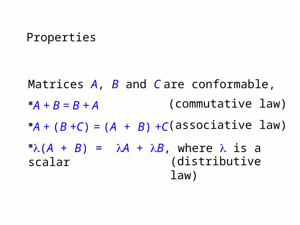
Properties

Matrices A, B and C are conformable,

A + B = B + A

A + (B +C) = (A + B) +C

(A + B) = A + B, where is a scalar

(commutative law)

(associative law)

(distributive law)

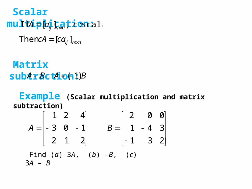
Example (Scalar multiplication and matrix subtraction)

212

103

421

A

231

341

002

B

Find (a) 3A, (b) –B, (c) 3A – B

Scalar multiplication:scalar : ,][ If caA nmij

nmijcacA ][Then

Matrix subtraction:BABA )1(

(a)

212

103

421

33A

(b)

231

341

002

1B

(c)

231

341

002

636

309

1263

3 BA

Sol:

636

309

1263

231323

130333

432313

231

341

002

407

6410

1261

Matrix Multiplication

The above inhomogeneous equations can be written similarly

We now write linear equations in terms of matrices because their coefficients represent an array of numbers that we just defined as a matrix,

1 2 3

1 2 3

1 2 3

3 2 11

2 3 13

4 12

x x x

x x x

x x x

3 2

1 3

4 2

5 0

A

2 2

3 2

4 1B

Example : (Multiplication of Matrices)

Sol:

)1)(0()2)(5()4)(0()3)(5(

)1)(2()2)(4()4)(2()3)(4(

)1)(3()2)(1()4)(3()3)(1(

AB

1015

64

19

1 2 3

0 1 4A

1 2

2 3

5 0

B

11

12

21

22

1 ( 1) 2 2 3 5 181 2

1 2 2 3 3 0 81 2 32 3

0 ( 1) 1 2 4 5 220 1 45 0

0 2 1 3 4 0 3

c

c

c

c

1 21 2 3 18 8

2 30 1 4 22 3

5 0

C AB

Properties

Matrices A, B and C are conformable,

A(B + C) = AB + AC

(A + B)C = AC + BC

A(BC) = (AB) C

AB BA in general

AB = 0 NOT necessarily imply A = 0 or B = 0

AB = AC NOT necessarily imply B = C How

ever

Transpose of a matrix:

nm

mnmm

n

n

M

aaa

aaa

aaa

A

If

21

22221

11211

mn

mnnn

m

m

T M

aaa

aaa

aaa

A

Then

21

22212

12111

AA TT )( )1(

TTT BABA )( )2(

)()( )3( TT AccA

)( )4( TTT ABAB

Properties of transposes:

Matrix Inversion

We cannot define division of matrices, but for a square matrix A with nonzero determinant we can find a matrix A−1, called the inverse of A, so that

A−1A = AA−1 = I.

If B and C are both inverses of the matrix A, then B = C.

Proof:

CB

CIB

CBCA

CIABC

IAB

)(

)(

Consequently, the inverse of a matrix is unique.

Notes:(1) The inverse of A is denoted by 1A

IAAAA 11 )2(

Theorem : (The inverse of a matrix is unique)

6 2 3

1 1 0

1 0 1

B

Show B is the the inverse of matrix A.

1 2 3

1 3 3

1 2 4

A

Example:

1 0 0

0 1 0

0 0 1

AB BA

Ans: Note that

33

Inverse of a 33 matrix

Cofactor matrix of A

1 2 3

0 4 5

1 0 6

A

The cofactor for each element of matrix A:

11

4 524

0 6A 12

0 55

1 6A 13

0 44

1 0A

21

2 312

0 6A 22

1 33

1 6A 23

1 22

1 0A

31

2 32

4 5A 32

1 35

0 5A 33

1 24

0 4A

11 12 13

21 22 23

31 32 33

A A A

CFM of A A A A

A A A

34

Cofactor matrix of is then given by:1 2 3

0 4 5

1 0 6

A

24 5 4

12 3 2

2 5 4

1 2 34 5 0 5 0 4

det 0 4 5 1 2 30 6 1 6 1 0

1 0 6

det 1(24 0) 2(0 5) 3(0 4) 24 10 12 22

35

Inverse matrix of is given by:1 2 3

0 4 5

1 0 6

A

1

24 5 4 24 12 21 1

12 3 2 5 3 522

2 5 4 4 2 4

T

AA

12 11 6 11 1 11

5 22 3 22 5 22

2 11 1 11 2 11

Simple C Program

/* A first C Program*/

#include <stdio.h>

void main()

{ printf("Happy New Year 2014 \n");

}

Matrix multiplication in c language

1 Requirements

Design, develop and execute a program in C to read two matrices A (m x n) and

B (p x q) and compute the product of A and B if the matrices are compatible for

multiplication. The program must print the input matrices and the resultant matrix

with suitable headings and format if the matrices are compatible for multiplication,

otherwise the program must print a suitable message. (For the purpose of

demonstration, the array sizes m, n, p, and q can all be less than or equal to 3)

2 Analysis

c[i, j] = a[i,k] b[k,j]

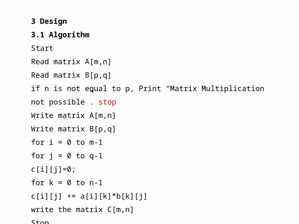
3 Design

3.1 Algorithm

Start

Read matrix A[m,n]

Read matrix B[p,q]

if n is not equal to p, Print “Matrix Multiplication not possible”. stop

Write matrix A[m,n]

Write matrix B[p,q]

for i = 0 to m-1

for j = 0 to q-1

c[i][j]=0;

for k = 0 to n-1

c[i][j] += a[i][k]*b[k][j]

write the matrix C[m,n]

Stop

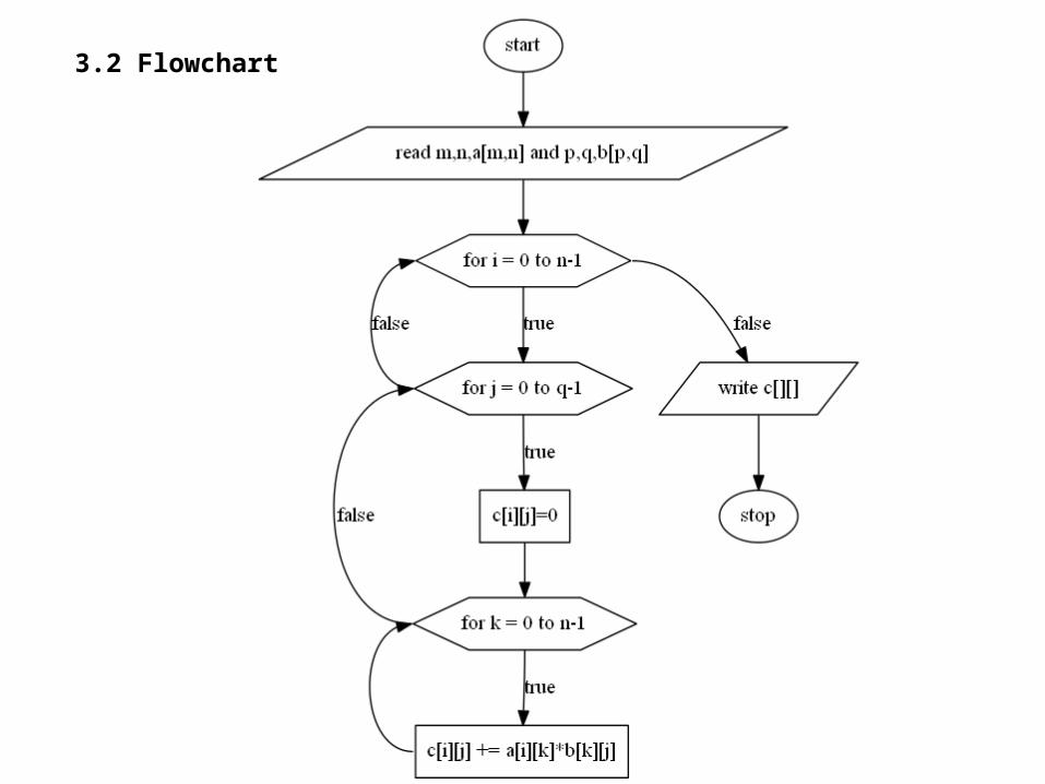
3.2 Flowchart

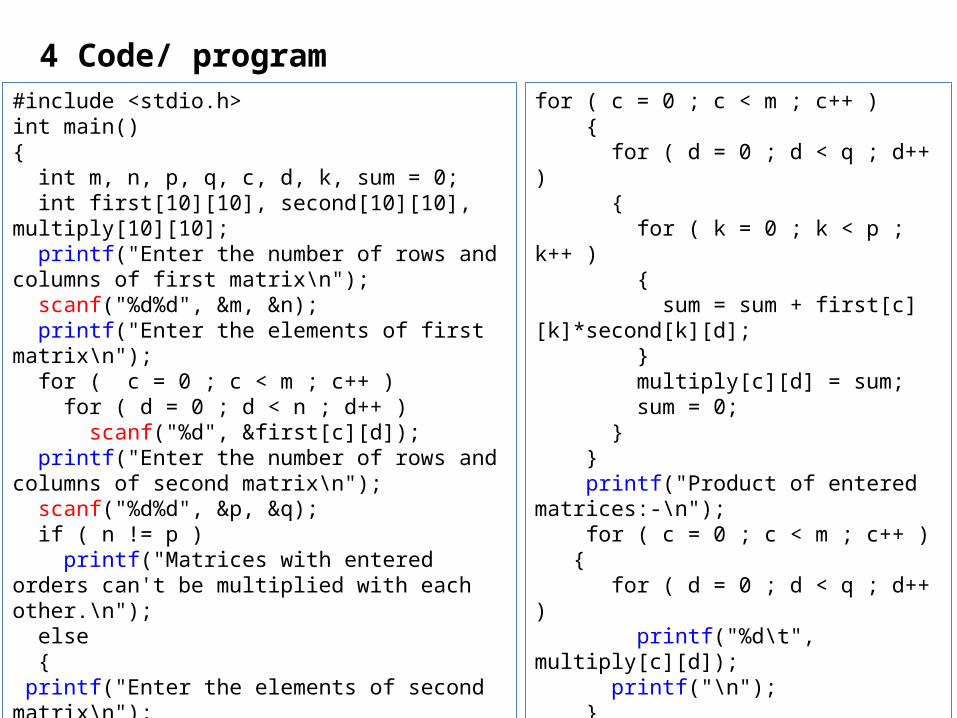
4 Code/ program#include <stdio.h>int main(){ int m, n, p, q, c, d, k, sum = 0; int first[10][10], second[10][10], multiply[10][10]; printf("Enter the number of rows and columns of first matrix\n"); scanf("%d%d", &m, &n); printf("Enter the elements of first matrix\n"); for ( c = 0 ; c < m ; c++ ) for ( d = 0 ; d < n ; d++ ) scanf("%d", &first[c][d]); printf("Enter the number of rows and columns of second matrix\n"); scanf("%d%d", &p, &q); if ( n != p ) printf("Matrices with entered orders can't be multiplied with each other.\n"); else { printf("Enter the elements of second matrix\n"); for ( c = 0 ; c < p ; c++ ) for ( d = 0 ; d < q ; d++ ) scanf("%d", &second[c][d]);

for ( c = 0 ; c < m ; c++ ) { for ( d = 0 ; d < q ; d++ ) { for ( k = 0 ; k < p ; k++ ) { sum = sum + first[c][k]*second[k][d]; } multiply[c][d] = sum; sum = 0; } } printf("Product of entered matrices:-\n"); for ( c = 0 ; c < m ; c++ ) { for ( d = 0 ; d < q ; d++ ) printf("%d\t", multiply[c][d]); printf("\n"); } } return 0;}

=MINVERSE(A2:C4)

=MMULT(array1,array2)

=MDETERM(array)

=TRANSPOSE(A2:C2)

12 11 6 11 1 11

5 22 3 22 5 22

2 11 1 11 2 11

C code to find inverse of a matrix

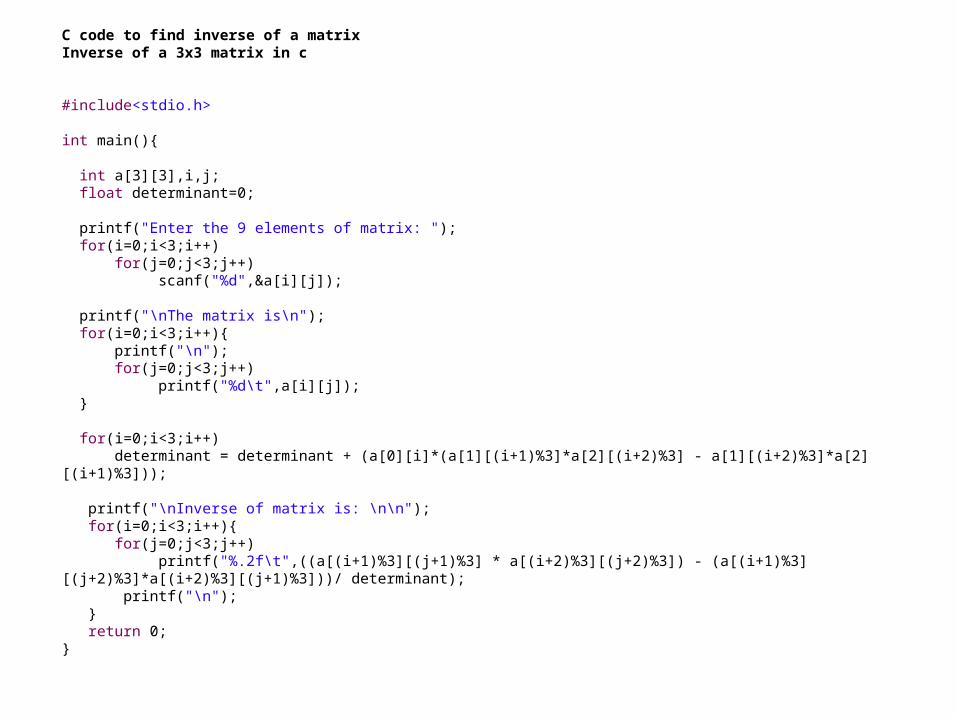
C code to find inverse of a matrixInverse of a 3x3 matrix in c

#include<stdio.h>

int main(){

  int a[3][3],i,j;  float determinant=0;

  printf("Enter the 9 elements of matrix: ");  for(i=0;i<3;i++)      for(j=0;j<3;j++)           scanf("%d",&a[i][j]);

  printf("\nThe matrix is\n");  for(i=0;i<3;i++){      printf("\n");      for(j=0;j<3;j++)           printf("%d\t",a[i][j]);  }

  for(i=0;i<3;i++)      determinant = determinant + (a[0][i]*(a[1][(i+1)%3]*a[2][(i+2)%3] - a[1][(i+2)%3]*a[2][(i+1)%3]));

   printf("\nInverse of matrix is: \n\n");   for(i=0;i<3;i++){      for(j=0;j<3;j++)           printf("%.2f\t",((a[(i+1)%3][(j+1)%3] * a[(i+2)%3][(j+2)%3]) - (a[(i+1)%3][(j+2)%3]*a[(i+2)%3][(j+1)%3]))/ determinant);       printf("\n");   }   return 0;}

Example

Find (a) the eigenvalues and (b) the eigenvectors of the matrix

21

45

Solution: (a) The eigenvalues: The characteristic equation is

0)1)(6(

067

042510

04)2)(5(

021

45)det(

2

2

IA

1 and 6 21 which has two roots

(b) The eigenvectors: For = 1 = 6 the system for eigen vectors assumes the form: (A I) X = 0 i.e. (A 6I) X = 0

0)(

0 )(

0 )(

2211

2222121

1212111

nnnnn

nn

nn

xaxaxa

xaxaxa

xaxaxa

0)62(

04)65(

21

21

xx

xx04

04

21

21

xx

xx

Thus x1 = 4x2, and

1

41X

For = 2 = 1 the system for eigen vectors assumes the form

0)12(

04)15(

21

21

xx

xx0

044

21

21

xx

xx

Thus x1 = x2, and

1

12X

11

14S

41

11CfS514det S

41

11TCfS

41

11511S

1 1 1 5 4 4 1 6 01 5

1 4 1 2 1 1 0 1S AS

21

45A

ExampleFind a matrix S that diagonalizes

500

032

023

A

Solution: We have first to find the eigenvalues and the corresponding eigen-vectors of matrix A. The characteristic equation of A is

3 2 0

2 3 0 0

0 0 5

0)5)(1( 2

so that the eigenvalues of A are = 1 and = 5.

If = 5 the equation (I A) X = 0 becomes

0

0

0

5500

0352

0235

3

2

1

x

x

x

0

0

0

000

022

022

3

2

1

x

x

x

0

0

0

000

022

022

321

321

321

xxx

xxx

xxx Solving this system yieldsx1 = s; x2 = s; x3 = t;where s and t are arbitrary values.

Thus the eigenvectors of A corresponding to = 5 are the non-zero vectors of the form

1

0

0

0

1

1

0

0

0

ts

t

s

s

t

s

s

X

since

are linearly independent, they are eigenvectors corresponding to = 5

1

0

0

and

0

1

1

for = 1 we have

0

0

0

5100

0312

0231

3

2

1

x

x

x

0

0

0

400

022

022

3

2

1

x

x

x

0

0

0

400

022

022

321

321

321

xxx

xxx

xxx Solving this system yieldsx1 = t; x2 = t; x3 = 0;where t is arbitrary.

Thus the eigenvectors of A corresponding to = 1 are the non-zero vectors of the form

0

1

1

0

tt

t

X

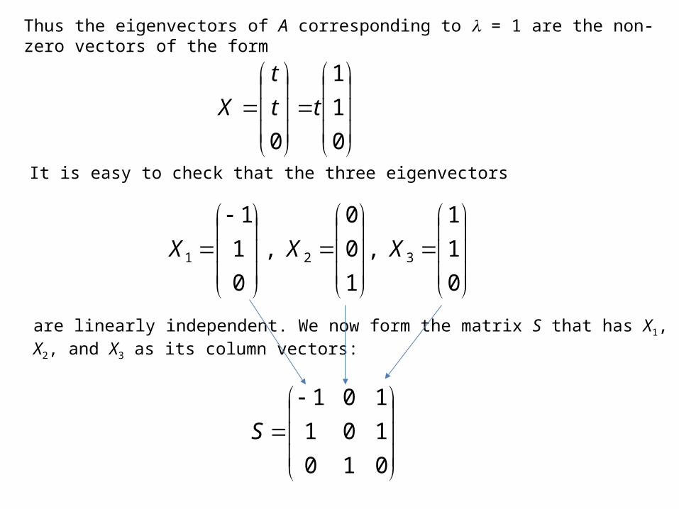
It is easy to check that the three eigenvectors

are linearly independent. We now form the matrix S that has X1, X2, and X3 as its column vectors:

0

1

1

,

1

0

0

,

0

1

1

321 XXX

010

101

101

S

The matrix S1AS is diagonal:

100

050

005

010

101

101

500

032

023

02/12/1

100

02/12/11ASS

There is no preferred order for the columns of S. If had we written

100

011

011

S

then we would have obtained (verify)

100

050

0051ASS

ExampleFind eigenvalues and eigenvectors of the following matrix and diagonalize it:

cossin

sincosT

ii ee 21 ,

i

Xi

X1

2/1~

1

2/1~

21

2/2/1

2/2/1

2/2/

2/12/1 †

i

iU

iiU

i

i

e

eTUU

0

0†

Chapter 3

Matrix Algebra

3.1 Introduction3.2 Types of Matrices3.3 Simple Matrix Problems

3.3.1 Addition and Subtraction3.3.2 Multiplication of Matrices

3.4 Elliptic Equations —Poisson’s Equation3.4.1 One Dimension3.4.2 2 or more Dimensions

3.5 Systems of Equations and Matrix Inversion3.5.1 Exact Methods3.5.2 Iterative Methods

The Jacobi MethodThe Gauss–Seidel Method

3.6 Matrix Eigenvalue Problems3.6.1 Schrodinger’s equation3.6.2 General Principles3.6.3 Full Diagonalisation3.6.4 The Generalised Eigenvalue Problem3.6.5 Partial Diagonalisation3.6.6 Sparse Matrices and the Lanczos Algorithm

Types of Matrices

Hermitian Matrices

Real Symmetric Matrices

Positive Definite Matrices

Unitary Matrices

Diagonal Matrices

Tridiagonal Matrices

Upper and Lower Triangular Matrices

Sparse Matrices

General Matrices

Complex Symmetric Matrices

Symplectic Matrices

There are several ways of classifying matrices depending on symmetry, sparsity etc.

Here we provide a list of types of matrices and the situation in which they may arise in physics.

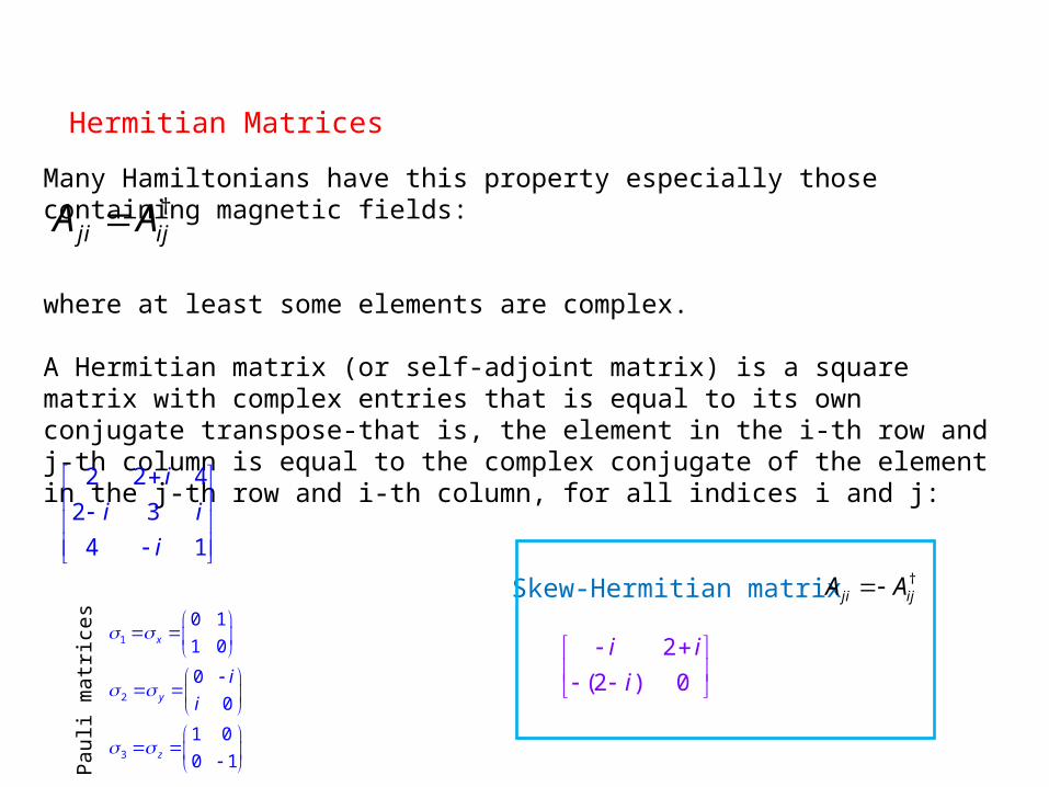
Hermitian Matrices

Many Hamiltonians have this property especially those containing magnetic fields:

where at least some elements are complex.

A Hermitian matrix (or self-adjoint matrix) is a square matrix with complex entries that is equal to its own conjugate transpose-that is, the element in the i-th row and j-th column is equal to the complex conjugate of the element in the j-th row and i-th column, for all indices i and j:

†ji ijA A

Skew-Hermitian matrix †ji ijA A

2 2 4

2 3

4 1

i

i i

i

Pau

li m

atric

es 1

2

3

0 1

1 0

0

0

1 0

0 1

x

y

z

i

i

2

(2 ) 0

i i

i

Real Symmetric Matrices

These are the commonest matrices in physics as most Hamiltonians can be represented this way: And all Aij are real. This is a special case of Hermitian

matrices.

a symmetric matrix is a square matrix that is equal to its transpose. Formally, matrix A is symmetric if A = AT.

ji ijA A

1 7 3

7 4 5

3 5 6

Positive Definite Matrices

A special sort of Hermitian matrix in which all the eigenvalues are positive. The overlap matrices used in tight–binding electronic structure calculations are like this.Sometimes matrices are non–negative definite and zero eigenvalues are also allowed. An example is the dynamical matrix describing vibrations of the atoms of a molecule or crystal, where 2 0.

2 1 0

1 2 1

0 1 2

M

Unitary Matrices

A complex square matrix U is unitary ifU* U = U U* = I ,where I is the identity matrix and U* is the conjugate transpose of U. The real analogue of a unitary matrix is an orthonormal matrix.

1 11

1 12

i iA

i i

2

1 1 1 1 4 0 1 01 1 1*

1 1 1 1 0 4 0 12 2 4

i i i iAA I

i i i i

Show that the following matrix is unitary.

We conclude that A* = A– 1 . Therefore, A is a unitary matrix.

A−1A = AA−1 = I

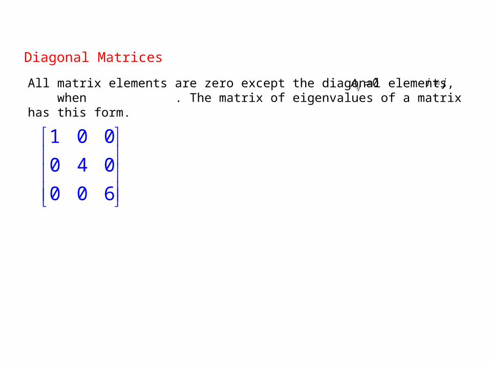
Diagonal Matrices

All matrix elements are zero except the diagonal elements, when . The matrix of eigenvalues of a matrix has this form.

0ijA i j

1 0 0

0 4 0

0 0 6

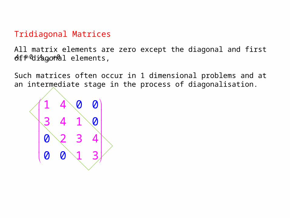
Tridiagonal Matrices

All matrix elements are zero except the diagonal and first off diagonal elements,

Such matrices often occur in 1 dimensional problems and at an intermediate stage in the process of diagonalisation.

, , 10 0i i i iA A

1 4

3 4 1

2 3 4

1

0 0

0

0

0 0 3

Upper and Lower Triangular Matrices

In Upper Triangular Matrices all the matrix elements below the diagonal are zero, . A Lower Triangular Matrix is the other way round,

These occur at an intermediate stage in solving systems of equations and inverting matrices.

0 ijA i j 0 ijA i j

1 4 2

30 4

0 0 1

1

2 8

0 0

0

4 9 7

Sparse Matrices

Matrices in which most of the elements are zero according to some pattern. In general sparsity is only useful if the number of non–zero matrix elements of an N x N matrix is proportional to N rather than N2. In this case it may be possible to write a function which will multiply a given vector x by the matrix A to give Ax without ever having to store all the elements of A. Such matrices commonly occur as a result of simple discretisation of partial differential equations, and in simple models to describe many physical phenomena.

              0     0   6     0    9   0   0              2     0   0     7    8   0   4              10   0   0     0    0   0   0              0     0   12   0    0   0   0              0     0   0     0    0   0   0              0     0   0     3    0   0   5

General Matrices

Any matrix which doesn’t fit into any of the above categories, especially non–square matrices.

Complex Symmetric Matrices

Not generally a useful symmetry. There are however two related situations in which these occur in theoretical physics: Green’s functions and scattering (S) matrices.In both these cases the real and imaginary parts commute with each other, but this is not true for a general complex symmetric matrix.

There are a few extra types which arise less often:

2 1

1 0

iA

5 1

2

1 3

i

T i i

i

Symplectic Matrices

a symplectic matrix is a 2n×2n matrix M with real entries that satisfies the conditionMT M = .where MT denotes the transpose of M and is a fixed 2n×2n nonsingular, skew-symmetric matrix. This definition can be extended to 2n×2n matrices with entries in other fields, e.g. the complex numbers.Typically Ω is chosen to be the block matrix.

A second-order partial differential equation,

is called elliptic if the matrix is positive definite.

The basic example of an elliptic partial differential equation is Laplace's equation in  n-dimensional Euclidean space, where the Laplacian is defined by

Other examples of elliptic equations include the nonhomogeneous Poisson's equation and the non-linear minimal surface equation.

2 0xx xy yy x yAu Bu Cu Du Eu F A B

ZB C

2 0u

22

21

n

i ix

2 ( )u f x

2 2 2

2 20

u u u u uA B C D E F

x x y y x y

Elliptic equations-Poisson’s equation

2 2 2

2 2 2( )

d V d V d Vf x

dx dy dz

One Dimension

We start by considering the one dimensional Poisson's equation

The 2nd derivative may be discretised in the usual way to give

where we define

The boundary conditions are usually of the form although sometimes the condition is on the first derivative. Since Vo and VN+1 are both known the n = 1 and n = N above equations may be written as

2

2( )

d Vf x

dx

21 12n n n nV V V x f

( )n nf f x x n x

1 1( ) at and ( ) at . o o N NV x V x x V x V x x

2 4

21 2 1

21 2 3 2

22 3 4 3

21 1

2

2

2

2

o

N N N N

V V x f V

V V V x f

V V V x f

V V x f V

21 12n n n nV V V x f

1

2

3

n

n

n

n N

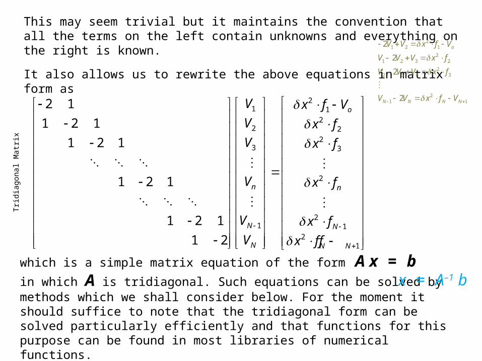
It also allows us to rewrite the above equations in matrix form as

21 1

22 2

23 3

2

21 1

21

2 1

1 2 1

1 2 1

1 2 1

1 2 1

1 2

o

n n

N N

N N N

V x f V

V x f

V x f

V x f

V x f

V x f f

which is a simple matrix equation of the form A x = bin which A is tridiagonal. Such equations can be solved by methods which we shall consider below. For the moment it should suffice to note that the tridiagonal form can be solved particularly efficiently and that functions for this purpose can be found in most libraries of numerical functions.

x = A–1 b

21 2 1

21 2 3 2

22 3 4 3

21 1

2

2

2

2

o

N N N N

V V x f V

V V V x f

V V V x f

V V x f V

This may seem trivial but it maintains the convention that all the terms on the left contain unknowns and everything on the right is known.

Trid

iago

nal M

atrix

We could only write the equation in this matrix form because the boundary conditions allowed us to eliminate a term from the 1st and last lines.

Periodic boundary conditions, such as V (x + L) = V (x) can be implemented, but they have the effect of adding a non-zero element to the top right and bottom left of the matrix, A1N and AN1, so that the tridiagonal form is lost.

It is sometimes more efficient to solve Poisson's or Laplace's equation using Fast Fourier Transformation (FFT). Again there are efficient library routines available (Numerical Algorithms Group, n.d.). This is especially true in machines with vector processors.

2 or more Dimensions

Poisson's and Laplace's equations can be solved in 2 or more dimensions by simple generalisations of the schemes discussed for 1D. However the resulting matrix will not in general be tridiagonal. The discretised form of the equation takes the form

The 2 dimensional index pairs {m, n} may be mapped on to one dimension for the purpose of setting up the matrix. A common choice is so-called dictionary order,

Alternatively Fourier transformation can be used either for all dimensions or to reduce the problem to tridiagonal form.

2, 1 , 1 1, 1, , ,4m n m n m n m n m n m nV V V V V x f

21 12n n n nV V V x f

(1,1), (1, 2),......(1, ), (2,1), (2, 2),....(2, ),...( ,1), ( , 2),...( , )N N N N N N

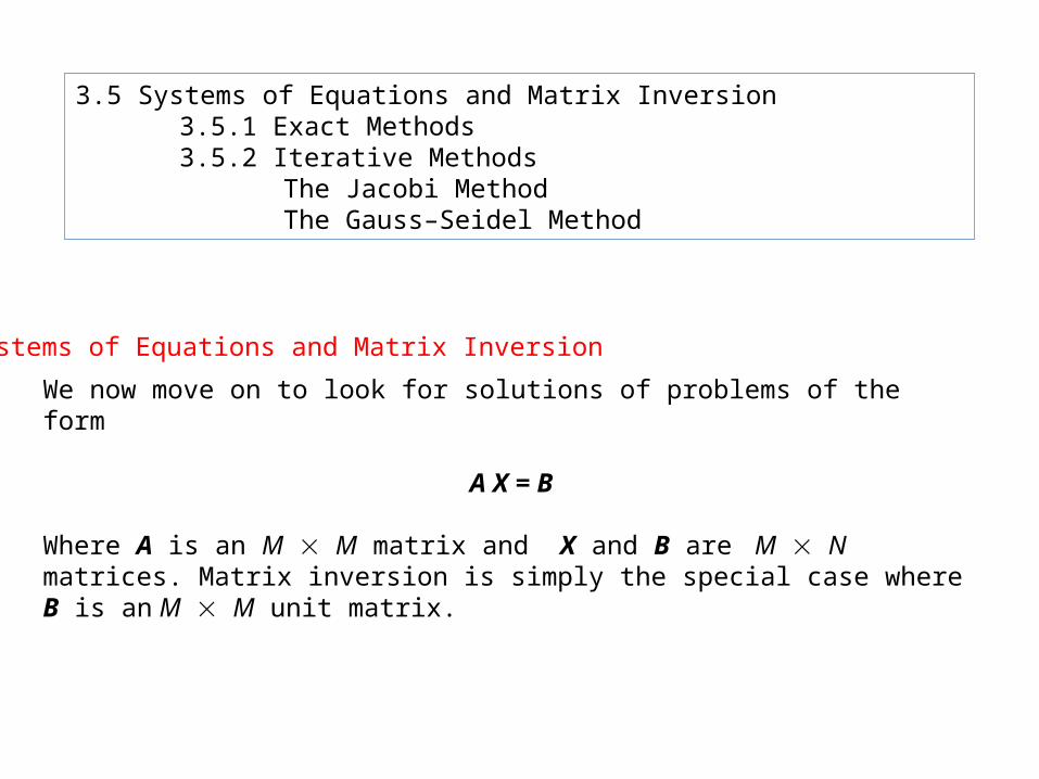
Systems of Equations and Matrix Inversion

We now move on to look for solutions of problems of the form 

A X = B

Where A is an M M matrix and  X and B are  M N matrices. Matrix inversion is simply the special case where B is an M M unit matrix.

3.5 Systems of Equations and Matrix Inversion3.5.1 Exact Methods3.5.2 Iterative Methods

The Jacobi MethodThe Gauss–Seidel Method

Direct (exact) methods:

Examples: Gaussian elimination,LU factorizations, matrix inversion, etc.

Always give an answer. Deterministic.

Robust. No convergence analysis.

Great for multiple right hand sides.

Have often been considered too slow for high performance computing.

(Directly access elements or blocks of A.)

(Exact except for rounding errors.)

Iterative methods:

Examples: GMRES, conjugate gradients, Gauss-Seidel, etc.

Construct a sequence of vectorsu1, u2, u3, . . . that (hopefully!) converge to the exact solution.

Many iterative methods access A only via its action on vectors.

Often require problem specific pre-conditioners.

High performance when they work well.O(N) solvers.

"direct" versus "Iterative" solvers

Two classes of methods for solving an N × N linear algebraic system

A X = B

Most library routines, for example those in the NAG (Numerical Algorithms Group, n.d.) or LaPack (Lapack Numerical Library, n.d.) libraries are based on some variation of Gaussian elimination. The standard procedure is to call a first function which performs an LU decomposition of the matrix A , 

A = LU

where L and U are lower and upper triangular matrices respectively, followed by a function which performs the operations 

Y = L–1 BX = U–1 Y

on each column of B.

The procedure is sometimes described as Gaussian Elimination. A common variation on this procedure is partial pivoting. This is a trick to avoid numerical instability in the Gaussian Elimination (or LU decomposition) by sorting the rows of A to avoid dividing by small numbers.

Exact Methods

There are several aspects of this procedure which should be noted:

The  LU  decomposition is usually done in place, so that the matrix  A  is overwritten by the matrices  L  and  U .The matrix  B is often overwritten by the solution  X .A well written  LU decomposition routine should be able to spot when  A is singular and return a flag to tell you so.Often the  LU decomposition routine will also return the determinant of  A .Conventionally the lower triangular matrix  L is defined such that all its diagonal elements are unity. This is what makes it possible to replace  A  with both  L  and  U .Some libraries provide separate routines for the Gaussian Elimination and the Back-Substitution steps. Often the Back-Substitution must be run separately for each column of  B .Routines are provided for a wide range of different types of matrices. The symmetry of the matrix is not often used however.

The time taken to solve  N  equations in N  unknowns is generally proportional to  N3  for the Gaussian-Elimination (  LU -decomposition) step. The Back-Substitution step goes as  N2 for each column of  B . As before this may be modified by parallelism.

Sets of Linear EquationsGaussian Elimination: Successive Elimination of Variables

Our problem is to solve a set of linear algebraic equations. For the time being wewill assume that a unique solution exists and that the number of equations equalsthe number of variables.Consider a set of three equations:

The basic idea of the Gaussian elimination method is the transformation of this setof equations into a staggered set:

Klaus Weltner · Wolfgang J. Weber · Jean Grosjean Peter SchusterMathematics for Physicists and Engineers pp441

11 1 12 2 13 3 1

21 1 22 2 23 3 2

31 1 32 2 33 3 3

a x a x a x b

a x a x a x b

a x a x a x b

11 1 12 2 13 3 1

22 2 23 3 2

33 3 3

a x a x a x b

a x a x b

a x b

All coefficients a’ij below the diagonal are zero. The solution in this case is straightforward.The last equation is solved for x3. Now, the second can be solved by insertingthe value of x3. This procedure can be repeated for the uppermost equation.

The question is how to transform the given set of equations into a staggered set.This can be achieved by the method of successive elimination of variables. Thefollowing steps are necessary:

1. We have to eliminate x1 in all but the first equation. This can be done by subtractinga21/a11 times the first equation from the second equation and a31/a11

times the first equation from the third equation.

2. We have to eliminate x2 in all but the second equation. This can be done bysubtracting a32/a22 times the second equation from the third equation.

3. Determination of the variables. Starting with the last equation in the set andproceeding upwards, we obtain first x3, then x2, and finally x1.

This procedure is called the Gaussian method of elimination. It can be extended tosets of any number of linear equations.

Example We can solve the following set of equations according to the proceduregiven:

1. Elimination of x1. We multiply Eq. [1] by 3/6 and subtract it from Eq. [2]. Thenwe multiply Eq. [1] by 2/6 and subtract it from Eq. [3]. The result is

2. Elimination of x2. We multiply Eq. [2’] by 2 and add it to Eq. [3’]. The result is

1 2 3

1 2 3

1 2

6 12 6 6

3 5 5 13

2 6 0 10

x x x

x x x

x x

[1]

[2]

[3]

[1]

[2 ]

[3 ]

1 2 3

2 3

2 3

6 12 6 6

2 10

2 2 12

x x x

x x

x x

[1 ]

[2 ]

[3 ]

1 2 3

2 3

3

6 12 6 6

2 10

2 8

x x x

x x

x

3. Determination of the variables x1, x2, x3. Starting with the last equation in the set, we obtain

Now Eq. [2] can be solved for x2 by inserting the value of x3. Thus

This procedure is repeated for Eq. [1] giving

3

84

2x

2 2x

1 1x

Flow chart & C program of Gauss Elimination Method

/* Gauss elimination method */ # include <studio.h)# define N 4 main ( ) { float a[N] [N+1] ,x[N] , t, s; int i, j, k ; print f (“enter the elements of the augmented matrix row wise \n”) ; for( i=0 ; i<N; i++ ) for (j=0; j<N+1 ; j++) Scan f (“% f” ,& a [i] , [j] ); for (j=0; j<N-1; j++) for (i= j+1; i<N ; i++){ t= a[i] [j] /a[j] [j];for (k=0; k<N+1; k++) a [i] [k] =a [j] [k] *t;}/* now printing the upper triangular matrix */ print f(“The upper triangular matrix is :- /n”) for ( i=0 ; i<N ;i++){for (j=0; j<N+1 ; j++) print f (“%8 . 4f “ , a [i] [j] ) :print f (“\n”);}/* now performing back substitution */ for (i=N-1 ; i>=0 ; i- -) {s= 0 ; for (j=i+1 ; j<N; j++ ) s + = a[i] [j] *x[j] ; x[i] = (a[i] [N –s )/a [i] [i] ; } /* now printing the results */print f (“ The solution is :- /n”) ; for (i=0 ; i<N; i++) print f (“x[%3d] = %7 . 4f \n “ , i+1, x[i]) ;}

Gauss–Jordan Elimination

Let us consider whether a set of n linear equations with n variables can be transformedby successive elimination of the variables into the form

The transformed set of equations gives the solution for all variables directly. Thetransformation is achieved by the following method, which is basically an extensionof the Gaussian elimination method.

At each step, the elimination of xj has to be carried out not only for the coefficientsbelow the diagonal, but also for the coefficients above the diagonal. In addition, the equation is divided by the coefficient ajj .

This method is called Gauss–Jordan elimination.

1 1

2 2

3 3

0 0 0

0 0 0

0 0 0

0 0 0 n n

x C

x C

x C

x C

We show the procedure by using the previous example.This is the set

To facilitate the numerical calculation, we will begin each step by dividing the respectiveequation by ajj .

1. We divide the first equation by a11 = 6 and eliminate x1 in the other two equations.

Second equation: we subtract 3× first equationThird equation: we subtract 2× first equation

This gives

1 2 3

1 2 3

1 2

6 12 6 6

3 5 5 13

2 6 0 10

x x x

x x x

x x

[1]

[2]

[3]

1 2 3

2 3

2 3

2 1

0 2 10

0 2 2 12

x x x

x x

x x

2. We eliminate x2 above and below the diagonal.

Third equation: we add 2× second equationFirst equation: we add 2× second equation

This gives

3. We divide the third equation by a33 and eliminate x3 in the two equations above it.

Second equation: we subtract 2× third equationFirst equation: we subtract 5× third equation

This gives

This results in the final form which shows the solution.

[1 ]

[2 ]

[3 ]

1 3

2 3

3

0 5 21

0 2 10

0 0 2 8

x x

x x

x

[1 ]

[2 ]

[3 ]

1

2

3

0 0 1

0 0 2

0 0 4

x

x

x

4 3 13

2 3

7 3 0

x y z

x y z

x y z

4 3 1 13

2 1 1 3

7 1 3 0

1 3 / 4 1/ 4 13 / 4

2 1 1 3

7 1 3 0

1 3 / 4 1/ 4 13 / 4

0 5 / 2 3 / 2 19 / 2

0 17 / 4 19 / 4 91/ 4

1 3 / 4 1/ 4 13 / 4

0 1 3 / 5 19 / 5

0 17 / 4 19 / 4 91/ 4

Do by another example

Form augmented coefficient matrix

Multiply ¼ to make upper left corner (a11) = 1 (First Equation)

Multiply first row by 2 and subtract from 2nd rowMultiply first row by 7 and subtract from 3rd row

Multiply 2nd row by (-2/5)

1 0 1/ 5 2 / 5

0 1 3 / 5 19 / 5

0 0 11/ 5 33 / 5

1 0 1/ 5 2 / 5

0 1 3 / 5 19 / 5

0 0 1 3

1 0 0 1

0 1 0 2

0 0 1 3

1 0 0 1

0 1 0 2

0 0 1 3

x y z

x y z

x y z

Multiply 2nd row by ¾ and subtract from 1st rowMultiply 2nd row by 17/4 and add to 3rd row

Multiply 3rd row by -5/11 to make a33 = 1

Multiply 3rd row by 3/5 and subtract from 2nd rowMultiply 3rd row by 1/5 and add to 1st row

Now rewrite equations as

/* Gauss Jordan method */

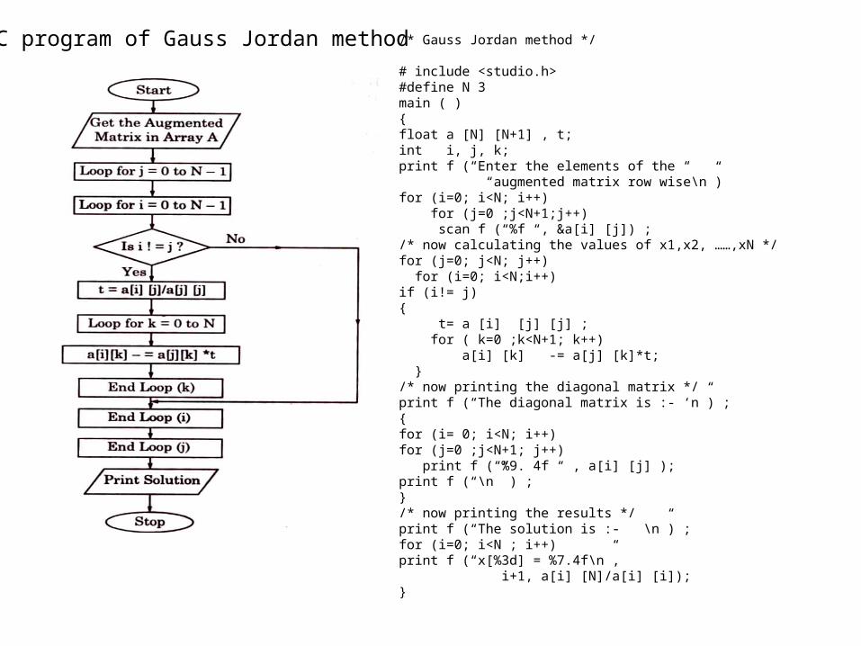
# include <studio.h>#define N 3main ( ) {float a [N] [N+1] , t; int i, j, k; print f (“Enter the elements of the “ “augmented matrix row wise\n”)for (i=0; i<N; i++) for (j=0 ;j<N+1;j++) scan f (“%f “, &a[i] [j]) ;/* now calculating the values of x1,x2, ……,xN */for (j=0; j<N; j++) for (i=0; i<N;i++)if (i!= j) { t= a [i] [j] [j] ; for ( k=0 ;k<N+1; k++) a[i] [k] -= a[j] [k]*t; }/* now printing the diagonal matrix */ print f (“The diagonal matrix is :- ‘n”) ;{for (i= 0; i<N; i++) for (j=0 ;j<N+1; j++) print f (“%9. 4f “ , a[i] [j] ); print f (“\n” ) ;}/* now printing the results */ print f (“The solution is :- \n”) ; for (i=0; i<N ; i++)print f (“x[%3d] = %7.4f\n”, i+1, a[i] [N]/a[i] [i]); }

C program of Gauss Jordan method

Iterative MethodsAs an alternative to the above library routines, especially when large sparse matrices are involved, it is possible to solve the equations iteratively.

The Jacobi Method

It is an algorithm for determining the solutions of a system of linear equations with largest absolute values in each row and column dominated by the diagonal element. Each diagonal element is solved for, and an approximate value plugged in. The process is then iterated until it converges.

A X = BX = A–1B

We first divide the matrix A into 3 parts A = D + L + U

Where D is a diagonal matrix (i.e. ) and L and U are strict lower and upper triangular matrices respectively (i.e. ). We now write the Jacobi or Gauss-Jacobi iterative procedure to solve our system of equations as

Xn+1 = D 1 [B (L + U) Xn]where the superscripts n refer to the iteration number. Note that in practice this procedure requires the storage of the diagonal matrix, D, and a function to multiply the vector, Xn by L + U .

0 for ijD i j

0 for all ii iiL U i

1 4 5 3 0 0 0 0 0 0 0 0

3 4 1 6 0 0 0 0 0 0 0 0

4 2 3 4 0 0 0 0 0 0 0 0

7 3 1 3 0 0 0 0 0 0 0

1

4

3

3

4 2

7

4 5 3

1 6

3 3 0

4

1

(D + L + U) X = BD X + (L +U)X = BD X = B – (L +U) X

X = D –1 [ B – (L +U) X ]

int i;const int N = ??; // incomplete codedouble xa[N], xb[N], b[N];while ( ... ) // incomplete code{for ( i = 0; i < N; i++ )xa[i] = (b[i] - xb[i-1] - xb[i+1]) * 0.5;for ( i = 0; i < N; i++ )xb[i] = xa[i];}

Simple C code to implement this for a 1D Poisson’s equation is given below.

Any implementation of the Jacobi Method above will involve a loop over the matrix elements in each column of Xn+1. Instead of calculating a completely new matrix Xn+1 at each iteration and then replacing Xn with it before the next iteration, as in the above code, it might seem sensible to replace the elements of Xn with those of Xn+1 as soon as they have been calculated. Naïvely we would expect faster convergence. This is equivalent to rewriting the Jacobi equation as

Xn+1 = (D + L)1 [B U Xn]

This Gauss-Seidel method has better convergence than the Jacobi method, but only marginally so.

Gauss-Seidel Method

A X = BX = A–1B

(D + L + U) X = B(D + L) X + U X = B(D + L) X = B – U X

X = (D + L) –1 [ B – U X ]

11 1 12 2 13 3 1 1

21 1 22 2 23 3 2 2

31 1 32 2 33 3 3 3

1 1 2 2 3 3

n n

n n

n n

n n n nn n n

a x a x a x a x C

a x a x a x a x C

a x a x a x a x C

a x a x a x a x C

1 12 2 13 3 11

11

2 21 1 23 3 22

22

3 31 1 32 2 33

33

1 1 2 2 3 3 , 1 1

n n

n n

n n

n n n n n n nn

nn

C a x a x a xx

a

C a x a x a xx

a

C a x a x a xx

a

C a x a x a x a xx

a

Elimination methods can be used for m = 25 - 50. Beyond this, round off errors, computing time etc. kill you.

Instead we use Gauss-Seidel Method for larger m.

Guess a root=> iteration=> improve root.

Assume we have a set of equations

[A] [X] = [C]

Gauss-Seidel Method

Guess x2, x3, ....... xn = 0

Calculate x1

Substitute x1 into x2 equation, calculate x2

...

...

...

Calculate xm

Use calculated values to cycle again until process converges.

1 2 3

1 2 3

1 2 3

3 0.1 0.2 7.85

0.1 7 0.3 19.3

0.3 0.2 10 71.4

x x x

x x x

x x x

2 31

1 32

1 23

7.85 0.1 0.2

319.3 0.1 0.3

771.4 0.3 0.2

10

x xx

x xx

x xx

1

7.852.62

3x

2

19.3 0.1 2.62 02.79

7x

3

71.4 0.3 2.62 0.2 2.797.005

10x

Example

Rewriting equations

Answer: Put x2 = x3 = 0

Substitute in x2

Put into x3 equation

Cycle over

1

7.85 0.1 2.79 0.2 7.005

32.99x

1

2

3

3

2.5

7

x

x

x

#include<stdio.h>#include<conio.h>#include<math.h>#define ESP 0.0001#define X1(x2,x3) ((17 - 20*(x2) + 2*(x3))/20)#define X2(x1,x3) ((-18 - 3*(x1) + (x3))/20)#define X3(x1,x2) ((25 - 2*(x1) + 3*(x2))/20)

void main(){ double x1=0,x2=0,x3=0,y1,y2,y3; int i=0; clrscr(); printf("\n__________________________________________\n"); printf("\n x1\t\t x2\t\t x3\n"); printf("\n__________________________________________\n"); printf("\n%f\t%f\t%f",x1,x2,x3); do { y1=X1(x2,x3); y2=X2(y1,x3); y3=X3(y1,y2); if(fabs(y1-x1)<ESP && fabs(y2-x2)<ESP && fabs(y3-x3)<ESP ) { printf("\n__________________________________________\n"); printf("\n\nx1 = %.3lf",y1); printf("\n\nx2 = %.3lf",y2); printf("\n\nx3 = %.3lf",y3); i = 1; } else { x1 = y1; x2 = y2; x3 = y3; printf("\n%f\t%f\t%f",x1,x2,x3); } }while(i != 1);getch();}

1 2 3

1 2 3

1 2 3

20 20 2 17

3 20 18

2 3 20 25

x x x

x x x

x x x

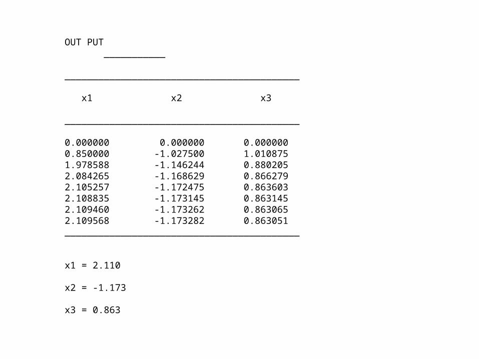
OUT PUT ___________

__________________________________________

x1 x2 x3

__________________________________________

0.000000 0.000000 0.0000000.850000 -1.027500 1.0108751.978588 -1.146244 0.8802052.084265 -1.168629 0.8662792.105257 -1.172475 0.8636032.108835 -1.173145 0.8631452.109460 -1.173262 0.8630652.109568 -1.173282 0.863051__________________________________________

x1 = 2.110

x2 = -1.173

x3 = 0.863

#include<stdio.h>#include<conio.h>#include<math.h>#define e 0.01void main(){ int i,j,k,n; float a[10][10],x[10]; float sum,temp,error,big; printf("Enter the number of equations: "); scanf("%d",&n) ; printf("Enter the coefficients of the equations: \n"); for(i=1;i<=n;i++) { for(j=1;j<=n+1;j++) { printf("a[%d][%d]= ",i,j); scanf("%f",&a[i][j]); } } for(i=1;i<=n;i++) { x[i]=0; } do { big=0; for(i=1;i<=n;i++) {

sum=0; for(j=1;j<=n;j++) { if(j!=i) { sum=sum+a[i][j]*x[j]; } } temp=(a[i][n+1]-sum)/a[i][i]; error=fabs(x[i]-temp); if(error>big) { big=error; } x[i]=temp; printf("\nx[%d] =%f",i,x[i]); }printf("\n"); } while(big>=e); printf("\n\nconverges to solution"); for(i=1;i<=n;i++) { printf("\nx[%d]=%f",i,x[i]); } getch();}

Enter the number of equations: 3Enter the coefficients of the equations:a[1][1]= 2a[1][2]= 1a[1][3]= 1a[1][4]= 5a[2][1]= 3a[2][2]= 5a[2][3]= 2a[2][4]= 15a[3][1]= 2a[3][2]= 1a[3][3]= 4a[3][4]= 8

x[1] =2.500000x[2] =1.500000x[3] =0.375000

x[1] =1.562500x[2] =1.912500x[3] =0.740625

x[1] =1.173437x[2] =1.999688x[3] =0.913359

x[1] =1.043477x[2] =2.008570x[3] =0.976119

x[1] =1.007655x[2] =2.004959x[3] =0.994933

x[1] =1.000054x[2] =2.001995x[3] =0.999474

converges to solutionx[1]=1.000054x[2]=2.001995x[3]=0.999474

1 2 3

1 2 3

1 2 3

2 5

3 5 2 15

2 4 8

x x x

x x x

x x x

1

2

3

1

2

1

x

x

x

Matrix Eigenvalue Problems

In dimensionless form the time–independent Schr¨odinger equation can be written as

The Laplacian,2, can be represented in discrete form as in the case of Laplace’s or Poisson’s equations. For example, in 1D becomes

which can in turn be written in terms of a tridiagonal matrix H as

An alternative and more common procedure is to represent the eigenfunction in terms of a linear combination of basis functions so that we have

(1)

(2)

(3)

(4)

Schrodinger’s equation

2 (r)V Ey y y- Ñ + =

1 1(2 )j j j j jxV Ey d y y y- +- + + - =

H Ey y=

( ) ( )r a rb bb

y f=å

( ) ( )r a rb bb

y f=å

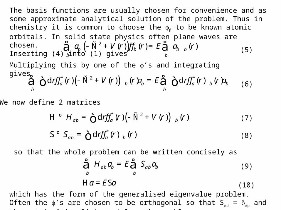
The basis functions are usually chosen for convenience and as some approximate analytical solution of the problem. Thus in chemistry it is common to choose the to be known atomic orbitals. In solid state physics often plane waves are chosen.Inserting (4) into (1) gives

(5)

Multiplying this by one of the ’s and integrating gives

We now define 2 matrices

(6)

(7)

(8)

so that the whole problem can be written concisely as

(9)

(10)which has the form of the generalised eigenvalue problem. Often the ’s are chosen to be orthogonal so that S = and the matrix S is eliminated from the problem.

( )2 ( ) ( ) ( )a V r r E a rb b b bb b

ff- Ñ + =å å

( )* 2 *d ( ) ( ) ( ) d ( ) ( )r r V r r a E r r r aa b b a b bb b

ff ff- Ñ + =å åò ò

( )* 2

*

H d ( ) ( ) ( )

S d ( ) ( )

H r r V r r

S r r r

ab a b

ab a b

ff

ff

º = - Ñ +

º =

òò

H = S

H a E S a

a E a

ab b ab bb b

=å å

In a matrix form,

The eigenvalues are determined by the characteristic equation

General Principles

The usual form of the eigenvalue problem is written

The usual form of the eigenvalue problem is written

where A is a square matrix, x is an eigenvector and is an eigenvalue. Sometimes the eigenvalue and eigenvector are called latent root and latent vector respectively. An N N matrix usually has N distinct eigenvalue/eigenvector pairs. The full solution of the eigenvalue problem can then be written in the form

where is a diagonal matrix of eigenvalues and Ur (Ul) are matrices whose columns (rows) are the corresponding eigenvectors. Ul and Ur are the left and right handed eigenvectors respectively, and Ul = Ur

1.

For Hermitian matrices Ul and Ur are unitary and are therefore Hermitian transposes of each other: Ul + = Ur..

For Real Symmetric matrices Ul and Ur are also real. Real unitary matrices are sometimes called orthogonal.

Ax xa=

AU U

U A Ur r

l l

a

a

=

=

Full Diagonalisation

Routines are available to diagonalise real symmetric, Hermitian, tridiagonal and general matrices.

In the first 2 cases this is usually a 2 step process in which the matrix is first tridiagonalised (transformed to tridiagonal form) and then passed to a routine for diagonalising a tridiagonal matrix. Routines are available which find only the eigenvalues or both eigenvalues and eigenvectors. The former are usuallymuch faster than the latter.

Usually the eigenvalues of a Hermitian matrix are returned sorted into ascending order, but this is not always the case (check the description of the routine). Also the eigenvectors are usually normalised to unity.

For non–Hermitian matrices only the right–handed eigenvectors are returned and are not normalised.

The Generalised Eigenvalue Problem

A common generalisation of the simple eigenvalue problem involves 2 matrices

This can easily be transformed into a simple eigenvalue problem by multiplying both sides by the inverse of either A or B. This has the disadvantage however that if both matrices are Hermitian B1A is not, and the advantages of the symmetry are lost, together, possibly, with some important physics. There is actually a more efficient way of handling the transformation. Using Cholesky factorisation an LU decomposition of a positive definite matrix can be carried out such that

which can be interpreted as a sort of square root of B. Using this we can transform the problem into the form

A Bx xa=

†B LL=

1 † 1 † †L A (L ) L L

A '

x x

y y

a

a

- -é ùé ù é ù=ê úê ú ê úë ûë û ë û

=

Cholesky factorization algorithm

Partition matrices in A = LLT as

algorithm

1. determine l11 and L21:

2. compute L22 from

this is a Cholesky factorization of order n − 1.

1111 21 11 21

21 2221 22 22

0

0

T T

T

la A l L

L LA A L

é ù é ùé ùê ú ê úê ú=ê ú ê úê úë ûë û ë û

211 11 21

11 21 21 21 22 22

T

T T

l l L

l L L L L L

é ùê ú= ê ú+ë û

11 11 21 2111

1 l a L A

l= =

22 21 21 22 22T TA L L L L- =

Example: Cholesky factorization

11 11 12 31

21 22 22 32

31 32 33 33

25 15 5 0 0

15 18 0 0 0

5 0 11 0 0

l l l l

l l l l

l l l l

é ù é ùé ùê ú ê úê úê ú ê úê ú=ê ú ê úê úê ú ê úê ú-ë û ë ûë û

211 11 12 11 31

221 11 21 12 22 21 13 22 23

231 11 31 12 32 22 31 13 32 23 33

25 15 5

15 18 0

5 0 11

l l l l l

l l l l l l l l l

l l l l l l l l l l l

é ùé ù ê úê úê úê ú= + +ê úê úê úê ú- + + +ê úë û ë û

( )( )( )( ) ( )( )( )

211 11

11 12 12

11 13 13

21 11 21

31 11 31

2 221 12 22 22 22

31 12 32 22 32 32

21 13 22 23

25, 5

15 3

5 1

15 3

5 1

18 3 3 18 3

0 1 3 3 0 1

0 3 1

l l

l l l

l l l

l l l

l l l

l l l l l

l l l l l l

l l l l

= =

= =

= =

= =

=- =-

+ = + = =

+ = - + = =

+ = +( )

( )( ) ( )( )23 23

2 231 13 32 23 33 33 33

3 0 1

2 1 1 1 1 2 2

l l

l l l l l l l

= =-

+ + = - + - + = =

Third column of L: 10 - 1 = l233, i.e., l33 = 3 second column of Lconclusion:

second column of L

First column of L

22 22 32

32 33 33

25 15 5 5 0 0 5 3 1

15 18 0 3 0 0

5 0 11 1 0 0

l l l

l l l

é ù é ùé ù-ê ú ê úê úê ú ê úê ú=ê ú ê úê úê ú ê úê ú-ë û ë ûë û

[ ] 22 22 32

32 33 33

018 0 33 1

00 11 1

l l l

l l l

é ùé ùé ù é ùê úê úê ú ê ú- - = ê úê úê ú ê ú-ë û ë û ë ûë û

33 33

3 0 3 19 3

1 03 10 l l

é ùé ùé ùê úê úê ú= ê úê úê úë û ë ûë û

25 15 5 5 0 0 5 3 1

15 18 0 3 3 0 0 3 1

5 0 11 1 1 3 0 0 3

é ù é ùé ù-ê ú ê úê úê ú ê úê ú=ê ú ê úê úê ú ê úê ú- -ë û ë ûë û

Here is the Cholesky decomposition of a symmetric real matrix:

And here is the LDLT decomposition of the same matrix:

4 12 16 2 2 6 8

12 37 43 6 1 1 5

16 43 98 8 5 3 3

é ù é ùé ù- -ê ú ê úê úê ú ê úê ú- =ê ú ê úê úê ú ê úê ú- - -ë û ë ûë û

4 12 16 1 4 1 3 4

12 37 43 3 1 1 1 5

16 43 98 4 5 1 9 1

é ù é ùé ùé ù- -ê ú ê úê úê úê ú ê úê úê ú- =ê ú ê úê úê úê ú ê úê úê ú- - -ë û ë ûë ûë û

11 12 13 11 11 11 12 13

21 22 23 21 22 22 22 23

31 32 33 31 32 33 33 33

0 0 0 0

0 0 0 0

0 0 0 0

M M M a b c c c

M M M a a b c c

M M M a a a b c

é ù é ùé ùé ùê ú ê úê úê úê ú ê úê úê ú=ê ú ê úê úê úê ú ê úê úê úë û ë ûë ûë û

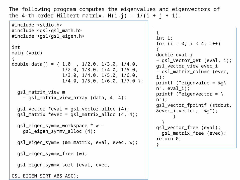
#include <stdio.h>#include <gsl/gsl_math.h>#include <gsl/gsl_eigen.h>

intmain (void){double data[] = { 1.0 , 1/2.0, 1/3.0, 1/4.0, 1/2.0, 1/3.0, 1/4.0, 1/5.0, 1/3.0, 1/4.0, 1/5.0, 1/6.0, 1/4.0, 1/5.0, 1/6.0, 1/7.0 };

gsl_matrix_view m = gsl_matrix_view_array (data, 4, 4);

gsl_vector *eval = gsl_vector_alloc (4); gsl_matrix *evec = gsl_matrix_alloc (4, 4);

gsl_eigen_symmv_workspace * w = gsl_eigen_symmv_alloc (4); gsl_eigen_symmv (&m.matrix, eval, evec, w);

gsl_eigen_symmv_free (w);

gsl_eigen_symmv_sort (eval, evec, GSL_EIGEN_SORT_ABS_ASC);

The following program computes the eigenvalues and eigenvectors of the 4-th order Hilbert matrix, H(i,j) = 1/(i + j + 1).

{int i;for (i = 0; i < 4; i++){double eval_i = gsl_vector_get (eval, i);gsl_vector_view evec_i = gsl_matrix_column (evec, i);printf ("eigenvalue = %g\n", eval_i);printf ("eigenvector = \n");gsl_vector_fprintf (stdout, &evec_i.vector, "%g"); } }gsl_vector_free (eval); gsl_matrix_free (evec);return 0;}

#include <stdlib.h>#include <stdio.h>

/* DSYEV prototype */extern void dsyev( char* jobz, char* uplo, int* n, double* a, int* lda,                double* w, double* work, int* lwork, int* info );/* Auxiliary routines prototypes */extern void print_matrix( char* desc, int m, int n, double* a, int lda );

/* Parameters */#define N 5#define LDA N

/* Main program */int main() {        /* Locals */        int n = N, lda = LDA, info, lwork;        double wkopt;        double* work;        /* Local arrays */        double w[N];        double a[LDA*N] = {            1.96,  0.00,  0.00,  0.00,  0.00,           -6.49,  3.80,  0.00,  0.00,  0.00,           -0.47, -6.39,  4.17,  0.00,  0.00,           -7.20,  1.50, -1.51,  5.70,  0.00,           -0.65, -6.34,  2.67,  1.80, -7.10        };        /* Executable statements */        printf( " DSYEV Example Program Results\n" );

   DSYEV Example.

        /* Query and allocate the optimal workspace */        lwork = -1;        dsyev( "Vectors", "Upper", &n, a, &lda, w, &wkopt, &lwork, &info );        lwork = (int)wkopt;        work = (double*)malloc( lwork*sizeof(double) );        /* Solve eigenproblem */        dsyev( "Vectors", "Upper", &n, a, &lda, w, work, &lwork, &info );        /* Check for convergence */        if( info > 0 ) {                printf( "The algorithm failed to compute eigenvalues.\n" );                exit( 1 );        }        /* Print eigenvalues */        print_matrix( "Eigenvalues", 1, n, w, 1 );        /* Print eigenvectors */        print_matrix( "Eigenvectors (stored columnwise)", n, n, a, lda );        /* Free workspace */        free( (void*)work );        exit( 0 );} /* End of DSYEV Example */

/* Auxiliary routine: printing a matrix */void print_matrix( char* desc, int m, int n, double* a, int lda ) {        int i, j;        printf( "\n %s\n", desc );        for( i = 0; i < m; i++ ) {                for( j = 0; j < n; j++ ) printf( " %6.2f", a[i+j*lda] );                printf( "\n" );        }}

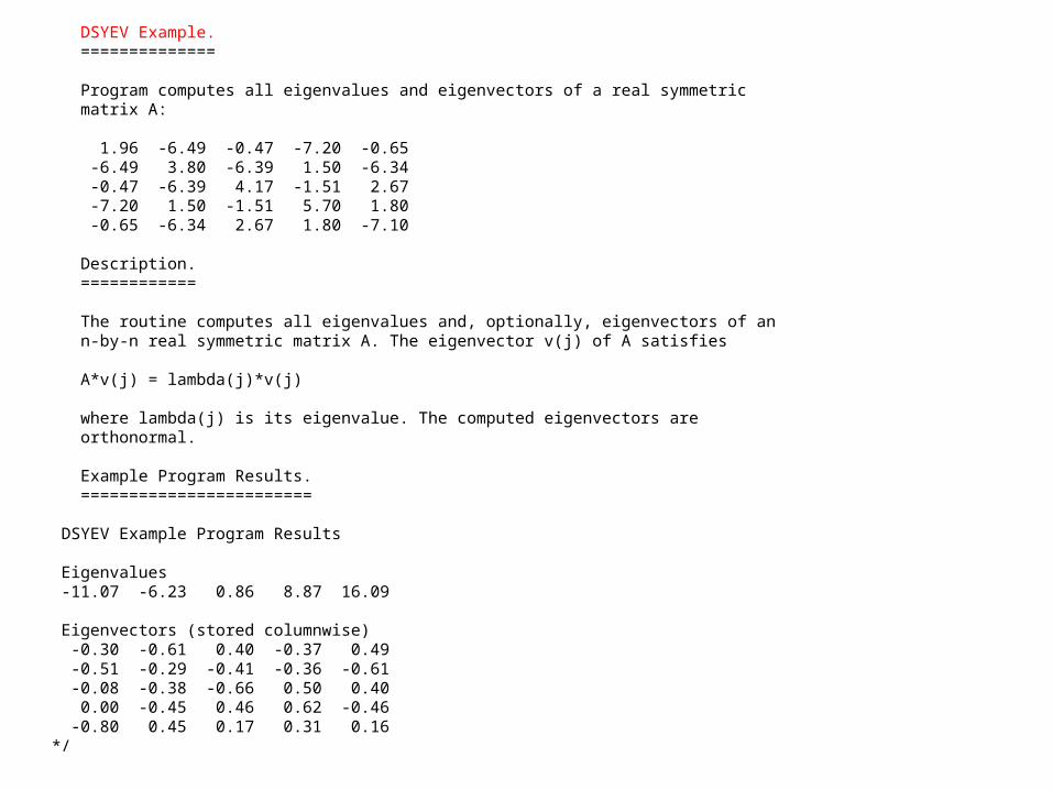
   DSYEV Example.   ==============

   Program computes all eigenvalues and eigenvectors of a real symmetric   matrix A:

     1.96  -6.49  -0.47  -7.20  -0.65    -6.49   3.80  -6.39   1.50  -6.34    -0.47  -6.39   4.17  -1.51   2.67    -7.20   1.50  -1.51   5.70   1.80    -0.65  -6.34   2.67   1.80  -7.10

   Description.   ============

   The routine computes all eigenvalues and, optionally, eigenvectors of an   n-by-n real symmetric matrix A. The eigenvector v(j) of A satisfies

   A*v(j) = lambda(j)*v(j)

   where lambda(j) is its eigenvalue. The computed eigenvectors are   orthonormal.

   Example Program Results.   ========================

 DSYEV Example Program Results

 Eigenvalues -11.07  -6.23   0.86   8.87  16.09

 Eigenvectors (stored columnwise)  -0.30  -0.61   0.40  -0.37   0.49  -0.51  -0.29  -0.41  -0.36  -0.61  -0.08  -0.38  -0.66   0.50   0.40   0.00  -0.45   0.46   0.62  -0.46  -0.80   0.45   0.17   0.31   0.16*/

W Kinzel_Physics by Computer (using Mathematica and C)

Monte Carlo simulation

http://www.cmth.ph.ic.ac.uk/people/a.mackinnon/Lectures/cp3/node54.html

http://oregonstate.edu/instruct/ch590/lessons/lesson13.htm