Computational Learning Theory;The Tradeoff between

Computational Complexityand Statistical Soundness

Computational Learning Theory;The Tradeoff between

Computational Complexityand Statistical Soundness

Shai Ben-David

CS Department, Cornell

and

Technion, Haifa, Israel

IntroductionIntroductionThe complexity of leaning is measured mainly along

two axis:: Information Information and computationcomputation..

Information complexityInformation complexity is concerned with the generalization performance of learning; How many training examples are needed? How fast do learner’s estimate converge to the true population

parameters? Etc. The Computational complexity Computational complexity concerns the computation applied to the

training data to extract from it learner’s predictions.

It seems that when an algorithm improves with respect to one of these measures it deteriorates with respect to the other.

Outline of this TalkOutline of this Talk

1. Some background.

2. Survey of recent pessimistic computational

hardness results .

3. A discussion of three different directions for solutions:

a. The Support Vector Machines approach.

b. The Boosting approach (an agnostic learning variant).

c. Algorithms that are efficient for `well behaved’ inputs.

The Label Prediction ProblemThe Label Prediction Problem

Given some domainset XX

A sample SS of labeledmembers of XX is generated by some(unknown) distribution

For a next point xx , predict its label

Files of personal data of (car) drivers.

Will the current driverundergo an accident?

Files in a sample are labeled according to driver’s involvement in car accident.

Formal Definition Example

Empirical Risk Minimization Paradigm

Empirical Risk Minimization Paradigm

Choose a Hypothesis Class HH of subsets of XX.

For an input sample SS , find some hh in HH that fits SS well.

For a new point x , predict a label according to its membership in hh .

The Mathematical JustificationThe Mathematical Justification

Assume both a training sample SS and the test point (x,l)(x,l)

are generated by the same distribution over X x {0,1}X x {0,1} then,

If HH is not too rich (e.g., has small VC-dimension), for every hh in HH ,

the empirical success ratio of hh on the sample SS

is a good estimate of its probability of success on the new xx .

Two Basic Competing ModelsTwo Basic Competing Models

Sample labels are consistentwith some hh in HH

Learner’s hypothesis required to meet absolute upper boundon its error

No prior restriction on the sample labels

The required upper bound on the hypothesis error is only relative (to the best hypothesis in the class)

PAC framework Agnostic framework

The Types of Errors to be ConsideredThe Types of Errors to be Considered

Best regressor for DD

Approximation ErrorEstimation Error

}Hh:)h(Ermin{Arg

}Hh:)h(srEmin{Arg

The Class H

The Computational ProblemThe Computational Problem

Given a class HH of subsets of RRnn

Input:: A finite set of {0, 1}{0, 1}-labeled

points SS in RRnn .

Output:: Some ‘hypothesis’ function h in H H that

maximizes the number of correctly classified

points of S .

The Types of Errors to be ConsideredThe Types of Errors to be Considered

Output of the the learning Algorithm

Best regressor for DD

Approximation ErrorEstimation Error

Computational Error

}Hh:)h(Ermin{Arg

}Hh:)h(srEmin{Arg

The Class H

For each of the following classes, approximating the

best agreement rate for h in HH (on a given input

sample SS ) up to some constant ratio, is NP-hard :Monomials Constant widthMonotone Monomials

Half-spacesHalf-spaces Balls Axis aligned RectanglesThreshold NN’s with constant 1st-layer width

BD-Eiron-Long

Bartlett- BD

Hardness-of-Approximation ResultsHardness-of-Approximation Results

Gaps in Our KnowledgeGaps in Our Knowledge

The additive constants in the hardness-

of-approximation results are 1%-2%.1%-2%.

They do not rule out efficient algorithms

achieving, say, 90%(optimal success rate).

However, currently, there are no efficient

algorithm whose success-rate guarantees are

significantly above 50%.

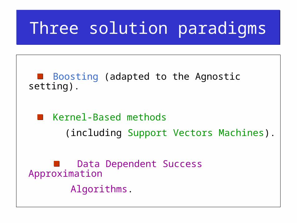
Three solution paradigmsThree solution paradigms

Boosting (adapted to the Agnostic setting).

Kernel-Based methods

(including Support Vectors Machines).

Data Dependent Success Approximation

Algorithms.

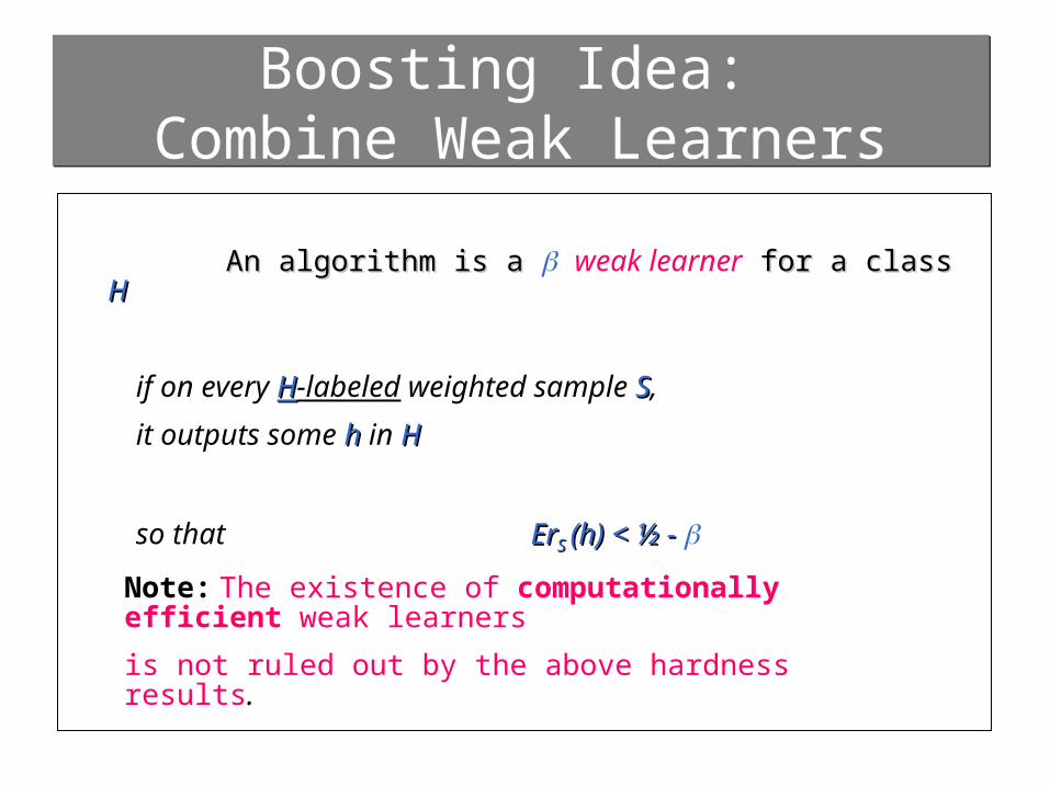
:Boosting IdeaCombine Weak Learners

Boosting Idea:Combine Weak Learners

An algorithm is a An algorithm is a weak learner for a class for a class HH

if on every HH-labeled weighted sample SS,

it outputs some hh in HH

so that ErErS S (h) < ½ - (h) < ½ -

Note: The existence of computationally efficient weak learners

is not ruled out by the above hardness results.

Boosting Solution: the Basic Result Boosting Solution: the Basic Result

[Schapire ’89, Freund ’90] [Schapire ’89, Freund ’90]

Having access to a computationally efficient weak

learner,

for a PP -random HH -sample SS, and parameters , ,

the boosting algorithm efficiently finds some hh in Co(H)Co(H)

so that

ErErP P (h) < (h) < ,with prob. .

Note: Since hh may be outside HH, there is no conflict

with the computational hardness results.

The Boosting Solution in PracticeThe Boosting Solution in Practice

The boosting approach was embraced by The boosting approach was embraced by

practitioners of Machine Learning and applied,practitioners of Machine Learning and applied,

quite successfully, to a wide variety of real-lifequite successfully, to a wide variety of real-life

problems.problems.

Theoretical Problems with the The Boosting Solution

Theoretical Problems with the The Boosting Solution

The boosting results assume that the input sampleThe boosting results assume that the input sample

labeling is consistent with some function in Hlabeling is consistent with some function in H

(the PAC framework assumption).(the PAC framework assumption).

In practice this is never the caseIn practice this is never the case..

The boosting algorithm’s success is based on havingThe boosting algorithm’s success is based on having

access to an efficient weak learner – access to an efficient weak learner –

for most classesfor most classes, , no such learner is known to existno such learner is known to exist..

Attempt to Recover Boosting TheoryAttempt to Recover Boosting Theory

Can one settle for weaker, realistic, assumptions?Can one settle for weaker, realistic, assumptions?

Agnostic weak learners :Agnostic weak learners :

an algorithm is a weak agnostic learner for HH,

if for every labeled sample SS it finds hh in HH s.t.

ErErS S (h) < Er(h) < ErS S (Opt(H)) + (Opt(H)) +

Agnostic weak learners always exist

Revised Boosting SolutionRevised Boosting Solution

[B-D, Long, Mansour (2001)] [B-D, Long, Mansour (2001)]

There is a computationally efficient algorithm that,

having access to a weak agnostic learner,

finds h h in Co(H)Co(H) s.t.

ErErP P (h) < c Er(h) < c ErP P (Opt(H))(Opt(H))c’c’

(Where c c and c’c’ are constants depending only on )

The SVM ParadigmThe SVM Paradigm

Choose an Embedding of the domain X X into

some high dimensional Euclidean space,

so that the data sample becomes (almost)

linearly separable.

Find a large-margin data-separating hyperplane

in this image space, and use it for prediction.

Important gain: When the data is separable,

finding such a hyperplane is computationally feasible.

The SVM Idea: an ExampleThe SVM Idea: an Example

The SVM Idea: an ExampleThe SVM Idea: an Example

The SVM Idea: an ExampleThe SVM Idea: an Example

The SVM Solution in PracticeThe SVM Solution in Practice

The SVM approach is embraced by The SVM approach is embraced by

practitioners of Machine Learning and applied,practitioners of Machine Learning and applied,

very successfully, to a wide variety of real-lifevery successfully, to a wide variety of real-life

problems.problems.

A Potential Problem: GeneralizationA Potential Problem: Generalization

VC-dimension boundsVC-dimension bounds:: The VC-dimension of

the class of half-spaces in RRnn is n+1 n+1.

Can we guarantee low dimension of the embeddings range?

Margin boundsMargin bounds: : Regardless of the Euclidean dimension, ,

ggeneralization can bounded as a function of the margins

of the hypothesis hyperplane.

Can one guarantee the existence of a large-margin separation?

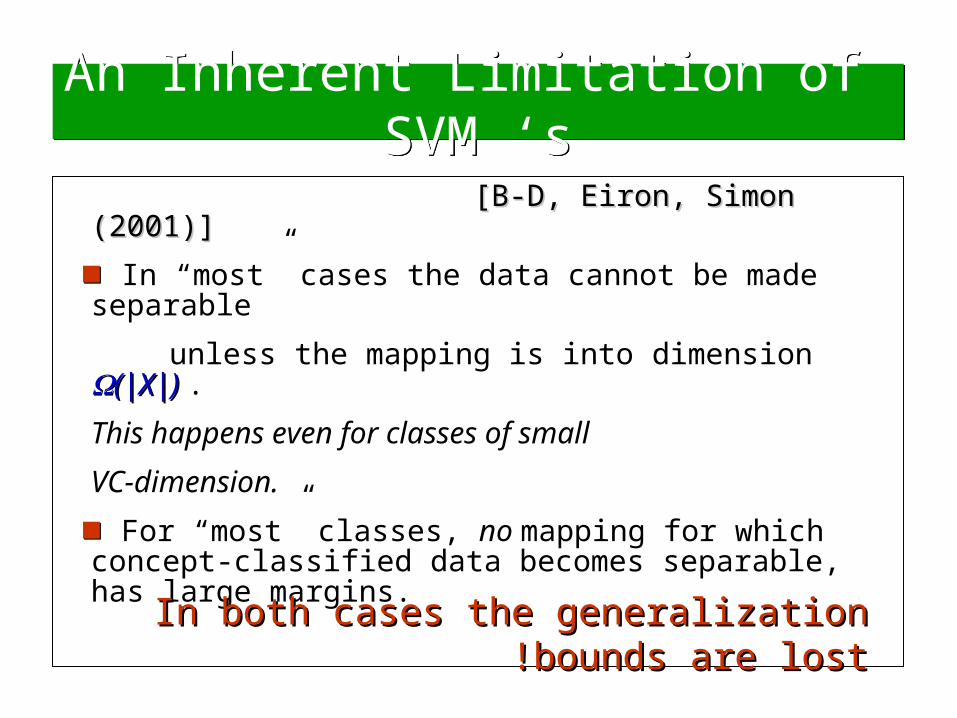
An Inherent Limitation of SVM ‘sAn Inherent Limitation of SVM ‘s

[B-D, Eiron, Simon (2001)] [B-D, Eiron, Simon (2001)]

In “most” cases the data cannot be made separable

unless the mapping is into dimension (|X|) (|X|) .

This happens even for classes of small

VC-dimension.

For “most” classes, no mapping for which concept-classified data becomes separable, has large margins.

In both cases the generalization bounds are lostIn both cases the generalization bounds are lost!!

A Proposal for a Third Solution:Data-Dependent Success Approximations

A Proposal for a Third Solution:Data-Dependent Success Approximations

With an eye on the gap between the theoretical hardness-of-approximation results and the experimental success of practical learning algorithms,

we propose a new measure of the quality of an approximation algorithm

Data Dependent Approximation:

The required success-rate is a function of the input data.

Data Dependent Success Definition for Half-spaces

Data Dependent Success Definition for Half-spaces

A learning algorithm AA is

marginsuccessful

if, for every input S S R Rnn {0,1} {0,1} ,

|{(x,y) S: A(s)(x) = y}| > |{(x,y): h(x)=y and d(h, x) >

for every half-space hh.

Classifying with MarginsClassifying with Margins

Some IntuitionSome Intuition

If there exist some optimal h which separates with generous margins, then a margin

algorithm must produce an optimal separator.

On the other hand,

If every good separator can be degraded by small perturbations, then a margin algorithm can settle for a hypothesis that is far from optimal.

Main Positive Result Main Positive Result

For every positive , there is an efficient margin algorithm.

That is, the algorithm that classifies correctly as many input points as any half-space can classify correctly with margin

A Crisp Threshold PhenomenaA Crisp Threshold Phenomena

The positive result

For every positive there is a - margin nonsealgorithm whose running time is polynomial stam in |S|S| and nn .

A Complementing Hardness Result

Unless P = NP , no algorithm can do this in timeblablaaaaaaaaaaaaaaaaaaaaaaaaaa aaaaaa aaaaaatime polynomial in and in |S||S| and nn ).

Some Obvious Open QuestionsSome Obvious Open Questions

Is there a parameter that can be

used to ensure good generalization for

Kernel –Based (SVM-like) methods?

Are there efficient Agnostic Weak Learners

for potent hypothesis classes?

Is there an inherent trade-off between

the generalization ability and the computational

complexity of algorithms?

THE END