Computational Electronics

Generalized Monte Carlo Tool for Investigating Low-Field and High Field

Properties of Materials Using Non-parabolic Band Structure Model

Raghuraj Hathwar

Advisor : Dr. Dragica Vasileska

Computational Electronics

Outline

• Motivation of modeling different materials

- Strained Silicon

- III-V and II-VI materials

- Silicon Carbide

• The generalized Monte Carlo code

- Free-Flight and drift velocity calculation

• Rappture interfacing

• Results

• Conclusions and future work.

Computational Electronics

Technology Trends

Computational Electronics

Strained Silicon

• The four minima of the conduction band in directions parallel to the plane of strain are raised. This results in higher electron mobility.

• There is also a splitting of the light and heavy hole bands leading to increased hole mobility.

Computational Electronics

Substrate

Barrier / buffer

Channel layer

Drain

BarrierL

n+ cap

Gate

n+ cap

2DEG channel

Source

III-V and II-VI Materials

• High electron mobility of compared to silicon.

• AlGaAs/GaAs are lattice matched.

• AlGaN/GaN interfaces have spontaneous polarization.

Computational Electronics

Silicon Carbide (SiC)

• Very useful in high voltage devices because of its thermal conductivity, high band gap and high breakdown field.

• In fact the thermal conductivity of 4H-SiC is greater than that of copper at room temperature.

Computational Electronics

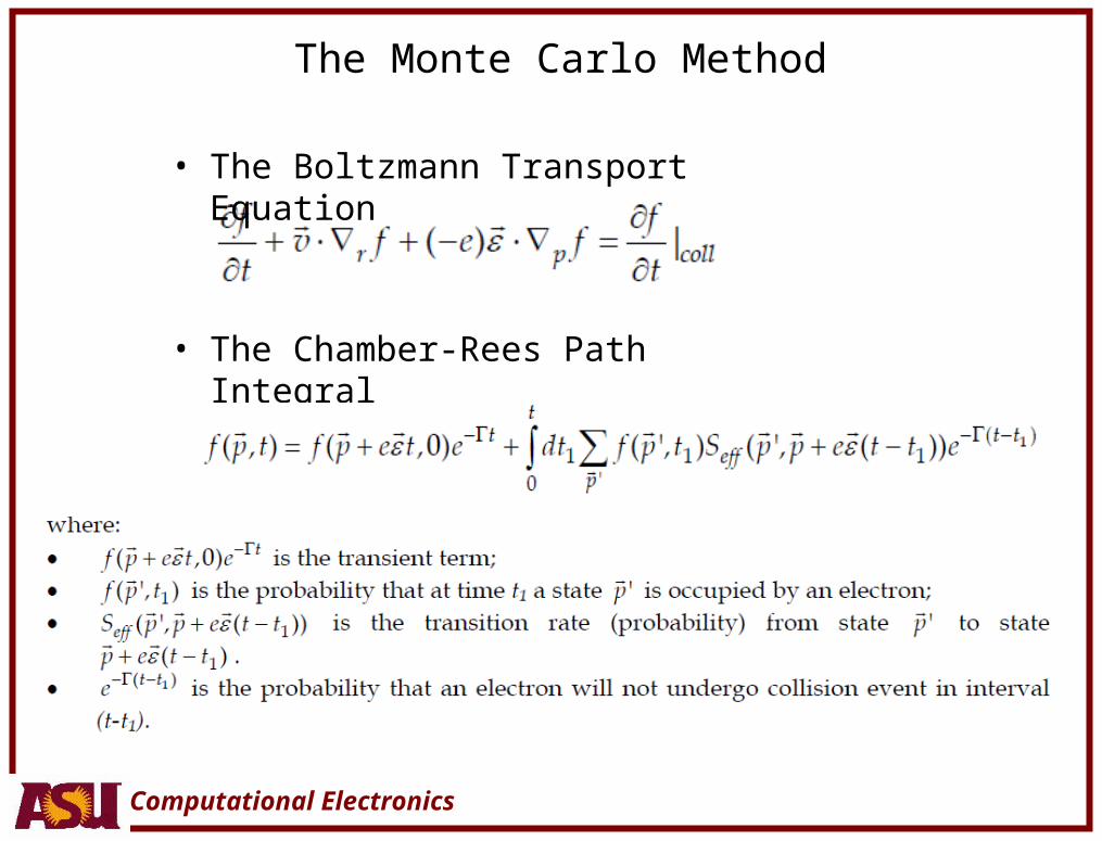
• The Boltzmann Transport Equation

• The Chamber-Rees Path Integral

The Monte Carlo Method

Computational Electronics

The Generalized Monte Carlo Flow Chart

Computational Electronics

Types of Scattering

• Acoustic Phonon Scattering

• Zeroth order Intervalley Scattering

• First order Intervalley Scattering

• Piezoelectric Scattering

• Polar Optical Phonon Scattering

• Ionized Impurity Scattering

Computational Electronics

Fermi’s Golden Rule and Scattering Rates Calculation

• Calculate the Matrix Element

• Use Fermi’s Golden Rule

• Sum over all k’ states

Computational Electronics

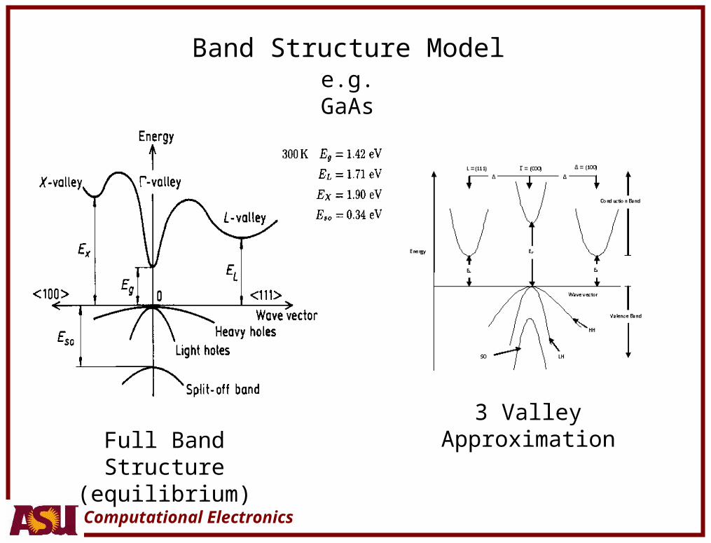
Band Structure Model e.g. GaAs

Full Band Structure(equilibrium)

3 Valley Approximation

Computational Electronics

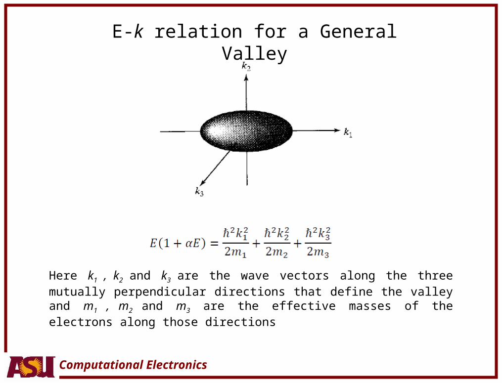
E-k relation for a General Valley

Here k1 , k2 and k3 are the wave vectors along the three mutually perpendicular directions that define the valley and m1 , m2 and m3 are the effective masses of the electrons along those directions

Computational Electronics

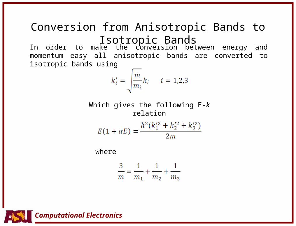
Conversion from Anisotropic Bands to Isotropic Bands

In order to make the conversion between energy and momentum easy all anisotropic bands are converted to isotropic bands using

Which gives the following E-k relation

where

Computational Electronics

Carrier Free-Flight

From Newton’s 2nd law and Q.M.

Computational Electronics

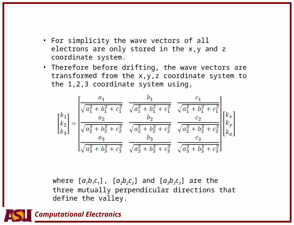
• For simplicity the wave vectors of all electrons are only stored in the x,y and z coordinate system.

• Therefore before drifting, the wave vectors are transformed from the x,y,z coordinate system to the 1,2,3 coordinate system using,

where [a1b1c1], [a2b2c2] and [a3b3c3] are the three mutually perpendicular directions that define the valley.

Computational Electronics

• The electric fields must also be transformed to the directions along the wave vectors

• The electrons are then drifted and transformed back into the x,y,z coordinate system.

Computational Electronics

Drift Velocity Calculation

Computational Electronics

The drift velocities must then be transformed to the x,y,z coordinate system so that an average can be taken over all electrons.

Computational Electronics

Rappture Integration

• The Rappture toolkit provides the basic infrastructure for a large class of scientific applications, letting scientists focus on their core algorithm when developing new simulators.

• Instead of inventing your own input/output, you declare the parameters associated with your tool by describing Rappture objects in the Extensible Markup Language (XML).

• Create an xml file describing the input structure.

• Integrate the source code with Rappture to read input values and to output results to the Rappture GUI.

Computational Electronics

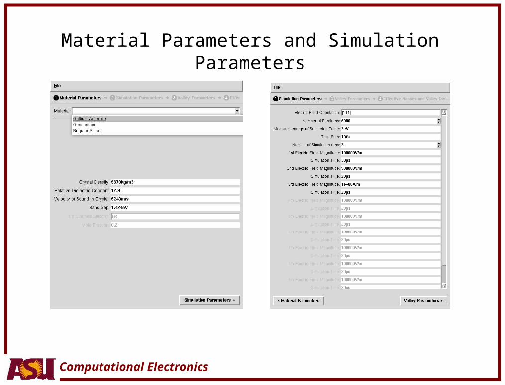
Material Parameters and Simulation Parameters

Computational Electronics

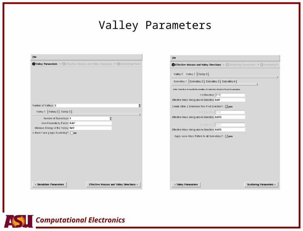
Valley Parameters

Computational Electronics

Scattering Parameters

Computational Electronics

Drift Velocity vs Electric Field Electron Energy vs Electric Field

Silicon

Computational Electronics

Gallium Arsenide (GaAs)

Drift Velocity vs Electric Field Electron Energy vs Electric Field

Computational Electronics

Fraction of electrons in the L valley vs Electric Field

Computational Electronics

Drift Velocity vs Electric Field Electron Energy vs Electric Field

Germanium (Ge)

Computational Electronics

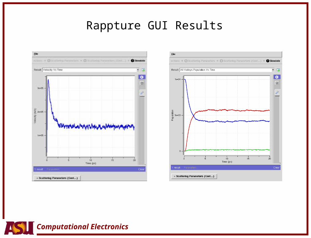
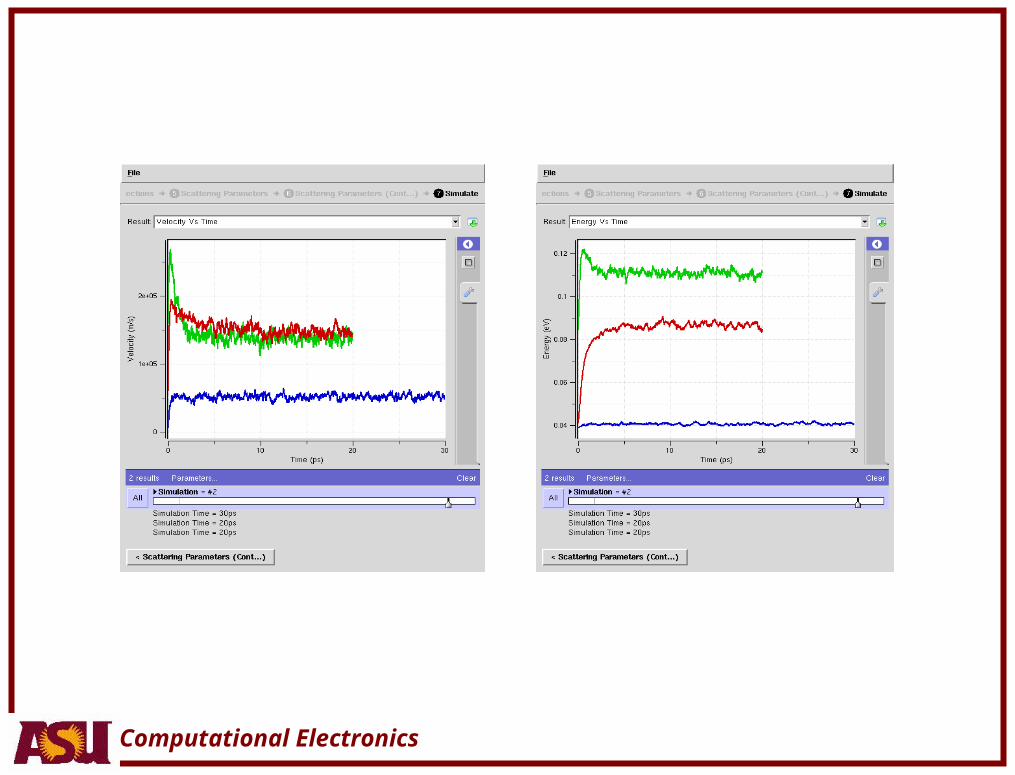
Rappture GUI Results

Computational Electronics

Computational Electronics

Conclusions and Future Work

• Uses non-parabolic band structure making it as accurate as possible for an analytic representation of the band structure.

• Interfacing the tool with Rappture enables easy handling of the parameters and reduces the complexity of using the tool.

• Existing materials band structures can be easily modified to improve existing results.

• New materials can easily be added to the code.

• The tool can be extended to include impact ionization scattering to better model high field properties.

• Full band simulation for holes.