COMPUTATIONAL COMPLEXITY ANALYSIS FOR MONTE CARLO ...

MULTISCALE MODEL. SIMUL. c© 2018 Society for Industrial and Applied MathematicsVol. 16, No. 3, pp. 1206–1226

COMPUTATIONAL COMPLEXITY ANALYSIS FOR MONTECARLO APPROXIMATIONS OF CLASSICALLY SCALED

POPULATION PROCESSES∗

DAVID F. ANDERSON† , DESMOND J. HIGHAM‡ , AND YU SUN§

Abstract. We analyze and compare the computational complexity of different simulation strate-gies for Monte Carlo in the setting of classically scaled population processes. This allows a rangeof widely used competing strategies to be judged systematically. Our setting includes stochasticallymodeled biochemical systems. We consider the task of approximating the expected value of somepath functional of the state of the system at a fixed time point. We study the use of standard MonteCarlo when samples are produced by exact simulation and by approximation with tau-leaping or anEuler–Maruyama discretization of a diffusion approximation. Appropriate modifications of recentlyproposed multilevel Monte Carlo algorithms are also studied for the tau-leaping and Euler–Maruyamaapproaches. In order to quantify computational complexity in a tractable yet meaningful manner,we consider a parameterization that, in the mass action chemical kinetics setting, corresponds to theclassical system size scaling. We base the analysis on a novel asymptotic regime where the requiredaccuracy is a function of the model scaling parameter. Our new analysis shows that, under thespecific assumptions made in the manuscript, if the bias inherent in the diffusion approximation issmaller than the required accuracy, then multilevel Monte Carlo for the diffusion approximation ismost efficient, besting multilevel Monte Carlo with tau-leaping by a factor of a logarithm of thescaling parameter. However, if the bias of the diffusion model is greater than the error tolerance orif the bias cannot be bounded analytically, multilevel versions of tau-leaping are often the optimalchoice.

Key words. computational complexity, variance, reaction networks, classical scaling, coupling,multilevel Monte Carlo

AMS subject classifications. 60H35, 65C05, 92C40

DOI. 10.1137/17M1138169

1. Introduction. For some large N0 > 0, we consider a continuous time Markovchain satisfying the stochastic equation

XN0(t) = XN0(0) +

K∑k=1

1

N0Yk

(N0

∫ t

0

λk(XN0(s))ds

)ζk,(1)

where XN0(t) ∈ Rd, K <∞, the Yk are independent unit Poisson processes, and, foreach k, ζk ∈ Rd and λk : Rd → R≥0 satisfies mild regularity conditions. For a givenpath functional f , we consider the task of numerically approximating E[f(XN0(·))],in the sense of confidence intervals, to some fixed tolerance ε0 < 1. Specifically,we consider the computational complexity, as quantified by the number of random

∗Received by the editors July 12, 2017; accepted for publication (in revised form) May 30, 2018;published electronically August 7, 2018.

http://www.siam.org/journals/mms/16-3/M113816.htmlFunding: The first author was supported by grant support from NSF-DMS-1318832 and Army

Research Office W911NF-14-1-0401. The second author was supported by grant support from a Wolf-son/Royal Society Research Merit Award and an EPSRC Fellowship with reference EP/M00158X/1.EPSRC data statement: Not relevant.†Department of Mathematics, University of Wisconsin, Madison, WI 53706 (anderson@math.

wisc.edu).‡Department of Mathematics and Statistics, University of Strathclyde, UK (d.j.higham@maths.

strath.ac.uk).§Facebook, Inc., 1 Hacker Way, Menlo Park, CA 94025 ([email protected]).

1206

http://www.siam.org/journals/mms/16-3/M113816.html

mailto:[email protected]





MONTE CARLO FOR CLASSICALLY SCALED PROCESSES 1207

variables utilized, required by different Monte Carlo schemes to achieve a root meansquared error of ε0. For concreteness, we will assume throughout that the pathfunctional f depends upon XN0(·) only on the compact time interval [0, T ].

The class of models of the form (1) has a long history in terms of modeling[12, 13, 14, 31], analysis [9, 27, 28], and computation [18, 19]. The framework coversmany application areas, including population dynamics [32], queueing theory [33], andseveral branches of physics [15]. In recent years, chemical and biochemical kineticsmodels in systems biology [34] have been the driving force behind a resurgence ofactivity in algorithmic developments, including tau-leaping [20] and its multilevelextension [4, 5]. In this setting, the parameter N0 in (1) can represent Avogadro’snumber multiplied by the volume, and in this classical scaling, species are measuredin moles per liter. More generally, however, N0 can just be considered a large number,often of the order 100s or 1000s.

In section 2, we discuss some of the issues involved in quantifying computationalcomplexity in the present setting, and introduce a novel scaling regime in which clear-cut comparisons can be made. Further, the specific assumptions utilized throughoutthe manuscript are presented, and a high-level summary of our main conclusionsis presented. In section 3, we summarize two widely used approximation methodsfor the model (1): the tau-leap discretization method and the Langevin or diffusionapproximation. In section 4, we quantify the computational complexity of using exactsimulation, tau-leaping, and simulation of the diffusion equation with standard MonteCarlo for approximating E[f(XN0(·))] to a desired tolerance under our assumptions.Further, in subsection 4.2, we review the more recent multilevel methods and quantifythe benefits of their use in both the tau-leaping and the diffusion scenarios. In section5, we provide numerical examples demonstrating our main conclusions. In section 6,we close with some brief conclusions.

This paper makes use of results from two recent papers:• In [5], an analysis was carried out to determine the variance of the difference

between coupled paths in the jump process setting under a more generalscaling than is considered here.

• In [6], an analysis was carried out to determine the variance of the differencebetween coupled paths in the setting of stochastic differential equations withsmall noise.

Our goals here are distinct from those of these two papers. First, the analysis in [5]allowed such a general scaling that no modified versions of Euler-based tau-leaping,such as midpoint or trapezoidal tau-leaping, could be considered. Here, we consider aparticular scaling (which is the most common in the literature) and present a unifiedcomputational complexity analysis for a range of Monte Carlo–based methods. Thisallows us to make what we believe are the first concrete conclusions pertaining to therelative merits of current methods in a practically relevant asymptotic regime. More-over, an open question in the literature involves the selection of the finest time stepin the unbiased version of multilevel Monte Carlo (since it is not constrained by theaccuracy requirement). By carrying out our analysis in this particular scaling regime,we are able to determine the asymptotics for the optimal selection of this parameter.Selecting the finest time step according to this procedure is shown to lower the com-putational complexity of the method by a nontrivial factor. See the end of section4.2.2 for this derivation and the end of section 5 for a numerical example. Second,it has become part of the “folk wisdom” surrounding these models that in the par-ticular scaling considered here, properly implemented numerical methods applied tothe diffusion approximation are the best choice. This idea was somewhat exacerbated

1208 DAVID F. ANDERSON, DESMOND J. HIGHAM, AND YU SUN

by the analysis in [6], which applied to a key aspect of the algorithm. There it wasshown that the variance between the coupled paths of a diffusion approximation isasymptotically smaller than the variance between the properly scaled jump processes.However, here we show that the actual difference in overall complexity between prop-erly implemented versions of multilevel Monte Carlo for the diffusion approximationand for the jump process never differ by more than a logarithm term. If one combinesthis conclusion with the fact that the bias of the diffusion approximation itself is oftenunknown, whereas multilevel Monte Carlo applied to the jump process is naturallyunbiased, then the folk wisdom is overturned and unbiased multilevel Monte Carlo isseen as a competitive choice.

2. Scaling, assumptions, and a summary of results. In order to motivateour analysis and computations, we begin with a brief high-level overview. In partic-ular, we discuss the entries in Table 1, which summarizes the key conclusions of thiswork. Full details are given later in the manuscript; however, we point out here thatthe terms in Table 1 include assumptions on the variances of the constituent processesthat will be detailed below.

A natural approach to approximate the desired expectation is to simulate pathsexactly, for example, with the stochastic simulation algorithm [18, 19] or the nextreaction method [1, 16], in order to obtain independent sample paths {XN0

[i] }ni=1 that

can be combined into a sample average:

µn =1

n

n∑i=1

f(XN0

[i] (·)).(2)

This becomes problematic if the cost of each sample path is high—to follow a pathexactly, we must take account of each individual transition in the process. This is aserious issue when many jumps take place, which is the case when N0 is large.

The essence of the Euler tau-leaping approach is to fix the system intensitiesover time intervals of length h and thereby only require the generation of K Poissonrandom variables per time interval [20]. In order to analyze the benefit of tau-leapingand related methods, Anderson, Ganguly, and Kurtz [3] considered a family of models,parameterized by N ≥ N0 (see (3) below), and considered the limit N →∞ and h→ 0with h = N−β for some β > 0. To see why such a limit is useful, we note two facts:

• If, instead, we allow N → ∞ with h fixed, then the stochastic fluctuationsbecome negligible [8, 27]. In this thermodynamic limit, the model reduces toa deterministic ODE, so a simple deterministic numerical method could beused.

• If, instead, we allow h→ 0 withN0 fixed, then tau-leaping becomes arbitrarilyinefficient. The “empty” waiting times between reactions, which have nonzeroexpected values, are being needlessly refined by the discretization method.

The relation h = N−β brings together the large system size effect (where exact simu-lation is expensive and tau-leaping offers a computational advantage) with the smallh effect (where the accuracy of tau-leaping can be analyzed). This gives a realisticsetting where the benefits of tau-leaping can be quantified. It may then be shown [3,Theorem 4.1] that the bias arising from Euler tau-leaping is O(h) = O(N−β) in a widevariety of cases. Higher-order alternatives to the original tau-leaping method [20] areavailable. For example, a midpoint discretization [3, Theorem 4.2] or a trapezoidalmethod [7] both achieve O(h2) = O(N−2β) bias for a wide variety of cases.

As an alternative to tau-leap discretizations, we could replace the continuous-timeMarkov chain by a diffusion approximation and use a numerical stochastic differential


equation (SDE) simulation method to generate approximate paths [9]. This approxi-mation is detailed in section 3.2 below. While higher-order methods are available forthe simulation of diffusion processes, we restrict ourselves to Euler–Maruyama as theperturbation in the underlying model has already created a difficult to quantify bias.Thus, higher-order numerical schemes are hard to justify in this setting.

For our purposes, rather than the step size h of a particular approximate method,it is more natural to work in terms of the system size, N0, and accuracy parameterε0. Let ε0 = N−α0 for some fixed α > 0. A larger value of α corresponds to amore stringent accuracy requirement. Next, consider the following family of modelsparameterized by N ≥ N0,

XN (t) = XN (0) +

K∑k=1

1

NYk

(N

∫ t

0

λk(XN (s))ds

)ζk,(3)

with initial conditions satisfying limN→∞XN (0) = x0 ∈ Rd>0. We will study theasymptotic behavior, as N →∞, of the computational complexity required of variousschemes to approximate E[f(XN (·))] to a tolerance of

εN = N−α,(4)

where f is a desired path functional. Specifically, we require that both the bias andthe standard deviation of the resulting estimator are less than εN .

We emphasize at this stage that we are no longer studying a fixed model. Insteadwe look at the family of models (3) parameterized through the system size N andconsider the limit, as N → ∞, of the computational complexity of the differentmethods under the accuracy requirement (4). The computed results then tell us, toleading order, the costs associated with solving our fixed problem (1) with accuracyrequirement N−α0 .

2.1. Specific assumptions and a brief summary of results. Instead ofgiving specific assumptions on the intensity functions λk and the functional f , wegive assumptions pertaining to the cost of different path simulation strategies, thebias of those strategies, and the variance of different relevant terms. We then providecitations for when the assumptions are valid. We expect the assumptions to be validfor a wider class of models and functionals than has been proven in the literature,and discovering such classes is an active area of research.

To quantify computational complexity, we define the “expected cost-per-path” tobe the expected value of the number of random variables generated in the simulationof a single path. Standard Θ notation is used (providing an asymptotic upper andlower bound in N or h). We emphasize that computations take place over a fixedtime interval [0, T ].

Assumption 2.1. We assume the following expected cost-per-path for differentmethods.

Method Expected cost-per-pathExact simulation Θ(N)

Euler tau-leaping Θ(h−1)

Midpoint tau-leaping Θ(h−1/2)

Euler–Maruyama for diffusion Θ(h−1)

We make the following assumptions on the bias, |E[f(XN (·))] − E[f(ZN (·))]|,of the different approximation methods, where ZN is a generic placeholder for thedifferent methods.


Assumption 2.2. We assume the following biases.

Method Bias ReferenceExact simulation 0 N.A.Euler tau-leaping Θ(h) [3]

Midpoint tau-leaping Θ(h2) [3]Euler–Maruyama for diffusion Θ(h) [6, 26]

A bias of Θ(h) for Euler–Maruyama applied to a diffusion approximation is ex-tremely generous, as it assumes that the bias of the underlying diffusion approximationis negligible. However, analytical results pertaining to the bias of the diffusion ap-proximation for general functionals f are sparse. A startling result of the presentanalysis is that even with such generosity, the complexity of the unbiased version ofmultilevel tau-leaping is still often within a factor of a logarithm of the complexity ofthe multilevel version of Euler–Maruyama applied to the diffusion approximation.

We provide our final assumption, pertaining to the variances of relevant terms.Below, ZNh is a tau-leap process with step size h, ZNh is a midpoint tau-leap processwith step size h, and DN

h is an Euler–Maruyama approximation of the diffusion ap-proximation with step size h. The coupling methods utilized are described later inthe paper. Finally, h` = M−` for some integer M > 1.

Assumption 2.3. We assume the following relevant variances per realization/path.

Method Variance Reference

Exact simulation Var(f(XN (·))) = Θ(N−1) [5]

Euler tau-leaping Var(f(ZNh (·))) = Θ(N−1) [5]

Coupled exact/tau-leap Var(f(XN (·))− f(ZNh (·))) = Θ(h ·N−1) [5]

Coupled tau-leap Var(f(ZNh`(·))− f(ZNh`−1

(·))) = Θ(h` ·N−1) [5]

Midpt. or trap. tau-leaping Var(f(ZNh (·))) = Θ(N−1) [5]

Euler-Maruyama for diffusion Var(f(DNh (·))) = Θ(N−1) [6]

Coupled diffusion approx. Var(f(DNh`(·))− f(DNh`−1(·))) = Θ(N−1h2` +N−2h`) [6]

The results presented in Table 1 can now start coming into focus. For example,we immediately see that in order to get both the bias and the standard deviationunder control, i.e., below εN , we have the following.Monte Carlo plus exact simulation: We require Θ(N−1ε−2N + 1) paths for the

standard deviation to be order ε2N at a cost of Θ(N) per path. This totals acomputational complexity of Θ(ε−2N +N) or Θ(N2α +N).

Monte Carlo plus tau-leaping: Θ(N−1ε−2N +1) paths at a cost of Θ(ε−1N ) per path(required to achieve a bias of O(ε)), totaling a computational complexity ofΘ(N−1ε−3N + ε−1N ) or Θ(N3α−1 +Nα).

This is summarized in the first two rows of Table 1. Note that the “+1” terms aboveaccount for the requirement that we cannot generate less than one path. In thisregime, we see that tau-leaping is beneficial for α < 1. This makes sense intuitively.If we ask for too much accuracy relative to the system size (α > 1 in (4)), then tau-leaping’s built-in bias outweighs its cheapness, or, equivalently, the required step sizeis so small that tau-leaping works harder than exact simulation. The remainder ofthe table will be considered in section 4.

We also mention that a crude and inexpensive approximation to the requiredexpected value can be computed by simply simulating the deterministic mass actionODE approximation to (1), which is often referred to as the reaction rate equation[8, 9]. Depending upon the choice of functional f and the underlying model (3), thebias from the ODE approximation can range from zero (in the case of a linear λk and


Table 1Computational cost for different Monte Carlo methods as N →∞. The final column indicates

when each method is most efficient, in terms of the parameter α, up to factors involving logarithms.

Monte Carlo method Computational complexity Unbiased? Most efficient

MC + exact simulation Θ(N2α +N) Yes Never

MC + tau-leaping Θ(N3α−1 +Nα) No Never

MC + midpt. or trap. tau-leap Θ(N2.5α−1 +Nα/2) No 12< α ≤ 2

3

MC + Euler for diff. approx. Θ(N3α−1 +Nα) No Never

MLMC + E-M for diff. approx. Θ(N2α−1 +Nα) No α ≥ 23

biased MLMC tau-leaping Θ(N2α−1(logN)2 +Nα) No α ≥ 23

unbiased MLMC tau-leaping Θ(N2α−1(logN)2 +N) Yes α ≥ 1

linear function f), to order N−1/2 (for example, when f(XN (·)) = supt≤T |XN (t) −c(t)|, where c is the ODE approximation itself). As we are interested in the fluctu-ations inherent to the stochastic model, we view α = 1

2 as a natural cutoff in therelationship (4).

In addition to the asymptotic complexity counts in Table 1, another importantfeature of a method is the availability of computable a posteriori confidence intervalinformation. As indicated in the table, two of the methods considered here, exact sim-ulation with Monte Carlo and an appropriately constructed multilevel tau-leaping, areunbiased. The sample mean, accompanied by an estimate of the overall variance, canthen be delivered with a computable confidence interval. By contrast, the remainingmethods in the table are biased: Tau-leaping and Euler–Maruyama introduce dis-cretization errors, and the diffusion approximation perturbs the underlying model.Although the asymptotic leading order of these biases can be estimated, useful a pos-teriori upper bounds cannot be computed straightforwardly in general, making theseapproaches much less attractive for reliably achieving a target accuracy.

Based on the range of methods analysed here in an asymptotic regime that couplessystem size and target accuracy, three key messages are the following:

• Simulating exact samples alone is never advantageous.• Even assuming there is no bias to the underlying model, simulating at the

level of the the diffusion approximation is only marginally advantageous.• Tau-leaping can offer advantages over exact simulation, and an appropriately

designed version of multilevel tau-leaping (which combines exact and tau-leaped samples) offers an unbiased method that is efficient over a wide rangeof accuracy requirements.

3. Approximation methods. In this section, we briefly review the two al-ternatives to exact simulation of (3) we study in this paper: tau-leaping and anEuler–Maruyama discretization of a diffusion approximation.

3.1. Tau-leaping. Tau-leaping [20] is a computational method that generatesEuler-style approximate paths for the continuous-time Markov chain (3). The basicidea is to hold the intensity functions fixed over a time interval [tn, tn + h] at thevalues λk(XN (tn)), where XN (tn) is the state of the system at time tn, and, underthis simplification, compute the number of times each reaction takes place over thisperiod. As the waiting times for the reactions are exponentially distributed, this leadsto the following algorithm, which simulates up to a time of T > 0. For x ≥ 0, we willwrite Poisson(x) to denote a sample from the Poisson distribution with parameterx, with all such samples being independent of each other and of all other sources ofrandomness used.


Algorithm 3.1 (Euler tau-leaping). Fix h > 0. Set ZNh (0) = x0, t0 = 0, n = 0,and repeat the following until tn = T :

(i) Set tn+1 = tn + h. If tn+1 ≥ T , set tn+1 = T and h = T − tn.(ii) For each k, let Λk = Poisson(λk(ZNh (tn))h).(iii) Set ZNh (tn+1) = ZNh (tn) +

∑k Λkζk.

(iv) Set n← n+ 1.

Analogously to (3), a pathwise representation of Euler tau-leaping defined for allt ≥ 0 can be given through a random time change of Poisson processes:

ZNh (t) = ZNh (0) +∑k

1

NYk

(N

∫ t

0

λk(ZNh (ηh(s)))ds

)ζk,(5)

where the Yk are as before and ηh(s)def=⌊sh

⌋h. Thus, ZNh (ηh(s)) = ZNh (tn) if tn ≤

s < tn+1. As the values of ZNh can go negative, the functions λk must be definedoutside of Zd≥0. One option is to simply define λk(x) = 0 for x /∈ Zd≥0, though otheroptions exist [2].

3.2. Diffusion approximation. The tau-leaping algorithm utilizes a time-stepping method to directly approximate the underlying model (3). Alternatively,a diffusion approximation arises by perturbing the underlying model into one whichcan be discretized more efficiently.

Define the function F via

F (x) =∑k

λk(x)ζk.

By the functional central limit theorem,

1√N

[Yk(Nu)−Nu] ≈Wk(u),(6)

where Wk is a standard Brownian motion. Applying (6) to (3) yields

XN (t) ≈ XN (0) +

∫ t

0

F (XN (s))ds+∑k

1√NWk

(∫ t

0

λk(XN (s))ds

)ζk,

where the Wk are independent standard Brownian motions. This implies that XN

can be approximated by the process DN satisfying

DN (t) = DN (0) +

∫ t

0

F (DN (s))ds+∑k

1√NWk

(∫ t

0

λk(DN (s))ds

)ζk,(7)

where DN (0) = XN (0). An equivalent and more prevalent way to represent DN isvia the Ito representation

DN (t) = DN (0) +

∫ t

0

F (DN (s))ds+∑k

1√Nζk

∫ t

0

√λk(DN (s))dWk(s),(8)

which is often written in the differential form

dDN (t) = F (DN (t))dt+∑k

1√Nζk

√λk(DN (t))dWk(t),(9)


where the Wk of (9) are not necessarily the same as those in (7).The SDE system (9) is known as a Langevin approximation in the biology and

chemistry literature and as a diffusion approximation in probability [9, 34]. We notethe following points:

• The diffusion coefficient, often termed the “noise” in the system, is Θ( 1√N

)

and hence, in our setting, is small relative to the drift.• The diffusion coefficient involves square roots. Hence, it is critical that the

intensity functions λk only take values in R≥0 on the domain of the solu-tion. This is of particular importance in the population process setting wherethe solutions of the underlying model (3) naturally satisfy a nonnegativityconstraint, whereas the SDE solution paths cannot be guaranteed to remainnonnegative in general. In this case, one reasonable representation, of many,would be

dDN (t) = F (DN (t))dt+∑k

1√Nζk

√[λk(DN (s))]+dWk(s),(10)

where [x]+ = max{x, 0}. Another reasonable option would be to use a processwith reflection [30].

• The coefficients of the SDE are not globally Lipschitz in general, and hencestandard convergence theory for numerical methods, such as that in [26], isnot applicable. Examples of nonlinear SDEs for which standard Monte Carloand multilevel Monte Carlo, when combined with an Euler–Maruyama dis-cretization with a uniform time step, fail to produce a convergent algorithmhave been pointed out in the literature [22, 23]. The question of which classesof reaction systems lead to well-defined SDEs and which discretizations con-verge at the traditional rate therefore remains open.

In this work, to get a feel for the best possible computational complexity that canarise from the Langevin approximation, we will study the case where the bias thatarises from switching models from XN to DN is zero. We will also assume that, eventhough the diffusion coefficients involve square roots and are therefore not generallyglobally Lipschitz, the Euler–Maruyama method has a bias of order Θ(h). We willfind that even in this idealized light, the asymptotic computational complexity ofEuler–Maruyama on a diffusion approximation combined with either a standard or amultilevel implementation is only marginally better than the corresponding compu-tational complexity bounds for multilevel tau-leaping. In particular, they differ onlyin a factor of a logarithm of the scaling parameter.

Finally, due to the fact that the diffusion approximation itself already has a diffi-cult to quantify bias, we will not consider higher-order methods [10] or even unbiasedmethods [21] for this process.

4. Complexity analysis. In this section, we establish the results given in Ta-ble 1. In subsection 4.1, we derive the first four rows, whereas in subsection 4.2, wediscuss the multilevel framework and establish rows 5, 6, and 7.

4.1. Complexity analysis of standard Monte Carlo approaches.

4.1.1. Exact sampling and Monte Carlo. By Assumption 2.1, the expectednumber of system updates required to generate a single exact sample path is Θ(N).Letting

δN = Var(f(XN (·))),


in order to get a standard deviation below εN , we require

n−1δN ≤ ε2N =⇒ n ≥ δNε−2N + 1.

Thus, the total computational complexity of making the desired approximation is

Θ(nN) = Θ(δNε−2N N +N) = Θ

(δNN

2α+1 +N).

By Assumption 2.3, δN = Θ(N−1), yielding an overall complexity of Θ(N2α +N), asgiven in the first row of Table 1.

4.1.2. Tau-leaping and Monte Carlo. Suppose now that we use n paths ofthe tau-leaping process (5) to construct the Monte Carlo estimator µn for E[f(XN (·))].By Assumption 2.2, the bias is Θ(h), so we constrain ourselves to h = εN . Letting

δN,h = Var(f(ZNh (·))

),

we again require n ≥ δN,hε−2N +1 to control the statistical error. Since by Assumption2.1 there are Θ(h−1) expected operations per path generation, the total computationalcomplexity for making the desired approximation is

Θ(nh−1) = Θ(δN,hε−3N + ε−1N ).

By Assumption 2.3, Var(f(ZNh,i(·))) = Θ(N−1), giving an overall complexity of

Θ(N3α−1 +Nα), as reported in the second row of Table 1.Weakly second-order extensions to the tau-leaping method can lower the com-

putational complexity dramatically. For example, if we use the midpoint tau-leapingprocess ZNh from [3], by Assumption 2.2, we can set h =

√εN and still achieve a bias

of Θ(εN ). Since by Assumption 2.3 we need n ≥ N−1ε−2N + 1 paths to control thestandard deviation, the complexity is

Θ(n · h−1) = Θ(N−1ε−2.5N + ε−1/2N ) = Θ(N2.5α−1 +Nα/2),

as stated in the third row of Table 1. The same conclusion can also be drawn for thetrapezoidal method in [7].

If methods are developed that are higher order in a weak sense, then furtherimprovements can be gained. In general, if a method is developed that is weakly

of order ρ, then we may set h = ε1/ρN to achieve a bias of Θ(εN ). Still supposing

a per-path variance of Θ(N−1), we again choose n ≥ N−1ε−2N + 1 paths and find acomplexity of

Θ(n · h−1) = Θ(N−1ε−(2+ 1

ρ )

N + ε−1/ρN ) = Θ(N (2+ 1

ρ )α−1 +Nα/ρ).

For example, if a third-order method is developed, i.e., ρ = 3, then this methodbecomes optimal for 1

2 ≤ α ≤ 34 . To the best of the authors’ knowledge, no such

methods have yet been designed.

4.1.3. Diffusion approximation and Monte Carlo. Given Assumptions 2.1,2.2, and 2.3, the complexity analysis for the diffusion approximation with Euler–Maruyama is exactly the same as for Euler tau-leaping. Hence, we can again give anoverall complexity of Θ(N3α−1 +Nα), as reported in the fourth row of Table 1.

4.2. Multilevel Monte Carlo and complexity analysis. In this section, westudy multilevel Monte Carlo approaches and derive the results summarized in rows5, 6, and 7 of Table 1.


4.2.1. Multilevel Monte Carlo and diffusion approximation. Here wespecify and analyze an Euler-based multilevel method for the diffusion approxima-tion, following the original framework of Giles [17].

For some fixed M > 1, we let h` = T ·M−` for ` ∈ {0, . . . , L}, where T > 0 isa fixed terminal time. Reasonable choices for M include M ∈ {2, 3, 4, . . . , 7}, and Lis determined below. Let DN

h`denote the approximate process generated by Euler–

Maruyama applied to (9) with a step size of h`. By Assumption 2.2, we may sethL = εN , giving L = Θ(| log εN |), so that the finest level achieves the required orderof magnitude for the bias.

Noting that

E[f(DNhL(·))] = E[f

(DNh0

(·))] +

L∑`=1

E[f(DN

h`(·))− f(DN

h`−1(·))],(11)

we use i as an index over sample paths and let

QN0def=

1

n0

n0∑i=1

f(DNh0,[i]

(·))

and QN`def=

1

n`

n∑i=1

(f(DNh`,[i]

(·))− f

(DNh`−1,[i](·)

))for ` = 1, . . . , L, where n0 and the different n` have yet to be determined. Note thatthe form of the estimator QN` above implies that the processes DN

h`and DN

h`−1will

be coupled, or constructed on the same probability space. We consider here the casewhen (DN

h`, DN

h`−1) are coupled in the usual way by using the same Brownian path in

the generation of each of the marginal processes. Our (biased) estimator is then

QNdef= QN0 +

L∑`=1

QN` .

SetδN,` = Var(f(DN

h`(·))− f(DN

h`−1(·))).By Assumption 2.3, δN,` = Θ(N−1h2` +N−2h`) and Var(f(DN

h0(·))) = Θ(N−1). In [6],

it is shown that under these circumstances, the computational complexity required isΘ(ε−2N N−1 + ε−1N ). In the regime (4), this translates to Θ(N2α−1 +Nα), as reportedin the fifth row of Table 1.

4.2.2. Multilevel Monte Carlo and tau-leaping. The use of multilevel MonteCarlo with tau-leaping for continuous-time Markov chains of the form considered herewas proposed in [4], where effective algorithms were devised. Complexity results weregiven in a nonasymptotic multiscale setting, with follow-up results in [5]. Our aimhere is to customize the approach in the scaling regime (4) and thereby develop easilyinterpretable complexity bounds that allow straightforward comparison with othermethods. In this section, ZNh` denotes a tau-leaping process generated with a step size

of h` = T ·M−` for ` ∈ {0, . . . , L}.A major step in [4] was to show that a coupling technique used for analytical

purposes in [3, 29] can also form the basis of a practical simulation algorithm. LettingYk,i, i ∈ {1, 2, 3}, denote independent, unit rate Poisson processes, we couple theexact and approximate tau-leaping processes in the following way:

XN (t) = XN (0) +∑k

1

NYk,1

(N

∫ t

0

λk(XN (s)) ∧ λk(ZNhL(ηL(s)))ds

)ζk

+∑k

1

NYk,2

(N

∫ t

0

[λk(XN (s))− λk(XN (s)) ∧ λk(ZNhL(ηL(s)))]ds

)ζk

(12)


ZNhL(t) = ZNhL(0) +∑k

1

NYk,1

(N

∫ t

0

λk(XN (s)) ∧ λk(ZNhL(ηL(s)))ds

)ζk

+∑k

1

NYk,3

(N

∫ t

0

[λk(ZNhL(ηL(s)))− λk(XN (s)) ∧ λk(ZNhL(ηL(s)))]ds

)ζk,

(13)

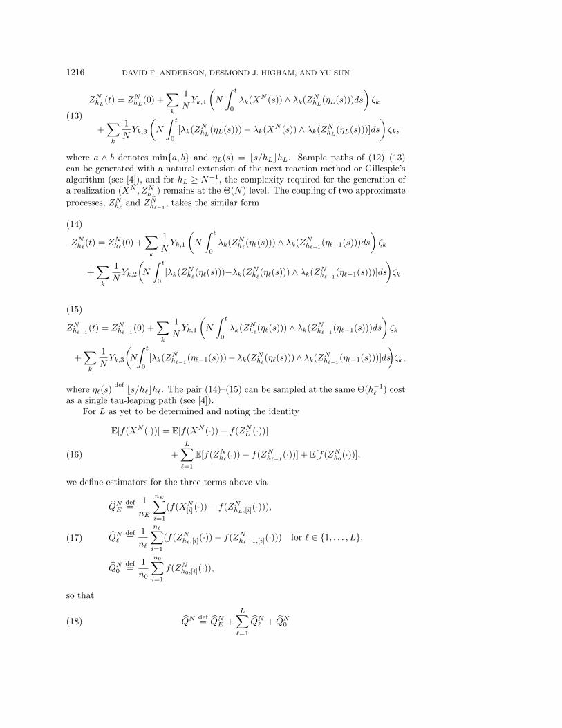
where a ∧ b denotes min{a, b} and ηL(s) = bs/hLchL. Sample paths of (12)–(13)can be generated with a natural extension of the next reaction method or Gillespie’salgorithm (see [4]), and for hL ≥ N−1, the complexity required for the generation ofa realization (XN , ZNhL) remains at the Θ(N) level. The coupling of two approximate

processes, ZNh` and ZNh`−1, takes the similar form

ZNh`(t) = ZNh`(0) +∑k

1

NYk,1

(N

∫ t

0

λk(ZNh`(η`(s))) ∧ λk(ZNh`−1(η`−1(s)))ds

)ζk

+∑k

1

NYk,2

(N

∫ t

0

[λk(ZNh`(η`(s)))−λk(ZNh`(η`(s))) ∧ λk(ZNh`−1(η`−1(s)))]ds

)ζk

(14)

ZNh`−1(t) = ZNh`−1

(0) +∑k

1

NYk,1

(N

∫ t

0

λk(ZNh`(η`(s))) ∧ λk(ZNh`−1(η`−1(s)))ds

)ζk

+∑k

1

NYk,3

(N

∫ t

0

[λk(ZNh`−1(η`−1(s)))−λk(ZNh`(η`(s)))∧λk(ZNh`−1

(η`−1(s)))]ds

)ζk,

(15)

where η`(s)def= bs/h`ch`. The pair (14)–(15) can be sampled at the same Θ(h−1` ) cost

as a single tau-leaping path (see [4]).For L as yet to be determined and noting the identity

E[f(XN (·))] = E[f(XN (·))− f(ZNL (·))]

+

L∑`=1

E[f(ZNh`(·))− f(ZNh`−1(·))] + E[f(ZNh0

(·))],(16)

we define estimators for the three terms above via

QNEdef=

1

nE

nE∑i=1

(f(XN[i](·))− f(ZNhL,[i](·))),

QN`def=

1

n`

n∑i=1

(f(ZNh`,[i](·))− f(ZNh`−1,[i](·))) for ` ∈ {1, . . . , L},

QN0def=

1

n0

n0∑i=1

f(ZNh0,[i](·)),

(17)

so that

QNdef= QNE +

L∑`=1

QN` + QN0(18)


is an unbiased estimator for E[f(XN (·))]. Here, QNE uses the coupling (12)–(13)

between exact paths and tau-leaped paths of step size hL, QN` uses the coupling

(14)–(15) between tau-leaped paths of step sizes h` and h`−1, and QN0 involves singletau-leaped paths of step size h0. Note that the algorithm implicit in (18) produces an

unbiased estimator, whereas the estimator is biased if QNE is left off, as will sometimes

be desirable. Hence, we will refer to estimator QN in (18) as the unbiased estimatorand will refer to

QNBdef=

L∑`=1

QN` + QN0(19)

as the biased estimator. For both the biased and the unbiased estimators, the numberof paths at each level, n0, n`, and nE , will be chosen to ensure an overall estimatorstandard deviation of εN .

We consider the biased and unbiased versions of tau-leaping multilevel MonteCarlo separately.

Biased multilevel Monte Carlo tau-leaping

Here we consider the estimator QNB defined in (19). By Assumption 2.2, we have|E[f(XN (·))]− E[f(ZNhL(·))]| = Θ(hL). Hence, in order to control the bias, we beginby choosing hL = εN and so L = Θ(log(1/εN )) = Θ(logN).

For ` ∈ {1, . . . , L}, let C` be the expected number of random variables required togenerate a single pair of coupled trajectories at level `, and let δN,` be the variance ofthe relevant processes on level `. Let C0 be the expected number of random variablesrequired to generate a single trajectory at the coarsest level. To find n`, ` ∈ {0, . . . , L},we solve the following optimization problem, which ensures that the variance of QNBis no greater than ε2N :

minimizen`

L∑`=0

n`C`(20)

subject to

L∑`=0

δN,`n`

= ε2N .(21)

We use Lagrange multipliers. Since we have C` = K ·h−1` , for some fixed constant K,the optimization problem above is solved at solutions to

∇n0,...,nL,λ

(L∑`=0

n`K · h−1` + λ

(L∑`=0

δN,`n`− ε2N

))= 0.

Taking derivatives with respect to n` and setting each derivative to zero yields

n` =√

λK δN,`h` for ` ∈ {0, 1, 2, . . . , L}(22)

for some λ ≥ 0. Plugging (22) into (21) gives us

L∑`=0

√δN,`h`

=√

λK · ε

2N(23)


and hence, by Assumption 2.3,√λK =

L∑`=0

√δN,`h`≤ CLε−2N N−1/2,(24)

where C is a constant. Noting that L = Θ(log(ε−1N )), we have

λK = Θ

(ε−4N (log εN )

2N−1

).

Plugging this back into (22) and recognizing that at least one path must be generatedto achieve the desired accuracy, we find

n` = Θ(ε−2N N−1h`L+ 1).

Hence, the overall computational complexity is

L∑`=0

n`Kh−1` = Θ

(L∑`=0

ε−2N N−1h`Lh−1` +

L∑`=0

h−1`

)= Θ

(ε−2N N−1(log εN )2 + ε−1N

)= Θ

(N2α−1(logN)2 +Nα

),

recovering row 6 of Table 1.Note that the computational complexity reported for this biased version of mul-

tilevel Monte Carlo tau-leaping is, up to logarithms, the same as that for multilevelMonte Carlo on the diffusion approximation. However, none of the generous assump-tions we made for the diffusion approximation were required.

Unbiased multilevel Monte Carlo tau-leaping

The first observation to make is that the telescoping sum (16) implies that themethod which utilizes E[f(XN (·))− f(ZNhL(·))] at the finest level is unbiased for anychoice of hL. That is, we are no longer constrained to choose L = Θ(| log εN |).

Assume that hL ≥ N−1. Let CE be the expected number of random variables re-quired to generate a single pair of the coupled exact and tau-leaped processes when thetau-leap discretization is hL. To determine n` and nE , we still solve an optimizationproblem,

minimizen`

L∑`=0

n`C` + nLCE(25)

subject toL∑`=0

δN,`n`

+δN,EnE

= ε2N ,(26)

where C` and δN,` are as before and δN,E = Var(f(XN (·))− f(ZNhL(·))).Using Lagrange multipliers again, we obtain

n` =

√λδN,`C`

for ` ∈ {0, 1, 2, . . . , L}(27)

and

nE =

√λδN,ECE

.(28)

Plugging back into (26) and noting that by, Assumption 2.1, C` = Θ(h−1` ) and CE =Θ(N) yields


√λ = ε−2N

(L∑`=0

√δN,`C` +

√δN,ECE

)≤ C(Lε−2N N−1/2 + ε−2N

√hL).(29)

Therefore, plugging (29) back into (27) an (28) and noting n` ≥ 1 and nE ≥ 1, we get

n` =

√λδN,`C`

+ 1 = O

((Lε−2N N−1 + ε−2N

√hLN

)h` + 1

)for ` ∈ {0, 1, 2, . . . , L}

and

nE =

√λδN,`C`

+ 1 = O(Lε−2N N−3/2h1/2L + ε−2N N−1hL + 1).(30)

As a result, the total complexity is

g(hL) = O

(ε−2N N−1L2 + ε−2N

√hLNL+ h−1L + ε−2N

√hLNL+ ε−2N hL +N

)

≤ O

(ε−2N N−1L2 + 2ε−2N

√hLNL+ ε−2N hL + 2N

)= O

(2ε−2N N−1L2 + 2ε−2N hL + 2N

),

where the inequality follows since h−1L ≤ N and we used that 2ab ≤ a2 + b2 in thefinal equality. It is relatively easy to show that the last line above is minimized at

hL =2

(log 2)2NLambertW

(N

2/(log 2)2

)≈ 2

(log 2)2Nlog

(N

2/(log 2)2)

).(31)

Hence, taking hL = Θ(N−1 logN), we have (log hL)2 = Θ((logN)2), and thismethod achieves a total computational complexity of leading order

Θ(ε−2N N−1(logN)2 + ε−2N N−1 logN +N) = Θ(ε−2N N−1(logN)2 +N)

= Θ(N2α−1(logN)2 +N),

as reported in the last row of Table 1.Note here that if we choose hL = 1

N , we get the same order of magnitude for thecomputational complexity. However, the hL in (31) is the optimized solution, meaningthat the leading order constant should be better, and we will see this in Figures 3 and4 in the next section.

5. Computational results. In this section, we provide numerical evidence forthe sharpness of the computational complexity analyses provided in Table 1. We willmeasure complexity by total number of random variables utilized. We emphasize thatthese experiments use extreme parameter choices solely for the purpose of testing thesharpness of the delicate asymptotic bounds.

Example 5.1. We consider the classically scaled stochastic model for the followingreaction network (see [9]):

S1 + S2

k1/N

�k2

S3k3→ S2 + S4.

Letting Xi(t) give the number of molecules of species Si at time t and letting XN (t) =X(t)/N , the stochastic equations are


XN (t) = XN (0) +1

NY1

(Nk1

∫ t

0

XN1 (s)XN

2 (s)ds

)−1−1

10

+1

NY2

(Nk2

∫ t

0

XN3 (s)ds

)11−1

0

+1

NY3

(Nk3

∫ t

0

XN3 (s)ds

)01−1

1

,where we assume XN (0) → (0.2, 0.2, 0.2, 0.2)T as N → ∞. Note that the intensityfunction λ1(x) = κ1x1x2 is globally Lipschitz on the domain of interest, as thatdomain is bounded (mass is conserved in this model).

We implemented different Monte Carlo simulation methods for the estimation ofE[XN

1 (T )] to an accuracy of εN = N−α for both α = 1 and α = 5/4. Specifically,for each of the order one methods we chose a step size of h = εN and required thevariance of the estimator to be ε2N . For midpoint tau-leaping, which has a weak orderof two, we chose h =

√εN . For the unbiased multilevel Monte Carlo method, we

chose the finest time step according to (31). We do not provide estimates for MonteCarlo combined with exact simulation, as those computations were too intensive tocomplete to the target accuracy.

For our numerical example, we chose T = 1 and X(0) = dN · [0.2, 0.2, 0.2, 0.2]T ewith XN (0) = X(0)/N . Finally, we chose k1 = k2 = k3 = 1 as our rate constants. InFigure 1, we provide log-log plots of the computational complexity required to solvethis problem for the different Monte Carlo methods to an accuracy of εN = N−1 foreach of

N ∈ {213, 214, 215, 216, 217}.

In Figure 2, we provide log-log plots for the computational complexity required tosolve this problem for the different methods to an accuracy of εN = N−

54 for each of

N ∈ {29, 210, 211, 212, 213}.

Tables 2 and 3 provide the estimator standard deviations for the different MonteCarlo methods with εN = N−1 and εN = N−

54 , respectively. The top line provides

the target standard deviations.The specifics of the implementations and results for the different Monte Carlo

methods are detailed below.

Diffusion approximation plus Monte Carlo. We took a time step of size h = εNto generate our independent samples. See Figure 1, where the best fit line is y =1.94x − 0.88, and Figure 2, where the best fit line is y = 2.73x − 1.37, which areconsistent with the exponent α in Table 1.

Monte Carlo tau-leaping. We took a time step of size h = εN to generate ourindependent samples. See Figure 1, where the best fit line is y = 1.96x − 1.02, andFigure 2, where the best fit line is y = 2.76x − 1.63, which are consistent with theexponent α in Table 1.


9 9.5 10 10.5 11 11.5 1210

12

14

16

18

20

22

24

Fig. 1. Log-log plots of the computational complexity for the different Monte Carlo methodswith varying N ∈ {213, 214, 215, 216, 217} and εN = N−1.

6 6.5 7 7.5 8 8.5 9 9.510

12

14

16

18

20

22

24

Fig. 2. Log-log plots of the computational complexity for the different Monte Carlo methods

with varying N ∈ {29, 210, 211, 212, 213} and εN = N−54 .

Table 2Actual estimator standard deviations when εN = N−1.

Method Estimator standard deviations

2−13, 2−14, 2−15, 2−16, 2−17

MC and diff. approx 2−13.10, 2−14.02, 2−15.02, 2−16.01, 2−17.00

MC and tau-leaping 2−13.09, 2−14.01, 2−15.01, 2−16.01, 2−17.00

MC and midpoint tau-leaping 2−13.09, 2−14.04, 2−15.03, 2−16.00, 2−17.01

Multilevel diff. approx 2−13.20, 2−14.15, 2−15.11, 2−16.09, 2−17.07

Biased multilevel tau-leaping 2−13.44, 2−14.39, 2−15.39, 2−16.38, 2−17.32

Unbiased multilevel tau-leaping 2−13.29, 2−14.28, 2−15.26, 2−16.21, 2−17.18


Table 3Actual estimator standard deviations when εN = N−5/4.

Method Estimator standard deviations

εN = N−54 2−11.25, 2−12.50, 2−13.75, 2−15.00, 2−16.25

MC and diff. approx 2−11.27, 2−12.51, 2−13.75, 2−15.00, 2−16.25

MC and tau-leaping 2−11.26, 2−12.52, 2−13.76, 2−15.00, 2−16.25

MC and midpoint tau-leaping 2−11.26, 2−12.52, 2−13.76, 2−15.00, 2−16.25

Multilevel diff. approx 2−11.46, 2−12.63, 2−13.85, 2−15.06, 2−16.29

Biased multilevel tau-leaping 2−11.62, 2−12.81, 2−13.99, 2−15.19, 2−16.41

Unbiased multilevel tau-leaping 2−11.34, 2−12.57, 2−13.79, 2−15.03, 2−16.26

Monte Carlo midpoint tau-leaping. We took a time step of size h =√εN . See

Figure 1, where the best fit line is y = 1.44 − 0.86, and Figure 2, where the best fitline is y = 2.10x− 3.53, which are consistent with the exponent α in Table 1.

Our implementation of the multilevel methods proceeded as follows. We choseh` = 2−`, and for εN > 0, we fixed hL = εN and L = dlog(hL)/ log(2)e for the biasedmethods. For each level, we generated N0 independent sample trajectories in orderto estimate δN,`, as defined in section 3. Then we selected

n` =

⌈ε−2N√δN,`h`

L∑j=0

√δN,jhj

⌉+ 1 for ` ∈ {0, 1, 2, . . . , L}

to ensure that the overall variance is below the target ε2N .

Multilevel Monte Carlo diffusion approximation We used N0 = 400 for ourprecalculation of the variances. See Figure 1, where the best fit line is y = 0.99x+2.75,and Figure 2, where the best fit line is y = 1.45x + 2.61, which are consistent withthe exponent α in Table 1.

Multilevel Monte Carlo tau-leaping. We used N0 = 100 for our precalculationof the variances. See Figure 1, where the best fit line is y = 1.12x+ 3.70, and Figure2, where the best fit line is y = 1.56x+ 4.64, which are, up to a log factor, consistentwith the exponent α in Table 1.

Unbiased tau-leaping multilevel Monte Carlo. For our implementation of unbi-ased multilevel tau-leaping, we set hL = 2

N LambertW(N2

)and L = dlog(hL)/ log(2)e.

For each level, we utilized N0 = 100 independent sample trajectories in order to esti-mate δN,`, C`, δN,E , and CE , as defined in section 3. We then selected

n` =

⌈ε−2N

√δN,`C`

(L∑`=0

√δN,`C` +

√δN,ECE

)⌉+ 1 for ` ∈ {0, 1, 2, . . . , L}

and

nE =

⌈ε−2N

√δN,ECE

(L∑`=0

√δN,`C` +

√δN,ECE

)⌉+ 1

to ensure that the overall estimator variance is below our target ε2N . See Figure 1,where the best fit line is y = 1.08x + 3.71, and Figure 2, where the best fit line isy = 1.68x + 2.65, which are, up to a log factor, consistent with the exponent α inTable 1.


9 9.5 10 10.5 11 11.5 1213

13.5

14

14.5

15

15.5

16

16.5

17

Fig. 3. Complexity comparison of unbiased multilevel Monte Carlo tau-leaping when hL = 1N

and hL = 2(log 2)2N

LambertW( N2/(log 2)2

) with εN = N−1.

6 6.5 7 7.5 8 8.5 9 9.513

14

15

16

17

18

19

Fig. 4. Complexity comparison of unbiased multilevel Monte Carlo tau-leaping when hL = 1N

and hL = 2(log 2)2N

LambertW( N2/(log 2)2

) with εN = N−54 .

We also used the unbiased tau-leaping multilevel Monte Carlo method with hL =N−1 to estimate E[X1(1)] to accuracy εN = N−α for both α = 1 and α = 5/4. SeeFigures 3 and 4 for log-log plots of the required complexity when hL = N−1 andhL = 2

(log 2)2N LambertW( N2/(log 2)2 ). As predicted in section 4.2.2, the complexity

required when hL = 2(log 2)2N LambertW( N

2/(log 2)2 ) is lower by some constant factor.

6. Conclusions. Many researchers have observed in practice that approxima-tion methods can lead to computational efficiency relative to exact path simulation.However, meaningful, rigorous justification for whether and under what circumstances


approximation methods offer computational benefit has proved elusive. Focusing onthe classical scaling, we note that a useful analysis must resolve two issues:(1) Computational complexity is most relevant for “large” problems, where many

events take place. However, as the system size grows, the problem convergesto a simpler, deterministic limit that is cheap to solve.

(2) On a fixed problem, in the traditional numerical analysis setting where mesh sizetends to zero, discretization methods become arbitrarily more expensive thanexact simulation because the exact solution is piecewise constant.

In this work, we offer what we believe to be the first rigorous complexity analysisthat allows for systematic comparison of simulation methods. The results, summa-rized in Table 1, apply under the classical scaling for a family of problems parametrizedby the system size, N , with accuracy requirement N−α. In this regime, we can studyperformance on “large” problems when fluctuations are still relevant.

A simple conclusion from our analysis is that standard tau-leaping does offer aconcrete advantage over exact simulation when the accuracy requirement is not toohigh (α < 1); see the first two rows of Table 1. Also, “second-order” midpoint ortrapezoidal tau-leaping improves on exact simulation for α < 2; see row 3 of Table 1.Furthermore, in this framework, we were able to analyze the use of a diffusion, orLangevin, approximation and the multilevel Monte Carlo versions of tau-leaping anddiffusion simulation. Our overall conclusion is that in this scaling regime, using exactsamples alone is never worthwhile. For low accuracy (α < 2/3), second-order tau-leaping with standard Monte Carlo is the most efficient of the methods considered.At higher accuracy requirements (α > 2/3), multilevel Monte Carlo with a diffusionapproximation is best so long as the bias inherent in perturbing the model is prov-ably lower than the desired error tolerance. When no such analytic bounds can beachieved, multilevel versions of tau-leaping are the methods of choice. Moreover, forhigh accuracy (α > 1), the unbiased version is the most efficient, as it does not needto take a time step smaller than εN as the biased version must.

Possibilities for further research along the lines opened up by this work includethe following:

• Analyzing other methods within this framework, for example, (a) multilevelMonte Carlo for the diffusion approximation using discretization methodscustomized for small noise systems or (b) methods that tackle the ChemicalMaster Equation directly using large-scale deterministic ODE technology [24,25].

• Development of tau-leaping methods with weak order greater than two.• Coupling the required accuracy to the system size in other scaling regimes,

for example, to study specific problem classes with multiscale structure [11].• Determining conditions on the system for when the diffusion approximation

and Euler–Maruyama scheme achieve the Θ(h) bias given in Assumption 2.2.• Determining wider classes of models and functionals f for which Assumptions

2.1, 2.2, and 2.3 hold. In particular, most of the results in the literaturerequire λk to be Lipschitz and for f to be a scalar valued function withdomain Zd and bounded second derivatives.

REFERENCES

[1] D. F. Anderson, A modified next reaction method for simulating chemical systems with timedependent propensities and delays, J. Chem. Phys., 127 (2007), p. 214107.

[2] D. F. Anderson, Incorporating postleap checks in tau-leaping, J. Chem. Phys., 128 (2008),p. 054103.


[3] D. F. Anderson, A. Ganguly, and T. G. Kurtz, Error analysis of tau-leap simulationmethods, Ann. Appl. Probab., 21 (2011), pp. 2226–2262.

[4] D. F. Anderson and D. J. Higham, Multilevel Monte-Carlo for continuous time Markovchains, with applications in biochemical kinetics, SIAM Multiscale Model. Simul., 10(2012), pp. 146–179.

[5] D. F. Anderson, D. J. Higham, and Y. Sun, Complexity of multilevel Monte Carlo tau-leaping, SIAM J. Numer. Anal., 52 (2014), pp. 3106–3127.

[6] D. F. Anderson, D. J. Higham, and Y. Sun, Multilevel Monte Carlo for stochastic differentialequations with small noise, SIAM J. Numer. Anal., 54 (2016), pp. 505–529.

[7] D. F. Anderson and M. Koyama, Weak error analysis of numerical methods for stochasticmodels of population processes, SIAM Multiscale Model. Simul., 10 (2012), pp. 1493–1524.

[8] D. F. Anderson and T. G. Kurtz, Continuous time Markov chain models for chemical reac-tion networks, in Design and Analysis of Biomolecular Circuits: Engineering Approachesto Systems and Synthetic Biology, H. Koeppl, D. Densmore, G. Setti, and M. di Bernardo,eds., Springer, Berlin, 2011, pp. 3–42.

[9] D. F. Anderson and T. G. Kurtz, Stochastic analysis of biochemical systems, Stochastics inBiological Systems, 1.2, Springer International Publishing, Cham, 2015.

[10] D. F. Anderson and J. C. Mattingly, A weak trapezoidal method for a class of stochasticdifferential equations, Communi. Math. Sci., 9 (2011), pp. 301–318.

[11] K. Ball, T. G. Kurtz, L. Popovic, and G. Rempala, Asymptotic analysis of multiscaleapproximations to reaction networks, Ann. Appl. Probab., 16 (2006), pp. 1925–1961.

[12] A. F. Bartholomay, Stochastic models for chemical reactions. I. Theory of the unimolecularreaction process, Bull. Math. Biophys., 20 (1958), pp. 175–190.

[13] A. F. Bartholomay, Stochastic models for chemical reactions. II. The unimolecular rate con-stant, Bull. Math. Biophys., 21 (1959), pp. 363–373.

[14] M. Delbruck, Statistical fluctuations in autocatalytic reactions, J. Chem. Phys., 8 (1940),pp. 120–124, https://doi.org/10.1063/1.1750549, http://link.aip.org/link/?JCP/8/120/1.

[15] C. W. Gardiner, Handbook of Stochastic Methods: For Physics, Chemistry and the NaturalSciences, Springer, Berlin, 2002.

[16] M. Gibson and J. Bruck, Efficient exact stochastic simulation of chemical systems with manyspecies and many channels, J. Phys. Chem. A, 105 (2000), pp. 1876–1889.

[17] M. Giles, Multilevel Monte Carlo path simulation, Oper. Res., 56 (2008), pp. 607–617.[18] D. T. Gillespie, A general method for numerically simulating the stochastic time evolution of

coupled chemical reactions, J. Comput. Phys., 22 (1976), pp. 403–434.[19] D. T. Gillespie, Exact stochastic simulation of coupled chemical reactions, J. Phys. Chem.,

81 (1977), pp. 2340–2361.[20] D. T. Gillespie, Approximate accelerated simulation of chemically reacting systems, J. Chem.

Phys., 115 (2001), pp. 1716–1733.[21] P. Glynn and C. han Rhee, Unbiased estimation with square root convergence for SDE

models, Oper. Res., 63 (2015), pp. 1026–1043.[22] M. Hutzenthaler, A. Jentzen, and P. E. Kloeden, Strong and weak divergence in finite

time of Euler’s method for stochastic differential equations with non-globally Lipschitzcontinuous coefficients, Proc. Roy. Soc. A, 467 (2011), pp. 1563–1576.

[23] M. Hutzenthaler, A. Jentzen, and P. E. Kloeden, Divergence of the multilevel MonteCarlo Euler method for nonlinear stochastic differential equations, Ann. Appl. Probab., 23(2013), pp. 1913–1966.

[24] T. Jahnke, On reduced models for the chemical master equation, SIAM Multiscale Model.Simul., 9 (2011), pp. 1646–1676.

[25] V. Kazeev, M. Khammash, M. Nip, and C. Schwab, Direct solution of the chemical masterequation using quantized tensor trains, PLOS Comput. Biol., (2014), http://dx.doi.org/10.1371/journal.pcbi.1003359.

[26] P. E. Kloeden and E. Platen, Numerical Solution of Stochastic Differential Equations, Ap-plications of Mathematics 23, Springer-Verlag, Berlin, 1992.

[27] T. G. Kurtz, The relationship between stochastic and deterministic models for chemical reac-tions, J. Chem. Phys., 57 (1972), pp. 2976–2978.

[28] T. G. Kurtz, Strong approximation theorems for density dependent Markov chains, Stoch.Proc. Appl., 6 (1978), pp. 223–240.

[29] T. G. Kurtz, Representation and Approximation of Counting Processes, Advances in Filteringand Optimal Stochastic Control 42, Springer, Berlin, 1982.

[30] S. C. Leite and R. J. Williams, A constrained Langevin approximation for chemical reactionnetworks, http://www.math.ucsd.edu/∼williams/biochem/biochem.pdf, 2016.

https://doi.org/10.1063/1.1750549

http://link.aip.org/link/?JCP/8/120/1

http://dx.doi.org/10.1371/journal.pcbi.1003359

http://dx.doi.org/10.1371/journal.pcbi.1003359

http://www.math.ucsd.edu/~williams/biochem/biochem.pdf


[31] D. A. McQuarrie, Stochastic approach to chemical kinetics, J. Appl. Probab., 4 (1967),pp. 413–478.

[32] E. Renshaw, Stochastic Population Processes, Oxford University Press, Oxford, 2011.[33] S. M. Ross, Simulation, 4th ed., Academic Press, Burlington, MA, 2006.[34] D. J. Wilkinson, Stochastic Modelling for Systems Biology, 2nd ed., Chapman and Hall/CRC

Press, Boca Raton, FL, 2011.

COMPUTATIONAL COMPLEXITY ANALYSIS FOR MONTE CARLO ...

Documents

Transcript of COMPUTATIONAL COMPLEXITY ANALYSIS FOR MONTE CARLO ...