November 3, 2010 1

COMPUTATIONAL BIOLOGY

Harvey J. GreenbergUniversity of Colorado Denver

Allen G. HolderRose-Hulman Institute of Technology

Computational biology is an interdisciplinary �eld that applies the techniques ofcomputer science, applied mathematics, and statistics to address biological questions.OR is also interdisciplinary and applies the same mathematical and computationalsciences, but to decision-making problems. Both focus on developing mathematicalmodels and designing algorithms to solve them. Models in computational biology varyin their biological domain and can range from the interactions of genes and proteinsto the relationships among organisms and species.

Genes are stretches of deoxyribonucleic acid (DNA), which is sometimes called the�User Manual for Life" and is a double-stranded helix of nucleic acids bonded by base-pairs of complements (a-t, c-g). The central dogma of molecular biology assertsthat information in a cell �ows from DNA to ribonucleic acid (RNA) to protein(note, Francis Crick used `dogma' when he introduced this in 1958 to mean `withoutfoundation' because there was no experimental evidence at that time). Proteins arethe �workers� of the cell, and there is much focus on recognizing, predicting, andcomparing their properties.

Figure 1: Central Dogma of Molecular Biology

Proteins interact either directly by modifying each other's properties through direct

November 3, 2010 2

contact or indirectly by participating in the production and modi�cation of cellularmetabolites. Collectively, the biochemical reactions and the possible intermediatesthat produce a metabolite are called a metabolic pathway, and a metabolic networkis a collection of these pathways. The study of complex networks like that of themetabolism is called systems biology.

Linear Programming: A linear program (LP) is an optimization problem in whichthe variables are in �n, and the constraints and the objective are linear.

Flux Balance Analysis (FBA) � A biochemical process is de�ned by n reactionsthat convert m compounds:

a1jx1 + · · ·+ amjxmkj+⇀↽kj−

b1jx1 + · · ·+ bmjxm,

where xi is the concentration of the i th compound, and kj± is the j th reaction rate (fora 2-way reaction the reverse rate need not equal the forward rate). The correspondingODE is:

dxi(t)

dt=

n∑j=1

(bij − aij)(kj+x

a1j

1 · · ·xamjm − kj−x

a1j

1 · · ·xamjm

)=

n∑j=1

Sijvj(x),

where v is the �ux (production or consumption of mass per unit area per unit time),and Sij is de�ned as a �stoichiometric� (pronounced stoy-kee-uh-me'-trik) coe�cient.These coe�cients are interpreted as:

Sij > 0⇒ rate of compound i produced in reaction j;

Sij < 0⇒ rate of compound i consumed in reaction j.

The following holds asymptotically, provided that the system approaches a steadystate toward equilibrium concentrations x̄:

limt→∞

dx(t)

dt= Sv(x̄) = 0. (1)

Dropping the dependence of the �ux on x̄, the �ux cone is de�ned by this homogeneoussystem plus non-negativity for one-way reactions, indexed by J :

F = {v : Sv = 0, vJ ≥ 0}. (2)

In a metabolic network reactions are distinguished between external and internal.The �ux associated with an external reaction is an exchange between the network ofinterest and the cell's environment.

November 3, 2010 3

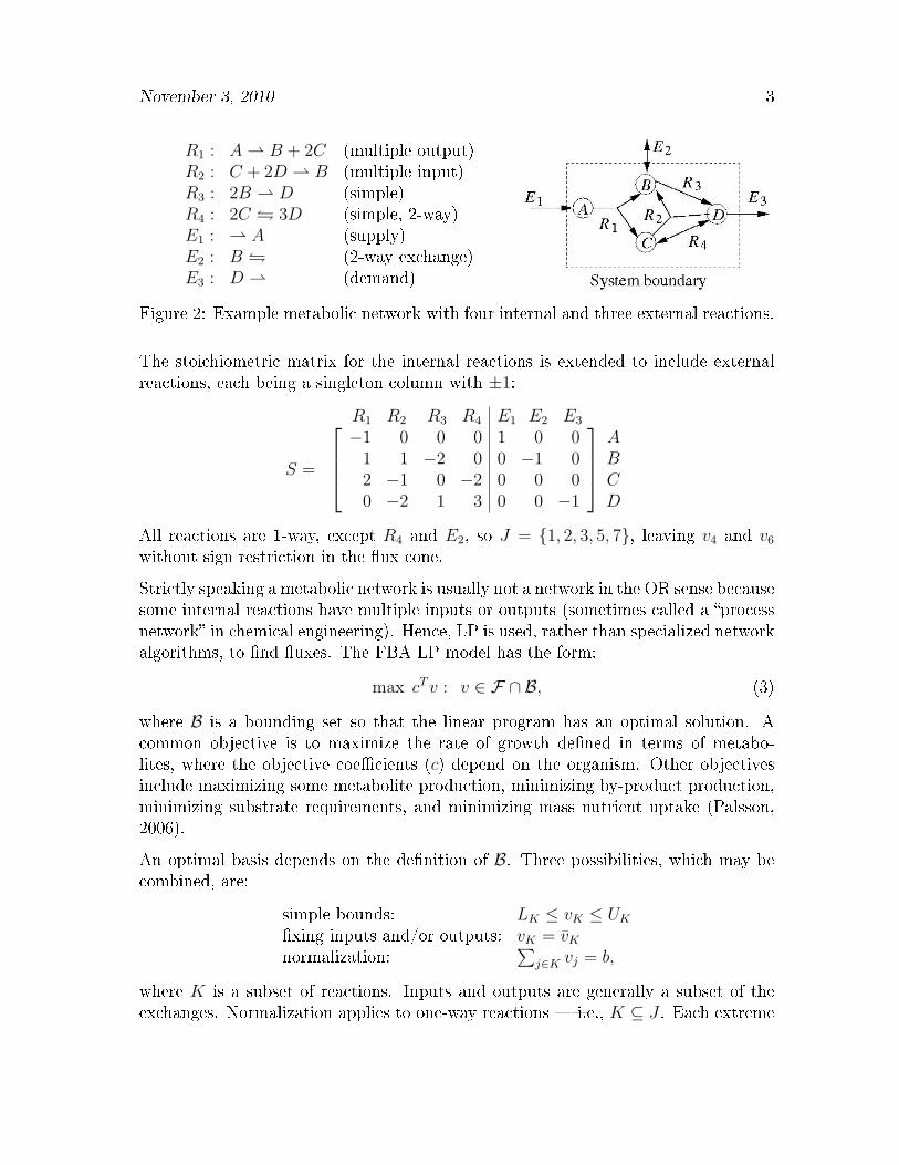
R1 : A ⇀ B + 2C (multiple output)R2 : C + 2D ⇀ B (multiple input)R3 : 2B ⇀ D (simple)R4 : 2C � 3D (simple, 2-way)E1 : ⇀ A (supply)E2 : B � (2-way exchange)E3 : D ⇀ (demand)

Figure 2: Example metabolic network with four internal and three external reactions.

The stoichiometric matrix for the internal reactions is extended to include externalreactions, each being a singleton column with ±1:

R1 R2 R3 R4 E1 E2 E3

S =

−1 0 0 0 1 0 0

1 1 −2 0 0 −1 02 −1 0 −2 0 0 00 −2 1 3 0 0 −1

ABCD

All reactions are 1-way, except R4 and E2, so J = {1, 2, 3, 5, 7}, leaving v4 and v6

without sign restriction in the �ux cone.

Strictly speaking a metabolic network is usually not a network in the OR sense becausesome internal reactions have multiple inputs or outputs (sometimes called a �processnetwork� in chemical engineering). Hence, LP is used, rather than specialized networkalgorithms, to �nd �uxes. The FBA LP model has the form:

max cTv : v ∈ F ∩ B, (3)

where B is a bounding set so that the linear program has an optimal solution. Acommon objective is to maximize the rate of growth de�ned in terms of metabo-lites, where the objective coe�cients (c) depend on the organism. Other objectivesinclude maximizing some metabolite production, minimizing by-product production,minimizing substrate requirements, and minimizing mass nutrient uptake (Palsson,2006).

An optimal basis depends on the de�nition of B. Three possibilities, which may becombined, are:

simple bounds: LK ≤ vK ≤ UK�xing inputs and/or outputs: vK = v̄Knormalization:

∑j∈K vj = b,

where K is a subset of reactions. Inputs and outputs are generally a subset of theexchanges. Normalization applies to one-way reactions � i.e., K ⊆ J . Each extreme

November 3, 2010 4

ray of the �ux cone corresponds to an extreme point of the polytope. The converse isgenerally not true � viz., �xing the �ux of a reaction that transports metabolites inor out of the cell can introduce extreme points with no extreme ray of the �ux conepassing through them.

Pathways are subnetworks with a single biological e�ect. In an ordinary network,where each internal reaction has a single input and output, this is a path. A cut setis de�ned as a set of reactions whose removal renders the stoichiometric equation (1)infeasible for a speci�ed output. For an ordinary network, the OR terminology is adisconnecting set. A minimal cut set for a speci�ed output is, in OR terminology,simply a cut set. For the example, a cut set that separates D from the rest of thenetwork is {R1, R3, R4, E1}. Finding a (minimal) cut set in the general case becomesan IP, using binary variables to block pathways to some speci�ed output.

Nonlinear Programming: A nonlinear program (NLP) is de�ned by having theobjective or some constraint function be nonlinear in the decision variables.

Protein folding � Most proteins go through a process that twists and turnsthe molecules from their primary state of a linear order of amino acids to a nativethree dimensional state in which it remains. That process is called �folding,� and itis theoretically possible to predict a protein's native state, or structure, by knowingits primary state. This determines a protein's function, and some diseases (e.g.,Alzheimer's, Huntington's, and cystic �brosis) are associated with protein misfolding.

Predictive models became possible following the work of Christian B. An�nsen, whoin 1961 published experimental results supporting the Thermodynamic Hypothesis: Aprotein's native state is uniquely determined by its primary sequence; it transitions toa state of minimum free energy. This leads to a nonlinear program with the decisionspace de�ned as the spacial coordinates of atoms, constrained by the biochemistryof a protein's de�ning amino acid sequence. The objective function is a free energydetermined by potential energies from atomic bonds and non-bond interactions.

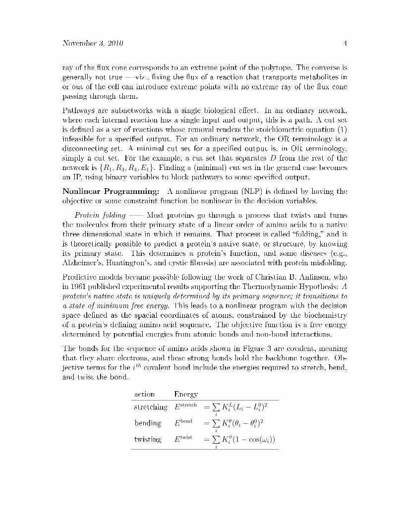
The bonds for the sequence of amino acids shown in Figure 3 are covalent, meaningthat they share electrons, and these strong bonds hold the backbone together. Ob-jective terms for the i th covalent bond include the energies required to stretch, bend,and twist the bond.

action Energy

stretching Estretch =∑i

KLi (Li − L0

i )2

bending Ebend =∑i

Kθi (θi − θ0

i )2

twisting Etwist =∑i

Kφi (1− cos(ωi))

November 3, 2010 5

Figure 3: Covalent bonds along the backbone result in a residue for each of the amino acids.The torsion angles are denoted by Ψ and Φ; ω is the dihedral angle.

The variables are the bond length (L) and the bond angles, θ = (Ψ,Φ) and ω, whichare determined by atomic coordinates. Parameters include target values (L0, θ0).Weight parameters (K) are scale factors that put the energy terms in the same unit;those values can be measured or derived. For example, if it requires 100 kcal/moleto break a bond, and two positive charges within 3.3Å (Angstrom) have at least100 kcal/mole, then total energy is reduced by breaking a bond to keep positivecharges distant. Estimating these values to determine weight parameters is not anexact science, so even these basic energy functions are not exact, and there are otherenergy functions for non-covalent bonds and among non-bonding atoms.

Two common energy functions estimate the electrostatic and Van der Waals interac-tions:

action Energy

Electrostatic Eelec =∑i<j

Kelecij

qiqjdij

Van der Waals Evdw =∑i<j

Kvdwij

((d∗ijdij

)12

− αij(d∗ijdij

)6)

The variables are the pair-wise distances (d), which are determined by the atomiccoordinates. Parameters are the atomic charges (q) and equilibrium distances (d∗).

November 3, 2010 6

Figure 4: The squared deviation ofEstretch and Ebend is convex.

Figure 5: Etwist with ω = 3/2(φ− π).

Figure 6: Eelec depends on the sign ofqiqj. Oppositely-signed atoms attract,so the energy is negative and favorsthem being close.

Figure 7: Lennard-Jones approxima-tion of Evdw for α = 2.

The NLP approach (Floudas and Pardalos, 2000) uses energy principles that underlymolecular dynamics, and these methods attempt to �nd the native state and a path-way to it. In practice, not all parameters are grounded in some physical law. Anenergy function could include contributions from non-bonded and uncharged pairs,based on their distance and radii. Alternatively, known structures can be used topredict an unknown structure, based on their evolutionary similarity. This is called�homology,� and it is focused on determining the native state and not on discerningthe dynamic pathways to reach it.

The multi-modal shape of the energy landscape leads to the Levinthal Paradox: manyproteins reach their native state within milliseconds, yet the number of stable confor-

November 3, 2010 7

mations grows exponentially in the number of amino acids. One explanation is thatproteins fold into a nearby local minimum of the free energy instead of the globalminimum. Global optimization methods based on this principle are called �funnelingmethods.� Another explanation is that the dimension of the problem is not the lengthof the amino-acid sequence but is instead the number of chains that obey patternsnot fully understood. Combinatorial optimization methods based on this principleare called �chain growth� and �zipping and assembly� algorithms.

Comparing Protein Function � A protein's function is determined by its 3Dnative state. The 3D con�rmations of many proteins are known and are available fromthe Protein Database (www.pdb.org). Comparing protein structures relates proteinfunction and collects proteins into functionally similar families that help identify aprotein's functions.

Proteins typically have multiple functional domains, each of which would act as anindependent protein if its amino acid sub-sequence had folded independently. Twoproteins are considered to be functionally similar if they share a (nearly) commondomain. Each domain is composed of secondary structures, notably α-helices andβ-sheets, illustrated in Figure 8. In structure alignment the goal is to best align thesecondary structures between two proteins' domains. The input to the alignmentproblem is a set of coordinates for the Cα atoms for each domain � i.e., the spacialcoordinates for the carbon atoms linked to the side chains (c.f., Figure 3).

November 3, 2010 8

(a) α-helix, most-closely packed arrangement of residues, de�ned by threeparameters: pitch, rise, and turn.

(b) β-sheets form if the backbone is loosely packed, almost fully extended;they can be parallel (left), antiparallel (right), or a mixture.

Figure 8: Secondary structures formed along the backbone de�ne a protein's shape.Dotted lines represent hydrogen bonds; ©R represents a side chain.

To remove a dependency on rigid body motion, structures are often aligned withrespect to pairwise distances, dij, which is a measure between the i th and j th Cαatoms. Let d′ij and d′′kr be the intra-distance measures for the two domains, andconsider the binary variable

xik =

1 if the i th Cα atom of the �rst domain is paired withthe k th Cα atom of the second domain;

0 otherwise.

An optimal pairing between the two domains can be calculated by solving a quadraticinteger program:

max∑i,k,j,r

xikxjrd′ijd′′kr :

∑k

xik ≤ 1,∑i

xik ≤ 1, xik = 0, (i, k) ∈ S,

November 3, 2010 9

where (i, k) ∈ S if the i th and k th Cα atoms are in di�erent types of secondarystructures.

Besides the choice of metric, a variation is to allow pairings between Cα atoms whosesecondary structures are di�erent. This is accommodated by removing the restrictionthat xik = 0 for (i, k) ∈ S and adding penalty terms in the objective: −

∑(i,k)∈S pikxik.

The problem as stated includes the possibility of a non-sequential alignment, i.e.,one in which the Cα atoms can be paired independent of the amino acid sequence.A combinatorial optimization model of alignments that requires the same orderingof the amino acid residues is called �contact map optimization� (Burkowski, 2009;Glodzik and Skolnick, 1994; Goldman et al., 1999).

Integer Programming: An integer program (IP) is an optimization problem inwhich some or all of the variables are restricted to be integer valued. For combinatorialoptimization, the integer values are simply {0, 1}.

Pathway Analysis � Consider the FBA model (3) with added binary variablesassociated with each process with �nite bounds (given or derived), Lj ≤ vj ≤ Uj:

yj =

{1 if vj 6= 0 ;0 otherwise.

Replacing the bound constraints with Ljyj ≤ vj ≤ Ujyj forces vj = 0 if yj = 0. Thiscorresponds to excluding reaction j, which is called a �knock-out.� Drug side-e�ectsare caused by unintended knock-outs, which, if cannot be avoided, can at least beidenti�ed and minimized. In drug design, one may want to block all pathways tosome �nal output. If P is a pathway leading to the targeted output, then adding theconstraint ∑

j∈P

yj ≤ |P | − 1

removes the pathway, where j ∈ P if pathway P contains reaction j.

A cut set can be computed with successive pathway-generation for a speci�ed outputand adding its pathway-elimination constraint. For the example in Figure 2, pathwaysto produce D can be generated by �xing v7 = 1 (and not have y7). The �rst basicoptimal solution uses reactions R1, R3, R4, E1, E3. This leads to the addition of theconstraint:

y1 + y3 + y4 + y5 ≤ 3.

The next pathway generated is R3, E1, and y3 = 0 satis�es both pathway constraints.After eliminating R3, the solution is R1, R4, E1, E3.

Other logical constraints include process con�ict, yj + yj′ ≤ 1 (i.e., inclusion of jrequires exclusion of j′), and process dependence, yj ≥ yj′ (i.e., exclusion of j requiresexclusion of j′), for j 6= j′.

November 3, 2010 10

Rotamer assignment � Part of the protein folding problem is knowing theside-chain conformations � that is, knowing the torsion angles of the bonds (c.f.,Figure 3). The rotation about a bond is called a �rotamer,� and there are librariesthat give con�guration likelihoods, for each amino acid (from which energy valuescan be derived). The Rotamer Assignment (RoA) Problem is to �nd an assignmentof rotamers to sites that minimizes the total energy of the molecule. For the proteinfolding problem, the amino acid at each site is known. There are about 10 to 50rotamers per amino acid, depending on what else is known (such as knowing that theamino acid is located in a helix), so there are about 10n to 50n rotamer assignmentsfor a protein of length n.

Let r be in the set of rotamers that can be assigned to site i, denoted by Ri, and let

xir =

{1 if rotamer r is assigned to site i ;0 otherwise.

Then, the Quadratic Binary Program (QBP) for the RoA problem is the quadraticsemi-assignment problem:

min∑i

∑r∈Ri

(Eirxir +

∑j>i

∑t∈Rj

Eirjtxirxjt

):∑

r∈Rixir = 1 ∀ i, x ∈ {0, 1}.

The objective function includes two types of energy: (1) within a site, Eir, and (2)between rotamers of two di�erent sites, Eirjt for i 6= j. The summation conditionj > i avoids double counting, where Eirjt = Ejtir.

Besides its role in determining a protein's structure, the RoA Problem is useful indrug design. Speci�cally, the RoA Problem can be used to determine a minimum-energy docking site for a ligand, which is a small molecule such as a hormone orneurotransmitter that binds to a protein and modi�es its function. The ligand-proteindocking problem is characterized by only a few sites, and if the protein is known, thedimensions are small enough that the RoA Problem can be solved exactly. However,if the protein is to be engineered, then there can be about 500 rotamers per site (20acids @ 25 rotamers each), in which case solutions are computed with metaheuristicsor approximation algorithms. There are other bioengineering problems associatedwith the RoA Problem, such as determining protein-protein interactions. While themathematical structure is the same, the applications have di�erent energy data, whichcan a�ect algorithm performance (Forrester and Greenberg, 2008).

See (Clote and Backofen, 2000; Jones and Pevzner, 2004; Lancia, 2006) for more.

Dynamic Programming: This is a computational approach to sequential decision-making. Two fundamental biological sequences are taken from the alphabet of nucleic

November 3, 2010 11

acids, {a,c,g,t}, and from the alphabet of amino acids, {A,R,N,D,C,Q,E,G,H,I,L,K,M,F,P,S,T,W,Y,V}. The former is a segment of DNA (or RNA if u replaces t �i.e., uracil instead of thymine); the latter is a protein segment.

Sequence Alignment � Two sequences can be optimally aligned by dynamicprogramming, where �optimal� is one that maximizes an objective that has two parts:

1. a scoring function, given in the form of an m×m matrix S, where m is the sizeof the alphabet. The value of Sij measures a propensity for the i th alphabet-character in one sequence to align with the j th alphabet-character in someposition of the other sequence.

Example: Let s = agt and t = gtac. If the �rst character of s is aligned withthe �rst character of t, then the score is Sag, which is the propensity for ato be aligned with g.

2. a gap penalty function, expressed in two parts: a ��xed cost� of beginning a gap,denoted Gopen, and a cost to �extend� the gap, denoted Gext.

Example: Let s = agt and t = gtac. One alignment is agt-gtac

, which puts a

gap at the end of the �rst sequence.

A gap is called an �indel� because it can be either an insertion into one sequence ora deletion from the other sequence: insert - delete

↓ a ↑ If one sequence evolved directly

from the other, the evolutionary operation is determined by their time-order. If theyhave a common ancestor, they evolved along di�erent paths, resulting in the indelwhen comparing them. The evolutionary biology explains why sequences can be moresimilar than a simple alignment (without gaps) may suggest.

Figure 9 shows three di�erent alignments for the two nucleic acid sequences, agtand gtac. Scores are shown for the following scoring matrix and do not account forgapping:

a c g t

S =

6 1 2 11 6 1 22 1 6 11 2 1 6

.a

c

g

t

November 3, 2010 12

agt-- -a-gt agt-

|| | | |||

-gtac gtac- gtac

Score = 12 Score = 2 Score = 4

Figure 9: Three alignments for two sequences.

If the objective is a linear a�ne function of gap lengths, the total objective functionfor the 2-sequence alignment problem is:∑

i,j

Ssitj −Gopen(Ns +Nt)−Gext(Ms +Mt),

where the sum is over aligned characters, si from sequence s with tj from sequencet. The number of gaps opened is Ns in sequence s and Nt in sequence t; the numberof gap characters (-) is Ms in sequence s and Mt in sequence t. In the example ofFigure 9, if Gopen=2 and Gext=1, the gap penalties are 7, 9, and 3, respectively.

The alphabet is extended to include the gap character, with S extended to includegap extension, as Sa- = S-a = Gext for all a in the alphabet. (So, Gext includes thepenalty for the �rst alignment with -.) Let si denote the subsequence (s1, . . . , si),with s0 = ∅. Here is the DP recursion for Gopen=0:

F (si, tj) = max

F (si−1, tj−1) + Ssitj matchF (si−1, tj) + Ssi- insert - into tF (si, tj−1) + S-tj insert - into s.

(4)

The initial conditions are:

F (∅, ∅) = 0

F (si, ∅) = F (si−1, ∅) + Ssi-, i = 1, . . . , |s|F (∅, tj) = F (∅, tj−1) + S-tj , j = 1, . . . , |t|.

The DP recursion (4) is for �global alignment,� and it has been extended to allowGopen > 0 and to not penalize leading or trailing gaps (allowing a short sequence to bealigned with a large one meaningfully). Local alignment is �nding maximal substrings(contiguous subsequences) with an optimal global alignment having maximum score(Gus�eld, 1997; Waterman, 1995).

Sequences from many species can be compared simultaneously in a Multiple SequenceAlignment (MSA). One way to evaluate an MSA is by summing pairwise scores.Figure 10 shows an example. The sum-of-pairs score, based on the scoring matrix S,is shown for each column. For example, column 1 has 3Saa + 3Sac = 3. The sum of

November 3, 2010 13

pairwise scores for column 2 is zero because gap scores are not shown by columns;they are penalized for each sequence (rows of alignment) with Gopen=2 and Gext=1.The total objective value is 152− 37 = 115.

Gap penaltya - g a g t - a c t - - - 11a a g t a t - - a t - - - 9a - - t a t a a - - - - t 10c - g t a - - a c t c c t 7

score: 21 0 18 21 24 18 0 18 8 18 0 0 6 37Total = 152

Figure 10: A multiple alignment of four sequences.

MSA is a computational challenge to exact DP due to the combinatorial explosion ofthe state space, but one could use approximate DP or formulate MSA as an IP.

Phylogenetic Tree Construction � Phylogeny is the evolutionary history of somebiological entity. A phylogenetic tree (PT) is a graphical presentation of a phylogeny.A leaf represents an Operational Taxonomic Unit (OTU), which can be various levels� e.g., species, genes, pathways, enzymes, microbial communities, bacterial strains.Each edge, or branch, is a relation between pairs of OTUs. Each internal node isconstructed so that the resulting PT is consistent with the OTU data, and the rootrepresents a common ancestor of the OTUs.

Example. Consider �ve OTUs and an MSA of DNA sites with six base-pairs:

siteOTU 1 2 3 4 5 6A c a g a c a

B c a g g t a

C c g g g t a

D t g c g t a

E t g c a c t

November 3, 2010 14

Figure 11: The example maximum-parsimony PT has eight mutations, shown on thebranches. (All other PTs have more than 8.)

If the number of mutations is the distance between two sequences, then the distancebetween OTUs is the length of the unique path between them in the PT. The examplehas the distance matrix:

D =

A B C D E02 03 1 05 3 2 08 6 5 3 0

ABCDE

This is not the same as the MSA distance. For example, D(A,E) = 8 in the PT butis only 4 in the MSA.

Regardless of how the distance matrix is derived (MSA or not), there may not exist aPT that satis�es speci�ed distances. For that to be true it is necessary and su�cientthat the metric be �additive� � i.e., for any four leaves, there exist labels i, j, k, `such that

D(i, j) +D(k, `) = D(i, `) +D(j, k) ≥ D(i, k) +D(j, `).

The reason for this is that there must be some splitting i, k from j, ` with an internalbranch:

Additivity does not usually hold, so the problem is to construct a PT whose associatedleaf-distance matrix, D, minimizes some function of nearness to the given D0, such as

November 3, 2010 15

||D −D0||. This problem is NP-hard. Heuristics include sequential clustering: Un-weighted/Weighted Pair Group Method with Arithmetic Mean (UPGMA/WPGMA)and neighbor-joining algorithms.

There may be multiple PTs, which generally come from di�erent data � e.g., onefrom an MSA of a DNA segment, another from the maximum likelihood of someproperty. If a series of edge-contractions is applied to a PT, the resulting PT iscalled a �re�nement� and the original is called a �re�ner.� Two trees are compatibleif they have a common re�ner. One problem is to determine whether two PTs arecompatible, and if so, what is their common re�ner? If incompatible, how is a PTconstructed that has some agreement with the given PTs?

Figure 12: PTs T1, T2 are compatible.

A Matrix Representation with Parsimony (MRP) of a PT with k internal nodes is abinary matrix de�ned as:

Mij =

{1 if internal node j is in the (unique) path from the root to OTU i ;0 otherwise.

Conversely, given a binary matrix, if it has an associated PT, it is called a �perfectphylogeny.�

Given two PTs for the same OTUs with MRPs, M1,M2, their column-union is[M1 M2].

Theorem. Two PTs are compatible if, and only if, their MRP column-union repre-sents a perfect phylogeny.

The trees in Figure 12 have the MRP column-union:

M =

M1 M21 01 00 10 1

ABCD

November 3, 2010 16

This is the MRP of the common re�ner in Figure 12 and represents a perfect phy-logeny.

Figure 13: PTs T1, T2 are incompatible.

The MRP column-union of the PTs in Figure 13 is:

M =

M1 M20 0 0 01 0 1 11 1 1 01 1 1 1

ABCD

M does not correspond to any PT. (After drawing A,C,D with four internal nodesas the path to D, OTU B cannot be drawn with the path 0-1-3-4 without introducingthe cycle, 1-2-3-1.)

Suppose the trees are incompatible. A Maximum Agreement Subtree (MAST) is are�ned subtree with the greatest number of leaves.

Figure 14: A Maximum Agreement Subtree with 2 of the 4 OTUs.

The DP recursion for two subtrees (Steel and Warnow, 1993) is nontrivial. The stateis a pair of subtrees with speci�ed roots, (T r1 , T

s2 ). Each tree has an inclusion-ordered

sequence of such subtrees, which is computed during the recursion. The decision spaceto compute MAST (T r1 , T

s2 ), given MAST (T r

′1 , T

s′2 ) for (T r

′1 , T

s′2 ) ≺ (T r1 , T

s2 ), requires

the computation of a maximum weighted-matching on the complete r-s bipartitegraph, weighted with {MAST (r′, s′)}.

Whereas MAST uses an intersection of PT information, a supertree uses their union.Construction methods vary, and some of the criteria address common order preser-vation. An agreement supertree, T , is a minimal tree such that each Ti is a re�nedsubtree of T .

November 3, 2010 17

Figure 15: An Agreement Supertree of the trees in Figure 14.

Markov Chains and Processes: A stochastic process has the Markov property ifthe transition from one state to the next depends on only the current state. Classicalmodels include the evolution of some biological state over time (Allen, 2003). Molec-ular applications of Markov models also consider ordered sequences of nucleotides(viz., DNA and RNA) and amino acids (viz., proteins).

CpG island recognition � In the human genome the appearance of the dinu-cleotide CG is rare because it causes the cytosine (C) to be chemically modi�ed bymethylation, which causes it to mutate into thymine (T). Methylation is suppressedaround the promoters, or start regions, of many genes, and there are more CG dinu-cleotides than elsewhere. Such regions are called �CpG islands,� and they are typicallya few hundred bases long. (CpG is used instead of CG to avoid confusion with a C-G

base pair; the p is silent.) The recognition problem is: Given a short segment of agenomic sequence, decide if it is part of a CpG island.

Two Markov chains are de�ned: P+ is the state-transition matrix within a CpG island;P− is the state-transition matrix outside a CpG island. Each is applied to the givensequence and the log-odds ratio determines which is more likely.

Example. Consider a �rst-order Markov chain model with transition matrices de-termined by the frequencies in a database having more than 60,000 human DNAsequences:

A C G T A C G T

P+ =

0.18 0.27 0.43 0.120.17 0.37 0.27 0.190.16 0.34 0.38 0.120.08 0.36 0.38 0.18

P− =

0.30 0.20 0.29 0.210.32 0.30 0.08 0.300.25 0.25 0.30 0.200.18 0.24 0.29 0.29

Given the sequence AACTTCG, its total log-odds ratio is

6∑i=1

log2

(P+sisi+1

/P−sisi+1

)= −0.737 + 0.433− 0.659− 0.688 + 0.585 + 1.755 = 0.6888.

The conclusion is that the DNA segment is in a CpG island.

November 3, 2010 18

There is enough data to support the use of the more-accurate 5th-order Markov chain,whose 6-tuples correspond to two coding regions. At least 45 6-tuples are requiredin the database to estimate the conditional probabilities, Pr(x6 |x1x2x3x4x5), whichdirectly yield the state-transition probabilities:

Pr(y1y2y3y4y5 |x1x2x3x4x5) =

{Pr(x6 |x1x2x3x4x5) if y = (x2x3x4x5x6);0 otherwise.

For the particular example, there are only two state transitions, and the same databasegives the transition probabilities:

P+(C | AACTT) = 0.4 P−(C | AACTT) = 0.2

P+(G | ACTTC) = 0.1 P−(G | ACTTC) = 0.3

In this case the more accurate 5th-order chain yields the log-odds ratio log2 0.4/0.2 +log2 0.1/0.3 = −0.585, and the conclusion is that the DNA segment is not in a CpG

island.

A host of related problems use the same Markov model. For example, transcriptionsplices the DNA into coding regions, called �exons,� removing the remainder, called�introns� (misnamed �junk DNA�). A structure recognition problem is to identifyexons vs. introns.

Many of the structure recognition, comparison, and prediction problems have hid-den states, but emissions are observed according to a known probability. These are�Hidden Markov Models� (HMMs) and are central in modern biology (Durbin et al.,1998).

Queueing Theory: A queue in a system is any set of objects awaiting service, andservice is some process(es) involving the object.

T-cell signaling � A T-cell is a type of white blood cell distinguished by hav-ing a receptor � an ability to bind to other molecules. The receptor interacts withintracellular pathway components, starting a cascade of protein interactions called�signal transduction.� A way to view this process is that a T-cell receptor (TCR)enters a queue upon activation and goes through a series of processes, such as phos-phorylation (Wedagedera and Burroughs, 2006). Service completion is de�ned by thedeactivation of the TCR, returning it to the inactive pool; however, it is possible thatthe T-cell's service is aborted before it completes service. Of interest is the probabil-ity of activation � i.e., in service for some threshold of time. If it completes serviceand detects infection, the T-cell signals cell death (called �apoptosis,� pronounced�ap'o-to's��s; the `p' is silent).

Other queueing models apply to genetic networks, allowing signals that a�ect thepopulation to enter and leave the system (Arazi et al., 2004; Jamalyaria et al., 2005).

November 3, 2010 19

This applies queueing to a broad range of self-assembly systems � i.e., form anarrangement without external guidance.

Simulation: Dynamical state evolution is fundamental in both classical mathe-matical biology and modern systems biology. Evolution and biochemical pathwaysare prime examples; the underlying state-transition structure and the sheer size aresu�cient to need simulation.

The kinetic laws of a biosystem depend upon the objects, particularly their scale (viz.,molecules vs. cells). The deterministic rate equations have the form:

dxidt

= fi(x; k) for i = 1, . . . ,m,

where x is the system state (e.g., concentrations of m metabolites) and k is a vectorof parameters, called rate constants.

Sources of randomness can be intrinsic � e.g., errors in parameter estimation, orextrinsic � e.g., protein production in random pulses (Meng et al., 2004). To dealwith reaction uncertainty, Gillespie (2008, 1977) introduced the probability equation:

Pr(x; t+ dt) =∑

r ar(x− vr) dt+ Pr(x; t) (1−∑

r ar(x) dt) ,

where ar(x) dt is the probability that reaction r occurs in the time interval (t, t+ dt),changing the state from x to x + vr. The �rst summation represents being onereaction removed from the state x; the last term represents having no reaction duringthe interval.

Auto-regulatory network � Puchalka and Kierzek (2004) consider a metabolicnetwork with regulatory processes and random �uctuations in gene expression. UsingGillespie's equation, given the state x at time t, the probability that the next reaction,r, occurs during (t+ τ, t+ τ + dt) is given by:

Pr(τ, r |x, t) = ar(x) e−P

j aj(x)τ .

The simulation is run by generating (τ, r) using this joint density function. Thesimulation also allows for pulse production � a receptor site may be on or o� toregulate gene expression (restricting the choice of r).

Other models use rare-event simulation, such as for tumor development (Abbott,2002). Simulation is used in systems biology to understand how non-dominant path-ways a�ect assembly kinetics (Zhang and Schwartz, 2006).

Game Theory: The central idea of game theory is that each player has its ownobjective to optimize. Historically, evolutionary biologists used game theory to modelnatural selection (Maynard Smith, 1982; Perc and Szolnoki, 2010). In OR, game the-ory is used to model competition for economic resources, and this extends to modeling

November 3, 2010 20

species-invasion into an existing ecosystem. The same game model applies to propa-gation of tumor cells that can mutate in minutes to create a cancer population thatoverwhelms normal cells (Tomlinson, 1997). New applications are at the molecularscale, such as the following example.

Protein binding � There are two sets of players: protein classes (includingdrugs) and DNA binding sites. Their joint strategies result in allocation of proteinsto sites. Sites seek to maximize their occupancy; proteins seek to minimize excessbinding. Sites compete for nearby proteins; proteins choose target sites to whichthey transport. (Mechanisms to achieve these choices are not well understood.) Thea�nity for protein i to bind to site j is denoted by the constant Kij, but this appliesonly if the protein is in the proximity of the site.

Let i = 1, . . . , Np index proteins and j = 1, . . . , Ns index sites, and consider theparameters:

νi = nuclear concentration,Eij = transport a�nity,Kij = binding a�nity.

A protein's decision variable is its fractional transported amounts, pi = (pi0, . . . , piNs

),where pi0 = 1 −

∑Ns

j=1 pij is the portion of protein i not allocated to a site. A site's

decision variable is its choice of binding frequency, sj = (sj0, . . . , sjNp

), where sj0 =

1 −∑Np

i=1 sij is the portion of time that site j is unoccupied. There are resource

constraints on joint strategies, notably sji ≤ pijνi for i > 0 � i.e., binding cannotexceed allocated concentration.

A solution is a joint strategy (p, s) that satis�es the optimality criteria:

pi ∈ argmaxpi∈P (s)

{f ip(pi, s)} sj ∈ argminsj∈S(p)

{f js (p, sj)},

where fp, fs denote objective functions for each protein and site, and P ⊆ �Ns+1+ , S ⊆

�Np+1+ denote feasible regions, each dependent on the other decisions. An example of

objective functions are maximizing total binding a�nity and minimizing the amountof protein not assigned:

f ip(pi, s) =

Ns∑j=1

Eijpij(1− s

j0)

f js (sj, p) = sj0

Np∑i=1

Kij(pijνi − s

ji ).

With mild modi�cations, a solution exists and there is a simple algorithm to �nd it(Pérez-Breva et al., 2006).

November 3, 2010 21

This game model is a simpli�cation of a broader biology, where sites can coordinate,not just compete, and proteins can form complexes to bind to the same site. Thereare also promoters that bind to a protein in order to send it to another site. Althoughcurrent thinking is that proteins roam randomly until they bump into an unoccupiedsite for which they have a�nity, the game model attributes a purposeful behavior toproteins, suggesting that they choose to transport to some site. While this rationalbehavior is not due to intelligence, it could be due to an environmental context thatis not yet understood and whose net e�ect makes proteins behave as if they arerational players.

References

R. Abbott. CancerSim: A computer-based simulation of Hanahan andWeinberg's Hallmarksof Cancer. Masters thesis, The University of New Mexico, Albuquerque, NM, 2002.

L. J. S. Allen. An Introduction to Stochastic Processes with Applications to Biology. PearsonEducation, Upper Saddle River, NJ, 2003.

A. Arazi, E. Ben-Jacob, and U. Yechiali. Bridging genetic networks and queueing theory.Physica A: Statistical Mechanics and its Applications, 332:585�616, 2004.

F. Burkowski. Structural Bioinformatics: An Algorithmic Approach. Mathematical andComputational Biology. Chapman & Hall/CRC, Boca Raton, FL, 2009.

P. Clote and R. Backofen. Computational Molecular Biology. John Wiley & Sons, New York,NY, 2000.

R. Durbin, S. Eddy, A. Krogh, and G. Mitchison. Biological Sequence Analysis: ProbabilisticModels of Proteins and Nucleic Acids. Cambridge University Press, Cambridge, UK, 1998.

C. A. Floudas and P. M. Pardalos, editors. Optimization in Computational Chemistry and

Molecular Biology: Local and Global Approaches. Kluwer Academic Publishers, 2000.

R. J. Forrester and H. J. Greenberg. Quadratic binary programming models in computationalbiology. Algorithmic Operations Research, 3(2):110�129, 2008.

D. T. Gillespie. Simulation methods in systems biology. In M. Bernardo, P. Degano, andC. Zavattaro, editors, Formal Methods for Computational Systems Biology, LNCS 5016,pages 125�167. Springer, 2008.

D. T. Gillespie. Exact stochastic simulation of coupled chemical reactions. The Journal of

Physical Chemistry, 81(25):2340�2361, 1977.

A. Glodzik and J. Skolnick. Flexible algorithm for direct multiple alignment of proteinstructures and sequences. Bioinformatics, 10(6):587�596, 1994.

November 3, 2010 22

D. Goldman, S. Istrail, and C.H. Papadimitriou. Algorithmic aspects of protein structuresimilarity. In 40th Annual Symposium on Foundations Of Computer Science (FOCS),pages 512�521. IEEE Computer Society Press, 1999.

D. Gus�eld. Algorithms on Strings, Trees, and Sequences: Computer Science and Compu-

tational Biology. Cambridge University Press, Cambridge, UK, 1997.

F. Jamalyaria, R. Rohlfs, and R. Schwartz. Queue-based method for e�cient simulationof biological self-assembly systems. Journal of Computational Physics, 204(1):100�120,2005.

N. C. Jones and P. A. Pevzner. An Introduction to Bioinformatics Algorithms. MIT Press,Cambridge, MA, 2004.

G. Lancia. Applications to computational molecular biology. In G. Appa, P. Williams,P. Leonidas, and H. Paul, editors, Handbook on Modeling for Discrete Optimization, vol-ume 88 of International Series in Operations Research and Management Science, pages270�304. Springer, 2006.

J. Maynard Smith. The Theory of Games and the Evolution of Animal Con�icts. CambridgeUniversity Press, Cambridge, UK, 1982.

T. C. Meng, S. Somani, and P. Dhar. Modeling and simulation of biological systems withstochasticity. In Silico Biology, 4(0024), 2004.

B. Ø. Palsson. Systems Biology: Properties of Reconstructed Networks. Cambridge Univer-sity Press, New York, NY, 2006.

M. Perc and A. Szolnoki. Coevolutionary games � A mini review. BioSystems, 99(2):109�125, 2010.

L. Pérez-Breva, L. E. Ortiz, C-H. Yeang, and T. Jaakkola. Game theoretic algorithms forprotein-DNA binding. In Proceedings of the 12th Annual Conference on Neural Informa-

tion Processing (NIPS), Vancouver, Canada, 2006.

J. Puchalka and A. M. Kierzek. Bridging the gap between stochastic and deterministicregimes in the kinetic simulations of the biochemical reaction networks. Biophysical Jour-nal, 86(3):1357�1372, 2004.

M. Steel and T. Warnow. Kaikoura tree theorems: Computing the maximum agreementsubtree. Information Processing Letters, 48(3):77�82, 1993.

I. P. M. Tomlinson. Game-theory models of interactions between tumour cells. European

Journal of Cancer, 33(9):1495�1500, 1997.

M.S. Waterman. Introduction to Computational Biology: Maps, Sequences, and Genomes

(Interdisciplinary Statistics). Chapman & Hall/CRC, Boca Raton, FL, 1995.

November 3, 2010 23

J. R. Wedagedera and N. J. Burroughs. T-cell activation: A queuing theory analysis at lowagonist density. Biophysical Journal, 91:1604�1618, 2006.

T. Zhang and R. Schwartz. Simulation study of the contribution of oligomer/oligomerbinding to capsid assembly kinetics. Biophysical Journal, 90:57�64, 2006.