Computational Biology - Computer Science Departmentfeng/teaching/compbio_2015_I.pdf ·...
104
Computational Biology Jianfeng Feng Warwick University (many slides are from Dr. M. Lindquist) http://www.dcs.warwick.ac.uk/~feng/Comp_Biol.html
Transcript of Computational Biology - Computer Science Departmentfeng/teaching/compbio_2015_I.pdf ·...

Computational Biology
Jianfeng Feng
Warwick University
(many slides are from Dr. M. Lindquist)
http://www.dcs.warwick.ac.uk/~feng/Comp_Biol.html

Brain Science with Big Data:
Data Acquisition, machine learning and networks
International brain projects: EU HBP, 1 B Euros
USA BRAIN, 4.5 B Dollars

Module Purposes
• Learn how to deal with big data in a concrete
example: a nice piece of work to demonstrate
the power and trouble of big data
• Understand how to tackle the most complex
organ in the universe
• Transfer skills: apply the same techniques to
other areas with big data

Outline (week 1 and 2)
1. Introduction
2. Basic MRI
3. Image Formation
4. K-space

Outline (week 1 and 2)
1. Introduction
2. Basic MRI
3. Image Formation
4. K-space
5. fMRI signal and noise
6. fMRI data structure
7. Pre-processing

Outline (week 1 and 2)
1. Introduction
2. Basic MRI
3. Image Formation
4. K-space
5. fMRI signal and noise
6. fMRI data structure
7. Pre-processing Able to use SPM to extract signals

first
secondthird
fouth?
Brain research
1831
1785
1970s
2020?AI
Are we facing another revolution?
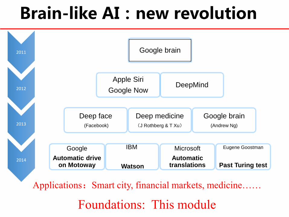
Google brain
Apple Siri
Google NowDeepMind
Deep face
(Facebook)
Deep medicine
(J Rothberg & T Xu)
Google brain
(Andrew Ng)
Automatic drive on Motoway
IBM
Watson
Microsoft
Automatic translations
Eugene Goostman
Past Turing test
Applications:Smart city, financial markets, medicine……
Foundations: This module
Brain-like AI:new revolution
2011
2012
2013
2014

Introduction to fMRI
behaviourbrainregionsmicorcircuitsNeuronssynapsesProtein
Genetics
Environments

Introduction to fMRI
behaviourbrainregionsmicorcircuitsNeuronssynapsesProtein
Genetics
Environments

Neuron
Neuron
The Architecture of the Neuron

Neuronal Activities
Vertical white bar: spike
soma
Dendrite
axon
synapse

Brain works in this way: Spiking neuronal network
Black dot: neuron
White dot: spike
The average of spikes is
called local field potential which is the signal we can measure
= average activity
of one time window
Rossoni E. et al. (2008), Plos Comp Biol.
Local field potential =

Can we understand our brain?
Can we observe neuronal activity?
Multi-billion Dollars Question

Can we understand our brain?
Can we observe neuronal activity?
Multi-billion Dollars Question

Brain Imaging
• In recent years there has been explosive interest
in using imaging techniques to explore the inner
workings of the human brain.
• Brain imaging data has found applications in a
wide variety of fields, such as psychology,
neuroscience, economics, political science,
and medicine.

• Brain imaging can be separated into two
major categories:
– Structural brain imaging
– Functional brain imaging
• There exist a number of different modalities
for each category.
Brain Imaging

Structural Brain Imaging
• Structural brain imaging deals with the study
of brain structure and the diagnosis of
disease and injury.
• Modalities include:
– computed axial tomography (CAT),
– magnetic resonance imaging (MRI),
– positron emission tomography (PET), and
– Diffusion tensor image (DTI)

Structural Brain Imaging
• Structural brain imaging deals with the study
of brain structure and the diagnosis of
disease and injury.
• Modalities include:
– computed axial tomography (CAT),
– magnetic resonance imaging (MRI),
– positron emission tomography (PET), and
– Diffusion tensor image (DTI)

MRI: your brain structure
Proton Density T1 T2
Principle: Different materials have different magnetic fields
real One modality another one

MRI: your brain structure
Proton Density T1 T2
Principle: Different materials have different magnetic fields
real One modality another one

Functional Brain Imaging
• Functional brain imaging can be used to
study both cognitive and affective processes.
• Modalities include:
– functional magnetic resonance imaging (fMRI),
– electroencephalography (EEG), and
– magnetoencephalography (MEG).

Functional Brain Imaging
• Functional brain imaging can be used to
study both cognitive and affective processes.
• Modalities include:
– functional magnetic resonance imaging (fMRI),
– electroencephalography (EEG), and
– magnetoencephalography (MEG).
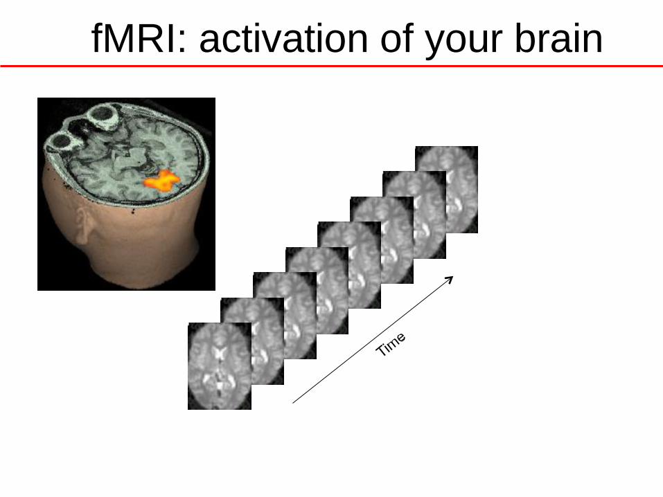
fMRI: activation of your brain
Properties
• Each functional imaging modality provides a
different type of measurement of the brain.
• They also have their own pros and cons with regards
to spatial resolution, temporal resolution and
invasiveness.
• Functional MRI provides a nice balance between these
properties and has become the dominant functional
imaging modality in the past decade.

Functional MRI
• Functional magnetic resonance imaging (fMRI) is a
non-invasive technique for studying brain activity.
• During the course of an fMRI experiment, a
series of brain images are acquired while the
subject performs a set of tasks or at resting.
• Changes in the measured signal between
individual images are used to make inferences
regarding (task-related) activations or construct
networks in the brain.

fMRI Data
• Each image consists of ~100,000 'voxels' (cubic
volumes that span the 3D space of the brain).

• Each image consists of ~100,000 'voxels' (cubic
volumes that span the 3D space of the brain).
fMRI Data

• Each image consists of ~100,000 'voxels' (cubic
volumes that span the 3D space of the brain).
• Each voxel corresponds to a spatial location and
has a number associated with it that represents
its intensity (density or activity).
39
fMRI Data

• During the course of an experiment several
hundred images are acquired (~ one every 2s).
fMRI Data
2s 2s 2s

• Tracking the intensity over time gives us a time series.
TASK vs
fMRI Data

• Tracking the intensity over time gives us a time series.
TASK vs
fMRI Data
Sagittal view

BOLD fMRI
• The most common approach towards fMRI uses the
Blood Oxygenation Level Dependent (BOLD) contrast.
• BOLD fMRI measures the ratio of oxygenated to
deoxygenated hemoglobin in the blood.
• It is important to note that BOLD fMRI doesn’t measure
neuronal activity directly, instead it measures metabolic
demands (oxygen consumption) of active neurons.
fMRI Data
• fMRI data analysis is a massive data problem.
– Each brain volume consists of ~100,000 voxel measurements.
– Each experiment consists of hundreds of brain volumes.
– Each experiment may be repeated for multiple subjects
(e.g.,1000) to facilitate population inference.
• The total amount of data that needs to be analyzed isstaggering.

Statistical and Machine learning Analysis
• The statistical and machine learning
analysis of fMRI data is challenging.
– It is a massive data problem.
– The signal of interest is relatively weak.
– The data exhibits a complicated temporal and
spatial noise structure.

Our module
Preprocessing Data Analysis
Raw Data
Acquisition
Slice-time Correction
Motion Correction,Co-registration & Normalization
Spatial Smoothing
LocalizingBrain Activity
Applications:
Clinical
Imaging genetics
……..
Reconstruction
DTI
Data Processing Pipeline
Connectivity
Experimental
Design
Linear Model
Grangercausality

Localization (task)
• Determine which regions of the brain are active
during a specific task.

Connectivity (task or resting)
• Determine how different brain regions are
connected with one another.

Applications: Discriminations
• Use a person’s brain activity to diagnose
his/her disease status.
Classifier Pattern
Brain Activity
Predicted brain
disease
Cross-
product

Fun: DTI (diffusion tensor image)
• Determine how each brain region is connected via fibers (not covered)

Fun: male vs. female brain

Fun: Decoding dream (Horikawa et al. Science, 2013)

2: Basic MR Physics

1946 MR phenomenon - Bloch & Purcell*1952 Nobel Prize - Bloch & Purcell
1950-1970 NMR developed as analytical tool1972 Computerized Tomography-Hounsfield
1973 Back projection MRI - Lauterbur1975 Fourier Imaging (phase encording and frequency encording) - Ernst 1977 Echo-planar imaging - Mansfield
1980 FT MRI demonstrated - Edelstein 1986 Gradient Echo Imaging NMR Microscope 1987 MR Angiography - Dumoulin
*1991 Nobel Prize - Ernst
1992 Functional MRI 1994 Hyperpolarized 129Xe Imaging
*2003 Nobel Prize - Lauterbur & Mansfield
Magnetic Resonance Imaging

Magnetic Resonance Imaging
Pauli WE1945 Nobel PrizePhysics
Purcell EM1952 Nobel PrizePhysics
Bloch F1952 Nobel PrizePhysics
Isidor Rabi1944 Nobel PrizePhysics

1946 MR phenomenon - Bloch & Purcell 1952 Nobel Prize - Bloch & Purcell
1950-1970 NMR developed as analytical tool1972 Computerized Tomography-Hounsfield
1973 Back projection MRI - Lauterbur1975 Fourier Imaging (phase encording and frequency encording) - Ernst 1977 Echo-planar imaging - Mansfield
1980 FT MRI demonstrated - Edelstein 1986 Gradient Echo Imaging NMR Microscope 1987 MR Angiography - Dumoulin
1991 Nobel Prize - Ernst
1992 Functional MRI 1994 Hyperpolarized 129Xe Imaging
2003 Nobel Prize - Lauterbur & Mansfield
Magnetic Resonance Imaging
Magnetic Resonance Imaging
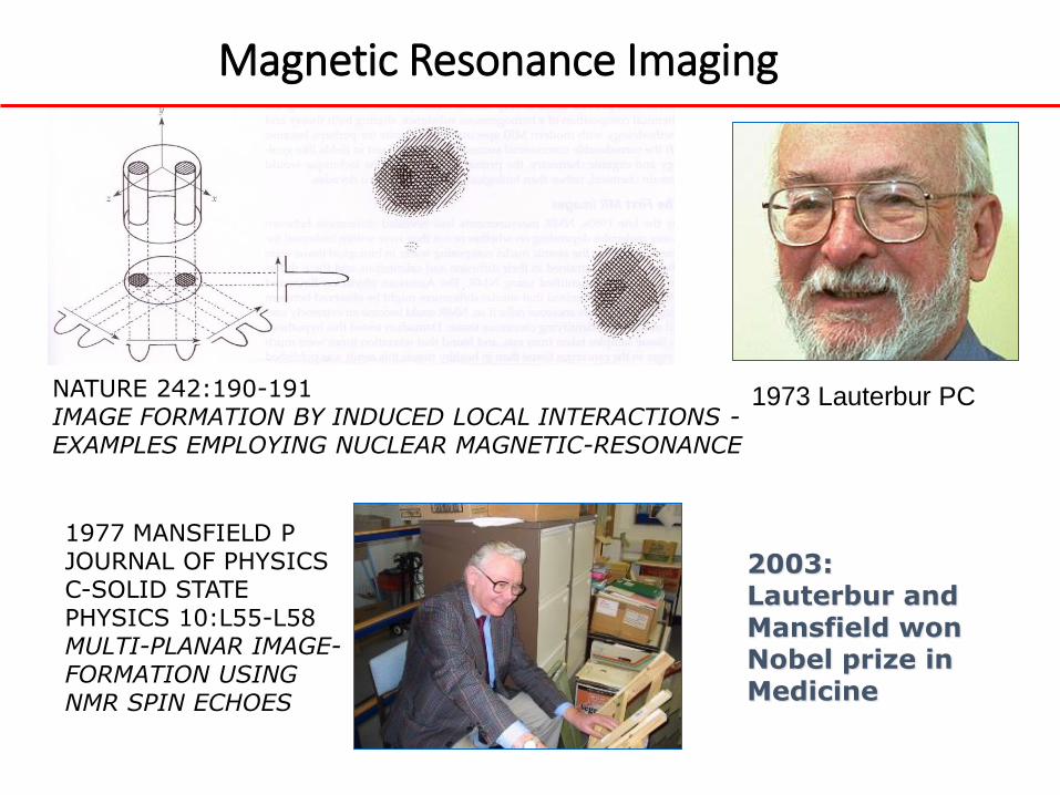
NATURE 242:190-191 IMAGE FORMATION BY INDUCED LOCAL INTERACTIONS -EXAMPLES EMPLOYING NUCLEAR MAGNETIC-RESONANCE
2003: Lauterbur and Mansfield won Nobel prize in Medicine
1977 MANSFIELD PJOURNAL OF PHYSICS C-SOLID STATE PHYSICS 10:L55-L58 MULTI-PLANAR IMAGE-FORMATION USING NMR SPIN ECHOES
1973 Lauterbur PC

Magnetic Resonance Imaging
An MR scanner consists of an electromagnet with a very strongmagnetic field (1.5 - 9.0 Tesla)
Earth’s magnetic field = 0.00005 Tesla
3 Tesla is 60,000 times stronger than the Earth’s magnetic field.

What MRI Measures
• MRI is an extremely versatile imaging modality thatcan be used to study both brain structure andbrain function.
• Both structural and functional MRI images are acquired using the same scanner.
• Different types of brain images can be generatedto emphasize contrast related to different tissuecharacteristics.

Principles of MRI
• All magnetic resonance imaging techniques rely
on a core set of physical principles.
• To understand we must begin by studying a
single atomic nuclei and illustrate its impact on
the generated MR signal.
• In particular we focus on hydrogen atoms
consisting of a single proton.

Protons can be viewed as positively charged spheres
which are always spinning. They give rise to a net
magnetic moment along the axis of the spins.
Principles of MRI

Protons can be viewed as positively charged spheres
which are always spinning. They give rise to a net
magnetic moment along the axis of the spins.
Principles of MRI
• We cannot measure the magnetization of a single
proton using MR, instead we measure the net
magnetization of all nuclei within a volume.
• The net magnetization M can be viewed as a
vector with two components.
– A longitudinal component parallel to the magnetic field.
– A transverse component perpendicular to the field.
Net Magnetization

Net Magnetization
A longitudinal component
A transverse component
an external magnetic field
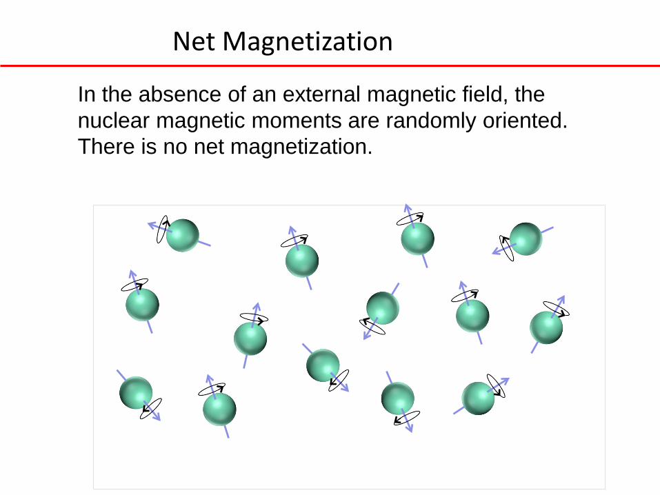
In the absence of an external magnetic field, the
nuclear magnetic moments are randomly oriented.
There is no net magnetization.
Net Magnetization

When placed in a strong magnetic field, the nuclei align
with the field. This creates a net longitudinal
magnetization in the direction of the field.
Net Magnetization
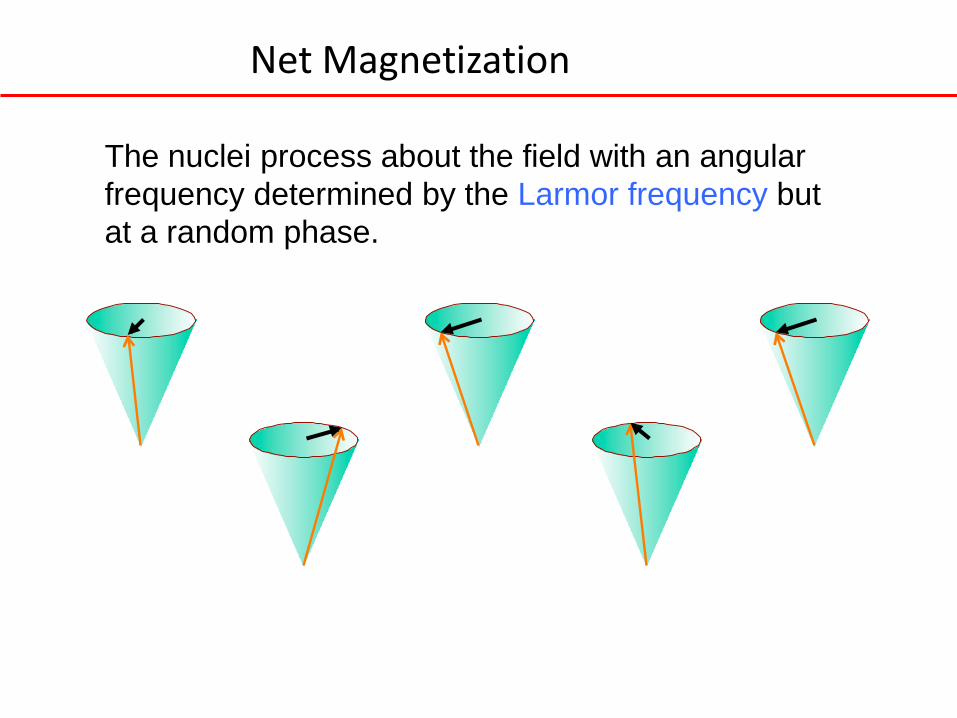
The nuclei process about the field with an angular
frequency determined by the Larmor frequency but
at a random phase.
Net Magnetization

A radio frequency (RF) pulse is used to align the
phase and ‘tip over’ the nuclei. This causes the
longitudinal magnetization to decrease, and
establishes a new transversal magnetization.
Net Magnetization

A radio frequency (RF) pulse is used to align the
phase and ‘tip over’ the nuclei. This causes the
longitudinal magnetization to decrease, and
establishes a new transversal magnetization.
Net Magnetization

• After the RF pulse is removed, the system seeks
to return to equilibrium.
• The transverse magnetization starts to disappear
(transversal relaxation),
and the longitudinal magnetization grows back
to its original size (longitudinal relaxation).
• During this process a signal is created that can
be measured using a receiver coil.
Relaxation

• Longitudinal Relaxation is the restoration of net
magnetization along the longitudinal direction as
spins return to their parallel state.
– Exponential growth described by time constant T1
• Transverse Relaxation is the loss of net
magnetization in the transverse plane due to loss
of phase coherence (resonance).
– Exponential decay described by time constant T2
Relaxation

Mz
Mo
tT1
63%
The restoration of longitudinal magnetization is
described by a time constant T1.
Longitudinal Relaxation Time

30002000100000.0
0.2
0.4
0.6
0.8
1.0
TR (msec)
Sig
na
l
white matter: T1 = 600gray matter: T1 = 1000Cerebrospinal fluid (CSF) : T1 = 3000
Longitudinal Relaxation Time

White matter and Gray matterWhite matter is a component of the central nervous system, in the brain and superficial spinal cord, and consists mostly of glial cells and myelinated axons that transmit signals from one region of the cerebrum to another and between the cerebrum and lower brain centers.
White matter tissue of the freshly cut brain appears pinkish white to the naked eye because myelin is composed largely of lipid tissue veined with capillaries. Its white color in prepared specimens is due to its usual preservation in formaldehyde.
Grey matter (or gray matter) is a major component of the central nervous system, consisting of neuronal cell bodies, neuropil (dendrites and myelinated as well as unmyelinated axons), glial cells (astroglia and oligodendrocytes) and capillaries.
Grey matter is distinguished from white matter, in that grey matter contains numerous cell bodies and relatively few myelinated axons, while white matter is composed chiefly of long-range myelinated axon tracts and contains relatively very few cell bodies.[1]
The color difference arises mainly from the whiteness of myelin. In living tissue, grey matter actually has a very light grey color with yellowish or pinkish hues, which come from capillary blood vessels and neuronal cell bodies.[2]

White matter and Gray matterWhite matter = fibers = axons which connect neurons
Grey matter (or gray matter)= neurons
CSF = something else
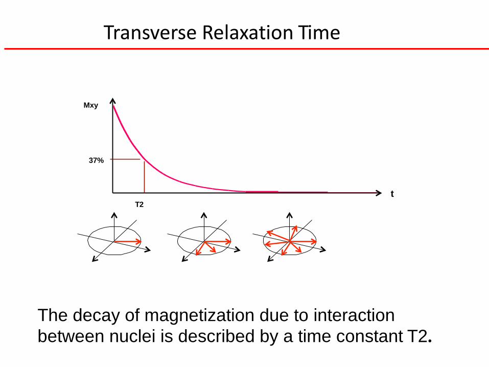
Mxy
37%
tT2
The decay of magnetization due to interaction
between nuclei is described by a time constant T2.
Transverse Relaxation Time

• By altering how often we excite the nuclei
(TR: repetition time) and how soon after
excitation we begin data collection (TE:
echo time) we can control which
characteristic is emphasized.
• The measured signal is approximately
where T1 and T2 depend tissue properties.
Image Contrast
)/exp())/exp(1( 210 TTETTRM

3. Image Formation

Image Formation
• The goal of MRI is to construct an image, or a matrix of numbers that correspond to spatial locations.
• The image depicts the spatial distribution of someproperty of the nuclei within the sample.
• This could be the density of nuclei of the tissuesin which they reside.

TR
Lo
ng
Sh
ort
Short Long
TE
ProtonDensity
T1
T2
Image Contrast
TE (echo time) -
the time between
excitation and
data collection.
)/exp())/exp(1( 210 TTETTRM

Signal Formation
• The subject is placed into the MR scanner.
– Nuclei of 1H atoms align with the magnetic field.
– The nuclei precess about the field at similar
frequencies, but at a random phase.
– Net longitudinal magnetization in the direction of field.
• Within a slice, a radio frequency (RF) pulse is used to align the phase and ‘tip over’ the nuclei.
– Causes the longitudinal magnetization to decrease,
and establishes a new transversal magnetization.
Signal Formation
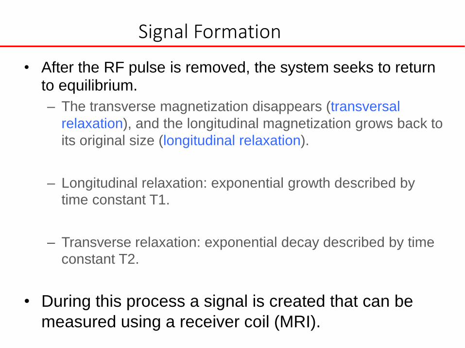
• After the RF pulse is removed, the system seeks to returnto equilibrium.
– The transverse magnetization disappears (transversal
relaxation), and the longitudinal magnetization grows back to
its original size (longitudinal relaxation).
– Longitudinal relaxation: exponential growth described by
time constant T1.
– Transverse relaxation: exponential decay described by time
constant T2.
• During this process a signal is created that can be
measured using a receiver coil (MRI).

Signal Formation

fMRI Contrast T2*
• The image we are really interested in is called
T2* image
• T2* is the combined effect of T2 and local
inhomogeneities in the magnetic field.
• The scanner can be programmed to eliminate the
effects of these inhomogeneities, or alternatively
emphasize them.
• The latter types of procedures form the basis ofBOLD fMRI (Seiji Ogawa, another Nobel prize?)

Image Contrast
• Images can be produced that are sensitive
primarily to T1, T2 (T2*).
• Because T1 vary with tissue type, it is able to
represent boundaries between CSF, gray
and white matter.
• Because T2* is sensitive to flow and
oxygenation, it is can be used to image brain
function.

T1 and T2* Images
•From now on, we will concentrate these two types of images
•T1 will tell us about the anatomy(give an example to explain the use of it?)
•T2* will tell us the activity of a specific region
(give an example to explain the use of it?)

TRTR
TE
t
…
…
T1-weightedshort TR & TE
T2-weighted
long TR & TE
T1 and T2* Images
TE TE

T1 and T2* Images
By using different sequence of (TR, TE) in experiments, we can have different images
For example:
T1 (TR= 2000 msec, TE = 20 msec) : due to different T1 for different materials (gray matter or white matter), we can read out the gray matter density in each voxel
T2* (TR=2500 msec, TE = 25 msec) : will explain a bit more in details next week
))(/exp())(/exp(1()1(
))(/exp())(/exp(1(
210
210
matterwhiteTTEmatterwhiteTTRM
mattergrayTTEmattergrayTTRMM
Intensity (percentage) of gray matter

Slice Selection
• Most structural MRI and fMRI scans involve the
construction of a three dimensional image from a
set of two-dimensional slices.

Image Formation
• Imagine a brain slice split into a number of
equally sized volume elements or voxels.
ρ(x,y)
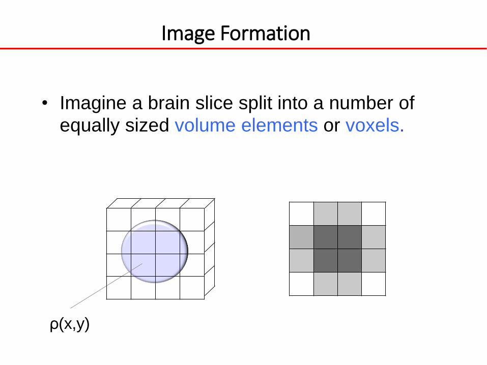
Image Formation
• Imagine a brain slice split into a number of
equally sized volume elements or voxels.
ρ(x,y)

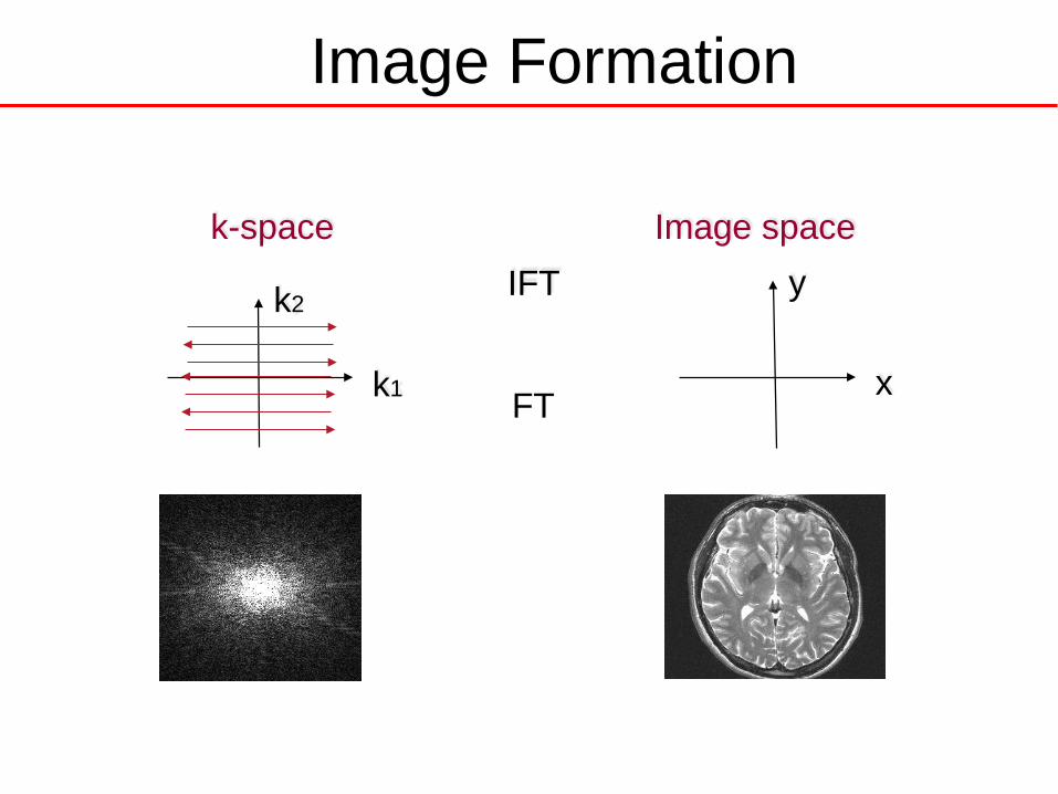
K-space
• The measurements are acquired in the
frequency-domain (k-space).

FT
IFT
k-space
k2
k1
Image space
y
x
Image Formation

K-space
• The measurements are acquired in the
frequency-domain (k-space).
• By making measurements for multiple values of
(k1, k2) we can gain enough information to
solve the inverse problem and reconstruct (x,
y).
• We can use the inverse Fourier transform (IFT):
(x, y) S(k1 ,k2 )ei2 (k1 xk2 y)
dkFdkP

K-space Measurements
• In practice, data measurements are made
discretely over a finite region.
– Use discrete Fourier transforms.
• The number of k-space measurements we make
influences the spatial resolution of the image.
– Need enough measurements to solve inverse problem.
16 unknowns 4 unknowns

4: K-space
FT
IFT
k-space
k1
k2
Image space
y
x
Image Formation

K-space
Each individual point in image space depends on all of the points contained in the k-space
It is important to note that there is not a one-to-one relationship between image and k-space.

Superposition of curves
Period: T
Frequency: =T-1
=
1 Dimension

K-space
2 Dimensions
Example

Example

Example

Example

Example

Example

Low passfilter
High passfilter
Example
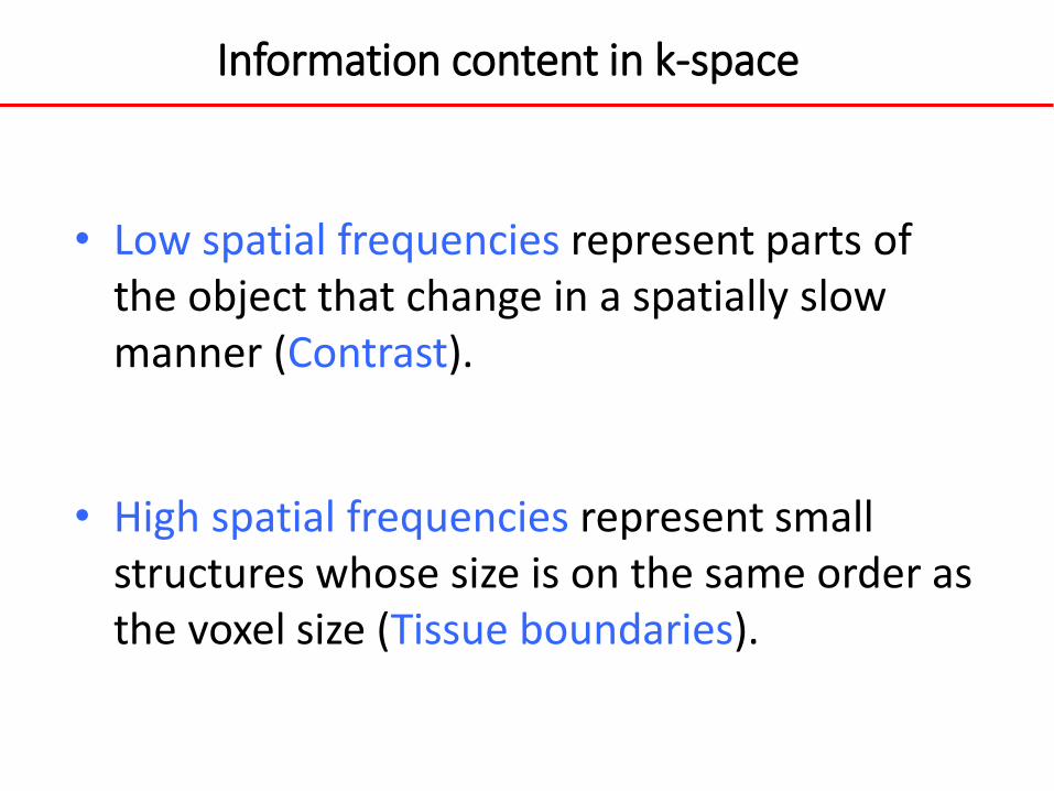
Information content in k-space
• Low spatial frequencies represent parts ofthe object that change in a spatially slowmanner (Contrast).
• High spatial frequencies represent small structures whose size is on the same order as the voxel size (Tissue boundaries).

Spatial Resolution
32 32 image
1024 points sampled in k-space
64 64 image
4096 points sampled in k-space
128 128 image
16,384 points sampled in k-space

Seminar I
Question 1. Get familiar with your matlab
Question 2. 2-D Fourier transform
For a given image h(n,m) with N columns and N rows, the FT is defined as
1) For H (k,l) = H(1,-3)=1, and 0 otherwise, work out the image of exp(- j(kn+lm)) on the (n,m) plane
1
0
1
02
1
0
1
0
),())(exp(1
),(
),())(exp(),(
N
n
N
m
N
n
N
m
lkHlmknjN
nmh
mnhlmknjlkH

2) For H(k,l) = H(7,1)=1, and 0 otherwise, work out the image of exp(- j(kn+lm)) on the (n,m) plane
Seminar I

Seminar I
• 3) load a brain image and work out its Fourier transform using fft2
• 4) play with ifft2 and see the effect of high pass and low pass filters