Computational Analysis of Piezoelectric Systems Using A ...

Computational Analysis of Piezoelectric Systems

Using A Coupled Multiphysics Finite Element Model

by

Zhiren Zhu

A thesis submitted to The Johns Hopkins University in conformity with the

requirements for the degree of Master of Science.

Baltimore, Maryland

August, 2017

c© Zhiren Zhu 2017

All rights reserved

Abstract

A multiphysics finite element model framework for coupling transient electromag-

netic and dynamic mechanical fields is utilized to perform computational analysis

of piezoelectric material systems. The model framework achieves coupling between

the mechanical and electromagnetic fields by solving the corresponding governing

equations in the time domain, and is capable of predicting the evolution of electric

field variables in a conducting medium undergoing dynamic finite deformation. The

computational model is then calibrated to reproduce experimentally-characterized be-

havior of viscoelastic piezo-nanocomposite (p-NC) structures subjected to dynamic

loading. The numerical model shows good agreement with experimental results on

the loading-frequency dependent piezoelectric output of p-NC systems. Sensitivity

study is conducted with the calibrated model to examine the effect of the mechanical

input parameters on piezoelectric output of p-NC. Based on the findings, the energy

harvesting and sensing performance of p-NC systems can be enhanced by effectively

harnessing the viscoelastic properties of the material.

Primary Reader: Professor Somnath Ghosh

Secondary Reader: Professor Sung Hoon Kang

ii

Acknowledgments

I express my gratitude to my adviser, Professor Somnath Ghosh, for sharing his

wisdom with me during my time here at Johns Hopkins. I sincerely admire his spirit

as a passionate scientist and determination to pursue perfection. It is with great pride

to claim that I learned my finite element method from Professor Ghosh.

Thanks also to Professor Sung Hoon Kang for introducing me to the world of

functional materials and the insightful discussions that gave meaning to my work. I

would also like to acknowledge the help from Jing Li during our collaborative project.

Special thanks go to Shu Guo, for kindly and patiently mentoring me, and helping

me tackle countless challenges through the course of my research. I also express

my thanks to the other fellow members of the Computational Mechanics Research

Laboratory and friends in the Department of Civil Engineering for their continued

support.

The work is supported by the Multifunctional Materials & Microsystems division

of AFOSR under award ID 2770925044895D. The sponsorship is greatly appreci-

ated. I want to also thank the staffs at Homewood High-Performance Cluster and

Maryland Advanced Research Computing Center for supporting my work with the

super-computers.

iii

Contents

Abstract ii

Acknowledgments iii

List of Tables vi

List of Figures vii

1 Introduction 1

2 Finite Element Model for Coupled Electromagnetic and Mechanical

Fields in Piezoelectric Materials 5

2.1 Governing equations for the finite deformation dynamic problem . . . 6

2.2 Governing equations for the electromagnetic problem . . . . . . . . . 10

2.3 Governing equations for the piezoelectric problem . . . . . . . . . . . 18

2.4 Finite element implementation of the coupled problem . . . . . . . . 23

2.5 Conclusion . . . . . . . . . . . . . . . . . . . . . . . . . . . . . . . . . 25

3 Analysis of Viscoelastic Piezo-nanocomposite System 26

3.1 Motivation . . . . . . . . . . . . . . . . . . . . . . . . . . . . . . . . . 26

3.2 Analytical model for piezoelectricity in viscoelastic systems . . . . . . 28

iv

CONTENTS

3.3 Calibration of computational model . . . . . . . . . . . . . . . . . . . 32

3.4 Piezoelectric performance of p-NC under dynamic large deformation . 36

3.5 Sensitivity study for optimal mechanical parameters . . . . . . . . . . 39

3.6 Conclusion . . . . . . . . . . . . . . . . . . . . . . . . . . . . . . . . . 43

4 Conclusions and Perspectives 49

Vita 63

v

List of Tables

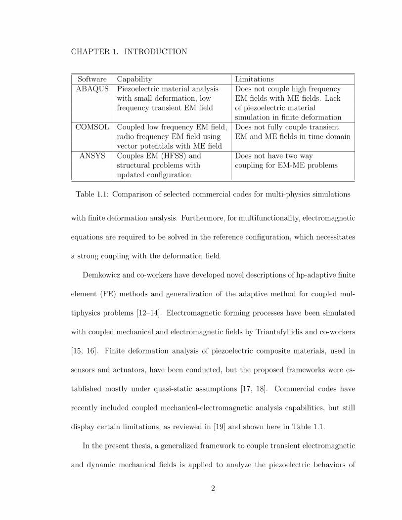
1.1 Comparison of selected commercial codes for multi-physics simulations 2

vi

List of Figures

3.1 Experimental measurement of dynamic moduli in the viscoelastic p-NC specimens: (a) comparison of storage moduli at different loadingfrequencies; (b) comparison of loss moduli at different loading frequencies. 44

3.2 Simulation results compared with experimental results for cyclic com-pression of p-NC plate. (a) 3D model and mesh of the flat plate sub-jected to cyclic compressive loading; (b) Comparison between exper-imental measurements and simulation results for peak surface chargedensity at steady-state of loading with different frequencies, on topsurface of flat plate. . . . . . . . . . . . . . . . . . . . . . . . . . . . . 45

3.3 Simulation results for p-NC models under cyclic large deformation: (a)peak magnitude of surface charge density for compressible and nearly-incompressible models of 20:1 p-NC under large cyclic deformation of10 Hz; (b),(c),(d) comparison of surface charge density time historyunder compressive and tensile cyclic loading of peak load magnitude 1kPa, 10 kPa, 100 kPa; (e),(f) Detailed view of surface charge densitytime history under compressive cyclic loading of peak load magnitude10 kPa, 100 kPa; . . . . . . . . . . . . . . . . . . . . . . . . . . . . . 46

3.4 Simulation results compared with experimental results for cyclic com-pression of curved p-NC shell. (a) Electric potential distribution inthe 3D model of a p-NC shell structure subjected to cyclic compres-sion, poled along radial direction and grounded across inner surface;(b) Comparison between experimental measurements and simulationresults for peak surface charge density at steady-state of loading withdifferent frequencies, on top surface of flat plate. . . . . . . . . . . . . 47

3.5 Results of sensitivity studies: (a) Time history of surface charge den-sity, for p-NC models with different instantaneous elastic modulus E0;(b) Dependence of viscoelastic contribution factor A(E

′

) on storagemodulus E

′

, based on experiment measurements. (c) Time history ofsurface charge density, for p-NC models with different viscous relax-ation proportion µ0; (d) Detailed comparison of steady-state surfacecharge density, for p-NC models with different viscous relaxation pro-portion µ0; (e) Time history of surface charge density, for p-NC modelswith different relaxation time τ ; (f) Detailed comparison of steady-statesurface charge density, for p-NC models with different relaxation timeτ . . . . . . . . . . . . . . . . . . . . . . . . . . . . . . . . . . . . . . 48

vii

Chapter 1

Introduction

Novel materials have recently been introduced to construct multifunctional struc-

tures governed by multiphysics principles such as the coupling of mechanical and

electromagnetic relations. The multifunctional structures are of great interest for

application in consumer electronics, structural health monitors, and aerospace struc-

tures.These structures may be active skins of aircraft [1, 2], vibration control devices

[3, 4], meta-materials for optical and communication systems [5, 6], as well as high-

mobility and stretchable electronics [7–10]. With the increased demand for the design

of multifunctional structures governed by multiphysics principles, there is a need for

robust computational code frameworks to model the coupled multiphysics problems.

Modeling framework for the evolution of electromagnetic fields in a moving de-

formable media has been under development for many decades, but the construction

of a comprehensively effective framework is still considered to be a challenging task.

Finite element analysis of electromagnetic field for signal transmission in antennas

has been traditionally carried out in the frequency domain [11]. Yet, solution process

in the frequency domain is not suitable when the electromagnetic problem is coupled

1

CHAPTER 1. INTRODUCTION

Software Capability LimitationsABAQUS Piezoelectric material analysis Does not couple high frequency

with small deformation, low EM fields with ME fields. Lackfrequency transient EM field of piezoelectric material

simulation in finite deformationCOMSOL Coupled low frequency EM field, Does not fully couple transient

radio frequency EM field using EM and ME fields in time domainvector potentials with ME field

ANSYS Couples EM (HFSS) and Does not have two waystructural problems with coupling for EM-ME problemsupdated configuration

Table 1.1: Comparison of selected commercial codes for multi-physics simulations

with finite deformation analysis. Furthermore, for multifunctionality, electromagnetic

equations are required to be solved in the reference configuration, which necessitates

a strong coupling with the deformation field.

Demkowicz and co-workers have developed novel descriptions of hp-adaptive finite

element (FE) methods and generalization of the adaptive method for coupled mul-

tiphysics problems [12–14]. Electromagnetic forming processes have been simulated

with coupled mechanical and electromagnetic fields by Triantafyllidis and co-workers

[15, 16]. Finite deformation analysis of piezoelectric composite materials, used in

sensors and actuators, have been conducted, but the proposed frameworks were es-

tablished mostly under quasi-static assumptions [17, 18]. Commercial codes have

recently included coupled mechanical-electromagnetic analysis capabilities, but still

display certain limitations, as reviewed in [19] and shown here in Table 1.1.

In the present thesis, a generalized framework to couple transient electromagnetic

and dynamic mechanical fields is applied to analyze the piezoelectric behaviors of

2


multifunctional structures. The framework is as introduced in [19, 20, 21], and suits

the need to predict the evolution of electrical and magnetic fields and their fluxes

in a vibrating substrate undergoing finite deformation. To achieve coupling between

fields with disparate frequency ranges, the governing equations are solved in the time

domain, as opposed to the frequency domain. A Lagrangian description is invoked, in

general accordance with the methods developed in [22, 23, 24]. The coupling scheme

maps Maxwell’s equations from spatial to material coordinates in the reference con-

figuration. By applying the Euler-Lagrange stationary conditions, weak forms of the

coupled dynamic mechanical and transient electromagnetic equations are generated in

the reference configuration. From the weak form, the FE equations is developed using

the Galerkin’s method. Physical variables in the Maxwell’s equations are written in

terms of a scalar potential and vector potentials, allowing for a more efficient solution

process with a reduced number of Maxwell’s equations and associated field variables.

Introduction of a gauge condition in the FE formulations helps overcome the non-

uniqueness of solutions in the reduced set of equations. Additionally, the boundary

conditions are appropriately represented in terms of the potentials, rather than the

original physical variables. Piezoelectric constitutive relations is implemented in the

framework for numerical analysis of piezoelectric materials.

Furthermore, the multiphysics FE model is applied to facilitate the characteriza-

tion and design of viscoelastic piezo-nanocomposite (p-NC) systems for energy har-

vesting and sensing applications. This class of composite materials enables the use of

3


piezoelectricity in a broad range of applications, while assuring good conversion effi-

ciency, flexibility in shape formation, and accommodation of large deformation. Since

the polymeric matrix of the piezocomposite is viscoelastic, the piezoelectric perfor-

mance of the material under dynamic loading is also expected to display frequency

dependence. Simulations were performed to calibrate the computational model and

reproduce the loading-frequency dependence of piezoelectric output measured in ex-

periments. The computational framework is further utilized to study influence of the

material model’s input mechanical parameters on the piezoelectric performance under

dynamic loading conditions.

The present thesis first reviews the formulation of the multiphysics FE framework

in Chapter 2. Governing equations for the problem is reviewed in Sections 2.1, 2.2,

and 2.3, and the FE implementation is discussed in Section 2.4. Analysis of the

viscoelastic p-NC system is introduced in Chapter 3. The thesis is concluded in

Chapter 4.

4

Chapter 2

Finite Element Model for Coupled Electro-

magnetic and Mechanical Fields in Piezo-

electric Materials

In order to evaluate the evolution of transient electromagnetic field variables in

a deformable, conducting medium undergoing finite dynamic deformation, the solu-

tion process must comprehensively couple the mechanical and electromagnetic fields

through their governing equations. Particularly in the case of piezoelectric materials,

the electromagnetic field variables depends on the deformed configuration, while the

mechanical field variables are also subjected to induced forces by the electromagnetic

field. This requires the implementation of a two-way coupling scheme to capture the

interaction between the electromagnetic and mechanical fields.

In the present framework, previously published in [19, 20], a staggered coupling

scheme is established between the electric and mechanical fields. At each time step,

the mechanical field is first solved, and the electric field is then calculated accordingly

in the updated configuration, based on the deformation solution. Information of the

5

CHAPTER 2. FE MODEL FOR COUPLED EM AND ME IN PIEZOELECTRICMATERIALS

electric field is transferred back to the mechanical field in the following time step, to

evaluate the reverse piezoelectric response.

In this chapter, the governing equations for the mechanical, electromagnetic, and

piezoelectric problems in the reference configurations and their implementation in the

FE framework are reviewed.

2.1 Governing equations for the finite deformation

dynamic problem

To model the mechanical response of the conducting medium, the FE framework

utilizes the governing equations for a hyperelastic material undergoing finite defor-

mation under dynamic loading conditions. The reference configuration Ω0 = Ω(t0) is

expressed in terms of the material coordinates XI , I = 1, 2, 3, while the current con-

figuration Ω(t) at time t is represented by the spatial coordinates xi, i = 1, 2, 3. Defor-

mation of the body is expressed using a single-valued mapping function xi = ϕi(XJ , t).

Correspondingly, the Cartesian components of the displacement vector in the material

coordinates are expressed as: ui(XJ , t) = ϕi(XJ , t)− δiJXJ .

Among the many available constitutive relations for hyperelastic material, a mod-

ified neo-Hookean material model is utilized in this study. To present the modified

neo-Hookean model, we first examine the original neo-Hookean material model, for

which the strain energy density function Ψ is expressed in terms of the kinematic

6


variables as:

Ψ =1

2λ(ln J)2 − µ ln J +

1

2µ(CII − 3) (2.1)

where µ and λ are the Lame constants, and

CIJ =∂xk

∂XI

∂xk

∂XJ

(2.2)

is the right Cauchy-Green deformation tensor, and CII is its first invariant, i.e. trace.

The positive-valued Jacobian J , which indicates volume change during deformation,

is defined in terms of the deformation gradient tensor FiJ as:

J = det(FiJ) > 0 where FiJ =∂xi

∂XJ

(2.3)

Notice that the right Cauchy-Green deformation tensor can be expressed in terms of

the deformation gradient as: CIJ = FkIFkJ .

By definition, the stress-strain relation can be derived from the energy density

expression, i.e. Equation 2.1, as:

SIJ = 2∂Ψ

∂CIJ

= λ ln JC−1

IJ + µ(δIJ − C−1

IJ ) (2.4)

For the modified version neo-Hookean model used in this study, the strain energy

density function is decomposed here into a volumetric part Ψvol(J) and a deviatoric

7


part Ψdev(CIJ) as:

Ψ(J, CIJ) = Ψvol(J) + Ψdev(CIJ) =1

2(λ+

2

3µ)(ln J)2 +

1

2µ(CII − 3) (2.5)

Here, CIJ = FkIFkJ represents the volume preserving portion of the deformation,

with FkI = J−2/3FkI , such that det FkI = 1.

Stress-strain relation can be derived for the volumetric and deviatoric parts, re-

spectively, as:

SvolIJ = 2

∂Ψvol

∂CIJ

= (λ+2

3µ) ln JC−1

IJ (2.6)

SdevIJ = 2

∂Ψdev

∂CIJ

= µJ−2/3(δIJ − 1

3C−1

IJ CKK) (2.7)

with a combined form for the overall material model as:

SIJ = SvolIJ + Sdev

IJ = (λ+2

3µ) ln JC−1

IJ + µJ−2/3(δIJ − 1

3C−1

IJ CKK) (2.8)

Addition to hyperelasticity, viscoelastic material constitutive relation is included

in order to study the viscoelastic system presented later in Chapter 3. In this case,

the second Piola-Kirchhoff stress at a given time step is expressed as:

SvolIJ = 2

∂Ψvol

∂CIJ

−QIJ (2.9)

8


where QIJ is the non-equilibrium viscous stress. The evolution of QIJ is specified by

a rate equation describing the viscoelastic material model [25, 26]:

QIJ +1

τQIJ =

(1− γ)

τdev

∂Ψ

∂EIJ

(2.10)

where τ ∈ (0,∞) is relaxation time, γ ∈ [0, 1) is a given parameter, Ψ is the deviatoric

part of the strain energy density Ψ, and EIJ is the volume-preserving part of the strain

tensor EIJ .

To obtain the formulation for finite deformation in the reference configuration, first

consider the equilibrium of a continuum body in the current deformed configuration:

∂tσij

∂txj

+t ρbi =t ρui (2.11)

where tσij = J−1FiKFjLSKL is the Cauchy stress in the current configuration, bi

is the body force per unit volume, tρ is the density of the deformed material. It is

worthwhile to note that the density of the undeformed material is written as 0ρ = J tρ.

With the principle of virtual work and applying the divergence theorem, we may

express the weak form as:

∫ t

tV

σij∂δui

∂txj

dtV +

∫ t

tV

ρuiδuidtV =

∫ t

tS

σijδutinjd

tS +

∫ t

tV

ρbiδuidtV (2.12)

Note that the integration domain is the current configuration. In order to solve the

9


problem, the formulation is mapped to the reference configuration. Here, we can use

relationships from mass conservation:

0ρ = J tρ dtV = Jd0V s.t. 0ρd0V =t ρdtV (2.13)

to rewrite the weak form as:

∫

0V

t0PiJ +

∫

0V

0ρuiδuid0V =

∫

0S

t0PiJδuiNJd

0S +

∫

0V

0ρbiδuid0V (2.14)

where t0PiJ = J tσikF

−1

Jk = ∂xi

∂XK

t

0SKJ is the first Piola-Kirchhoff stress. This allows for

the equilibrium condition at t = 0 in the reference configuration to be expressed as:

∂t0PiJ

∂XJ

+ 0ρbi =0ρui (2.15)

2.2 Governing equations for the electromagnetic

problem

The governing equations for the electromagnetic problem is based on the conventional

Maxwell’s equations for a conducting medium. These equations are expressed in the

10


current configurations in terms of the current coordinate xi(t) as:

di,i = qe Gauss’ law of electricity (2.16a)

bi,i = 0 Gauss’ law of magnetism (2.16b)

εijkek,j = −∂bi∂t

Faraday’s law of magnetism (2.16c)

εijkhk,j =∂di∂t

+ jfi Ampere’s law (2.16d)

Here di is the Cartesian components of the electrical displacement field vector, qe is

free charge density, bi are the components of the magnetic induction field vector, ei is

electric field vector, hi is the magnetic field strength vector, and jfi is the free charge

current defined as:

jfi , jci + qexi (2.17)

where jci is conducting current and εijk is the Levi-Civita permutation symbol. In

the absence of magnetization and polarization, the constitutive laws for an isotropic

material in the current configuration are given as:

di = εei (2.18a)

hi =1

µbi (2.18b)

jci = σ(ei + εijkxjbk) (2.18c)

where permittivity ε, permeability µ, and conductivity σ are material constants.

11


In order to achieve coupling with the set of mechanical field equations, the Maxwell’s

equations must be represented in the reference configuration Ω0. Following the deriva-

tion presented in [19, 21], we may arrive at the following form:

DI ,I = Qe (2.19a)

BJ ,J = 0 (2.19b)

εIJK∂

∂XJ

EK = − d

dtBI (2.19c)

εIJK∂

∂XJ

HK =d

dtDI + J c

I (2.19d)

Note that the electric and magnetic induction fields in the reference configuration is

defined as:

EI , [ej − εjmn(bmxn)]xj,I (2.20a)

BJ , JXJ,ibi (2.20b)

12


and the constitutive laws in the reference configuration are expressed as:

DI = εJXI ,j XJ ,j [EJ + εJKL(∂XK

∂tBL)] = εJC−1

IJ [EJ + εJKL(∂XK

∂tBL)] (2.21a)

HJ = hixi,J +εJKL∂XK

∂tDL

=1

µJ−1xi,M xi,J BM + εJKL

∂XK

∂t

εJC−1

LN [EN + εNPQ(∂XP

∂tBQ)]

=1

µJ−1CMJBM + εJKL

∂XK

∂t

εJC−1

LN [EN + εNPQ(∂XP

∂tBQ)]

(2.21b)

J cI = σJC−1

IJ EJ (2.21c)

Instead of directly solving the variables in the Maxwell’s equations, the present

framework proposes a scalar potential ϕ for the electric field and a vector potential

a for the magnetic field, in the current configuration, as primary variables. This ap-

proach was followed by Nelson in [27], and effectively reduces the Maxwell’s equations

from four to two independent equations.

Given that the divergence of the magnetic induction vector b is zero, the magnetic

vector potential a is derived using a vector identity:

∇ · b = ∇ · (∇× a) = 0 =⇒ bi = εijkak,j (2.22)

This allows for the Faraday’s law in the current configuration, i.e. Equation 2.16c, to

be expressed as:

εijk(ek + ak),j = 0 (2.23)

13


Since the curl of gradient of any scalar field is a null vector, the gradient of ε is placed

in the LHS to yield the form:

εijk(ek + ak + ε,k),j = 0 (2.24)

allowing for the expression of electric field using the mixed potentials:

ek = −ϕ,k − ak (2.25)

Introduction of the potentials in the Gauss’ law of magnetism of Equation 2.16b

results in identity. The remaining Maxwell’s equations are reformulated as:

∇2ϕ+∂

∂t(ai,i) = −qe (2.26a)

(∇2ai − µε∂2ai∂t2

)− (ak,k + µε∂ϕ

∂t),i = −µji (2.26b)

To obtain a corresponding reduced form of the Maxwell’s equations in the reference

configuration, the potentials is defined with the transformation functions as:

Φ = ϕ− dxi

dtai (2.27a)

AK = aixi,K (2.27b)

In the reference configuration, the electric and magnetic induction fields can be

14


written in terms of the mixed potentials as:

EI = −Φ,J − ∂AI

∂t(2.28a)

BI = εIJKAK,J (2.28b)

which can be substituted to the Maxwell’s Equations 2.19a and 2.19d to generate the

governing equations:

(

εJC−1

IJ EJ

)

,I = Qe (2.29a)

εIJK

(1

µJCKLεLMNAN,M + εKPQ

∂XP

∂tεJC−1

QRER

)

,J =d

dtεJC−1

IP EP

+ σJC−1

IQ

(

−Φ,Q −AQ

)

(2.29b)

where EI is defined as:

EI = EI + εIJK∂XJ

∂tBK = −Φ,I −AI + εIJK

∂XJ

∂tεKMNAN,M (2.30)

Although the reduced representation of Maxwell’s equations is advantageous com-

putationally, it also leads to non-uniqueness of solution for certain state of the EM

fields. Therefore, the Coulomb gauge condition is enforced, as proposed in [18, 28, 29],

to avert the non-uniqueness. This condition is states as:

AI,I = 0 (2.31)

15


which implies a restriction to the irrotational term in Equation 2.28b.

The weak form of the transient electromagnetic problem is derived using the

Hamilton’s principle [22, 27]. By minimizing the action functional S over the time

range t1 to t2, which is defined in terms of the time-dependent Lagrangian density L

in the reference domain:

δS = δ

∫ t2

t1

∫

Ω0

LdΩ0dt = 0 (2.32)

where the Lagrangian density in the reference and current configuration, L and l

respectively, are given as:

L = Jl = (ε

2eiei −

1

2µbjbj + jkak − qϕ) (2.33)

and can be expressed in terms of the scalar and vector potentials in the reference

configuration as:

L =εJ

2C−1

JKEJEK − J−1

2µ(CLMBLBM) + JNAN −QΦ (2.34)

Furthermore, the gauge condition is implemented using a penalty method to constrain

the vector potential, following [28,18,29]. This adds an additional term 1

p(∇ ·A)2 to

the Lagrangian density function:

L =εJ

2C−1

JKEJEK − J−1

2µ(CLMBLBM) + JNAN −QΦ +

1

p(AP,P )

2 (2.35)

16


The penalty coefficient 1/p is usually of the order of the electric permittivity ε.

Setting the variation of S with respect to Φ and A to be zero, we obtain:

S,Φ[δΦ] =

∫ t2

t1

∫

Ω0

L,Φ[δΦ]Ω0dt = 0 (2.36a)

S,Φ[δA] =

∫ t2

t1

∫

Ω0

L,A[δA]Ω0dt = 0 (2.36b)

Given arbitrary t1 and t2, the above leads to:

∫

Ω0

L,Φ [δΦ]dV0 =

∫

∂Ω0

NI

(

εJC−1

IJ EJδΦ)

dS0 −∫

Ω0

(

εJC−1

IJ EJ −Q)

δΦ,I dV0 = 0

(2.37a)∫

Ω0

L,A [δA]dV0 =

∫

∂Ω0

NL(εKLMQMδAK)dS0 −2

p

∫

∂Ω0

AR,R NKδAKdS0+

∫

Ω0

εSPRQP∂

∂XR

δASdV0 −∫

Ω0

d

dtεJC−1

KJEJδAKdV0 −∫

Ω0

σJC−1

KIEIδAKdV0+

2

p

∫

Ω0

AR,R δAK ,K dV0 = 0

(2.37b)

with the condensed term expressed as:

QM =1

µJCMNBN + εMNP

∂XN

∂tεJC−1

PQEQ (2.38)

17


2.3 Governing equations for the piezoelectric prob-

lem

The piezoelectric effect is commonly analyzed and studied under small deformation

setting due to its natural properties. Common examples of piezoelectric materials

include crystals and ceramics, which can be adequately analyzed with the elastic

constitutive equations of small deformation. The electric field is also calculated in

the same configuration. A set of constitutive relations is well established for this class

of materials [27, 30–32], and will be first reviewed here.

The canonical electro-mechanical power per unit volume of the continuum is,

e = σij εij + ekdk (2.39)

where e is the internal energy density, σij is the Cauchy stress, εij = (ui,j + uj,i)/2

is the infinitesimal strain tensor from displacement ui, dk is the electric displacement

field, and ek = φ,k is the electric field derived from electric potential.

Following the formulation by Nelson in [27], define electric enthalpy density h for

small deformation:

h = e− eidi (2.40)

18


which can be combined with Equation 2.39 to obtain:

h = σij εij − diei (2.41)

Noticing the implication that h is a function of strain εij and electric field ek, propose

the functional form:

h =1

2CE

ijklεklεij −1

2εSijejei − eimnεmnei (2.42)

which yields the expressions for Cauchy stress σij and electric displacement di:

σij =∂h

∂εij= CE

ijklεkl − ekijek (2.43)

di =∂h

∂ei= eimnεmn = εSijej (2.44)

Then, from Equations 2.40 and 2.42, we express the stored energy as:

e =1

2CE

ijklεklεij +1

2εSijejei (2.45)

Although this set of constitutive equations is not the only form developed for piezo-

electric materials, as shown by Nelson in [27], it is widely employed and therefore

selected suitable for our model framework.

In order to study piezoelectricity under finite deformation, it is necessary to de-

19


velop a Lagrangian description. This can be achieved based on the general form of

Maxwell’s equations presented in the previous section. For the case of piezoelectric

application, free charge Qe and conducting current JeI do not exist in the material,

and the magnetic field has negligible effect on the electric field. This allows for the

governing equations to be reduced to the following form:

DI ,I = 0 (2.46a)

BJ ,J = 0 (2.46b)

εIJK∂

∂XJ

EK = 0 (2.46c)

εIJK∂

∂XJ

HK =d

dtDI (2.46d)

By Poynting’s theorem, multiple EI on both sides of Equation 2.46d and subtract the

product of Equation 2.46c multiplied by HI on both sides, then using the identity

− (εIJKEJHK) ,I = EIεIJK∂

∂XJ

HK−HIεIJK∂

∂XJ

EK , the following relation is obtained:

−(εIJKEJHK),I = EIDI (2.47)

which can be integrated over the reference configuration, and then applied divergence

theorem to obtain:

∫

∂Ω0

−εIJKEJHKNIdS0 =

∫

Ω0

EIDIdV0 (2.48)

20


The LHS of the above equation is the flux of electromagnetic energy leaving the system

from the boundary, while the RHS represents the rate of change in the electromagnetic

energy of the system. This establishes the energy balance of the system.

Following derivation framework presented by Holzapfel in [33], a strong form of

Clausius-Planck inequality for the piezoelectric system can be obtained based on the

laws of thermodynamics:

Dint = EIDI + SIJEIJ − e+Θη ≥ 0 (2.49)

where Dint is the internal dissipation of the system, Θ is absolute temperature, and

η is entropy per unit volume. Detail of the derivation process can be found in [21].

By defining Helmholtz free energy as:

Ψ = e−Θη (2.50)

Equation 2.49 can be rewritten as:

Dint = EIDI + SIJEIJ − Ψ + ηΘ ≥ 0 (2.51)

When there is no internal dissipation, i.e. Dint = 0, and thermal effect is ignored, the

following equality holds:

EIDI + SIJEIJ − Ψ = 0 (2.52)

21


Furthermore, using Legendre transformation, define electric enthalpy density in

the reference configuration as:

H = Ψ− EIDI (2.53)

Taking time derivative of the electric enthalpy density, the following relation is ob-

tained upon manipulations:

H = SJKEJK − EIDI (2.54)

which gives the generalized constitutive relationship for piezoelectric material:

SIJ =∂H∂EIJ

(2.55)

DK =∂H∂EK

(2.56)

In the piezoelectric system, the coupling between mechanical and electric fields

is achieved by a piezoelectric constant EKIJ . Following the form of electric enthalpy

density in the current configuration, as presented in Equation 2.42, a form for the

electric enthalpy density in the reference configuration is proposed as:

H = ΨME(CIJ)− EKIJEIJEK − 1

2εJC−1

IJ EIEJ (2.57)

22


where ΨME(CIJ) is the stored energy density for the hyperelastic material model.

Substituting this proposed form into Equations 2.55 and 2.56, respectively, the full

expression for the second Piola-Kirchhoff stress SIJ and electric displacement DK is

obtained:

SIJ =∂H∂EIJ

=∂ΨME

∂EIJ︸︷︷︸

SME

IJ

− EKIJEK︸︷︷︸

SPiezo

IJ

− 1

2εJ

[(EPC

−1

PQEQ

)C−1

IJ − EpEQ

(C−1

PIC−1

JQ + C−1

PJC−1

IQ

)]

︸︷︷︸

SMaxwell

IJ

(2.58)

DK = − ∂H∂EK

= EKIJEIJ + εJC−1

LKEL (2.59)

2.4 Finite element implementation of the coupled

problem

For the coupled mechanical-electromagnetic problem, numerical implementation of

the weak forms is conducted with a staggered approach, where the dynamic dis-

placement field is solved first, followed by the electromagnetic problem. The semi-

discretization method involving separation of variables is used to represent the vari-

ables as discrete functions of space, while being continuous functions of time.

In the case of 8-noded brick elements, as implemented in the present framework,

independent variables, viz. displacements, scalar potential, and vector potential,

23


within each element e are interpolated as:

ue(X, t) ≈8∑

α=1

ueα(t)N

eα(X) (2.60a)

Φe(X, t) ≈8∑

α=1

Φeα(t)N

eα(X) (2.60b)

Ae(X, t) ≈8∑

α=1

Aeα(t)N

eα(X) (2.60c)

where N(X) are the trilinear isoparametric shape functions of the brick element [34].

It must be noted that the same finite element mesh is used for the solutions of mechan-

ical and electromagnetic field variables. The implicit time integration Newmark-beta

method, which assumes constant average acceleration in each time step [35, 36], is

implemented here for time integration in the dynamic mechanical problem. For the

electromagnetic field, a backward Euler method is implemented [19, 37].

For efficient computation of the large degrees of freedom (DOF) problems, the

finite element code is parallelized using available libraries. The ParMETIS library

[38] is utilized to decompose the computational domain and distribute to multiple

processors. Subsequently, parallelization of the code is accomplished by employing

the Portable Extensible Toolkit for Scientific Computation (PETSC) library [39], a

Message Passing Interface (MPI) based library.

24


2.5 Conclusion

A finite element framework that couples finite deformation dynamic problems with

transient electromagnetic problems is reviewed in this chapter. To examine the effect

of material deformation on the electromagnetic field variables, reference configura-

tion formulation of the governing equations is developed, and weak forms for the

mechanical and electromagnetic problems are constructed. Additionally, piezoelec-

tric material relation is incorporated for analysis of two-way coupling between the

mechanical and electromagnetic fields. With the established framework, evolution of

electric field in a piezoelectric material undergoing dynamic finite deformation can be

analyzed.

25

Chapter 3

Analysis of Viscoelastic Piezo-nanocomposite

System

Polymer-based piezoelectric nanocomposite (p-NC), made of polymeric matrix

and piezoelectric particles with conductive additives, is a class of materials that en-

ables the use of piezoelectricity in a broad range of applications. Since the polymeric

matrix is viscoelastic, it is expected that the piezoelectric performance of the material

under dynamic loading displays frequency dependence. In this chapter, an analytical

model describing piezoelectric behavior of viscoelastic systems is presented, and sim-

ulations were performed with the multiphysics FE model to predict the evolution of

electric field in the p-NC systems undergoing finite deformation.

3.1 Motivation

There has been a continuously growing interest in the use of nanogenerators for sus-

tainable and portable power applications through harvesting of mechanical energy.

Active research has been conducted to utilize devices made of piezoelectric mate-

rials as power sources for wearable electronics [40, 41], healthcare devices [42, 43],

26

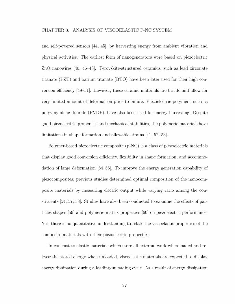
CHAPTER 3. ANALYSIS OF VISCOELASTIC P-NC SYSTEM

and self-powered sensors [44, 45], by harvesting energy from ambient vibration and

physical activities. The earliest form of nanogenerators were based on piezoelectric

ZnO nanowires [40, 46–48]. Perovskite-structured ceramics, such as lead zirconate

titanate (PZT) and barium titanate (BTO) have been later used for their high con-

version efficiency [49–51]. However, these ceramic materials are brittle and allow for

very limited amount of deformation prior to failure. Piezoelectric polymers, such as

polyvinylidene fluoride (PVDF), have also been used for energy harvesting. Despite

good piezoelectric properties and mechanical stabilities, the polymeric materials have

limitations in shape formation and allowable strains [41, 52, 53].

Polymer-based piezoelectric composite (p-NC) is a class of piezoelectric materials

that display good conversion efficiency, flexibility in shape formation, and accommo-

dation of large deformation [54–56]. To improve the energy generation capability of

piezocomposites, previous studies determined optimal composition of the nanocom-

posite materials by measuring electric output while varying ratio among the con-

stituents [54, 57, 58]. Studies have also been conducted to examine the effects of par-

ticles shapes [59] and polymeric matrix properties [60] on piezoelectric performance.

Yet, there is no quantitative understanding to relate the viscoelastic properties of the

composite materials with their piezoelectric properties.

In contrast to elastic materials which store all external work when loaded and re-

lease the stored energy when unloaded, viscoelastic materials are expected to display

energy dissipation during a loading-unloading cycle. As a result of energy dissipation

27


in viscoelastic material, a reduced amount of mechanical energy is ultimately con-

verted to piezoelectric particles. Therefore, it is critical to harness the viscoelastic

properties of the p-NC system to further enhance piezoelectric performance.

3.2 Analytical model for piezoelectricity in viscoelas-

tic systems

An analytical model is proposed to describe the frequency-dependence of piezoelectric

performance in a viscoelastic system. Consider a thin plate of p-NC subjected to

uniaxial compression. During the deformation process of the viscoelastic p-NC, part

of the total work is dissipated as heat through viscous loss, while the remaining

energy is stored as elastic strain energy. The stored elastic energy is then transferred

to electrical energy. The total work input to the piezoelectric particles, Wpiezo, can

thus be written as

Wpiezo = Vpiezo(US − UD) (3.1)

where Vpiezo is the volume of the piezoelectric particles, while US and UD are the

stored and dissipated energy density, respectively. Here, it is assumed that the p-NC

is transversely isotropic with a polarization direction normal to the loaded surface.

In terms of the output electric field E , the electrical energy density, Ue, may be

expressed as

Ue =1

2εpiezo|E|2 (3.2)

28


where εpiezo is permittivity of the piezoelectric particle. When electric charges are

generated by the piezoelectric particles, the total electric potential energy, We, is

We = V Ue =1

2V εpiezo|E|2 (3.3)

where V is the total volume of the p-NC material.

Since the electric potential energy is generated from the mechanical energy applied

to the piezoelectric particles, we may assume that the converted electrical energy is

equal to the work input, i.e. We = Wpiezo. This allows for the magnitude of the

output electric field to be written as

|E| =√

2Vpiezo(US − UD)

V εpiezo(3.4)

Piezoelectric coefficient, dij, is commonly used to quantify the charge generation

due to application of stress, and this evaluated by the relation

dij =ρiσj

(3.5)

where ρi is the charge density corresponding to induced electric field in the i direction

and σj is applied stress in the j direction, where a Kelvin notation system is employed

to express the stress tensor components. For example, in the case where the material

is polarized along the “3” direction, d33 indicates the charge density along the po-

29


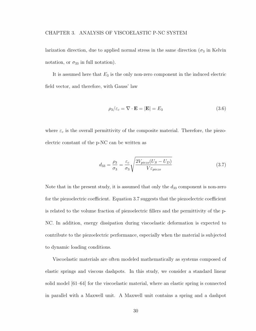
larization direction, due to applied normal stress in the same direction (σ3 in Kelvin

notation, or σ33 in full notation).

It is assumed here that E3 is the only non-zero component in the induced electric

field vector, and therefore, with Gauss’ law

ρ3/εc = ∇ · E = |E| = E3 (3.6)

where εc is the overall permittivity of the composite material. Therefore, the piezo-

electric constant of the p-NC can be written as

d33 =ρ3σ3

=εcσ3

√

2Vpiezo(US − UD)

V εpiezo(3.7)

Note that in the present study, it is assumed that only the d33 component is non-zero

for the piezoelectric coefficient. Equation 3.7 suggests that the piezoelectric coefficient

is related to the volume fraction of piezoelectric fillers and the permittivity of the p-

NC. In addition, energy dissipation during viscoelastic deformation is expected to

contribute to the piezoelectric performance, especially when the material is subjected

to dynamic loading conditions.

Viscoelastic materials are often modeled mathematically as systems composed of

elastic springs and viscous dashpots. In this study, we consider a standard linear

solid model [61–64] for the viscoelastic material, where an elastic spring is connected

in parallel with a Maxwell unit. A Maxwell unit contains a spring and a dashpot

30


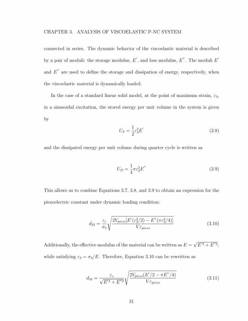
connected in series. The dynamic behavior of the viscoelastic material is described

by a pair of moduli: the storage modulus, E′

, and loss modulus, E′′

. The moduli E′

and E′′

are used to define the storage and dissipation of energy, respectively, when

the viscoelastic material is dynamically loaded.

In the case of a standard linear solid model, at the point of maximum strain, ε3,

in a sinusoidal excitation, the stored energy per unit volume in the system is given

by

US =1

2ε23E

′

(3.8)

and the dissipated energy per unit volume during quarter cycle is written as

UD =1

4πε2

3E

′′

(3.9)

This allows us to combine Equations 3.7, 3.8, and 3.9 to obtain an expression for the

piezoelectric constant under dynamic loading condition:

d33 =εcσ3

√

2Vpiezo[E′(ε2

3/2)− E ′′(πε2

3/4)]

V εpiezo(3.10)

Additionally, the effective modulus of the material can be written as E =√E ′2 + E ′′2,

while satisfying ε3 = σ3/E. Therefore, Equation 3.10 can be rewritten as

d33 =εc√

E ′2 + E ′′2

√

2Vpiezo(E′/2− πE ′′/4)

V εpiezo(3.11)

31


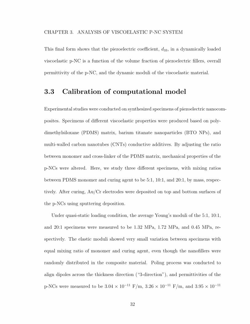
This final form shows that the piezoelectric coefficient, d33, in a dynamically loaded

viscoelastic p-NC is a function of the volume fraction of piezoelectric fillers, overall

permittivity of the p-NC, and the dynamic moduli of the viscoelastic material.

3.3 Calibration of computational model

Experimental studies were conducted on synthesized specimens of piezoelectric nanocom-

posites. Specimens of different viscoelastic properties were produced based on poly-

dimethylsiloxane (PDMS) matrix, barium titanate nanoparticles (BTO NPs), and

multi-walled carbon nanotubes (CNTs) conductive additives. By adjusting the ratio

between monomer and cross-linker of the PDMS matrix, mechanical properties of the

p-NCs were altered. Here, we study three different specimens, with mixing ratios

between PDMS monomer and curing agent to be 5:1, 10:1, and 20:1, by mass, respec-

tively. After curing, Au/Cr electrodes were deposited on top and bottom surfaces of

the p-NCs using sputtering deposition.

Under quasi-static loading condition, the average Young’s moduli of the 5:1, 10:1,

and 20:1 specimens were measured to be 1.32 MPa, 1.72 MPa, and 0.45 MPa, re-

spectively. The elastic moduli showed very small variation between specimens with

equal mixing ratio of monomer and curing agent, even though the nanofillers were

randomly distributed in the composite material. Poling process was conducted to

align dipoles across the thickness direction (“3-direction”), and permittivities of the

p-NCs were measured to be 3.04 × 10−11 F/m, 3.26 × 10−11 F/m, and 3.95 × 10−11

32


F/m for the 5:1, 10:1, and 20:1 specimens, respectively. Larger portion of PDMS

monomer corresponded to higher dielectric constant.

The storage and loss moduli of the prepared p-NCs were measured with dynamic

mechanical analyzer (DMA, TA Instruments TA Q800) at a constant strain of 0.5%.

As functions of loading frequency, the dynamic moduli of the p-NCs are shown in

Figure 3.1. Additionally, the dielectric constant of the p-NC was measured as a

function of frequency. It was found that for each of the three types of p-NC specimens

tested, the dielectric constant remain constant at the loading frequency range of 1 to

100 Hz studied.

A piezoelectric dynamic measurement setup was constructed to characterize the

piezoelectric performance of the p-NCs under dynamic loading conditions. A mini-

shaker was used to apply cyclic loading to the p-NCs, while the generated loads

were monitored by a load cell (LRM200, 10 lb, Futek). As the p-NC is compressed

by the applied loading, piezoelectric potential is generated across its thickness. The

generated electrical charges were measured by a combination of charge amplifier (piezo

film lab amplifier, TE Connectivity) and an oscilloscope (TDS2024B, Tektronix). At

each loading frequency, the peak surface charge density during the cyclic loading was

monitored to evaluate the piezoelectric performance, as shown in Figure 3.2b.

Utilizing the multiphysics FE framework, a computational model for the p-NC

material is then calibrated to reproduce the dependence of piezoelectric performance

on loading frequency, and allow for extensive studies to determine an optimal set of

33


mechanical parameters for the p-NC.

The uniaxial cyclic compression tests of the 20:1, 10:1 and 5:1 p-NCs were first

simulated, in which the steady-state peak output surface charge density values were

compared with the experimental measurements. At each loading frequency, the piezo-

electric coefficient of the material was determined according to the analytical model

of Equation 3.11, while the storage and loss moduli are the DMA-measured values

shown in Figure 3.1. In the FE framework, viscoelastic behavior of material is de-

scribed by a pair of mechanical parameters, instantaneous modulus modulus E0 and

viscous relaxation term µ0. The parameters are calibrated to satisfy the following

two conditions:

E∞ = E0(1− µ0) (3.12)

E′

(ω) = E∞ + E0µ0

(ωτ)2

1 + (ωτ)2(3.13)

where ω is the angular frequency of the applied loading, E∞ is the equilibrium long-

term elastic modulus determined by the quasi-static loading tests, and E′

(ω) and

τ are the storage modulus and relaxation time determined by the dynamic loading

tests.

The 3D mesh and boundary conditions of the model are depicted in Figure 3.2a.

The plate was grounded at the bottom surface by setting its electric potential to

φ = 0, and uniform cyclic compression was applied on the top surface, with traction

34


magnitude described by

T (t) =Tp

2[1 + sin(ωt− π

2)] (3.14)

where Tp is the maximum prescribed compression in the cyclic loading process, set

to be Tp = 400 Pa here, equal to the peak load applied in the dynamic compression

experiment.

Difference of electric potential ∆φ across the thickness of the plate was monitored,

and peak value at steady-state, ∆φp(Tp, ω), was recorded to compute the peak surface

charge density ρp(Tp, ω) according to the relation

ρp(Tp, ω) =ε0εrd

∆φp(Tp, ω) (3.15)

where d is the plate thickness, ε0 = 8.85 × 10−12 F·m−1 is the vacuum permittivity,

and εr is the relative permittivity of the material. The FE predictions of ρp(Tp, ω) are

compared with experiment results in Figure 3.2b. As observed, the FE model with

the calibrated material parameters is able to capture the piezoelectric behavior in the

p-NCs under uniaxial cyclic compression and reproduce the relation between loading

frequency and peak steady-state charge output. In the range of investigated applied

loading frequency, the increase of loading frequency corresponded to a decrease of peak

piezoelectric output, at a constant value of peak load. This result again confirms

that the viscoelasticity of the composite material affects the dynamic piezoelectric

performance of p-NC systems.

35


3.4 Piezoelectric performance of p-NC under dy-

namic large deformation

Since a major advantage of the p-NC is its accommodation of large deformation, it

is of great interest to investigate the piezoelectric performance of the material under

dynamic large deformation. Simulations were performed on uniaxial cyclic tension

and compression of the 20:1 p-NC material model (quasi-static modulus E∞ = 450

kPa) at a frequency of 10Hz. Here, peak loading values of Tp = ±1 kPa, ±10 kPa,

and ±100 kPa were examined, with the loading pattern described by Equation 3.14.

The applied loading values in the latter sets are sufficient for large deformation to

occur in the material. Additionally, the same set of simulations were performed on a

modified material model with Poisson’s ratio of ν = 0.30 and other input parameters,

viz. E0, µ0, τ , d33, and εr, assumed to be unchanged. The original material model,

calibrated earlier according to the experiment measurement, is nearly-incompressible,

with Poissons ratio set as ν = 0.499.

The measured peak magnitude of surface charge density in the aforementioned

cases and the time histories of surface charge density are shown in Figure 3.3. It is

observed that, given an equal magnitude of peak load |Tp|, cyclic tension produces a

higher output charge density than is produced by cyclic compression, and the advan-

tage of applying cyclic tension is more profound when |Tp| is high and also when the

material is nearly incompressible. For the compressible material model (ν = 0.30),

36


the electric field generated under cyclic tension and compression are in opposite di-

rections, which can be noticed from the time history of output charge in Figures 3.3b,

3.3c and 3.3d. However, this is not the case for the nearly-incompressible material

model (ν = 0.499). When the nearly-incompressible material is subjected to cyclic

compression of relatively large peak load, the direction of piezoelectric field is in the

same direction as that generated by cyclic tension.

To explain this phenomenon, consider a perfectly incompressible material with

ν = 0.5, also poled to have a piezoelectric strain coefficient d33. This results in the

non-zero piezoelectric stress coefficients e31 = e32 = λd33 and e33 = (λ + 2µ)d33,

where λ and µ are the Lame constants. Note that, in full notation, the piezoelectric

stress coefficient eijk is related to the piezoelectric strain coefficient dimn through the

relation [31]:

eijk = dimnCmnjk (3.16)

where Cmnjk is the elasticity stiffness tensor.

From this, we can deduce e31/e33 = ν/(1− ν), and when ν = 0.5, e31 = e32 = e33.

That is, the piezoelectric contribution from a unit principal strain in the loading

direction and that from a unit principal strain in the transverse direction are equal

in an incompressible material.

In the case of pure tension or compression, the Green-Lagrange strain tensor

has the non-zero components E11 = E22 = (1/α − 1)/2 and E33 = (α2 − 1)/2,

where α = α3 is the principal stretch along the loading direction. It can be seen

37


that E11 + E22 + E33 ≥ 0 always holds, with E11 + E22 + E33 = 0 satisfied only at

α = 1, i.e. no deformation. For a perfectly incompressible material, we thus expect

the generated electric field to be always in the same direction when the material is

subjected to uniaxial tension and compression. In the nearly incompressible case

studied, since Poissons ratio is slightly below 0.5, the piezoelectric coefficient e33 is

slightly larger than e31 and e32. As a result, when the material is subjected to a

small amount of uniaxial compression, the contribution of E33 to the electric field is

still stronger than the total contribution by E11 and E33, as observed in Figure 3.3b.

When the material is further deformed, the generated electric field switches direction,

as seen in Figures 3.3c and 3.3d. This suggests that, by adjusting the compressibility

of the p-NC material, we can control the possible direction of the piezoelectric field

generated under large deformation.

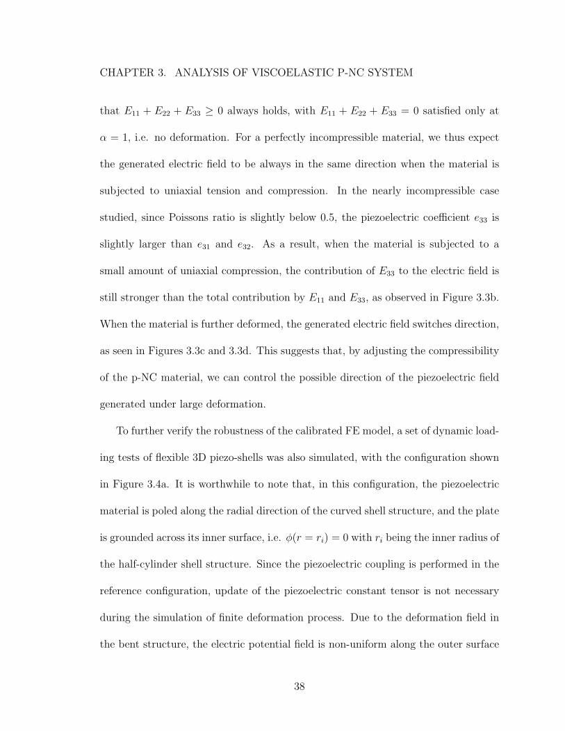
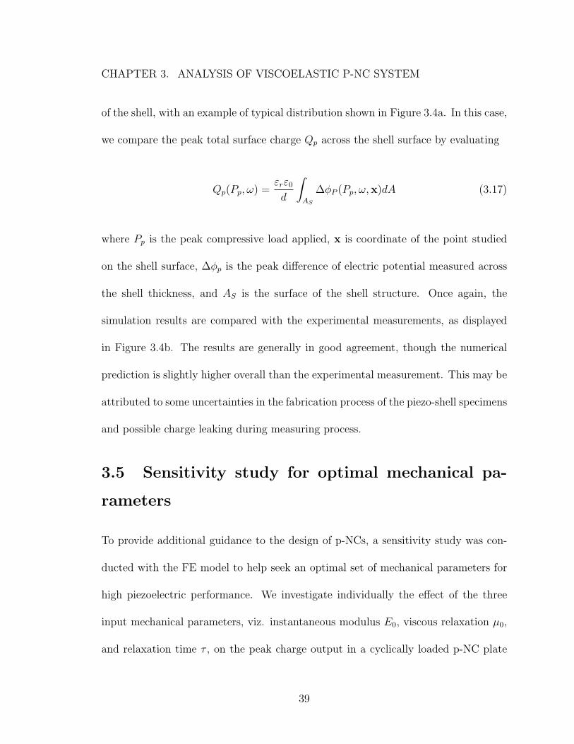
To further verify the robustness of the calibrated FE model, a set of dynamic load-

ing tests of flexible 3D piezo-shells was also simulated, with the configuration shown

in Figure 3.4a. It is worthwhile to note that, in this configuration, the piezoelectric

material is poled along the radial direction of the curved shell structure, and the plate

is grounded across its inner surface, i.e. φ(r = ri) = 0 with ri being the inner radius of

the half-cylinder shell structure. Since the piezoelectric coupling is performed in the

reference configuration, update of the piezoelectric constant tensor is not necessary

during the simulation of finite deformation process. Due to the deformation field in

the bent structure, the electric potential field is non-uniform along the outer surface

38


of the shell, with an example of typical distribution shown in Figure 3.4a. In this case,

we compare the peak total surface charge Qp across the shell surface by evaluating

Qp(Pp, ω) =εrε0d

∫

AS

∆φP (Pp, ω,x)dA (3.17)

where Pp is the peak compressive load applied, x is coordinate of the point studied

on the shell surface, ∆φp is the peak difference of electric potential measured across

the shell thickness, and AS is the surface of the shell structure. Once again, the

simulation results are compared with the experimental measurements, as displayed

in Figure 3.4b. The results are generally in good agreement, though the numerical

prediction is slightly higher overall than the experimental measurement. This may be

attributed to some uncertainties in the fabrication process of the piezo-shell specimens

and possible charge leaking during measuring process.

3.5 Sensitivity study for optimal mechanical pa-

rameters

To provide additional guidance to the design of p-NCs, a sensitivity study was con-

ducted with the FE model to help seek an optimal set of mechanical parameters for

high piezoelectric performance. We investigate individually the effect of the three

input mechanical parameters, viz. instantaneous modulus E0, viscous relaxation µ0,

and relaxation time τ , on the peak charge output in a cyclically loaded p-NC plate

39


polarized in the loading direction, i.e. the configuration shown in Figure 3.2a. For a

given set of (E0, µ0, τ), we may determine the storage modulus at an assigned load-

ing frequency according to Equation 3.13. Then, we utilize the available data of

experimentally measured pairs of storage and loss moduli in the manufactured p-NC

specimens to interpolate the corresponding loss modulus E′′

given a storage modulus

E′

. Experiments results, as discussed earlier, confirm that permittivity is not sig-

nificantly altered by the adjustment of the mechanical parameters in the polymeric

matrix. Maintaining a constant value of piezo-particle volume ratio in the compos-

ite while adjusting the parameters (E0, µ0, τ), the piezoelectric constant d33(E′

, E′′

)

can be calculated according to Equation 3.11. In the sensitivity study, the loading

condition is set to be uniaxial cyclic compression at 10Hz, with pattern described by

Equation 3.11 and maximum load set to 400 Pa.

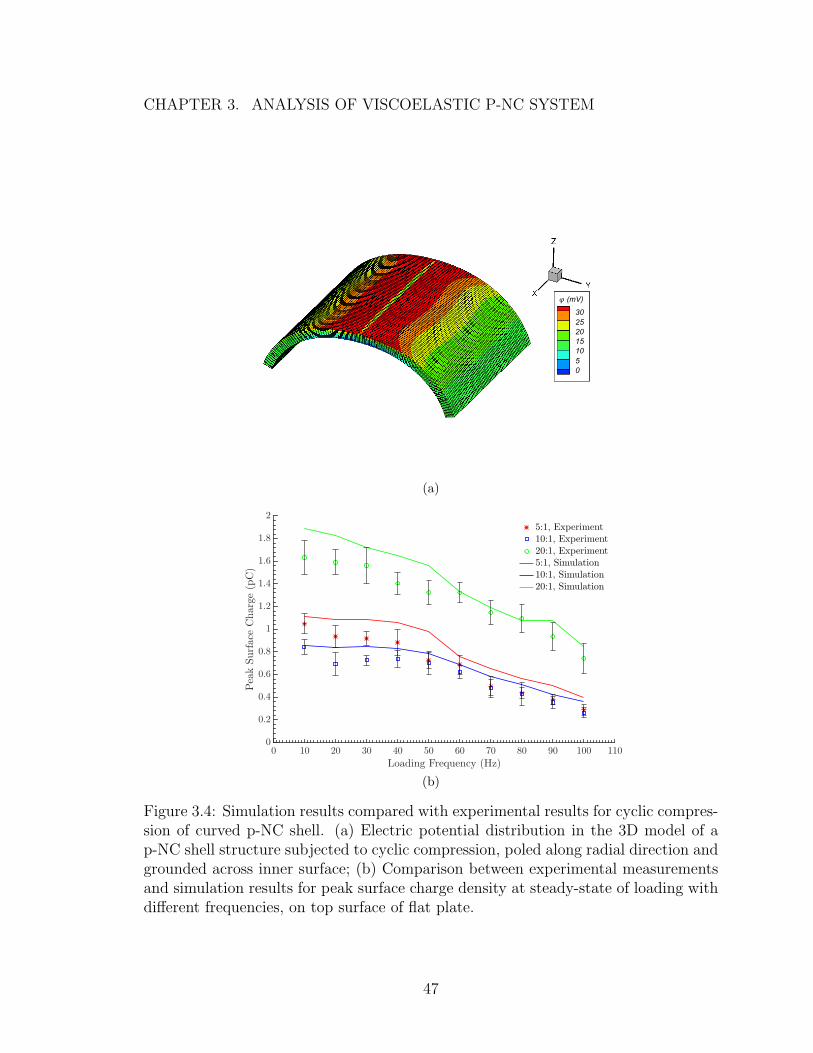
Figure 3.5 shows the change in time history of surface charge density when we ad-

just E0, µ0, and τ , respectively, while keeping the other mechanical input parameters

constant between the examined sets. As indicated in Figure 3.5a, when the overall

stiffness of the p-NC material is decreased, an increase in piezoelectric output is ob-

served, which is in agreement with the experimental observations discussed earlier.

In specific, a decrease of elastic modulus by 50% and 75% allowed for an increase of

steady-state piezoelectric output by 36% and 76%, respectively.

In the load-control setting examined here, this is due to the overall increase of

piezoelectric constant d33(E′

, E′′

) when E′

decreases significantly. To examine this

40


phenomenon, we may write Equation 3.11 in a rearranged form

d33 = εc

√

2Vpiezo

V εpiezo

√

E ′/2− πE ′′/4

E ′2 + E ′′2= εc

√

2Vpiezo

V εpiezoA(E

′

, E′′

) (3.18)

where the change of the parameter A(E′

, E′′

) following the adjustment of E′

and E′′

dictates the change of piezoelectric performance. For the experimentally measured

pairs of (E′

, E′′

), the corresponding values of A(E′

, E′′

) is shown in Figure 3.5b, with

A(E′

, E′′

) clearly displaying a decrease when E′

is greatly increased. This sheds light

on why higher piezoelectric output is observed in the softer p-NC specimens, and that

a lower overall modulus is desired in this class of material.

The effect of material relaxation on the piezoelectric output can be examined

according to the results shown in Figure 3.5c. When one-way cyclic loading is applied

to the viscoelastic material, as done in the present set of simulations, relaxation in

elastic modulus leads to residual stress when the material is fully unloaded at the end

of a loading cycle, which is converted to residual surface charge in the viscoelastic-

piezoelectric system studied. The buildup of residual charge after each loading cycle

leads to the gradual increase of peak surface charge, until the system finally reaches

an equilibrium state. It can be observed from Figure 3.5c that a higher µ0 allows for a

more significant amount of relaxation in the material, and therefore a greater increase

of peak surface charge after multiple cycles of one-way loading. This suggests that,

for applications where one-way dynamic loading is anticipated, increased amount of

41


viscous relaxation is beneficial for higher piezoelectric peak output.

Figure 3.5e shows the effect of relaxation time, τ , on the time history of surface

charge density. In this case, given an applied loading frequency of 10 Hz and constant

E0 and µ0 in the material model, a moderate relaxation time, τ = 0.1 s, produces

higher steady-state peak surface charge than measured in the models with much

shorter, τ = 0.01 s, or much longer relaxation time, τ = 1.0 s. This can be explained

by the fact that viscoelastic solids respond to loadings in an elastic manner, when

undergoing very fast or very slow processes [64–66]. When the loading cycle is very

long relative to the length of the relaxation time, the viscoelastic material behaves ef-

fectively as a softened elastic solid, and minimal residual stress is accumulated during

the loading-unloading process. When the loading cycle is very short relative to the

relaxation time, there is insufficient time for a considerable amount of viscous energy

dissipation to take place, and therefore the viscoelastic material behaves effectively

as a stiff elastic solid. We may thus conclude that, when the ratio of loading cycle

length to relaxation time is too low or too high, mechanical behavior of the material

converges towards elasticity, and, consequentially, we are unable to take advantage

of viscous relaxation to increase steady-state charge output. In order to maximize

piezoelectric output, the relaxation time of the material should be tailored to match

closely with the expected loading frequency. However, if it is more desirable for the

effect of viscous relaxation to be minimized, the relaxation time should be adjusted

to be much higher or much lower than the expected loading frequency.

42


3.6 Conclusion

Using the multiphysics finite element framework reviewed in Chapter 2, simulations

were performed to investigate the behavior of viscoelastic p-NC systems. Numerical

models were calibrated by incorporating experimentally measured mechanical prop-

erties and analytical prediction of piezoelectric constant into a multi-physics finite

element framework. Sensitivity studies were performed using numerical model to

investigate the relations between input parameters of the p-NC model and the piezo-

electric output to provide guidance for a desired set of mechanical properties in the

studied configuration.

It is found that, given cyclic compression loading with a constant value of peak

load, higher loading frequency corresponds to a lower level of peak output at steady-

state. Additionally, a decrease of elastic modulus allowed for an increase of steady-

state piezoelectric output in the p-NC material. The effect of viscous energy dis-

sipation can also be reduced by tailoring the material relaxation time to be much

shorter or longer than the length of applied loading cycle. Based on these findings,

the energy harvesting and the sensing performance of p-NCs can be further enhanced

by properly harnessing the viscoelasticity of piezocomposites.

43


0 20 40 60 80 100

Loading Frequency (Hz)

0

0.5

1

1.5

2

2.5

3

3.5

4

StorageModulus(P

a)

×106

5:110:120:1

(a)

0 20 40 60 80 100


0

2

4

6

8

10

LossModulus(P

a)

×105

5:110:120:1

(b)

Figure 3.1: Experimental measurement of dynamic moduli in the viscoelastic p-NCspecimens: (a) comparison of storage moduli at different loading frequencies; (b)comparison of loss moduli at different loading frequencies.

44


(a)

0 10 20 30 40 50 60 70 80 90 100 110


0

0.5

1

1.5

2

2.5

3

SurfaceCharge

Density

(C/m

2)

×10−8

5:1, Experiment10:1, Experiment20:1, Experiment5:1, Simulation10:1, Simulation20:1, Simulation

(b)

Figure 3.2: Simulation results compared with experimental results for cyclic com-pression of p-NC plate. (a) 3D model and mesh of the flat plate subjected to cycliccompressive loading; (b) Comparison between experimental measurements and simu-lation results for peak surface charge density at steady-state of loading with differentfrequencies, on top surface of flat plate.

45


100 101 102

|Tp| (kPa)

100

102

104PeakSurface

ChargeDen

sity

(C/m

2)

ν = 0.499, Compressionν = 0.499, Tensionν = 0.30, Compressionν = 0.30, Tension

(a)

0 0.5 1 1.5

Time (s)

-5

0

5

10

15

SurfaceCharge

Density

(C/m

2)

×10−8


(b)

0 0.5 1 1.5

Time (s)

-1

0

1

2

3

4

5

6

SurfaceCharge

Density

(C/m

2)

×10−6


(c)

0 0.5 1 1.5

Time (s)

0

2

4

6

8

SurfaceCharge

Density

(C/m

2)

×10−4


(d)

0 0.5 1 1.5

Time (s)

-6

-4

-2

0

2

4

6

8

SurfaceCharge

Density

(C/m

2) ×10−7

(e)

0 0.5 1 1.5

Time (s)

-5

0

5

10

15

SurfaceCharge

Density

(C/m

2) ×10−6

(f)

Figure 3.3: Simulation results for p-NC models under cyclic large deformation: (a)peak magnitude of surface charge density for compressible and nearly-incompressiblemodels of 20:1 p-NC under large cyclic deformation of 10 Hz; (b),(c),(d) comparisonof surface charge density time history under compressive and tensile cyclic loading ofpeak load magnitude 1 kPa, 10 kPa, 100 kPa; (e),(f) Detailed view of surface chargedensity time history under compressive cyclic loading of peak load magnitude 10 kPa,100 kPa;

46


(a)

0 10 20 30 40 50 60 70 80 90 100 110


0

0.2

0.4

0.6

0.8

1

1.2

1.4

1.6

1.8

2

PeakSurfaceCharge

(pC)

5:1, Experiment10:1, Experiment20:1, Experiment5:1, Simulation10:1, Simulation20:1, Simulation

(b)

Figure 3.4: Simulation results compared with experimental results for cyclic compres-sion of curved p-NC shell. (a) Electric potential distribution in the 3D model of ap-NC shell structure subjected to cyclic compression, poled along radial direction andgrounded across inner surface; (b) Comparison between experimental measurementsand simulation results for peak surface charge density at steady-state of loading withdifferent frequencies, on top surface of flat plate.

47


0.6 0.65 0.7 0.75 0.8 0.85 0.9 0.95 1

Time (s)

0

0.2

0.4

0.6

0.8

1

1.2

1.4

1.6

1.8

2

SurfaceCharge

Density

(C/m

2)

×10−8

G0 = 0.5 MPaG0 = 1.0 MPaG0 = 2.0 MPa

(a)

0 0.5 1 1.5 2 2.5 3

G′ (MPa)

3

4

5

6

7

8

9

A(1/√

Pa)

×10−4

20:1 p-NC10:1 p-NC5:1 p-NC

(b)

0 0.2 0.4 0.6 0.8 1

Time (s)

0

0.2

0.4

0.6

0.8

1

1.2

1.4

1.6

1.8

2

SurfaceCharge

Density

(C/m

2)

×10−8

µ0 = 0.1µ0 = 0.2µ0 = 0.4

(c)

0.6 0.7 0.8 0.9 1

Time (s)

1.1

1.2

1.3

1.4

1.5

1.6

SurfaceCharge

Density

(C/m

2) ×10−8

(d)

0 0.1 0.2 0.3 0.4 0.5 0.6 0.7 0.8 0.9 1

Time (s)

0

0.2

0.4

0.6

0.8

1

1.2

1.4

1.6

1.8

Surface

Charge

Density

(C/m

2)

×10−8

τ = 0.01 sτ = 0.1 sτ = 1 s

(e)

0.6 0.7 0.8 0.9 1

Time (s)

1.25

1.3

1.35

1.4

Surface

ChargeDensity

(C/m

2)

×10−8

(f)

Figure 3.5: Results of sensitivity studies: (a) Time history of surface charge density,for p-NC models with different instantaneous elastic modulus E0; (b) Dependence ofviscoelastic contribution factor A(E

′

) on storage modulus E′

, based on experimentmeasurements. (c) Time history of surface charge density, for p-NC models withdifferent viscous relaxation proportion µ0; (d) Detailed comparison of steady-statesurface charge density, for p-NC models with different viscous relaxation proportionµ0; (e) Time history of surface charge density, for p-NC models with different relax-ation time τ ; (f) Detailed comparison of steady-state surface charge density, for p-NCmodels with different relaxation time τ .

48

Chapter 4

Conclusions and Perspectives

Utilizing a multiphysics finite element model coupling transient electromagnetic

and dynamic mechanical fields in the time domain, computational analysis is per-

formed to analyze the piezoelectric behavior of viscoelastic p-NC structures under

dynamic loading conditions. The process served as validation for the model frame-

work to robustly predict the behavior of viscoelastic-piezoelectric systems subject to

dynamic finite deformation. Additionally, the problems of interest in the present

study are examples of coupled multiphysics problems that can be efficiently solved

with the introduced computational framework.

In the model framework, the coupling scheme maps Maxwell’s equations from spa-

tial to material coordinates in the reference configuration, allowing for the analysis of

finite deformation and its effect on the electromagnetic field variables. The framework

is able to predict the evolution of electrical and magnetic fields in a vibrating media

undergoing finite deformation, with capabilities unavailable in current commercial

codes for multiphysics analysis.

Input parameters of the computational model is calibrated according to exper-

49

CHAPTER 4. CONCLUSIONS AND PERSPECTIVES

imental measurements to reproduce the piezoelectric behavior of viscoelastic p-NC

structures under cyclic loading of various frequencies. Additional simulations are

performed to investigate the response of the p-NC model under dynamic large defor-

mation, further validating the capability of the finite element model to predict the

piezoelectric performance of the p-NC systems.

A sensitivity study is conducted to provide additional guidance to the design of

p-NCs. By adjusting the input mechanical parameters in the material model, viz.

instantaneous modulus E0, viscous relaxation µ0, and relaxation time τ , an optimal

set of mechanical parameters is determined for high piezoelectric performance. It is

found that, under a load-controlled cyclic loading condition, piezoelectric output is

higher in p-NC with lower instantaneous modulus. The increase of viscous relaxation,

i.e. higher µ0, corresponds to a large amount of residual stress at the end of a single-

direction loading cycle. In the case of cyclic compression or cyclic tension loading,

p-NC with high µ0 produced higher peak charge output at steady-state. The effect

of viscous relaxation is strongest when the relaxation time τ of the viscous material

model has a magnitude comparable to the cycle length of the applied loading. When

the loading cycle is much longer or shorter than the relaxation time, the p-NC behaves

similar to an elastic material. According to the specific application of the material, the

mechanical parameters can be tailored to produce optimal piezoelectric performance

under dynamic loading conditions. The calibrated material model can be also further

applied to guide the design of p-NC systems with complex structures, under different

50

CHAPTER 4. CONCLUSIONS AND PERSPECTIVES

dynamic loading conditions which cannot be easily tested with experiments. In future

works, the computational model may be further improved by explicitly modeling the

nanostructure of the p-NC material to accurately capture the interactions between

the polymeric matrix, piezoparticles, and nanofillers.

51

Bibliography

[1] Xiaoliang Zhao, Huidong Gao, Guangfan Zhang, Bulent Ayhan, Fei Yan, Chiman

Kwan, and Joseph L Rose. Active health monitoring of an aircraft wing with

embedded piezoelectric sensor/actuator network: I. defect detection, localization

and growth monitoring. Smart materials and structures, 16(4):1208, 2007.

[2] Jinzhu Zhou, Jin Huang, Qingqang He, Baofu Tang, and Liwei Song. Develop-

ment and coupling analysis of active skin antenna. Smart Materials and Struc-

tures, 26(2):025011, 2016.

[3] Thomas Bailey and JE Ubbard. Distributed piezoelectric-polymer active vibra-

tion control of a cantilever beam. Journal of Guidance, Control, and Dynamics,

8(5):605–611, 1985.

[4] Kt Chandrashekhara and AN Agarwal. Active vibration control of laminated

composite plates using piezoelectric devices: a finite element approach. Journal

of Intelligent Material Systems and Structures, 4(4):496–508, 1993.

[5] Vladimir M Shalaev. Optical negative-index metamaterials. Nature photonics,

1(1):41–48, 2007.

52

BIBLIOGRAPHY

[6] Wenshan Cai and Vladimir Shalaev. Optical metamaterials: fundamentals and

applications. Springer Science & Business Media, 2009.

[7] Yugang Sun, Won Mook Choi, Hanqing Jiang, Yonggang Y Huang, and John A

Rogers. Controlled buckling of semiconductor nanoribbons for stretchable elec-

tronics. Nature nanotechnology, 1(3):201–207, 2006.

[8] Alfred J Baca, Jong-Hyun Ahn, Yugang Sun, Matthew A Meitl, Etienne Menard,

Hoon-Sik Kim, Won Mook Choi, Dae-Hyeong Kim, Young Huang, and John A

Rogers. Semiconductor wires and ribbons for high-performance flexible electron-

ics. Angewandte Chemie International Edition, 47(30):5524–5542, 2008.

[9] John A Rogers, Takao Someya, and Yonggang Huang. Materials and mechanics

for stretchable electronics. Science, 327(5973):1603–1607, 2010.

[10] Nanshu Lu and Shixuan Yang. Mechanics for stretchable sensors. Current Opin-

ion in Solid State and Materials Science, 19(3):149–159, 2015.

[11] Tayfun Ozdemir and John L Volakis. Triangular prisms for edge-based vector

finite element analysis of conformal antennas. IEEE Transactions on Antennas

and Propagation, 45(5):788–797, 1997.

[12] Waldemar Rachowicz and L Demkowicz. An hp-adaptive finite element method

for electromagneticspart ii: A 3d implementation. International journal for nu-

merical methods in engineering, 53(1):147–180, 2002.

53

BIBLIOGRAPHY

[13] Witold Cecot, Waldemar Rachowicz, and L Demkowicz. An hp-adaptive finite

element method for electromagnetics. part 3: A three-dimensional infinite ele-

ment for maxwell’s equations. International journal for numerical methods in

engineering, 57(7):899–921, 2003.

[14] Leszek Demkowicz, Jason Kurtz, and Frederick Qiu. hp-adaptive finite elements

for coupled multiphysics wave propagation problems. Computer Methods in Me-

chanics, pages 19–42, 2010.

[15] Jesse D Thomas and Nicolas Triantafyllidis. On electromagnetic forming pro-

cesses in finitely strained solids: Theory and examples. Journal of the Mechanics

and Physics of Solids, 57(8):1391–1416, 2009.

[16] Jesse D Thomas, Nicolas Triantafyllidis, A Vivek, Glenn S Daehn, and John R

Bradley. Comparison of fully coupled modeling and experiments for electro-

magnetic forming processes in finitely strained solids. International Journal of

Fracture, 163(1):67–83, 2010.

[17] AS Semenov, H Kessler, A Liskowsky, and H Balke. On a vector potential for-

mulation for 3d electromechanical finite element analysis. International Journal

for Numerical Methods in Biomedical Engineering, 22(5):357–375, 2006.

[18] Alejandro Mota and Jonathan A Zimmerman. A variational, finite-deformation

constitutive model for piezoelectric materials. International journal for numerical

methods in engineering, 85(6):752–767, 2011.

54

BIBLIOGRAPHY

[19] Shu Guo and Somnath Ghosh. A finite element model for coupled 3d transient

electromagnetic and structural dynamics problems. Computational Mechanics,

54(2):407–424, 2014.

[20] Reza Yaghmaie, Shu Guo, and Somnath Ghosh. Wavelet transformation in-

duced multi-time scaling (watmus) model for coupled transient electro-magnetic

and structural dynamics finite element analysis. Computer Methods in Applied

Mechanics and Engineering, 303:341–373, 2016.

[21] Shu Guo. A Coupled Multi-physics Analysis Model for Integrating Transient

Electro-Magnetics and Structural Dynamic Fields with Damage. PhD thesis,

Johns Hopkins University, 2017.

[22] M Lax and DF Nelson. Maxwell equations in material form. Physical Review B,

13(4):1777, 1976.

[23] Carmine Trimarco. Material electromagnetic fields and material forces. Archive

of Applied Mechanics, 77(2):177–184, 2007.

[24] Carmine Trimarco. On the dynamics of electromagnetic bodies. International

Journal of Advances in Engineering Sciences and Applied Mathematics, 1(4):157–

162, 2009.

[25] Juan Carlos Simo. On a fully three-dimensional finite-strain viscoelastic damage

55

BIBLIOGRAPHY

model: formulation and computational aspects. Computer methods in applied

mechanics and engineering, 60(2):153–173, 1987.

[26] Olgierd Cecil Zienkiewicz and Robert Leroy Taylor. The finite element method:

solid mechanics, volume 2. Butterworth-heinemann, 2000.

[27] Donald Frederick Nelson. Electric, optic, and acoustic interactions in dielectrics.

John Wiley & Sons, 1979.

[28] L Vu-Quoc, V Srinivas, and Y Zhai. A generalized unit system for concise

electromagnetic formulation and accurate numerical solutions. Journal of Com-

putational Physics, 181(2):407–429, 2002.

[29] Jian-Ming Jin. The finite element method in electromagnetics. John Wiley &

Sons, 2015.

[30] W Nowacki. Foundations of linear piezoelectricity. Electromagnetic interactions

in elastic solids, 257:105–157, 1979.

[31] A Meitzler, HF Tiersten, AW Warner, D Berlincourt, GA Couqin, and

FS Welsh III. Ieee standard on piezoelectricity, 1988.

[32] C Miehe, D Rosato, and B Kiefer. Variational principles in dissipative electro-

magneto-mechanics: A framework for the macro-modeling of functional materi-

als. International Journal for Numerical Methods in Engineering, 86(10):1225–

1276, 2011.

56

BIBLIOGRAPHY

[33] Gerhard A Holzapfel. Nonlinear solid mechanics. 2000.

[34] Joao Pedro A Bastos and Nelson Sadowski. Electromagnetic modeling by finite

element methods. CRC press, 2003.

[35] Klaus-Jurgen Bathe and Edward L Wilson. Numerical methods in finite element

analysis, volume 197. Prentice-Hall Englewood Cliffs, NJ, 1976.

[36] K Subbaraj and MA Dokainish. A survey of direct time-integration methods in

computational structural dynamicsii. implicit methods. Computers & Structures,

32(6):1387–1401, 1989.

[37] MA Dokainish and K Subbaraj. A survey of direct time-integration methods in

computational structural dynamicsi. explicit methods. Computers & Structures,

32(6):1371–1386, 1989.

[38] George Karypis, Kirk Schloegel, and Vipin Kumar. Parmetis: Parallel graph

partitioning and sparse matrix ordering library. Version 1.0, Dept. of Computer

Science, University of Minnesota, 1997.

[39] Satish Balay, J Brown, Kris Buschelman, Victor Eijkhout, W Gropp, D Kaushik,

M Knepley, L Curfman McInnes, B Smith, and Hong Zhang. Petsc users manual

revision 3.5. Argonne National Laboratory (ANL), 2014.

[40] Zhong Lin Wang and Jinhui Song. Piezoelectric nanogenerators based on zinc

oxide nanowire arrays. Science, 312(5771):242–246, 2006.

57

BIBLIOGRAPHY

[41] Luana Persano, Canan Dagdeviren, Yewang Su, Yihui Zhang, Salvatore Girardo,

Dario Pisignano, Yonggang Huang, and John A Rogers. High performance piezo-

electric devices based on aligned arrays of nanofibers of poly (vinylidenefluoride-

co-trifluoroethylene). Nature communications, 4:1633, 2013.

[42] Geon-Tae Hwang, Hyewon Park, Jeong-Ho Lee, SeKwon Oh, Kwi-Il Park,

Myunghwan Byun, Hyelim Park, Gun Ahn, Chang Kyu Jeong, Kwangsoo No,

et al. Self-powered cardiac pacemaker enabled by flexible single crystalline pmn-

pt piezoelectric energy harvester. Advanced materials, 26(28):4880–4887, 2014.

[43] Po-Kang Yang, Long Lin, Fang Yi, Xiuhan Li, Ken C Pradel, Yunlong Zi, Chih-

I Wu, Hau He Jr, Yue Zhang, and Zhong Lin Wang. A flexible, stretchable

and shape-adaptive approach for versatile energy conversion and self-powered

biomedical monitoring. Advanced Materials, 27(25):3817–3824, 2015.

[44] Xu Xiao, Longyan Yuan, Junwen Zhong, Tianpeng Ding, Yu Liu, Zhixiang Cai,

Yaoguang Rong, Hongwei Han, Jun Zhou, and Zhong Lin Wang. High-strain

sensors based on zno nanowire/polystyrene hybridized flexible films. Advanced

materials, 23(45):5440–5444, 2011.

[45] Santiago Orrego, Kourosh Shoele, Andre Ruas, Kyle Doran, Brett Caggiano,

Rajat Mittal, and Sung Hoon Kang. Harvesting ambient wind energy with an

inverted piezoelectric flag. Applied Energy, 194:212–222, 2017.

[46] Sangmin Lee, Sung-Hwan Bae, Long Lin, Ya Yang, Chan Park, Sang-Woo Kim,

58

BIBLIOGRAPHY

Seung Nam Cha, Hyunjin Kim, Young Jun Park, and Zhong Lin Wang. Super-

flexible nanogenerator for energy harvesting from gentle wind and as an active

deformation sensor. Advanced Functional Materials, 23(19):2445–2449, 2013.

[47] Rusen Yang, Yong Qin, Cheng Li, Guang Zhu, and Zhong Lin Wang. Converting

biomechanical energy into electricity by a muscle-movement-driven nanogenera-

tor. Nano Letters, 9(3):1201–1205, 2009.

[48] Guang Zhu, Rusen Yang, Sihong Wang, and Zhong Lin Wang. Flexible

high-output nanogenerator based on lateral zno nanowire array. Nano letters,

10(8):3151–3155, 2010.

[49] Yi Qi, Noah T Jafferis, Kenneth Lyons Jr, Christine M Lee, Habib Ahmad,

and Michael C McAlpine. Piezoelectric ribbons printed onto rubber for flexible

energy conversion. Nano letters, 10(2):524–528, 2010.

[50] Yi Qi, Jihoon Kim, Thanh D Nguyen, Bozhena Lisko, Prashant K Purohit,

and Michael C McAlpine. Enhanced piezoelectricity and stretchability in energy

harvesting devices fabricated from buckled pzt ribbons. Nano letters, 11(3):1331–

1336, 2011.

[51] Kwi-Il Park, Sheng Xu, Ying Liu, Geon-Tae Hwang, Suk-Joong L Kang,

Zhong Lin Wang, and Keon Jae Lee. Piezoelectric batio3 thin film nanogen-

erator on plastic substrates. Nano letters, 10(12):4939–4943, 2010.

59

BIBLIOGRAPHY

[52] Chieh Chang, Van H Tran, Junbo Wang, Yiin-Kuen Fuh, and Liwei Lin. Direct-

write piezoelectric polymeric nanogenerator with high energy conversion effi-

ciency. Nano letters, 10(2):726–731, 2010.

[53] Minbaek Lee, Chih-Yen Chen, Sihong Wang, Seung Nam Cha, Yong Jun Park,

Jong Min Kim, Li-Jen Chou, and Zhong Lin Wang. A hybrid piezoelectric

structure for wearable nanogenerators. Advanced Materials, 24(13):1759–1764,

2012.

[54] Kwi-Il Park, Minbaek Lee, Ying Liu, San Moon, Geon-Tae Hwang, Guang Zhu,

Ji Eun Kim, Sang Ouk Kim, Do Kyung Kim, Zhong Lin Wang, et al. Flexible

nanocomposite generator made of batio3 nanoparticles and graphitic carbons.

Advanced Materials, 24(22):2999–3004, 2012.

[55] Ke Yang, Xingyi Huang, Yanhui Huang, Liyuan Xie, and Pingkai Jiang. Fluoro-

polymer@ batio3 hybrid nanoparticles prepared via raft polymerization: toward

ferroelectric polymer nanocomposites with high dielectric constant and low di-

electric loss for energy storage application. Chemistry of Materials, 25(11):2327–

2338, 2013.

[56] Sung-Ho Shin, Young-Hwan Kim, Min Hyung Lee, Joo-Yun Jung, and Junghyo

Nah. Hemispherically aggregated batio3 nanoparticle composite thin film for

high-performance flexible piezoelectric nanogenerator. ACS nano, 8(3):2766–

2773, 2014.

60

BIBLIOGRAPHY

[57] Indu Babu and Gijsbertus de With. Highly flexible piezoelectric 0–3 pzt–pdms

composites with high filler content. Composites Science and Technology, 91:91–

97, 2014.

[58] HM Ning, N Hu, T Kamata, JH Qiu, X Han, LM Zhou, Christiana Chang,

Y Liu, LK Wu, HL Ji, et al. Improved piezoelectric properties of poly (vinyli-

dene fluoride) nanocomposites containing multi-walled carbon nanotubes. Smart

materials and structures, 22(6):065011, 2013.

[59] Vahabodin Goodarzi and Mohammad Reza Saeb. Modeling and interpreting

particle shape dependence of electric displacement distribution in the piezoelec-

tric polymer composites. Journal of Intelligent Material Systems and Structures,

27(17):2395–2407, 2016.

[60] Shogo Mamada, Naoyuki Yaguchi, Masanori Hansaka, Masafumi Yamato, and

Hirohisa Yoshida. Matrix influence on the piezoelectric properties of piezoelectric

ceramic/polymer composite exhibiting particle alignment. Journal of Applied

Polymer Science, 132(15), 2015.

[61] Nicholas W Tschoegl. The phenomenological theory of linear viscoelastic behav-

ior: an introduction. Springer Science & Business Media, 2012.

[62] Norman Gerard McCrum, CP Buckley, and Clive B Bucknall. Principles of

polymer engineering. Oxford University Press, USA, 1997.

61

BIBLIOGRAPHY

[63] Richard Christensen. Theory of viscoelasticity: an introduction. Elsevier, 2012.

[64] Roderic S Lakes. Viscoelastic materials. Cambridge University Press, 2009.

[65] Clarence Zener. Elasticity and anelasticity of metals. University of Chicago press,

1948.

[66] John D Ferry. Viscoelastic properties of polymers. John Wiley & Sons, 1980.

62

Vita

Zhiren Zhu was born in Sendai, and spent childhood years living in Japan, the

United States, Norway, and China. Zhiren received the B.S. degree in Civil Engineer-

ing from the University of Massachusetts Amherst in 2013 and the M.S. degree in

Structural Engineering and Mechanics from the University of Minnesota, Minneapo-

lis in 2015.

Starting in August 2017, Zhiren will work as a junior foundations engineer at

Berkel and Company Contractors in Silver Spring, MD.

63

Computational Analysis of Piezoelectric Systems Using A ...

Documents

Transcript of Computational Analysis of Piezoelectric Systems Using A ...