Texas A&M University Mechanical Engineering Department

Turbomachinery Laboratory Tribology Group

Computational Analysis of Gas Foil Bearings

Integrating 1D and 2D Finite Element Models

for Top Foil

Research Progress Report to the TAMU Turbomachinery Research Consortium

TRC-B&C-1-06

by

Luis San Andrés Mast-Childs Professor

Principal Investigator

Tae Ho Kim Research Assistant

June 2006

This material is based upon work supported by the National Science Foundation under Grant No. 0322925

Gas Foil Bearings for Oil-Free Rotating Machinery – Analysis Anchored to

Experiments NSF Funded Project, TEES # 32525/53900/ME

ii

EXECUTIVE SUMMARY

Gas foil bearings (GFBs) are finding widespread usage in oil-free turbo expanders, APUs and

micro gas turbines for distributed power due to their low drag friction and ability to tolerate high

level vibrations, including transient rubs and severe misalignment, static and dynamic. The static

load capacity and dynamic forced performance of GFBs depends largely on the material

properties of the support elastic structure, i.e. a smooth foil on top of bump strip layers.

Conventional models include only the bumps as an equivalent stiffness uniformly distributed

around the bearing circumference. More complex models couple directly the elastic deformations

of the top foil to the bump underlying structure as well as to the hydrodynamics of the gas film.

This report details two FE models for the top foil supported on bump strips, one considers a 2D

shell anisotropic structure and the other a 1D beam-like structure. The decomposition of the

stiffness matrix representing the top foil and bump strips into upper and lower triangular parts is

performed off-line and prior to computations coupling it to the gas film analysis governed by

Reynolds equation. The procedure greatly enhances the computational efficiency of the

numerical scheme.

Predictions of load capacity, attitude angle, and minimum film thickness versus journal speed

are obtained for a GFB tested decades ago. 2D FE model predictions overestimate the minimum

film thickness at the bearing centerline, but underestimate it at the bearing edges. Predictions

from the 1D FE model compare best to the limited tests data; reproducing closely the

experimental circumferential profile of minimum film thickness. The 1D top foil model is to be

preferred due to its low computational cost. Predicted stiffness and damping coefficients versus

excitation frequency show that the two FE top foil structural models result in slightly lower

direct stiffness and damping coefficients than those from the simple elastic foundation model.

A three lobe GFB with mechanical preloads, introduced by inserting shims underneath the

bump strips, is analyzed using the 1D FE structural model. Predictions show the mechanical

preload enhances the load capacity of the gas foil bearing for operation at low loads and low

shaft speeds. Energy dissipation, a measure of the bearing ability to ameliorate vibrations, is not

affected by the preload induced. The mechanical preload has no effect on the static and dynamic

forced performance of GFBs supporting large static loads.

iii

TABLE OF CONTENTS EXECUTIVE SUMMARY ii

LIST OF TABLES iv

LIST OF FIGURES iv

NOMENCLATURE iv I. INTRODUCTION 1

II. LITERATURE REVIEW 3

III. DESCRIPTION OF GAS FOIL BEARINGS 6

MODELING OF FOIL SUPPORT STRUCTURE 7

IV.1 CONVENTIONAL SIMPLE ELASTIC FOUNDATION MODEL 7

IV.2 ONE DIMENSIONAL ELASTIC MODEL FOR TOP FOIL 8IV.

IV.3 TWO DIMENSIONAL MODEL FOR TOP FOIL 10

COMPARISONS OF PREDICTIONS TO PUBLISHED TEST DATA 16

V.1 CONFIGURATION OF TEST GFB 16

V.2 MINIMUM FIILM THICKNESS AND JOURNAL ATTITUDE

ANGLE 17

V.

V.3 PREDICTED STIFFNESS AND DAMPING FORCE COEFFICEINTS 26

VI. COMPUTATIONAL TIME 32

VII. EFFECT OF MECHANICAL PRELOAD ON THE FORCED PERFORMANCE

OF A GFB 33

VIII. CLOSURE 46

IX. REFERENCES 48

APPENDIX A 1D FINITE ELEMENT FORMULATION FOR TOP FOIL 51

APPENDIX B 2D FINTIE ELEMENT FORMULATION FOR TOP FOIL 53

iv

LIST OF TABLES

1 Design details of foil bearing, reference [19] 16

2 Geometry of foil bearing with mechanical preload (shims) 34

LIST OF FIGURES

1 Typical Gas Foil Bearings (GFBs) for oil-free turbomachinery 1

2 Schematic view of first generation bump type foil bearing 6

3 Configuration of top foil supported on a bump strip and its 1D structural model. Generalized displacements: 1

eu =w1, 2eu =φ1, 3

eu =w2, and 4eu =φ2

9

4 Schematic representations of deformations in actual and idealized top foil and bump strips

10

5 Configuration of top foil supported on a bump strip and its 2D structural model 11

6 Resultant membrane forces and bending moments per unit shell element length for a distributed load in the domain of a shell finite element

12

7 Four-node, shell finite element supported on an axially distributed linear spring 14

8 Configuration of top foil and bump foil strips 17

9 Minimum film thickness versus static load. Predictions from three foil structural models and test data [19]

19

10 Axially averaged minimum film thickness versus static load. Predictions from 2D top foil model and test data [19]

20

11 Journal attitude angle versus static load. Predictions from three foil structural models and test data [19]

22

12 Journal eccentricity versus static load at 45 krpm, Predictions from three foil structural models for GFB in [19]

22

13 Predicted (a) dimensionless pressure field and (b) film thickness field from 2D top foil structural model. Static load: 200 N, rotor speed: 45 krpm. Bearing configuration given in [19]

24

14 Film thickness versus angular location at bearing mid-plane. Prediction from 1D top foil model and test data [19]. Static load: 134.1 N. Rotor speed: 30 krpm

25

15 Predicted GFB stiffness coefficients versus excitation frequency for three structural models. Rotor speed: 45 krpm, Static load: 150 N. Structural loss factor γ = 0.0.

28

16 Predicted GFB damping coefficients versus excitation frequency for three structural models. Rotor speed: 45 krpm, Static load: 150 N. Structural loss factors, γ = 0.0 and 0.4

31

17 Schematic views of gas foil bearing with (a) shims and (b) with machined preloads

33

18 Dimensionless mid-plane pressure, structural deflection, and film thickness versus angular location for GFB with and without mechanical preload. Rotor

35

v

speed: 45 krpm 19 Journal eccentricity versus static load for GFB with and without mechanical

preload. Rotor speed: 45,000 rpm 36

20 Journal attitude angle versus static load for for GFB with and without mechanical preload. Rotor speed: 45,000 rpm

37

21 Minimum film thickness versus static load for GFB with and without mechanical preload. Rotor speed: 45,000 rpm

37

22 Drag power loss versus static load for GFB with and without mechanical preload. Rotor speed: 45,000 rpm

38

23a Synchronous stiffness coefficients versus static load for GFB with and without preload. Rotor speed: 45,000 rpm, loss factor, γ=0.2

40

23b Synchronous damping coefficients versus static load for GFB with and without preload. Rotor speed: 45,000 rpm, loss factor, γ=0.2

41

24a Stiffness coefficients versus excitation frequency for GFB with and without mechanical preload. Static load: 5N, rotor speed: 45 krpm, loss factor, γ=0.2

42

24b Damping coefficients versus excitation frequency for GFB with and without mechanical preload. Static load: 5N, rotor speed: 45 krpm, loss factor, γ=0.2

43

25 Energy dissipated by a GFB with and without mechanical preload for increasing static loads. Rotor speed: 45 krpm, loss factor, γ=0.2

45

vi

NOMENCLATURE Cαβ Damping coefficients; , ,X Yα β = [N·s/m] c Nominal radial clearance [m]

Jc Measured journal radial travel [m] mc Assembly radial clearance [m]

D Top foil (bearing) diameter, 2D R= × [m] E Top foil elastic modulus [Pa] or [N/ m2] eX, eY Journal eccentricity component [m], 2 2

X Ye e e= + eF , GF FE element nodal force vector and global nodal force vector 1f Normal load vector for a four-node finite shell element.

h Gas film thickness [m] th Shell thickness [m] bh Bump height [m]

I Moment of inertia [m4] i Imaginary unit, 1− j Node number along circumferential direction

eK , GK FE top foil element stiffness matrix and global nodal stiffness matrix sK FE bump element stiffness matrix fK Structural stiffness per unit area [N/m3]

fK ′ Complex structural stiffness per unit area, ( )1f fK K iγ′ = + [N/m3]

lK Structural stiffness per unit bump element [N/m] Kαβ Stiffness coefficients; , ,X Yα β = [N/m] k Node number along the axial direction

ijk Stiffness matrices for a four-node finite element plate stiffness matrix tk Shear correction coefficient (=5/6) in a shear deformable plate model [-]

L Bearing axial width [m] xl Pad circumferential length, ( )t lR Θ −Θ [m] 0l Half bump length [m] exl FE thin foil length in the circumferential direction [m] eyl FE thin foil length in the axial direction [m]

MNM Bending moment per unit element length in a thin shell [N] 1,2m bending moment vectors for a four-node finite shell element MNN Membrane or in-plane force per unit element length in a thin shell [N/m] bN Number of bumps [-]

p Hydrodynamic pressure in gas film [Pa] pa Ambient pressure [Pa] pA Average pressure along axial direction [Pa]

mQ Shear force per unit element length in a thin shell [N/m]

1,2eQ Shear forces at the boundary of a FE element

3,4eQ Bending moments at the boundary of a FE element

vii

q Transversely distributed load [N/m2]. rP Preload on bearing [m] R Top foil (bearing) radius [m]

faS , fcS Stiffening factors for elastic modulus in the axial and circumferential directions [-] 0s Bump pitch [m]

t Time [s] bt Bump foil thickness [m] tt Top (thin) foil thickness [m]

eU , GU FE nodal displacement vector and global nodal displacement vector u Shell circumferential displacement (x direction)

eu FE nodal displacement w top foil transverse deflection [m]

,X Y Coordinate system for the inertial axes [m] ,x z Coordinate system on plane of bearing [m] xφ , yφ Shell rotation angles about the y and x axes Φ Journal attitude angle, tan-1(ex/ey) [rad] γ Structural damping loss factor [-] μ Gas viscosity [Pa-s] ν Shell axial displacement (y direction)

1,2ν Weight function for FE formulae pν Poisson’s ratio [-] eψ Hermite cubic interpolation function

Θ Top foil angular coordinate [rad] Θp Preload offset position [rad] Ω Rotor angular velocity [rad]

thresholdΩ Threshold speed of instability [Hz] ω Whirl frequency [rad]

thresholdω Whirl frequency of unstable motions[Hz] nω Natural frequency of system [Hz]

WFR thresholdω / thresholdΩ .Whirl frequency ratio [-] Subscripts

,α β = ,X Y Directions of perturbation for first order pressure fields ,M N = ,x y Directions of shell membrane and moment force

Superscripts i,j =1-3 Row and column numbers for a four-node finite element plate stiffness matrix

1

I. INTRODUCTION

Implementing gas foil bearings (GFBs) in micro turbomachinery reduces system

complexity and maintenance costs, and increases efficiency and operating life [1, 2].

Since the 1960s, tension tape GFBs and multiple leaf GFBs with and without backing

springs, as well as corrugated bump GFBs, have been implemented as low friction

supports in oil-free (small size) rotating machinery. In comparison to rolling element

bearings and for operation at high surface speeds, both leaf GFBs and bump GFBs have

demonstrated superior reliability in Air Cycle Machines (ACMs) of aircraft

environmental control systems [3-6], for example. Figure 1 shows the configurations of

two GFBs. In multiple overleaf GFBs, the compliance to bending from staggered

structural foils and the dry-friction at the contact lines define their operational

characteristics [5]. In corrugated bump GFBs, bump-strip layers supporting a top foil

render a tunable bearing stiffness with nonlinear elastic deformation characteristics. In

this type of bearing, dry-friction effects arising between the bumps and top foil and the

bumps and the bearing inner surface provide the energy dissipation or damping

characteristics [6].

(a) Multiple leaf GFB (b) Corrugated bump GFB

Figure 1. Typical Gas Foil Bearings for oil-free turbomachinery

The published literature notes that multiple leaf GFBs are not the best of supports in

high performance turbomachinery, primarily because of their inherently low load

capacity [6]. A corrugated bump type GFB fulfills most of the requirements of highly

Thin foilStructural bump

Rotor spinning

Housing

Leaf foil

2

efficient oil-free turbomachinery, with demonstrated ultimate load capacity up to 680 kPa

(100 psi) [7, 8].

The forced performance of a GFB depends upon the material properties and

geometrical configuration of its support structure (the top foil and bump strip layers), as

well as the hydrodynamic film pressure generated within the bearing clearance. In

particular, the underlying support structure dominates the static and dynamic

performance of high speed, heavily loaded GFBs [9]. For example, due to the elastic

deflection of the bump strip layers, GFBs show relatively small changes in film thickness

as compared to those in journal eccentricity. The GFB overall stiffness depends mainly

on the softer support structure, rather than on that of the gas film, which “hardens” as the

shaft speed and applied load increase. Material hysteresis and dry-friction dissipation

mechanisms between the bumps and top foil, as well as between the bumps and the

bearing inner surface, appear to enhance the bearing damping [10].

The envisioned application of GFBs into midsize gas turbine engines demands

accurate performance predictions anchored to reliable test data. Modeling of GFBs is

difficult due to the mechanical complexity of the bump-foil structure, further aggravated

by the lack of simple, though physically realistic, energy dissipation models at the contact

surfaces where dry-friction is prevalent.

In this report, the top foil, modeled as a structural shell using Finite Elements (FE), is

integrated with the bump strip layers and in conjunction with the hydrodynamic gas film

to predict the static and dynamic load performance of GFBs. Model predictions for two

types of top foil structures, one and two dimensional, are compared to limited test results

available in the literature. The effects of a mechanical preload on the GFB forced

performance and stability characteristics are also studied. Shims installed under a bump

strip layers at selected circumferential locations provide the preloads, thus modifying the

nominal film thickness of the gas foil bearing. The objective is to determine

enhancements in load capacity and rotordynamic instability for operation with small

static loads and at high rotor speeds.

3

II. LITERATURE REVIEW

In 1953 Blok and van Rossum [11] introduce the concept of Foil Bearings (FBs). The

authors point out that bearing film thickness, larger than that of rigid gas bearings, can

improve operational reliability and provide a solution for problems related to the thermal

expansion of both a journal and its bearing. Field experience has proved, since the late

1960’s, that Gas Foil Bearings (GFBs) are far more reliable than ball bearings that were

previously used in Air Cycle Machines (ACMs) installed in aircrafts. Therefore, GFBs

have since been used in almost every new ACM installed in both civil and military

aircraft [1]. This literature review discusses previous work related to the analysis of

corrugated bump type GFBs.

Implementation of GFBs into high performance applications demands accuracy in

modeling capabilities. Engineered GFBs must have a dimensionless load capacity larger

than unity, i.e. specific pressure (W/LD) > Pa [2].

Heshmat et al. [9,12] first present analyses of bump type GFBs and detail the bearings

static load performance. The predictive model couples the gas film hydrodynamic

pressure generation to a local deflection (wd) of the support bumps. In this simple of all

models, the top foil is altogether neglected and the elastic displacement wd = α (p-pa) is

proportional to the local pressure (p-pa) and a structural compliance (α) coefficient which

depends on the bump material, thickness and geometric configuration. This model,

ubiquitous in the literature of GFBs, is hereby known as the simple elastic foundation

model.

Peng and Carpino [13,14] present finite difference formulations to calculate the

linearized stiffness and damping force coefficients of GFBs. The model includes both

fluid (gas) film and structural bump layers used to simultaneously solve the Reynolds

equations, and a simple equation to calculate iteratively gas film thickness for compliant

GFBs. In the model of the underlying foil structure, a perfectly extensible foil is placed

on top of the corrugated bumps. The model considers two neighboring bumps are not

connected, i.e. no relative motion between them is assumed to occur.

Carpino et al. [15-17] have advanced the most complete computational models to date,

including detailed descriptions of membrane and bending effects of the top foil, and

accounting for the sub-foil structure elastic deformation. In [15,16], the authors build FE

4

models for the gas film and the foil structure, couple both models through the pressure

field and get solutions using an iterative numerical scheme.

The bending and membrane rigidity terms of the FE model for the foil structure are

not coupled so that the former and the latter render both the displacements for the

bending plate and elastic plane (or membrane) models, respectively. On the other hand,

[17] introduces a fully coupled finite element formulation for foil bearings. The FE

formulations are based on moment, tension, curvature, and strain expressions for a

cylindrical shell so that the membrane and bending stresses in the shell are coupled. This

model incorporates both the pressure developed by the gas film flow and the structural

deflections of the top and bump foils into a unique finite element. The predictions exhibit

irregular shapes of pressure and film thickness due to foil detachment in the exit region of

the gas film. Note that references [15-17] model the structural bump layers as a simple

elastic foundation and do not present FE models to calculate the stiffness and damping

coefficients of GFBs, but rather analyze GFBs at their steady state.

San Andrés [10] presents an analysis of the turbulent bulk-flow of a cryogenic liquid

foil bearing (FB) for turbopump applications. The model uses an axially averaged

pressure to couple the flow field to the structural bump deflection. The foil structure

model consists of a complex structural stiffness with a structural loss factor arising from

material hysteresis and dry-frictional effects between the bumps and top foil, and the

bumps and the bearing’s inner surface. The predictions show that the liquid oxygen FB

reduces the undesirable cross-coupled stiffness coefficients and gets rid of potentially

harmful half rotating frequency whirl. This paper reveals an important advantage of the

FB that it has nearly uniform force coefficients and increasing damping coefficients at

low excitation frequencies.

Kim and San Andrés [18] validate the simple elastic foundation model predictions in

comparison with limited experimental test data in [19]. The model uses an axially

averaged pressure enabling a journal to move beyond the nominal clearance when

subjected to large static loads. The predictions demonstrate that a heavily loaded gas foil

bearing may have journal eccentricities over three times greater than its nominal

clearance. Predictions for film thickness and journal attitude angle for increasing static

loads are in good agreement with test data for moderately to heavily loaded GFBs with

journal eccentricities greater than the nominal clearance. In lightly loaded regions, there

5

are obvious discrepancies between predictions and test data because of the fabrication

inaccuracy of test GFBs [19,20]. At the ultimate load condition, the predictions show a

nearly constant GFB static stiffness, indifferent to rotor speed, and with magnitudes close

to the underlying bump support stiffness determined in contact conditions without rotor

spinning.

Lee et al. [21] present the effects of bump foil stiffness on the static and dynamic

performance of foil journal bearings. To consider the deflection of a foil structure, the top

foil is modeled as an elastic beam-like model and the bump is modeled as a linear spring.

Predictions call for optimal bump stiffness magnitudes at specific rotor speeds to

maximize the bearing load capacity. Furthermore, bump stiffness affects the GFB

stability for operation at high rotor speeds.

High operating speeds of a rotor supported on GFBs lead to relatively stiffer gas films

in relation to the stiffness of the support bumps. Thus, the overall stiffness of GFBs

depends mainly on the sub-foil structure stiffness and the damping arising from material

hysteresis and dry-friction effects at the contact surfaces between bumps and top foil and

bumps and bearing casing. An accurate modeling of the sub-foil structure is necessary to

advance a more realistic predictive tool for the performance of GFBs.

6

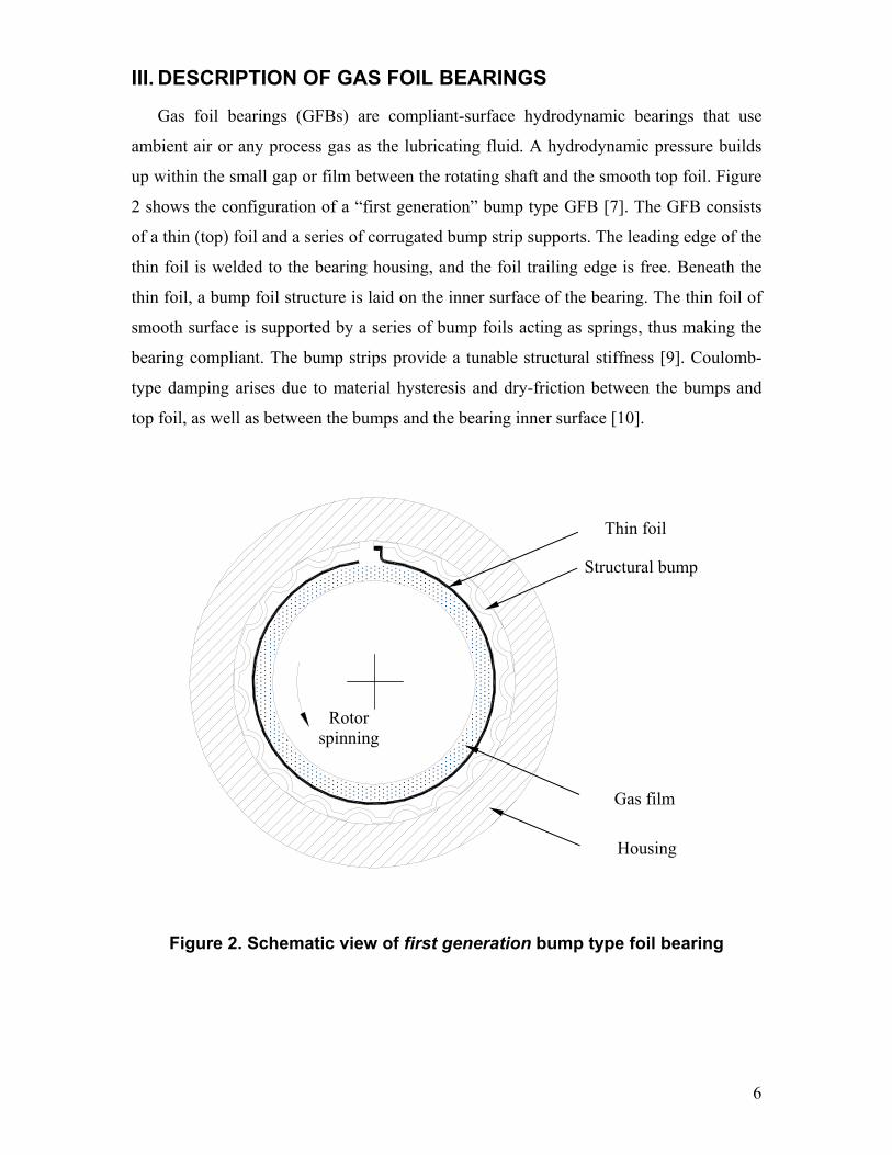
III. DESCRIPTION OF GAS FOIL BEARINGS

Gas foil bearings (GFBs) are compliant-surface hydrodynamic bearings that use

ambient air or any process gas as the lubricating fluid. A hydrodynamic pressure builds

up within the small gap or film between the rotating shaft and the smooth top foil. Figure

2 shows the configuration of a “first generation” bump type GFB [7]. The GFB consists

of a thin (top) foil and a series of corrugated bump strip supports. The leading edge of the

thin foil is welded to the bearing housing, and the foil trailing edge is free. Beneath the

thin foil, a bump foil structure is laid on the inner surface of the bearing. The thin foil of

smooth surface is supported by a series of bump foils acting as springs, thus making the

bearing compliant. The bump strips provide a tunable structural stiffness [9]. Coulomb-

type damping arises due to material hysteresis and dry-friction between the bumps and

top foil, as well as between the bumps and the bearing inner surface [10].

Figure 2. Schematic view of first generation bump type foil bearing

Housing

Structural bump

Thin foil

Gas film

Rotor spinning

7

The Reynolds equation describes the generation of the gas pressure (p) within the

film thickness (h). For an isothermal, isoviscous ideal gas this equation is

( ) ( )3 3 6 12

ph php pph ph Rx x z z x t

μ μ∂ ∂∂ ∂ ∂ ∂⎛ ⎞ ⎛ ⎞+ = Ω +⎜ ⎟ ⎜ ⎟∂ ∂ ∂ ∂ ∂ ∂⎝ ⎠ ⎝ ⎠

(1)

where (x, z) are the circumferential and axial coordinates on the plane of the bearing. The

pressure takes ambient value (pa) on the side boundaries of the bearing. The film

thickness (h) for a perfectly aligned journal is

( )cos cos( ) sin( )p p X Y dh c r e e w= − Θ −Θ + Θ + Θ + (2)

where c and rp are the assembled clearance and preload, respectively; and (eX, eY) are the

journal center displacements. w is the elastic deflection of the underlying support

structure, a function of the hydrodynamic pressure field and the material and geometric

characteristics of the support structure comprised of the top foil and the bump strip layers.

IV. MODELING OF FOIL SUPPORT STRUCTURE

IV.1 CONVENTIONAL SIMPLE ELASTIC FOUNDATION MODEL

Most published models for the elastic support structure in a GFB are based on the

original work of Heshmat et al. [9,12]. This analysis relies on several assumptions which

most researchers [10,13,14,18] also reproduce:

(1) The stiffness of a bump strip is uniformly distributed throughout the bearing

surface, i.e. the bump strip is regarded as a uniform elastic foundation.

(2) A bump stiffness is constant, independent of the actual bump deflection, not

related or constrained by adjacent bumps.

(3) The top foil does not to sag between adjacent bumps. The top foil does not have

either bending or membrane stiffness, and its deflection follows that of the bump.

With these considerations, the local deflection of a bump (wd) depends on the bump

structural stiffness (Kf) and the average pressure (δpA) across the bearing width, i.e.

8

d A fw p Kδ= (3)

where ( )0

1 LA ap p p dz

Lδ = −∫ , and pa is the ambient pressure beneath the foil.

Coupling of the simple model, Eq. (3), with the solution of Reynolds Eq. (1) is

straightforward, leading to fast computational models for prediction of the static and

dynamic force performance of GFBs, see [8-10] for example.

Presently, the simple foundation model is extended to account for and integrate with

the elastic deformation of the top foil. The top foil is modeled as a flat shell, i.e. without

curvature effects since the transverse deflections are roughly ~0.001 of the top foil

assembled radius of curvature. Two structural models for the top foil follow:

a) one-dimensional model which considers an axially averaged gas film pressure

acting along the top foil width and thus no structural deformation along the

bearing axial direction; and,

b) two-dimensional model which considers the whole gas pressure field acting on

the top foil with transverse deformations along the bearing circumferential and

axial directions.

The first model is simpler and less computationally intensive. Both top foil strutucal

models incorporate the bump strip layer as a series of linear springs, not connected with

each other. Interactions between adjacent bumps are altogether neglected, as is usual in

most predictive models. The stiffness of each bump is regarded as constant (irrespective

of the load) does denoting no change in the nominal or manufactured bump pitch.

IV.2 ONE DIMENSIONAL ELASTIC MODEL FOR TOP FOIL

In their extensive GFB experimental work, Ruscitto et al. [19] report relatively small

differences in axial gas film (minimum) thickness for heavily loaded conditions. This

means that an average pressure causes a uniform elastic deformation along the top foil of

width (L). Hence, a one dimensional structural model, with infinite stiffness along the

bearing width, may suffice to model the top foil, as shown in Figure 3. One end of the top

foil is fixed, i.e. with transverse deflection and rotation equal to nil; while the other end is

9

free. Figure 3 also shows the idealization of the 1D model with its degrees of freedom,

namely transverse deflections (w) and rotations (φ).

Figure 3. Configuration of top foil supported on a bump strip and its 1D structural model. Generalized displacements: 1

eu =w1, 2eu =φ1, 3

eu =w2, and 4eu =φ2

Figure 4 displays schematic representations of the actual and idealized structural

deformations for the top foil and adjacent bumps. In actual operation, the bumps are

flattened under the action of the acting pressure, the contact area with the top foil

increases, and this effect increases locally the stiffness of the top foil. Hence, an

anisotropic elastic model may compensate for the overestimation of top foil deflections

between adjacent bumps. Presently, the elastic modulus for the top foil (Et) is artificially

increased, E* = Et × Sfc, where (Sfc) as a stiffening factor in the circumferential direction.

Note that the curvature radius of the top foil deflected shape (sagging) cannot exceed that

of the original bumps shapes, thus suggesting the appropriate range of stiffening factors

for known GFB configurations.

lex

1eu 3

eu 2eu 4

eu

q(x)·L

w x (=RΘ)

Smooth Top Foil

Bump supports Weld

ΩR

ΩR

10

Figure 4. Schematic representations of deformations in actual and idealized top foil and bump strips

The top foil transverse deflection (w) along the circumferential axis (x) is governed

by the fourth order differential equation:

( )2 2

2 2d d wEI q x Ldx dx

⎛ ⎞= ⋅⎜ ⎟⎜ ⎟

⎝ ⎠ (4)

where E and I are the elastic modulus and moment of inertia, and q·L=(p-pa) ·L is the

distributed load per unit circumferential length. Note that Eq. (4) is the typical

formulation for the deflections of an Euler-like beam. Appendix A and reference [22]

detail the weak form of Eq. (4) when integrated over the domain of one finite element.

IV.3 TWO DIMENSIONAL MODEL FOR TOP FOIL

The second model regards the top foil as a two dimensional flat shell supported on

axially distributed linear springs located at every bump pitch, as shown in Figure 5.

Figure 6, graphs (a) and (b), depicts the membrane force (N), shear force (Q) and bending

moment (M) per unit element length, and external pressure difference (q=p-pa) acting on

(a) Foil deflections in actual GFBs (b) Foil deflections for equivalent model

∆wactual

∆wactual ≤ ∆wequiv

Kbump Kbump

∆wequiv“Sag” “Bump

flattened”

bump spring

Flexible Top foil

Pressure

11

the shell element OABC. The generic displacements are denoted as u, v and w along the x,

y and z directions, respectively [23].

Figure 5. Configuration of top foil supported on a bump strip and its 2D structural model

Smooth Top Foil

Bump supports Weld

ΩR

No. of finite elementsbetween bumps

Axially distributed linear spring

Fixed end

Thin Shell

Shell Length Shell width

Finite element

Shell thickness

12

(a) Normal plane (membrane) stresses

(b) Bending and shear stresses

Figure 6. Resultant membrane forces and bending moments per unit shell element length for a distributed load in the domain of a shell finite element

Timoshenko and Woinowsky-Krieger [23] detail the differential equations for the

general cases of deformation in a cylindrical shell. In the present structural configuration,

membrane or in-plane forces per unit element length (N) are negligible since the axial

(side) ends of the top foil are regarded as free (not constrained) and because the gas film

pressure acts normal to the top foil. Gas film shear forces between the film and top foil

z, w

y, v

x, u

xyxy

NN dx

x∂

+∂

xx

NN dx

x∂

+∂

yy

NN dy

y∂

+∂

yxyx

NN dy

y∂

+∂

xN

xyN

yxNyN

R

O A

B C dy

dx

q

dΘ

xyxy

MM dx

x∂

+∂

xx

MM dx

x∂

+∂

yy

MM dy

y∂

+∂

yxyx

MM dy

y∂

+∂

xM

xyM yxM

yM

R

xQ

yQ

yy

QQ dy

y∂

+∂

xx

QQ dx

x∂

+∂

q

z, w

y, v

x, u

dΘ

13

and dry-friction forces between the top foil and bumps underneath do induce membrane

forces. However, these are neglected for simplicity.

Presently, an anisotropic shell model will compensate the simplification. A stiffening

factor (Sfa) for the top foil elastic modulus (Et), i.e. Et* = Et × Sfa, in the axial direction

and a stiffening factor (Sfc) in the circumferential direction will prevent the

overestimation of the top foil deflections near the foil unconstrained (free) edges and

between adjacent discrete bump structures, respectively. The stiffening factors are

determined by trial and error!

Thus, the present analysis retakes the anisotropic, shear deformable plate model based

on first-order shear deformation theory. As given in [22], the governing equations are

0yx QQq

x y∂∂

+ − =∂ ∂

;

0yxxx

MMQ

x y∂∂

+ − =∂ ∂

;

0yx yy

M MQ

x y∂ ∂

+ − =∂ ∂

(5)

where

11 12yx

xM D Dx x

φφ ∂∂= +

∂ ∂; 12 22

yxyM D D

x yφφ ∂∂

= +∂ ∂

; 66yx

xyM Dy x

φφ ∂⎛ ⎞∂= +⎜ ⎟⎜ ⎟∂ ∂⎝ ⎠

55x xwQ Ax

φ ∂⎛ ⎞= +⎜ ⎟∂⎝ ⎠; 44y y

wQ Ay

φ⎛ ⎞∂

= +⎜ ⎟∂⎝ ⎠

(6)

and

( )3

111

12 2112 1tE h

Dν ν

=−

; ( )

312 2

1212 2112 1

tE hD

νν ν

=−

; ( )

32

2212 2112 1tE h

Dν ν

=−

; ( )

312

6612 2124 1tE h

Dν ν

=−

( )13

55132 1t

tE h

A kν

=−

; ( )

2344

232 1t

tE h

A kν

=−

(7)

xφ and yφ in Eq. (6) denote rotation angles about the y and x axes, respectively. ht, Eij, νij,

in Eq. (7) represent the shell thickness, anisotropic elastic modulii and Poisson’s ratios,

respectively [24]. kt (=5/6) is a shear correction coefficient, introduced to account for the

discrepancy between the distribution of transverse shear stresses of the first-order theory

and actual distribution [22].

14

Note that, in Eqs. (5-7), neglecting the deflections (w, yφ ) along the y axis leads to the

governing equations for Timoshenko’s beam theory [23]. Appendix B details the weak

form of Eqs. (5-7) when integrated over a two-dimensional finite element domain.

Figure 7 presents a four-node, shell element supported on an axially distributed linear

spring on one end, as taken from Fig. 5. lex, ley, and ht represent the element length, width,

and thickness, respectively. At each node, there are three degrees of freedom, a transverse

deflection and two rotations. Note that the axially distributed linear spring reacts only to

the transverse deflection, w.

Figure 7. Four-node, shell finite element supported on an axially distributed linear spring

Equation (8) below details the stiffness matrix [Ks] for one structural bump

supporting a top foil at one of its edges. This matrix is integrated into the shell element

stiffness matrix [Ke] given in Appendix B.

0 0 0 0 0 0 0 0 0 0 0 00 0 0 0 0 0 0 0 0 0 0 00 0 0 0 0 0 0 0 0 0 0 00 0 0 1 0 0 1/ 2 0 0 0 0 00 0 0 0 0 0 0 0 0 0 0 00 0 0 0 0 0 0 0 0 0 0 00 0 0 1/ 2 0 0 1 0 0 0 0 030 0 0 0 0 0 0 0 0 0 0 00 0 0 0 0 0 0 0 0 0 0 00 0 0 0 0 0 0 0 0 0 0 00 0 0 0 0 0 0 0 0 0 0 00 0 0 0 0 0 0 0 0 0 0 0

s lKK

⎡ ⎤⎢ ⎥⎢ ⎥⎢ ⎥⎢ ⎥⎢ ⎥⎢ ⎥⎢ ⎥⎢ ⎥⎡ ⎤ = ⎢ ⎥⎣ ⎦⎢ ⎥⎢ ⎥⎢ ⎥⎢ ⎥⎢ ⎥⎢ ⎥⎢ ⎥⎢ ⎥⎢ ⎥⎣ ⎦

for

1

1

1

2

2

2

3

3

3

4

4

4

x

y

x

ye

x

y

x

y

w

w

Uw

w

φφ

φφ

φφ

φφ

⎧ ⎫⎪ ⎪⎪ ⎪⎪ ⎪⎪ ⎪⎪ ⎪⎪ ⎪⎪ ⎪⎪ ⎪⎪ ⎪= ⎨ ⎬⎪ ⎪⎪ ⎪⎪ ⎪⎪ ⎪⎪ ⎪⎪ ⎪⎪ ⎪⎪ ⎪⎪ ⎪⎩ ⎭

(8)

where 0l f eyK K s l= × × ; s0 is the bump pitch and Kf, the bump stiffness per unit area, is

4

Axially distributed linear spring

Finite element1

3

2

x y

z

ley lex

h kl

15

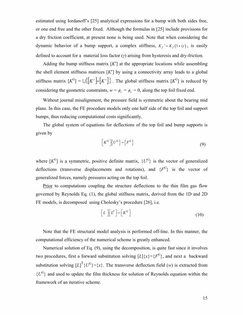
estimated using Iordanoff’s [25] analytical expressions for a bump with both sides free,

or one end free and the other fixed. Although the formulas in [25] include provisions for

a dry friction coefficient, at present none is being used. Note that when considering the

dynamic behavior of a bump support, a complex stiffness, ( )' 1f fK K iγ= + , is easily

defined to account for a material loss factor (γ) arising from hysteresis and dry-friction.

Adding the bump stiffness matrix [Ks] at the appropriate locations while assembling

the shell element stiffness matrices [Ke] by using a connectivity array leads to a global

stiffness matrix [KG] = [ ] [ ] se KK +U . The global stiffness matrix [KG] is reduced by

considering the geometric constraints, w = xφ = yφ = 0, along the top foil fixed end.

Without journal misalignment, the pressure field is symmetric about the bearing mid

plane. In this case, the FE procedure models only one half side of the top foil and support

bumps, thus reducing computational costs significantly.

The global system of equations for deflections of the top foil and bump supports is

given by

G G GK U F⎡ ⎤ =⎣ ⎦ (9)

where [KG] is a symmetric, positive definite matrix, UG is the vector of generalized

deflections (transverse displacements and rotations), and FG is the vector of

generalized forces, namely pressures acting on the top foil.

Prior to computations coupling the structure deflections to the thin film gas flow

governed by Reynolds Eq. (1), the global stiffness matrix, derived from the 1D and 2D

FE models, is decomposed using Cholesky’s procedure [26], i.e.

Note that the FE structural model analysis is performed off-line. In this manner, the

computational efficiency of the numerical scheme is greatly enhanced.

Numerical solution of Eq. (9), using the decomposition, is quite fast since it involves

two procedures, first a forward substitution solving [L]x=FG, and next a backward

substitution solving [L]TUG=x. The transverse deflection field (w) is extracted from

UG and used to update the film thickness for solution of Reynolds equation within the

framework of an iterative scheme.

T GL L K⎡ ⎤ ⎡ ⎤ ⎡ ⎤=⎣ ⎦ ⎣ ⎦ ⎣ ⎦ (10)

16

V. COMPARISONS OF PREDICTIONS TO PUBLISHED TEST DATA

V. 1 CONFIGURATION OF TEST GFB The validity of the analysis and computational program is assessed by comparison of

predictions to experimental data available in the open literature. Table 1 provides

parameters for the test foil bearing given in [19] and Figure 8 depicts the configuration of

the bump foil strip. The foil bearing is a “first generation” type with one 360º top foil and

one bump strip layer, both made of Inconel X-750. The top foil and bump layer are spot

welded at one end to the bearing sleeve. The other end of the top foil is free as well as the

end of the bump strip layer. The journal rotational direction is from the free end of the top

foil towards its fixed end.

Table 1 Design details of foil bearing, reference [19]

Bearing radius, R=D/2 19.05 mm (0.75 inch)

Bearing length, L 38.1 mm (1.5 inch)

Foil arc circumferential length, lx 120 mm (4.7 inch)

Radial journal travel, cJ (~ clearance) 31.8 μm (1.25 mil)

Top foil thickness, tt 101.6 μm (4 mil)

Bump foil thickness, tb 101.6 μm (4 mil)

Bump pitch, s 4.572 mm (0.18 inch)

Half bump length, l0 1.778 mm (0.07 inch)

Bump height, hb 0.508 mm (0.02 inch)

Number of bumps*, Nb 26

Bump foil Young’s modulus, E 214 Gpa (31 Mpsi)

Bump foil Poisson’s ratio, ν 0.29

All tests in [19] were performed with air at ambient condition. Because the bearing

clearance for the test bearing was unknown, the journal radial travel ( Jc ) was measured

by performing a static load-bump deflection test. Details of the measuring procedure are

described in [19]. The journal radial travel refers to the displacement where the journal

* The number of bumps (Nb) is calculated by dividing the foil arc circumferential length (lx) by the bump pitch (s).

17

can sway under an arbitrary static load condition†. Hence, in [19], the journal radial travel

(2 Jc =63.6 μm) is obtained from the total displacement of the bearing when a 0.9 kg (2

lb) load was applied first downward, and then upwards.

Figure 8. Configuration of top foil and bump foil strips

The structural stiffness per unit area (Kf) is estimated from Iordanoff’s formulae [25].

The bump pitch (s) is regarded as constant and the interaction between bumps is

neglected. The calculated structural stiffness coefficients per unit area for a free-free ends

bump and a fixed-free end bump are Kff = 4.7 GN/m3 and Kfw = 10.4 GN/m3, respectively.

V.2 MINIMUM FIILM THICKNESS AND JOURNAL ATTITUDE ANGLE

The GFB computational tools integrating the 1D and 2D finite element top foil

structural models, as well as the earlier simple elastic foundation model, predict the static

and dynamic force performance of the test GFB.

The 2D FE model uses a mesh of 78 and 10 elements in the circumferential and axial

directions, respectively. The same mesh size is used for the finite difference numerical

scheme solving Reynolds Eq. and calculating the hydrodynamic gas film pressure. On the

other hand, the 1D FE model uses a mesh of 78 elements in the circumferential direction.

A mesh of 78 and 10 elements, in the circumferential and axial directions, respectively, is

used to analyze the gas film pressure. Predictions using the simple elastic foundation

model, for a mesh of 90 and 10 elements in the circumferential and axial directions,

respectively, are directly taken from [18].

† This ad-hoc procedure reveals the region where the foil structure is apparently very “soft.”

tt

tb

l0

s

hb

18

Top foil stiffening factors Sfc= 4 and Sfa= 1 in the circumferential and axial directions,

respectively, were obtained through parametric studies based on the recorded test data in

[19]. In the 2D FE model, foil deflections along its edges are calculated using the axial

upstream pressures modified by the local Peclet number [27], a procedure based on

physical reasoning which improves the accuracy in the prediction in the gas film

thickness. Note that FE predictions underestimate the top foil deflections when compared

to the test data in [19]. This behavior is caused by the omission of membrane stresses in

the current model.

Figure 9 presents the minimum film thickness versus applied static load for operation

at shaft speeds equal to (a) 45,000 rpm and (b) 30,000 rpm. The graphs includes the test

data [19], and predictions for three increasingly complex structural models; namely, the

simple elastic foundation, 1D top foil acted upon an axially averaged gas pressure, and

the 2D top foil with circumferential stiffening. In the tests, film thicknesses were

recorded at both the bearing mid-plane and near the bearing exit-planes, i.e. 1.6 mm from

the bearing axial ends. The 2D model predictions show minimum film thicknesses along

the bearing mid-plane and near the bearing edges, i.e. 1.9 mm away. Both the simple

elastic model and the 1D FE model predictions show a film thickness not varying across

the bearing width since the models rely on an axially averaged pressure field.

In general, all model predictions agree fairly with the test data [19]. Incidentally, the

measurement errors reported in [19] render a precision uncertainty of ~15 % for film

thickness.

19

0

10

20

30

0 50 100 150 200

Static load [N]

Min

imum

film

thic

knes

s [μ

m]

Centerline test point (Ruscitto, et al., 1978)Endline test point (Ruscitto, et al., 1978)Centerline prediction (2D FE model)Endline prediction (2D FE model)Avg. film prediction (1D FE model)Avg. film prediction (simple model)

Test data (centerline)

Prediction(centerline, 2D)

Test data (endline) Prediction

(endline, 2D)

Prediction (1D)

Prediction (simple model)

(a) 45,000 rpm

0

10

20

30

0 50 100 150 200

Static load [N]

Min

imum

film

thic

knes

s [μ

m]

Centerline test point (Ruscitto, et al., 1978)Endline test point (Ruscitto, et al., 1978)Centerline prediction (2D FE model)Endline prediction (2D FE model)Avg. film prediction (1D FE model)Avg. film prediction (simple model)

Test data (centerline)

Prediction(centerline, 2D)

Test data (endline) Prediction

(endline, 2D)

Prediction (1D) Prediction

(simple model)

(b) 30,000 rpm

Figure 9. Minimum film thickness versus static load. Predictions from three foil structural models and test data [19]

20

Over the whole range of static loads, 2D top foil model predictions overestimate the

minimum film thickness at the bearing mid-plane, and slightly underestimate this

parameter at the top foil edge. The discrepancies are due to membrane forces preventing

the extension of the top foil. Membrane forces force a uniform deflection along the

bearing width, in particular for heavy static loads. This effect is most notable for a

uniform pressure field along the bearing width. See Fig. 10 for a comparison of the

axially averaged minimum film thickness calculated from the 2D model and the test data

(simple arithmetic average of film thicknesses recorded at the bearing mid-plane and near

edges). The predictions correlate very well with the test data at 45,000 rpm and 30,000

rpm, respectively.

The assumption of an axially uniform minimum film thickness in the 1D top foil

model results in a significant reduction of computational costs, as discussed in more

detail later. More importantly, the 1D top foil model predictions show the best correlation

to the collected experimental results. The simpler model predictions slightly overestimate

the minimum film thickness, especially for heavy static loads.

0

10

20

30

0 50 100 150 200

Static load [N]

Min

imum

film

thic

knes

s [μ

m]

45,000 rpm avg. test point (Ruscitto, et al., 1978)

45,000 rpm avg. prediction (2D FE model)

30,000 rpm avg. test point (Ruscitto, et al., 1978)

30,000 rpm avg. prediction (2D FE model)

Avg. test data

Avg. prediction

Figure 10. Axially averaged minimum film thickness versus static load. Predictions from 2D top foil model and test data [19]

Figure 11 depicts the journal attitude angle versus applied static load for speeds equal

to (a) 45,000 rpm and (b) 30,000 rpm, respectively. The graph includes predictions from

21

the three structural models and test data [19]. All model predictions slightly

underestimate the test data above 60 N. The notable discrepancy between predictions and

test results for static loads below 60 N can be attributed to foil bearing fabrication

inaccuracy [19]. The 1D top foil structural model predictions demonstrate the best

correlation to the test data. In general, all model predictions agree well with the test data.

Figure 12 presents the predicted journal eccentricity versus applied static load for

operation at a rotational speed of 45,000 rpm. Reference [19] does not provide test data

regarding journal eccentricity. For static loads above 60N, i.e. specific load of 41.4 kPa

(6 psi), where the journal eccentricity exceeds the nominal clearance (cJ), the journal

displacement is proportional to the applied load. The simple elastic foundation model

predicts an ultimate static stiffness KG=5.2×106 N/m, which is nearly identical to the

structural stiffness KS =5.3×106 N/m. See [18] for a comparison of the journal eccentricity

predicted using the simple model to the structural deflection for load contact without

journal spinning. Similar trends in predicated journal eccentricity are evident for the 1D

and 2D top foil structural models. However, for heavy static loads, the 2D top foil model

shows a slightly larger eccentricity since the top foil, being flexible, “sags” in between

adjacent bumps.

0

10

20

30

40

50

60

0 50 100 150 200

Static load [N]

Jour

nal a

ttitu

de a

ngle

[deg

]

Test point (Ruscitto, et al., 1978)

Prediction (2D FE model)

(1D FE model)

(simple model)

Test data

Prediction(2D)

Prediction (1D) Prediction

(simple model)

(a) 45,000 rpm

22

0

10

20

30

40

50

60

0 50 100 150 200

Static load [N]

Jour

nal a

ttitu

de a

ngle

[deg

]

Test point (Ruscitto, et al., 1978)

Prediction (2D FE model)

(1D FE model)

(simple model)

Test data

Prediction(2D)

Prediction (1D) Prediction

(simple model)

(b) 30,000 rpm

Figure 11. Journal attitude angle versus static load. Predictions from three foil structural models and test data [19]

0.00

20.00

40.00

60.00

0 50 100 150 200

Static load [N]

Jour

nal e

ccen

tric

ity [μ

m]

2D FE model

1D FE model

Simple model

1D FE modelSimple model

2D FE model

Radial journal travel, c J = 31.8 µm

KG = 5.2 MN/m

Figure 12. Journal eccentricity versus static load at 45 krpm, Predictions from three foil structural models for GFB in [19]

23

Figure 13 displays the predicted dimensionless pressure field (p/pa) and the

corresponding film thickness derived from the 2D top foil structural model. A static load

of 200 N, specific pressure = 138 kPa (20 psi), acts on the rotor operating at a speed of

45,000 rpm. The hydrodynamic film pressure builds up within the smallest film thickness

region. During operation, the top foil could detach, not allowing for sub-ambient

pressures, i.e. p ≥ pa. For the heavily loaded condition (200 N) and due to the bearing

inherent compliance, the model prediction shows a large circumferential region of

uniform minimum film. The film thickness is nearly constant along the bearing axial

length except near the axial edges, as in the experiments [19]. The softness of the top foil

in between individual bumps, as shown in the film thickness field causes the local

pressure field to sag between consecutive bumps, i.e. the appearance of a “ripple” like

effect.

24

0

180

360

1

1.5

2

2.5

3

3.5

Dim

ensi

onle

ss p

ress

ure

[ p/p

a]

Circumferential location [deg]

(a) Pressure field

0

180

360

0

20

40

60

80

100

120

Film

thic

knes

s [μ

m]

Circumferential location [deg]

(b) Film thickness field

Figure 13. Predicted (a) dimensionless pressure field and (b) film thickness field from 2D top foil structural model. Static load: 200 N, rotor speed: 45 krpm. Bearing configuration given in [19]

25

Figure 14 presents the predicted film thickness versus circumferential location for the

1D top foil model and the measured film thickness [19] for a static load of 134.1 N and

rotor speed of 30 krpm. Along the zone of smallest film thickness, the predictions match

very well with the test data. Recall that the model does not account for the interaction

between adjacent bumps, thus showing a slight difference in the pitch of the ripple shapes.

Note that the test GFB has a nearly constant film thickness along the bearing axial length

(Δh < 1μm) for both load and speed conditions, as shown in Fig 9 (b).

Although the test GFB has a largely unknown radial clearance, due to a fabrication

inaccuracy, and its nominal bearing clearance is experimentally determined through a

simple load-deflection test, the comparisons demonstrate a remarkable correlation

between predictions and test data in the region of minute, nearly uniform, film thickness.

These comparisons validate the 1D top foil model for accurate prediction of GFB static

load performance.

Figure 14. Film thickness versus angular location at bearing mid-plane. Prediction from 1D top foil model and test data [19]. Static load: 134.1 N. Rotor speed: 30 krpm

0 50 0 100 0 150 0 200 0 250 0 300 0 350 0

Film

thic

knes

s [µm

]

0

40

80

120

160

0 90 180 270 360 Angular location [deg]

Active bumps region Test data

Prediction

26

V. 3 PREDICTED STIFFNESS AND DAMPING FORCE COEFFICEINTS

To date there is no published experimental data on GFB force coefficients, stiffness

and damping.

Figure 15 displays the bearing stiffness coefficients versus excitation frequency as

determined by the three structural support models. A static load of 150 N, i.e. specific

load of 1 bar (15 psi), is applied at 45,000 rpm. Synchronous excitation corresponds to a

frequency of 750 Hz. The results correspond to a negligible structural loss factor, γ = 0.0,

known to have an insignificant effect on the direct stiffness coefficients [10]. The direct

stiffness coefficients (KXX, KYY) increase with excitation frequency due to the “hardening”

of the gas film. All models predict very similar direct stiffness coefficients.

The simple elastic foundation model predicts the largest direct stiffness, KXX, while

the 2D top foil model renders the smallest. The “sagging” effect of the top foil in

between adjacent bumps in the 1D and 2D FE models is thought to reduce slightly the

bearing stiffness KXX. All predictions of cross-coupled stiffness coefficients show positive

values. Note that cross-coupled stiffness coefficients with same sign do not have

destabilizing effects [28]. The 1D top foil model predicts the largest KXY and the smallest

KYX. The 2D model predicts the smallest KXY, while the simple model predicts the largest

KYX. All model predictions demonstrate much greater direct stiffnesses, KXX and KXX, than

cross-coupled stiffnesses, KXY and KYX. Note that the difference in vertical axis scales in

Figure 15(a-c).

27

0

1

2

3

4

5

6

0 300 600 900 1200 1500Excitation frequency [Hz]

Dire

ct s

tiffn

ess

coef

ficie

nt [M

N/m

]

Simple model

K XX

K YY

1D FE model

2D FE model

(a) KXX, KYY

0

0.2

0.4

0.6

0.8

1

0 300 600 900 1200 1500

Excitation frequency [Hz]

Cro

ss-c

oupl

ed s

tiffn

ess

coef

ficie

nt [M

N/m

]

Simple model

K XY

1D FE model

2D FE model

(b) KXY

28

0

0.2

0.4

0.6

0.8

1

0 300 600 900 1200 1500

Excitation frequency [Hz]

Cro

ss-c

oupl

ed s

tiffn

ess

coef

ficie

nt [M

N/m

]

Simple model

K YX

1D FE model

2D FE model

(c) KYX

Figure 15. Predicted GFB stiffness coefficients versus excitation frequency for three structural models. Rotor speed: 45 krpm, Static load: 150 N. Structural loss factor γ = 0.0.

29

Figure 16 displays predicted damping coefficients versus excitation frequency as

determined from the three structural models. Static load and rotor speed are as in the last

figure. The structural loss factor γ = 0.4 represents a hysteresis damping effect in the

bump strip layer. With a structural loss factor (γ = 0.4), the direct damping coefficients

(CXX, CYY) increase significantly when compared to those for γ = 0.0, i.e. without material

damping. Regardless of the structural loss factor, the 2D top foil model predicts the

smallest direct damping coefficients (CXX, CYY). The simple elastic foundation model

prediction shows the largest coefficients, except for excitation frequencies lower than 500

Hz, where the 1D FE model predicts the largest CXX and CYY for a null loss factor (γ = 0).

Predictions of cross-coupled damping coefficients, CXY and CYX, do not show a

discernible difference among the three models. Generally, cross-coupled damping

coefficients (CXY, CYX) decrease in magnitude as the excitation frequency increases. Note

that the vertical axes of Figs. 16 (a) and 16 (b) show a log scale, while Figs. 16 (c) and 16

(d) show a linear scale along the vertical axes.

All model predictions demonstrate much greater direct damping, CXX and CXX, than

cross-coupled damping, CXY and CYX. In particular, for γ = 0.4, note the rapid reduction in

direct damping as the excitation frequency increases.

30

10

100

1000

10000

0 300 600 900 1200 1500

Excitation frequency [Hz]

Dire

ct d

ampi

ng c

oeffi

cien

t [N

-s/m

]

Simple model

C XX

γ = 0.4

1D FE model

2D FE model

γ = 0.0

(a) CXX

10

100

1000

10000

0 300 600 900 1200 1500

Excitation frequency [Hz]

Dire

ct d

ampi

ng c

oeffi

cien

t [N

-s/m

]

Simple

C YY

γ = 0.41D FE model

2D FE modelγ = 0.0

(b) CYY

31

-0.2

0

0.2

0.4

0 300 600 900 1200 1500

Excitation frequency [Hz]

Cro

ss-c

oupl

ed d

ampi

ng c

oeffi

cien

t [kN

-s/m

]

Simple model

C XY

γ = 0.4

1D FE model

2D FE model

γ = 0.0

(c) CXY

-0.2

0

0.2

0.4

0 300 600 900 1200 1500

Excitation frequency [Hz]

Cro

ss-c

oupl

ed d

ampi

ng c

oeffi

cien

t [kN

-s/m

]

Simple model

C YX

γ = 0.4

1D FE model2D FE model

γ = 0.0

(d) CYX

Figure 16. Predicted GFB damping coefficients versus excitation frequency for three structural models. Rotor speed: 45 krpm, Static load: 150 N. Structural loss factors, γ = 0.0 and 0.4

32

VI. COMPUTATIONAL TIME

In the present study, all analyses were conducted in a personal computer, Pentium® 4

processor (2.40 GHz CPU). The 1D structural model analysis requires much less

computational time than the 2D model, due to a reduction in the degrees of freedom.

While the 2D top foil model has 2,547 degrees of freedom, the 1D FE model has only

156. Therefore, in a particular case, the time to complete the 2D model analysis is ~10

seconds, while the 1D structural model analysis takes less than 1 second.

The perturbation analysis for calculation of force coefficients and implementing the

FE stiffness matrices increases the computational cost as compared to the performance of

the simple elastic foundation model analysis. For example, to find the static journal

eccentricity and the synchronous force coefficients for an applied load of 50 N at 45,000

rpm, the 1D and 2D FE structural models need ~14 seconds and ~180 seconds,

respectively, while the simpler model takes 9 seconds. Thus, the introduction of the 1D

and 2D top foil structural models into the GFB predictive computational code increases

the computational cost by 50% and 2000%, respectively. Note that the increase in

computational time depends mainly on the number of degrees of freedom in the FE

structure models.

33

VII. EFFECT OF MECHANICAL PRELOAD ON THE FORCED PERFORMANCE OF A GFB

Machined preloads in fluid film journal bearings aim to enhance the hydrodynamic

wedge to generate a pressure field that produces a centering stiffness even in the absence

of an applied static load [29]. The easiest way to introduce a preload into a GFB is by

inserting metal shims underneath a bump strip and in contact with the bearing housing

[30], as shown in Figure 17(a). The bump strip layers can also be manufactured with

varying bump heights to introduce a preload more akin to those in a multiple lobe rigid

surface bearing, see Figure 17(b). This second procedure is costly and probably

inaccurate.

Figure 17. Schematic views of gas foil bearing with (a) shims and (b) with machined preloads

For analysis purposes, a GFB is construed as a “three lobe” configuration. Table 2

presents the material and dimensional characteristics of the bearing studied. The nominal

clearance of the GFB equals 32 μm. Three shims of thickness 16 μm (~ 0.5 ×c) are

inserted at the circumferential locations 60º, 180º, and 360º. Hence, the mechanically

modified GFB has a dimensionless preload and offset ratio equal to 0.50 and 0.5,

respectively. Design details for the top foil and the bump layer in GFBs are identical to

those presented in Table 1. Predictions, derived from the uniform elastic foundation

(a)

Ω

Shim

Θ (b) Θ

Ω

Machined mechanical preload

34

model and from the 1D top foil model, show differences in performance characteristics

for a GFB with and without the mechanical preload, i.e. simple GFB.

Table 2 Geometry of foil bearing with mechanical preload (shims)

Bearing radius, R=D/2 19.05 mm (0.75 inch)

Bearing length, L 38.1 mm (1.5 inch)

Top foil arc circumferential length, lx 120 mm (4.7 inch)

Radial journal travel, cJ (~ clearance) 31.8 μm (1.25 mil)

Lobe arc angle 120 º

Shim arc angle* 40 º

Preload ratio**, rp/cJ 0.5

Preload offset ratio 0.5

Shim thickness, ts 16 μm (0.63 mil)

Number of shims, Ns 3

Shim material Inconel X-750 * ~13 mm length in the circumferential direction.

** The clearance (c) for a GFB with preload uses the shim thickness. The nominal gap between the top

foil and shaft follows the simple relationship ( ) ( )θθ 3cos24

3 PJ

rcc += for θ E 0, 2π.

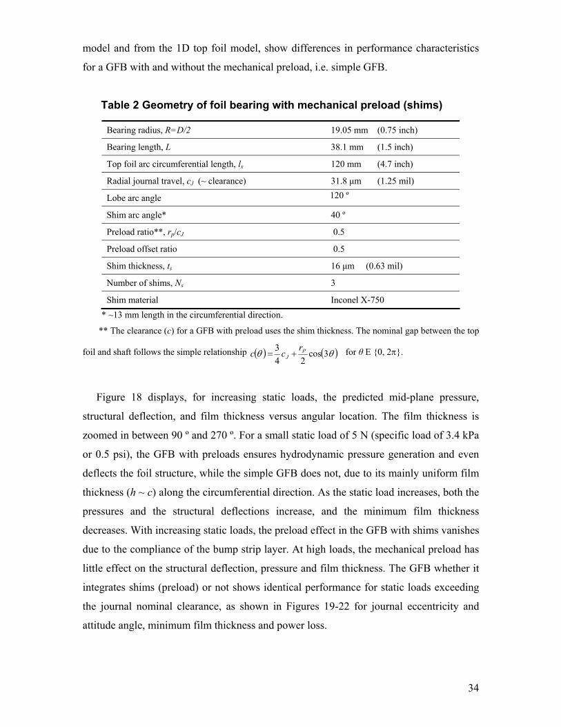
Figure 18 displays, for increasing static loads, the predicted mid-plane pressure,

structural deflection, and film thickness versus angular location. The film thickness is

zoomed in between 90 º and 270 º. For a small static load of 5 N (specific load of 3.4 kPa

or 0.5 psi), the GFB with preloads ensures hydrodynamic pressure generation and even

deflects the foil structure, while the simple GFB does not, due to its mainly uniform film

thickness (h ~ c) along the circumferential direction. As the static load increases, both the

pressures and the structural deflections increase, and the minimum film thickness

decreases. With increasing static loads, the preload effect in the GFB with shims vanishes

due to the compliance of the bump strip layer. At high loads, the mechanical preload has

little effect on the structural deflection, pressure and film thickness. The GFB whether it

integrates shims (preload) or not shows identical performance for static loads exceeding

the journal nominal clearance, as shown in Figures 19-22 for journal eccentricity and

attitude angle, minimum film thickness and power loss.

35

Figure 18. Dimensionless mid-plane pressure, structural deflection, and film thickness versus angular location for GFB with and without mechanical preload. Rotor speed: 45 krpm

-10

0

10

20

30

40

50

60

70

80

0 120 240 360

Stru

ctur

al d

efle

ctio

n [μ

m]

W= 300 N

W= 5 N

W= 150 NSimple GFB 3 lobe GFB

Structural deflection

0

20

40

60

80

100

120

140

0 120 240 360Angular location [deg]

Film

thic

knes

s [μ

m]

W= 300 N

W= 5 NW= 150 N

Simple GFB 3 lobe GFB

0

10

20

30

40

50

90 120 150 180 210 240 270Angular location [deg]

Film

thic

knes

s [μ

m]

W= 300 N

W= 5 N

W= 150 N

Simple GFB 3 lobe GFB

Film thickness (loaded zone)

1

10

0 120 240 360

Dim

ensi

onle

ss p

ress

ure,

p/p

a[-]

W= 300 N

W= 5 N

W= 150 N

Ω

X

Y

Θ

Simple GFB 3 lobe GFB

Θ

Ω

X

Y

Film pressure

36

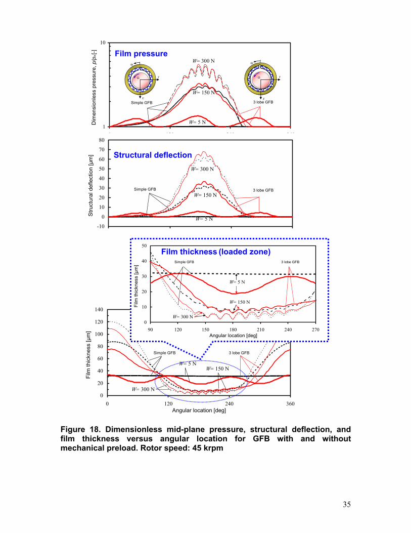
Figure 19 depicts the GFB journal eccentricity versus static load applied along the X

direction. With a mechanical preload, the GFB shows a linear relationship between load

and journal position, i.e. a constant and uniform stiffness, since the gas film is stiffer even

at low loads. The opposite behavior is evident for the GFB without shims, i.e. the journal

eccentricity is not proportional to the applied load due to the softness of the gas film. For

large loads, a linear behavior is notorious for journal eccentricities exceeding the bearing

nominal clearance, c = 31.8 μm. The GFB with mechanical preload leads to consistently

smaller journal static displacements than the simple GFB. From Figure 19, the difference

between eccentricities is approximately equal to the mechanical preload, 16 μm; in

particular at large loads.

0

20

40

60

80

0 50 100 150 200 250 300

Static load [N]

Jour

nal e

ccen

trici

ty [μ

m]

Ω

X

Y

Θ

Simple GFB

3 lobe GFB

Nominal bearing clearance, c =31.8 μm

Θ

Ω

X

Y

Figure 19. Journal eccentricity versus static load for GFB with and without mechanical preload. Rotor speed: 45,000 rpm

37

0

20

40

60

0 50 100 150 200 250 300

Static load [N]

Jour

nal a

ttitu

de a

ngle

[deg

] Ω

X

Y

Θ

Simple GFB

3 lobe GFB

Θ

Ω

X

Y

Figure 20. Journal attitude angle versus static load for for GFB with and without mechanical preload. Rotor speed: 45,000 rpm

0

10

20

30

0 50 100 150 200 250 300

Static load [N]

Min

imum

film

thic

knes

s [μ

m]

Ω

X

Y

Θ

Simple GFB

3 lobe GFB

Θ

Ω

X

Y

Figure 21. Minimum film thickness versus static load for GFB with and without mechanical preload. Rotor speed: 45,000 rpm

38

0

0.01

0.02

0.03

0.04

0.05

0.06

0.07

0 50 100 150 200 250 300

Static load [N]

Pow

er lo

ss [k

W]

Ω

X

Y

Θ

Simple GFB

3 lobe GFB

Θ

Ω

X

Y

Figure 22. Drag power loss versus static load for GFB with and without mechanical preload. Rotor speed: 45,000 rpm

Figure 23 shows, for operation at 45 krpm, the synchronous stiffness and damping

coefficients versus static load for the studied GFB, with and without a preload (shims).

The predictions correspond to a structural loss factor γ = 0.2. In figures 23(a), the thick

solid line with squares represents the bearing structural stiffness coefficient, Kstruc. The

GFB with preload, as expected, has larger direct stiffness coefficients, KXX and KYY, than

the simple GFB, in particular at low static loads. The cross-coupled stiffness coefficients,

KXY and KYX, for both bearing configurations are comparable in magnitude.

For the GFB with preload the direct damping coefficients, CXX and CYY shown in

Figure 23(b), increase dramatically for low static loads. The damping increases effect is

more pronounced for CXX than for CYY, and due to the reduced local clearance because of

the shims. The magnitudes of cross-coupled damping coefficients, CXY and CYX, increase

slightly for small static loads. In brief, the GFB with mechanical preload shows a

significant increase in direct synchronous stiffness and damping coefficients for low

static loads. This obvious advantage becomes less noticeable for large static loads.

39

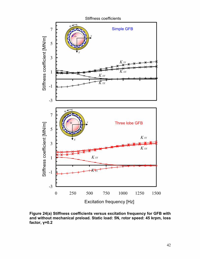
Figure 24 displays the stiffness and damping coefficients versus excitation

frequency. The operating speed is 45 krpm and small static load, just 5 N, applied along

the X direction. As the excitation frequency increases, the direct stiffness coefficients,

KXX and KYY, increase due to the hardening of the hydrodynamic gas film. Most

importantly, while the cross-coupled stiffness KXY > KXX and KYY at low frequencies in the

simple GFB; KXX increases for the bearing with preload and is larger than the cross

coupled stiffness. Direct damping coefficients, CXX and CYY, for the bearing with preload

are larger at low frequencies than those of the simple GFB. The differences become

minimal as the excitation frequency increases.

40

-1

0

1

2

3

4

5

6

Syn

chro

nous

stif

fnes

s co

effic

ient

[MN

/m]

Ω

X

Y

Θ

K struc

K XX K YY

K XY

K YX

-1

0

1

2

3

4

5

6

0 50 100 150 200 250 300

Static load [N]

Syn

chro

nous

stif

fnes

s co

effic

ient

[MN

/m]

K struc

K XX

K YY

K XY

K YX

Θ

Ω

X

Y

Figure 23a. Synchronous stiffness coefficients versus static load for GFB with and without preload. Rotor speed: 45,000 rpm, loss factor, γ=0.2

Simple GFB

Three lobe GFB

Synchronous stiffness coefficients

41

-200

-100

0

100

200

300

400

500

Syn

chro

nous

dam

ping

coe

ffici

ent [

N-s

/m]

Ω

X

Y

Θ

C XX

C YY

C XY

C YX

-200

-100

0

100

200

300

400

500

0 50 100 150 200 250 300

Static load [N]

Syn

chro

nous

stif

fnes

s co

effic

ient

[MN

/m]

C XX

C YY

C XY

C YX

Θ

Ω

X

Y

Figure 23b. Synchronous damping coefficients versus static load for GFB with and without preload. Rotor speed: 45,000 rpm, loss factor, γ=0.2

Simple GFB

Three lobe GFB

Synchronous damping coefficients

42

-3

-1

1

3

5

7

Stif

fnes

s co

effic

ient

[MN

/m] Ω

X

Y

Θ

K XX

K YY

K XY

K YX

-3

-1

1

3

5

7

0 250 500 750 1000 1250 1500

Excitation frequency [Hz]

Stif

fnes

s co

effic

ient

[MN

/m]

K XX

K YY

K XY

K YX

Θ

Ω

X

Y

Figure 24(a) Stiffness coefficients versus excitation frequency for GFB with and without mechanical preload. Static load: 5N, rotor speed: 45 krpm, loss factor, γ=0.2

Simple GFB

Three lobe GFB

Stiffness coefficients

43

-600

-400

-200

0

200

400

600

800

Dam

ping

coe

ffici

ent [

N-s

/m] Ω

X

Y

Θ

C XX

C YY

C XY

C YX

-600

-400

-200

0

200

400

600

800

0 250 500 750 1000 1250 1500

Excitation frequency [Hz]

Dam

ping

coe

ffici

ent [

N-s

/m]

C XX

C YY

C XY

C YX

Θ

Ω

X

Y

Figure 24(b) Damping coefficients versus excitation frequency for GFB with and without mechanical preload. Static load: 5N, rotor speed: 45 krpm, loss factor, γ=0.2

Simple GFB

Three lobe GFB

Damping coefficients

44

The energy imparted to the rotor (per period of motion) is,

( ) ( )cycle X Y X YE F dX F dY F Xdt F Ydt= + = +∫ ∫ & &

where X XX XY XX XY

Y YX YY YX YY

F K K C CX XF K K C CY Y

⎧ ⎫⎧ ⎫ ⎡ ⎤ ⎡ ⎤⎧ ⎫ ⎪ ⎪= − −⎨ ⎬ ⎨ ⎬ ⎨ ⎬⎢ ⎥ ⎢ ⎥⎪ ⎪⎩ ⎭⎩ ⎭ ⎣ ⎦ ⎣ ⎦ ⎩ ⎭

&

& (8)

Consider rotor motions describing a forward whirl circular orbit, of amplitude A

and frequency ω, i.e., ( )cosX A tω= and ( )sinY A tω= . Hence [31]:.

( ) ( ) cycle cycle XX YY XY YXE Ar C C K Kω= − + − −

where 2cycleAr Aπ=

(9)

The energy dissipated ( cycleE− ) by the GFB uses the predictions of stiffness and

damping coefficients for increasing frequencies and static loads. Figure 25 shows the

predicted energy dissipated per unit area of circular orbit for a GFB with and without

mechanical preload operating at 45,000 rpm (750 Hz). For low loads, 5N and 50 N, the

GFB with and without shims are unstable (negative dissipated energy) and with identical

threshold frequencies, namely 270 Hz and 350 Hz, respectively. The threshold frequency

notes when the energy turns positive, thus actually dissipating energy to reduce vibrations.

Regardless of preload, the GFB is stable for the largest load (150 N) over the entire

frequency range. Although there is not a significant difference in the threshold frequency

(ωthreshold), the threshold speed of instability (Ωthreshold) will increase when including a

mechanical preload (shim) because the bearing direct stiffness will increase the system

natural frequency (ωn) of the rigid rotor-GFB system, i.e., Ωthreshold = ωn/WFR. This

observation is strictly applicable to a rigid rotor-bearing system.

45

-3

-2

-1

0

1

2

3

10 100 1000 10000

Excitation frequency [Hz]

Ene

rgy

diss

ipat

ed p

er u

nit a

rea

circ

ular

orb

it [M

N/m

]

3 lobe GFB

Ω

X

Y

Θ

Cylindrical GFB

Θ

X

Y

5 N

50 N

150 N

Figure 25. Energy dissipated by a GFB with and without mechanical preload for increasing static loads. Rotor speed: 45 krpm (750 Hz), loss factor, γ=0.2

ωthreshold=350 Hz ωthreshold=270 Hz

ωsync=750 Hz

46

VIII. CLOSURE

Conventional analyses of GFBs neglect the elasticity of the top foil and consider the

bump strip layers support structure as an elastic foundation with uniform stiffness. This

simple model has been most useful for decades; however, stringent applications of gas

bearings into commercial oil-free turbomachinery demands the development of more

realistic models to better engineer them as reliable supports.

Presently, the report introduces two finite element models for the top foil elastic

structure. The simplest FE model assumes the top foil as a 1D beam with negligible

deflections along the axial coordinate, i.e. infinitely stiff and acted upon by a uniformly

distributed pressure field. The second FE model, 2D, takes the top foil as a flat shell with

anisotropic material properties. The underlying bumps modeled as a uniform elastic

foundation along the edge of a typical finite element representing a top foil, are directly

integrated into a global stiffness matrix that relates the top foil (and bumps) deflections to

applied gas film pressure or contact pressure, depending on the operating condition. The

decomposition of the symmetric stiffness matrix into upper and lower triangular parts is

performed off-line and prior to computations coupling it to the gas bearing analysis. The

procedure greatly enhances the computational efficiency of the numerical scheme.

Predictions of load capacity, attitude angle, and minimum film thickness versus

journal speed are obtained for a gas foil bearing tested decades ago [19]. This reference is,

to date, the only one with full details on bearing configuration and structural properties.

The predictions presented correspond to three models: (a) simplest elastic foundation

with no accounting for top foil structure, (b) 1D FE model with top foil as a thin beam,

and (c) 2D FE model with top foil as a shell.

2D FE model predictions overestimate the minimum film thickness at the bearing

centerline, but underestimate it at the bearing edges. Predictions from the 1D FE model

compare best to the limited tests data; reproducing closely the experimental

circumferential profile of minimum film thickness reported in [19]. The 1D top foil

model is to be preferred due to its low computational cost. The FE models predictions

show local ripples in the top foil supported in between bumps. The ripples are a pathway

for gas to escape out of the bearing, thus decreasing the hydrodynamic pressure and

diminishing the bearing load carrying capacity.

47

Predicted stiffness and damping coefficients versus excitation frequency show that

the two FE top foil structural models result in slightly lower direct stiffness and damping

coefficients than those from the simple elastic foundation model.

A three lobe GFB with mechanical preloads, introduced by inserting shims

underneath the bump strips, is analyzed using the 1D FE structural model. Predictions

show the mechanical preload enhances the load capacity of the gas foil bearing for

operation at low loads and low shaft speeds. Energy dissipation, a measure of the bearing

ability to ameliorate vibrations, is not affected by the preload induced although the direct

stiffness of the bearings is of importance for operation at high speeds with low load

conditions. Mechanical preload has no effect on the static and dynamic forced

performance of GFBs supporting large static loads.

48

IX. REFERENCES

[1] Agrawal, G. L., 1997, “Foil Air/Gas Bearing Technology – an Overview,” ASME

Paper No. 97-GT-347.

[2] Heshmat, H., and Hermel, P., 1993, “Compliant Foil Bearings Technology and

Their Application to High Speed Turbomachinery,” Thin Films in Tribology, pp. 559-

575.

[3] Barnett, M. A., and Silver, A., 1970, “Application of Air Bearing to High-Speed

Turbomachinery,” SAE Paper No. 700720.

[4] Emerson, T. P., 1978, “The Application of Foil Air Bearing Turbomachinery in

Aircraft Environmental Control Systems,” Paper No. 780-ENAS-18, ASME Proc.

Intersociety Conference on Environmental System, San Diego, CA, July 10-13.

[5] Heshmat, C. A., Heshmat, H., 1995, “An Analysis of Gas-Lubricated, Multileaf Foil

Journal Bearings with Backing Springs,” J. Tribol., 117, pp. 437-443.

[6] Braun, M. J., Choy, F. K., Dzodzo, M., and Hsu, J., 1996, “Two-Dimensional

Dynamic Simulation of a Continuous Foil Bearing,” Tribol. Intl., 29(1), pp. 61-68.

[7] DellaCorte, C., and Valco, M. J., 2000, “Load Capacity Estimation of Foil Air

Journal Bearings for Oil-Free Turbomachinery Applications,” NASA/TM—2000-

209782.

[8] Heshmat, H., 1994, “Advancements in the Performance of Aerodynamic Foil

Journal Bearings: High Speed and Load Capacity,” J. Tribol., 116, pp. 287-295.

[9] Heshmat, H., Walowit, J. A., and Pinkus, O., 1983, “Analysis of Gas-Lubricated

Foil Journal Bearings,” J. Lubr. Tech., 105, pp. 647-655.

[10] San Andrés, L., 1995, “Turbulent Flow Foil Bearings for Cryogenic Applications,”

J. Tribol., 117, pp. 185-195.

[11] Blok, H. and vanRossum, J. J., 1953, “The Foil Bearing – A New Departure In

hydrodynamic Lubrication,” Lubr. Eng., December, pp 316-320.

[12] Heshmat, H., Walowit, J. A., and Pinkus, O., 1983, “Analysis of Gas Lubricated

Compliant Thrust Bearings,” J. Lubr. Tech., 105, pp 638-646.

[13] Peng, J.-P., and Carpino, M., 1993, “Calculation of Stiffness and Damping

Coefficients for Elastically Supported Gas Foil Bearings,” J. Tribol., 115, pp 20-27.

[14] Peng, J.-P., and Carpino, M., 1994, “Coulomb Friction Damping Effects in

Elastically Supported Gas Foil Bearings,” STLE Tribol. Trans., 37(1), pp 91-98.

49

[15] Carpino, M., Medvetz, L. A., and Peng, J.-P., 1994, “Effects of Membrane Stresses

in the Prediction of Foil Bearing Performance,” STLE Tribol. Trans., 37, pp 43-50.

[16] Carpino, M., Peng, J.-P., and Medvetz, L. A., 1994, “Misalignment In A Complete

Shell Gas Foil Journal Bearing,” STLE Tribol. Trans., 37, pp. 829-835.

[17] Carpino M., Talmage, G., 2003, “A Fully Coupled Finite Element Formulation for

Elastically Supported Foil Journal Bearings,” STLE Tribol. Trans., 46, pp 560-565.

[18] Kim, T. H., and San Andrés, L., 2005, “Heavily Loaded Gas Foil Bearings: a Model

Anchored to Test Data,” ASME Paper No. GT2005-68486.

[19] Ruscitto, D., Mc Cormick, J., and Gray, S., 1978, “Hydrodynamic Air Lubricated

Compliant Surface Bearing For An Automotive Gas Turbine Engine I-Journal Bearing

Performance,” NASA CR-135368.

[20] Ku, C.-P. and Heshmat, H., 1993, “Compliant Foil Bearing Structural Stiffness

Analysis – Part II: Experimental Investigation,” J. Tribol., 115, July, pp 364-369.

[21] Lee, D.–H., Kim, Y.-C., Kim, K.-W., 2004, “The Static and Dynamic Performance

Analyses of Air Foil Journal Bearings for Various Bump Foil Stiffness,” J. KSTLE,

20(5), pp. 245-251.

[22] Reddy, J. N., 1993, An Introduction to the Finite Element Method, McGRAW-

HILL.

[23] Timoshenko, S. P., and Woinowsky-Krieger, S., 1959, Theory of Plates and Shells,

McGRAW-HILL.

[24] Crandall, S. H., Dahl, N. C., and Lardner, T. J., 1972, An Introduction to the

Mechanics of Solids, McGRAW-HILL.

[25] Iordanoff, I., 1999, “Analysis of an Aerodynamic Compliant Foil Thrust Bearing:

Method for a Rapid Design,” J. Tribol., 121, pp. 816-822.

[26] Numerical Recipes in Fortran 77: The Art of Scientific Computing, ISBN 0-521-

43064-X, Cambridge University Press, pp. 89-91.

[27] Faria, M., and San Andrés, L., 2000, “On the Numerical Modeling of High speed

Hydrodynamic Gas Bearing,” J. Tribol., 122, pp. 124-130.

[28] Ertas, B. H., and Vance, J. M., 2005, “The Inflence of Same-Sign Cross-Coupled

Stiffness on Rotordynamics,” ASME Paper No. DETC2005-84873.

[29] San Andrés, L., 1996, “Turbulent Flow, Flexure-Pivot Hybrid Bearings for

Cryogenic Applications,” J. Tribol., 118, pp. 190–200.

50

[30] Chen, H. M., Howarth, R., Theilacker, J. C., and Soyars, W. M., “Application of

Foil Bearings to Helium Turbocompressor,” Proceedings of the 30th Turbomachinery

Symposium, Turbomachinery Laboratory, Texas A&M University, pp. 103-113.

[31] Adams, M. L., 2001, Rotating Machinery Vibration – from analysis to

troubleshooting, Marcel Dekker, New York, pp. 62-70.

51

APPENDIX A. 1D FINITE ELEMENT FORMULATION FOR TOP FOIL

The weak form of Eq. (4) over a finite element domain becomes [22]:

12 2

1 1 11 1 1 2 1 1 3 42 2

1

0 ( ) ( )e

ee e

x e e e ee e

xx x

d v dv dvd wEI v q L dx v x Q Q v x Q Qdx dxd x d x

+

++

⎛ ⎞ ⎛ ⎞ ⎛ ⎞= − ⋅ − − − − − −⎜ ⎟ ⎜ ⎟ ⎜ ⎟⎜ ⎟ ⎝ ⎠ ⎝ ⎠⎝ ⎠∫

(A-1)

where v1(x) and L are weight function and top foil width, respectively. 1eQ and 3

eQ denote

the shear forces, and 2eQ and 4

eQ denote the bending moments at the boundary of an

element, i.e.,

2

1 2

e

e

x

d d wQ EIdx dx

⎡ ⎤⎛ ⎞≡ ⎢ ⎥⎜ ⎟⎜ ⎟⎢ ⎥⎝ ⎠⎣ ⎦

; 2

2 2e

e

x

d wQ EIdx

⎛ ⎞≡ ⎜ ⎟⎜ ⎟⎝ ⎠

;

2

3 21e

e

x

d d wQ EIdx dx

+

⎡ ⎤⎛ ⎞≡ − ⎢ ⎥⎜ ⎟⎜ ⎟⎢ ⎥⎝ ⎠⎣ ⎦

; 2

4 21e

e

x

d wQ EIdx

+

⎛ ⎞≡ −⎜ ⎟⎜ ⎟

⎝ ⎠

(A-2)

An appropriate interpolation function w must satisfy the essential boundary

conditions, i.e. 4

1 1 2 2 3 3 4 41

e e e e e e e e e e ej j

j

w u u u u uψ ψ ψ ψ ψ=

= = + + +∑

transverse deflection (w1, w2) angle (θ1, θ2)

(A-3)

where 4ej

ψ is the set of Hermite cubic interpolation function [22].

Setting v= 4ej

ψ and substitution of Eq. (A-3) into Eqn (A-1) yields the force

equation

e e eK U F⎡ ⎤ =⎣ ⎦ (A-4)

where

52

2 2

3

2 2

6 3 6 3

3 2 326 3 6 3

3 3 2

ex ex

ex ex ex exe

ex exex

ex ex ex ex

l l

l l l lbKl ll

l l l l

− − −⎡ ⎤⎢ ⎥−⎢ ⎥⎡ ⎤ = ⎢ ⎥⎣ ⎦ −⎢ ⎥⎢ ⎥−⎣ ⎦

, 1

2

3

4

e

ee

e

e

u

uU

u

u

⎧ ⎫⎪ ⎪⎪ ⎪

= ⎨ ⎬⎪ ⎪⎪ ⎪⎩ ⎭

and 1

2

3

4

6

612exe ex

ex

Ql Qq L l

FQ

l Q

⎧ ⎫ ⎧ ⎫⎪ ⎪ ⎪ ⎪−⋅ ⋅ ⎪ ⎪ ⎪ ⎪= +⎨ ⎬ ⎨ ⎬⎪ ⎪ ⎪ ⎪⎪ ⎪ ⎪ ⎪⎩ ⎭⎩ ⎭

(A-5)

with lex is a FE (top foil) length. Above [Ke] is the element stiffness matrix and Fe is

the nodal force vector.

The bump stiffness matrix [Ks] is added at the appropriate locations when assembling

the global stiffness matrix [KG].

1 0 0 00 0 0 00 0 1 00 0 0 0

slK K

⎡ ⎤⎢ ⎥⎢ ⎥⎡ ⎤ =⎣ ⎦ ⎢ ⎥⎢ ⎥⎢ ⎥⎣ ⎦

where 0l fK K L s= × × (A-6)

Kf, and s0 are the bump structural stiffness per unit area, and bump pitch, respectively.

Note that when considering the dynamic behavior of bump supports, a complex stiffness

( )' 1f fK K iγ= + includes a bump structural loss factor (γ) arising from material hysteresis

and dry-friction.

53

APPENDIX B. 2D FINITE ELEMENT FORMULATION FOR TOP

FOIL

Substituting Eq. (6) into Eq. (5) leads to

55 44x yw wA A q

x x y yφ φ

⎡ ⎤⎛ ⎞⎡ ⎤∂ ∂ ∂ ∂⎛ ⎞+ + + =⎢ ⎥⎜ ⎟⎢ ⎥⎜ ⎟∂ ∂ ∂ ∂⎝ ⎠ ⎢ ⎥⎣ ⎦ ⎝ ⎠⎣ ⎦;

11 12 66 55 0y yx xx

wD D D Ax x x y y x x

φ φφ φφ

⎡ ⎤∂ ∂⎡ ⎤ ⎛ ⎞∂ ∂∂ ∂ ∂⎛ ⎞+ + + − + =⎢ ⎥⎜ ⎟⎢ ⎥ ⎜ ⎟⎜ ⎟∂ ∂ ∂ ∂ ∂ ∂ ∂⎝ ⎠⎢ ⎥⎣ ⎦ ⎝ ⎠⎣ ⎦;

66 12 22 44 0y yx xy

wD D D Ax y x y x y y

φ φφ φφ

⎡ ⎤∂ ∂⎛ ⎞ ⎡ ⎤ ⎛ ⎞∂ ∂∂ ∂ ∂+ + + − + =⎢ ⎥⎜ ⎟ ⎢ ⎥ ⎜ ⎟⎜ ⎟∂ ∂ ∂ ∂ ∂ ∂ ∂⎝ ⎠⎢ ⎥⎝ ⎠ ⎣ ⎦⎣ ⎦

(B-1)

Over a FE, the weak form of Eq. (B-1) is

1 155 44 1 10

e ex y n

v vw wA A v q dxdy v Q dxx x y y

φ φΩ Γ

⎧ ⎫⎡ ⎤⎛ ⎞⎡ ⎤∂ ∂∂ ∂⎛ ⎞⎪ ⎪= + + + − − ⎡ ⎤⎢ ⎥⎨ ⎬⎜ ⎟⎢ ⎥⎜ ⎟ ⎣ ⎦∂ ∂ ∂ ∂⎝ ⎠ ⎢ ⎥⎣ ⎦ ⎝ ⎠⎪ ⎪⎣ ⎦⎩ ⎭∫ ∫ ;

2 211 12 66 2 55

2

0e

e

y yx xx

n

v v wD D D v A dxdyx x x y y x x

v M dx

φ φφ φφ

Ω

Γ

⎧ ⎫⎡ ⎤∂ ∂⎡ ⎤ ⎛ ⎞∂ ∂∂ ∂ ∂⎛ ⎞⎪ ⎪= + + + − +⎢ ⎥⎜ ⎟⎨ ⎬⎢ ⎥ ⎜ ⎟⎜ ⎟∂ ∂ ∂ ∂ ∂ ∂ ∂⎝ ⎠⎢ ⎥⎣ ⎦ ⎝ ⎠⎪ ⎪⎣ ⎦⎩ ⎭

− ⎡ ⎤⎣ ⎦

∫

∫;

3 366 12 22 3 44

3

0e

e

y yx xy

ns

v v wD D D v A dxdyx y x y x y y

v M ds

φ φφ φφ

Ω

Γ

⎧ ⎫⎡ ⎤∂ ∂⎛ ⎞ ⎡ ⎤ ⎛ ⎞∂ ∂ ∂ ∂ ∂⎪ ⎪= + + + − +⎢ ⎥⎜ ⎟⎨ ⎬⎢ ⎥ ⎜ ⎟⎜ ⎟∂ ∂ ∂ ∂ ∂ ∂ ∂⎝ ⎠⎢ ⎥⎝ ⎠ ⎣ ⎦⎪ ⎪⎣ ⎦⎩ ⎭

− ⎡ ⎤⎣ ⎦

∫

∫

(B-2)

where νi, i=1-3 is a weight function. At the element boundary, Mn and Mns are bending

moments, and Qn is the shear force. Within the domain of a FE, w, xφ and yφ are of the

form

1

1

n

j jj

w w ψ=

=∑ , 2

1j

m

x x jj

φ φ ψ=

=∑ , 2

1j

m

y y jj

φ φ ψ=

=∑ where 1 2j j jψ ψ ψ= = (B-3)

and using Lagrange’s bilinear interpolation functions yields the element stiffness matrix

[Ke] and force vector Fe for a linear rectangular element. Note that n = m = 4 in Eq. (B-

3) for 4-node finite elements. The finite element structural equation for the shell element

is:

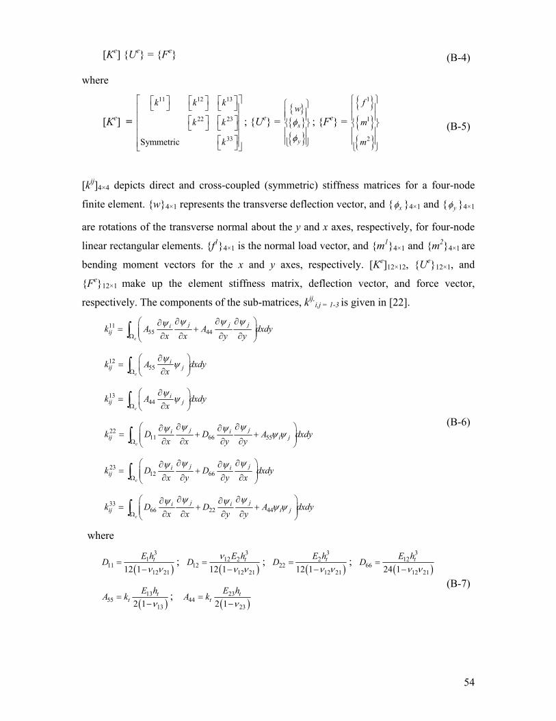
54

[Ke] Ue = Fe (B-4)

where

[Ke] =

11 12 13

22 23

33Symmetric

k k k

k k

k

⎡ ⎤⎡ ⎤ ⎡ ⎤ ⎡ ⎤⎣ ⎦ ⎣ ⎦ ⎣ ⎦⎢ ⎥

⎢ ⎥⎡ ⎤ ⎡ ⎤⎢ ⎥⎣ ⎦ ⎣ ⎦⎢ ⎥

⎡ ⎤⎢ ⎥⎣ ⎦⎣ ⎦

; Ue =

x

y

wφ

φ

⎧ ⎫⎪ ⎪⎪ ⎪⎨ ⎬⎪ ⎪⎪ ⎪⎩ ⎭

; Fe =

1

1

2

f

m

m

⎧ ⎫⎪ ⎪⎪ ⎪⎨ ⎬⎪ ⎪⎪ ⎪⎩ ⎭

(B-5)

[kij]4×4 depicts direct and cross-coupled (symmetric) stiffness matrices for a four-node

finite element. w4×1 represents the transverse deflection vector, and xφ 4×1 and yφ 4×1

are rotations of the transverse normal about the y and x axes, respectively, for four-node

linear rectangular elements. f14×1 is the normal load vector, and m14×1 and m24×1 are

bending moment vectors for the x and y axes, respectively. [Ke]12×12, Ue12×1, and

Fe12×1 make up the element stiffness matrix, deflection vector, and force vector,

respectively. The components of the sub-matrices, kij,i,j = 1-3

is given in [22].

1155 44

e

j j jiijk A A dxdy

x x y yψ ψ ψψ

Ω

∂ ∂ ∂⎛ ⎞∂= +⎜ ⎟⎜ ⎟∂ ∂ ∂ ∂⎝ ⎠∫

1255

e

iij jk A dxdy

xψ

ψΩ

∂⎛ ⎞= ⎜ ⎟∂⎝ ⎠∫

1344

e

iij jk A dxdy

xψ

ψΩ

∂⎛ ⎞= ⎜ ⎟∂⎝ ⎠∫

2211 66 55

e

j ji iij i jk D D A dxdy

x x y yψ ψψ ψ

ψ ψΩ

∂ ∂⎛ ⎞∂ ∂= + +⎜ ⎟⎜ ⎟∂ ∂ ∂ ∂⎝ ⎠∫

2312 66

e

j ji iijk D D dxdy

x y y xψ ψψ ψ

Ω

∂ ∂⎛ ⎞∂ ∂= +⎜ ⎟⎜ ⎟∂ ∂ ∂ ∂⎝ ⎠∫

3366 22 44

e

j ji iij i jk D D A dxdy

x x y yψ ψψ ψ

ψ ψΩ

∂ ∂⎛ ⎞∂ ∂= + +⎜ ⎟⎜ ⎟∂ ∂ ∂ ∂⎝ ⎠∫

(B-6)

where

( )

31

1112 2112 1tE h

Dν ν

=−

; ( )

312 2

1212 2112 1

tE hD

νν ν

=−

; ( )

32

2212 2112 1tE h

Dν ν

=−

; ( )

312

6612 2124 1tE h

Dν ν

=−

( )

1355

132 1t

tE h

A kν

=−

; ( )

2344

232 1t

tE h

A kν

=−

(B-7)