COMPUTATION OF THE CANONICAL …tgkolda/tdw2004/ldl-01-109.pdfcomputation of the canonical...
33
COMPUTATION OF THE CANONICAL DECOMPOSITION BY MEANS OF A SIMULTANEOUS GENERALIZED SCHUR DECOMPOSITION ∗ LIEVEN DE LATHAUWER † , BART DE MOOR ‡ , AND JOOS VANDEWALLE ‡ SIAM J. MATRIX ANAL. APPL. c 2004 Society for Industrial and Applied Mathematics Vol. 26, No. 2, pp. 295–327 Abstract. The canonical decomposition of higher-order tensors is a key tool in multilinear algebra. First we review the state of the art. Then we show that, under certain conditions, the problem can be rephrased as the simultaneous diagonalization, by equivalence or congruence, of a set of matrices. Necessary and sufficient conditions for the uniqueness of these simultaneous matrix decompositions are derived. In a next step, the problem can be translated into a simultaneous generalized Schur decomposition, with orthogonal unknowns [A.-J. van der Veen and A. Paulraj, IEEE Trans. Signal Process., 44 (1996), pp. 1136–1155]. A first-order perturbation analysis of the simultaneous generalized Schur decomposition is carried out. We discuss some computational techniques (including a new Jacobi algorithm) and illustrate their behavior by means of a number of numerical experiments. Key words. multilinear algebra, higher-order tensor, canonical decomposition, parallel factors analysis, generalized Schur decomposition AMS subject classifications. 15A18, 15A69 DOI. 10.1137/S089547980139786X 1. Introduction. An increasing number of signal processing problems involves the manipulation of quantities of which the elements are addressed by more than two indices. In the literature these higher-order equivalents of vectors (first order) and matrices (second order) are called higher-order tensors, multidimensional matri- ces, or multiway arrays. For a lot of applications involving higher-order tensors, the existing framework of vector and matrix algebra appears to be insufficient and/or inappropriate. The algebra of higher-order tensors is called multilinear algebra. Rank-related issues in multilinear algebra are thoroughly different from their ma- trix counterparts. Let us first introduce some definitions. A rank-1 tensor is a tensor that consists of the outer product of a number of vectors. For an N th-order tensor A and N vectors U (1) , U (2) , ..., U (N) , this means that a i1i2...i N = u (1) i1 u (2) i2 ...u (N) i N for all values of the indices, which will be concisely written as A = U (1) ◦ U (2) ◦···◦ U (N) . An n-mode vector of an (I 1 × I 2 ×···× I N )-tensor A is an I n -dimensional vector obtained from A by varying the index i n and keeping the other indices fixed. The n-rank of a higher-order tensor is the obvious generalization of the column (row) rank of matrices: it equals the dimension of the vector space spanned by the n-mode vec- ∗ Received by the editors November 12, 2001; accepted for publication (in revised form) by D. P. O’Leary, November 21, 2003; published electronically November 17, 2004. This research was supported by (1) the Flemish Government: (a) Research Council K.U.Leuven: GOA-MEFISTO- 666, IDO, (b) the Fund for Scientific Research-Flanders (F.W.O.) projects G.0240.99, G.0115.01, G.0197.02, and G.0407.02, (c) the F.W.O. Research Communities ICCoS and ANMMM, (d) project BIL 98 with South Africa; (2) the Belgian State, Prime Minister’s Office, Federal Office for Scientific, Technical and Cultural Affairs, Interuniversity Poles of Attraction Programme IUAP IV-02 and IUAP V-22. http://www.siam.org/journals/simax/26-2/39786.html † ETIS, UMR 8051, 6 avenue du Ponceau, BP 44, F 95014 Cergy-Pontoise Cedex, France ([email protected], http://www.etis.ensea.fr). ‡ SCD-SISTA of the E.E. Dept. (ESAT) of the K.U.Leuven, Kasteelpark Arenberg 10, B-3001 Leu- ven (Heverlee), Belgium ([email protected], [email protected], http://www. esat.kuleuven.ac.be/sista-cosic-docarch/). 295
Transcript of COMPUTATION OF THE CANONICAL …tgkolda/tdw2004/ldl-01-109.pdfcomputation of the canonical...
COMPUTATION OF THE CANONICAL DECOMPOSITION BYMEANS OF A SIMULTANEOUS GENERALIZED SCHUR
DECOMPOSITION∗
LIEVEN DE LATHAUWER† , BART DE MOOR‡ , AND JOOS VANDEWALLE‡
SIAM J. MATRIX ANAL. APPL. c© 2004 Society for Industrial and Applied MathematicsVol. 26, No. 2, pp. 295–327
Abstract. The canonical decomposition of higher-order tensors is a key tool in multilinearalgebra. First we review the state of the art. Then we show that, under certain conditions, theproblem can be rephrased as the simultaneous diagonalization, by equivalence or congruence, of aset of matrices. Necessary and sufficient conditions for the uniqueness of these simultaneous matrixdecompositions are derived. In a next step, the problem can be translated into a simultaneousgeneralized Schur decomposition, with orthogonal unknowns [A.-J. van der Veen and A. Paulraj,IEEE Trans. Signal Process., 44 (1996), pp. 1136–1155]. A first-order perturbation analysis ofthe simultaneous generalized Schur decomposition is carried out. We discuss some computationaltechniques (including a new Jacobi algorithm) and illustrate their behavior by means of a numberof numerical experiments.
Key words. multilinear algebra, higher-order tensor, canonical decomposition, parallel factorsanalysis, generalized Schur decomposition
AMS subject classifications. 15A18, 15A69
DOI. 10.1137/S089547980139786X
1. Introduction. An increasing number of signal processing problems involvesthe manipulation of quantities of which the elements are addressed by more thantwo indices. In the literature these higher-order equivalents of vectors (first order)and matrices (second order) are called higher-order tensors, multidimensional matri-ces, or multiway arrays. For a lot of applications involving higher-order tensors, theexisting framework of vector and matrix algebra appears to be insufficient and/orinappropriate. The algebra of higher-order tensors is called multilinear algebra.
Rank-related issues in multilinear algebra are thoroughly different from their ma-trix counterparts. Let us first introduce some definitions. A rank-1 tensor is a tensorthat consists of the outer product of a number of vectors. For an Nth-order tensor Aand N vectors U (1), U (2), . . . , U (N), this means that ai1i2...iN = u
(1)i1
u(2)i2
. . . u(N)iN
for
all values of the indices, which will be concisely written as A = U (1) U (2) · · · U (N).An n-mode vector of an (I1 × I2 × · · · × IN )-tensor A is an In-dimensional vectorobtained from A by varying the index in and keeping the other indices fixed. Then-rank of a higher-order tensor is the obvious generalization of the column (row) rankof matrices: it equals the dimension of the vector space spanned by the n-mode vec-
∗Received by the editors November 12, 2001; accepted for publication (in revised form) by D.P. O’Leary, November 21, 2003; published electronically November 17, 2004. This research wassupported by (1) the Flemish Government: (a) Research Council K.U.Leuven: GOA-MEFISTO-666, IDO, (b) the Fund for Scientific Research-Flanders (F.W.O.) projects G.0240.99, G.0115.01,G.0197.02, and G.0407.02, (c) the F.W.O. Research Communities ICCoS and ANMMM, (d) projectBIL 98 with South Africa; (2) the Belgian State, Prime Minister’s Office, Federal Office for Scientific,Technical and Cultural Affairs, Interuniversity Poles of Attraction Programme IUAP IV-02 and IUAPV-22.
http://www.siam.org/journals/simax/26-2/39786.html†ETIS, UMR 8051, 6 avenue du Ponceau, BP 44, F 95014 Cergy-Pontoise Cedex, France
([email protected], http://www.etis.ensea.fr).‡SCD-SISTA of the E.E. Dept. (ESAT) of the K.U.Leuven, Kasteelpark Arenberg 10, B-3001 Leu-
ven (Heverlee), Belgium ([email protected], [email protected], http://www.esat.kuleuven.ac.be/sista-cosic-docarch/).
295
296 L. DE LATHAUWER, B. DE MOOR, AND J. VANDEWALLE
tors. An important difference with the rank of matrices is that the different n-ranksof a higher-order tensor are not necessarily the same. The n-rank will be denoted asrankn(A) = Rn. Even when all the n-ranks are the same, they can still be differentfrom the rank of the tensor, denoted as rank(A) = R; A having rank R generallymeans that it can be decomposed in a sum of R, but not less than R, rank-1 terms;see, e.g., [34].
Example 1. Consider the (2 × 2 × 2)-tensor A defined by⎧⎨⎩
a111 = a112 = 1,a221 = a222 = 2,a211 = a121 = a212 = a122 = 0.
The 1-mode vectors are the columns of the matrix(1 0 1 00 2 0 2
).
Because of the symmetry, the set of 2-mode vectors is the same as the set of 1-modevectors. The 3-mode vectors are the columns of the matrix(
1 0 0 21 0 0 2
).
Hence, we have that R1 = R2 = 2 but R3 = 1.Example 2. Consider the (2 × 2 × 2)-tensor A defined by
a211 = a121 = a112 = 1,a111 = a222 = a122 = a212 = a221 = 0.
The 1-rank, 2-rank, and 3-rank are equal to 2. The rank, however, equals 3, since
A = E2 E1 E1 + E1 E2 E1 + E1 E1 E2,
in which
E1 =
(10
), E2 =
(01
)
is a decomposition in a minimal linear combination of rank-1 tensors (a proof is givenin [17]).
The scalar product 〈A,B〉 of two tensors A,B ∈ RI1×I2×...×IN is defined in a
straightforward way as 〈A,B〉 def=
∑i1
∑i2. . .
∑iN
ai1i2...iN bi1i2...iN . The Frobenius-
norm of a tensor A ∈ RI1×I2×...×IN is then defined as ‖A‖ def
=√〈A,A〉. Two tensors
are called orthogonal when their scalar product is zero.In [19] we discussed a possible multilinear generalization of the singular value de-
composition (SVD). The different n-rank values can easily be read from this decom-position. In [20] we examined some techniques to compute the least-squares approx-imation of a given tensor by a tensor with prespecified n-ranks. On the other hand,in [19] we emphasized that the decomposition that was being studied, is not necessar-ily rank-revealing. This is a drawback of unitary (orthogonal) tensor decompositionsin general. In this paper we will study the decomposition of a given tensor as a linearcombination of a minimal number of possibly nonorthogonal, rank-1 terms. This type
A CANDECOMP ALGORITHM 297
of decomposition is often called “canonical decomposition” (CANDECOMP) or “par-allel factors” model (PARAFAC). It is a multilinear generalization of diagonalizing amatrix by an equivalence or congruence transformation. However, it has thoroughlydifferent properties, e.g., as far as uniqueness is concerned.
Section 2 is a brief introduction to the subject, with a formal definition of theCANDECOMP-concept and an overview of the main current computational tech-niques. In this section we will also mark out the problem that we will consider inthis paper (we will make some specific assumptions concerning the linear indepen-dence of the canonical components). In section 3 we discuss a preprocessing step thatallows us to reduce the dimensionality of the problem. In section 4 we establish acomputational link between the tensor decomposition and the simultaneous diagonal-ization of a set of matrices by equivalence or congruence; this problem might also belooked at as a simultaneous matrix eigenvalue decomposition (EVD). The fact thatthe CANDECOMP usually involves nonorthogonal factor matrices is numerically dis-advantageous. By reformulating the problem as a simultaneous generalized Schurdecomposition (SGSD), the unknowns are restricted to the manifold of orthogonalmatrices in section 5. In section 6 we discuss the advantage of working via a simulta-neous matrix decomposition as opposed to working via a single EVD; this section alsocontains a first-order perturbation analysis of the SGSD. Techniques for the actualcomputation of the SGSD are considered in section 7. In section 8 it is explained howthe original CANDECOMP-components can be retrieved from the components of theSGSD. In section 9 the different techniques are illustrated by means of a number ofnumerical experiments.
This paper contains the following new contributions:• In the literature one finds that, in theory, the CANDECOMP can be com-
puted by means of a matrix EVD (under the uniqueness assumptions specifiedin section 2) [38, 43, 5, 42]. We show that one can actually interpret the ten-sor decomposition as a simultaneous matrix decomposition. The simultaneousmatrix decomposition is numerically more robust than a single EVD.
• We show that the CANDECOMP can be reformulated as an orthogonal si-multaneous matrix decomposition—the SGSD. The reformulation in terms oforthogonal unknowns allows for the application of typical numerical proce-dures that involve orthogonal matrices. The SGSD as such already appearedin [48]. The difference is that in this paper it is applied to unsymmetric,instead of symmetric, matrices. This generalization may raise some confu-sion. It might, for instance, be tempting to consider also a simultaneous lowertriangularization, in addition to a simultaneous upper triangularization.
• We derive a Jacobi-algorithm for the computation of the SGSD. The formulafor the determination of the rotation angle is an explicit solution for the caseof rank-2 tensors.
• The way in which the canonical components are derived from the componentsof the SGSD is more general and more robust than the procedure proposedin [48].
• We derive necessary and sufficient conditions for the uniqueness of a numberof simultaneous matrix decompositions: (1) simultaneous diagonalization byequivalence or congruence, (2) simultaneous EVD of nonsymmetric matrices,(3) simultaneous Schur decomposition (SSD).
• We conduct a first-order perturbation analysis of the SGSD.Before starting with the next section, we add a comment on the notation that is
used. To facilitate the distinction between scalars, vectors, matrices and higher-order
298 L. DE LATHAUWER, B. DE MOOR, AND J. VANDEWALLE
tensors, the type of a given quantity will be reflected by its representation: scalarsare denoted by lower-case letters (a, b, . . . ; α, β, . . . ), vectors are written as capitals(A, B, . . . ) (italic shaped), matrices correspond to bold-face capitals (A, B, . . . ) andtensors are written as calligraphic letters (A, B, . . . ). This notation is consistentlyused for lower-order parts of a given structure. For instance, the entry with row indexi and column index j in a matrix A, i.e., (A)ij , is symbolized by aij (also (A)i = aiand (A)i1i2...iN = ai1i2...iN ); furthermore, the ith column vector of a matrix A isdenoted as Ai, i.e., A = [A1A2 . . .]. To enhance the overall readability, we have madeone exception to this rule: as we frequently use the characters i, j, r, and n in themeaning of indices (counters), I, J , R, and N will be reserved to denote the indexupper bounds, unless stated otherwise.
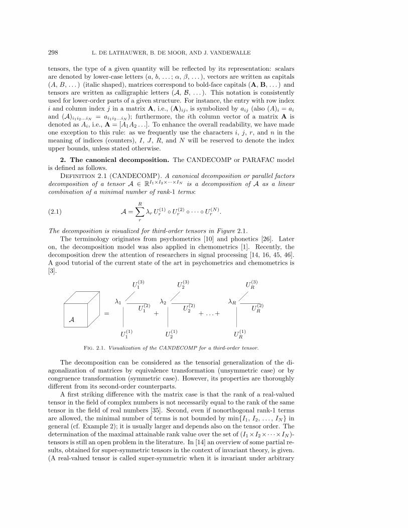
2. The canonical decomposition. The CANDECOMP or PARAFAC modelis defined as follows.
Definition 2.1 (CANDECOMP). A canonical decomposition or parallel factorsdecomposition of a tensor A ∈ R
I1×I2×···×IN is a decomposition of A as a linearcombination of a minimal number of rank-1 terms:
A =
R∑r
λr U(1)r U (2)
r · · · U (N)r .(2.1)
The decomposition is visualized for third-order tensors in Figure 2.1.The terminology originates from psychometrics [10] and phonetics [26]. Later
on, the decomposition model was also applied in chemometrics [1]. Recently, thedecomposition drew the attention of researchers in signal processing [14, 16, 45, 46].A good tutorial of the current state of the art in psychometrics and chemometrics is[3].
A= + . . . ++
U(1)1
λ1 λ2 λR
U(1)2 U
(1)R
U(2)1 U
(2)2 U
(2)R
U(3)1 U
(3)2 U
(3)R
Fig. 2.1. Visualization of the CANDECOMP for a third-order tensor.
The decomposition can be considered as the tensorial generalization of the di-agonalization of matrices by equivalence transformation (unsymmetric case) or bycongruence transformation (symmetric case). However, its properties are thoroughlydifferent from its second-order counterparts.
A first striking difference with the matrix case is that the rank of a real-valuedtensor in the field of complex numbers is not necessarily equal to the rank of the sametensor in the field of real numbers [35]. Second, even if nonorthogonal rank-1 termsare allowed, the minimal number of terms is not bounded by minI1, I2, . . . , IN ingeneral (cf. Example 2); it is usually larger and depends also on the tensor order. Thedetermination of the maximal attainable rank value over the set of (I1×I2×· · ·×IN )-tensors is still an open problem in the literature. In [14] an overview of some partial re-sults, obtained for super-symmetric tensors in the context of invariant theory, is given.(A real-valued tensor is called super-symmetric when it is invariant under arbitrary
A CANDECOMP ALGORITHM 299
index permutations.) The paper includes a tensor-independent rank upper-bound, analgorithm to compute maximal generic ranks and a complete discussion of the case ofsuper-symmetric (2 × 2 × · · · × 2)-tensors.
The uniqueness properties of the CANDECOMP are also very different from (andmuch more complicated than) their matrix equivalents. The theorems of [14] allow oneto determine the dimensionality of the set of valid decompositions for generic super-symmetric tensors. The deepest result concerning uniqueness of the decomposition forthird-order real-valued tensors is derived from a combinatorial algebraic perspectivein [34]. The complex counterpart is concisely proved in [45]. The result is generalizedto arbitrary tensor orders in [47]. In [6] complex fourth-order cumulant tensors areaddressed. Here we will restrict ourselves to some remarks of a more general nature,that are of direct importance to this paper. From the CANDECOMP-definition it isclear that the decomposition is insensitive to
• a permutation of the rank-1 terms,
• a scaling of the vectors U(n)r , combined with the inverse scaling of the coeffi-
cients λr.Apart from these trivial indeterminacies, uniqueness of the CANDECOMP has beenestablished under mild conditions of linear independence (see further for a preciseformulation of the conditions imposed in this paper). Contrarily, the decompositionof a matrix A in a sum of rank(A) rank-1 terms is usually made unique by impos-ing stronger (e.g., orthogonality) constraints. In addition, for an essentially uniqueCANDECOMP the number of terms R can exceed minI1, I2, . . . , IN.
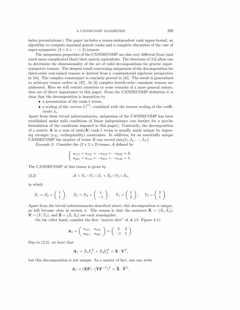
Example 3. Consider the (2 × 2 × 2)-tensor A defined bya111 = a121 = −a212 = −a222 = 3,a221 = a112 = −a211 = −a122 = 1.
The CANDECOMP of this tensor is given by
A = X1 Y1 Z1 + X2 Y2 Z2,(2.2)
in which
X1 = Z2 =
(11
), Z1 = X2 =
(1−1
), Y1 =
(12
), Y2 =
(21
).
Apart from the trivial indeterminacies described above, this decomposition is unique,as will become clear in section 4. The reason is that the matrices X = (X1 X2),Y = (Y1 Y2), and Z = (Z1 Z2) are each nonsingular.
On the other hand, consider the first “matrix slice” of A (cf. Figure 4.1):
A1 =
(a111 a121
a211 a221
)=
(3 3−1 1
).
Due to (2.2), we have that
A1 = X1YT1 + X2Y
T2 = X · YT ,
but this decomposition is not unique. As a matter of fact, one can write
A1 = (XF) · (YF−T )T = X · YT ,
300 L. DE LATHAUWER, B. DE MOOR, AND J. VANDEWALLE
for any nonsingular (2×2) matrix F. One way to make this decomposition essentiallyunique, is to claim that the columns of X and Y are orthogonal. The solution is thengiven by the SVD of A1.
It is a common practice to look for the CANDECOMP-components by straight-forward minimization of the quadratic cost function
f(A) = ‖A − A‖2(2.3)
over all rank-R tensors A, which we will parametrize as
A =
R∑r
λr U(1)r U (2)
r · · · U (N)r .(2.4)
It is possible to resort to an alternating least-squares (ALS) algorithm, in which thevector estimates are updated mode per mode [10]. The idea is as follows. Let usdefine
U(n) def= [U
(n)1 U
(n)2 . . . U
(n)R ],
Λdef= diag(λ1, λ2, . . . , λR),
in which diag· is a diagonal matrix, containing the entries of its argument on the
diagonal. If we now imagine that the matrices U(m), m = n, are fixed, then (2.3) is
merely a quadratic expression in the components of the matrix U(n) · Λ; the estima-tion of these components is a classical linear least-squares problem. An ALS iterationconsists of repeating this procedure for different mode numbers: in each step the esti-mate of one of the matrices U(1),U(2), . . . ,U(N) is optimized, while the other matrixestimates are kept constant. Overflow and underflow can be avoided by normalizing
the estimates of the columns U(n)r (1 r R; 1 n N) to unit-length.
For R = 1, the ALS algorithm can be interpreted as a generalization of the powermethod for the computation of the best rank-1 approximation of a matrix [20]. ForR > 1, however, the canonical components can in principle not be obtained by meansof a deflation algorithm. The reason is that the stationary points of the higher-orderpower iteration generally do not correspond to one of the terms in (2.4), and thatthe residue is in general not of rank R − 1 [32]. This even holds when the rank-1 terms are mutually orthogonal [33]. Only when each of the matrices U(n) iscolumn-wise orthonormal, the deflation approach will work, but in this special case,the components can be obtained by means of a matrix SVD [19].
Because the cost function is monotonically decreasing, one expects that the ALSalgorithm converges to a (local) minimum of f(A). If the CANDECOMP-modelis only approximately valid, the risk of finding a spurious local optimum can bediminished by repeating the optimization for a number of randomly chosen initialvalues. The decision on whether the global optimum has been found or not usuallyrelies on heuristics. The process of iterating over different starting values can betime-consuming. In addition, if the directions of some of the n-mode vectors inthe CANDECOMP-model (1 n N) are close, then it seems unlikely that thisconfiguration is found from a random start [14]. Some alternative initializations arediscussed in [11]. The rank itself is usually determined by repeating the procedurefor different values of R, and comparing the results. An alternative, also based onheuristics, is the evaluation of split-half experiments [27].
A CANDECOMP ALGORITHM 301
ALS iterations can be very slow. In addition, it is sometimes observed that thealgorithm moves through a “swamp”: the algorithm seems to converge, but then theconvergence speed drastically decreases and remains small for several iteration steps,after which it may suddenly increase again. The nature of swamps and how theycan be avoided forms a topic of ongoing research [41, 36]. To cope with the slowconvergence, a number of acceleration methods have been proposed [26, 28, 31]. Onecould make use of a prediction technique, in which estimates of previous iterationsteps are extrapolated to forecast new estimates [3].
In [40] a Gauss–Newton method is described, in which all the CANDECOMP-factors are updated simultaneously; in addition, the inherent indeterminacy of thedecomposition has been fixed by adding a quadratic regularization constraint on thecomponent entries.
On the other hand, setting the gradient of f to zero and solving the resultingset of equations, is computationally hard as well: a set of R(I1 + I2 + . . . IN ) −R(N − 1) polynomial equations of degree 2N − 1, in R(I1 + I2 + . . . IN ) −R(N − 1)independent unknowns, has to be solved (to determine this dimensionality, imaginethat the indeterminacy has been overcome by incorporating the factor λr (1 r R)in one of the vectors of the rth outer product, and by fixing one nonzero entry in theother vectors).
An interesting alternative procedure, which works under a number of assumptionsamong which the most restrictive is that R minI1, I2, has been proposed in [38].Similar results have been proposed in [43, 5, 42]. It was explained that, if (2.1) isexactly valid, the decomposition can be found by a simple matrix EVD. When A isonly known with limited accuracy, a least-squares matching of both sides of (2.1) cannow be initialized with the EVD result. This technique forms the starting point forthe developments in section 4.
Some promising computation schemes, at this moment only formulated in termsof (super-symmetric) cumulant tensors, have been developed as means to solve theproblem of higher-order-only independent component analysis. In [7] Cardoso showsthat under mild conditions the matrices in the intersection of the range of the cumulanttensor and the manifold of rank-1 matrices take the form of an outer product of asteering vector with itself; consequently MUSIC-like [44] algorithms are devised. In [6]the same author investigates the link between symmetry of the cumulant tensor andthe rank-1 property of its components. The problem is subsequently reformulated interms of a matrix EVD.
The decomposition of a dataset as a sum of rank-1 terms is sometimes calledthe factor analysis problem. With the decomposition, one aims at relating the dif-ferent rank-1 terms to the different “physical mechanisms” that have contributed tothe dataset. We repeat that factor analysis of matrices is, as such, essentially un-derdetermined. The extra conditions (maximal variance, orthonormality, etc.) thatare usually imposed to guarantee uniqueness, are often physically irrelevant. In awide range of parameters, this is not the case for the higher-order decomposition; theweaker conditions of linear independence to ensure uniqueness often have a physicalmeaning. This makes the CANDECOMP of higher-order tensors to an importantsignal processing tool.
In this paper, we will study the special but important case of an (I1 × I2 × I3)-tensor A with rank R minI1, I2 and 3-rank R3 2. (If R3 = 1, then thedifferent matrices obtained from A by fixing the index i3 are proportional, and theCANDECOMP reduces to the diagonalization of one of these matrices by congruence
302 L. DE LATHAUWER, B. DE MOOR, AND J. VANDEWALLE
or equivalence.) We assume that
(i) the set U (1)r (1rR) is linearly independent (i.e., no vector can be written
as a linear combination of the other vectors),
(ii) the set U (2)r (1rR) is linearly independent,
(iii) the set U (3)r (1rR) does not contain collinear vectors (i.e., no vector is a
scalar multiple of an other vector).
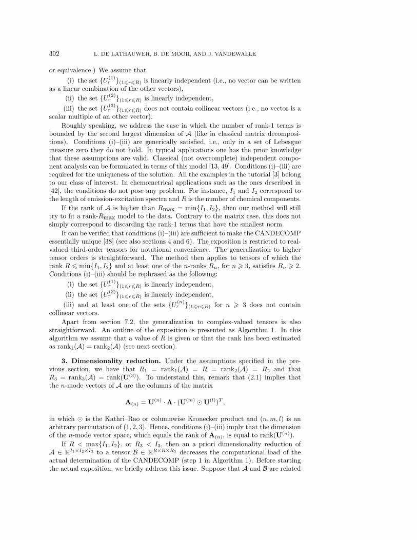
Roughly speaking, we address the case in which the number of rank-1 terms isbounded by the second largest dimension of A (like in classical matrix decomposi-tions). Conditions (i)–(iii) are generically satisfied, i.e., only in a set of Lebesguemeasure zero they do not hold. In typical applications one has the prior knowledgethat these assumptions are valid. Classical (not overcomplete) independent compo-nent analysis can be formulated in terms of this model [13, 49]. Conditions (i)–(iii) arerequired for the uniqueness of the solution. All the examples in the tutorial [3] belongto our class of interest. In chemometrical applications such as the ones described in[42], the conditions do not pose any problem. For instance, I1 and I2 correspond tothe length of emission-excitation spectra and R is the number of chemical components.
If the rank of A is higher than Rmax = minI1, I2, then our method will stilltry to fit a rank-Rmax model to the data. Contrary to the matrix case, this does notsimply correspond to discarding the rank-1 terms that have the smallest norm.
It can be verified that conditions (i)–(iii) are sufficient to make the CANDECOMPessentially unique [38] (see also sections 4 and 6). The exposition is restricted to real-valued third-order tensors for notational convenience. The generalization to highertensor orders is straightforward. The method then applies to tensors of which therank R minI1, I2 and at least one of the n-ranks Rn, for n 3, satisfies Rn 2.Conditions (i)–(iii) should be rephrased as the following:
(i) the set U (1)r (1rR) is linearly independent,
(ii) the set U (2)r (1rR) is linearly independent,
(iii) and at least one of the sets U (n)r (1rR) for n 3 does not contain
collinear vectors.
Apart from section 7.2, the generalization to complex-valued tensors is alsostraightforward. An outline of the exposition is presented as Algorithm 1. In thisalgorithm we assume that a value of R is given or that the rank has been estimatedas rank1(A) = rank2(A) (see next section).
3. Dimensionality reduction. Under the assumptions specified in the pre-vious section, we have that R1 = rank1(A) = R = rank2(A) = R2 and thatR3 = rank3(A) = rank(U(3)). To understand this, remark that (2.1) implies thatthe n-mode vectors of A are the columns of the matrix
A(n) = U(n) · Λ · (U(m) U(l))T ,
in which is the Kathri–Rao or columnwise Kronecker product and (n,m, l) is anarbitrary permutation of (1, 2, 3). Hence, conditions (i)–(iii) imply that the dimensionof the n-mode vector space, which equals the rank of A(n), is equal to rank(U(n)).
If R < maxI1, I2, or R3 < I3, then an a priori dimensionality reduction ofA ∈ R
I1×I2×I3 to a tensor B ∈ RR×R×R3 decreases the computational load of the
actual determination of the CANDECOMP (step 1 in Algorithm 1). Before startingthe actual exposition, we briefly address this issue. Suppose that A and B are related
A CANDECOMP ALGORITHM 303
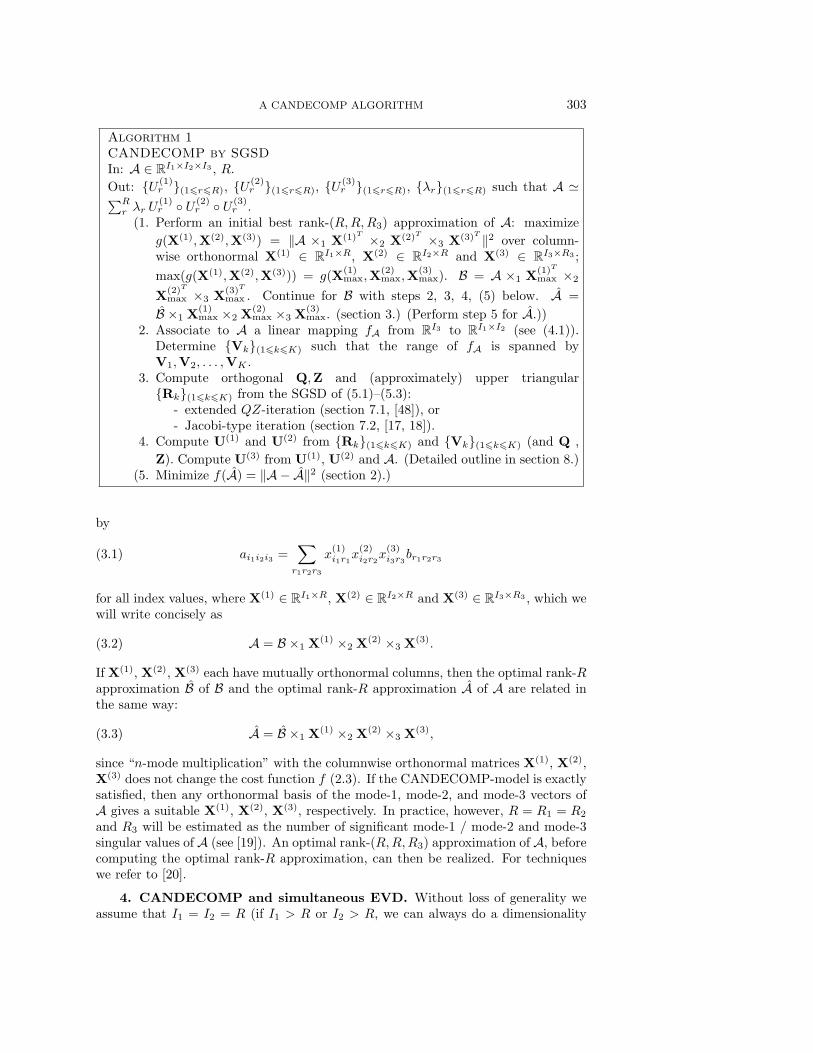
Algorithm 1
CANDECOMP by SGSD
In: A ∈ RI1×I2×I3 , R.
Out: U (1)r (1rR), U (2)
r (1rR), U (3)r (1rR), λr(1rR) such that A ∑R
r λr U(1)r U (2)
r U (3)r .
(1. Perform an initial best rank-(R,R,R3) approximation of A: maximize
g(X(1),X(2),X(3)) = ‖A ×1 X(1)T ×2 X(2)T ×3 X(3)T ‖2 over column-wise orthonormal X(1) ∈ R
I1×R, X(2) ∈ RI2×R and X(3) ∈ R
I3×R3 ;
max(g(X(1),X(2),X(3))) = g(X(1)max,X
(2)max,X
(3)max). B = A ×1 X
(1)T
max ×2
X(2)T
max ×3 X(3)T
max . Continue for B with steps 2, 3, 4, (5) below. A =
B ×1 X(1)max ×2 X
(2)max ×3 X
(3)max. (section 3.) (Perform step 5 for A.))
2. Associate to A a linear mapping fA from RI3 to R
I1×I2 (see (4.1)).Determine Vk(1kK) such that the range of fA is spanned byV1,V2, . . . ,VK .
3. Compute orthogonal Q,Z and (approximately) upper triangularRk(1kK) from the SGSD of (5.1)–(5.3):
- extended QZ-iteration (section 7.1, [48]), or- Jacobi-type iteration (section 7.2, [17, 18]).
4. Compute U(1) and U(2) from Rk(1kK) and Vk(1kK) (and Q ,
Z). Compute U(3) from U(1), U(2) and A. (Detailed outline in section 8.)(5. Minimize f(A) = ‖A − A‖2 (section 2).)
by
ai1i2i3 =∑
r1r2r3
x(1)i1r1
x(2)i2r2
x(3)i3r3
br1r2r3(3.1)
for all index values, where X(1) ∈ RI1×R, X(2) ∈ R
I2×R and X(3) ∈ RI3×R3 , which we
will write concisely as
A = B ×1 X(1) ×2 X(2) ×3 X(3).(3.2)
If X(1), X(2), X(3) each have mutually orthonormal columns, then the optimal rank-Rapproximation B of B and the optimal rank-R approximation A of A are related inthe same way:
A = B ×1 X(1) ×2 X(2) ×3 X(3),(3.3)
since “n-mode multiplication” with the columnwise orthonormal matrices X(1), X(2),X(3) does not change the cost function f (2.3). If the CANDECOMP-model is exactlysatisfied, then any orthonormal basis of the mode-1, mode-2, and mode-3 vectors ofA gives a suitable X(1), X(2), X(3), respectively. In practice, however, R = R1 = R2
and R3 will be estimated as the number of significant mode-1 / mode-2 and mode-3singular values of A (see [19]). An optimal rank-(R,R,R3) approximation of A, beforecomputing the optimal rank-R approximation, can then be realized. For techniqueswe refer to [20].
4. CANDECOMP and simultaneous EVD. Without loss of generality weassume that I1 = I2 = R (if I1 > R or I2 > R, we can always do a dimensionality
304 L. DE LATHAUWER, B. DE MOOR, AND J. VANDEWALLE
reduction, as explained in the previous section). We start the derivation of our com-putation scheme with associating to A a linear transformation of the vector space R
I3
to the matrix space RI1×I2 , in the following way:
V = fA(W ) = A×3 W ⇐⇒ vi1i2 =∑i3
ai1i2i3wi3 ,(4.1)
for all index values. Substitution of (4.1) in (2.1) shows that the image of W caneasily be expressed in terms of the CANDECOMP-components:
V = U(1) · D · U(2)T ,(4.2)
in which we have used the following notations:
U(n) def= [U
(n)1 U
(n)2 . . . U
(n)In
],(4.3)
Ddef= diag(λ1, λ2, . . . , λR) · diagU(3)TW.(4.4)
Any matrix in the range of the mapping fA can be diagonalized by equivalence withthe matrices U(1) and U(2). (If A does not change under permutation of its first twoindices, then any matrix in the range can be diagonalized by congruence with thematrix U(1) = U(2).) If the range is spanned by the matrices V1, V2, . . . , VK , thenwe should solve the following simultaneous decomposition:
V1 = U(1) · D1 · U(2)T ,(4.5)
V2 = U(1) · D2 · U(2)T ,(4.6)
...
VK = U(1) · DK · U(2)T ,(4.7)
in which D1,D2, . . . ,DK are diagonal. A possible choice of Vk(1kK) consists ofthe “matrix slices” Ai(1iI3), obtained by fixing the index i3 to i (see Figure 4.1);the corresponding vectors Wi(1iI3) are the canonical unit vectors. An otherpossible choice consists of the K dominant left singular matrices of the mapping in(4.1). In both cases, the cost function
f(U(1), U(2), Dk) =∑k
‖Vk − U(1) · Dk · U(2)T ‖2
corresponds to the CANDECOMP cost function (2.3). The latter choice follows nat-urally from the analysis in section 3 [20].
For later use, we define
U(3) =
⎛⎜⎜⎜⎝
(D1)11 (D1)22 . . . (D1)RR
(D2)11 (D2)22 . . . (D2)RR
......
...(DK)11 (DK)22 . . . (DK)RR
⎞⎟⎟⎟⎠(4.8)
= [W1W2 . . .WK ]T · U(3) · diag(λ1, λ2, . . . , λR).(4.9)
If the CANDECOMP-model is exactly satisfied, then its terms can be computedfrom two of the equations in (4.5)–(4.7). Let us assume that the matrix V1 has
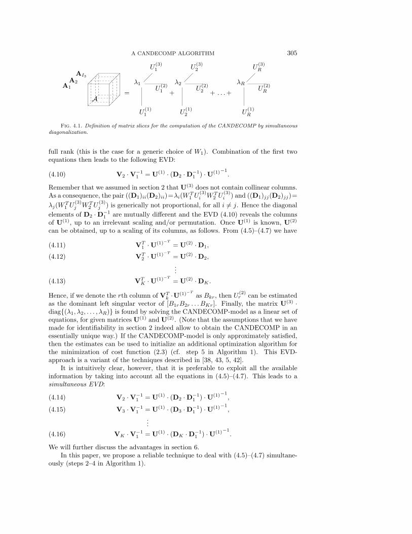
A CANDECOMP ALGORITHM 305
A
A1
A2
AI3
= + . . . ++
U(1)1
λ1 λ2 λR
U(1)2 U
(1)R
U(2)1 U
(2)2 U
(2)R
U(3)1 U
(3)2 U
(3)R
Fig. 4.1. Definition of matrix slices for the computation of the CANDECOMP by simultaneousdiagonalization.
full rank (this is the case for a generic choice of W1). Combination of the first twoequations then leads to the following EVD:
V2 · V−11 = U(1) · (D2 · D−1
1 ) · U(1)−1.(4.10)
Remember that we assumed in section 2 that U(3) does not contain collinear columns.As a consequence, the pair ((D1)ii(D2)ii)=λi(W
T1 U
(3)i WT
2 U(3)i ) and ((D1)jj(D2)jj)=
λj(WT1 U
(3)j WT
2 U(3)j ) is generically not proportional, for all i = j. Hence the diagonal
elements of D2 ·D−11 are mutually different and the EVD (4.10) reveals the columns
of U(1), up to an irrelevant scaling and/or permutation. Once U(1) is known, U(2)
can be obtained, up to a scaling of its columns, as follows. From (4.5)–(4.7) we have
VT1 · U(1)−T
= U(2) · D1,(4.11)
VT2 · U(1)−T
= U(2) · D2,(4.12)
...
VTK · U(1)−T
= U(2) · DK .(4.13)
Hence, if we denote the rth column of VTk ·U(1)−T
as Bkr, then U(2)r can be estimated
as the dominant left singular vector of [B1rB2r . . . BKr]. Finally, the matrix U(3) ·diag(λ1, λ2, . . . , λR) is found by solving the CANDECOMP-model as a linear set ofequations, for given matrices U(1) and U(2). (Note that the assumptions that we havemade for identifiability in section 2 indeed allow to obtain the CANDECOMP in anessentially unique way.) If the CANDECOMP-model is only approximately satisfied,then the estimates can be used to initialize an additional optimization algorithm forthe minimization of cost function (2.3) (cf. step 5 in Algorithm 1). This EVD-approach is a variant of the techniques described in [38, 43, 5, 42].
It is intuitively clear, however, that it is preferable to exploit all the availableinformation by taking into account all the equations in (4.5)–(4.7). This leads to asimultaneous EVD:
V2 · V−11 = U(1) · (D2 · D−1
1 ) · U(1)−1,(4.14)
V3 · V−11 = U(1) · (D3 · D−1
1 ) · U(1)−1,(4.15)
...
VK · V−11 = U(1) · (DK · D−1
1 ) · U(1)−1.(4.16)
We will further discuss the advantages in section 6.In this paper, we propose a reliable technique to deal with (4.5)–(4.7) simultane-
ously (steps 2–4 in Algorithm 1).
306 L. DE LATHAUWER, B. DE MOOR, AND J. VANDEWALLE
5. CANDECOMP and SGSD. The fact that the unknown matrices U(1) andU(2) are basically arbitrary nonsingular matrices, makes them hard to deal with ina proper numerical way. In this section, we will reformulate the problem in termsof orthogonal unknowns. Therefore, we can make an appeal to the technique estab-lished in [48], where the symmetric equivalent of (4.5)–(4.7) was encountered in thederivation of an analytical constant modulus algorithm.
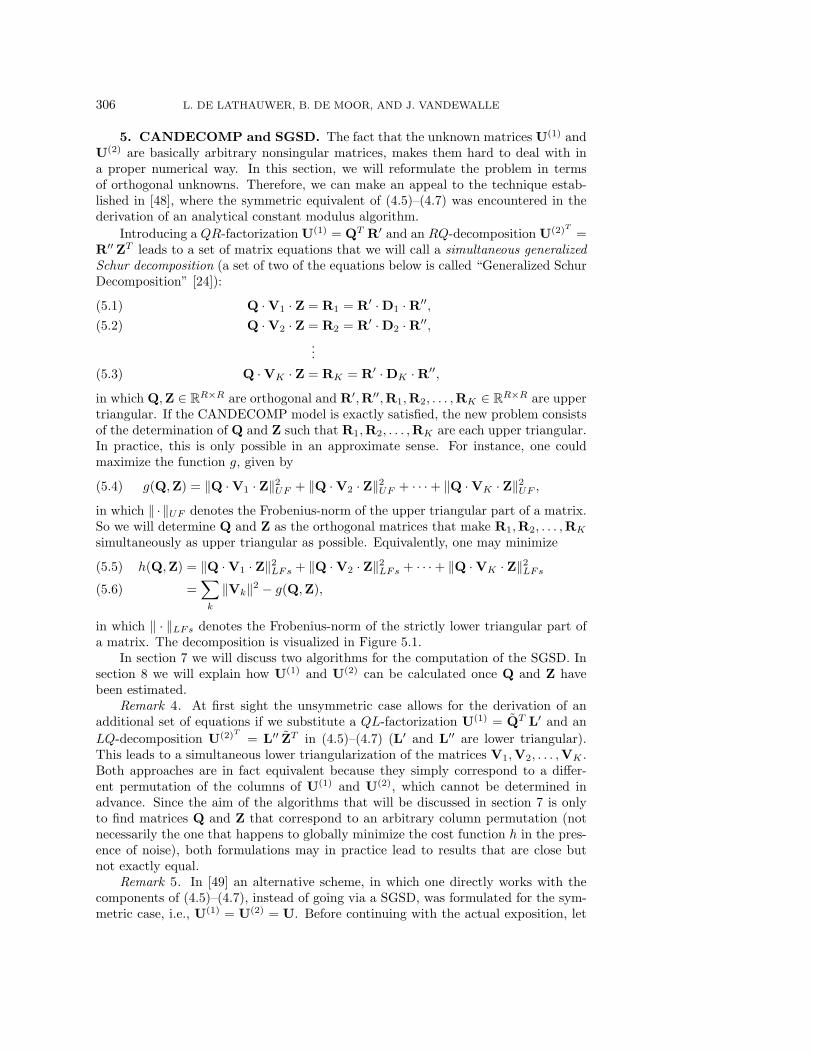
Introducing a QR-factorization U(1) = QT R′ and an RQ-decomposition U(2)T =R′′ ZT leads to a set of matrix equations that we will call a simultaneous generalizedSchur decomposition (a set of two of the equations below is called “Generalized SchurDecomposition” [24]):
Q · V1 · Z = R1 = R′ · D1 · R′′,(5.1)
Q · V2 · Z = R2 = R′ · D2 · R′′,(5.2)
...
Q · VK · Z = RK = R′ · DK · R′′,(5.3)
in which Q,Z ∈ RR×R are orthogonal and R′,R′′,R1,R2, . . . ,RK ∈ R
R×R are uppertriangular. If the CANDECOMP model is exactly satisfied, the new problem consistsof the determination of Q and Z such that R1,R2, . . . ,RK are each upper triangular.In practice, this is only possible in an approximate sense. For instance, one couldmaximize the function g, given by
g(Q,Z) = ‖Q · V1 · Z‖2UF + ‖Q · V2 · Z‖2
UF + · · · + ‖Q · VK · Z‖2UF ,(5.4)
in which ‖ · ‖UF denotes the Frobenius-norm of the upper triangular part of a matrix.So we will determine Q and Z as the orthogonal matrices that make R1,R2, . . . ,RK
simultaneously as upper triangular as possible. Equivalently, one may minimize
h(Q,Z) = ‖Q · V1 · Z‖2LFs + ‖Q · V2 · Z‖2
LFs + · · · + ‖Q · VK · Z‖2LFs(5.5)
=∑k
‖Vk‖2 − g(Q,Z),(5.6)
in which ‖ · ‖LFs denotes the Frobenius-norm of the strictly lower triangular part ofa matrix. The decomposition is visualized in Figure 5.1.
In section 7 we will discuss two algorithms for the computation of the SGSD. Insection 8 we will explain how U(1) and U(2) can be calculated once Q and Z havebeen estimated.
Remark 4. At first sight the unsymmetric case allows for the derivation of anadditional set of equations if we substitute a QL-factorization U(1) = QT L′ and an
LQ-decomposition U(2)T = L′′ ZT in (4.5)–(4.7) (L′ and L′′ are lower triangular).This leads to a simultaneous lower triangularization of the matrices V1,V2, . . . ,VK .Both approaches are in fact equivalent because they simply correspond to a differ-ent permutation of the columns of U(1) and U(2), which cannot be determined inadvance. Since the aim of the algorithms that will be discussed in section 7 is onlyto find matrices Q and Z that correspond to an arbitrary column permutation (notnecessarily the one that happens to globally minimize the cost function h in the pres-ence of noise), both formulations may in practice lead to results that are close butnot exactly equal.
Remark 5. In [49] an alternative scheme, in which one directly works with thecomponents of (4.5)–(4.7), instead of going via a SGSD, was formulated for the sym-metric case, i.e., U(1) = U(2) = U. Before continuing with the actual exposition, let
A CANDECOMP ALGORITHM 307
...
VK
V1
=
=
=
Q
Q
Q
Z
Z
Z
V2
Fig. 5.1. Visualization of a SGSD.
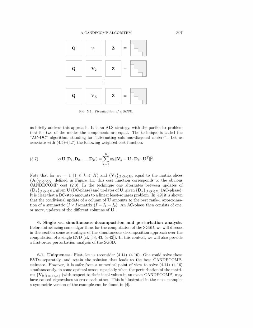
us briefly address this approach. It is an ALS strategy, with the particular problemthat for two of the modes the components are equal. The technique is called the“AC–DC” algorithm, standing for “alternating columns–diagonal centers”. Let usassociate with (4.5)–(4.7) the following weighted cost function:
c(U,D1,D2, . . . ,DK) =
K∑k=1
wk‖Vk − U · Dk · UT ‖2.(5.7)
Note that for wk = 1 (1 k K) and Vk(1kK) equal to the matrix slicesAi(1iI3) defined in Figure 4.1, this cost function corresponds to the obviousCANDECOMP cost (2.3). In the technique one alternates between updates ofDk(1kK), given U (DC-phase) and updates of U, given Dk(1kK) (AC-phase).It is clear that a DC-step amounts to a linear least-squares problem. In [49] it is shownthat the conditional update of a column of U amounts to the best rank-1 approxima-tion of a symmetric (I × I)-matrix (I = I1 = I2). An AC-phase then consists of one,or more, updates of the different columns of U.
6. Single vs. simultaneous decomposition and perturbation analysis.Before introducing some algorithms for the computation of the SGSD, we will discussin this section some advantages of the simultaneous decomposition approach over thecomputation of a single EVD (cf. [38, 43, 5, 42]). In this context, we will also providea first-order perturbation analysis of the SGSD.
6.1. Uniqueness. First, let us reconsider (4.14)–(4.16). One could solve theseEVDs separately, and retain the solution that leads to the best CANDECOMP-estimate. However, it is safer from a numerical point of view to solve (4.14)–(4.16)simultaneously, in some optimal sense, especially when the perturbation of the matri-ces Vk(1kK) (with respect to their ideal values in an exact CANDECOMP) mayhave caused eigenvalues to cross each other. This is illustrated in the next example;a symmetric version of the example can be found in [4].
308 L. DE LATHAUWER, B. DE MOOR, AND J. VANDEWALLE
Example 6. Consider the following matrix pair:
M1 =
⎛⎜⎜⎝
1 − ε 0 0 00 1 + ε 0 00 0 2 10 0 0 3
⎞⎟⎟⎠ , M2 =
⎛⎜⎜⎝
2 1 0 00 3 0 00 0 1 − ε 00 0 0 1 + ε
⎞⎟⎟⎠ ,
in which ε ∈ R is small. For ε = 0, the two matrices have a common eigenmatrix:
E =
⎛⎜⎜⎝
1 1 0 00 1 0 00 0 1 10 0 0 1
⎞⎟⎟⎠ .
If ε = 0, E still nearly diagonalizes V1 and V2:
M1 · E = E · diag[1 1 2 3] + O(ε), M2 · E = E · diag[2 3 1 1] + O(ε).
On the other hand, for ε = 0, the distinct eigenmatrices E1 and E2, of V1 and V2,respectively, are not suitable for diagonalization of the other matrix:
M1 · E2 = E2 · diag[1 1 2 3] + O(1), M2 · E1 = E1 · diag[2 3 1 1] + O(1).
For a simultaneous EVD we have the following uniqueness theorem.Theorem 6.1. For given matrices M1, M2, . . . , ML ∈ R
R×R, the simultaneousdecomposition
M1 = U · D1 · U−1,(6.1)
M2 = U · D2 · U−1,(6.2)
...
ML = U · DL · U−1,(6.3)
with U ∈ RR×R nonsingular and D1, D2, . . . , DL ∈ R
R×R diagonal, is unique up toa permutation and a scaling of the columns of U if and only if all the columns of thematrix
D =
⎛⎜⎜⎜⎝
(D1)11 (D1)22 . . . (D1)RR
(D2)11 (D2)22 . . . (D2)RR
...(DL)11 (DL)22 . . . (DL)RR
⎞⎟⎟⎟⎠
are distinct.Proof. Consider Y = DT ·X, for X ∈ R
L. The ith and jth entry of Y are distinctif X is not perpendicular to Di −Dj . Because Di = Dj , the kernel of DT
i −DTj is a
subspace of dimension L − 1. Let K be the union of the kernels for all i = j and letX ∈ R
L \ K. The EVD of∑
l xlMl is given by
∑l
xlMl = U ·(∑
l
xlDl
)· U−1 = U · diagDT · X · U−1.
Because all eigenvalues are distinct, the eigenmatrix U is unique up to a permutationand a scaling of its columns. On the other hand, if columns of D are equal, it
A CANDECOMP ALGORITHM 309
is not possible to discriminate between different eigenvectors in the correspondingeigenspace.
The equivalent for unitary diagonalization is given in [2].
Because of the link between (4.5)–(4.7) and (4.14)–(4.16), the CANDECOMP isessentially unique when U(1) and U(2) are nonsingular and U(3) does not containcollinear columns, as put forward in section 2.
Theorem 6.1 shows that a simultaneous EVD is much more robust than a singleEVD. It is well known that, when eigenvalues are close, the eigenvectors in a singleEVD may be strongly affected by small perturbations [30]. The reason is that for co-inciding eigenvalues only the corresponding eigenspace is defined; different directionsin this subspace will emerge as eigenvectors for different infinitesimal perturbations.When this happens for one or more of the matrices in a simultaneous EVD, the othermatrices may still allow to identify the actual eigenvectors. We may conclude that,under the conditions of section 2, the CANDECOMP is likely to be stable.
Different permutations of the canonical components will correspond to entirelydifferent matrices Q and Z in the SGSD (5.1)–(5.3). However, these in turn lead todifferent matrices R and R′′ such that, eventually, U(1) and U(2) are still subjectto the same indeterminacies. In other words, the uniqueness condition has not beenweakened by formulating the problem in terms of orthogonal unknowns Q, Z.
It is worth mentioning that, for arbitrary matrices V1, V2, . . . , VK (not satisfyingour CANDECOMP model), the uniqueness conditions of a S(G)SD are much moresevere. In general, only one sequence of (generalized) Schur vectors is possible. Forconvenience, we will illustrate this only for the SSD (which, in our application, wouldarise from substitution of the QR-factorization of U(1) in (4.14)–(4.16)). We have thefollowing theorem.
Theorem 6.2. Let the matrices M1, M2, . . . , ML ∈ RR×R satisfy the SSD
M1 = Q · R1 · QT ,(6.4)
M2 = Q · R2 · QT ,(6.5)
...
ML = Q · RL · QT ,(6.6)
with Q = [Q1Q2 . . . QR] ∈ RR×R orthogonal and R1, R2, . . . , RL ∈ R
R×R uppertriangular. An equivalent simultaneous decomposition, in terms of Q and Rl1lL,
in which the diagonal of (Rl) subsequently contains (Rl)11, (Rl)22, . . . , (Rl)I−1,I−1,(Rl)JJ , (Rl)I+1,I+1, . . . ,(Rl)J−1,J−1, (Rl)II , (Rl)J+1,J+1, . . . , (Rl)KK (1 l L),exists if and only if the following matrix is rank deficient:⎛
⎜⎜⎜⎝M1 − (R1)JJ I [Q1 . . . QI−1] 0 · · · 0M2 − (R2)JJ I 0 [Q1 . . . QI−1] · · · 0
......
.... . .
...ML − (RL)JJ I 0 0 · · · [Q1 . . . QI−1]
⎞⎟⎟⎟⎠ .(6.7)
Proof. Let us first answer the simple question of which diagonal entry could bepermuted to position (1, 1). There is a common eigenvector, other than Q1, if andonly if there exists a J > 1 such that all the equations
(Ml − (Rl)JJ I)X = 0, 1 l L,

310 L. DE LATHAUWER, B. DE MOOR, AND J. VANDEWALLE
have a common solution. This is the condition specified by the theorem for I = 1.One can verify that the upper triangular structure can be maintained for new matricesR1, R2, . . . , RL and Q when the entries at position (J, J) are permuted to position(1, 1) and the old entries at positions (1, 1), (2, 2), . . . , (J − 1, J − 1) are shifted oneplace down on the diagonal. (The strictly upper diagonal entries of rows 1 to J haveto be recomputed.)
In general, the entries at position (J, J) can be brought in Ith position if and onlyif there exists a vector X = 0 and scalars bli, 1 l L, 1 i I − 1, such that
(Ml − (Rl)JJ I)X =
I−1∑i=1
bli Qi, 1 l L.
This is a set of homogeneous linear equations of which the unknowns are the coeffi-cients of X and the scalars bli. The coefficient matrix is given by (6.7).
Moreover, for noisy data, different permutations of the canonical components willlead to matrices Q, Z that yield different values of the cost function h defined in (5.6).
6.2. First-order perturbation analysis. To increase our understanding of thestability of the SGSD, let us now conduct a first-order perturbation analysis.
Theorem 6.3. Consider the function g(Q,Z) in (5.4) and let the matricesR1,R2, . . . ,RK be defined by (5.1)–(5.3). The gradients of g, with respect to Q andZ, over the manifold of orthogonal matrices, are given by
∇Qg = 2 skew
(∑k
upp(Rk)RTk
)· Q,(6.8)
∇Zg = 2Z · skew
(∑k
RTk upp(Rk)
),(6.9)
in which skew(·) is the skew-symmetric and upp(·) the upper triangular part of amatrix.
Proof. We will prove this result by resorting to the framework established in[15, 22]. The gradient of g with respect to Q can be determined by assuming that Qhas a velocity Q on the manifold of orthogonal matrices and expressing the evolutionof g:
g = 〈∇Q g, Q〉(6.10)
(see, e.g., [15, p. 48]; the formula corresponds to a chain rule for the derivation).First we express the function g as
g(Q,Z) =K∑
k=1
〈Q · Vk · Z,upp(Q · Vk · Z)〉.
Assuming that Q is time dependent, the derivative with respect to the time coordinateis given by (taking into account that upp(·) is a linear operation)
g =
K∑k=1
[〈Q · Vk · Z,upp(Q · Vk · Z)〉 + 〈Q · Vk · Z,upp(Q · Vk · Z)〉]
= 2
K∑k=1
〈Q · Vk · Z,upp(Q · Vk · Z)〉.
A CANDECOMP ALGORITHM 311
With a property of the scalar product, we obtain
g = 2
K∑k=1
〈Q,upp(Q · Vk · Z) · ZT · VTk 〉.
The right term is proportional to the gradient of g over RR×R. To ensure that Q
stays on the manifold of orthogonal matrices, we claim additionally that
Q = Ω · Q,
in which Ω ∈ RR×R is skew-symmetric [22, p. 307]. Now the inner product can be
written in the form of (6.10):
g = 2
K∑k=1
〈Ω,upp(Q · Vk · Z) · ZT · VTk · QT 〉
=
⟨Ω, 2
K∑k=1
skewupp(Q · Vk · Z) · ZT · VTk · QT
⟩
=
⟨Ω · Q, 2
K∑k=1
skewupp(Q · Vk · Z) · ZT · VTk · QT · Q
⟩,
which proves (6.8). The gradient with respect to Z can be found in an analogousway.
Theorem 6.4. Consider a first-order perturbation of the matrices in the SGSD(5.1)–(5.3): Vk(ε) = Vk(0) + εBk (1 k K). As a first-order approximation, themaximum of g(Q,Z) is then obtained for
Q(ε) = (I + εΛ + o(ε)) · Q(0),
Z(ε) = Z(0) · (I + εΩ + o(ε)),
in which Λ,Ω ∈ RR×R are skew-symmetric matrices that satisfy the following set of
linear equations: ∑k
lows(RkΩ + Ek + ΛRk) · RTk = 0,(6.11)
∑k
RTk · lows(RkΩ + Ek + ΛRk) = 0,(6.12)
where lows(·) is the strictly lower triangular part of a matrix and
Ek = Q(0) · Bk · Z(0), 1 k K.
Proof. Again, we will work in the framework of [15, 22]. Let us start from (5.1)–(5.3). If the matrices Ak have a velocity Ak = Bk, then Q evolves in such a way thatthe identity ∇Qg ≡ 0 holds. Taking the form of the gradient (6.8) into account, weshould have that
skew
(∑k
upp(Rk)RTk
)≡ 0.(6.13)
312 L. DE LATHAUWER, B. DE MOOR, AND J. VANDEWALLE
Taking the derivative with respect to the time coordinate yields
skew
(∑k
upp(Q · Ak · Z + Q · Ak · Z + Q · Ak · Z)RTk
+upp(Rk)(ZT · AT
k · QT + ZT · ATk · QT + ZT · AT
k · QT )
)= 0.
To ensure that Q and Z stay on the manifold of orthogonal matrices, we claim that
Q = Ω · Q,
Z = Z · Λ,
in which Ω,Λ ∈ RR×R are skew-symmetric. If (5.1)–(5.3) are exactly satisfied, then
upp(Rk) = Rk. Substitution of Ek = Q · Bk · Z then yields
skew
(∑k
Rk · Ω · RTk − upp(Rk · Ω) · RT
k + Ek · RTk − upp(Ek) · RT
k
+Λ · Rk · RTk − upp(Λ · Rk) · RT
k
)= 0
or
skew
(∑k
lows(RkΩ + Ek + ΛRk)RTk
)= 0.
We may drop “skew” because its argument is strictly lower triangular. Equation(6.12) is obtained by starting from the identity ∇Zg ≡ 0.
Remark 7. For matrices Ak that do not allow for an exact upper triangularization,the derivation can be taken over provided that upp(Rk) is not simplified to Rk.
Remark 8. Note that the expressions derived in this section may be used todevelop routines for the computation of the SGSD by means of an optimization overthe (product of two) manifold(s) of orthogonal matrices. We refer to [22].
By the summation in (6.11) and (6.12) the perturbation is to some extent “aver-aged” over the different matrices Ak. When components of Q and Z are ill conditionedfor a subset of Ak, this may be compensated by the other matrices.
7. Algorithms for the SGSD.
7.1. Extended QZ-iteration. For the actual computation of the SGSD, an ex-tended QZ-iteration was proposed in [48]. One alternates between updates of Q andZ in such a way that the cost function h in (5.6) is approximately optimized. In eachstep, the estimate of Q (given Z, or vice-versa) is obtained as a product of matricesH1H2 . . .HR−1, that form the equivalent of Householder matrices for the computationof a simple QR-decomposition [24]. For instance, as far as Q is concerned, H1 max-imally reduces (in least-squares sense) the below-diagonal norm of the first columnsof the instantaneous estimates of R1,R2, . . . ,RK . After multiplication with H1, H2
minimizes the below-diagonal norm of the second columns, without further affectingthe first rows, and so on. H1 is determined through an SVD of an (R × K)-matrix(actually only the left singular vector corresponding to the largest singular value, and
A CANDECOMP ALGORITHM 313
its orthogonal complement, have to be computed), the determination of H2 involvesan SVD of an ((R− 1) ×K)-matrix, and so on.
Because of the high computational cost, it makes sense to initialize the algorithmwith matrices Q(0) and Z(0) defined by two of the equations (5.1)–(5.3). If these twojoint decompositions are well conditioned, then Q(0) and Z(0) may be close to theoptimum; if not, then the extended QZ-iteration may involve more work than just afine tuning of a good initialization.
The resulting scheme is observed to find a good estimate of the global optimum ina limited number of steps, if the CANDECOMP-model is exactly satisfied. However,even moderate perturbations can cause the algorithm to end up in good estimates ofthe theoretical matrices Q and Z that do not globally minimize the cost function. Itis also possible that at some point in the iteration (e.g., initially, or after approximateconvergence), the algorithm starts to increase the value of h. The reason for thisbehavior is that the way in which Q and Z are computed does not imply monotonicconvergence in terms of h: for instance, it is possible that the matrix H1 increases theFrobenius-norm of the part of columns 2 to R − 1 below the diagonal. Nevertheless,these aspects do not seem to pose major problems in practice: over several hundredsof simulations, we have only once obtained a meaningless result.
7.2. Jacobi iteration. In [17, 18] we derived a Jacobi-type algorithm for thecomputation of the SGSD. Here, Q and Z are found as a sequence of elementaryJacobi-rotation matrices. In a step (i, j), Q and Z are multiplied by elementaryrotation matrices, affecting rows and columns i and j. These rotation matrices aresuch that they maximize the function g in (5.4). It turns out that the determinationof a Jacobi-rotation pair basically amounts to rooting a polynomial of degree 8. Onesweeps over all the possible pairs (i, j), and then iterates over such sweeps.
The iteration can be initialized with matrices Q(0) and Z(0), obtained from thegeneralized Schur decomposition corresponding to two of the equations in (5.1)–
(5.3) [24]. Assume that at iteration step l + 1, the estimates Q(l), Z(l), and R(l)1 , . . . ,
R(l)K are available. Let Gij ∈ R
R×R represent an elementary Givens rotation matrixthat affects rows i and j, i.e., Gij equals the identity matrix, except for the entries
(Gij)ii = (Gij)jj = cosα,
(Gij)ji = −(Gij)ij = sinα,
in which α is the rotation angle (assume that j > i). An update of Q(l) takesthe form of Q(l+1) = Gij · Q(l). Similarly, an update of Z(l) takes the form of
Z(l+1) = Z(l) ·G′ij
T, where the Givens rotation matrix G′
ij is defined in the same way
as Gij , in terms of an angle β. At the same time R(l)1 ,R
(l)2 , . . . ,R
(l)K are updated as
R(l+1)1 = Gij ·R(l)
1 ·G′ij
T, R
(l+1)2 = Gij ·R(l)
2 ·G′ij
T, . . . , R
(l+1)K = Gij ·RK
(l) ·G′ij
T.
At iteration step l, the maximization of the function g in (5.4) is equivalent tothe minimization of
h(α, β) =
K∑k=1
[(R
(l+1)k )2ji +
j−1∑r=i+1
((R(l+1)k )2ri + (R
(l+1)k )2jr)
](7.1)
(the other entries do not affect the norm of the strictly lower diagonal parts). Thefunction h is given in explicit form by
h(α, β) =
K∑k=1
5∑n=1
hkn(α, β),(7.2)
314 L. DE LATHAUWER, B. DE MOOR, AND J. VANDEWALLE
in which
hk1(α, β) = sin2 α
×[cos2 β (R(l)k )2ii + sin2 β (R
(l)k )2ij − 2 sinβ cosβ (R
(l)k )ii(R
(l)k )ij ],(7.3)
hk2(α, β) = 2 sinα cosα
cos2 β (R(l)k )ii(R
(l)k )ji + sin2 β (R
(l)k )ij(R
(l)k )jj
− sinβ cosβ [(R(l)k )ij(R
(l)k )ji + (R
(l)k )ii(R
(l)k )jj ]
,(7.4)
hk3(α, β) = cos2 α
×[cos2 β (R(l)k )2ji + sin2 β (R
(l)k )2jj − 2 sinβ cosβ (R
(l)k )ji(R
(l)k )jj ],(7.5)
hk4(α, β) = (sin2 α + cos2 α)
×j−1∑
r=i+1
[cos2 β (R(l)k )2ri + sin2 β (R
(l)k )2rj − 2 sinβ cosβ (R
(l)k )ri(R
(l)k )rj ],(7.6)
hk5(α, β) = (sin2 β + cos2 β)
×j−1∑
r=i+1
[cos2 α (R(l)k )2jr + sin2 α (R
(l)k )2ir + 2 sinα cosα (R
(l)k )ir(R
(l)k )jr].(7.7)
Setting the partial derivatives of h, with respect to α and β, equal to zero, leads to aset of biquadratic equations in tanα and tanβ:
b1(β) tan2 α + b2(β) tanα− b1(β) = 0,(7.8)
b3(β) tan2 α + b4(β) tanα + b5(β) = 0,(7.9)
in which bn(β) =∑K
k=1 bkn(β), with
bk1(β) = tan2 β
(R
(l)k )2ij − (R
(l)k )2jj +
j−1∑r=i+1
[(R(l)k )2ir − (R
(l)k )2jr]
+2 tanβ [(R(l)k )ji(R
(l)k )jj − (R
(l)k )ii(R
(l)k )ij ]
+
(R
(l)k )2ii − (R
(l)k )2ji +
j−1∑r=i+1
[(R(l)k )2ir − (R
(l)k )2jr]
,(7.10)
bk2(β) = tan2 β
[(R
(l)k )ij(R
(l)k )jj +
j−1∑r=i+1
(R(l)k )ir(R
(l)k )jr
]
− tanβ [(R(l)k )ij(R
(l)k )ji + (R
(l)k )ii(R
(l)k )jj ]
+
[(R
(l)k )ii(R
(l)k )ji +
j−1∑r=i+1
(R(l)k )ir(R
(l)k )jr
],(7.11)
bk3(β) = (tan2 β − 1)
[(R
(l)k )ii(R
(l)k )ij +
j−1∑r=i+1
(R(l)k )ri(R
(l)k )jr
]
+ tanβ
(R
(l)k )2ij − (R
(l)k )2ii +
j−1∑r=i+1
[(R(l)k )2rj − (R
(l)k )2ri]
,(7.12)
bk4(β) = (tan2 β − 1) [(R(l)k )ij(R
(l)k )ji + (R
(l)k )ii(R
(l)k )jj ]
A CANDECOMP ALGORITHM 315
+2 tanβ [(R(l)k )ij(R
(l)k )jj − (R
(l)k )ii(R
(l)k )ji],(7.13)
bk5(β) = (tan2 β − 1)
[(R
(l)k )ji(R
(l)k )jj +
j−1∑r=i+1
(R(l)k )ri(R
(l)k )rj
]
+ tanβ
(R
(l)k )2jj − (R
(l)k )2ji +
j−1∑r=i+1
[(R(l)k )2rj − (R
(l)k )2ri]
.(7.14)
The global minimum of h(α, β) can be determined by computing the various solutionsof (7.8)–(7.9) and selecting the one corresponding to the smallest value in (7.2).
For the solution of the set of biquadratic equations, let us first consider the specialcase where (7.8) is linear in tanα: b1(β) = 0. The only ways in which a root β0 ofb1 can lead to a solution of (7.8)–(7.9) are (a) tanα = 0 and additionally b5(β0) = 0and (b) α is a solution of (7.9), for β = β0, which additionally satisfies b2(β0) = 0.
Now let us investigate the general case, i.e., b1(β) = 0. Substitution of the squareroots of (7.8) in (7.9) (considered as quadratic expressions in the unknown tanα) thenleads to the following polynomial of degree 8 in tanβ:
b21(β)b23(β) + b21(β)b25(β) − b1(β)b2(β)b4(β)b5(β) + 2b21(β)b3(β)b5(β)
+ b22(β)b3(β)b5(β) − b21(β)b24(β) + b1(β)b2(β)b3(β)b4(β) = 0.(7.15)
For the roots of this polynomial, the corresponding value of tanα that gives a solutionto (7.8)–(7.9), can be found from
(b2(β)b3(β) − b1(β)b4(β)) tanα− b1(β)(b3(β) + b5(β)) = 0.(7.16)
The computational cost is in line with results obtained for other simultaneousmatrix decompositions. A Jacobi-rotation for a simultaneous real symmetric EVDcan be computed by rooting a polynomial of degree 2 [8, 9]. For an SSD (Q = Z),polynomials are of degree 4 [25].
The Jacobi-result is an explicit solution for the CANDECOMP of rank-2 tensors.Apart from this result, a Jacobi-sweep is more expensive than an extended QZ-stepif not minR,K 8.
If the simultaneous equivalence transformation of (4.5)–(4.7) is not exactly sat-isfied, different permutations of the CANDECOMP components may cause the cor-responding orthogonal factors Q and Z to yield values of the function g that aresomewhat different. There is no guarantee that the Jacobi-algorithm will convergeto the solution with that specific column ordering that leads to the global optimum.Apart from the reordering of columns, there is no formal evidence that the two-sidedJacobi-algorithm cannot get stuck in a local optimum; local or global convergence isstill an open problem for the computation of other simultaneous matrix decomposi-tions as well [4, 8, 9, 12, 23, 48]. We have not observed convergence to a local optimumin any of our simulations for the unsymmetric CANDECOMP-problem. For the casewhere U(1) = U(2), a meaningless result has been obtained for one out of hundredsof simulations. In this odd case, the problem could be overcome by reinitializing thealgorithm.
8. Estimation of the canonical components from the components ofthe SGSD. In this section we will explain how the matrices U(1) and U(2) can beestimated, once Q and Z are known. How U(3) may subsequently be estimated wasexplained in section 4. This corresponds to step 4 in Algorithm 1. Computation of
316 L. DE LATHAUWER, B. DE MOOR, AND J. VANDEWALLE
the SGSD is in general only equivalent to least-squares fitting of the CANDECOMP-model if that model is exactly valid. The estimates obtained so far may then be usedto initialize an additional optimization algorithm for the minimization of cost function(2.3), as also mentioned in section 4 (step 5 in Algorithm 1).
In [48] a procedure has been proposed that works under the assumption that thecolumns of U(3) are linearly independent (and sufficiently well conditioned). Hencethis technique can be used only when K R. The solution is obtained via thecomputation of the pseudoinverse of a (K ×R) matrix and the estimation of the bestrank-1 approximation of R (R×R) matrices.
We will derive a new technique that works under the assumptions establishedin section 2. This technique is also computationally less demanding. It essentiallyrequires solving R(R−1)/2 overdetermined sets of K linear equations in 2 unknowns.
We will estimate R′ and R′′ from (5.1)–(5.3) and then combine them with Qand Z to obtain U(1) and U(2). If we assume that the main diagonals of R′ and R′′
contain only entries equal to 1 (we can make this assumption because the columns ofU(1) and U(2) can be determined only up to a scaling factor), then Dk = diagRk(1 k K), in which diag· now denotes the diagonal part of a matrix. The strictlyupper diagonal elements of R′ and R′′ can be estimated by subsequently solving in aleast-squares sense the equations related to the entries of Rk(1kK) at positions(R− 1, R), (R− 2, R− 1), (R− 2, R), . . . , (1, 2), (1, 3), . . . , (1, R) in (5.1)–(5.3) withrespect to the unknowns r′R−1,R and r′′R−1,R, r′R−2,R−1 and r′′R−2,R−1, r′R−2,R, andr′′R−2,R, . . . , r′1,2 and r′′1,2, r
′1,3 and r′′1,3, . . . , r′1,R and r′′1,R, respectively. For instance,
with the entries at position (R− 1, R) corresponds the equation
⎛⎜⎜⎜⎝
(R1)R,R (R1)R−1,R−1
(R2)R,R (R2)R−1,R−1
......
(RK)R,R (RK)R−1,R−1
⎞⎟⎟⎟⎠
(r′R−1,R
r′′R−1,R
)=
⎛⎜⎜⎜⎝
(R1)R−1,R
(R2)R−1,R
...(RK)R−1,R
⎞⎟⎟⎟⎠ .
Note that, according to the third working assumption made in section 2, the columnsof the matrix on the left-hand side of this equation should be linearly independent.
For the computation of U(3), remark that (4.5)–(4.7) correspond to a CANDE-COMP of a tensor V ∈ R
R×R×K , with entries vijk = (Vk)ij , of which the component
matrices are U(1), U(2) and the matrix U(3) defined in (4.8). Let V(R2×K) ∈ RR2×K ,
with entries
(V(R2×K))(i−1)R+j,k = (Vk)ij ,
be a matrix representation of V. (4.5)–(4.7) can be reformulated as
V(R2×K) = (U(1) U(2)) · U(3)T .(8.1)
U(3) can be computed from this (possibly overdetermined) set of linear equations.Finally, U(3) follows from (4.9).
To conclude, let us give an outline of the computation of U(1), U(2), and U(3)
from the results of the SGSD (5.1)–(5.3). This scheme details step 4 in Algorithm 1.
4.1 Computation of R′ and R′′.Set diagR′ = diagR′′ = I.for i = R− 1, R− 2, . . . , 1
A CANDECOMP ALGORITHM 317
for j = i + 1, i + 2, . . . , R
⎛⎜⎜⎜⎝
(R1)jj (R1)ii(R2)jj (R2)ii
......
(RK)jj (RK)ii
⎞⎟⎟⎟⎠
(r′ijr′′ij
)=
⎛⎜⎜⎜⎜⎝
(R1)ij −∑j−1
p=i+1 r′ip (R1)pp r
′′pj
(R2)ij −∑j−1
p=i+1 r′ip (R2)pp r
′′pj
...
(RK)ij −∑j−1
p=i+1 r′ip (RK)pp r
′′pj
⎞⎟⎟⎟⎟⎠
endend
4.2 U(1) = QT · R′. U(2) = Z · (R′′)T .4.3 Compute U(3) from (8.1). Compute U(3), modulo a scaling of its columns,
from (4.9).
9. Numerical experiments. In this section we illustrate the performance of thealgorithms proposed in this paper by means of a number of numerical experiments.These experiments are helpful to understand and evaluate the different methods, giventhat a rigorous mathematical analysis of their convergence properties often proves tobe extremely tough (as is witnessed by the fact that only very few related results areavailable [4, 50]).
In a first series of experiments we will compare the accuracy of both techniquespresented in section 7 and check whether an additional direct optimization of the costfunction f , defined in (2.3), is needed (step 5 in Algorithm 1). We will also show thatthe extended QZ-iteration is not simply based on the minimization of cost functionh, defined in (5.6).
Tensors A ∈ R3×3×3, of which the canonical components will afterwards be esti-
mated, are generated in the following way:
A = A/‖A‖ + σN N/‖N ‖,(9.1)
in which A exactly satisfies the CANDECOMP-model:
A = U(1)1 U (2)
1 U (3)1 + U
(1)2 U (2)
2 U (3)2 + U
(1)3 U (2)
3 U (3)3 .(9.2)
The components in (9.1)–(9.2) are generated as follows. First consider the (3 × 3)-matrices U(1), U(2), and U(3), defined by (4.3). The entries of 3 (3× 3)-matrices arerandomly taken from a uniform distribution on the interval [0, 1). U(2) and U(3) arederived from two of these matrices by replacing their singular values by 3, 2, 1, whilekeeping the singular vectors. U(1) is generated in the same way but three different setsof singular values will be considered: 3, 2, 1; 30, 15, 1; 100, 50, 1. The entries of Nare drawn from a zero-mean unit-variance Gaussian distribution. For each particularchoice of U(1), U(2), U(3), and N , the scalar σN is varied between 1e− 3 and 1.
For each of the sets of singular values of U(1), 50 independent samples of A arerealized; for each of them 7 logarithmically equidistant values of σN are considered.In each Monte Carlo simulation the following algorithms are run: (a) the Jacobi-algorithm, discussed in section 7.2; (b) a least-squares matching of both sides of (2.3),for which the leastsq command of the Optimization Toolbox 1.0 of MATLAB 4.2 hasbeen used, initialized with the result of (a); and (c) the extended QZ-iteration, de-scribed in section 7.1. The algorithm (a) is terminated if a full sweep no longer allowsthe reduction of the cost function h(Q,Z) with at least 0.01%. The same terminationcriterion is used for a Q-step followed by a Z-step in the extended QZ-iteration. For
318 L. DE LATHAUWER, B. DE MOOR, AND J. VANDEWALLE
the least-squares matching (b) a minimal precision of 1e− 5 for the optimal values ofthe cost function f , defined in (2.3), and the corresponding components is presumed;the MATLAB routine maximally performs 2100 iteration steps.
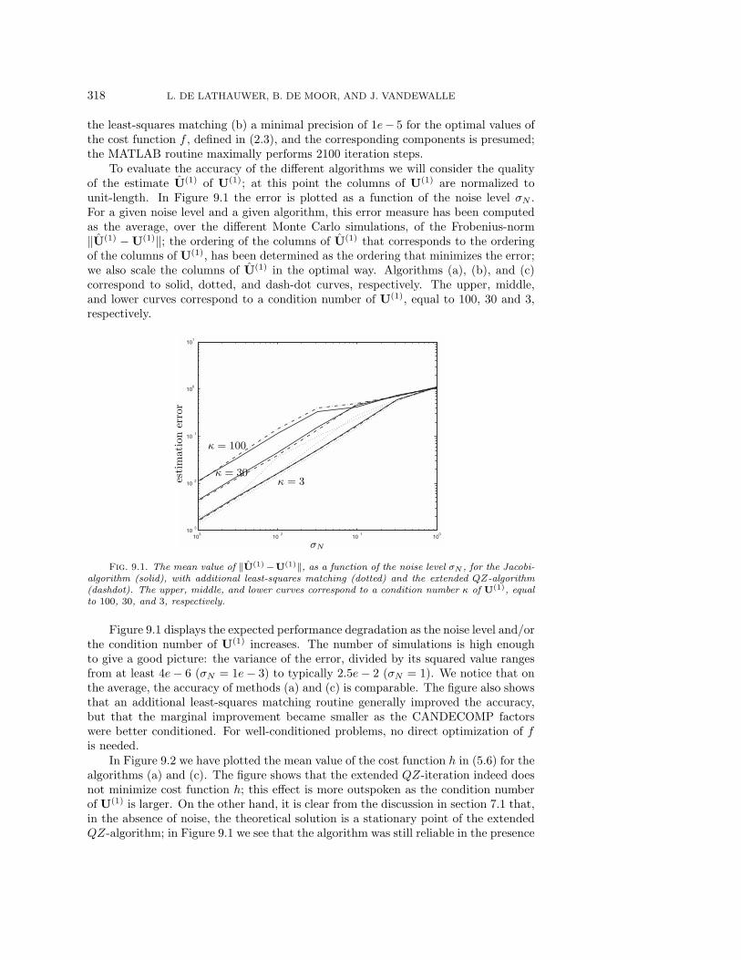
To evaluate the accuracy of the different algorithms we will consider the qualityof the estimate U(1) of U(1); at this point the columns of U(1) are normalized tounit-length. In Figure 9.1 the error is plotted as a function of the noise level σN .For a given noise level and a given algorithm, this error measure has been computedas the average, over the different Monte Carlo simulations, of the Frobenius-norm‖U(1) − U(1)‖; the ordering of the columns of U(1) that corresponds to the orderingof the columns of U(1), has been determined as the ordering that minimizes the error;we also scale the columns of U(1) in the optimal way. Algorithms (a), (b), and (c)correspond to solid, dotted, and dash-dot curves, respectively. The upper, middle,and lower curves correspond to a condition number of U(1), equal to 100, 30 and 3,respectively.
103
10 2
10 1
100
10 3
10 2
10 1
100
101
κ = 3κ = 30
κ = 100
σN
esti
mati
on
erro
r
Fig. 9.1. The mean value of ‖U(1) −U(1)‖, as a function of the noise level σN , for the Jacobi-algorithm (solid), with additional least-squares matching (dotted) and the extended QZ-algorithm(dashdot). The upper, middle, and lower curves correspond to a condition number κ of U(1), equalto 100, 30, and 3, respectively.
Figure 9.1 displays the expected performance degradation as the noise level and/orthe condition number of U(1) increases. The number of simulations is high enoughto give a good picture: the variance of the error, divided by its squared value rangesfrom at least 4e− 6 (σN = 1e− 3) to typically 2.5e− 2 (σN = 1). We notice that onthe average, the accuracy of methods (a) and (c) is comparable. The figure also showsthat an additional least-squares matching routine generally improved the accuracy,but that the marginal improvement became smaller as the CANDECOMP factorswere better conditioned. For well-conditioned problems, no direct optimization of fis needed.
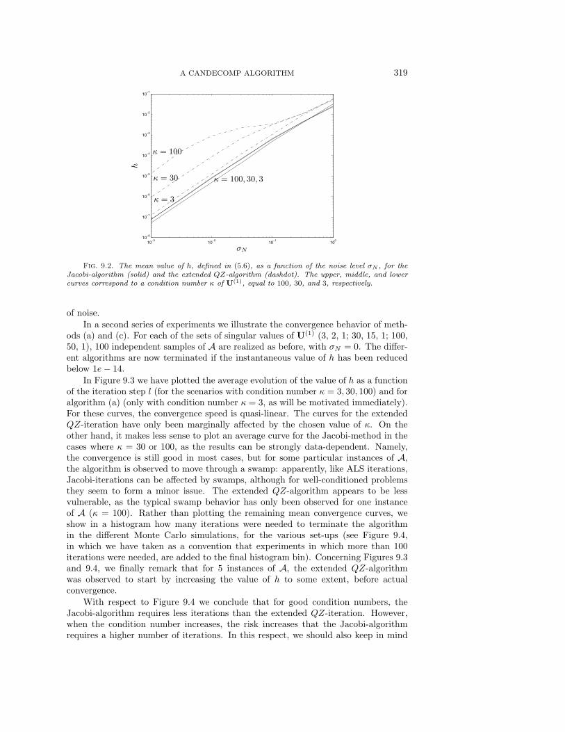
In Figure 9.2 we have plotted the mean value of the cost function h in (5.6) for thealgorithms (a) and (c). The figure shows that the extended QZ-iteration indeed doesnot minimize cost function h; this effect is more outspoken as the condition numberof U(1) is larger. On the other hand, it is clear from the discussion in section 7.1 that,in the absence of noise, the theoretical solution is a stationary point of the extendedQZ-algorithm; in Figure 9.1 we see that the algorithm was still reliable in the presence
A CANDECOMP ALGORITHM 319
10−3
10−2
10−1
100
10−8
10−7
10−6
10−5
10−4
10−3
10−2
10−1
κ = 3
κ = 30
κ = 100
κ = 100, 30, 3
σN
h
Fig. 9.2. The mean value of h, defined in (5.6), as a function of the noise level σN , for theJacobi-algorithm (solid) and the extended QZ-algorithm (dashdot). The upper, middle, and lowercurves correspond to a condition number κ of U(1), equal to 100, 30, and 3, respectively.
of noise.
In a second series of experiments we illustrate the convergence behavior of meth-ods (a) and (c). For each of the sets of singular values of U(1) (3, 2, 1; 30, 15, 1; 100,50, 1), 100 independent samples of A are realized as before, with σN = 0. The differ-ent algorithms are now terminated if the instantaneous value of h has been reducedbelow 1e− 14.
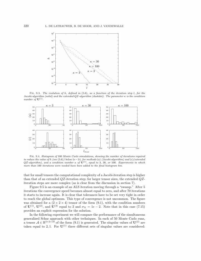
In Figure 9.3 we have plotted the average evolution of the value of h as a functionof the iteration step l (for the scenarios with condition number κ = 3, 30, 100) and foralgorithm (a) (only with condition number κ = 3, as will be motivated immediately).For these curves, the convergence speed is quasi-linear. The curves for the extendedQZ-iteration have only been marginally affected by the chosen value of κ. On theother hand, it makes less sense to plot an average curve for the Jacobi-method in thecases where κ = 30 or 100, as the results can be strongly data-dependent. Namely,the convergence is still good in most cases, but for some particular instances of A,the algorithm is observed to move through a swamp: apparently, like ALS iterations,Jacobi-iterations can be affected by swamps, although for well-conditioned problemsthey seem to form a minor issue. The extended QZ-algorithm appears to be lessvulnerable, as the typical swamp behavior has only been observed for one instanceof A (κ = 100). Rather than plotting the remaining mean convergence curves, weshow in a histogram how many iterations were needed to terminate the algorithmin the different Monte Carlo simulations, for the various set-ups (see Figure 9.4,in which we have taken as a convention that experiments in which more than 100iterations were needed, are added to the final histogram bin). Concerning Figures 9.3and 9.4, we finally remark that for 5 instances of A, the extended QZ-algorithmwas observed to start by increasing the value of h to some extent, before actualconvergence.
With respect to Figure 9.4 we conclude that for good condition numbers, theJacobi-algorithm requires less iterations than the extended QZ-iteration. However,when the condition number increases, the risk increases that the Jacobi-algorithmrequires a higher number of iterations. In this respect, we should also keep in mind
320 L. DE LATHAUWER, B. DE MOOR, AND J. VANDEWALLE
0 5 10 15 20 25 3010
−14
10−12
10−10
10−8
10−6
10−4
10−2
100
κ = 3κ = 3
κ = 30
κ = 100
l
h
Fig. 9.3. The evolution of h, defined in (5.6), as a function of the iteration step l, for theJacobi-algorithm (solid) and the extended QZ-algorithm (dashdot). The parameter κ is the conditionnumber of U(1).
50
50
50
50
50
50
50
4040
40
404040
40
40
3030
303030
30
2020
20
202020
20
20
1010
101010
10
00
00
00
00
00
00100
100100
100
κ = 3 κ = 30 κ = 100
lmax
(a)
(c)
Fig. 9.4. Histogram of 100 Monte Carlo simulations, showing the number of iterations requiredto reduce the value of h (see (5.6)) below 1e−14, for methods (a) (Jacobi-algorithm) and (c)(extendedQZ-algorithm), and a condition number κ of U(1), equal to 3, 30, or 100. Experiments in whichmore than 100 iterations were needed have been added to the final histogram bin.
that for small tensors the computational complexity of a Jacobi-iteration step is higherthan that of an extended QZ-iteration step; for larger tensor sizes, the extended QZ-iteration steps are more complex (as is clear from the discussion in section 7).
Figure 9.5 is an example of an ALS iteration moving through a “swamp.” After 5iterations the convergence speed becomes almost equal to zero, and after 70 iterationsit starts to increase again. It is clear that tolerances have to be set very tight in orderto reach the global optimum. This type of convergence is not uncommon. The figurewas obtained for a (2 × 2 × 4) tensor of the form (9.1), with the condition numbersof U(1), U(2), and U(3) equal to 2 and σN = 1e − 2. Note that in this case (7.15)provides an explicit expression for the solution.
In the following experiment we will compare the performance of the simultaneousgeneralized Schur approach with other techniques. In each of 50 Monte Carlo runs,a tensor A ∈ R
2×2×10 of the form (9.1) is generated. The singular values of U(2) aretaken equal to 2, 1. For U(1) three different sets of singular values are considered:
A CANDECOMP ALGORITHM 321
0 10 20 30 40 50 60 70 80 90 1000
0.1
0.2
0.3
0.4
0.5
0.6
0.7
0.8
0.9
1
f
l
Fig. 9.5. Example of a “swamp”-type convergence curve for ALS iterations. f is the costfunction defined in (2.3) and l the iteration step.
2,1; 10,1; 100,1. The entries of U(3) are generated as u(3)ij = 1 + gij/50, in which gij
is drawn from a Gaussian distribution with unit variance. For each particular choiceof U(1), U(2), U(3), and N , the scalar σN is varied between 1e − 4 and 1e − 2. Inthis way, σN ranges from a level where the eigenvalues in (4.10) are subject only to asmall perturbation to a level where there is a certain risk that these eigenvalues havecrossed each other.
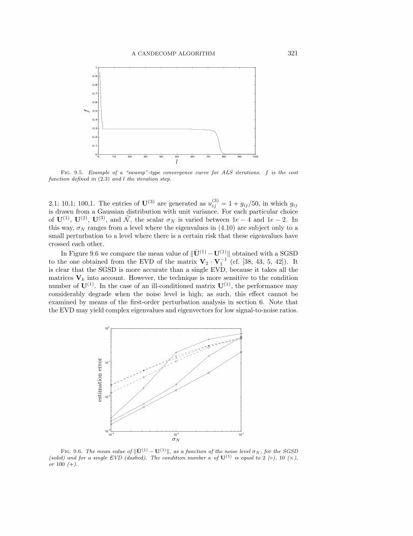
In Figure 9.6 we compare the mean value of ‖U(1)−U(1)‖ obtained with a SGSDto the one obtained from the EVD of the matrix V2 · V−1
1 (cf. [38, 43, 5, 42]). Itis clear that the SGSD is more accurate than a single EVD, because it takes all thematrices Vk into account. However, the technique is more sensitive to the conditionnumber of U(1). In the case of an ill-conditioned matrix U(1), the performance mayconsiderably degrade when the noise level is high; as such, this effect cannot beexamined by means of the first-order perturbation analysis in section 6. Note thatthe EVD may yield complex eigenvalues and eigenvectors for low signal-to-noise ratios.
10−4
10−3
10−2
10−3
10−2
10−1
100
σN
esti
mati
on
erro
r
Fig. 9.6. The mean value of ‖U(1) −U(1)‖, as a function of the noise level σN , for the SGSD(solid) and for a single EVD (dashed). The condition number κ of U(1) is equal to 2 (), 10 (×),or 100 (+).
322 L. DE LATHAUWER, B. DE MOOR, AND J. VANDEWALLE
10−4
10−3
10−2
10−3
10−2
10−1
100
σN
esti
mati
on
erro
r
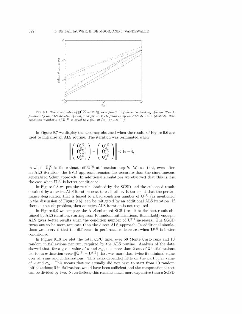
Fig. 9.7. The mean value of ‖U(1) −U(1)‖, as a function of the noise level σN , for the SGSD,followed by an ALS iteration (solid) and for an EVD followed by an ALS iteration (dashed). Thecondition number κ of U(1) is equal to 2 (), 10 (×), or 100 (+).
In Figure 9.7 we display the accuracy obtained when the results of Figure 9.6 areused to initialize an ALS routine. The iteration was terminated when∥∥∥∥∥∥∥
⎛⎜⎝ U
(1)k+1
U(2)k+1
U(3)k+1
⎞⎟⎠−
⎛⎜⎝ U
(1)k
U(2)k
U(3)k
⎞⎟⎠∥∥∥∥∥∥∥ < 1e− 4,
in which U(i)k is the estimate of U(i) at iteration step k. We see that, even after
an ALS iteration, the EVD approach remains less accurate than the simultaneousgeneralized Schur approach. In additional simulations we observed that this is lessthe case when U(3) is better conditioned.
In Figure 9.8 we put the result obtained by the SGSD and the enhanced resultobtained by an extra ALS iteration next to each other. It turns out that the perfor-mance degradation that is linked to a bad condition number of U(1) (as mentionedin the discussion of Figure 9.6), can be mitigated by an additional ALS iteration. Ifthere is no such problem, then an extra ALS iteration is not required.
In Figure 9.9 we compare the ALS-enhanced SGSD result to the best result ob-tained by ALS iteration, starting from 10 random initializations. Remarkably enough,ALS gives better results when the condition number of U(1) increases. The SGSDturns out to be more accurate than the direct ALS approach. In additional simula-tions we observed that the difference in performance decreases when U(3) is betterconditioned.
In Figure 9.10 we plot the total CPU time, over 50 Monte Carlo runs and 10random initializations per run, required by the ALS routine. Analysis of the datashowed that, for a given value of κ and σN , not more than 2 out of 3 initializationsled to an estimation error ‖U(1) −U(1)‖ that was more than twice its minimal valueover all runs and initializations. This ratio depended little on the particular valueof κ and σN . This means that we actually did not have to start from 10 randominitializations; 5 initializations would have been sufficient and the computational costcan be divided by two. Nevertheless, this remains much more expensive than a SGSD
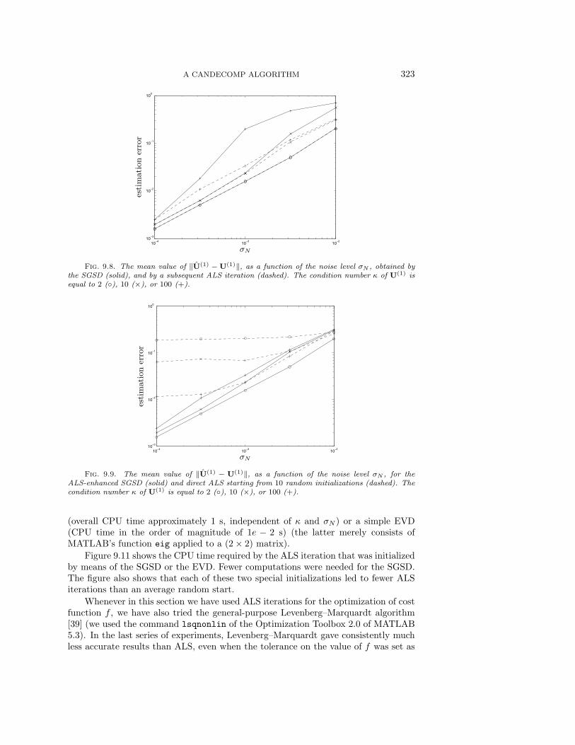
A CANDECOMP ALGORITHM 323
10−4
10−3
10−2
10−3
10−2
10−1
100
σN
esti
mati
on
erro
r
Fig. 9.8. The mean value of ‖U(1) − U(1)‖, as a function of the noise level σN , obtained bythe SGSD (solid), and by a subsequent ALS iteration (dashed). The condition number κ of U(1) isequal to 2 (), 10 (×), or 100 (+).
10−4
10−3
10−2
10−3
10−2
10−1
100
σN
esti
mati
on
erro
r
Fig. 9.9. The mean value of ‖U(1) − U(1)‖, as a function of the noise level σN , for theALS-enhanced SGSD (solid) and direct ALS starting from 10 random initializations (dashed). Thecondition number κ of U(1) is equal to 2 (), 10 (×), or 100 (+).
(overall CPU time approximately 1 s, independent of κ and σN ) or a simple EVD(CPU time in the order of magnitude of 1e − 2 s) (the latter merely consists ofMATLAB’s function eig applied to a (2 × 2) matrix).
Figure 9.11 shows the CPU time required by the ALS iteration that was initializedby means of the SGSD or the EVD. Fewer computations were needed for the SGSD.The figure also shows that each of these two special initializations led to fewer ALSiterations than an average random start.
Whenever in this section we have used ALS iterations for the optimization of costfunction f , we have also tried the general-purpose Levenberg–Marquardt algorithm[39] (we used the command lsqnonlin of the Optimization Toolbox 2.0 of MATLAB5.3). In the last series of experiments, Levenberg–Marquardt gave consistently muchless accurate results than ALS, even when the tolerance on the value of f was set as
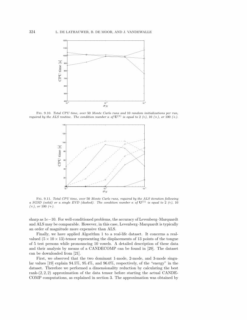
324 L. DE LATHAUWER, B. DE MOOR, AND J. VANDEWALLE
10−4
10−3
10−2
400
500
600
700
800
900
1000
1100
1200
σN
CP
Uti
me
[s]
Fig. 9.10. Total CPU time, over 50 Monte Carlo runs and 10 random initializations per run,required by the ALS routine. The condition number κ of U(1) is equal to 2 (), 10 (×), or 100 (+).
10−4
10−3
10−2
0
20
40
60
80
100
120
140
σN
CP
Uti
me
[s]
Fig. 9.11. Total CPU time, over 50 Monte Carlo runs, required by the ALS iteration followinga SGSD (solid) or a single EVD (dashed). The condition number κ of U(1) is equal to 2 (), 10(×), or 100 (+).
sharp as 1e−10. For well-conditioned problems, the accuracy of Levenberg–Marquardtand ALS may be comparable. However, in this case, Levenberg–Marquardt is typicallyan order of magnitude more expensive than ALS.
Finally, we have applied Algorithm 1 to a real-life dataset. It concerns a real-valued (5× 10× 13)-tensor representing the displacements of 13 points of the tongueof 5 test persons while pronouncing 10 vowels. A detailed description of these dataand their analysis by means of a CANDECOMP can be found in [29]. The datasetcan be downloaded from [21].
First, we observed that the two dominant 1-mode, 2-mode, and 3-mode singu-lar values [19] explain 94.5%, 95.4%, and 96.0%, respectively, of the “energy” in thedataset. Therefore we performed a dimensionality reduction by calculating the bestrank-(2, 2, 2) approximation of the data tensor before starting the actual CANDE-COMP computations, as explained in section 3. The approximation was obtained by
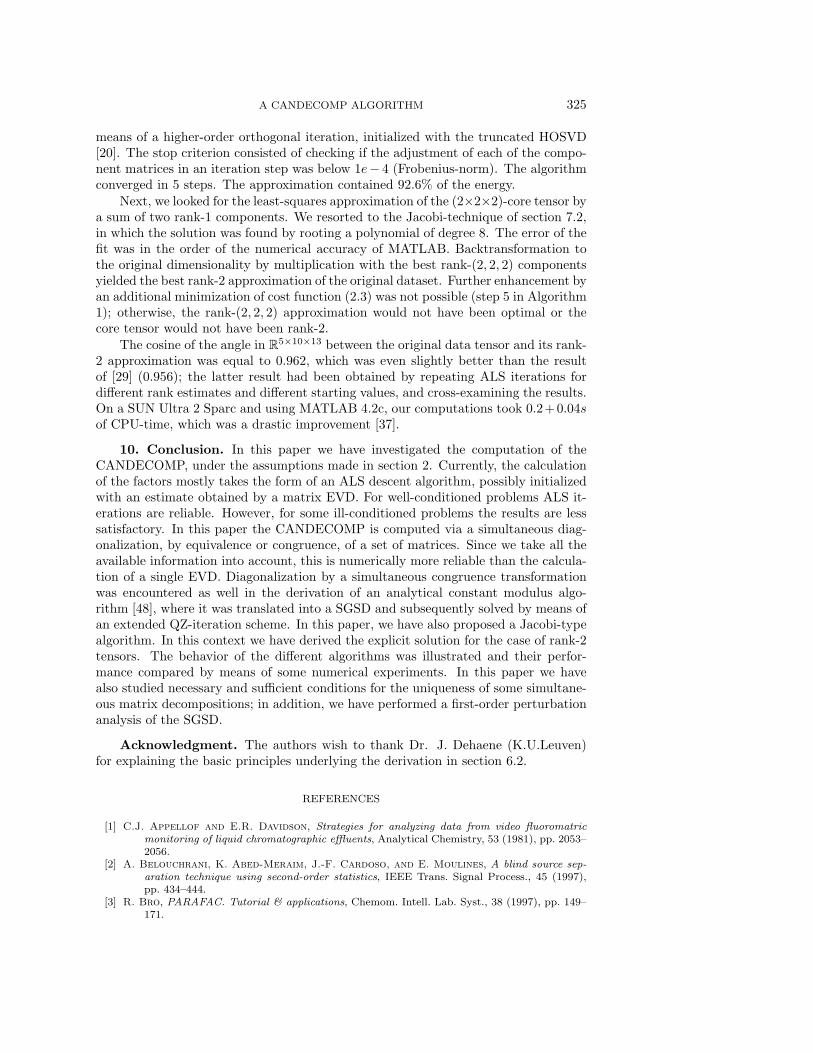
A CANDECOMP ALGORITHM 325
means of a higher-order orthogonal iteration, initialized with the truncated HOSVD[20]. The stop criterion consisted of checking if the adjustment of each of the compo-nent matrices in an iteration step was below 1e− 4 (Frobenius-norm). The algorithmconverged in 5 steps. The approximation contained 92.6% of the energy.
Next, we looked for the least-squares approximation of the (2×2×2)-core tensor bya sum of two rank-1 components. We resorted to the Jacobi-technique of section 7.2,in which the solution was found by rooting a polynomial of degree 8. The error of thefit was in the order of the numerical accuracy of MATLAB. Backtransformation tothe original dimensionality by multiplication with the best rank-(2, 2, 2) componentsyielded the best rank-2 approximation of the original dataset. Further enhancement byan additional minimization of cost function (2.3) was not possible (step 5 in Algorithm1); otherwise, the rank-(2, 2, 2) approximation would not have been optimal or thecore tensor would not have been rank-2.
The cosine of the angle in R5×10×13 between the original data tensor and its rank-
2 approximation was equal to 0.962, which was even slightly better than the resultof [29] (0.956); the latter result had been obtained by repeating ALS iterations fordifferent rank estimates and different starting values, and cross-examining the results.On a SUN Ultra 2 Sparc and using MATLAB 4.2c, our computations took 0.2+0.04sof CPU-time, which was a drastic improvement [37].
10. Conclusion. In this paper we have investigated the computation of theCANDECOMP, under the assumptions made in section 2. Currently, the calculationof the factors mostly takes the form of an ALS descent algorithm, possibly initializedwith an estimate obtained by a matrix EVD. For well-conditioned problems ALS it-erations are reliable. However, for some ill-conditioned problems the results are lesssatisfactory. In this paper the CANDECOMP is computed via a simultaneous diag-onalization, by equivalence or congruence, of a set of matrices. Since we take all theavailable information into account, this is numerically more reliable than the calcula-tion of a single EVD. Diagonalization by a simultaneous congruence transformationwas encountered as well in the derivation of an analytical constant modulus algo-rithm [48], where it was translated into a SGSD and subsequently solved by means ofan extended QZ-iteration scheme. In this paper, we have also proposed a Jacobi-typealgorithm. In this context we have derived the explicit solution for the case of rank-2tensors. The behavior of the different algorithms was illustrated and their perfor-mance compared by means of some numerical experiments. In this paper we havealso studied necessary and sufficient conditions for the uniqueness of some simultane-ous matrix decompositions; in addition, we have performed a first-order perturbationanalysis of the SGSD.
Acknowledgment. The authors wish to thank Dr. J. Dehaene (K.U.Leuven)for explaining the basic principles underlying the derivation in section 6.2.
REFERENCES
[1] C.J. Appellof and E.R. Davidson, Strategies for analyzing data from video fluoromatricmonitoring of liquid chromatographic effluents, Analytical Chemistry, 53 (1981), pp. 2053–2056.
[2] A. Belouchrani, K. Abed-Meraim, J.-F. Cardoso, and E. Moulines, A blind source sep-aration technique using second-order statistics, IEEE Trans. Signal Process., 45 (1997),pp. 434–444.
[3] R. Bro, PARAFAC. Tutorial & applications, Chemom. Intell. Lab. Syst., 38 (1997), pp. 149–171.
326 L. DE LATHAUWER, B. DE MOOR, AND J. VANDEWALLE
[4] A. Bunse-Gerstner, R. Byers, and V. Mehrmann, Numerical methods for simultaneousdiagonalization, SIAM J. Matrix Anal. Appl., 14 (1993), pp. 927–949.
[5] D. Burdick, X. Tu, L. McGown, and D. Millican, Resolution of multicomponent fluorescentmixtures by analysis of the excitation-emission-frequency array, J. Chemometrics, 4 (1990),pp. 15–28.
[6] J.-F. Cardoso, Super-symmetric decomposition of the fourth-order cumulant tensor. Blindidentification of more sources than sensors, in Proceedings of the IEEE International Con-ference on Acoustics, Speech, and Signal Processing, Toronto, Canada, 1991, pp. 3109–3112.
[7] J.-F. Cardoso, Iterative techniques for blind source separation using only fourth-order cumu-lants, in Signal Processing VI: Theories and Applications, Proc. EUSIPCO-92, Brussels,Belgium, 1992, pp. 739–742.
[8] J.-F. Cardoso and A. Souloumiac, Blind beamforming for non-Gaussian signals, IEE Proc.-F, 140 (1994), pp. 362–370.
[9] J.-F. Cardoso and A. Souloumiac, Jacobi angles for simultaneous diagonalization, SIAM J.Matrix Anal. Appl., 17 (1996), pp. 161–164.
[10] J. Carroll and J. Chang, Analysis of individual differences in multidimensional scalingvia an N-way generalization of “Eckart-Young” decomposition, Psychometrika, 9 (1970),pp. 267–283.
[11] J. Carroll, G. Desoete, and S. Pruzansky, An evaluation of five algorithms for generatingan initial configuration for SINDSCAL, J. Classification, 6 (1989), pp. 105–119.
[12] M.T. Chu, A continuous Jacobi-like approach to the simultaneous reduction of real matrices,Linear Algebra Appl., 147 (1991), pp. 75–96.
[13] P. Comon, Independent component analysis, a new concept? Signal Process., 36 (1994),pp. 287–314.
[14] P. Comon and B. Mourrain, Decomposition of quantics in sums of powers of linear forms,Signal Process., 53 (1996), pp. 93–108.
[15] J. Dehaene, Continuous-Time Matrix Algorithms, Systolic Algorithms and Adaptive NeuralNetworks, Ph.D. Thesis, E.E. Dept. (ESAT), K.U.Leuven, Belgium, 1995.
[16] L. De Lathauwer, B. De Moor, and J. Vandewalle, Independent component analysis basedon higher-order statistics only, in Proceedings of the IEEE Signal Processing Workshop onStatistical Signal and Array Processing, Corfu, Greece, 1996, pp. 356–359.
[17] L. De Lathauwer, Signal Processing Based on Multilinear Algebra, Ph.D. thesis, K.U. Leuven,E.E. Dept. (ESAT), Belgium, 1997.
[18] L. De Lathauwer, B. De Moor, and J. Vandewalle, Jacobi-algorithm for simultaneousgeneralized Schur decomposition in higher-order-only ICA, in Proceedings of the IEEEBenelux Signal Processing Chapter Signal Processing Symposium (SPS’98), Leuven, Bel-gium, 1998, pp. 67–70.
[19] L. De Lathauwer, B. De Moor, and J. Vandewalle, A multilinear singular value decom-position, SIAM J. Matrix Anal. Appl., 21 (2000), pp. 1253–1278.
[20] L. De Lathauwer, B. De Moor, and J. Vandewalle, On the best rank-1 and rank-(R1, R2, . . . , RN ) approximation of higher-order tensors, SIAM J. Matrix Anal. Appl.,21 (2000), pp. 1324–1342.
[21] B. De Moor, Ed., Database for the Identification of Systems (DAISY), E.E. Dept.,ESAT/SCD, K.U.Leuven, Belgium, http://www.esat.kuleuven.ac.be/sista/daisy/.
[22] A. Edelman, T.A. Arias, and S.T. Smith, The geometry of algorithms with orthogonalityconstraints, SIAM J. Matrix Anal. Appl., 20 (1998), pp. 303–353.
[23] B. Flury, Common Principal Components & Related Multivariate Models, John Wiley & Sons,New York, 1988.
[24] G.H. Golub and C.F. Van Loan, Matrix Computations, 3rd ed., Johns Hopkins UniversityPress, Baltimore, MD, 1996.
[25] M. Haardt, K. Huper, J. Moore, and J. Nossek, Simultaneous Schur Decomposition of sev-eral matrices to achieve automatic pairing in multidimensional harmonic retrieval prob-lems, in Signal Processing VIII: Theories and Applications, Proceedings of EUSIPCO-96,Trieste, Italy, 1996, Vol. 1, pp. 531–534.
[26] R. Harshman, Foundations of the PARAFAC procedure: Model and conditions for an “ex-planatory” multi-mode factor analysis, UCLA Working Papers in Phonetics, 16 (1970),pp. 1–84.
[27] R.A. Harshman and M.E. Lundy, The PARAFAC model for three-way factor analysis andmultidimensional scaling, in Research Methods for Multimode Data Analysis, H.G. Law,C.W. Snyder, J.A. Hattie, and R.P. McDonald, eds., Praeger, NY, 1984, pp. 122–215.
[28] R.A. Harshman and M.E. Lundy, PARAFAC: Parallel factor analysis, Comput. Statist. Data
A CANDECOMP ALGORITHM 327
Anal., 18 (1994), pp. 39–72.[29] R. Harshman, P. Ladefoged, and L. Goldstein, Factor analysis of tongue shapes, J. Acoust.
Soc. Am., 62 (1977), pp. 693–707.[30] T. Kato, A Short Introduction to Perturbation Theory for Linear Operators, Springer-Verlag,
New York, 1982.[31] H. Kiers and W. Krijnen, An efficient algorithm for PARAFAC of three-way data with large
numbers of observational units, Psychometrika, 56 (1991), pp. 147–152.[32] E. Kofidis and P.A. Regalia, On the best rank-1 approximation of higher-order supersym-
metric tensors, SIAM J. Matrix Anal. Appl., 23 (2002), pp. 863–884.[33] T. Kolda, A counterexample to the possibility of an extension of the Eckart–Young low-rank
approximation theorem for the orthogonal rank tensor decomposition, SIAM J. MatrixAnal. Appl., 24 (2003), pp. 762–767.
[34] J.B. Kruskal, Three-way arrays: rank and uniqueness of trilinear decompositions, with appli-cation to arithmetic complexity and statistics, Linear Algebra Appl., 18 (1977), pp. 95–138.
[35] J.B. Kruskal, Rank, decomposition, and uniqueness for 3-way and N-way arrays, in MultiwayData Analysis, R. Coppi and S. Bolasco, eds., North-Holland, Amsterdam, 1989, pp. 7–18.
[36] J.B. Kruskal, R.A. Harshman, and M.E. Lundy, How 3-MFA data can cause degeneratePARAFAC solutions, among other relationships, in Multiway Data Analysis, R. Coppi andS. Bolasco, eds., North-Holland, Amsterdam, 1989, pp. 115–122.
[37] P. Ladefoged, personal communication, Linguistics Dept., UCLA, Los Angeles, CA, 1996.[38] S.E. Leurgans, R.T. Ross, and R.B. Abel, A decomposition for three-way arrays, SIAM J.
Matrix Anal. Appl., 14 (1993), pp. 1064–1083.[39] J.J. More, The Levenberg-Marquardt algorithm: implementation and theory, in Numerical
Analysis, Lecture Notes in Math. 630, G.A. Watson, ed., Springer-Verlag, Berlin, 1977,pp. 105–116.
[40] P. Paatero, A weighted non-negative least squares algorithm for three-way “PARAFAC” factoranalysis, Chemom. Intell. Lab. Syst., 38 (1997), pp. 223–242.
[41] W.S. Rayens and B.C. Mitchell, Two-factor degeneracies and a stabilization of PARAFAC,Chemom. Intell. Lab. Syst., 38 (1997), pp. 173–181.
[42] E. Sanchez and B.R. Kowalski, Tensorial resolution: A direct trilinear decomposition, J.Chemometrics, 4 (1990), pp. 29–45.
[43] R. Sands and F. Young, Component models for three-way data: An alternating least squaresalgorithm with optimal scaling features, Psychometrika, 45 (1980), pp. 39–67.
[44] R. Schmidt, A Signal Subspace Approach to Multiple Emitter Location and Spectral Estima-tion, Ph.D. thesis, Stanford University, 1981.
[45] N. Sidiropoulos, G. Giannakis, and R. Bro, Blind PARAFAC receivers for DS-CDMAsystems, IEEE Trans. Signal Process., 48 (2000), pp. 810–823.
[46] N. Sidiropoulos, R. Bro, and G. Giannakis, Parallel factor analysis in sensor array pro-cessing, IEEE Trans. Signal Process., 48 (2000), pp. 2377–2388.
[47] N. Sidiropoulos and R. Bro, On the uniqueness of multilinear decomposition of N-wayarrays, J. Chemometrics, 14 (2000), pp. 229–239.
[48] A.-J. van der Veen and A. Paulraj, An analytical constant modulus algorithm, IEEE Trans.Signal Process., 44 (1996), pp. 1136–1155.
[49] A. Yeredor, Non-orthogonal joint diagonalization in the least-squares sense with applicationin blind source separation, IEEE Trans. Signal Process., 50 (2002), pp. 1545–1553.
[50] T. Zhang and G.H. Golub, Rank-one approximation to high order tensors, SIAM J. MatrixAnal. Appl., 23 (2001), pp. 534–550.


![Rational Canonical Formbuzzard.ups.edu/...spring...canonical-form-present.pdfIntroductionk[x]-modulesMatrix Representation of Cyclic SubmodulesThe Decomposition TheoremRational Canonical](https://static.fdocuments.in/doc/165x107/6021fbf8c9c62f5c255e87f1/rational-canonical-introductionkx-modulesmatrix-representation-of-cyclic-submodulesthe.jpg)


![Canonical Decomposition of even higher order cumulant ... · position of q-th order (q 2) cumulants. The latter de- ... best rank-1 approximation of Higher Order (HO) arrays [2] is](https://static.fdocuments.in/doc/165x107/61423dee55c1d11d1b34119a/canonical-decomposition-of-even-higher-order-cumulant-position-of-q-th-order.jpg)

![Canonical polyadic decomposition of 3rd order semi ... · factor analysis [22] with applications to chemometrics, psychology and marketing research.Ontheotherhand,inthedomainofsignalprocessing,andmorepartic-](https://static.fdocuments.in/doc/165x107/5cec9a4688c99319498d759d/canonical-polyadic-decomposition-of-3rd-order-semi-factor-analysis-22.jpg)