Computation of Heat and Fluid Flow using Domain ...
99
Computation of Heat and Fluid Flow using Domain Decomposition Method A Project Report Submitted in Partial Fulfillment of the Requirements for the Degree of Bachelor of Technology by Parmar Harsharajsinh Birendrasinh and Rohan Agrawal to the DEPARTMENT OF MECHANICAL ENGINEERING INDIAN INSTITUTE OF TECHNOLOGY GUWAHATI GUWAHATI - 781039, ASSAM MAY 2019
Transcript of Computation of Heat and Fluid Flow using Domain ...
Computation of Heat and Fluid Flow using Domain Decomposition
Method
A Project Report Submitted
in Partial Fulfillment of the Requirements
for the Degree of
Bachelor of Technology
by
Parmar Harsharajsinh Birendrasinh
and
Rohan Agrawal
to the
DEPARTMENT OF MECHANICAL ENGINEERING
INDIAN INSTITUTE OF TECHNOLOGY GUWAHATI
GUWAHATI - 781039, ASSAM
MAY 2019


Dedicated to our parents for their unconditional love and support.


CERTIFICATE
This is to certify that the work contained in this thesis entitled “Computation of Heat
and Fluid Flow using Domain Decomposition Method” is a bonafide work of Parmar
Harsharajsinh Birendrasinh and Rohan Agrawal carried out in the Department of
Mechanical Engineering, Indian Institute of Technology Guwahati under my supervision and
that it has not been submitted elsewhere for a degree.
Supervisor: Dr.Madhusudhana R.Gavara
Assistant Professor,
May, 2019 Department of Mechanical Engineering,
Guwahati. Indian Institute of Technology Guwahati, Assam.
i


APPROVAL SHEET
This project report entitled ”Computation of Heat and Fluid Flow using Domain
Decomposition Method”, a bonafide work by Parmar Harsharajsinh Birendrasinh
and Rohan Agrawal is approved for the degree of Bachelor of Technology.
Examiners
Supervisor
Chairman
May, 2019 Department of Mechanical Engineering,
Guwahati. Indian Institute of Technology Guwahati, Assam.
i


DECLARATION
I declare that this written submission represents my ideas in my own words and where
others’ ideas or words have been included, I have adequately cited and referenced the original
sources. I also declare that I have adhered to all principles of academic honesty and integrity
and have not misrepresented or fabricated or falsified any idea/data/source in my submission.
I understand that any violation of the above will be cause for disciplinary action by the
Institute and can also evoke penal action from the sources which have thus not been properly
cited or from whom proper permission has not been taken when needed.
Parmar Harsharajsinh Birendrasinh
150103051
Rohan Agrawal
150103058
May 16, 2019
i


Abstract
This project is aimed to develop and parallelize CFD solvers for incompressible heat and
fluid flows. The solver for incompressible heat and fluid flows is based on spectral method.
The parallelization of these codes is done based on the domain decomposition method using
OpenMP. This project is mainly divided into two modules - developing spectral codes and
parallelization of FDM and spectral codes. FDM codes are parallelized to lay the foundation
for working on spectral codes for fluid flow and heat transfer.
In the first module, a solver is developed for conduction heat transfer problems. The
solver is validated using heat conduction problem for which analytical solution is available.
Then, a solver for fluid flow problems is developed and the solver is validated against channel
flows and lid driven cavity. Then the solver is extended for convective heat transfer and
the solver is validated for forced convection in lid driven cavity and natural convection in
differentially side heated cavity. The above solvers are for regular rectangular geometries. A
solver also is developed for conduction in a triangular solid plate and is validated successfully.
In the second module, parallelization of the codes for heat transfer and fluid flow is carried
out. This module consists of two parts involving parallelization of codes based on FDM and
spectral methods respectively. First, one dimensional and two dimensional heat conduction
problems are implemented by dividing the domain into smaller domains. The computation
of individual smaller domains is given to different processors. The parallelization is further
extended to channel flow and lid driven cavity problem. In these conduction problems for
1-D and 2-D, the discretization is carried out using both FDM and spectral methods. For
fluid flow problems the discretization is carried out using spectral methods.

Acknowledgement
We have diligently worked towards the accomplishment of the desired goals in this project
however, it would not have been possible without positive feedback and inputs from colleagues
and mentors. We would like to express our sincere thanks to all of them.
We would like to pay high regards to our supervisor Dr. Madhusudhana. R. Gavara for
his numerous valuable insights and guidance whenever it seemed like we were getting fixated
on a problem or deviating from our path.
We would also like to thank the supervising panel for their constructive judgements and
for suggesting enhancements in our algorithm. Their feedback on the results and validation
was instrumental in pushing our cognitive skills for performing on a high level of quality.
Finally, our sincere thanks also goes to our colleagues and everyone who has directly or
indirectly contributed to this work by suggesting references and novel ideas which gave us
alternative insights into our work.
i


Contents
List of Figures v
List of Tables viii
1 Introduction 1
1.1 Parallel Computing . . . . . . . . . . . . . . . . . . . . . . . . . . . . . . . . 2
1.1.1 Parallel Computing Memory Architecture . . . . . . . . . . . . . . . 2
1.1.2 Important Terms . . . . . . . . . . . . . . . . . . . . . . . . . . . . . 4
1.2 Spectral Methods . . . . . . . . . . . . . . . . . . . . . . . . . . . . . . . . . 5
1.3 Literature Review . . . . . . . . . . . . . . . . . . . . . . . . . . . . . . . . . 6
1.4 Current Emphasis . . . . . . . . . . . . . . . . . . . . . . . . . . . . . . . . . 7
1.5 Problems Solved . . . . . . . . . . . . . . . . . . . . . . . . . . . . . . . . . 7
1.6 Organization of The Report . . . . . . . . . . . . . . . . . . . . . . . . . . . 8
2 CFD Computations using Spectral Methods 9
2.1 Mathematical Treatment . . . . . . . . . . . . . . . . . . . . . . . . . . . . . 9
2.1.1 Governing Equations . . . . . . . . . . . . . . . . . . . . . . . . . . . 9
2.1.2 Spatial Discretization . . . . . . . . . . . . . . . . . . . . . . . . . . . 10
2.1.3 Temporal Discretization . . . . . . . . . . . . . . . . . . . . . . . . . 12
2.1.4 Treatment for Triangular domains . . . . . . . . . . . . . . . . . . . . 14
2.2 Two Dimensional Heat Conduction . . . . . . . . . . . . . . . . . . . . . . . 16
iii

2.2.1 Physical System . . . . . . . . . . . . . . . . . . . . . . . . . . . . . . 16
2.2.2 Results and Validation . . . . . . . . . . . . . . . . . . . . . . . . . . 17
2.3 Channel Flow . . . . . . . . . . . . . . . . . . . . . . . . . . . . . . . . . . . 20
2.3.1 Physical System . . . . . . . . . . . . . . . . . . . . . . . . . . . . . . 20
2.3.2 Results . . . . . . . . . . . . . . . . . . . . . . . . . . . . . . . . . . . 21
2.4 Lid-driven Square Cavity . . . . . . . . . . . . . . . . . . . . . . . . . . . . . 22
2.4.1 Physical System . . . . . . . . . . . . . . . . . . . . . . . . . . . . . . 22
2.4.2 Results and Validation . . . . . . . . . . . . . . . . . . . . . . . . . . 24
2.5 Natural Convection . . . . . . . . . . . . . . . . . . . . . . . . . . . . . . . . 30
2.5.1 Physical System . . . . . . . . . . . . . . . . . . . . . . . . . . . . . . 30
2.5.2 Results . . . . . . . . . . . . . . . . . . . . . . . . . . . . . . . . . . . 31
2.6 Heat Conduction: Triangular Domain . . . . . . . . . . . . . . . . . . . . . . 32
2.6.1 Physical System . . . . . . . . . . . . . . . . . . . . . . . . . . . . . . 32
2.6.2 Results . . . . . . . . . . . . . . . . . . . . . . . . . . . . . . . . . . . 34
3 Parallelization of FDM Codes 35
3.1 1D Heat Conduction . . . . . . . . . . . . . . . . . . . . . . . . . . . . . . . 35
3.1.1 Jacobi Iterative Method . . . . . . . . . . . . . . . . . . . . . . . . . 36
3.1.2 Domain Decomposition in Space . . . . . . . . . . . . . . . . . . . . . 36
3.2 2D Heat Conduction . . . . . . . . . . . . . . . . . . . . . . . . . . . . . . . 39
3.2.1 TDMA Sweeps . . . . . . . . . . . . . . . . . . . . . . . . . . . . . . 40
3.2.2 Domain Decomposition with Two Sub-Domains . . . . . . . . . . . . 42
4 Parallelization of Spectral Codes 45
4.1 One Dimensional Heat Conduction . . . . . . . . . . . . . . . . . . . . . . . 45
4.1.1 Physical System . . . . . . . . . . . . . . . . . . . . . . . . . . . . . . 45
4.1.2 Results . . . . . . . . . . . . . . . . . . . . . . . . . . . . . . . . . . . 47
4.2 Two Dimensional Heat Conduction . . . . . . . . . . . . . . . . . . . . . . . 48
iv

4.2.1 Domain Decomposition with Two Subdomains . . . . . . . . . . . . . 48
4.2.2 Domain Decomposition with Four Subdomains . . . . . . . . . . . . . 51
4.3 Channel Flow . . . . . . . . . . . . . . . . . . . . . . . . . . . . . . . . . . . 56
4.3.1 Domain Decomposition with Two Subdomains . . . . . . . . . . . . . 56
4.3.2 Domain Decomposition with Four Subdomains . . . . . . . . . . . . . 59
4.4 Lid Driven Cavity . . . . . . . . . . . . . . . . . . . . . . . . . . . . . . . . . 64
4.4.1 Domain Decomposition with Two Subdomains . . . . . . . . . . . . . 64
4.4.2 Domain Decomposition with Four Subdomains . . . . . . . . . . . . . 67
5 Conclusions 71
5.1 Future Scope . . . . . . . . . . . . . . . . . . . . . . . . . . . . . . . . . . . 72
References 73
v

List of Figures
1.1 Shared Memory . . . . . . . . . . . . . . . . . . . . . . . . . . . . . . . . . . 3
1.2 Distributed Memory . . . . . . . . . . . . . . . . . . . . . . . . . . . . . . . 3
1.3 Hybrid Memory . . . . . . . . . . . . . . . . . . . . . . . . . . . . . . . . . . 4
2.1 2D Heat conduction . . . . . . . . . . . . . . . . . . . . . . . . . . . . . . . . 16
2.2 Temperature contours . . . . . . . . . . . . . . . . . . . . . . . . . . . . . . 18
2.3 Mid-line profile comparison . . . . . . . . . . . . . . . . . . . . . . . . . . . 18
2.4 2D Channel flow . . . . . . . . . . . . . . . . . . . . . . . . . . . . . . . . . 20
2.5 Velocity vectors . . . . . . . . . . . . . . . . . . . . . . . . . . . . . . . . . . 22
2.6 Lid-driven cavity . . . . . . . . . . . . . . . . . . . . . . . . . . . . . . . . . 23
2.7 Steady state streamlines comparison for Re = 100, 400 . . . . . . . . . . . . 27
2.8 Steady state streamlines comparison for Re = 1000, 2000 . . . . . . . . . . . 28
2.9 Variation of velocity along the center-line of the driven cavity for different Re 29
2.10 Natural convection in a square cavity . . . . . . . . . . . . . . . . . . . . . . 30
2.11 Comparison of streamfunction contours [a,b] and isotherms [c,d] for Ra = 107 32
2.12 Heat conduction in a triangular plate . . . . . . . . . . . . . . . . . . . . . . 33
2.13 Isotherms for the triangular plate . . . . . . . . . . . . . . . . . . . . . . . . 34
3.1 1D Heat conduction . . . . . . . . . . . . . . . . . . . . . . . . . . . . . . . . 35
3.2 Temperature distribution using Jacobi method . . . . . . . . . . . . . . . . . 37
3.3 Temperature distribution using domain decomposition . . . . . . . . . . . . 39
vii

3.4 2D Heat conduction . . . . . . . . . . . . . . . . . . . . . . . . . . . . . . . . 40
3.5 TDMA line-by-line method [Patankar [1]] . . . . . . . . . . . . . . . . . . . . 40
3.6 Temperature distribution using TDMA sweeps . . . . . . . . . . . . . . . . . 41
3.7 Temperature distribution using domain decomposition . . . . . . . . . . . . 43
4.1 1D Heat conduction . . . . . . . . . . . . . . . . . . . . . . . . . . . . . . . . 46
4.2 2D Heat conduction - two subdomains . . . . . . . . . . . . . . . . . . . . . 48
4.3 Midline profile comparison . . . . . . . . . . . . . . . . . . . . . . . . . . . . 50
4.4 Temperature contour plot for two subdomains . . . . . . . . . . . . . . . . . 51
4.5 2D Heat conduction - four subdomains . . . . . . . . . . . . . . . . . . . . . 52
4.6 Vertical midline profile comparison . . . . . . . . . . . . . . . . . . . . . . . 54
4.7 Horizontal midline profile comparison . . . . . . . . . . . . . . . . . . . . . . 54
4.8 Temperature contour plot for four subdomains . . . . . . . . . . . . . . . . . 55
4.9 Channel flow - two subdomains . . . . . . . . . . . . . . . . . . . . . . . . . 57
4.10 Combined grid layout for two subdomains . . . . . . . . . . . . . . . . . . . 57
4.11 Velocity vectors for channel flow with two subdomains . . . . . . . . . . . . 59
4.12 Channel flow - four subdomains . . . . . . . . . . . . . . . . . . . . . . . . . 60
4.13 Combined grid layout for four subdomains . . . . . . . . . . . . . . . . . . . 61
4.14 Velocity vectors for channel flow with four subdomains . . . . . . . . . . . . 63
4.15 Lid driven cavity - two subdomains . . . . . . . . . . . . . . . . . . . . . . . 65
4.16 Velocity vectors for lid driven flow at Re = 10 . . . . . . . . . . . . . . . . . 67
4.17 Lid driven cavity - four subdomains . . . . . . . . . . . . . . . . . . . . . . . 68
viii

List of Tables
2.1 Comparison of flow variable M1 for the square driven cavity at Re = 100. . . 25
2.2 Comparison of flow variable M2 for the square driven cavity at Re = 100. . . 25
2.3 Comparison of flow variable M1 for the square driven cavity at Re = 400. . . 26
2.4 Comparison of flow variable M2 for the square driven cavity at Re = 400. . . 26
3.1 Jacobi iterative method . . . . . . . . . . . . . . . . . . . . . . . . . . . . . . 36
3.2 Domain decomposition with two subdomains . . . . . . . . . . . . . . . . . . 37
3.3 Domain decomposition with four subdomains . . . . . . . . . . . . . . . . . 38
3.4 TDMA sweeps method . . . . . . . . . . . . . . . . . . . . . . . . . . . . . . 41
3.5 2D domain decomposition with two sub-domains . . . . . . . . . . . . . . . . 42
4.1 Comparison of serial, parallel times and speed-up over various grid sizes for
1D conduction. . . . . . . . . . . . . . . . . . . . . . . . . . . . . . . . . . . 47
4.2 Comparison of serial, parallel times and speed-up over various grid sizes for
2D conduction with two subdomains. . . . . . . . . . . . . . . . . . . . . . . 51
4.3 Comparison of serial, parallel times and speed-up over various grid sizes for
2D conduction with four subdomains. . . . . . . . . . . . . . . . . . . . . . . 55
4.4 Comparison of serial, parallel times and speed-up over various grid sizes for
channel flow with two subdomains. . . . . . . . . . . . . . . . . . . . . . . . 59
4.5 Comparison of serial, parallel times and speed-up over various grid sizes for
channel flow with four subdomains. . . . . . . . . . . . . . . . . . . . . . . . 63
ix

4.6 Comparison of serial, parallel times and speed-up over various grid sizes for
lid driven cavity with two subdomains. . . . . . . . . . . . . . . . . . . . . . 66
4.7 Comparison of serial, parallel times and speed-up over various grid sizes for
lid driven cavity with four subdomains. . . . . . . . . . . . . . . . . . . . . . 70
x

Nomenclature
α Thermal Diffusivity
Sgen Source term
ε Convergence limit
uk(t) time dependant expansion spectral coefficients
ν Kinematic Viscosity
ω vorticity
ψ stream function
ρ Density
V non-dimensional intermediate velocity vector at time (n+ 1)∆t
bx Body force in x-direction
by Body force in y-direction
ci coefficients to evaluate first derivative matrix D(1)
cp Specific heat capacity at constant pressure
D(1) Chebeyshev collocation first derivative matrix
D(1)ik coefficients of matrix D(1)
xi

Gr Grashof Number
hi(x) Lagrange polynomials
k Thermal Conductivity
N number of collocation points in x
P non-dimensional pressure field
p Pressure
Pr Prandtl Number
Q Heat flux
T Temperature
t Time
Tk(x) Chebyshev polynomials of order k
u Velocity component in the x-direction
uN(x, t) Polynomial approximation of degree N
V non-dimensional velocity vector
v Velocity component in the y-direction
xi Chebyshev-Gauss-Lobatto points
xii
Chapter 1
Introduction
Fluid flow and heat transfer are the central phenomena governing various physical processes.
Their understanding and visualization is important for designing components ranging from
micro-scale fuel cells to commercial power systems. Experimental and numerical approaches
serve to resolve the flow fields in various situations with each having their own benefits.
From an overall perspective, experiments and computations go hand-in-hand and complement
each other. In designing systems, computations are first carried out to consider numerous
variations and then experiments follow up to characterize their performance. On the other
hand for understanding novel flows, experiments precede computations to give insights on
their characteristics [1].
Numerical methods for solving PDEs have been developed since the 1950s with first
introductions to Finite Difference methods (FDM) [2]. Since then many more methods have
been devised with broader applications in fluid mechanics, structural analysis and other
diverse fields. Finite element method (FEM), Finite Volume method (FVM) and Spectral
methods have been used recently for solving flows. The FDM, FVM and FEM are local
methods and have a limited order of accuracy (2nd or 3rd order) promoting the need for
high accuracy solution methods. The present work fills this gap and focuses on formulating
high-accuracy Chebyshev Spectral codes for solving certain fundamental fluid flow and heat
1

transfer problems.
Traditional serial computing proves to be insufficient and may not be able to solve such
problems in reasonable time. In some situations large number of parametric studies need to
be performed to find the appropriate and optimal design values. In such applications the use
of multiple processors becomes essential to solve the problem in reasonable time. To facilate
the use of multiple processors to work concurrently on different tasks of the same problem
parallelization of the code is essential.
1.1 Parallel Computing
Parallel computing in its simplest sense is to make use of multiple computing resources which
may include multi-core processors or multi-processors inteconnected via a communication
network to solve complex computational problems which can be broken down into multiple
discrete pieces concurrently. Each part is then broken down to a set of instructions which
are then run on individual processor (Computing resource). Parallel computing can therefore
combine multiple resources to achieve high performance and very fast computing.
There are different ways to make use of computing resources concurrently which define
the different parallel computing architectures.
1.1.1 Parallel Computing Memory Architecture
Parallel computing memory architectures can be broadly classified as shared , distributed
and hybrid distributed-shared memory architectures.
• Shared Memory In shared memory parallel computers all processors have access to
all memory as global address space. Multiple processors can share the same memory
resources while operating independent of each other. Changes in a memory location
effected by one processor are visible to all other processors. This leads to two problems
which needs to be addressed while designing a shared memory system: Performance
2

degradation due to contention. Coherence problem. Shared memory architecture can
further be classified as Uniform Memory Access (UMA) and Non-Uniform Memory
Access (NUMA).
(a) UMA (b) NUMA
Fig. 1.1: Shared Memory
• Distributed Memory In distributed memory computers processors have their own
local memory which means there is no concept of global address space. Since memory
in one processor doesn’t map to another processor changes made by one are not visible
to the other. Therefore to communicate and synchronise data between inter-processor
memory a communication network is required which can vary widely and can simply
be ethernet. It becomes the responsibilty of the programmer to define how data
communication and synchronisation between tasks take place.
Fig. 1.2: Distributed Memory
• Hybrid Distributed-Shared Memory Hybrid distributed-shared memory architecture
employs both shared and distributed memory architectures. The shared memory
component can be a shared memory machine and/or graphics processing units (GPU)
3
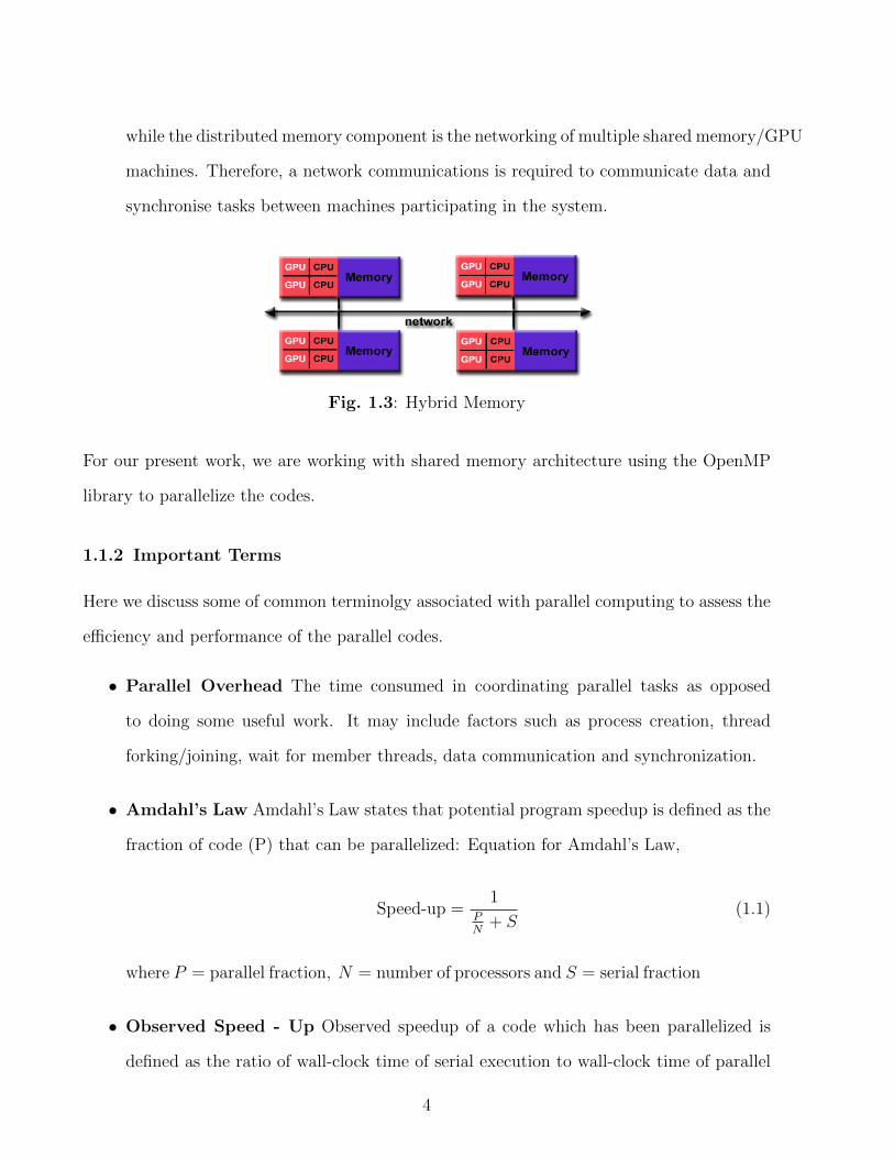
while the distributed memory component is the networking of multiple shared memory/GPU
machines. Therefore, a network communications is required to communicate data and
synchronise tasks between machines participating in the system.
Fig. 1.3: Hybrid Memory
For our present work, we are working with shared memory architecture using the OpenMP
library to parallelize the codes.
1.1.2 Important Terms
Here we discuss some of common terminolgy associated with parallel computing to assess the
efficiency and performance of the parallel codes.
• Parallel Overhead The time consumed in coordinating parallel tasks as opposed
to doing some useful work. It may include factors such as process creation, thread
forking/joining, wait for member threads, data communication and synchronization.
• Amdahl’s Law Amdahl’s Law states that potential program speedup is defined as the
fraction of code (P) that can be parallelized: Equation for Amdahl’s Law,
Speed-up =1
PN
+ S(1.1)
where P = parallel fraction, N = number of processors and S = serial fraction
• Observed Speed - Up Observed speedup of a code which has been parallelized is
defined as the ratio of wall-clock time of serial execution to wall-clock time of parallel
4

execution. Equation for Observed Speed-Up,
Observed speed-up =Wall-clock time of serial execution
Wall-clock time of parallel execution(1.2)
1.2 Spectral Methods
Spectral methods are higher-order accurate numerical methods that surfaced in solving PDEs
during the late 1970. The order of accuracy is said to be equal to the number of grid points
provided that the function to be approximated is smooth, analytic and non-singular. The
type of approximation used for the function forms a cardinal aspect in any spectral method.
On the lines of this, usually two types of Spectral methods are used in CFD:
• Fourier Spectral Methods - These are used in problems exhibiting a periodicity at
the boundaries
• Chebyshev Spectral Methods - These are used for problems having non-periodic
boundary conditions
These methods can be rendered useful particularly for regular domains and usually involve
mathematical and implementation-level difficulties when extended to arbitrary domains. Our
work is based on Chebyshev collocation form of spectral methods which use a pre-defined set
of grid points called Gauss-Lobatto points which form a biased grid with refinements near
the corners. Specifically, in case of finite domains with ”physical” boundary conditions, for
instance the no slip condition, polynomial basis functions (Chebyshev) lead to efficient and
accurate algorithms [3]. These characteristics are to be kept in mind when using this method
for practical problems.
5

1.3 Literature Review
Since the development of spectral methods in late 1970, a considerable amount of research
has been aimed at applying them in solving high-accuracy problems. C. Canuto et al. [4]
and D. Gottlieb et al. [5] considered the application of spectral methods in Direct Numerical
Simulations of turbulent flows. They also categorized the preferred type of spectral method
that is fourier or chebyshev depending on the boundary conditions of problems. Solomonoff
et al. [6] considered the global characteristics of psuedospectral methods and highlighted the
critical aspects to ensure correct solution procedure. Deville et al. [7] worked on deriving
the derivative matrices for chebyshev spectral methods.
Fluid flow problems are solved by using projection methods in conjunction with spectral
discretizations in this study and so a brief background on the developments on this side are
considered. Botella O. et al. [8] provided solutions to the Navier-Stokes equation using a
combination of spectral and temporal schemes. Chorin [9] and Temam [10] were the first ones
to propose the original form of projection method and since then several variants have been
devised. Huges et al. [11] were reportedly the first to use projection methods in combination
with spectral methods. Finally, Streett et al. [12] applied the semi-implicit projection method
to large-scale problems and also formulated a discretized version of the same.
Domain decomposition as a method for parallelization was pioneered in Computational
Fluid Dynamics by Gropp et al. [13]. They highlighted the benefits of domain decomposition
pertaining to its flexibility in containing adaptive refinements and its modular pathway to
parallelism. A simple classical problem of flow over a backstep was solved to illustrate these
features. Carvalho et al. [14] extended over this work and implemented a variation of domain
decomposition using overlapping sections of the subdomains. They reported an accelerated
convergence of the algorithm as a result of increased overlapping. Recent work by Nestola et
al. [15] implemented overlapping domain decomposition on an immersed boundary method
for fluid-structure interaction.
6

1.4 Current Emphasis
By virtue of their high accuracy, Spectral methods find application in scenarios where it is
necessary to solve the full Navier-Stokes equation. The full-solutions contribute to enhanced
understanding and knowledge about certain fundamental flow phenomena. Firstly, Direct
Numerical Simulation (DNS) of turbulent flows is an important application of spectral
methods. Secondly, they are also used in stability analysis where it is critical to refine
the base flow accurately for applying perturbations.
Presently, we are developing spectral codes that would be solved through a parallel
architecture and used for Large Eddy Simulations (LES). We have focused on developing
solution schemes for incompressible flows and tested them on certain fundamental fluid flow
and heat transfer problems. For parallelization, work has been done on TDMA sweeps and
Domain Decomposition. The results have been validated using available analytical solutions
and benchmark results in prevalent literature.
1.5 Problems Solved
The present work comprises of various test problems to validate our spectral code and they
are listed as follows,
• Two-dimensional heat Conduction in a rectangular plate
• Plane Poiseuille flow
• Lid-driven flow in a square cavity
• Natural convection in a square cavity
• Two-dimensional heat conduction in a triangular plate
7

1.6 Organization of The Report
This chapter provides a background for parallel computing. We have provided a description
of different architectures used in parallel computing. Then we described some of relevant
terms to study different algorithms for parallel programs. In the first half of this report,
spectral codes have been developed for solving fluid flow and heat transfer problems. The
parallelization part follows the code development and is divided into two parts - parallel
computing of FDM codes and parallel computing of Spectral codes.
Parallelization of FDM codes for the following problems is presented:
• One Dimensional Heat conduction
• Two Dimensional Heat conduction
Spectral codes for the following problems have been parallelized:
• One Dimensional Heat conduction
• Two Dimensional Heat conduction
• Channel flow
• Lid driven cavity
The computations proceed in a structured manner describing the governing equations,
spatial and temporal discretization and special treatment demanded by triangular domains.
Thereafter, the problems are considered and each one comprises of,
• Physical system description
• Governing equation under assumptions
• Results
• Conclusion
8

Chapter 2
CFD Computations using Spectral
Methods
2.1 Mathematical Treatment
2.1.1 Governing Equations
The problems discussed in this study are confined to two dimensions and so all the dimensional
form of governing equations have been expressed accordingly.
Heat Conduction
The two dimensional heat conduction equation can be represented as,
ρ cp∂T
∂t= k
(∂2T
∂x2+∂2T
∂y2
)+ Sgen
Fluid flow and Heat transfer
The dimensional form of governing equations can be represented as follows.
Continuity Equation,
∂u
∂x+∂v
∂y= 0
9

x-momentum equation,
∂u
∂t+ u
∂u
∂x+ v
∂u
∂y= −1
ρ
∂p
∂x+ ν
(∂2u
∂x2+∂2u
∂y2
)+ bx
y-momentum equation,
∂v
∂t+ u
∂v
∂x+ v
∂v
∂y= −1
ρ
∂p
∂y+ ν
(∂2v
∂x2+∂2v
∂y2
)+ by
Energy convection,
∂T
∂t+ u
∂T
∂x+ v
∂T
∂y= α
(∂2T
∂x2+∂2T
∂y2
)+ Sgen
For natural convection the governing equations change slightly and are usually expressed in
their non-dimensional form. The equations that change are expressed below:
x-momentum equation,
∂u
∂t+ u
∂u
∂x+ v
∂u
∂y= −∂p
∂x+ Pr
(∂2u
∂x2+∂2u
∂y2
)
y-momentum equation,
∂u
∂t+ u
∂u
∂x+ v
∂u
∂y= −∂p
∂x+ Pr
(∂2u
∂x2+∂2u
∂y2
)+GrPr2T
2.1.2 Spatial Discretization
The equations are spatially discretized using a Chebyshev collocation spectral method. The
collocation method has a characteristic that the numerical solution is forced to satisfy
governing equations exactly at the collocation points. Thereby if we wish to solve for a
10

function u(x, t) on the domain [-1,1] then it may be approximated as
uN(x, t) =N∑k=0
uk(t)Tk(x)
For the Chebyshev collocation method, Tk(x) represents chebyshev polynomials of order k.
The grids points serve for interpolation and are defined as the Chebyshev-Gauss-Lobatto
points,
xi = cos
(πi
N
)i = 0, 1, ....., N
These points correspond to extreme points of Chebyshev polynomials of order N,
TN(x) = cos(N cos−1 x
)The expansion coefficients, uk(t) may be evaluated using the inverse relation
uk(t) =2
Nck
N∑i=0
uN(xi, t)
cicos
(kπi
N
), k = 0, 1, ....., N
where ci and ck = 1 for i, k = 1, 2, ....., N − 1 and c0 = cN = 2.
The interpolation in collocation spectral method can also be expressed in terms of Lagrange
polynomials of order N , hi(x) such that hi(x) = δik, the Kronecker operator. The Lagrange
polynomials for the points considered may be represented by:
hi(x) =(−1)i+1(1− x2)T ′N(x)
ciN2(x− xi), i = 0, 1, ....., N
where ci = 1 for i = 1, ....., N − 1 and c0 = cN = 2.
11

The spatial derivative of uN(x, t) at the collocation points xi is evaluated using the
analytical derivatives of Lagrange polynomials,
u′N(xi, t) =N∑k=0
D(1)ik u(xk, t), i = 0, 1, ....., N
where D(1) is the Chebyshev collocation derivative matrix. It is given by the following
expression:
D(1)ik =
ci(−1)i+k
ck(xi − xk), i 6= k,
− xk2(1− x2
k), 1 ≤ i = k ≤ N − 1,
2N2 + 1
6, i = k = 0,
−2N2 + 1
6, i = k = N.
The Chebyshev collocation second derivative matrix D(2) can be obtained by following the
relation D(2) = (D(1))2. The higher order derivatives are obtained in a similar manner that
is by multiplying D(1) successively.
2.1.3 Temporal Discretization
Projection Method
Projection method belongs to the predictor-corrector class of algorithms and is non-iterative
in nature. Pressure acts as a projection of the predicted velocity field to form a divergence
free space in this class of methods. Spectral methods offer high accuracy but as is the case
with most numerical schemes, there is a trade-off between accuracy and stability. This implies
that spectral methods when used with ill-conditioned temporal schemes can lead to largely
unstable behaviour.
We have used a second-order semi-implicit time integration scheme and in addition the
12

spatial discretization is carried out using a Chebyshev collocation spectral method. The
time integration scheme is formed as a combination of Crank-Nicolson scheme acting on the
diffusive terms and Adams-Bashforth scheme acting on the convective terms. The projection
method partitions the solution of Navier-Stokes equations into two decoupled problems.
An intermediate velocity field is calculated using the Burgers equation and thereafter the
Poisson equation for pressure is used to correct the velocity field as to satisfy continuity. The
semi-implicit projection method discussed above can be described as follows:
a) Advection-Diffusion step which involves the intermediate velocity at (n+ 1)∆t, V
V − V n
∆t=
1
ReD(V )−NL(V ) in Ω
Boundary conditions for this intermediate velocity
τ · V = τ · V + τ ·∆t(2∇P n −∇P n−1) on ∂Ω
n · V = n · V on ∂Ω
Here NL(V ) = (V ·∇)V and D(V ) = ∇2V represent the advection and diffusion terms.
b) Pressure correction step solves the Poisson equation for P n+1
∇2P n+1 =∇ · V
∆tin Ω
With homogeneous Neumann boundary conditions
n · ∇P n+1 = 0 on ∂Ω
13
Thereafter the velocities are updated as given below,
V n+1 = V −∆t∇P n+1 in Ω + ∂Ω
The combination of an explicit second-order Adams-Bashforth scheme for the advection terms
and an implicit Crank-Nicolson scheme for diffusion terms can be described as follows.
NL(V ) =3
2NL(V n)− 1
2NL(V n−1)
D(V ) =D(V ) +D(V n)
2
These expressions are used in the Burgers equation at each time step.
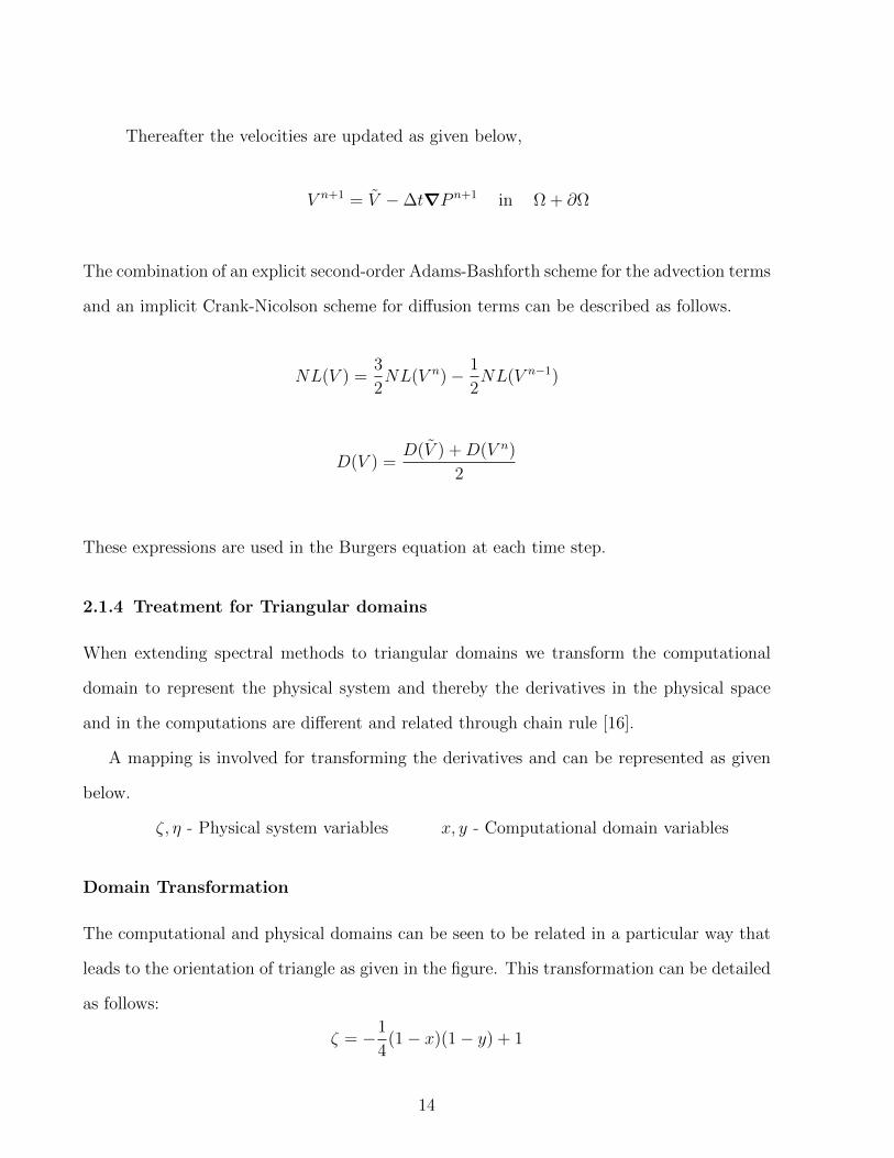
2.1.4 Treatment for Triangular domains
When extending spectral methods to triangular domains we transform the computational
domain to represent the physical system and thereby the derivatives in the physical space
and in the computations are different and related through chain rule [16].
A mapping is involved for transforming the derivatives and can be represented as given
below.
ζ, η - Physical system variables x, y - Computational domain variables
Domain Transformation
The computational and physical domains can be seen to be related in a particular way that
leads to the orientation of triangle as given in the figure. This transformation can be detailed
as follows:
ζ = −1
4(1− x)(1− y) + 1
14

η =1
2(y − 1)
The triangular domain so formed is given as (ζ, η) : 0 ≤ ζ ≤ 1,−1 ≤ η ≤ 0, ζ + η ≥ 0
mapped from the square computational domain.
The Inverse mapping is given as:
x =2(ζ − 1)
η + 1+ 1
y = 2η + 1
The derivatives can then be transformed and expressed as given below:
uζ =2
η + 1ux
uζζ =
(2
η + 1
)2
uxx
uη = −2(ζ − 1)
(η + 1)2ux + 2uy
uηη =4(ζ − 1)2
(η + 1)4uxx −
8(ζ − 1)
(η + 1)2uxy +
4(ζ − 1)
(η + 1)3ux + 4uyy
So finally the laplacian in the physical coordinates can be written in terms of those in the
computational domain as:
∆u =
(2
η + 1
)2
+4(ζ − 1)2
(η + 1)4
uxx −
8(ζ − 1)
(η + 1)2uxy +
4(ζ − 1)
(η + 1)3ux + 4uyy
This transformation has been applied to a heat conduction problem in a triangular plate
discussed in the subsequent sections.
15

2.2 Two Dimensional Heat Conduction
Heat conduction problems play an important role as preliminary tests for validating the code
structure and proper running. In this case we have considered a simple steady state problem
for which analytical solutions exist ensuring proper validation.
2.2.1 Physical System
The physical system consists of a square plate which has three adjacent sides at the same
temperature (Tc) as shown in Fig. 2.1. The remaining side is kept at a higher temperature
(Th) and the source terms are taken to be zero giving a source-less heat diffusion through the
plate.
Plate length is represented as L and width is represented as W. Constant temperatures
are applied at the four edges. Thermal diffusivity of the material is assumed to be unity as
it serves just a scaling factor as far as computations are concerned.
Fig. 2.1: 2D Heat conduction
The heat conduction is assumed to be steady and the effects from generation terms
16
have been neglected. The thermophysical properties are assumed to be independent of
temperature.
Governing Equation
Under the assumption of Steady state and zero generation in the plate the governing equation
reduces to a laplace equation.
∂2T
∂x2+∂2T
∂y2= 0
Boundary Conditions
At the left, right and bottom wall:
Tc = 300K
At the top wall:
Th = 400K
2.2.2 Results and Validation
Validation of the results is carried out by comparing with analytical solution available in
Holman [17], the expression of which is shown below:
T − TcTh − Tc
=2
π
∞∑n=1
(−1)n+1 + 1
nsin
nπx
W
sinh(nπy/W )
sinh(nπH/W )
Temperature values along a horizontal center line are calculated using the analytical expressions
and plotted along with the numerical results. An infinite sequence is surfaced in the exact
solution and so we have to limit it at a certain n to enable numerical computation of
temperatures. Cut-off limit is set by considering the difference between successive summation
series and the series is terminated when the difference goes below 10−12.The plot shown in
Fig. 2.3 gives the comparison along domain’s horizontal mid-line.
17

Fig. 2.2: Temperature contours
Fig. 2.3: Mid-line profile comparison
18

We observe that the mid-line numerical solution plot coincides exactly with the analytical
solution. This validation serves as an important check to guarantee that our solution
technique can accurately tackle the most fundamental problems. So we conclude from this
problem that our code can accurately handle pure diffusion and diffusion related terms in
general governing equations.
19

2.3 Channel Flow
Code for solving Incompressible fluid flow is validated using various test case studies. The
classical problems related to incompressible flows like 2D Channel flow and Lid-driven Cavity
flow are simulated to examine their accuracy.
The model represents a channel formed by placing two infinite plates parallel to each
other in the physical domain. A fully developed profile is used as inlet condition and the
emphasis is to resolve the convective terms accurately.
2.3.1 Physical System
Physical system consists of a 2D channel formed by placing two infinite plates parallel to
each other separated by a unit distance, as shown in Fig. 2.4. Flow is assumed to be fully
developed at the inlet and gradients along the downstream directions are set to zero for
velocity and pressure at the outlet. No-slip boundary conditions are imposed at the top and
bottom wall for velocity and the normal pressure gradients are set to zero.
Channel length is represented as L and width is represented as W . The flow Reynolds
number is set to 100 and a transient solution technique is adopted.
Fig. 2.4: 2D Channel flow
The flow is assumed to be time dependant and incompressible. Body forces are assumed
20

to be absent and fluid properties like density and viscosity are taken to be constants.
Boundary Conditions
A fully developed flow profile is fixed at the inlet and no-slip boundary condition is applied
at the walls. Streamwise gradients are set to zero for the velocity boundary conditions at the
outlet. For pressure, the gradients normal to surfaces are set to zero at the four boundaries.
The boundary conditions can be given in the mathematical format as shown below:
At top and bottom wall:
u = 0, v = 0,∂p
∂y= 0
At the left wall (inlet):
u = 1− y2, v = 0,∂p
∂x= 0
At the right wall (outlet):
∂u
∂x= 0,
∂v
∂x= 0,
∂p
∂x= 0
2.3.2 Results
Channel flow problem was solved for a Re = 100 and the velocity vectors were plotted to
visualize the flow profile at subsequent downstream positions as shown in Fig. 2.5.
The velocity vectors are in correspondence to our expectations and analytical solutions.
Thus in conclusion this problem validates passive transport handling capacity of our code
and we further move on to consider additional complications.
21

Fig. 2.5: Velocity vectors
2.4 Lid-driven Square Cavity
This is a classic problem for realizing internal recirculating flows within a bounded domain
and display several critical fluid flow phenomena in a relatively simplistic geometrical setting.
The physical model represents a square cavity with a driven lid on top to induce the
recirculation.
2.4.1 Physical System
A square cavity with lid on its top surface is considered as the physical model, as shown in
Fig. 2.6. The lid is assigned a horizontal velocity based on profile that remains consistent
with zero velocity at the extreme points. No-slip boundary condition is applied at three
remaining boundaries. Gradients of pressure normal to the boundaries are set to zero with a
special treatment considered later.
The cavity length is defined as L while the height is specified as W . Non-dimensional form
of Navier-Stokes equation is used for this problem and so fluid properties have been included
in the Reynolds Number. Change in Reynolds number would reflect different working fluids.
Flow is assumed to be incompressible and a transient analysis is carried out. Body forces
22

Fig. 2.6: Lid-driven cavity
have been neglected and it is valid to assume the characteristic length as the lid dimension.
Characteristic velocity is taken to be the average velocity over the lid.
Boundary Conditions
Lid is driven at a velocity which varies along its length and is zero at the boundaries so as
to be conformal. Rest of the boundaries are supplied with no-slip conditions.
We had an interesting observation for the pressure boundary conditions which involve
gradients at each side. Incompressible flows deal with the gradients of pressure at every stage
and the values of pressure themselves do not have any role here. Even in this problem we
have a poisson equation governing pressure and the boundary conditions work with gradients.
But, in solving the equations numerically pressure becomes unconstrained and it is thereby
advised to set the pressure as zero at a point in the computational domain. We have set the
pressure to be zero at the square’s center.
At left and right wall:
u = 0, v = 0,∂p
∂x= 0
At the bottom wall:
u = 0, v = 0,∂p
∂y= 0
23

At the lid:
u = 16x2(1− x2), v = 0,∂p
∂y= 0
At the domain’s center point:
p = 0
2.4.2 Results and Validation
The computations have been carried out at a range of Reynolds number starting from 100 to
2000. Additional definitions of streamfunction and vorticity are introduced in post processing
to examine the streamlines and for quantitative validation.
Vorticity is computed at each time step using,
ωn+1 =∂vn+1
∂x− ∂un+1
∂y
The streamfunction ψ is computed using the Poisson equation,
∇2ψn+1 = −ωn+1 in Ω
ψn+1 = 0 on ∂Ω
The results were qualitatively validated by comparing the streamfunction contours and
the center-line velocity profiles with previous work by Martinez et al, as shown in Fig. 2.7,
Fig. 2.8 and Fig. 2.9. N represents elements in the x-direction and M represents y-direction
elements. A mesh of 33 × 33 has been used with a time step of 10−3 to guarantee high
precision of the results and stability of the method. The Chebyshev-Gauss-Lobatto grid
points are beneficial in this probelm due to their condensed distribution at the corners which
helps in refining the secondary vortices appropriately.
Convergence is assessed by considering the flow at two values of Re = 100 and 400.
Comparisons of some characteristic flow variables are made with those of Botella [8] who
24

used a third order accurate Chebyshev projection scheme, and Ehrenstein and Peyret [18],
who used a vorticity-stream function formulation based on Chebyshev collocation method.
The comparisons are carried out for different spatial resolutions on the maximal value of
streamfunction |ψ| on the inner collocation points and the maximum vorticity value |ω| on
the moving lid.
M1 = max|ψ(xi, yi)| on the inner collocation points
M2 = max|ω(xi, 1)| on the collocation points of the lid y = 1
Table 2.1: Comparison of flow variable M1 for the square driven cavity at Re = 100.
N = M M1 M1 |% Difference|PresentMethod
Botella(1997)
Botella(1997)
17 8.3096E-02 8.3160E-02 0.077021 8.2656E-02 8.2694E-02 0.046025 8.3285E-02 8.3315E-02 0.036033 8.3381E-02 8.3402E-02 0.0252
Table 2.2: Comparison of flow variable M2 for the square driven cavity at Re = 100.
N = M M2 M2 M2 |% Difference| |% Difference|PresentMethod
Botella(1997)
Ehrenstein &Peyret(1989)
Botella(1997)
Ehrenstein &Peyret(1989)
17 13.3358 13.3467 13.3687 0.0877 0.252121 13.1845 13.1759 13.1780 0.0615 0.045525 13.4273 13.4226 13.4227 0.0328 0.032033 13.3431 13.3423 13.3422 0.0052 0.0060
Tables 2.1 to 2.4, display the comparison of the characteristic flow variables with benchmark
solutions prevalent in literature. For Re = 100, the relative errors as shown in Table 2.1 for
M1 and Table 2.2 for M2 are less than 0.3% when compared with results obtained by Botella
[8] and by Ehrenstein and Peyret [18] for a grid of N = M > 17. But for Re = 400, a grid
of N = M > 21 gives relative errors in M1 and M2 less than 0.2% when compared with the
same standards, as shown in Table 2.3 and Table 2.4.
25

Table 2.3: Comparison of flow variable M1 for the square driven cavity at Re = 400.
N = M M1 M1 |% Difference|PresentMethod
Botella(1997)
Botella(1997)
17 8.5335E-02 8.5777E-02 0.515321 8.5107E-02 8.5192E-02 0.099825 8.5664E-02 8.5716E-02 0.060733 8.5461E-02 8.5480E-02 0.0222
Table 2.4: Comparison of flow variable M2 for the square driven cavity at Re = 400.
N = M M2 M2 M2 |% Difference| |% Difference|PresentMethod
Botella(1997)
Ehrenstein &Peyret(1989)
Botella(1997)
Ehrenstein &Peyret(1989)
17 24.7258 24.7799 25.2329 0.2216 2.012821 24.6237 24.6268 24.6693 0.0154 0.187725 24.9212 24.9157 24.9344 0.0213 0.053733 24.7873 24.7845 24.7845 0.0101 0.0101
On observing the relative errors in variables we conclude that for N = M = 33 we get
accurate results without compromising the computational speed and thus all the qualitative
results have been calculated based on that grid count.
Our results are in good agreement with the benchmark solutions both qualitatively and
quantitatively as shown by the plots and tables. Thus in conclusion we have the assurance
that the code is able to handle bounded fluid flow problems efficiently.
26

(a) Re=100 (b) Re=100 (Martinez et.al. [19])
(c) Re=400 (d) Re=400 (Martinez et.al. [19])
Fig. 2.7: Steady state streamlines comparison for Re = 100, 400
27

(a) Re=1000 (b) Re=1000 (Martinez et.al. [19])
(c) Re=2000 (d) Re=2000 (Martinez et.al. [19])
Fig. 2.8: Steady state streamlines comparison for Re = 1000, 2000
28

(a) u-velocity (b) u-velocity (Martinez et.al. [19])
(c) v-velocity (d) v-velocity (Martinez et.al. [19])
Fig. 2.9: Variation of velocity along the center-line of the driven cavity for different Re
29

2.5 Natural Convection
Natural convection in a square cavity is considered here at different Rayleigh numbers and
compared with existing benchmark solutions. This study will help in validating our code for
heat transfer applications and is in a way an extension of the lid-driven problem.
2.5.1 Physical System
Physical system consists of a square cavity which has two opposite sides adiabatic and the
other two at two distinct temperatures. The left wall is kept at a temperature Th and the
right wall is kept at a temperature Tc. The cavity length is specified by L and the height of
the cavity is defined as H, as shown in Fig. 2.10. Adiabatic wall condition is applied at the
top and bottom of the domain.
Fig. 2.10: Natural convection in a square cavity
Natural convection is assumed to be transient and incompressible in nature. Buoyancy
30

force caused by density variation is taken into account using the Boussinesq approximation.
The thermophysical properties are assumed to be invariant with temperature and the body
forces are neglected.
Boundary Conditions
No-slip boundary conditions are applied at the walls. Pressure gradients normal to the
boundary surfaces are set to zero and additionally pressure at the center of domain is set to
zero. The left and right walls are set to constant high and low temperature respectively. The
other walls are treated as adiabatic and the boundary conditions are expressed as follows,
At the left wall:
u = 0, v = 0,∂p
∂x= 0, T = 1
At the right wall:
u = 0, v = 0,∂p
∂x= 0, T = 0
Top wall and bottom wall:
u = 0, v = 0,∂p
∂y= 0,
∂T
∂y= 0
At the domain’s center:
p = 0
2.5.2 Results
The streamfunction and Temperature contours are plotted for this problem and qualitatively
compared with standard benchmark results, as shown in Fig. 2.11.
We can conclude by observing the concurrency of our results with prevalent benchmark
solutions that our scheme and code works in solving bounded heat transfer problems. Natural
convection in a square cavity serves as a fundamental test case for such prepositions.
31

(a) Present Method (b) Saitoh et al. [20]
(c) Present Method (d) Saitoh et al. [20]
Fig. 2.11: Comparison of streamfunction contours [a,b] and isotherms [c,d] for Ra = 107
2.6 Heat Conduction: Triangular Domain
Spectral methods have a main limitation of being used specifically for regular computational
domains and offer challenges when extended to non-regular ones. In this problem we attempt
to solve a heat conduction problem for a triangular domain with constant but distinct
temperature at the boundaries.
2.6.1 Physical System
The physical model consists of a triangular plate with sides maintained at constant but
different temperatures. A right angled triangular plate is considered as our physical system
with an orientation conformal to our mapping.
32
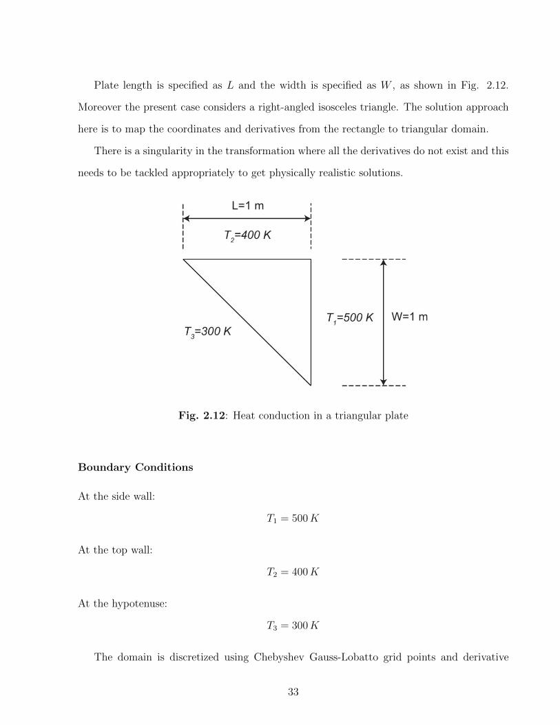
Plate length is specified as L and the width is specified as W , as shown in Fig. 2.12.
Moreover the present case considers a right-angled isosceles triangle. The solution approach
here is to map the coordinates and derivatives from the rectangle to triangular domain.
There is a singularity in the transformation where all the derivatives do not exist and this
needs to be tackled appropriately to get physically realistic solutions.
Fig. 2.12: Heat conduction in a triangular plate
Boundary Conditions
At the side wall:
T1 = 500K
At the top wall:
T2 = 400K
At the hypotenuse:
T3 = 300K
The domain is discretized using Chebyshev Gauss-Lobatto grid points and derivative
33

matrices are obtained by expressing the solution in terms of Chebyshev polynomials. A grid
size of 30×30 is used in the analysis and is found to be sufficient considering the high accuracy
and global nature of spectral methods. The horizontal side at y = −1 in the computational
domain is the source of singularity in the derivatives and so we tackled this issue by assigning
all the values at this y-level in the derivative matrices to zero.
2.6.2 Results
The isotherms were plotted for this problem and compared with a heat conduction problem
solution from the commercial solver ANSYS, as shown in Fig. 2.13. Contours are compared
and so this is a qualitative test but is rendered sufficient for bolstering credibility.
(a) Chebyshev collocation result (b) ANSYS result
Fig. 2.13: Isotherms for the triangular plate
The ANSYS model had roughly 20, 000 elements and the upper and right side walls were
partitioned into 200 equal sections. The left wall was divided into 283 elements so as to
maintain equal element length across the boundaries. Finally, a global element sizing of
5× 10⁻³ was enforced to get sufficient refinement near the center of the domain.
Through this problem we can conclude that simple diffusive terms can be handled properly.
34

Chapter 3
Parallelization of FDM Codes
3.1 1D Heat Conduction
Here we consider 1D heat conduction and use different methods to solve the same numerically.
For static heat conduction,
∂2T
∂x2= S (3.1)
We will discuss some methods to solve 1D-conduction problems with varying number of
points using different methods. We have considered the physical system depicted in fig. 3.1
with boundary conditions as Tleft = 300K and Tright = 400K
Fig. 3.1: 1D Heat conduction
Equation 3.1 is discretized using finite difference method to obtain a system of linear equations,
solution of which gives the temperature distribution along the discrete points considered.
aiTi = biTi+1 + ciTi−1 + di where i = 1, 2, 3, ...., N (3.2)
35

To account for the boundary points,
c1 = 0 and bN = 0 (3.3)
3.1.1 Jacobi Iterative Method
Jacobi method is an iterative method to solve a system of linear equations (Ax = b) which
starts with some initial guess. The result x at an iteration k is evaluated using the following
approach,
σi =n∑
j=1, j 6=i
aijx(k)j where i = 1, 2, 3, ...., N (3.4)
x(k+1)i =
1
aii(bi − σi) where i = 1, 2, 3, ...., N (3.5)
For the purpose of parallelization we have computed for different xi in parallel during each
iteration. Each processor is assigned a block of rows (xi) dynamically using the
!$OMP DO SCHEDULE(dynamic, [chunk size]) constuct.
No. of points Serial executionClock time (s)
Parallelexecution Clock
time (s)
Observedspeed-up
100 0.7445 0.2052 3.6281200 10.4809 2.7152 3.8601
Table 3.1: Jacobi iterative method
The table 3.1 shows that the observed speed - up of the parallel code against the serial
code is around 3.6 to 3.8. We used a quad - core CPU so the ideal speed-up is limited to 4.
3.1.2 Domain Decomposition in Space
In spatial domain decomposition method the physical domain is divided into a number of
sub-domains. We will use Tri-Diagonal Matrix Algorithm (TDMA)to solve each sub-domain
individually. In parallel version each domain is solved by a different core. Initially we
implemented for two sub-domains which was later extended to N domains. An initial guess
36

Fig. 3.2: Temperature distribution using Jacobi method
is made for the interface temperature and heat flux which serves as the boundary conditions
for the sub-domains. We then solve the two sub-domains in an iterative process. At the
interface of two sub-domains,
Ti, left =Ti, left + Ti, right
2(3.6)
Qi, right =Qi, left +Qi, right
2(3.7)
We use the following termination conditions,
|Qi, left −Qi, right| < ε1 and |Ti, left − Ti, right| < ε2 (3.8)
No. of points Iterationsrequired
Serialexecution
Clock time (s)
Parallelexecution
Clock time (s)
Observedspeed-up
1000 32 4.65616E-3 2.53811E-3 1.83452000 35 1.11364E-2 5.97120E-3 1.8650
Table 3.2: Domain decomposition with two subdomains
Table 3.2 shows the results for domain decomposition using two sub-domains. We can
37

see that the observed speed-up is close 2. Here we are restricted to use only two cores for the
parallel code as we are limiting to use only two sub-domains.
No. of points Iterationsrequired
Serialexecution
Clock time (s)
Parallelexecution
Clock time (s)
Observedspeed-up
1000 153 9.22481E-3 2.82501E-3 3.26542000 158 1.74712E-2 5.10879E-3 3.4112
Table 3.3: Domain decomposition with four subdomains
Table 3.3 shows the results for domain decomposition using four sub-domains. Though
we can see a speed-up of about 3.2 to 3.4 however, the execution time for the serial code with
four sub-domains is actually more than that for two sub-domains (comparing to results of
table 3.2). The execution time for parallel version of code with four sub-domains is slighlty
less than that for two sub-domains. We can also notice that the number iterations required
have increased. This can be explained by looking at how the information travels from the
left end to the right end. With four sub-domains we have three interfaces which obstruct the
flow of information in a single go. But as we solve the sub-domains parallely the execution
time is slightly less.
This may give a notion that domain decomposition isn’t a useful method. But we should
note that we have taken the initial guess at interface as random, which can be improved if
we first use a coarse mesh to get initial guesses.
In this chapter we provided details of the Jacobi iterative method and Domain decomposition
method which we have used to solve the 1D heat conduction problems using parallel computing.
We can see that the domain decomposition method using TDMA is much faster than Jacobi
iterative method. We also saw that for domain decomposition method as the number of
sub-domains increased the execution time increased as our initial guesses were random.
38

Fig. 3.3: Temperature distribution using domain decomposition
3.2 2D Heat Conduction
Here we consider 2D heat conduction and use different numerical methods to solve the
same with varying grid size. For a 2-D domain with uniform conductivity, the static heat
conduction equation,
∂2T
∂x2+∂2T
∂y2= S (3.9)
We have considered the physical system depicted in fig. 3.4 with boundary conditions as
Tbottom = 300 K and T = 400K on other three sides. Equation 3.9 is discretized using
finite difference method to obtain a system of linear equations, solution of which gives the
temperature distribution along the discrete points considered.
Using finite difference discretization,
2(1 + h2)TP = TEast + TWest + h2(TNorth + TSouth)− S∆x2 (3.10)
where, h = ∆x∆y
39

Fig. 3.4: 2D Heat conduction
3.2.1 TDMA Sweeps
TDMA Sweeps is line-by-line method to solve 2-D and 3-D systems which combines Gauss-Seidel
and TDMA methods. The grid points along a line are solved iteratively using TDMA. The
other terms are treated as constant for solving the grid points along the chosen line as shown
in fig. 3.5.
Fig. 3.5: TDMA line-by-line method [Patankar [1]]
The region is sweeped line-by-line in two directions using TDMA alternatively, first in
40

horizontal direction then in vertical direction. We have used the following condition for
termination incorporating l2 norm given as,
||X −Xprev||2 < ε (3.11)
Grid size Serial executionClock time (s)
Parallelexecution Clock
time (s)
Observedspeed-up
100 x 100 1.4427 0.6469 2.230200 x 200 19.9946 8.4437 2.368
Table 3.4: TDMA sweeps method
Table 3.4 shows the results for TDMA sweeps for 2-D heat conduction. The observed
speed - up is around 2.3 even though we used four processors. This could be due to the
overhead of calculating the norm of X −Xprev at each iteration.
Fig. 3.6: Temperature distribution using TDMA sweeps
41

3.2.2 Domain Decomposition with Two Sub-Domains
Similar to 1-D domain decomposition the domain is divided into multiple sub-domains, the
only difference being the sub-domains are rectangular. TDMA sweeps has been used to solve
each rectangular sub-domain. Similar to 1D domain decoposition each domain is solved
by a different core concurrently in the parallel version of the code. For now it has been
implemented for two subdomains which will be extended to N domains later. At the interface
of two sub-domains,
TiNx1,left =TiNx1,left + Ti1,right
2where i = 1, 2, ...., Ny (3.12)
Qi1,right =QiNx1,left +Qi1,right
2where i = 1, 2, ...., Ny (3.13)
Grid size Iterationsrequired
Serialexecution
Clock time(s)
Parallelexecution
Clock time(s)
Observedspeed-up
100 x 100 5 7.74840 5.03571 1.5386200 x 200 6 98.70741 62.33654 1.5835
Table 3.5: 2D domain decomposition with two sub-domains
Table 3.5 shows the results for 2-D domain decomposition using two sub-domains. Though
we can see a speed-up of about 1.5 to 1.6 however, the execution time for code with two
sub-domains is actually more than that for TDMA Sweeps (comparing to results of table
3.4). It should also be noted that the number of iterations of TDMA sweeps for domain
decomposition is 5-6 whereas if we use TDMA sweeps alone only one iteration of TDMA
sweeps is required.
This can explained by looking at how the information travels from left end to the right
end in domain decomposition. Similar to 1-D the interface of two sub-domains obstructs the
flow of information in a single go. As in 1-D the initial guess for temperature and heat flux is
taken to be random which can be improved by using results of coarse mesh as initial guess.
42

Fig. 3.7: Temperature distribution using domain decomposition
TDMA sweeps was found to be better as with domain decomposition method the interface
obstructs the flow of information. While using a uniform mesh we find TDMA sweeps to
be of more use however, to solve non-uniform mesh domain decomposition will be greater
use. Domain decomposition can further be improved by using coarse mesh to get the initial
guesses.
43


Chapter 4
Parallelization of Spectral Codes
Spectral methods use a predefined Chebyshev grid for the given number of elements and
computational domain. The Chebyshev grid is characteristically fine at the corners but
relatively coarser in the mid-section of the domain. As a result, in problems involving
resolution of flow phenomena near the center of the domain we must resort to higher number
of elements. Moreover, spectral methods exhibit consistent accuracy above a threshold
grid size implying that further refinements would increase computations without improving
accuracy. Thus partitioning the domain and solving each of them using spectral method
would result in refinements within the domain.
4.1 One Dimensional Heat Conduction
In this section we solve the simplest problem of one-dimensional heat conduction to develop
the framework for domain decomposition in spectral methods.
4.1.1 Physical System
The physical model can be thought to be a slender rod with sides maintained at constant
but different temperatures. This slender assumption retains the one-dimensional nature of
the problem.
45
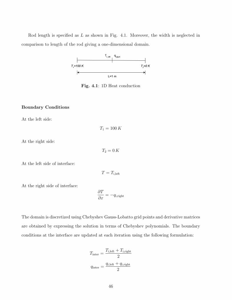
Rod length is specified as L as shown in Fig. 4.1. Moreover, the width is neglected in
comparison to length of the rod giving a one-dimensional domain.
Fig. 4.1: 1D Heat conduction
Boundary Conditions
At the left side:
T1 = 100K
At the right side:
T2 = 0K
At the left side of interface:
T = Ti,left
At the right side of interface:
∂T
∂x= −qi,right
The domain is discretized using Chebyshev Gauss-Lobatto grid points and derivative matrices
are obtained by expressing the solution in terms of Chebyshev polynomials. The boundary
conditions at the interface are updated at each iteration using the following formulation:
Tinter =Ti,left + Ti,right
2
qinter =qi,left + qi,right
2
46
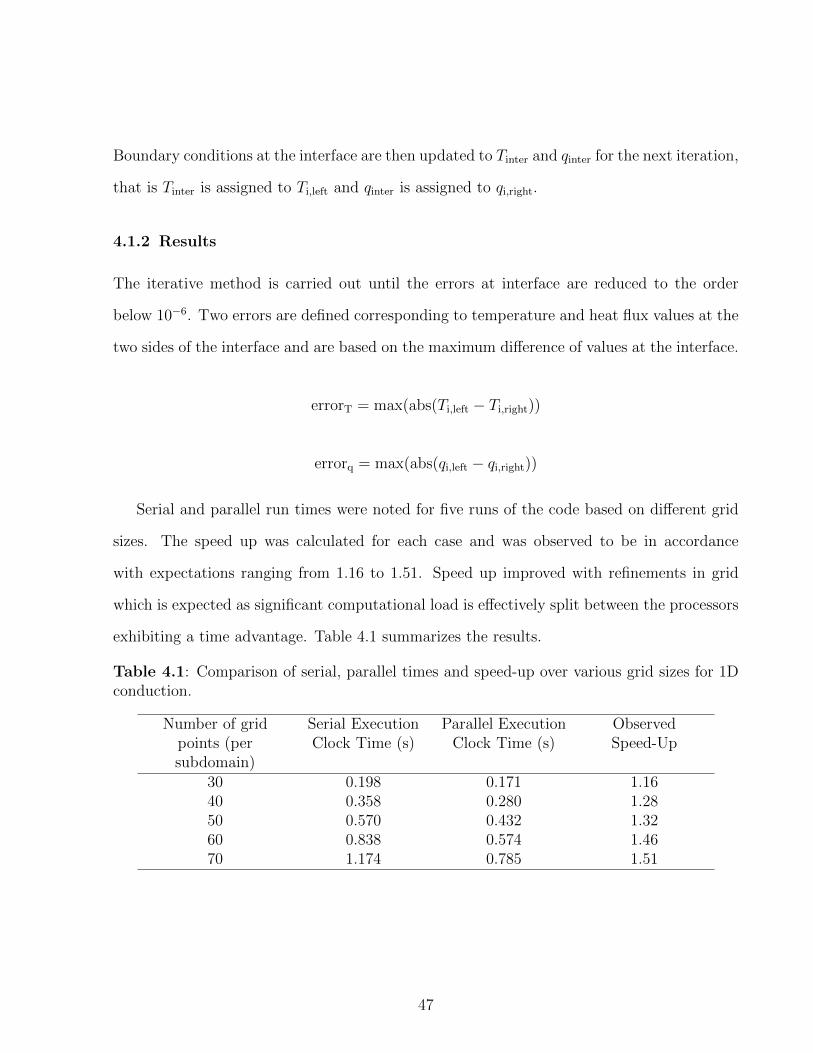
Boundary conditions at the interface are then updated to Tinter and qinter for the next iteration,
that is Tinter is assigned to Ti,left and qinter is assigned to qi,right.
4.1.2 Results
The iterative method is carried out until the errors at interface are reduced to the order
below 10−6. Two errors are defined corresponding to temperature and heat flux values at the
two sides of the interface and are based on the maximum difference of values at the interface.
errorT = max(abs(Ti,left − Ti,right))
errorq = max(abs(qi,left − qi,right))
Serial and parallel run times were noted for five runs of the code based on different grid
sizes. The speed up was calculated for each case and was observed to be in accordance
with expectations ranging from 1.16 to 1.51. Speed up improved with refinements in grid
which is expected as significant computational load is effectively split between the processors
exhibiting a time advantage. Table 4.1 summarizes the results.
Table 4.1: Comparison of serial, parallel times and speed-up over various grid sizes for 1Dconduction.
Number of gridpoints (persubdomain)
Serial ExecutionClock Time (s)
Parallel ExecutionClock Time (s)
ObservedSpeed-Up
30 0.198 0.171 1.1640 0.358 0.280 1.2850 0.570 0.432 1.3260 0.838 0.574 1.4670 1.174 0.785 1.51
47

4.2 Two Dimensional Heat Conduction
4.2.1 Domain Decomposition with Two Subdomains
In this problem we extend our knowledge of domain decomposition in one-dimensional
problems to two-dimensional ones. This section deals with dividing the domain into two
parts and solving them individually using spectral method.
Physical System
The physical model consists of a rectangular plate with sides maintained at constant but
different temperatures. A partition is made at the center of the plate in the computational
domain but the final solution is reflected as a whole.
Plate length is specified as L and the width is specified as W , as shown in Fig. 4.2.
Moreover the partition is made at length 0.5L giving us two sub-domains each of length 0.5L
and width W .
Fig. 4.2: 2D Heat conduction - two subdomains
Boundary Conditions
At the top wall:
Th = 400K
48

At the left, right and bottom wall:
Tc = 300K
At the left side of interface:
T = Ti,left
At the right side of interface:
∂T
∂x= −qi,right
The domain is discretized using Chebyshev Gauss-Lobatto grid points and derivative matrices
are obtained by expressing the solution in terms of Chebyshev polynomials. Similar to the
one-dimensional case, boundary conditions at the interface are updated at each iteration
using the following formulation:
Tinter =Ti,left + Ti,right
2
qinter =qi,left + qi,right
2
Boundary conditions at the interface are then updated to Tinter and qinter for the next iteration,
that is Tinter is assigned to Ti,left and qinter is assigned to qi,right.
Results
The iterative method is carried out until the errors at interface are reduced to the order
below 10−6. Two errors are defined corresponding to temperature and heat flux values at the
two sides of the interface and are based on the maximum difference of values at the interface.
errorT = max(abs(Ti,left − Ti,right))
errorq = max(abs(qi,left − qi,right))
49

Comparing the numerical solution with analytical result we observe that they coincide exactly
thereby verifying spectral accuracy. Also, refinements near the center can be observed in plot
4.3 with concentrated points at the corners and center.
Fig. 4.3: Midline profile comparison
Solutions from both the domains were combined finally to constitute an overall temperature
field. Thereafter, a temperature contour plot shown in Fig 4.4 helped in assuring continuity
among the results from the left and right sub-domains.
Serial and parallel run times were noted for five runs of the code based on different grid
sizes. The speed up was calculated for each case and was observed to be in accordance
with expectations ranging from 1.38 to 1.89. Speed up improved with refinements in grid
which is expected as significant computational load is effectively split between the processors
exhibiting a time advantage. Table 4.2 summarizes the results.
50

Fig. 4.4: Temperature contour plot for two subdomains
Table 4.2: Comparison of serial, parallel times and speed-up over various grid sizes for 2Dconduction with two subdomains.
Number of gridpoints (persubdomain)
Serial ExecutionClock Time (s)
Parallel ExecutionClock Time (s)
ObservedSpeed-Up
20× 20 1.027 0.746 1.3830× 30 9.693 5.584 1.7435× 35 23.635 12.910 1.8340× 40 51.222 27.329 1.8850× 50 190.84 101.24 1.89
4.2.2 Domain Decomposition with Four Subdomains
This section extends over the previous case and deals with dividing the domain into four
parts, solving them individually. This formulation serves crucial for extending the algorithm
to domain decomposition involving multiple sub-domains.
51

Physical System
The physical model consists of a rectangular plate with sides maintained at constant but
different temperatures. Partition are made at the center of the plate in the computational
domain but the final solution is reflected as a whole.
Plate length is specified as L and the width is specified as W , as shown in Fig. 4.5.
Moreover partitions are made at length 0.5L and width 0.5L, giving us four sub-domains
each of length 0.5L and width 0.5W .
Fig. 4.5: 2D Heat conduction - four subdomains
Boundary Conditions
At the top wall:
Th = 400K
At the left, right and bottom wall:
Tc = 300K
Interface boundary conditions are critical for this problem because it was observed that
52

having two Neumann boundary conditions in a domain leads to divergence. These boundary
conditions are initially random guesses which are updated every iteration to finally give a
physically realistic result. So the interface conditions follow the pattern given in fig 4.5
The domain is discretized using Chebyshev Gauss-Lobatto grid points and derivative
matrices are obtained by expressing the solution in terms of Chebyshev polynomials. Similar
to the one-dimensional case, boundary conditions at the interface are updated at each
iteration using the following formulation:
Tinter =Ti,left + Ti,right
2
qinter =qi,left + qi,right
2
Boundary conditions at the interface are then updated to Tinter and qinter for the next iteration,
that is Tinter is assigned to Ti,left and qinter is assigned to qi,right.
Results
The iterative method is carried out until the errors at interface are reduced to the order
below 10−6. Two errors are defined corresponding to temperature and heat flux values at the
two sides of the interface and are based on the maximum difference of values at the interface.
errorT = max(abs(Ti,left − Ti,right))
errorq = max(abs(qi,left − qi,right))
Comparing the numerical solution with analytical result we observe that they coincide exactly
thereby verifying spectral accuracy. For this problem we have two mid-lines and the values
of temperature are compared along these as shown in Fig. 4.6 and Fig. 4.7. In addition,
refinements at the center of the domain can be observed by the clustering of points near the
corners and mid-portion of the plots.
53

Fig. 4.6: Vertical midline profile comparison
Fig. 4.7: Horizontal midline profile comparison
54

Solutions from all four domains were combined finally to constitute an overall temperature
field. Thereafter, a temperature contour plot shown in Fig 4.8 helped in assuring continuity
among the results from the four sub-domains together.
Fig. 4.8: Temperature contour plot for four subdomains
Serial and parallel run times were noted for five runs of the code based on different grid
sizes. The speed up was calculated for each case and was observed to be in accordance
with expectations ranging from 2.43 to 2.71. Speed up improved with refinements in grid
which is expected as significant computational load is effectively split between the processors
exhibiting a time advantage. Table 4.3 summarizes the results.
Table 4.3: Comparison of serial, parallel times and speed-up over various grid sizes for 2Dconduction with four subdomains.
Number of gridpoints (persubdomain)
Serial ExecutionClock Time (s)
Parallel ExecutionClock Time (s)
ObservedSpeed-Up
20× 20 6.76 2.782 2.4330× 30 54.964 21.811 2.5235× 35 120.47 46.694 2.5840× 40 235.43 89.178 2.6450× 50 746.68 275.528 2.71
55
4.3 Channel Flow
4.3.1 Domain Decomposition with Two Subdomains
This section extends the algorithm of domain decomposition in spectral methods to fluid
flow problems. Previous problems established the method for elliptic equations covered
predominantly using heat conduction. Current section deals with a simple problem involving
fully developed flow between two parallel plates.
Physical System
The physical model consists of a fully developed flow between two infinite parallel plates
separated by a unit distance. Flow is assumed to be fully developed at the inlet and gradients
along streamwise directions are set to zero for velocity and pressure at the outlet. The top
and bottom walls have a no-slip boundary condition for velocity and zero normal pressure
gradients.
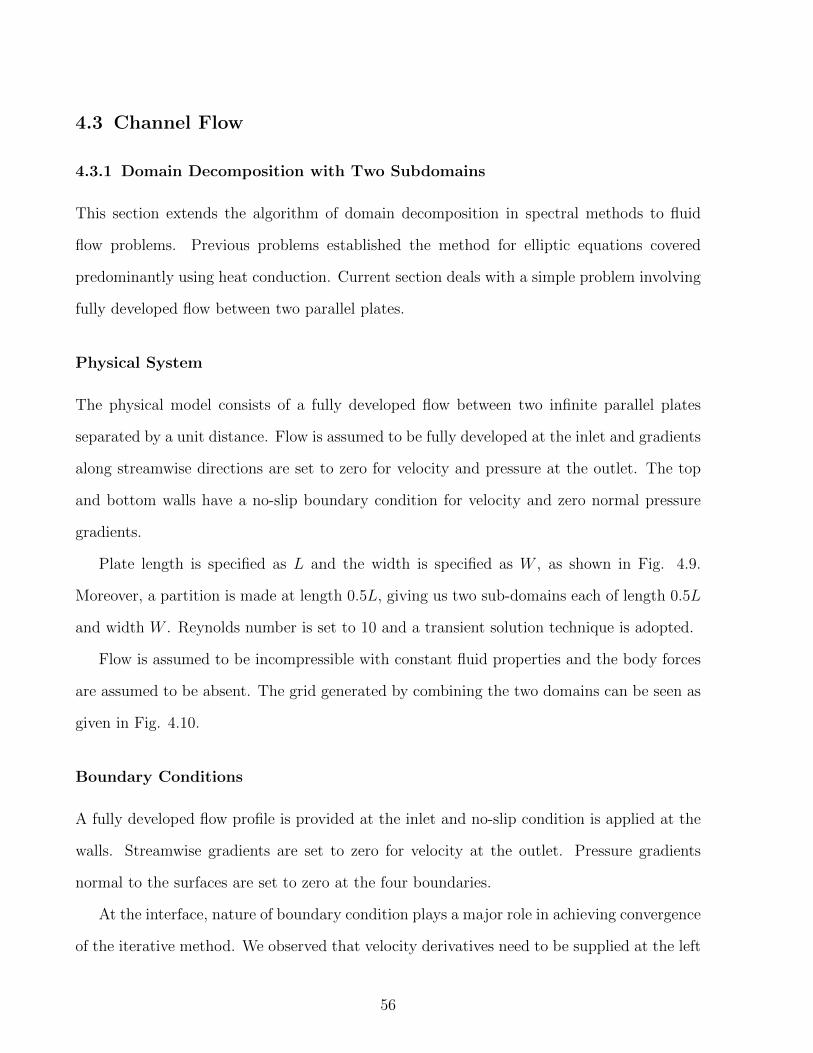
Plate length is specified as L and the width is specified as W , as shown in Fig. 4.9.
Moreover, a partition is made at length 0.5L, giving us two sub-domains each of length 0.5L
and width W . Reynolds number is set to 10 and a transient solution technique is adopted.
Flow is assumed to be incompressible with constant fluid properties and the body forces
are assumed to be absent. The grid generated by combining the two domains can be seen as
given in Fig. 4.10.
Boundary Conditions
A fully developed flow profile is provided at the inlet and no-slip condition is applied at the
walls. Streamwise gradients are set to zero for velocity at the outlet. Pressure gradients
normal to the surfaces are set to zero at the four boundaries.
At the interface, nature of boundary condition plays a major role in achieving convergence
of the iterative method. We observed that velocity derivatives need to be supplied at the left
56

Fig. 4.9: Channel flow - two subdomains
Fig. 4.10: Combined grid layout for two subdomains
interface and pressure derivatives at the right interface.
At the top and bottom wall:
u = 0, v = 0,∂p
∂y= 0
57

At the inlet:
u = 1− y2, v = 0,∂p
∂x= 0
At the outlet:
∂u
∂x= 0,
∂v
∂x= 0,
∂p
∂x= 0
At the left interface:
∂u
∂x=∂u
∂x i,
∂v
∂x=∂v
∂x i, p = pi
At the right interface:
u = ui, v = vi,∂p
∂x=∂p
∂x i
Interface values for primitive variables are updated after each iteration in the same way
as represented in the conduction problems involving Ti and qi.
Results
The iterative method is carried out until the errors at interface are reduced to the order
below 10−6. Two errors are defined each for u, v velocity components and pressure at the
two sides of the interface, similar to temperature and heat flux errors defined in conduction
problems.
Solutions from both the domains were combined finally to constitute an overall field for
velocity components and pressure. Thereafter, a velocity vector plot given by Fig.4.11 helped
in ensuring function continuity at the interface and providing a qualitative idea of solution
accuracy.
Serial and parallel run times were noted for five runs of the code based on different grid
sizes. The speed up was calculated for each case and was observed to be in accordance
with expectations ranging from 1.65 to 1.79. Speed up improved with refinements in grid
which is expected as significant computational load is effectively split between the processors
exhibiting a time advantage. Table 4.4 summarizes the results.
58

Fig. 4.11: Velocity vectors for channel flow with two subdomains
Table 4.4: Comparison of serial, parallel times and speed-up over various grid sizes forchannel flow with two subdomains.
Number of gridpoints (persubdomain)
Serial ExecutionClock Time (s)
Parallel ExecutionClock Time (s)
ObservedSpeed-Up
10× 20 13.555 8.215 1.6515× 30 78.734 46.865 1.6820× 40 271.54 157.87 1.7230× 30 345.53 198.58 1.7425× 50 694.41 387.94 1.79
4.3.2 Domain Decomposition with Four Subdomains
This problem considers a two-dimensional channel flow between infinite parallel plates with
four sub-domains. Current formulation serves as a foundation for observing the behaviour of
our algorithm in the presence of multiple sub-domains.
59

Physical System
The physical model consists of a fully developed flow between two infinite parallel plates
separated by a unit distance. Flow is assumed to be fully developed at the inlet and gradients
along streamwise directions are set to zero for velocity and pressure at the outlet. The top
and bottom walls have a no-slip boundary condition for velocity and zero normal pressure
gradients.
Plate length is specified as L and the width is specified as W , as shown in Fig. 4.12.
Moreover, partitions are made at length 0.5L and width 0.5W , giving us four sub-domains
each of length 0.5L and width 0.5W . Reynolds number is set to 10 and a transient solution
technique is adopted.
Flow is assumed to be incompressible with constant fluid properties and the body forces
are assumed to be absent. Only derivatives are represented using Du,v and Dp in Fig. 4.12 to
preserve clarity and other interface boundary conditions should be taken as value assignment
type. The grid generated by combining the four domains can be seen as given in Fig. 4.13.
Fig. 4.12: Channel flow - four subdomains
60

Fig. 4.13: Combined grid layout for four subdomains
Boundary Conditions
A fully developed flow profile is provided at the inlet and no-slip condition is applied at the
walls. Streamwise gradients are set to zero for velocity at the outlet. Pressure gradients
normal to the surfaces are set to zero at the four boundaries.
Building upon the previous problem, the interface boundary conditions play a cardinal
role in obtaining a correct solution. Fig. 4.12 shows the pattern in which boundary conditions
should be assigned extending from two subdomains.
At the top and bottom wall:
u = 0, v = 0,∂p
∂y= 0
At the inlet:
u = 1− y2, v = 0,∂p
∂x= 0
61

At the outlet:
∂u
∂x= 0,
∂v
∂x= 0,
∂p
∂x= 0
The interface boundary conditions are shown in Fig. 4.12. Interface values for primitive
variables are updated after each iteration in the same way as represented in the conduction
problems involving Ti and qi.
Results
The iterative method is carried out until the errors at interface are reduced to the order
below 10−6. Two errors are defined each for u, v velocity components and pressure at the
two sides of the interface, similar to temperature and heat flux errors defined in conduction
problems.
Solutions from all four domains were combined finally to constitute an overall field for
velocity components and pressure. Thereafter, a velocity vector plot given by Fig.4.14 helped
in ensuring function continuity at the interface and providing a qualitative idea of solution
accuracy.
Serial and parallel run times were noted for five runs of the code based on different grid
sizes. The speed up was calculated for each case and was observed to be in accordance
with expectations ranging from 2.36 to 2.83. Speed up improved with refinements in grid
which is expected as significant computational load is effectively split between the processors
exhibiting a time advantage. Table 4.5 summarizes the results.
62

Fig. 4.14: Velocity vectors for channel flow with four subdomains
Table 4.5: Comparison of serial, parallel times and speed-up over various grid sizes forchannel flow with four subdomains.
Number of gridpoints (persubdomain)
Serial ExecutionClock Time (s)
Parallel ExecutionClock Time (s)
ObservedSpeed-Up
10× 10 13.197 5.5919 2.3615× 15 79.347 31.487 2.5220× 20 255.39 96.739 2.6425× 25 664.85 241.76 2.7530× 30 1438.6 508.34 2.83
63

4.4 Lid Driven Cavity
4.4.1 Domain Decomposition with Two Subdomains
This section considers a slightly advanced fluid flow problem for realizing internal recirculating
flows within a bounded domain. The model physically represents a square cavity with a
driven lid to induce recirculation. Computational space is divided into two subdomains, each
of which is solved using spectral method exchanging information at the interface.
Physical System
A square enclosure with driven lid on its top surface is taken as the physical model,as shown in
Fig. 4.15. No-slip boundary condition is applied at the walls barring the lid which is driven
with a profile consistent with zero velocity at the edges. Normal to the surface pressure
gradients are set to zero.
Enclosure length is specified as L and the width is specified as W , as shown in Fig. 4.15.
Moreover, a partition is made at length 0.5L, giving us two sub-domains each of length 0.5L
and width W .
Flow is assumed to be incompressible with constant fluid properties and the body forces
are assumed to be absent.
Boundary Conditions
No-slip boundary condition is enforced over all the walls except the lid which is driven at
a velocity conformal to zero value at the edges. Pressure gradients normal to the boundary
surfaces are set to zero and in addition pressure value at the center of the cavity is taken to
be zero.
Building upon the previous problem, the interface boundary conditions play a cardinal
role in obtaining a correct solution. The resulting boundary conditions can be mathematically
given as,
64

Fig. 4.15: Lid driven cavity - two subdomains
At the left and right wall:
u = 0, v = 0,∂p
∂x= 0
At the bottom wall:
u = 0, v = 0,∂p
∂y= 0
At the lid:
u = 16x2(1− x2), v = 0,∂p
∂y= 0
At the domain’s center point:
p = 0
At the left interface:
∂u
∂x=∂u
∂x i,
∂v
∂x=∂v
∂x i, p = pi
65

At the right interface:
u = ui, v = vi,∂p
∂x=∂p
∂x i
Interface values for primitive variables are updated after each iteration in the same way as
represented in the conduction problems involving Ti and qi.
Results
The iterative method is carried out until the errors at interface are reduced to the order
below 10−6. Two errors are defined each for u, v velocity components and pressure at the
two sides of the interface, similar to temperature and heat flux errors defined in conduction
problems.
Solutions from both the domains were combined finally to constitute an overall field for
velocity components and pressure. Thereafter, a velocity vector plot given by Fig.4.16 helped
in ensuring function continuity at the interface and providing a qualitative idea of solution
accuracy.
Serial and parallel run times were noted for five runs of the code based on different grid
sizes. The speed up was calculated for each case and was observed to be in accordance
with expectations ranging from 1.78 to 1.91. Speed up improved with refinements in grid
which is expected as significant computational load is effectively split between the processors
exhibiting a time advantage. Table 4.6 summarizes the results.
Table 4.6: Comparison of serial, parallel times and speed-up over various grid sizes for liddriven cavity with two subdomains.
Number of gridpoints (persubdomain)
Serial ExecutionClock Time (s)
Parallel ExecutionClock Time (s)
ObservedSpeed-Up
10× 20 38.855 21.829 1.7815× 30 218.81 120.23 1.8220× 40 730.47 392.73 1.8630× 30 931.45 492.83 1.8925× 50 1858.7 973.14 1.91
66

Fig. 4.16: Velocity vectors for lid driven flow at Re = 10
4.4.2 Domain Decomposition with Four Subdomains
This section extends the previous problem dividing the computational domain into four
subdomains. Each of the subdomains share information at their interfaces and this problem
examines the characteristics of our algorithm with multiple subdomains.
Physical System
A square enclosure with driven lid on its top surface is taken as the physical model,as shown in
Fig. 4.17. No-slip boundary condition is applied at the walls barring the lid which is driven
with a profile consistent with zero velocity at the edges. Normal to the surface pressure
gradients are set to zero.
Enclosure length is specified as L and the width is specified as W , as shown in Fig. 4.15.
Moreover, partitions are made at length 0.5L and width 0.5W , giving four sub-domains each
of length 0.5L and width 0.5W .
67

Flow is assumed to be incompressible with constant fluid properties and the body forces
are assumed to be absent.
Fig. 4.17: Lid driven cavity - four subdomains
Boundary Conditions
No-slip boundary condition is enforced over all the walls except the lid which is driven at
a velocity conformal to zero value at the edges. Pressure gradients normal to the boundary
surfaces are set to zero and in addition pressure value at the center of the cavity is taken to
be zero.
Building upon the previous problem, the interface boundary conditions play a cardinal
role in obtaining a correct solution. Fig. 4.17 shows the pattern in which boundary conditions
should be assigned extending from two subdomains. The resulting boundary conditions can
be mathematically given as,
68

At the left and right wall:
u = 0, v = 0,∂p
∂x= 0
At the bottom wall:
u = 0, v = 0,∂p
∂y= 0
At the lid:
u = 16x2(1− x2), v = 0,∂p
∂y= 0
At the domain’s center point:
p = 0
The interface boundary conditions are shown in Fig. 4.17. Interface values for primitive
variables are updated after each iteration in the same way as represented in the conduction
problems involving Ti and qi.
Results
The iterative method is carried out until the errors at interface are reduced to the order
below 10−6. Two errors are defined each for u, v velocity components and pressure at the
two sides of the interface, similar to temperature and heat flux errors defined in conduction
problems.
Serial and parallel run times were noted for five runs of the code based on different grid
sizes. The speed up was calculated for each case and was observed to be in accordance
with expectations ranging from 2.57 to 2.87. Speed up improved with refinements in grid
which is expected as significant computational load is effectively split between the processors
exhibiting a time advantage. Table 4.7 summarizes the results.
69

Table 4.7: Comparison of serial, parallel times and speed-up over various grid sizes for liddriven cavity with four subdomains.
Number of gridpoints (persubdomain)
Serial ExecutionClock Time (s)
Parallel ExecutionClock Time (s)
ObservedSpeed-Up
10× 10 33.836 13.924 2.4315× 15 209.54 83.151 2.5220× 20 733.16 284.17 2.5825× 25 1786.4 676.67 2.6430× 30 4020.7 1483.7 2.71
70

Chapter 5
Conclusions
In this work, CFD solver for the computation of incompressible heat transfer and fluid flows
is developed. The solver for incompressible heat transfer and fluid flows is based on spectral
method. The parallelization of these codes is based on the domain decomposition method
using OpenMP.
For incompressible flows:
1. Heat conduction in rectangular domains has been verified with analytical solutions and
can be concluded to be coherent with the same.
2. Results for the Lid-driven cavity are in strong agreement with benchmarks and the
maximum percentage error is found to be less than 2%
3. Natural convection results of streamfunction contours and isotherms are found to be
matching high-accuracy solutions prevalent in literature.
4. Heat conduction in triangular domain has been successfully verified with results from
ANSYS and so the code can be asserted as applicable to non-rectangular domains for
conduction problems.
In conclusion these problems helped establish our algorithm as general for incompressible
fluid flow and heat transfer problems.
71

For parallelization:
1. One dimensional and Two dimensional heat conduction codes formulated using FDM
were successfully parallelized using two and four subdomains.
2. Parallelization of Spectral codes for conduction was carried out using 1D and 2D
problems using two and four subdomains with speed up ranging from 1.69 to 2.73.
3. Finally the algorithm for domain decomposition was extended to solve fluid flow cases
using channel flow and lid driven cavity problems with speed up ranging from 1.74 to
2.91.
In conclusion, the algorithm of domain decomposition for parallelization was deemed to be
working for conduction and simple fluid flow problems using both spectral methods and FDM
for discretization.
5.1 Future Scope
The present work has the following potential future scope:
1. Heat and fluid flow problems can be handled in irregular domains using spectral
methods by incorporating appropriate grid transformation techniques.
2. Refining the domain decomposition codes for fluid flow problems to attain better
speed-up and to solve high Reynolds number situations.
3. Extending domain decomposition method to heat flow problems based on the foundations
of fluid flow algorithms.
4. Handling conduction problems in irregular geometries using the domain decomposition
algorithm developed for regular domains and a suitable transformation.
72

References
[1] Suhas V. Patankar. Numerical Heat Transfer and Fluid Flow. CRC Press, Taylor &
Francis Group, 2009.
[2] Llyod N. Trefethen. Spectral Methods in Matlab. Society for Industrial and Applied
Mathematics (SIAM).
[3] P. R. Spalart, R. D. Moser and M. M. Rogers. Spectral Methods for the Navier-Stokes
Equations with One Infinite and Two Periodic Directions. Journal of Computational
Physics, 1991, 297-324.
[4] C. Canuto, M. Y. Hussaini, A. Quarteroni and T. A. Zang. Spectral Methods in Fluid
Dynamics. Springer-Verlag, Berlin, 1987.
[5] D. Gottlieb and S. A. Orszag. Numerical Analysis of Spectral Methods. SIAM,
Philadelphia, 1977.
[6] A. Solomonoff and E. Turkel. Global Properties of Pseudospectral Methods. Computational
Physics, Vol. 81, 1989, 239-276.
[7] M. Deville, P. F. Fischer and E. H. Mund. High-Order Methods for Incompressible Fluid
Flow. Cambridge Monographs on Applied and Computational Mathematics. Cambridge
University Press, 2002.
[8] O. Botella. On the Solution of Navier-Stokes Equations using Chebyshev Projection
Schemes with Third-Order accuracy in Time. Computers & Fluids, Vol. 26, 1997, 107-116.
73

[9] A. J. Chorin. Numerical Solution of the Navier-Stokes Equations. Mathematics of
Computation, Vol. 22, 1968, 745-762.
[10] R. Temam. Une Mthode dApproximation de la Solution des quations de Navier-Stokes.
Bulletin of Society Mathematics of France, Vol. 98, 1968, 115-152.
[11] S. Huges and A. Randriamampianina. An Improved Projection Scheme Applied to
Pseudospectral Methods for the Incompressible Navier-Stokes Equations. International
Journal for Numerical Methods in Fluids, Vol. 28, 1998, 501-521.
[12] C. L. Streett and M. G. Macaraeg. Spectral Multi-Domain for Large-Scale Fluid Dynamic
Simulations. Applied Numerical Mathematics, Vol. 6, 1989/90, 123-139.
[13] William D. Gropp and David E. Keyes. Domain Decomposition Methods In
Computational Fluid Dynamics. International Journal For Numerical Methods In Fluids,
Vol. 14, 147-165, 1992.
[14] L.M.R. Carvalho and J.M.L.M. Palma. Parallelization of CFD Code Using PVM and
Domain Decomposition Techniques. International Conference on Vector and Parallel
Processing, 247-257, 1996.
[15] Maria Giuseppina Chiara Nestola, Barna Becsekb, Hadi Zolfagharib, Patrick Zuliana,
Dario De Marinisb, Rolf Krausea and Dominik Obristb. An immersed boundary method
for fluid-structure interaction based on overlapping domain decomposition. Journal of
Computational Physics , 2018.
[16] A. Jagannathan, R. Mohan and M. Dhanak. A spectral method for the triangular cavity
flow. Computers & Fluids, Vol. 95, 2014, 40-48.
[17] J. P. Holman. Heat Transfer. Mc-Graw Hill Higher Education, 1977.
74

[18] U. Ehrenstein and R. Peyret A Chebyshev Spectral Collocation Method for the
Navier-Stokes Equations with Application to Double-Diffusive Convection. International
Journal for Numerical Methods in Fluids, Vol. 9, 1989, 427-452.
[19] J. J. Martinez and P. T. Esperana. A Chebyshev collocation spectral method for numerical
simulation of incompressible flow problems. Journal of the Brazilian Society of Mechanical
Sciences and Engineering, 29(3), 2007, 317-328.
[20] T. Saitoh and K. Hirose. High-accuracy bench mark solutions to natural convection in a
square cavity. Computational Mechanics, Vol. 4, 1989, 417-427
[21] J. D. Anderson Jr. Computational Fluid Dynamics: The Basics with Applications.
McGraw-Hill, NewYork, 1995.
75