arX

iv:p

hysi

cs/0

2121

13 v

2 3

1 D

ec 2

002

Computation in a single neuron:

Hodgkin and Huxley revisited

Blaise Aguera y Arcas,1 Adrienne L. Fairhall,2,3 and William Bialek2,4

1Rare Books Library, Princeton University, Princeton, New Jersey 085442NEC Research Institute, 4 Independence Way, Princeton, New Jersey 085403Department of Molecular Biology, Princeton University, Princeton, New Jersey 085444Department of Physics, Princeton University, Princeton, New Jersey 08544

{blaisea,fairhall,wbialek}@princeton.edu

31 December 2002

A spiking neuron “computes” by transforming a complex dynamical input into a train of

action potentials, or spikes. The computation performed by the neuron can be formulated as

dimensional reduction, or feature detection, followed by a nonlinear decision function over the

low dimensional space. Generalizations of the reverse correlation technique with white noise

input provide a numerical strategy for extracting the relevant low dimensional features from

experimental data, and information theory can be used to evaluate the quality of the low–

dimensional approximation. We apply these methods to analyze the simplest biophysically

realistic model neuron, the Hodgkin–Huxley model, using this system to illustrate the general

methodological issues. We focus on the features in the stimulus that trigger a spike, explicitly

eliminating the effects of interactions between spikes. One can approximate this triggering

“feature space” as a two dimensional linear subspace in the high–dimensional space of input

histories, capturing in this way a substantial fraction of the mutual information between

inputs and spike time. We find that an even better approximation, however, is to describe

the relevant subspace as two dimensional, but curved; in this way we can capture 90% of the

mutual information even at high time resolution. Our analysis provides a new understanding

of the computational properties of the Hodgkin–Huxley model. While it is common to

approximate neural behavior as “integrate and fire,” the HH model is not an integrator nor

is it well described by a single threshold.

1

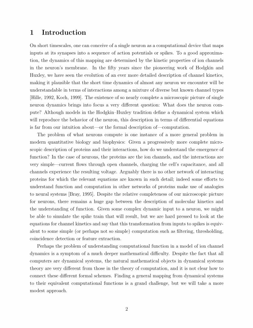
1 Introduction

On short timescales, one can conceive of a single neuron as a computational device that maps

inputs at its synapses into a sequence of action potentials or spikes. To a good approxima-

tion, the dynamics of this mapping are determined by the kinetic properties of ion channels

in the neuron’s membrane. In the fifty years since the pioneering work of Hodgkin and

Huxley, we have seen the evolution of an ever more detailed description of channel kinetics,

making it plausible that the short time dynamics of almost any neuron we encounter will be

understandable in terms of interactions among a mixture of diverse but known channel types

[Hille, 1992, Koch, 1999]. The existence of so nearly complete a microscopic picture of single

neuron dynamics brings into focus a very different question: What does the neuron com-

pute? Although models in the Hodgkin–Huxley tradition define a dynamical system which

will reproduce the behavior of the neuron, this description in terms of differential equations

is far from our intuition about—or the formal description of—computation.

The problem of what neurons compute is one instance of a more general problem in

modern quantitative biology and biophysics: Given a progressively more complete micro-

scopic description of proteins and their interactions, how do we understand the emergence of

function? In the case of neurons, the proteins are the ion channels, and the interactions are

very simple—current flows through open channels, charging the cell’s capacitance, and all

channels experience the resulting voltage. Arguably there is no other network of interacting

proteins for which the relevant equations are known in such detail; indeed some efforts to

understand function and computation in other networks of proteins make use of analogies

to neural systems [Bray, 1995]. Despite the relative completeness of our microscopic picture

for neurons, there remains a huge gap between the description of molecular kinetics and

the understanding of function. Given some complex dynamic input to a neuron, we might

be able to simulate the spike train that will result, but we are hard pressed to look at the

equations for channel kinetics and say that this transformation from inputs to spikes is equiv-

alent to some simple (or perhaps not so simple) computation such as filtering, thresholding,

coincidence detection or feature extraction.

Perhaps the problem of understanding computational function in a model of ion channel

dynamics is a symptom of a much deeper mathematical difficulty. Despite the fact that all

computers are dynamical systems, the natural mathematical objects in dynamical systems

theory are very different from those in the theory of computation, and it is not clear how to

connect these different formal schemes. Finding a general mapping from dynamical systems

to their equivalent computational functions is a grand challenge, but we will take a more

modest approach.

2

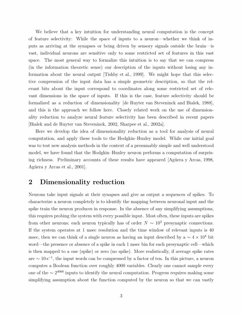
We believe that a key intuition for understanding neural computation is the concept

of feature selectivity: While the space of inputs to a neuron—whether we think of in-

puts as arriving at the synapses or being driven by sensory signals outside the brain—is

vast, individual neurons are sensitive only to some restricted set of features in this vast

space. The most general way to formalize this intuition is to say that we can compress

(in the information theoretic sense) our description of the inputs without losing any in-

formation about the neural output [Tishby et al., 1999]. We might hope that this selec-

tive compression of the input data has a simple geometric description, so that the rel-

evant bits about the input correspond to coordinates along some restricted set of rele-

vant dimensions in the space of inputs. If this is the case, feature selectivity should be

formalized as a reduction of dimensionality [de Ruyter van Steveninck and Bialek, 1988],

and this is the approach we follow here. Closely related work on the use of dimension-

ality reduction to analyze neural feature selectivity has been described in recent papers

[Bialek and de Ruyter van Steveninck, 2002, Sharpee et al., 2002a].

Here we develop the idea of dimensionality reduction as a tool for analysis of neural

computation, and apply these tools to the Hodgkin–Huxley model. While our initial goal

was to test new analysis methods in the context of a presumably simple and well understood

model, we have found that the Hodgkin–Huxley neuron performs a computation of surpris-

ing richness. Preliminary accounts of these results have appeared [Aguera y Arcas, 1998,

Aguera y Arcas et al., 2001].

2 Dimensionality reduction

Neurons take input signals at their synapses and give as output a sequences of spikes. To

characterize a neuron completely is to identify the mapping between neuronal input and the

spike train the neuron produces in response. In the absence of any simplifying assumptions,

this requires probing the system with every possible input. Most often, these inputs are spikes

from other neurons; each neuron typically has of order N ∼ 103 presynaptic connections.

If the system operates at 1 msec resolution and the time window of relevant inputs is 40

msec, then we can think of a single neuron as having an input described by a ∼ 4 × 104 bit

word—the presence or absence of a spike in each 1 msec bin for each presynaptic cell—which

is then mapped to a one (spike) or zero (no spike). More realistically, if average spike rates

are ∼ 10 s−1, the input words can be compressed by a factor of ten. In this picture, a neuron

computes a Boolean function over roughly 4000 variables. Clearly one cannot sample every

one of the ∼ 24000 inputs to identify the neural computation. Progress requires making some

simplifying assumption about the function computed by the neuron so that we can vastly

3

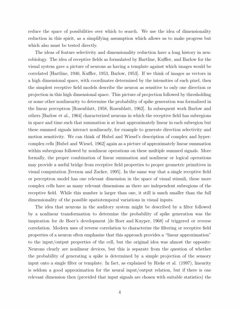
reduce the space of possibilities over which to search. We use the idea of dimensionality

reduction in this spirit, as a simplifying assumption which allows us to make progress but

which also must be tested directly.

The ideas of feature selectivity and dimensionality reduction have a long history in neu-

robiology. The idea of receptive fields as formulated by Hartline, Kuffler, and Barlow for the

visual system gave a picture of neurons as having a template against which images would be

correlated [Hartline, 1940, Kuffler, 1953, Barlow, 1953]. If we think of images as vectors in

a high dimensional space, with coordinates determined by the intensities of each pixel, then

the simplest receptive field models describe the neuron as sensitive to only one direction or

projection in this high dimensional space. This picture of projection followed by thresholding

or some other nonlinearity to determine the probability of spike generation was formalized in

the linear perceptron [Rosenblatt, 1958, Rosenblatt, 1962]. In subsequent work Barlow and

others [Barlow et al., 1964] characterized neurons in which the receptive field has subregions

in space and time such that summation is at least approximately linear in each subregion but

these summed signals interact nonlinearly, for example to generate direction selectivity and

motion sensitivity. We can think of Hubel and Wiesel’s description of complex and hyper-

complex cells [Hubel and Wiesel, 1962] again as a picture of approximately linear summation

within subregions followed by nonlinear operations on these multiple summed signals. More

formally, the proper combination of linear summation and nonlinear or logical operations

may provide a useful bridge from receptive field properties to proper geometric primitives in

visual computation [Iverson and Zucker, 1995]. In the same way that a single receptive field

or perceptron model has one relevant dimension in the space of visual stimuli, these more

complex cells have as many relevant dimensions as there are independent subregions of the

receptive field. While this number is larger than one, it still is much smaller than the full

dimensionality of the possible spatiotemporal variations in visual inputs.

The idea that neurons in the auditory system might be described by a filter followed

by a nonlinear transformation to determine the probability of spike generation was the

inspiration for de Boer’s development [de Boer and Kuyper, 1968] of triggered or reverse

correlation. Modern uses of reverse correlation to characterize the filtering or receptive field

properties of a neuron often emphasize that this approach provides a “linear approximation”

to the input/output properties of the cell, but the original idea was almost the opposite:

Neurons clearly are nonlinear devices, but this is separate from the question of whether

the probability of generating a spike is determined by a simple projection of the sensory

input onto a single filter or template. In fact, as explained by Rieke et al. (1997), linearity

is seldom a good approximation for the neural input/output relation, but if there is one

relevant dimension then (provided that input signals are chosen with suitable statistics) the

4

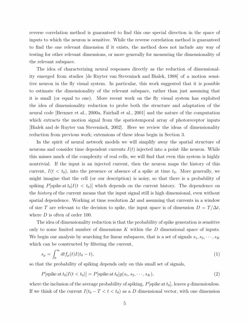
reverse correlation method is guaranteed to find this one special direction in the space of

inputs to which the neuron is sensitive. While the reverse correlation method is guaranteed

to find the one relevant dimension if it exists, the method does not include any way of

testing for other relevant dimensions, or more generally for measuring the dimensionality of

the relevant subspace.

The idea of characterizing neural responses directly as the reduction of dimensional-

ity emerged from studies [de Ruyter van Steveninck and Bialek, 1988] of a motion sensi-

tive neuron in the fly visual system. In particular, this work suggested that it is possible

to estimate the dimensionality of the relevant subspace, rather than just assuming that

it is small (or equal to one). More recent work on the fly visual system has exploited

the idea of dimensionality reduction to probe both the structure and adaptation of the

neural code [Brenner et al., 2000a, Fairhall et al., 2001] and the nature of the computation

which extracts the motion signal from the spatiotemporal array of photoreceptor inputs

[Bialek and de Ruyter van Steveninck, 2002]. Here we review the ideas of dimensionality

reduction from previous work; extensions of these ideas begin in Section 3.

In the spirit of neural network models we will simplify away the spatial structure of

neurons and consider time dependent currents I(t) injected into a point–like neuron. While

this misses much of the complexity of real cells, we will find that even this system is highly

nontrivial. If the input is an injected current, then the neuron maps the history of this

current, I(t < t0), into the presence or absence of a spike at time t0. More generally, we

might imagine that the cell (or our description) is noisy, so that there is a probability of

spiking P [spike at t0|I(t < t0)] which depends on the current history. The dependence on

the history of the current means that the input signal still is high dimensional, even without

spatial dependence. Working at time resolution ∆t and assuming that currents in a window

of size T are relevant to the decision to spike, the input space is of dimension D = T/∆t,

where D is often of order 100.

The idea of dimensionality reduction is that the probability of spike generation is sensitive

only to some limited number of dimensions K within the D dimensional space of inputs.

We begin our analysis by searching for linear subspaces, that is a set of signals s1, s2, · · · , sK

which can be constructed by filtering the current,

sµ =∫

∞

0dtfµ(t)I(t0 − t), (1)

so that the probability of spiking depends only on this small set of signals,

P [spike at t0|I(t < t0)] = P [spike at t0]g(s1, s2, · · · , sK), (2)

where the inclusion of the average probability of spiking, P [spike at t0], leaves g dimensionless.

If we think of the current I(t0 − T < t < t0) as a D dimensional vector, with one dimension

5

for each discrete sample at spacing ∆t, then the filtered signals si are linear projections of

this vector. In this formulation, characterizing the computation done by a neuron involves

three steps:

1. Estimate the number of relevant stimulus dimensions K, hopefully much less than the

original dimensionality D.

2. Identify a set of filters which project into this relevant subspace.

3. Characterize the nonlinear function g(~s).

The classical perceptron–like cell of neural network theory would have only one relevant

dimension, given by the vector of weights, and a simple form for g, typically a sigmoid.

Rather than trying to look directly at the distribution of spikes given stimuli, we follow de

Ruyter van Steveninck and Bialek (1988) and consider the distribution of signals conditional

on the response, P [I(t < t0)|spike at t0], also called the response conditional ensemble (RCE);

these are related by Bayes’ rule,

P [spike at t0|I(t < t0)]

P [spike at t0]=

P [I(t < t0)|spike at t0]

P [I(t < t0)]. (3)

We can now compute various moments of the RCE. The first moment is the spike triggered

average stimulus (STA),

STA(τ) =∫

[dI] P [I(t < t0)|spike at t0]I(t0 − τ) , (4)

which is the object that one computes in reverse correlation [de Boer and Kuyper, 1968,

Rieke et al., 1997]. If we choose the distribution of input stimuli P [I(t < t0)] to be Gaussian

white noise, then for a perceptron–like neuron sensitive to only one direction in stimulus

space, it can be shown that the STA or first moment of the response conditional ensemble

is proportional to the vector or filter f(τ) that defines this direction [Rieke et al., 1997].

Although it is a theorem that the STA is proportional to the relevant filter f(τ), in prin-

ciple it is possible that the proportionality constant is zero, most plausibly if the neuron’s

response has some symmetry, such as phase invariance in the response of high frequency

auditory neurons. It also is worth noting that what is really important in this analysis is

the Gaussian distribution of the stimuli, not the “whiteness” of the spectrum. For non-

white but Gaussian inputs the STA measures the relevant filter blurred by the correlation

function of the inputs and hence the true filter can be recovered (at least in principle) by

deconvolution. For nonGaussian signals and nonlinear neurons there is no corresponding

guarantee that the selectivity of the neuron can be separated from correlations in the stim-

ulus [Sharpee et al., 2002a].

6

To obtain more than one relevant direction (or to reveal relevant directions when sym-

metries cause the STA to vanish), we proceed to second order and compute the covariance

matrix of fluctuations around the spike triggered average,

Cspike(τ, τ′) =

∫

[dI] P [I(t < t0)|spike at t0]I(t0 − τ)I(t0 − τ ′) − STA(τ)STA(τ ′). (5)

In the same way that we compare the spike triggered average to some constant average level

of the signal in the whole experiment, we compare the covariance matrix Cspike with the

covariance of the signal averaged over the whole experiment,

Cprior(τ, τ′) =

∫

[dI] P [I(t < t0)]I(t0 − τ)I(t0 − τ ′), (6)

to construct the change in the covariance matrix

∆C = Cspike − Cprior . (7)

With time resolution ∆t in a window of duration T as above, all of these covariances are D×D

matrices. In the same way that the spike triggered average has the clearest interpretation

when we choose inputs from a Gaussian distribution, ∆C also has the clearest interpretation

in this case. Specifically, if inputs are drawn from a Gaussian distribution then it can be

shown that [Bialek and de Ruyter van Steveninck, 2002]:

1. If the neuron is sensitive to a limited set of K input dimensions as in Eq. (2), then

∆C will have only K nonzero eigenvalues.1 In this way we can measure directly the

dimensionality K of the relevant subspace.

2. If the distribution of inputs are both Gaussian and white, then the eigenvectors asso-

ciated with the nonzero eigenvalues span the same space as that spanned by the filters

{fµ(τ)}.

3. For nonwhite (correlated) but still Gaussian inputs, the eigenvectors span the space of

the filters {fµ(τ)} blurred by convolution with the correlation function of the inputs.

Thus the analysis of ∆C for neurons responding to Gaussian inputs should allow us to

identify the subspace of inputs of relevance and to test specifically the hypothesis that this

subspace is of low dimension.

Several points are worth noting. First, except in special cases, the eigenvectors of ∆C and

the filters {fµ(τ)} are not the principal components of the response conditional ensemble,

and hence this analysis of ∆C is not a principal component analysis. Second, the nonzero

1As with the STA, it is in principle possible that symmetries or accidental features of the function g(~s)would cause some of the K eigenvalues to vanish, but this is very unlikely.

7

eigenvalues of ∆C can be either positive or negative, depending on whether the variance

of inputs along that particular direction is larger or smaller in the neighborhood of a spike.

Third, although the eigenvectors span the relevant subspace, these eigenvectors do not form a

preferred coordinate system within this subspace. Finally, we emphasize that dimensionality

reduction—identification of the relevant subspace—is only the first step in our analysis of

the computation done by a neuron.

3 Measuring the success of dimensionality reduction

The claim that certain stimulus features are most relevant is in effect a model for the neu-

ron, so the next question is how to measure the effectiveness or accuracy of this model.

Several different ideas have been suggested in the literature as ways of testing models based

on linear receptive fields in the visual system [Stanley et al., 1999, Keat et al., 2001] or lin-

ear spectrotemporal receptive fields in the auditory system [Theunissen et al., 2000]. These

methods have in common that they introduce a metric to measure performance—for exam-

ple, mean square error in predicting the firing rate as averaged over some window of time.

Ideally we would like to have a performance measure which avoids any arbitrariness in the

choice of metric, and such metric free measures are provided uniquely by information theory

[Shannon, 1948, Cover and Thomas, 1991].

Observing the arrival time t0 of a single spike provides a certain amount of information

about the input signals. Since information is mutual, we can also say that knowing the

input signal trajectory I(t < t0) provides information about the arrival time of the spike. If

“details are irrelevant” then we should be able to discard these details from our description of

the stimulus and yet preserve the mutual information between the stimulus and spike arrival

times; for an abstract discussion of such selective compression see [Tishby et al., 1999]. In

constructing our low dimensional model, we represent the complete (D dimensional) stimulus

I(t < t0) by a smaller number (K < D) of dimensions ~s = (s1, s2, · · · , sK).

The mutual information I[I(t < t0); t0] is a property of the neuron itself, while the mutual

information I[~s; t0] characterizes how much our reduced description of the stimulus can tell

us about when spikes will occur. Necessarily our reduction of dimensionality causes a loss

of information, so that

I[~s; t0] ≤ I[I(t < t0); t0], (8)

but if our reduced description really captures the computation done by the neuron then

the two information measures will be very close. In particular if the neuron were described

exactly by a lower dimensional model—as for a linear perceptron, or for an integrate and

8

fire neuron [Aguera y Arcas and Fairhall, 2002]—then the two information measures would

be equal. More generally, the ratio I[~s; t0]/I[I(t < t0); t0] quantifies the efficiency of the low

dimensional model, measuring the fraction of information about spike arrival times that our

K dimensions capture from the full signal I(t < t0).

As shown by Brenner et al. (2000), the arrival time of a single spike provides an infor-

mation

I[I(t < t0); t0] ≡ Ione spike =1

T

∫ T

0dt

r(t)

rlog2

[

r(t)

r

]

, (9)

where r(t) is the time dependent spike rate, r is the average spike rate, and 〈· · ·〉 denotes

an average over time. In principle, information should be calculated as an average over the

distribution of stimuli, but the ergodicity of the stimulus justifies replacing this ensemble

average with a time average. For a deterministic system like the Hodgkin–Huxley equations,

the spike rate is a singular function of time: given the inputs I(t), spikes occur at definite

times with no randomness or irreproducibility. If we observe these responses with a time

resolution ∆t, then for ∆t sufficiently small the rate r(t) at any time t either is zero or

corresponds to a single spike occurring in one bin of size ∆t, that is r = 1/∆t. Thus the

information carried by a single spike is

Ione spike = − log2 r∆t . (10)

On the other hand, if the probability of spiking really depends only on the stimulus dimen-

sions s1, s2, · · · , sK , we can substitute

r(t)

r→ P (~s|spike at t)

P (~s). (11)

Replacing the time averages in Eq. (9) with ensemble averages, we find

I[~s; t0] ≡ I~sone spike =

∫

dKs P (~s|spike at t) log2

[

P (~s|spike at t)

P (~s)

]

; (12)

for details of these arguments see [Brenner et al., 2000b]. This allows us to compare the

information captured by the K dimensional reduced model with the true information carried

by single spikes in the spike train.

For reasons that we will discuss in the following section, and as was pointed out in

[Aguera y Arcas et al., 2001, Aguera y Arcas and Fairhall, 2002], we will be considering iso-

lated spikes, i.e. spikes separated from previous spikes by a period of silence. This has im-

portant consequences for our analysis. Most significantly, as we will be considering spikes

that occur on a background of silence, the relevant stimulus ensemble, conditioned on the

silence, is no longer Gaussian. Further, we will need to refine our information estimate.

9

The derivation of Eq. (9) makes clear that a similar formula must determine the infor-

mation carried by the occurrence time of any event, not just single spikes: we can define

an event rate in place of the spike rate, and then calculate the information carried by these

events [Brenner et al., 2000b]. In the present case we wish to compute the information ob-

tained by observing an isolated spike, or equivalently by the event silence+spike. This is

straightforward—we replace the spike rate by the rate of isolated spikes and Eq. (9) will

give us the information carried by the arrival time of a single isolated spike. The problem

is that this information includes both the information carried by the occurrence of the spike

and the information conveyed in the condition that there were no spikes in the preceding

tsilence msec [for an early discussion of the information carried by silence see de Ruyter van

Steveninck and Bialek (1988)]. We would like to separate these contributions, since our

idea of dimensionality reduction applies only the triggering of a spike, not to the temporally

extended condition of nonspiking.

To separate the information carried by the isolated spike itself, we have to ask how much

information we gain by seeing an isolated spike given that the condition for isolation has

already been met. As discussed by Brenner et al. (2000b), we can compute this information

by thinking about the distribution of times at which the isolated spike can occur. Given that

we know the input stimulus, the distribution of times at which a single isolated spike will be

observed is proportional to riso(t), the time dependent rate or peri–stimulus time histogram

for isolated spikes. With proper normalization we have

Piso(t|inputs) =1

T· 1

riso

riso(t), (13)

where T is duration of the (long) window in which we can look for the spike and riso is the

average rate of isolated spikes. This distribution has an entropy

Siso(t|inputs) = −∫ T

0dt Piso(t|inputs) log2 Piso(t|inputs) (14)

= − 1

T

∫ T

0dt

riso(t)

riso

log2

[

1

T· riso(t)

riso

]

(15)

= log2(T riso∆t) bits, (16)

where again we use the fact that for a deterministic system the time dependent rate must be

either zero or the maximum allowed by our time resolution ∆t. To compute the information

carried by a single spike we need to compare this entropy with the total entropy possible

when we don’t know the inputs.

It is tempting to think that without knowledge of the inputs, an isolated spike is equally

likely to occur anywhere in the window of size T , which leads us back to Eq. (10) with r

replaced by riso. In this case, however, we are assuming that the condition for isolation has

10

already been met. Thus, even without observing the inputs, we know that isolated spikes

can occur only in windows of time whose total length is Tsilence = T · Psilence, where Psilence is

the probability that any moment in time is at least tsilence after the most recent spike. Thus

the total entropy of isolated spike arrival times (given that the condition for silence has been

met) is reduced from log2 T to

Siso(t|silence) = log2(T · Psilence), (17)

and the information that the spike carries beyond what we know from the silence itself is

∆Iiso spike = Siso(t|silence) − Siso(t|inputs) (18)

=1

T

∫ T

0dt

riso(t)

riso

log2

[

riso(t)

riso

· Psilence

]

(19)

= − log2 (riso∆t) + log2 Psilence bits. (20)

This information, which is defined independently of any model for the feature selectivity of

the neuron, provides the benchmark against which our reduction of dimensionality will be

measured. To make the comparison, however, we need the analog of Eq. (12).

Equation (19) provides us with an expression for the information conveyed by isolated

spikes in terms of the probability that these spikes occur at particular times; this is analogous

to Eq. (9) for single (nonisolated) spikes. If we follow a path analogous to that which leads

from Eq. (9) to Eq. (12) we find an expression for the information which an isolated spike

provides about the K stimulus dimensions ~s:

∆I~siso spike =

∫

d~sP (~s|iso spike at t) log2

[

P (~s|iso spike at t)

P (~s|silence)

]

+〈log2 P (silence|~s)〉, (21)

where the prior is now also conditioned on silence: P (~s|silence), is the distribution of ~s

given that ~s is preceded by a silence of at least tsilence. Notice that this silence conditioned

distribution is not knowable a priori, and in particular it is not Gaussian; P (~s|silence) must

be sampled from data.

The last term in Eq. (21) is the entropy of a binary variable which indicates whether

particular moments in time are silent given knowledge of the stimulus. Again, since the

HH model is deterministic, this conditional entropy should be zero if we keep a complete

description of the stimulus. In fact we’re not interested in describing those features of

the stimulus which lead to silence, nor is it fair (as we will see) to judge the success of

dimensionality reduction by looking at the prediction of silence which necessarily involves

multiple dimensions. To make a meaningful comparison, then, we will assume that there is

a perfect description of the stimulus conditions leading to silence, and focus on the stimulus

11

features that trigger the isolated spike. When we approximate these features by the K

dimensional space ~s, we capture an amount of information

∆I~siso spike =

∫

d~sP (~s|iso spike at t) log2

[

P (~s|iso spike at t)

P (~s|silence)

]

. (22)

This is the information which we can compare with ∆Iiso spike in Eq. (20) to determine the

efficiency of our dimensionality reduction.

4 Characterising the Hodgkin-Huxley neuron

For completeness we begin with a brief review of the dynamics of the space–clamped Hodgkin–

Huxley neuron [Hodgkin and Huxley, 1952]. Hodgkin and Huxley modelled the dynamics of

the current through a patch of membrane with ion–specific conductances:

CdV

dt= I(t) − gKn4 (V − VK) − gNam

3h (V − VNa) − gl (V − Vl) , (23)

where I(t) is injected current, K and Na subscripts denote potassium– and sodium–related

variables, respectively, and l (for “leakage”) terms include all other ion conductances with

slower dynamics. C is the membrane capacitance. VK and VNa are ion-specific reversal

potentials, and Vl is defined such that the total voltage V is exactly zero when the membrane

is at rest. gK, gNa and gl are empirically determined maximal conductances for the different

ion species, and the gating variables n, m and h (on the interval [0, 1]) have their own voltage

dependent dynamics:

dn/dt = (0.01V + 0.1)(1 − n) exp(−0.1V ) − 0.125n exp(V/80)

dm/dt = (0.1V + 2.5)(1 − m) exp(−0.1V − 1.5) − 4m exp(V/18)

dh/dt = 0.07(1 − h) exp(0.05V ) − h exp(−0.1V − 4). (24)

We have used the original values for these parameters, except for changing the signs of the

voltages to correspond to the modern sign convention: C = 1 µF/cm2, gK = 36 mS/cm2,

gNa = 120 mS/cm2, gl = 0.3 mS/cm2, VK = −12 mV, VNa = +115 mV, Vl = +10.613 mV.

We have taken our system to be a π×302 µm2 patch of membrane. We solve these equations

numerically using fourth order Runge–Kutta integration.

The system is driven with a Gaussian random noise current I(t), generated by smoothing

a Gaussian random number stream with an exponential filter to generate a correlation time

τ . It is convenient to choose τ to be longer than the time steps of numerical integration,

since this guarantees that all functions are smooth on the scale of single time steps. Here

we will always use τ = 0.2 msec, a value that is both less than the timescale over which we

12

discretize the stimulus for analysis, and far less than the neuron’s capacitative smoothing

timescale RC ∼ 3 msec. I(t) has a standard deviation σ, but since the correlation time is

short the relevant parameter usually is the spectral density S = σ2τ ; we also add a DC offset

I0. In the following, we will consider two parameter regimes, I0 = 0, and I0 a finite value,

which leads to more periodic firing.

The integration step size is fixed at 0.05 msec. The key numerical experiments were

repeated at a step size of 0.01 msec with identical results. The time of a spike is defined as

the moment of maximum voltage, for voltages exceeding a threshold (see Fig. 1), estimated

to subsample precision by quadratic interpolation. As spikes are both very stereotyped

and very large compared to subspiking fluctuations, the precise value of this threshold is

unimportant; we have used +20 mV.

Figure 1: Spike triggered averages with standard deviations for (a) the input current I,(b) the fraction of open K+ and Na+ channels, and (c) the membrane voltage V , for theparameter regime I0 = 0 and S = 6.50 × 10−4nA2sec .

13

4.1 Qualitative description of spiking

The first step in our analysis is to use reverse correlation, Eq. (4), to determine the average

stimulus feature preceding a spike, the spike triggered average (STA). In Fig. 1(a) we display

the STA in a regime where the spectral density of the input current is 6.5 × 10−4 nA2msec.

The spike triggered averages of the gating terms n4 (proportion of open potassium channels)

and m3h (proportion of open sodium channels) and the membrane voltage V are plotted in

parts (b) and (c). The errorbars mark the standard deviation of the trajectories of these

variables.

As expected, the voltage and gating variables follow highly stereotyped trajectories during

the ∼5 msec surrounding a spike: First, the rapid opening of the sodium channels causes a

sharp membrane depolarization (or rise in V ); the slower potassium channels then open and

repolarize the membrane, leaving it at a slightly lower potential than rest. The potassium

channels close gradually, but meanwhile the membrane remains hyperpolarized and, due

to its increased permeability to potassium ions, at lower resistance. These effects make it

difficult to induce a second spike during this ∼15 msec “refractory period.” Away from spikes,

the resting levels and fluctuations of the voltage and gating variables are quite small. The

larger values evident in Fig. 1(b) and (c) by ±15 msec are due to the summed contributions

of nearby spikes.

The spike triggered average current has a largely transient form, so that spikes are on

average preceded by an upward swing in current. On the other hand, there is no obvi-

ous “bottleneck” in the current trajectories, so that the current variance is almost constant

throughout the spike. This is qualitatively consistent with the idea of dimensionality re-

duction: If the neuron ignores most of the dimensions along which the current can vary,

then the variance—which is shared almost equally among all dimensions for this near white

noise—can change only by a small amount.

4.2 Interspike interaction

Although the STA has the form of a differentiating kernel, suggesting that the neuron detects

edge–like events in the current vs. time, there must be a DC component to the cell’s response.

We recall that for constant inputs the Hodgkin–Huxley model undergoes a bifurcation to

constant frequency spiking, where the frequency is a function of the value of the input above

onset. Correspondingly the STA does not sum precisely to zero; one might think of it as

having a small integrating component that allows the system to spike under DC stimulation,

albeit only above a threshold.

The system’s tendency to periodic spiking under DC current input also is felt under

14

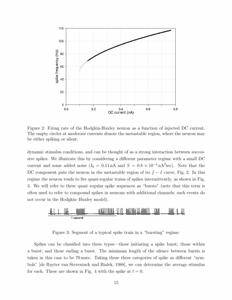
Figure 2: Firing rate of the Hodgkin-Huxley neuron as a function of injected DC current.The empty circles at moderate currents denote the metastable region, where the neuron maybe either spiking or silent.

dynamic stimulus conditions, and can be thought of as a strong interaction between succes-

sive spikes. We illustrate this by considering a different parameter regime with a small DC

current and some added noise (I0 = 0.11 nA and S = 0.8 × 10−4 nA2sec). Note that the

DC component puts the neuron in the metastable region of its f − I curve, Fig. 2. In this

regime the neuron tends to fire quasi-regular trains of spikes intermittently, as shown in Fig.

3. We will refer to these quasi–regular spike sequences as “bursts” (note that this term is

often used to refer to compound spikes in neurons with additional channels; such events do

not occur in the Hodgkin–Huxley model).

Figure 3: Segment of a typical spike train in a “bursting” regime.

Spikes can be classified into three types—those initiating a spike burst; those within

a burst; and those ending a burst. The minimum length of the silence between bursts is

taken in this case to be 70 msec. Taking these three categories of spike as different “sym-

bols” [de Ruyter van Steveninck and Bialek, 1988], we can determine the average stimulus

for each. These are shown in Fig. 4 with the spike at t = 0.

15

In this regime, the initial spike of a burst is preceded by a rapid oscillation in the current.

Spikes within a burst are affected much less by the current; the feature immediately preceding

such spikes is similar in shape to a single “wavelength” of the leading spike feature, but

is of much smaller amplitude, and is temporally compressed into the interspike interval.

Hence, although it is clear that the timing of a spike within a burst is determined largely

by the timing of the previous spike, the current plays some role in affecting the precise

placement. This also demonstrates that the shape of the STA is not the same for all spikes;

it depends strongly and nontrivially on the time to the previous spike, and this is related

to the observation that subtly different patterns of two or three spikes correspond to very

different average stimuli [de Ruyter van Steveninck and Bialek, 1988]. For a reader of the

spike code, a spike within a burst conveys a different message about the input than the spike

at the onset of the burst. Finally, the feature ending a burst has a very similar form to the

onset feature, but reversed in time. Thus, to a good approximation, the absence of a spike

at the end of a burst can be read as the opposite of the onset of the burst.

Figure 4: Spike triggered averages, derived from spikes leading (“on”), inside (“burst”)and ending (“off”) a burst. The parameters of this bursting regime are I0 = 0.11 nA andS = 0.8×10−4 nA2sec. Note that the burst-ending spike average is, by construction, identicalto that of any other within-burst spike for t < 0.

In summary, this regime of the HH neuron is similar to a “flip-flop”, or 1-bit memory.

Like its electronic analogue, the neuron’s memory is preserved by a feedback loop, here

implemented by the interspike interaction. Large fluctuations in the input current at a

certain frequency “flip” or “flop” the neuron between its silent and spiking states. However,

while the neuron is spiking, further details of the input signal are transmitted by precise

spike timing within a burst. If we calculate the spike triggered average of all spikes for this

regime, without regard to their position within a burst, then as shown in Fig. 5 the relatively

well localized leading spike oscillation of Fig. 4 is replaced by a long-lived oscillating function

resulting from the spike periodicity. This is shown explicitly by comparing the overall STA

with the spike autocorrelation, also shown in Fig. 5. This same effect is seen in the STA

16

of the burst spikes, which in fact dominates the overall average. Prediction of spike timing

using such an STA would be computationally difficult, due to its extension in time, but,

more seriously, unsuccessful, as most of the function is an artifact of the spike history rather

than the effect of the stimulus.

Figure 5: Overall spike triggered average in the bursty regime, showing the ringing due tothe tendency to periodic firing; plotted in grey is the spike autocorrelation, showing the sameoscillations.

While the effects of spike interaction are interesting, and should be included in a complete

model for spike generation, we wish here to consider only the current’s role in initiating spikes.

Therefore, as we have argued elsewhere, we limit ourselves initially to the cases in which inter-

spike interaction plays no role [Aguera y Arcas et al., 2001, Aguera y Arcas and Fairhall, 2002].

These “isolated” spikes can be defined as spikes preceded by a silent period tsilence long enough

to ensure decoupling from the timing of the previous spike. A reasonable choice for tsilence

can be inferred directly from the interspike interval distribution P (∆t), illustrated in Fig. 6.

For the HH model, as in simpler models and many real neurons [Brenner et al., 1998], the

form of P (∆t) has three noteworthy features: a refractory “hole” during which another spike

is unlikely to occur, a strong mode at the preferred firing frequency, and an exponentially

decaying, or Poisson tail. The details of all three of these features are functions of the pa-

rameters of the stimulus, and certain regimes may be dominated by only one or two features.

The emergence of Poisson statistics in the tail of the distribution implies that these events

are independent, so we can infer that the system has lost memory of the previous spike. We

17

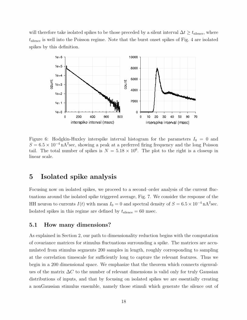
will therefore take isolated spikes to be those preceded by a silent interval ∆t ≥ tsilence, where

tsilence is well into the Poisson regime. Note that the burst onset spikes of Fig. 4 are isolated

spikes by this definition.

Figure 6: Hodgkin-Huxley interspike interval histogram for the parameters I0 = 0 andS = 6.5 × 10−4 nA2sec, showing a peak at a preferred firing frequency and the long Poissontail. The total number of spikes is N = 5.18 × 106. The plot to the right is a closeup inlinear scale.

5 Isolated spike analysis

Focusing now on isolated spikes, we proceed to a second–order analysis of the current fluc-

tuations around the isolated spike triggered average, Fig. 7. We consider the response of the

HH neuron to currents I(t) with mean I0 = 0 and spectral density of S = 6.5× 10−4 nA2sec.

Isolated spikes in this regime are defined by tsilence = 60 msec.

5.1 How many dimensions?

As explained in Section 2, our path to dimensionality reduction begins with the computation

of covariance matrices for stimulus fluctuations surrounding a spike. The matrices are accu-

mulated from stimulus segments 200 samples in length, roughly corresponding to sampling

at the correlation timescale for sufficiently long to capture the relevant features. Thus we

begin in a 200 dimensional space. We emphasize that the theorem which connects eigenval-

ues of the matrix ∆C to the number of relevant dimensions is valid only for truly Gaussian

distributions of inputs, and that by focusing on isolated spikes we are essentially creating

a nonGaussian stimulus ensemble, namely those stimuli which generate the silence out of

18

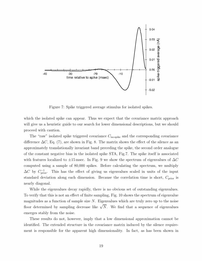
Figure 7: Spike triggered average stimulus for isolated spikes.

which the isolated spike can appear. Thus we expect that the covariance matrix approach

will give us a heuristic guide to our search for lower dimensional descriptions, but we should

proceed with caution.

The “raw” isolated spike triggered covariance Ciso spike and the corresponding covariance

difference ∆C, Eq. (7), are shown in Fig. 8. The matrix shows the effect of the silence as an

approximately translationally invariant band preceding the spike, the second order analogue

of the constant negative bias in the isolated spike STA, Fig.7. The spike itself is associated

with features localized to ±15 msec. In Fig. 9 we show the spectrum of eigenvalues of ∆C

computed using a sample of 80,000 spikes. Before calculating the spectrum, we multiply

∆C by C−1prior. This has the effect of giving us eigenvalues scaled in units of the input

standard deviation along each dimension. Because the correlation time is short, Cprior is

nearly diagonal.

While the eigenvalues decay rapidly, there is no obvious set of outstanding eigenvalues.

To verify that this is not an effect of finite sampling, Fig. 10 shows the spectrum of eigenvalue

magnitudes as a function of sample size N . Eigenvalues which are truly zero up to the noise

floor determined by sampling decrease like√

N . We find that a sequence of eigenvalues

emerges stably from the noise.

These results do not, however, imply that a low dimensional approximation cannot be

identified. The extended structure in the covariance matrix induced by the silence require-

ment is responsible for the apparent high dimensionality. In fact, as has been shown in

19

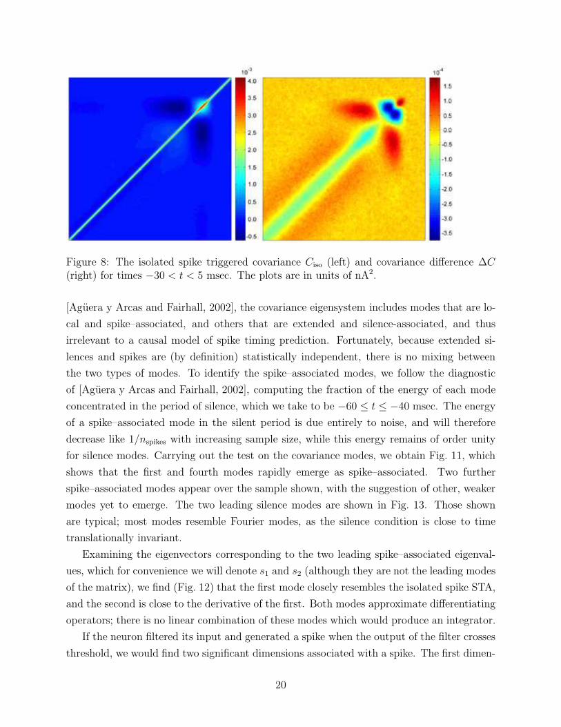
Figure 8: The isolated spike triggered covariance Ciso (left) and covariance difference ∆C(right) for times −30 < t < 5 msec. The plots are in units of nA2.

[Aguera y Arcas and Fairhall, 2002], the covariance eigensystem includes modes that are lo-

cal and spike–associated, and others that are extended and silence-associated, and thus

irrelevant to a causal model of spike timing prediction. Fortunately, because extended si-

lences and spikes are (by definition) statistically independent, there is no mixing between

the two types of modes. To identify the spike–associated modes, we follow the diagnostic

of [Aguera y Arcas and Fairhall, 2002], computing the fraction of the energy of each mode

concentrated in the period of silence, which we take to be −60 ≤ t ≤ −40 msec. The energy

of a spike–associated mode in the silent period is due entirely to noise, and will therefore

decrease like 1/nspikes with increasing sample size, while this energy remains of order unity

for silence modes. Carrying out the test on the covariance modes, we obtain Fig. 11, which

shows that the first and fourth modes rapidly emerge as spike–associated. Two further

spike–associated modes appear over the sample shown, with the suggestion of other, weaker

modes yet to emerge. The two leading silence modes are shown in Fig. 13. Those shown

are typical; most modes resemble Fourier modes, as the silence condition is close to time

translationally invariant.

Examining the eigenvectors corresponding to the two leading spike–associated eigenval-

ues, which for convenience we will denote s1 and s2 (although they are not the leading modes

of the matrix), we find (Fig. 12) that the first mode closely resembles the isolated spike STA,

and the second is close to the derivative of the first. Both modes approximate differentiating

operators; there is no linear combination of these modes which would produce an integrator.

If the neuron filtered its input and generated a spike when the output of the filter crosses

threshold, we would find two significant dimensions associated with a spike. The first dimen-

20

Figure 9: The leading 64 eigenvalues of the isolated spike triggered covariance, after accu-mulating 80,000 spikes.

sion would correspond simply to the filter, as the variance in this dimension is reduced to zero

(for a noiseless system) at the occurrence of a spike. As the threshold is always crossed from

below, the stimulus projection onto the filter’s derivative must be positive, again resulting

in a reduced variance. It is tempting to suggest, then, that filtered threshold crossing is a

good approximation to the HH model, but we will see that this is not correct.

5.2 Evaluating the nonlinearity

At each instant of time we can find the projections of the stimulus along the leading spike–

associated dimensions s1 and s2. By construction, the distribution of these signals over the

whole experiment, P (s1, s2), is Gaussian. The appropriate prior for the isolation condition,

P (s1, s2|silence), differs only subtly from the Gaussian prior. On the other hand, for each

spike we obtain a sample from the distribution P (s1, s2|iso spike at t0), leading to the picture

in Fig. 14. The prior and spike conditional distributions are clearly better separated in two

dimensions than in one, which means that the two dimensional description captures more

information than projection onto the spike triggered average alone. Surprisingly, the spike

conditional distribution is curved, unlike what we would expect for a simple thresholding

device. Furthermore, the eigenvalue of ∆C which we associate with the direction of thresh-

21

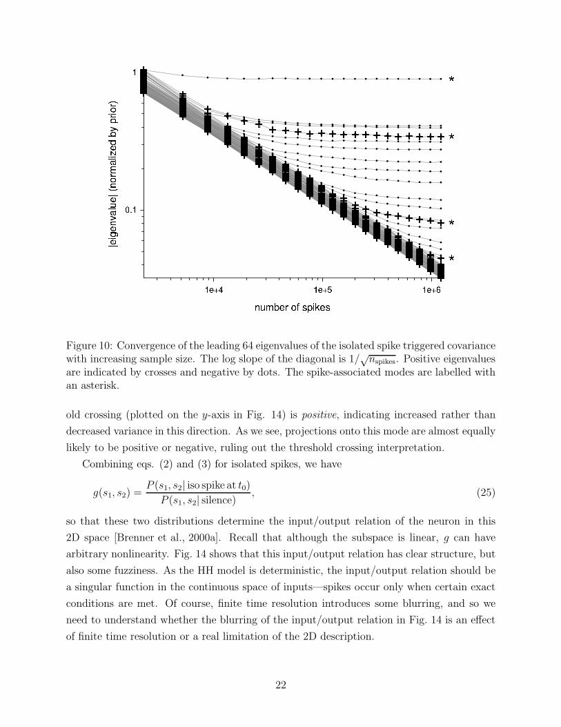
Figure 10: Convergence of the leading 64 eigenvalues of the isolated spike triggered covariancewith increasing sample size. The log slope of the diagonal is 1/

√nspikes. Positive eigenvalues

are indicated by crosses and negative by dots. The spike-associated modes are labelled withan asterisk.

old crossing (plotted on the y-axis in Fig. 14) is positive, indicating increased rather than

decreased variance in this direction. As we see, projections onto this mode are almost equally

likely to be positive or negative, ruling out the threshold crossing interpretation.

Combining eqs. (2) and (3) for isolated spikes, we have

g(s1, s2) =P (s1, s2| iso spike at t0)

P (s1, s2| silence), (25)

so that these two distributions determine the input/output relation of the neuron in this

2D space [Brenner et al., 2000a]. Recall that although the subspace is linear, g can have

arbitrary nonlinearity. Fig. 14 shows that this input/output relation has clear structure, but

also some fuzziness. As the HH model is deterministic, the input/output relation should be

a singular function in the continuous space of inputs—spikes occur only when certain exact

conditions are met. Of course, finite time resolution introduces some blurring, and so we

need to understand whether the blurring of the input/output relation in Fig. 14 is an effect

of finite time resolution or a real limitation of the 2D description.

22

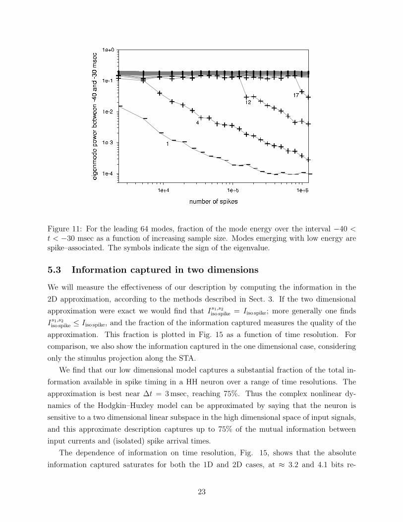
Figure 11: For the leading 64 modes, fraction of the mode energy over the interval −40 <t < −30 msec as a function of increasing sample size. Modes emerging with low energy arespike–associated. The symbols indicate the sign of the eigenvalue.

5.3 Information captured in two dimensions

We will measure the effectiveness of our description by computing the information in the

2D approximation, according to the methods described in Sect. 3. If the two dimensional

approximation were exact we would find that Is1,s2

iso spike = Iiso spike; more generally one finds

Is1,s2

iso spike ≤ Iiso spike, and the fraction of the information captured measures the quality of the

approximation. This fraction is plotted in Fig. 15 as a function of time resolution. For

comparison, we also show the information captured in the one dimensional case, considering

only the stimulus projection along the STA.

We find that our low dimensional model captures a substantial fraction of the total in-

formation available in spike timing in a HH neuron over a range of time resolutions. The

approximation is best near ∆t = 3 msec, reaching 75%. Thus the complex nonlinear dy-

namics of the Hodgkin–Huxley model can be approximated by saying that the neuron is

sensitive to a two dimensional linear subspace in the high dimensional space of input signals,

and this approximate description captures up to 75% of the mutual information between

input currents and (isolated) spike arrival times.

The dependence of information on time resolution, Fig. 15, shows that the absolute

information captured saturates for both the 1D and 2D cases, at ≈ 3.2 and 4.1 bits re-

23

Figure 12: Modes 1 and 4 of the spike triggered covariance, which are the leading spike–associated modes.

spectively. Hence, for smaller ∆t, the information fraction captured drops. The model

provides, at its best, a time resolution of 3 msec, so that information carried by more pre-

cise spike timing is lost in our low dimensional projection. Might this missing information

be important for a real neuron? Stochastic HH simulations with realistic channel densi-

ties suggest that the timing of spikes in response to white noise stimuli is reproducible to

within 1–2 msec [Schneidman et al., 1998], a figure which is comparable to what is observed

for pyramidal cells in vitro [Mainen and Sejnowski, 1995], as well in vivo in the fly’s vi-

sual system [de Ruyter van Steveninck et al., 1997, Lewen et al., 2001], the vertebrate retina

[Berry II et al., 1997], the cat LGN [Reinagel and Reid, 2000] and the bat auditory cortex

[Dear et al., 1993]. This suggests that such timing details may indeed be important. We

must therefore ask why our approximation seems to carry an inherent time resolution lim-

itation, and why, even at its optimal resolution, the full information in the spike is not

recovered.

For many purposes, recovering 75% of the information at ∼ 3 msec resolution might be

considered a resounding success. On the other hand, with such a simple underlying model

we would hope for a more compelling conclusion. From a methodological point of view it

behooves us to ask what we are missing in our 2D model, and perhaps the methods we use

in finding the missing information in the present case will prove applicable more generally.

24

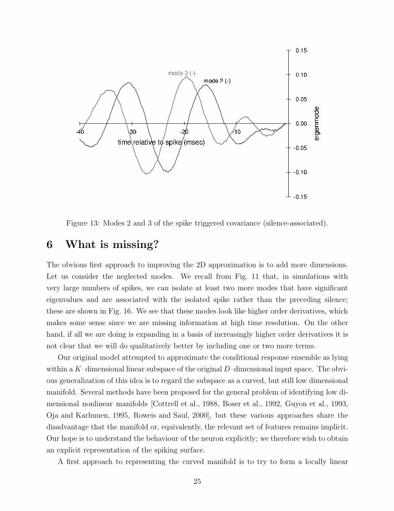
Figure 13: Modes 2 and 3 of the spike triggered covariance (silence-associated).

6 What is missing?

The obvious first approach to improving the 2D approximation is to add more dimensions.

Let us consider the neglected modes. We recall from Fig. 11 that, in simulations with

very large numbers of spikes, we can isolate at least two more modes that have significant

eigenvalues and are associated with the isolated spike rather than the preceding silence;

these are shown in Fig. 16. We see that these modes look like higher order derivatives, which

makes some sense since we are missing information at high time resolution. On the other

hand, if all we are doing is expanding in a basis of increasingly higher order derivatives it is

not clear that we will do qualitatively better by including one or two more terms.

Our original model attempted to approximate the conditional response ensemble as lying

within a K–dimensional linear subspace of the original D–dimensional input space. The obvi-

ous generalization of this idea is to regard the subspace as a curved, but still low dimensional

manifold. Several methods have been proposed for the general problem of identifying low di-

mensional nonlinear manifolds [Cottrell et al., 1988, Boser et al., 1992, Guyon et al., 1993,

Oja and Karhunen, 1995, Roweis and Saul, 2000], but these various approaches share the

disadvantage that the manifold or, equivalently, the relevant set of features remains implicit.

Our hope is to understand the behaviour of the neuron explicitly; we therefore wish to obtain

an explicit representation of the spiking surface.

A first approach to representing the curved manifold is to try to form a locally linear

25

Figure 14: 104 spike conditional stimuli (or “spike histories”) projected along the first twocovariance modes. The axes are in units of standard deviation on the prior Gaussian distri-bution. The circles, from the inside out, enclose all but 10−1, 10−2, . . . , 10−8 of the prior.

tiling. Beginning with first order statistics, there is only one natural direction along which

to parametrize—the spike triggered average. We sort the stimulus histories according to

their projection onto the spike triggered average, divide them into bins, and recompute

the averages over the bins individually. If these conditional averages have a component

orthogonal to the overall STA, then this component is a locally meaningful basis vector for

the manifold at that “slice.”. This procedure results in the family of curves orthogonal to

the STA shown in Fig. 17.

The analysis shown here was carried out with 80,000 isolated spikes; note that a similar

number of spikes cannot resolve more than two spike–associated covariance modes in the

covariance matrix analysis. The spikes were divided into eight bins according to their pro-

jection onto the STA, with 10,000 spikes per bin. Applying singular value decomposition to

the family of curves shows that there are at least four significant independent directions in

26

Figure 15: Bits per spike (left) and fraction of the theoretical limit (right) of timing infor-mation in a single spike at a given temporal resolution captured by projection onto the STAalone (triangles), and projection onto ∆C covariance modes 1 and 2 (circles).

stimulus space apart from the STA. This gives us a lower bound on the embedding dimension

of the manifold.

Computing the information as a function of ∆t using this locally linear model, we obtain

the curve shown in Fig.18, where the results can be compared against the information found

from the STA alone and from the covariance modes. The information from the new model

captures a maximum of 4.8 bits, recovering ∼ 90% of the information at a time resolution

of approximately 1 msec.

7 Discussion

The Hodgkin–Huxley equations describe the dynamics of four degrees of freedom, and almost

since these equations first were written down there have been attempts to find simplifications

or reductions. FitzHugh and Nagumo proposed a two dimensional system of equations

that approximate the HH model [Fitzhugh, 1961, Nagumo et al., 1962], and this has the

advantage that one can visualize the trajectories directly in the plane and thus achieve an

intuitive graphical understanding of the dynamics and its dependence on parameters. The

need for reduction in the sense pioneered by FitzHugh and by Nagumo et al. has become

only more urgent with the growing use of increasingly complex HH–style model neurons with

many different channel types. With this problem in mind, Kepler, Abbott and Marder have

introduced reduction methods which are more systematic, making use of the difference in

timescales among the gating variables [Kepler et al., 1992, Abbott and Kepler, 1990].

In the presence of constant current inputs, it makes sense to describe the Hodgkin–Huxley

equations as a four dimensional autonomous dynamical system; by well known methods in

27

Figure 16: The two next spike–associated modes. These resemble higher-order derivatives.

dynamical systems theory, one could consider periodic input currents by adding an extra

dimension. The question asked by FitzHugh and Nagumo was whether this four or five

dimensional description could be reduced to two or three dimensions.

Closer in spirit to our approach is the work by Kistler et al., who focused in particular on

the interaction among successive action potentials [Kistler et al., 1997]. They argued that

one could approximate the Hodgkin–Huxley model by a nearly linear dynamical system with

a threshold, identifying threshold crossing with spiking, provided that each spike generated

either a change in threshold or an effective input current which influences the generation of

subsequent spikes.

The notion of model dimensionality considered here is distinct from the dynamical sys-

tems perspective in which one simply counts the system’s degrees of freedom. Here we are

attempting to find a description of the dynamics which is essentially functional or compu-

tational. We have identified the output of the system as spike times, and our aim is to

construct as complete a description as possible of the mapping between input and output.

The dimensionality of our model is that of the space of inputs relevant for this mapping.

There is no necessary relationship between these two notions of dimensionality. For example,

in a neural network with two attractors, a system described by a potentially large number

of variables, there might be a simple rule (perhaps even a linear filter) which allows us to

look at the inputs to the network and determine the times at which the switching events will

occur. Conversely, once we leave the simplified world of constant or periodic inputs, even

28

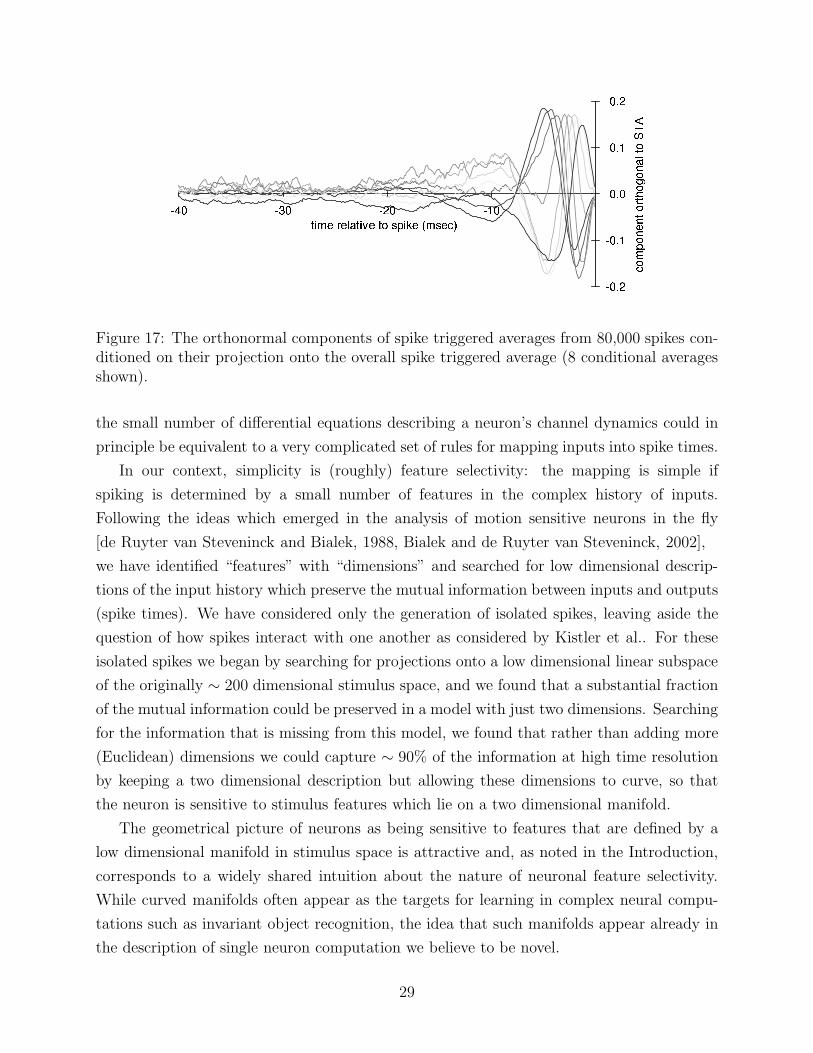
Figure 17: The orthonormal components of spike triggered averages from 80,000 spikes con-ditioned on their projection onto the overall spike triggered average (8 conditional averagesshown).

the small number of differential equations describing a neuron’s channel dynamics could in

principle be equivalent to a very complicated set of rules for mapping inputs into spike times.

In our context, simplicity is (roughly) feature selectivity: the mapping is simple if

spiking is determined by a small number of features in the complex history of inputs.

Following the ideas which emerged in the analysis of motion sensitive neurons in the fly

[de Ruyter van Steveninck and Bialek, 1988, Bialek and de Ruyter van Steveninck, 2002],

we have identified “features” with “dimensions” and searched for low dimensional descrip-

tions of the input history which preserve the mutual information between inputs and outputs

(spike times). We have considered only the generation of isolated spikes, leaving aside the

question of how spikes interact with one another as considered by Kistler et al.. For these

isolated spikes we began by searching for projections onto a low dimensional linear subspace

of the originally ∼ 200 dimensional stimulus space, and we found that a substantial fraction

of the mutual information could be preserved in a model with just two dimensions. Searching

for the information that is missing from this model, we found that rather than adding more

(Euclidean) dimensions we could capture ∼ 90% of the information at high time resolution

by keeping a two dimensional description but allowing these dimensions to curve, so that

the neuron is sensitive to stimulus features which lie on a two dimensional manifold.

The geometrical picture of neurons as being sensitive to features that are defined by a

low dimensional manifold in stimulus space is attractive and, as noted in the Introduction,

corresponds to a widely shared intuition about the nature of neuronal feature selectivity.

While curved manifolds often appear as the targets for learning in complex neural compu-

tations such as invariant object recognition, the idea that such manifolds appear already in

the description of single neuron computation we believe to be novel.

29

Figure 18: Bits per spike (left) and fraction of the theoretical limit (right) of timing in-formation in a single spike at a given temporal resolution captured by the locally lineartiling ‘twist’ model (diamonds), compared to models using the STA alone (triangles), andprojection onto ∆C covariance modes 1 and 2 (circles).

While we have exploited the fact that long simulations of the Hodgkin–Huxley model

are quite tractable to generate large amounts of “data” for our analysis, it is important

that, in the end, our construction of a curved manifold as the relevant stimulus subspace in-

volves a series of computations which are just simple generalizations of the conventional

reverse correlation or spike triggered average. This suggests that our approach can be

applied to real neurons without requiring qualitatively larger data sets than might have

been needed for a careful reverse correlation analysis. In the same spirit, recent work has

shown how covariance matrix analysis of the fly’s motion sensitive neurons can reveal non-

linear computations in a four dimensional subspace using data sets of fewer than 104 spikes

[Bialek and de Ruyter van Steveninck, 2002]. Low dimensional (linear) subspaces can be

found even in the response of model neurons to naturalistic inputs if one searches directly

for dimensions which capture the largest fraction of the mutual information between inputs

and spikes [Sharpee et al., 2002a], and again the errors involved in identifying the relevant

dimensions are comparable to the errors in reverse correlation [Sharpee et al., 2002b]. All of

these results point to the practical feasibility of describing real neurons in terms of nonlinear

computation on low dimensional relevant subspaces in a high dimensional stimulus space.

Our reduced model of the Hodgkin–Huxley neuron both illustrates a novel approach to

dimensional reduction and gives new insight into the computation performed by the neuron.

The reduced model is essentially that of an edge detector for current trajectories, but is

sensitive to a further stimulus parameter, producing a curved manifold. An interpretation

of this curvature will be presented in a forthcoming manuscript. This curved representation

is able to capture almost all information that isolated spikes convey about the stimulus, or

30

conversely, allow us to predict isolated spike times with high temporal precision from the

stimulus. The emergence of a low dimensional curved manifold in a model as simple as

the Hodgkin–Huxley neuron suggests that such a description may be also appropriate for

biological neurons.

Our approach is limited in that we address only isolated spikes. This restricted class

of spikes nonetheless has biological relevance; for example, in vertebrate retinal ganglion

cells [Berry II and Meister, 1999] and in rat somatosensory cortex [Panzeri et al., 2001], the

first spike of a burst has been shown to convey distinct (and the majority of the) infor-

mation. However, a clear next step in this program is to extend our formalism to take

into account interspike interaction. For neurons or models with explicit long timescales,

adaptation induces very long range history dependence which complicates the issue of spike

interactions considerably. A full understanding of the interaction between stimulus and

spike history will therefore, in general, involve understanding the meanings of spike patterns

[de Ruyter van Steveninck and Bialek, 1988, Brenner et al., 2000b] and the influence of the

larger statistical context [Fairhall et al., 2001]. Our results point to the need for a more

parsimonious description of self–excitation, even for the simple case of dependence only on

the last spike time.

We would like to close by reminding the reader of the more ambitious goal of building

bridges between the burgeoning molecular level description of neurons and the functional or

computational level. Armed with a description of spike generation as a nonlinear operation

on a low dimensional, curved manifold in the space of inputs, it is natural to ask how the

details of this computational picture are related to molecular mechanisms. Are neurons

with more different types of ion channels sensitive to more stimulus dimensions, or do they

implement more complex nonlinearities in a low dimensional space? Are adaptation and

modulation mechanisms that change the nonlinearity separable from those which change the

dimensions to which the cell is sensitive? Finally, while we have shown how a low dimensional

description can be constructed numerically from observations of the input/output properties

of the neuron, one would like to understand analytically why such a description emerges and

whether it emerges universally from the combinations of channel dynamics selected by real

neurons.

Acknowledgments

We thank N. Brenner for discussions at the start of this work, and M. Berry for comments

on the manuscript.

31

References

[Abbott and Kepler, 1990] Abbott, L. F. and Kepler, T. (1990). Model neurons: from

hodgkin-huxley to hopfield. In Statistical Mechanics of Neural Networks, pages 5–18,

Berlin. Springer–Verlag.

[Aguera y Arcas, 1998] Aguera y Arcas, B. (1998). Reducing the neuron: a computational

approach. Master’s thesis, Princeton University.

[Aguera y Arcas et al., 2001] Aguera y Arcas, B., Bialek, W., and Fairhall, A. L. (2001).

What can a single neuron compute? In Leen, T., Dietterich, T., and Tresp, V., editors,

Advances in Neural Information Processing Systems 13, pages 75–81. MIT Press.

[Aguera y Arcas and Fairhall, 2002] Aguera y Arcas, B. and Fairhall, A. (2002). What

causes a neuron to spike? submitted.

[Barlow, 1953] Barlow, H. B. (1953). Summation and inhibition in the frog’s retina. J.

Physiol., 119:69–88.

[Barlow et al., 1964] Barlow, H. B., Hill, R. M., and Levick, W. R. (1964). Retinal ganglion

cells responding selectively to direction and speed of image motion in the rabbit. J.

Physiol., 173:377–407.

[Berry II and Meister, 1999] Berry II, M. J. and Meister, M. (1999). The neural code of the

retina. Neuron, 22:435–450.

[Berry II et al., 1997] Berry II, M. J., Warland, D., and Meister, M. (1997). The structure

and precision of retinal spike trains. Proc. Natl. Acad. Sci. U.S.A., 94:5411–5416.

[Bialek and de Ruyter van Steveninck, 2002] Bialek, W. and de Ruyter van Steveninck,

R. R. (2002). Features and dimensions: motion estimation in fly vision. in preparation.

[Boser et al., 1992] Boser, B. E., Guyon, I. M., and Vapnik, V. N. (1992). A training algo-

rithm for optimal margin classifers. In Haussler, D., editor, 5th Annual ACM Workshop

on COLT, pages 144–152, Pittsburgh, PA. ACM Press.

[Bray, 1995] Bray, D. (1995). Protein molecules as computational elements in living cells.

Nature, 376:307–312.

[Brenner et al., 1998] Brenner, N., Agam, O., Bialek, W., and de Ruyter van

Steveninck, R. R. (1998). Universal statistical behavior of neural spike trains.

Phys. Rev. Lett., 81:4000–4003. See also Statistical properties of spike trains:

32

universal and stimulus–dependent aspects, Phys. Rev. E 66, 031907 (2002);

http://xxx.lanl.gov/abs/physics/9801026 and http://xxx.lanl.gov/abs/physics/9902061.

[Brenner et al., 2000a] Brenner, N., Bialek, W., and de Ruyter van Steveninck, R. R.

(2000a). Adaptive rescaling maximizes information transmission. Neuron, 26:695–702.

[Brenner et al., 2000b] Brenner, N., Strong, S., Koberle, R., Bialek, W., and de Ruyter van

Steveninck, R. R. (2000b). Synergy in a neural code. Neural Comp., 12:1531–1552. See

also http://xxx.lanl.gov/abs/physics/9902067.

[Cottrell et al., 1988] Cottrell, G. W., Munro, P., and Zipser, D. (1988). Image compression

by back propagation: a demonstration of extensional programming. In Sharkey, N., editor,

Models of cognition: a review of cognitive science, volume 2, pages 208–240, Norwood, NJ.

Abbex.

[Cover and Thomas, 1991] Cover, T. M. and Thomas, J. A. (1991). Elements of Information

Theory. John Wiley & Sons, Inc., New York.

[de Boer and Kuyper, 1968] de Boer, E. and Kuyper, P. (1968). Triggered correlation. IEEE

Trans. Biomed. Eng., 15:169–179.

[de Ruyter van Steveninck and Bialek, 1988] de Ruyter van Steveninck, R. R. and Bialek,

W. (1988). Real-time performance of a movement sensitive in the blowfly visual system:

information transfer in short spike sequences. Proc. Roy. Soc. Lond. B, 234:379–414.

[de Ruyter van Steveninck et al., 1997] de Ruyter van Steveninck, R., Lewen, G. D., Strong,

S. P., Koberle, R., and Bialek, W. (1997). Reproducibility and variability in neural spike

trains. Science, 275:1805–1808.

[Dear et al., 1993] Dear, S. P., Simmons, J. A., and Fritz, J. (1993). A possible neuronal

basis for representation of acoustic scenes in auditory cortex of the big brown bat. Nature,

364:620–623.

[Fairhall et al., 2001] Fairhall, A., Lewen, G., Bialek, W., and de Ruyter van Steveninck,

R. R. (2001). Efficiency and ambiguity in an adaptive neural code. Nature, 412:787–792.

[Fitzhugh, 1961] Fitzhugh, R. (1961). Impulse and physiological states in models of nerve

membrane. Biophysics J., 1:445–466.

[Guyon et al., 1993] Guyon, I. M., Boser, B. E., and Vapnik, V. N. (1993). Automatic

capacity tuning of very large vc-dimension classifiers. In Hanson, S. J., Cowan, J. D., and

33

Giles, C., editors, Advances in Neural Information Processing Systems 5, pages 147–155,

San Mateo, CA. Morgan Kaufmann.

[Hartline, 1940] Hartline, H. K. (1940). The receptive fields of optic nerve fibres. Amer. J.

Physiol., 130:690–699.

[Hille, 1992] Hille, B. (1992). Ionic channels of excitable membranes. Sinaur, Sunderland,

Massachusetts.

[Hodgkin and Huxley, 1952] Hodgkin, A. L. and Huxley, A. F. (1952). A quantitative de-

scription of membrane current and its application to conduction and excitation in nerve.

J. Physiol., 463:391–407.

[Hubel and Wiesel, 1962] Hubel, D. H. and Wiesel, T. N. (1962). Receptive fields, binocular

interaction and functional architecture in the cat’s visual cortex. J. Physiol. (Lond.),

160:106–154.

[Iverson and Zucker, 1995] Iverson, L. and Zucker, S. W. (1995). Logical/linear operators

for image curves. IEEE Trans. Pattern Analysis and Machine Intelligence, 17:982–996.

[Keat et al., 2001] Keat, J., Reinagel, P., Reid, R. C., and Meister, M. (2001). Predicting

every spike: a model for the responses of visual neurons. Neuron, 30(3):803–817.

[Kepler et al., 1992] Kepler, T., Abbott, L. F., and Marder, E. (1992). Reduction of

conductance-based neuron models. Biological Cybernetics, 66:381–387.

[Kistler et al., 1997] Kistler, W., Gerstner, W., and van Hemmen, J. L. (1997). Reduction of

the Hodgkin-Huxley equations to a single-variable threshold model. Neural Computation,

9:1015–1045.

[Koch, 1999] Koch, C. (1999). Biophysics of computation: information processing in single

neurons. Oxford University Press, New York.

[Kuffler, 1953] Kuffler, S. W. (1953). Discharge patterns and functional organization of

mammalian retina. J. Neurophysiol., 16:37–68.

[Lewen et al., 2001] Lewen, G. D., Bialek, W., and de Ruyter van Steveninck, R. R. (2001).

Neural coding of naturalistic motion stimuli. Network, 12:317–329.

[Mainen and Sejnowski, 1995] Mainen, Z. F. and Sejnowski, T. J. (1995). Reliability of spike

timing in neocortical neurons. Science, 268:1503–1506.

34

[Nagumo et al., 1962] Nagumo, J., Arimoto, S., and Yoshikawa, Z. (1962). An active pulse

transmission line simulating nerve axon. Proc. IRE, 50:2061–2071.

[Oja and Karhunen, 1995] Oja, E. and Karhunen, J. (1995). Signal separation by nonlinear

hebbian learning. In Palaniswami, M., Attikiouzel, Y., II, R. M., Fogel, D., and Fukuda,

T., editors, Computational intelligence– a dynamic system perspective, pages 83–97, New

York. IEEE Press.

[Panzeri et al., 2001] Panzeri, S., Petersen, R., Schultz, S., Lebedev, M., and Diamond, M.

(2001). The role of spike timing in the coding of stimulus location in rat somatosensory

cortex. Neuron, 29:769–77.

[Reinagel and Reid, 2000] Reinagel, P. and Reid, R. C. (2000). Temporal coding of visual

information in the thalamus. J. Neuroscience, 20(14):5392–5400.

[Rieke et al., 1997] Rieke, F., Warland, D., Bialek, W., and de Ruyter van Steveninck, R. R.

(1997). Spikes: exploring the neural code. The MIT Press, New York.

[Rosenblatt, 1958] Rosenblatt, F. (1958). The perceptron: A probabilistic model for infor-

mation storage and organization in the brain. Psychological Review, 65:386–408.

[Rosenblatt, 1962] Rosenblatt, F. (1962). Principles of Neurodynamics. Spartan Books, New

York.

[Roweis and Saul, 2000] Roweis, S. and Saul, L. (2000). Nonlinear dimensionality reduction

by locally linear embedding. Science, 290:2323–2326.

[Schneidman et al., 1998] Schneidman, E., Freedman, B., and Segev, I. (1998). Ion channel

stochasticity may be critical in determing the reliability and precision of spike timing.

Neural Comp., 10:1679–1703.

[Shannon, 1948] Shannon, C. E. (1948). A mathematical theory of communication. Bell

Sys. Tech. Journal, 27:379–423, 623–656.

[Sharpee et al., 2002a] Sharpee, T., Rust, N. C., and Bialek, W. (2002a). Maximally infor-

mative dimensions: analysing neural responses to natural signals. NIPS 2002 (submitted).

[Sharpee et al., 2002b] Sharpee, T., Rust, N. C., and Bialek, W. (2002b). Maximally infor-

mative dimensions: analysing neural responses to natural signals. in preparation.

35

[Stanley et al., 1999] Stanley, G. B., Lei, F. F., and Dan, Y. (1999). Reconstruction of

natural scenes from ensemble responses in the lateral geniculate nucleus. J. Neurosci.,

19(18):8036–8042.

[Theunissen et al., 2000] Theunissen, F., Sen, K., and Doupe, A. (2000). Spectral-temporal

receptive fields of nonlinear auditory neurons obtained using natural sounds. J. Neurosci.,

20:2315–2331.

[Tishby et al., 1999] Tishby, N., Pereira, F., and Bialek, W. (1999). The information bottle-

neck method. In Hajek, B. and Sreenivas, R. S., editors, Proceedings of the 37th Annual

Allerton Conference on Communication, Control and Computing, pages 368–377. Univer-

sity of Illinois. See also http://xxx.lanl.gov/abs/physics/0004057.

36