
COMPRESSIVE GAIT BIOMETRIC WITH WIRELESS DISTRIBUTED PYROELECTRIC SENSORS...
111
COMPRESSIVE GAIT BIOMETRIC WITH WIRELESS DISTRIBUTED PYROELECTRIC SENSORS by NANXIANG LI A THESIS Submitted in partial fulfillment of the requirements for the degree of Master of Science in the Department of Electrical and Computer Engineering in the Graduate School of The University of Alabama TUSCALOOSA, ALABAMA 2009
Transcript of COMPRESSIVE GAIT BIOMETRIC WITH WIRELESS DISTRIBUTED PYROELECTRIC SENSORS...

COMPRESSIVE GAIT BIOMETRIC WITH WIRELESS DISTRIBUTED
PYROELECTRIC SENSORS
by
NANXIANG LI
A THESIS
Submitted in partial fulfillment of the requirements for the degree of Master of Science in the Department of Electrical and Computer Engineering in the Graduate School of
The University of Alabama
TUSCALOOSA, ALABAMA
2009

Copyright Nanxiang Li 2009 ALL RIGHTS RESERVED

ii
LIST OF ABBREVIATIONS AND SYMBOLS
FOV Field of View.
WSN Wireless Sensor Network.
* Convolution.
KHz Kilo (103) Hertz. Unit of frequency.
MHz Mega (106) Hertz. Unit of frequency.
∑𝑖𝑖 Summation over i.
h(t) Impulse Response
𝑉𝑉(𝑟𝑟) Modulated Visibility Function
𝑠𝑠(𝑡𝑡) Response Signal of Sensor
ψ Radiation Function from Object
ϵ Belong to
μm Micro(10−6) Meter. Unit of Length.
𝐷𝐷𝐾𝐾𝐾𝐾 Kullback–Leibler divergence
= Equal to
log Logrithm

iii
ACKNOWLEDGMENTS
I want to express my gratitude to all those people who have helped me to
accomplish this thesis. I am pleased to have this opportunity to thank the many
colleagues, friends, and faculty members who have helped me with this research project.
I am most indebted to Dr. Qi Hao, the chairman of this thesis, for sharing his research
expertise and wisdom regarding motivational theory. His guidance reinforces the notion
that among all virtues of an engineering scientist, the innovation always ranks the first.
I would also like to thank all of my committee members, Dr. Yang Xiao and Dr.
Fei Hu for their invaluable input, inspiring questions, and support of both the thesis and
my academic progress.
This research would not have been possible without the support of my friends and
fellow graduate students and of course my family who never stopped encouraging me to
persist. Finally I thank all of the engineering and computer science student volunteers at
The University of Alabama.

iv
CONTENTS
LIST OF ABBREVIATIONS AND SYMBOLS...............................................................iii
ACKNOWLEDGMENTS..................................................................................................iv
LIST OF TABLES.............................................................................................................vii
LIST OF FIGURES..........................................................................................................viii
ABSTRACT.........................................................................................................................x
1. INTRODUCTION...........................................................................................................1
1.1 Overview........................................................................................................................1
1.2 Trends and future of behavioral biometrics...................................................................2
1.3 Compressive human recognition……………………………………………...............5
1.4 Distributed human tracking............…...........................................................................8
1.5 Thesis outline...............................................................................................................13
2. PRELIMINARY......................................................................………………..............14
2.1 Introduction .................................................................................................................14
2.2 Sensor model and visibility modulation .....................................................................15
2.3 Compressive sensing…………………........................................................................18
2.4 Sequence Mining….....................................................................................................25
2.5 Distance function….....................................................................................................26
3. COMPRESSIVE HUMAN RECOGNITION………………………………………...28
3.1 Introduction ................................................................................................................28

v
3.2 Event and feature………………….............................................................................30
3.3 Recognition strategies.........................................................…....................................32
3.4 Data evaluation............................................................................................................33
3.5 Digital feature extraction.............................................................................................41
3.6 Fusion Scheme.............................................................................................................51
4. DISTRIBUTED HUMAN TRACKING…....................................................................55
4.1 Introduction .................................................................................................................55
4.2 Data recovery….…………………..............................................................................57
4.3 Tracking strategies……………………………………………...................................60
4.4 Event association and object state estimation..............................................................66
4.5 Distributed event association and object estimation...................................................67
5. SYSTEM IMPLEMENTATION……………………………………...........................68
6. EXPERIMENTAL WORK............................................................................................71
6.1 Introduction..................................................................................................................71
6.2 System setup................................................................................................................71
6.3 Path dependent recognition results..............................................................................72
6.4 Path independent recognition results...........................................................................77
6.5 Tracking results...........................................................................................................82
7. CONCLUSION AND FUTURE SCOPE......................................................................87
REFERENCES..................................................................................................................95

vi
LIST OF TABLES
1.1 Visibility coding scheme of the recognition node………….........................................8
1.2 Visibility coding scheme of distributed tracking node...........................................12-13
3.1 Different level of entropy for binary data in Figure 3.3……………….................36-37
3.2 The similarity feature of 3 different targets in 7 tests………………..........................50
4.1 The grid index in the left local detection area of sensor node ……………................62
4.2 The grid index in the right local detection area of sensor node …..............................62
4.3 The data grid index look up table for the left local detection area …….....................63
4.4 The data grid index look up table for the right local detection area …………...........64
5.1 Data package structure……………………………………………. …………...........69
5.2 Communication interface…………………………………………. …………...........70
6.1 Path independent recognition rate using 2 paths based mapping scheme …………..81
vii
LIST OF FIGURES 1.1 Identification sensor node modification….....................................................................7 1.2 Recognition system setup…………..............................................................................9 1.3 Distributed tracking sensor node………….................................................................11
1.4 Distributed tracking system setup……………………………………………………12
2.1 Sensor node architecture……......................................................................................16 2.2 Top and side Fresnel lens visible zone…………………………................................18
2.3 ROC curve for bit random selection using direct data…….........................................20 2.4 ROC curve for bit random selection using transition data...........................................21 2.5 ROC curve for frame random selection using direct data............................................22
2.6 ROC curve for frame random selection using transition data......................................23
2.7 ROC curve using frame random selection with different length.................................24
3.1 Illustration of motion detection by the pyroelectric sensor….....................................32 3.2 General recognition scheme for distributed pyroelectric sensors................................33 3.3 1000 frame 24 bits data collected by the sensors........................................................35 3.4 Self-correlation of 24 bits data in figure 3.3…............................................................39 3.5 ROC curve for single bit 6, 9 and 20 using direct data................................................40
3.6 ROC curve for single bit 6, 9 and 20 using transition data..........................................41
3.7 ROC curve for single bit 1, 2 and 4 using transition data............................................42
3.8 State distribution of same target in 3 different trials....................................................46

viii
3.9 State transition distribution of same target in 3 different trial.....................................47
3.10 The distribution of states in 5 test sample with length 100,200,300,400 and 500 respectively...............................................................................................................48
3.11 The distribution of states transitions in 5 test sample with length 100,200,300,400
and 500 respectively.................................................................................................49 3.12 Data level fusion…………………………………....................................................52
3.13 Feature level fusion………………………………....................................................53
3.14 Score level fusion……………………………….......................................................54
3.15 Decision level fusion……………………………......................................................55
4.1 Data recovery flowchart...............................................................................................59
4.2 Sensor data before and after data recovery..................................................................60
4.3 Tracking system setup……………………………......................................................61
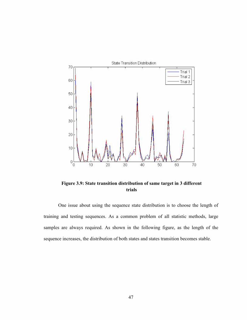
4.4 Tracking node local detection area..............................................................................65
4.5 Tracking strategies ………………………………………………………….….........66
6.1 Close set recognition rate for path dependent recognition using 2 preselected channels, data fusion, feature fusion and score fusion.................................................................73
6.2 Open set ROC curve for path dependent recognition using set 1 preselected channels
using different features................................................................................................74 6.3 Open set ROC curve for path dependent recognition using set 2 preselected channels
using different features................................................................................................75 6.4 Open set ROC curve for path dependent recognition using score fusion preselected
channels using different features.................................................................................76 6.5 Open set ROC curve for path independent recognition using set 1 preselected
channels using different features.................................................................................78 6.6 Open set ROC curve for path independent recognition using set 2 preselected
channels using different features................................................................................79 6.7 Open set ROC curve for path independent recognition with score fusion using
different features........................................................................................................80

ix
6.8 Close set recognition rate for path independent recognition using random training
scheme with 2 preselected channels, data fusion, feature fusion and score fusion..........................................................................................................................81
6.9 Snapshot of tracking one human target walking in a circle in a room. (Frame 15)….82 6.10 Snapshot of tracking one human target walking in a circle in a room. (Frame
23)…………………………………………………………………………………..83 6.11 Snapshot of tracking one human target walking in a circle in a room. (Frame
36)…………………………………………………………………………………..83 6.12 Snapshot of tracking one human target walking in a circle in a room. (Frame
42)…………………………………………………………………………………..84 6.13 Snapshot of tracking one human target walking in a circle in a room. (Frame
50)…………………………………………………………………………………..84 6.14 Snapshot of tracking one human target walking in a circle in a room. (Frame
55)…………………………………………………………………………………..85 6.15 Snapshot of tracking one human target walking in a circle in a room. (Frame
63)…………………………………………………………………………………..85 6.16 Snapshot of tracking one human target walking in a circle in a room. (Frame
68)…………………………………………………………………………………..86 7.1 Sensory data for same human target under different speed conditions……...............90
7.2 State distribution for same human target under different speed conditions ...............91
7.3 Sensory data for same human target under different cloth conditions….…................92
7.4 State transition for same human target under different cloth conditions.....................92

x
ABSTRACT
Human tracking and recognition are desirable yet challenging for many
applications including surveillance, computer vision, robotics, virtual reality, etc. Many
biometric modalities have been used on these applications. Compared to other biometric
modalities, such as fingerprints, face, and iris, gait biometrics are advantageous in their
capability of recognition at a distance under changing environmental and cosmetic
conditions. Despite having many limitations, from clothing changes to gait variation due
to different physical and emotional conditions, the discrimination power of gait can still
serve as a unique and useful component in human tracking and recognition systems.
The work presented in this thesis aims at developing a distributed wireless sensor
human recognition and tracking system, in order to improve the performance of
previously established centralized pyroelectric sensor system. Our final goal is to provide
wireless distributed pyroelectric sensor nodes as an alternative to the centralized infrared
video sensors, with lower cost, lower detectability, lower power consumption and
computation, and less privacy infringement. In previous related study, the system was
able to succeed in identifying individuals walking along the same path, or just randomly
inside a room, with an identification rate higher than 80% for around 10 subjects.
For the human recognition system, innovations and adaptations are developed in:
(1) sampling structure, multiple modified two-column sensor nodes are engaged to
leverage the ability of effective acquisition of both the shape and dynamic gait
attribution. (2) sensing protocols, different compressive measurement functions are

xi
provided for accomplishing the central task of compressive sensing protocol - choosing a
proper scheme of the random projection encoding. (3) processing architecture, different
levels of fusion schemes performed at data level, feature level, score level, and decision
level constitute the processing architecture. Along with the advent of several new digital
features, a higher recognition rate for both path dependent human recognition and path
independent human recognition is achieved. For the human tracking system, a distributed
tracking method was proposed to replace the previous centralized algorithm. Both
recognition and tracking system will eventually be combined together and work
cooperatively to form the human tracking and identification system.
Real time implementation results are presented in the thesis. Moreover,
experimental work and the related results are also discussed.

1
CHAPTER 1
INTRODUCTION
1.1 Overview
Biometric systems have been researched and tested for a few decades, but have
only recently entered into the public consciousness because of high profile applications
and increased usage by the public in day-to-day activities. [26, 45] Example deployments
within the United States Government include the FBI’s Integrated Automated Fingerprint
Identification System (IAFIS), the US-VISIT program, and the Registered Traveler
program. Many companies are also implementing biometric technologies to secure areas,
maintain time records and enhance user convenience. For example, for many years
Disney World has employed biometric devices for season ticket holder to expedite and
simplify the process of entering its parks, while ensuring that the ticket is used only by
the individual to whom it was issued.
A typical biometric system is comprised of five integrated components: 1, a
sensor is used to collect the data and convert the information to a digital format; 2, signal
processing algorithms perform quality control activities and develop the biometric
template; 3, a data storage component keeps information that new biometric templates
will be compare to; 4, a matching algorithm compares the new biometric template to one
or more templates kept in data storage; 5, a decision process uses the results from the
matching component to make a system-level decision.

2
Over the years, many biometric modalities, such as fingerprints, face, voice, iris
and gait have been studied and applied to human recognition application. Following are
some examples:
• Fingerprints have an uneven surface of ridges and valleys that form a
unique pattern for each individual. For most applications, the primary
interest is in the ridge patterns on the top joint of the finger.
• Many face recognition approaches have existed for several years using
low resolution 2D images. Recent work in high resolution 2D and 3D
shows the potential to greatly improve face recognition. Despite the
volumes of research, there are no agreed-upon methods for automated face
recognition as there are for fingerprints.
• The concept of using the iris for recognition purposes dates back to 1936.
To obtain a good image of the iris, identification systems typically
illuminate the iris with near-infrared light. A common misconception is
that iris recognition shines a laser on the eye to “scan” it. This is incorrect
untrue. Iris recognition simply takes an illuminated picture of the iris
without causing any discomfort to the individual.
• Speaker recognition uses an individual’s speech, a feature influenced by
both the physical structure of an individual’s vocal tract and the behavioral
characteristics of the individual, for recognition purposes. [36, 37, 38, 39]
3
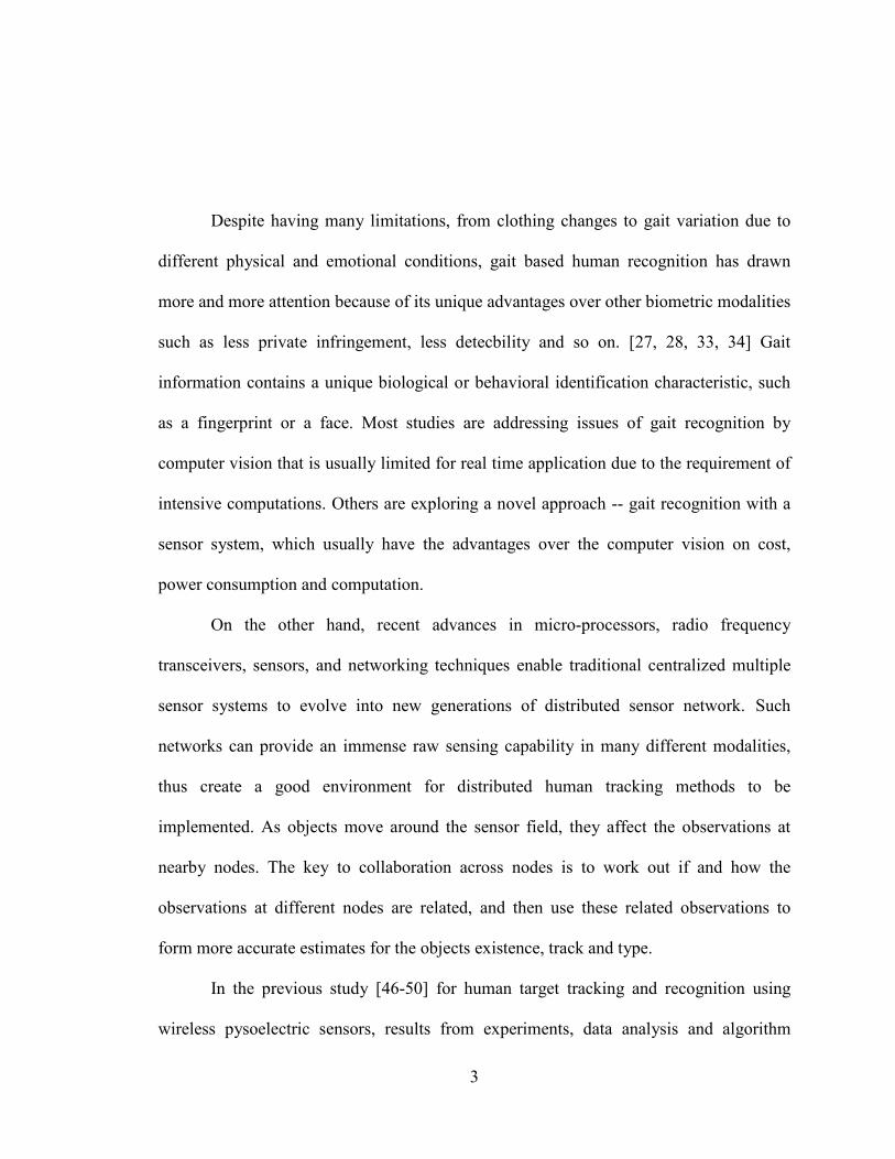
Despite having many limitations, from clothing changes to gait variation due to
different physical and emotional conditions, gait based human recognition has drawn
more and more attention because of its unique advantages over other biometric modalities
such as less private infringement, less detecbility and so on. [27, 28, 33, 34] Gait
information contains a unique biological or behavioral identification characteristic, such
as a fingerprint or a face. Most studies are addressing issues of gait recognition by
computer vision that is usually limited for real time application due to the requirement of
intensive computations. Others are exploring a novel approach -- gait recognition with a
sensor system, which usually have the advantages over the computer vision on cost,
power consumption and computation.
On the other hand, recent advances in micro-processors, radio frequency
transceivers, sensors, and networking techniques enable traditional centralized multiple
sensor systems to evolve into new generations of distributed sensor network. Such
networks can provide an immense raw sensing capability in many different modalities,
thus create a good environment for distributed human tracking methods to be
implemented. As objects move around the sensor field, they affect the observations at
nearby nodes. The key to collaboration across nodes is to work out if and how the
observations at different nodes are related, and then use these related observations to
form more accurate estimates for the objects existence, track and type.
In the previous study [46-50] for human target tracking and recognition using
wireless pysoelectric sensors, results from experiments, data analysis and algorithm
4
design are promising. The main idea is when a human walks through the visibility
modulated object space, the sensors will generate a binary signal sequence that contains
gait information as well as location information of the walker. By finding the pattern
hidden in the signal sequences, the human objects can be located and recognized. The
work presented in this thesis suggested several new methods, which improves the
performance of the human tracking and recognition system.
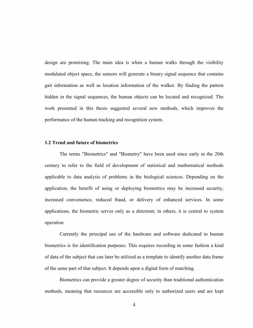
1.2 Trend and future of biometrics
The terms "Biometrics" and "Biometry" have been used since early in the 20th
century to refer to the field of development of statistical and mathematical methods
applicable to data analysis of problems in the biological sciences. Depending on the
application, the benefit of using or deploying biometrics may be increased security,
increased convenience, reduced fraud, or delivery of enhanced services. In some
applications, the biometric serves only as a deterrent; in others, it is central to system
operation.
Currently the principal use of the hardware and software dedicated to human
biometrics is for identification purposes. This requires recording in some fashion a kind
of data of the subject that can later be utilized as a template to identify another data frame
of the same part of that subject. It depends upon a digital form of matching.
Biometrics can provide a greater degree of security than traditional authentication
methods, meaning that resources are accessible only to authorized users and are kept

5
protected from unauthorized users. Traditional passwords and PINs are easily guessed or
compromised; tokens can be stolen. By contrast, biometrics data cannot be guessed or
stolen in the same fashion as a password or token. Although some biometric systems can
be broken under certain conditions, today’s biometric systems are highly unlikely to be
fooled by a picture of a face, an impression of a fingerprint, or a recording of a voice.
This assumes, of course, that the imposter has been able to gather these physiological
characteristics—unlikely in most cases. Because biometrics are difficult if not impossible
to forget, they can offer much greater convenience than systems based on remembering
multiple passwords or on keeping possession of an authentication token. For PC
applications in which a user must access multiple resources, biometrics can greatly
simplify the authentication process—the biometric replaces multiple passwords, in theory
reducing the burden on both the user and the system administrator. Applications such as
point-of-sale transactions have also begun to see the use of biometrics to authorize
purchases from prefunded accounts, eliminating the need for cards. Biometric
authentication also allows for association of higher levels of rights and privileges with a
successful authentication.
Just as leading biometric technologies differ in fundamental ways, the major
biometric applications differ substantially in terms of security and convenience
requirements, process flow of enrollment and verification, and system design.
Nowadays, biometric applications are mainly divided into just three categories:
• Applications in which biometrics provide logical access to data or information.

6
• Applications in which biometrics provide physical access to tangible materials or
to controlled areas.
• Applications in which biometrics identify or verify the identity of an individual
from a database.
In the future, behavioral and medical diagnostics will keep drawing more
attention and many promising projects will be put to application. For example, a full
home health care appliances and software are possible long range future markets, either
in modules or as complete units, probably directly interfacing with primary care
organizations. This advance could follow the clinical and institutional market saturation
of medical history and diagnostic applications. Another good example is a full
surveillance home safety system can be applied using biometric, no password or PIN is
needed. It offers residents both more reliable and convenient safety system.
1.3 Compressive human recognition
There are two topics included in the compressive human recognition:1, how to
implement data condensing while maintaining essential integrity of each individual
feature, which is also known as a problem of compressing sensing. Successful
compressing sensing scheme enable us to implement our recognition system at the
physical layer where the processing speed can be greatly improved when using MAC
layer protocol. 2, how to further keep or enhance if possible the identification/verification

7
performance, in another word, given the digital patter from different walker, we are
trying to find a stable and unique feature belongs to different individual.
To address the first problem, we tried to increase the sensing range hoping to
capture more gait information. Firstly we modified our identification node from one-
column to two-column with the visibility coding listed in Table 1.1, thus each sensor
node can hold 8 sensors as shown in Figure 1.1.
Two more such identification nodes are added to our system, and all 3 nodes are
put in 3 different positions as shown in figure 1.2. In such case, the digital data would
Fig 1.1: Identification sensor node modification

8
contain more detail information about the walker features. For example, when walking
along the fixed path 1 as the black line shown in Figure 1.2, sensor node 3 can capture the
front motion of the walker while the other two can collect the silhouette dynamics. Then
we evaluated the information quality of each bit and apply the bits with best quality for
compressive sensing. Several criterions were considered, and self-correlation and entropy
value are found to be useful for this purpose.
Table 1.1 Visibility coding scheme of the recognition node
LENS ARRAY OLD VISIBILITY LENS ARRAY NEW VISIBITILTY
1 [1 0 1 0 1 0 1 0 1 0 1] 1 [1 0 1 0 1 0 1 0 1 0 1]
2 [0 1 0 1 0 1 0 1 0 1 0] 2 [0 1 0 1 0 1 0 1 0 1 0]
3 [1 0 1 0 1 0 1 0 1 0 1] 3 [1 0 1 0 1 0 1 0 1 0 1]
4 [0 1 0 1 0 1 0 1 0 1 0] 4 [0 1 0 1 0 1 0 1 0 1 0]
5 [1 0 1 0 1 0 1 0 1 0 1]
6 [0 1 0 1 0 1 0 1 0 1 0]
7 [1 0 1 0 1 0 1 0 1 0 1]
8 [0 1 0 1 0 1 0 1 0 1 0]

9
For the second problem, we introduced compressive sensing idea to our system,
meanwhile we designed different sequence mining schemes hope to find the best
dynamic feature as well as statistic feature that can efficiently and robustly represent the
walker characters. At the same time, we continued the previous work about HMM model
and tried to use the Variational Bayesian Hidden Markov Models in our recognition
system.
1.4 Distributed human tracking
Fig 1.2: Recognition system setup
10
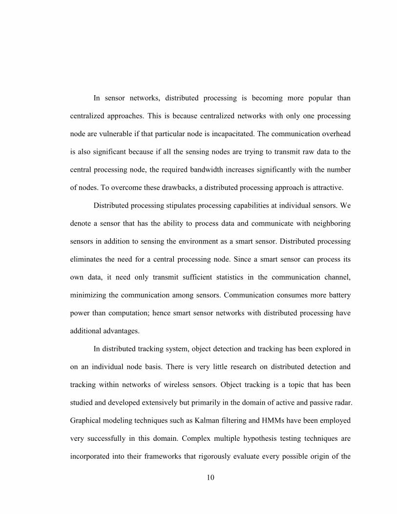
In sensor networks, distributed processing is becoming more popular than
centralized approaches. This is because centralized networks with only one processing
node are vulnerable if that particular node is incapacitated. The communication overhead
is also significant because if all the sensing nodes are trying to transmit raw data to the
central processing node, the required bandwidth increases significantly with the number
of nodes. To overcome these drawbacks, a distributed processing approach is attractive.
Distributed processing stipulates processing capabilities at individual sensors. We
denote a sensor that has the ability to process data and communicate with neighboring
sensors in addition to sensing the environment as a smart sensor. Distributed processing
eliminates the need for a central processing node. Since a smart sensor can process its
own data, it need only transmit sufficient statistics in the communication channel,
minimizing the communication among sensors. Communication consumes more battery
power than computation; hence smart sensor networks with distributed processing have
additional advantages.
In distributed tracking system, object detection and tracking has been explored in
on an individual node basis. There is very little research on distributed detection and
tracking within networks of wireless sensors. Object tracking is a topic that has been
studied and developed extensively but primarily in the domain of active and passive radar.
Graphical modeling techniques such as Kalman filtering and HMMs have been employed
very successfully in this domain. Complex multiple hypothesis testing techniques are
incorporated into their frameworks that rigorously evaluate every possible origin of the

11
measurements received. However, they assume that all the measurements are available
for processing at a centralized node. In order to develop a distributed tracking sensor
system, a generic algorithm that can be applied to the modality available is essential. The
figure below shows the sensor node deployed in the tracking system and the system setup
during the experiment.
Fig 1.3: Distributed tracking sensor node

12
Table below shows the visibility coding mask for distributed tracking sensor
node.
Table 1.2 Visibility coding scheme of distributed tracking node
LENS ARRAY VISIBITILTY
1 [0 1 1 0 0 0 0 0 0 0 0]
2 [0 0 1 1 0 0 0 0 0 0 0]
3 [0 0 0 0 1 1 0 0 0 0 0]
Fig 1.4: Distributed tracking system setup

13
4 [0 0 0 0 0 1 1 0 0 0 0]
5 [0 0 0 0 0 1 1 0 0 0 0]
6 [0 0 0 0 0 0 1 1 0 0 0]
7 [0 0 0 0 0 0 0 0 1 1 0]
8 [0 0 0 0 0 0 0 0 0 1 1]
1.5: Thesis outline
The next chapter briefly discusses preliminary knowledge, including data
recovery, compressive sensing, sequence mining, distance function and sensor model and
visibility modulation. Given these preliminary factors, based on which our research was
carried on, Chapter 3 describes the detail development of the compressive human
recognition and presents the results form of plots. Chapter 4 introduces the distributed
tracking scheme as well as implementation. The experimental setup is presented in
Chapter 5 and the results are presented in Chapter 6. Chapter 7 summarizes the work and
presents possible future direction of the work.

14
CHAPTER 2
PRELIMINARY
2.1 Introduction
This chapter discusses several issues we had during the research and the solution
as well as the backgrounds to those solutions. In Sensor model and visibility modulation,
we give a illustration about the sensor model and how the visibility modulation influence
the result of sensory data. The ideas of compressive sensing, sequence mining and
distance function are also presented here. Compressive sensing plays promising roles in
the tradeoff between the high information gain in expectation out of distributed sensor
systems and the bottleneck in reality of their narrow data throughput and limited
computation power. [41] Sequence mining is concerned with finding statistically relevant
patters between data examples where values are delivered in a sequence. In our case,
since the sensory data are presented in the form of binary sequence, it is critical for us to
explore the field of sequence mining in order to find and evaluate the patter hidden in
each sequence. Sequence distance functions are designed to measure sequence similarity.
How to evaluate similarity between sequences belong to different human target the
central idea for identification and recognition. Given the feature, the feature based
sequence distance allows us to use the measureable quantity to make the recognition
decision.

15
2.2 Sensor model and visibility modulation
In this section, we present a pyroelectric sensor system model, including sensor
node architecture, sensor visibility and its modulation by a Fresnel lens array. The design
of sensor modules is also described.
Figure 2.1 shows the architecture of the sensor node in our system. Robust
collaborative signal processing techniques can map the signal states, measured by the
distributed sensors, through low-level local computation at each node, into configuration
state sequences, which after decision fusion constitute the final identities of targets. A
suitable networking protocol guarantees reliable information routing and data
dissemination. We employed the master/slave communication mode. Once the
master/slave relationship is established, the direction of control is always from the master
to the slave(s).

16
The pyroelectric sensing circuits create the signal space, Fresnel lens arrays
produce the visibility modulation, and human thermal sources form the object space.
Under the linearity assumption, the response signal of m sensors, 𝑠𝑠(𝑡𝑡) ∈ 𝑅𝑅𝑚𝑚 is given by
𝒔𝒔(𝑡𝑡) = ℎ(𝑡𝑡) ∗ � 𝒗𝒗(𝒓𝒓)𝜓𝜓(𝒓𝒓, 𝑡𝑡)𝑑𝑑𝒓𝒓𝛺𝛺
Where “*” denotes convolution, h(t) is the impulse response of one sensor, Ω is the
object space, 𝑽𝑽(𝒓𝒓)ϵ[0,1]m is the modulated visibility function between m sensors and the
object space, ψ(r, t) is the radiation from the object.
Figure 2.1: Sensor node architecture

17
The Fresnel lens we employ is made of a light-weight, low-cost plastic material
with good transmission characteristics in the 8~10 μm range. We first utilize the Fresnel
lens array to modulate the visibility of our sensors, such that each sensor can observe
events uniformly distributed over 11 angles as shown in Figure 2.2. Coded masks are
then used to differentiate the sensors' FOVs, such that each sensor can measure different
combinations of thermal variation in space caused by motion of human subjects. The
underlying mechanism and main motivation of developing geometric sensors in
identification is the study of reference structure tomography and compressive sensing. It
suggests that multi-dimensional features of a radiation source could be captured at an
arbitrary level, once there exists a set of base functions that structurally pose and
numerically condition the reconstruction procedure, by fine tuning the multi-dimensional
visibilities of distributed sensors. Through its scan-free multi-dimensional imaging, the
feature abstraction, shape parameterization, and even characteristic classification of
radiation sources under examination can be achieved in a data-efficient and computation-
efficient way.

18
2.3 Compressive sensing
Using multiple sensor nodes described in 1.3 allows enhancing the performance
of the distributed sensor system. However, doing so also introduces huge amount noise,
redundancy as well as increases the computational complexity. In absence of compressive
sensing, one would have to directly use the 24 bits data, then the 2^24=16777216
possible states have to be calculated, which would make the implementation impossible.
Compressive sensing, also known as sparse sensing and compressive sampling, is
a technique for acquiring and reconstructing a signal utilizing the prior knowledge that it
Figure 2.2: Top and side Fresnel lens visible zone

19
is sparse or compressible. The field has existed for at least four decades, but recently the
field has exploded.
The main idea behind compressed sensing is to exploit that there is some structure
and redundancy in most interesting signals—they are not pure noise. In particular, most
signals are redundant. It plays promising roles in the tradeoff between the high
information gain in expectation out of distributed sensor systems and the bottleneck in
reality of their narrow data throughput and limited computation power.
In our system, the implementation of compressive sensing originates from the
efforts to improve data collection efficiency–one sensor can sense different type of events,
to capture main components of both motions and radiation features of human objects at
the stage of sensory data acquisition, to increase the robustness of the mapping between
measurement states of sensors and configuration states of human objects by properly
exploiting the sensor redundancy, and to achieve high data processing efficacy and
efficiency, which would allow us eventually to implement data processing in the physical
layer.
Enabled by multiplex sensing and multichannel, guided by the data evaluation
criterions, inspired by the modern compressive sensing technology, we deployed several
random compressive methods in our experiment, even thought the results might not be as
good as we expected, several interesting aspects drew our attention:
The first random compressive method is random bit data selection from selected
bits. In this case compressive sensing in our application starts with taking a randomized

20
sample in each frame from different preselected channels, bit 6, 9 and 20, respectively.
These channels are selected based on data evaluation discussed in the next chapter. Then
the result sequence which contains partial information of each of the 3 channels would be
used to form a new model for walker. To compare analyze the effect of bit random
selection compressive sensing, we replace the single channel bit data sequence with the
compressed one bit data sequence, draw the ROC curve using the same method as before.
The result is shown below.
Figure 2.3: ROC curve for bit random selection using direct data

21
From the plot, we can see that the performance of random bit selection lies
between the performance of the best individual channel and the worst individual channel.
This is because the random selection scheme is executed at each frame, the task of
maintaining essential integrity of each individual feature would involve sacrificing the
dynamic information – that is, the dynamic changes, 2nd level, 3rd level and 4th level data
transitions, that belong to individual channel might be lost due to switch between
channels. At the same time, we believe this random scheme can also reveal some hidden
feature by switch between the channels. It is like playing peg-tops with pictures on it,
Figure 2.4: ROC curve for bit random selection using transition data

22
when the peg-tops is spinning, it is actually has same effect as one constantly change the
point of view to the peg-tops, and usually the new pattern appears.
To compare with the first random compressive scheme, we introduced the second
compressive sensing method, the frame random selection compress. The difference
between this method and the previous one is the length of sample, in the bit random
selection method, we start the random selection at each frame, but here we only start
random selection after a given fixed frame length. That is, when the fixed frame length is
equal to 1, both of these methods have same effect. To see the effect of this compressive
method, we set the frame length to 40 and draw the ROC using the same method as
before.
Figure 2.5: ROC curve for frame random selection using direct data

23
From the figure, we can tell that the frame random selection method does not
bring a better effect to the result when compare with bit selection method. In this case,
the longer the frame length is set, the more individual channel pattern can be reserved.
However, when switching channels, a new channel pattern is introduced. As a result, a
sequence contains some patter of each individual but not strong enough to represent any
of them is generated. As a result the recognition ability is reduced by the frame random
selection. To verify our thoughts, we plot the ROC curve using different frame length as
shown below. We can see that as the length of the frame length is increasing, the ROC
area is reducing.
Figure 2.6: ROC curve for frame random selection using transition data

24
One problem with compressive sensing using bit random selection is the sources
should hold similar information. For example, assume there are 5 people keep talking
about the same topic using their own expression and the sixth person wants to know
about the topic but he/she is only allowed to listen to one of the 5 people at one time.
Common sense tells us that the sixth person should still be able to understand the topic
after listening for a while. However, if the 2 of 3 of the 5 people only talk occasionally,
then the sixth person will have to listen more in order to understand the topic. In our
system, due to the assigned location differences, few sensors rarely collect the
information. Using these channels will no longer maintain the integrity of the target
Figure 2.7: ROC curve frame using random selection with different frame length

25
information. That is why we introduced data evaluation in the next chapter to guarantee
the reliability of channels.
2.4 Sequence mining
Sequence mining is concerned with finding statistically relevant patters between
data examples where values are delivered in a sequence. Roughly speaking, a sequence
pattern consists of a number of single-position patterns plus some inter-positional
constrains. A single position pattern is essentially a condition on the underlying element
type. A sequence pattern may contain zero, one, or multiple single-position patterns. For
each position, where the single-position patterns for a given position are perhaps
associated with a probability distribution; inter-position constraints specify certain linkage
between positions; such linkage can include conditions on position distance and perhaps
also include transition probabilities from position to position when two or more single-
position patterns are present for some position.
Sequence pattern, also referred as sequence features, can be considered along the
following perspectives:
Explicit versus implicit: some features are patterns that occur in the sequence
while others are constructed from properties of the sequences or objects underlying the
sequences.
Presence versus count: A pattern can generate two types of features. In the first,
one uses the pattern as a Boolean feature, by simply considering the presence/absence of

26
the pattern in the sequence. In the second, one uses the pattern as a numerical feature, by
considering the count of the pattern in the sequence.
Frequency based feature selection: the features with high frequencies namely those
having frequency over a given threshold, are selected.
Discrimination based feature selection: features with relatively higher frequency at
a desired site or in some selected classes than elsewhere are preferred. To find features for
identifying a desired site, one prefers features which occurs quire frequently around the
site than elsewhere.
2.5 Distance function
Sequence distance functions are designed to measure sequence similarities.
Roughly speaking, distance functions can be character based, feature based, and
information theoretic based, conditional probability distribution etc. In feature based
approach, one would first extract features from the sequences, and then compute the
distance between the sequences by computing the distance between the feature vectors of
the sequences.
There are several distance functions for sequence. The edit distance, also called
Levenshtein distance, between two sequences S1 and S2, is defined to be the minimum
number of edit operations to transform S1 to S2. The edit operations include changing a
letter to another, inserting a letter and deleting a letter. The hamming distance between
two sequences is limited to cases when the two sequences have identical lengths, and is

27
defined to be the number of positions where the two sequences are different. For
conditional probability distribution based distance, the idea is to use the CPD of the next
symbol to characterize the structural properties of a given sequence. The distance
between two sequences is then defined in terms of the difference between the two CPDs
of the two sequences. The similarity between two CPDs can be measure by the
variational distance or the Kullback-Leibler divergence between the CPDs. In probability
theory and information theory, the Kullback–Leibler divergence (also information
divergence, information gain, or relative entropy) is a non-commutative measure of the
difference between two probability distributions P and Q. KL measures the expected
number of extra bits required to code samples from P when using a code based on Q,
rather than using a code based on P. Typically P represents the "true" distribution of data,
observations, or a precise calculated theoretical distribution. The measure Q typically
represents a theory, model, description, or approximation of P. It is a special case of a
broader class of divergences called f-divergences. Although it is often intuited as a
distance metric, the KL divergence is not a true metric since it is not symmetric (hence
'divergence' rather than 'distance') and does not satisfy the triangle inequality. For
probability distributions P and Q of a discrete random variable the K–L divergence of Q
from P is defined to be
𝐷𝐷𝐾𝐾𝐾𝐾(𝑃𝑃||𝑄𝑄) = �𝑃𝑃(𝑖𝑖)𝑖𝑖
𝑙𝑙𝑙𝑙𝑙𝑙𝑃𝑃(𝑖𝑖)𝑄𝑄(𝑖𝑖)

28
CHAPTER 3
COMPRESSIVE HUMAN RECOGNITION
3.1 Introduction
Identity recognition is becoming increasingly important in many applications
including access control and e-commerce. Current approaches for identity recognition are
based on passcards or PIN numbers that can be stolen or forgotten. The use of biometrics
(e.g., face, fingerprints, voice patterns, palmprints, iris images, etc.) will improve
security, since biometrics is integral to a person. Recognition includes verification
(authenticating or rejecting a claimed identity) and identification (matching a presented
biometric to one of several in a database). Over the past decade, significant advances
have been made in biometric recognition.
In this chapter, the compressive human recognition is introduced. But before we
continue to the detail, there are several important concepts of the human recognition need
to be addressed.
The human recognition can be performed in two ways:
1) Closed-Set Walker Identification.
The automatic system must determine who is walking. The condition for the
system to work correctly is that the walker belongs to a predefined set of known walkers.
However, if the set of known walkers do not cover the current target, the system will not

29
be able to give the correct result. The system performance is evaluated using
identification rate.
2) Open-Set Walker Identification.
Open Set operates under the assumption that not all the test probes have mates in
the gallery. It either detects the presence of some biometric signature within the gallery
and finds its identity or rejects it, i.e., it can provide for the "none of the above” answer.
In this approach, the system accepts or rejects the users according to a successful or
unsuccessful verification. Sometimes this operation mode is also called as verification or
authentication. The system performance is evaluated using the False Acceptance Rate
(FAR, those situations where an impostor is accepted) and the False Rejection Rate
(FRR, those situations where a walker is incorrectly rejected), also known in detection
theory as False Alarm and Miss, respectively. This framework gives us the possibility of
distinguishing between the discriminability of the system and the decision bias. The
performance can be plotted in a Receiver Operator Characteristic (ROC) plot, where the
Detection Rate (DR = 1-FRR) is instead used in most cases.
Despite the different requirements of open-set and closed-set walker
identification, they are intrinsically related to one another. For an open-set identification
system, the optimal decision threshold has to be obtained from the ROC curves generated
from verification testing results. For the verification problem, the unknown walker’s data
sample is compared to the database. If the claimed walker is among the best matches, the

30
walker is accepted and otherwise rejected. In both cases (identification and verification),
walker recognition techniques can be split into two main modalities:
1) Path Independent.
This is the general case, where the system does not know the path walked by the
person. This operation mode is mandatory for those applications where the user does not
know that he/she is being evaluated. This allows more flexibility, but it also increases the
difficulty of the problem. From the signal processing viewpoint, one must extract a
specific statistical pattern for each person.
2) Path Dependent.
This operation mode implies that the same path is taken by everyone. The
recognition relies on the comparison of the measured signals. Given that the response
signals are usually speed dependent, there are two solutions. Our objective is to develop
features that are less sensitive to the speed. This mode is useful for those applications
with strong control over user input similar to its text dependent speaker recognition
counterpart.
This chapter describes the compressive human recognition, which includes: event
and feature, recognition strategies, data evaluation, digital feature extraction and fusion
scheme.
3.2 Event and feature

31
An event could be defined as an occurrence of interest in spatial-temporal space
distinguishable from its environment and repeatable in multiple trials. In our case, as
shown in figure 3.1, it is an instance in which the thermal flux collected by a pyroelectric
sensor is above a threshold and its response data can be associated with one or several
specific human motions, such as moving across one detection region.
Features are the individual measurable heuristic properties of the phenomena
being observed. Choosing discriminating features is key to any pattern recognition
algorithm being successful in classification. Two kinds of features can be extracted from
pyroelectric sensor (array) signals, the binary event index sequence of a sensor array and
the spectral segment of the data of one event. The first one is defined as the digital feature;
the second one as the analog feature. We focus on the former one, which are extracted
from event indexes sequences.
Both the event and feature are defined in the pyroelectric signal space. Signal
processing techniques such as Kalman filtering, FFT, and band-pass sine filtering are
proposed to detect the events embedded in the sensory data.

32
3.3 Recognition strategies
Given the definition of event and feature, the identification strategy for the
distributed sensors, as shown in Figure 5, includes: event detection; event data acquisition,
to acquire the data inside a event window after that event is validated; feature extraction,
to extract the feature out of the event data based on the predefined feature-to-event
association; membership estimation, to estimate the membership of one feature with
respect to all the feature models of enrolled individuals; and object identification, to make
Figure 3.1: Illustration of motion detection by the pyroelectric sensor

33
a decision on the identity of the human object under testing according to the estimated
membership likelihood vector and the inference rule.
3.4 Data evaluation
Due to different signal response and spatial location of each sensor, the event
extracted from the sensors varies. Some sensors might contain more useful information
while others might introduce noise. Data evaluation is an indispensible step which helps
us to tell the two apart, thus improve the performance of our system. Our goal is to obtain
credible information that can correctly represent the walker’s gait signature. Being
credible here consists of two elements: repeatability and uniqueness. Repeatability is the
variation in measurements taken by the sensor nodes on the same walker and under the
same conditions. A measurement may be said to be repeatable when this variation is
smaller than some agreed limit. Especially for fix path walker recognition, since target
walker walks along the same path back and forth, so we should expect to capture the
period signal that can at least depict this dynamic procedure. Uniqueness can be regards
Figure 3.2: General recognition scheme for distributed pyroelectric sensors
34
as the phrase "there is one and only one", which is used to indicate that exactly one object
with a certain property exists.
Given the collected data, how to decide if the data contains sufficient information,
how to tell if this sequence data is repeatable, is there any uniqueness contained in the
data? The answers to these questions are essential to improve the system performance. To
answer the above issues, we investigated two traditional signal-processing approaches:
entropy analyzes and self-correlation analyze.
Entropy has often been loosely associated with the amount of order, disorder,
and/or chaos in a thermodynamic system. We use entropy to evaluate the repeatability of
the data. The traditional qualitative description of entropy is that it refers to changes in
the status quo of the system and is a measure of "molecular disorder" and the amount of
wasted energy in a dynamical energy transformation from one state or form to another.
The definition of entropy is given by the following equation:
𝑆𝑆 = −�𝑃𝑃𝑖𝑖𝑙𝑙𝑙𝑙𝑃𝑃𝑖𝑖𝑖𝑖
where S is the conventional symbol for entropy. The sum runs over all microstates
consistent with the given macro-state and 𝑃𝑃𝑖𝑖 is the probability of the ith microstate. For
each bit data, we evaluate the 1st, 2nd, 3rd and 4th level data transition entropy. They are
defined as below:
1st level data transition has only two states: ‘0’ and ‘1’. It represents the spatial
occurrences state when a walker passes through.

35
2nd level data transition has four states: ‘00’, ’01’,’10’, and ’11’. It contains the 1st order
dynamic transition information as the walker pass by in certain spatial area.
3rd level data transition has 8 states: ‘000’, ’001’, ’010’, ’011’, ’100’, ’101’, ’110’, and
’111’. It contains the 1.5nd order dynamic transition information.
4th level data transition has 16 states: ‘0000’, ’0001’, ’0010’, ’0011’, ’0100’, ’0101’,
’0110’, ’0111’, ’1000’, ’1001’, ’1010’, ’1011’, ’1100’, ’1101’, ’1110’ and ‘1111’. It has
the 2nd order dynamic character.
So given the 24 bits data as shown in the figure below, the entropy can be calculated as
listed in table 2.
Figure 3.3: 1000 frame 24 bits data collected by the sensors

36
Table 3.1 Different level of entropy for binary data in Figure 3.3
BIT INDEX 1st LEVEL 2nd LEVEL 3rd LEVEL 4th LEVEL
1 0.8127 1.4152 1.9823 2.5412
2 0.6406 1.0899 1.5071 1.9226
3 0.7531 1.2701 1.7448 2.2126
4 0.8825 1.5165 2.1047 2.6822
5 0.9111 1.4715 1.9921 2.4975
6 0.9986 1.7419 2.4229 3.0931
7 0.2799 0.4741 .6587 .8391
8 0.4817 0.8188 1.1384 1.4526
9 0.9448 1.6230 2.2466 2.8589
10 0.9271 1.6248 2.3092 2.9757
11 0.9990 1.7001 2.3786 3.0537
12 0.9100 1.5503 2.1547 2.7488
13 0.8105 1.2626 1.6915 2.1170
14 0.9991 1.7066 2.3490 2.9755
15 0.9926 1.7149 2.4160 3.1068
16 0.8468 1.3290 1.7867 2.2382
17 0.2970 0.5173 0.7347 0.9511
18 0.7055 1.2419 1.7615 2.2772

37
19 0.5063 0.8638 1.2031 1.5398
20 0.9901 1.7988 2.5698 3.3329
21 0 0 0 0
22 0.2533 0.4181 0.5794 0.7358
23 0.7219 1.2789 1.7837 2.2781
24 0.5932 0.9787 1.3481 1.7106
If we sort the bit index according to 5 different entropy criterions, we can get 5
similar sorting results. To get the results without losing the general information, we use
the summation of all 5 entropy values for evaluating the bit data repeatability, bit 21, 7, 8,
24 and13 are among the bits with small entropy value, it is obvious that the binary data of
these bits contain high periodicity. Thus we believe this could be a very way to find the
repeatability of sensor data. Notice that bit 21 does not have any value for the walker so
we assign 0 for its entropy.
Self-correlation, also known as Autocorrelation, is a mathematical tool for finding
repeating patterns, such as the presence of a periodic signal which has been buried under
noise, or identifying the missing fundamental frequency in a signal implied by its
harmonic frequencies. However, we used self-correlation as a method to find out if the
sensor data is unique. Based on the strong assumption that the uniqueness should be lying
under the intricate dynamic process, the more transition the bit data has, the more likely it
contains the uniqueness with respect to the individual walker. So the idea is to calculate

38
the self-correlation of the distribution of the 4th level data transition; we can expect to see
more peaks in results if the distribution contains more dynamic transitions. As a result, it
will also increase the area the self-correlation result plot covers. Here is the result based
on the same data image presented in figure 3.3.

39
Figure 3.4: Self-correlation of 24 bits data in figure 3.3

40
We can see that bit 21, which has very low entropy value, also has very low self-
correlation area. It will not get a positive evaluation after this step.
Using the above evaluation approaches, one bit was chosen from each sensor
node, bit 6, 9 and 20 respectively. To assess the evaluation results, we collected the data
from 5 different walker and implemented the closed set recognition test using both 1 bit
direct data and 1 bit transition data with KL Distance feature. (The feature extraction will
be discussed later) 2 ROC curves were generated as shown below:
Figure 3.5: ROC curve for single bit 6, 9 and 20 using direct data
41
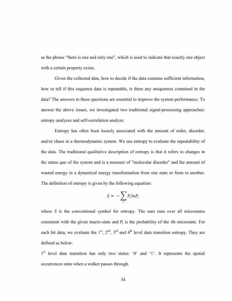
Results show us that each of the three bits has individual discriminate ability. To
compare, we also plot the bit ROC using transition data for bit 1, 2 and 4. It is clear that
these 3 bits has less ROC area than the previous 3 bits.
Figure 3.6: ROC curve for single bit 6, 9 and 20 using transition data

42
In conclusion, the two approaches: entropy and self-correlation will help us find
out the bit data that contains ample transitions while maintain periodicity, hence evaluate
the data quality before compressive sensing or feature extraction.
3.5 Digital feature extraction
Any functional feature in recognition should be characterized by its universality
over all objects under testing, distinctiveness between any two individuals, invariance
over a period of time, and feasibility for quantitative measures. As mentioned early, there
Figure 3.7: ROC curve for single bit 1, 2 and 4 using transition data

43
are two types of features: the spectral vectors gathered from the analog event data and the
digital event sequences produced as a walker crossed individual beams in the modulated
object space. In our research, we only focus on digital event sequence, upon which our
walker recognition algorithms were based. Our study on pyroelectric signal feature is
chosen as statistical characterization of digital event index sequences.
In general, digitalized features should be very simple, easy to compute, and robust
to background noise, so that walker recognition detection can take place in real time and
perform well. According to the system setup as described in figure 1.2, figure 3.3
illustrates event index sequences transmitted by four wireless sensor nodes, with the
visibility codes in Table 1, when one human subject walks along fix path 1 inside a room.
With the help of data evaluation, we can choose one bit channel that can best maintain
repeatability and uniqueness of the walker from each of the 3 sensor nodes, thus leave us
with 3 bits data. To find the measurable heuristic properties hidden in the sequence, we
have to extract the sequences using sequence mining methods.
The heuristic properties hidden in the sequence can be also referred as sequence
pattern. A sequence pattern is a finite set of single-position patterns of the form {𝑐𝑐1,
…,𝑐𝑐𝑘𝑘}, together with a description of the positional distance relationships on the 𝑐𝑐𝑖𝑖’s and
some other optional specifications. Roughly speaking, a sequence pattern consists of a
number of single-position patterns plus some inter-positional constrains. A single
position pattern is essentially a condition on the underlying element type. A sequence
pattern may contain zero, one, or multiple single-position patterns. For each position,

44
where the single-position patterns for a given position are perhaps associated with a
probability distribution; inter-position constraints specify certain linkage between
positions; such linkage can include conditions on position distance and perhaps also
include transition probabilities from position to position when two or more single-
position patterns are present for some position.
The first representative sequence pattern type is the frequent sequence patterns.
Each such a pattern consists of one single-position pattern for each position. Frequent
sequence patterns can be viewed as periodic sequence patterns. In our research this type
sequence pattern can be regard as the shape information of each walker, it is one of the
static features generated according the walker’s thermal distribution.
The second representative sequence pattern type is the sequence profile patterns.
Such a pattern is over a set of positions, and it consists of a set of single-position pattern
plus a probability distribution. Here we can think of this type of pattern as the dynamic
feature produced by the walker’s walking habit.
The third representative sequence pattern type is Markov models. Such a model
consists of a number of states plus probabilistic transitions between states. In some cases
each state is also associated with a symbol emission probability distribution. This is the
feature used in our previous work, specifically Hidden Markov Model.
In an effort to build the stable and unique statistical feature model with respect to
each individual, we analyzed the digital event sequence in the following perspectives:
Explicit versus implicit, some features are patterns that occur in the sequence while

45
others are constructed from properties of the sequences or objects underlying the
sequences. Presence versus count: A pattern can generate two types of features. In the
first, one uses the pattern as a Boolean feature, by simply considering the
presence/absence of the pattern in the sequence. In the second, one uses the pattern as a
numerical feature, by considering the count of the pattern in the sequence. Frequency
based feature selection: the features with high frequencies namely those having frequency
over a given threshold, are selected.
We took the following steps to find and evaluate the feature:
1, Understand the data.
2, Preprocessing of the data with feature selection and feature construction.
Feature selection is concerned with selecting the more useful features from a large
number of candidate features. Feature construction is about producing new features from
existing features.
3, mine the patterns.
4, evaluate mining results. In this step various measures to evaluate the patterns,
mainly focusing on repeatable and uniqueness.
Several features were considered and two of these features appear to work very
well with the sensor event sequence: States Distribution and Most frequent States. As
stated earlier, the data sequence captured by the sensors with the visibility codes in Table
1, is associated with one or several specific human motions. The distribution of the states
contained in the sequence can represent certain characters of the walker such as the

46
height of the walker, the arm span when the walker walks, and so on. For example, tall
people tend to trigger certain spatial areas that short people could not reach; walkers with
big arm span would trigger more spatial areas than those who don’t swing arms when
they walk. By looking into the distribution of different states in the sequence, we can get
the information about the walker figure, usually also regarded as shape. When
considering the distribution of state transition in the sequence, we can get the information
about the dynamic of the walker’s walking habit. The figure below shows us the
distribution of both state and state transition of the same walker using 3 preselected
channels in different 3 trials.
Figure 3.8: State distribution of same target in 3 different trials
47
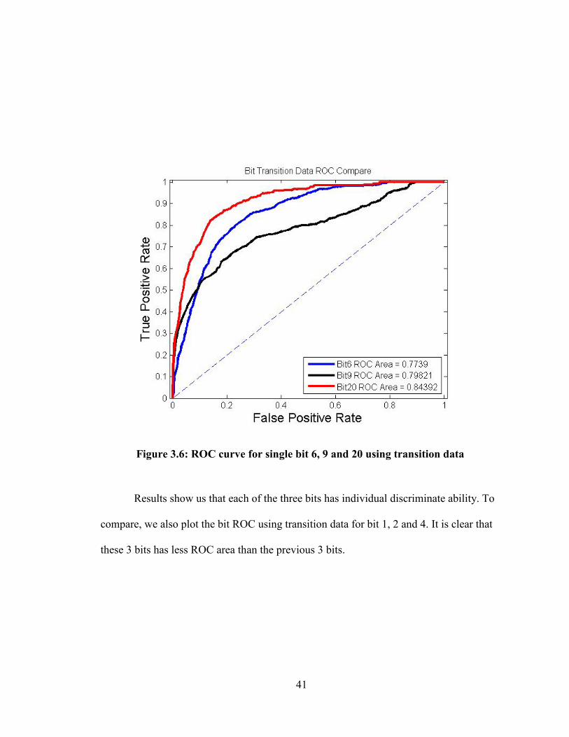
One issue about using the sequence state distribution is to choose the length of
training and testing sequences. As a common problem of all statistic methods, large
samples are always required. As shown in the following figure, as the length of the
sequence increases, the distribution of both states and states transition becomes stable.
Figure 3.9: State transition distribution of same target in 3 different trials

48
Figure 3.10: The distribution of states in 5 test sample with length 100,200,300,400 and 500 respectively.

49
Figure 3.11: The distribution of states transitions in 5 test sample with length 100,200,300,400 and 500 respectively.

50
This is a big challenge when we want to implement walker recognition in real
time. To collect enough data for a stable recognition test, the walker usually need to walk
at least for 30 seconds, which make this method less applicable. That is why we introduce
the second feature: Most frequent States. Based on the same idea as using distribution, we
want to reduce the differences between the samples due to the accident movement of
walker and noise, which would be represented by some rare seen states of the walker in
the state sequence. What we did is we do not take those signals into account for the
distribution, doing so would leave us with the most frequent states; we call it most
frequent states. In the test, we consider the 10 most frequently frequent states. Despite the
difference between the order of the most frequent states, we found this to be a stable
feature belongs to different individuals. The following table shows us the index of the 10
most frequent states of 3 different walkers. We can see that it does not change too much
with respect to different individual in 7 different tests using preselected 3 channels data
sequence.
Table 3.2 The similarity feature of 3 different targets in 7 tests
Test 1 Feature Matrix:
Target 1: 1 22 43 32 11 24 3 19 38 2
Target 2: 1 43 22 64 5 38 3 19 27 62
Target 3: 1 32 4 29 8 57 64 2 3 5
Test 2 Feature Matrix:

51
Target 1: 1 22 43 3 19 2 32 10 11 5
Target 2: 1 43 5 19 3 64 38 41 22 24
Target 3: 1 32 4 29 64 8 57 2 3 5
Test 3 Feature Matrix:
Target 1: 1 22 43 3 19 11 5 38 2 24
Target 2: 1 43 5 19 3 64 38 41 22 24
Target 3: 1 32 4 29 64 8 57 2 3 5
Test 4 Feature Matrix:
Target 1: 1 22 43 3 2 10 19 38 64 11
Target 2: 1 43 5 3 19 22 38 64 41 2
Target 3: 1 32 4 29 64 8 57 2 3 5
Test 5 Feature Matrix:
Target 1: 1 43 22 32 11 3 24 2 19 38
Target 2: 1 22 64 5 38 43 3 19 62 11
Target 3: 1 32 4 29 8 57 64 2 3 5
Test 6 Feature Matrix:
Target 1: 1 19 55 37 17 3 21 10 11 23
Target 2: 1 38 19 17 3 34 5 21 54 56
Target 3: 1 32 4 29 64 8 57 2 3 5
Test 7 Feature Matrix:

52
Target 1: 1 19 57 38 17 3 10 11 21 24
Target 2: 1 43 22 64 5 38 3 19 46 62
Target 3: 1 32 4 29 16 64 2 8 15 57
3.6 Fusion scheme
To improve the identification performance, we applied four sensor fusion
schemes, namely data fusion, feature fusion, score fusion, and decision fusion, to each
channel. Feature extraction is used to describe the most important information of the
sample data. Matching modules compares features with templates in the database and
output a score to the decision module.
Figure 3.12: Data level fusion

53
Figure 3.13: Feature level fusion
Figure 3.14: Score level fusion

54
Data level fusion combines multiple sample data sets into a single sample data set.
Feature level fusion relies on building a global statistical feature model. Score level
fusion combines scores from matching modules, and only one score is outputted to the
decision module. Decision level fusion combines decision from decision modules for
different nodes using AND, OR, or majority voting.
Figure 3.15: Decision level fusion

55
CHAPTER 4
DISTRIBUTED HUMAN TRACKING
4.1 Introduction
The emerging technology of wireless sensor networks provides many exciting and
interesting applications. Such networks can provide an immense raw sensing capability in
many different modalities. The huge difficulty in harnessing these networks lies in trying
to process all the sensed data in a meaningful and power-efficient manner. Many studies
have been put to solve this problem; one of them is distributed processing in sensor
network.
In sensor networks, distributed processing is becoming more popular than
centralized approaches. This is because centralized networks with only one processing
node are vulnerable if that particular node is incapacitated. The communication overhead
is also significant because if all the sensing nodes are trying to transmit raw data to the
central processing node, the required bandwidth increases significantly with the number
of nodes. To overcome these drawbacks, a distributed processing approach is attractive. .
The problem of object detection and tracking has been explored in on an
individual node basis. There is very little research on distributed detection and tracking
within networks of wireless sensors. Object tracking is a topic that has been studied and
developed extensively but primarily in the domain of active and passive radar. Graphical

56
modeling techniques such as Kalman filtering and HMMs have been employed very
successfully in this domain. Complex multiple hypothesis testing techniques are
incorporated into their frameworks that rigorously evaluate every possible origin of the
measurements received. However, they assume that all the measurements are available
for processing at a centralized node. Distributed processing stipulates processing
capabilities at individual sensors. [2, 3, 8, 9, 10, 11, 12, 13, 15, 16]
We denote a sensor that has the ability to process data and communicate with
neighboring sensors in addition to sensing the environment as a smart sensor. Distributed
processing eliminates the need for a central processing node. Since a smart sensor can
process its own data, it need only transmit sufficient statistics in the communication
channel, minimizing the communication among sensors. Communication consumes more
battery power than computation; hence smart sensor networks with distributed processing
have additional advantages.
Here we will outline some key design criteria for our designed distributed
tracking algorithms in the domain of wireless sensor networks:
1. Decentralized processing - While it is easier to consider and design algorithms in an
architecture where the sensor outputs are communicated back to a central processing unit,
this is generally not feasible. When dealing with a network of un-tethered nodes, a finite
amount of energy is a factor that must be taken into consideration. Communication is the
primary energy consumer. The key is to process the sensor outputs as much as possible

57
within the network, so as to avoid communicating large amounts of information over
large distances.
2. Processing sensed data at the nodes - There are many levels in which the sensed data
can be shared and processed among nodes- e.g. signal level, feature level and decision
level. At each of these levels, the information content is reduced, but this in turn reduces
the required amount of data to be communicated between nodes. In short, processing is
cheap and communication is expensive.
3. Dealing with uncertainty - Typically, the nodes are typically very low-cost, low-
power throwaway devices that might be prone to noise, increasing the chance of false
measurements. A method of estimated the data loss and data recovery is required for
robust distributed human tracking application
4. Generic algorithms for different modalities - Nodes might be equipped to record
signals from many different modalities. These might include acoustic, optical, IR,
temperature, radioactive or seismic modalities. Devising a generic algorithm that can be
applied to the modality available is preferred.
4.2 Data recovery
Data missing is a common phenomenon in wireless transmission; it could cause
huge impact on applications such as distributed tracking, where the results strongly relies
on continuous trustworthy data. For most application in wireless network, how to prevent
data loss and how to retrieve the lost data has been a long coming challenge. Usually the

58
application layer generates the data to be sent over the network and processes the
corresponding data received over the network.
One of the issues we discovered when testing our system is the data robustness.
While the experiment was conducted under very controlled circumstances, in a real
application many detected events unrelated to moving objects might occur. These false
events might be due to background phenomena, other types of objects not of interest or
perhaps faulty sensors. Data corruptions are often observed especially for tracking
system. Since tracking is a sequential process, regardless the robustness of tracking
algorithm, several lost data frames might cause the tracking to be interrupted, thus cause
the results wrong. Principle causes of the problem may be characterized into two
categories: Detector malfunction and data transmission failure between the slave and
master node. Since we deployed robust transmission protocol for our transmission, the
problem is mostly caused by the first case.
The following diagram illustrates our data recovery scheme, which mainly
contains two parts: data lost detection and data reconstruction.

59
A simple data reconstruction method using interpolation has been implemented to
replace missing or invalid data. Figure 2.2 shows the sensor collected data before and
after data recovery.
Figure 4.1: Data recovery flowchart

60
4.3 Tracking strategies
In our distributed tracking design, as shown in the figure below, The sensor
network consists of 4 sensing nodes of one modality that have a finite sensing radius due
to signal attenuation. Objects will pass through the sensor field, which is indicated by the
red line.
Figure 4.2: Sensor data before and after data recovery

61
In previous study, when sensor detect a target moving and generate events, they
are report back each event to a distant central node, it would be logical to share the
evidence among neighboring nodes and then report any useful results with the central
node. If several correlated events are associated together, a more accurate hypothesis as
to whether the object is present can be formed, along with an increasingly accurate
estimate of its position and velocity. This idea implicitly performs distributed tracking
and can be extended to that application.
It can be implemented in such way: each sensor’s local observation to produce
sensor measurements, and then communicates to the assigned local processors, the local
processors compute track estimates and transmit results to the neighbor sensor
-10 -8 -6 -4 -2 0 2 4 6 8 10
-10
-8
-6
-4
-2
0
2
4
6
8
10
Figure 4.3: Tracking system setup

62
processors, and the global fuser merges the local estimates to provide a single global
estimate of the targets to be tracked. Track-to-track fusion is an important issue in multi-
sensor data fusion. Regardless the independent measurement errors of each sensor node,
due to the correlation of sensor node, the tracking results could be greatly impacted by
noise. Figure below shows the local detection area of each node. Each local detection
area is divided into 16 grids, and different sensor data pair is mapped into one of this 16
grids. Table 4.1 shows the index of the 16 grids to the left side of the sensor. Table 4.2
shows the index of the 16 grids to the left side of the sensor. Table 4.3 and Table 4.4 give
the mapping function between the pair sensor data and its result grid index.
Table 4.1 The grid index in the left local detection area of sensor node
1 2 3 4
5 6 7 8
9 10 11 12
13 14 15 16
Table 4.2 The grid index in the right local detection area of sensor node
4 8 12 16
3 7 11 15
2 6 10 14
1 5 9 13

63
Table 4.3 The data grid index look up table for the left local detection area
Sensor Data Grid Index
0001
0010
0011
0100
0101
0110
0111
1000
1001
1010
1011
1100
1101
1110
1111
3 4 7 8 12 16
2 3 6 7 11 12
3 6 7 4 12 16
1 5 6 10 11 15
6 10 11 4 8 12
2 5 6 7 10 11
2 3 7 11 12 16
9 10 13 14 15 16
4 8 12 13 14 15
2 7 11 9 14 15
3 7 8 11 9 14
9 10 13 6 15 14
9 10 11 14 3 8
5 10 9 13 11 14
3 7 8 9 10 14

64
Table 4.4 The data grid index look up table for the right local detection area
Sensor Data Grid Index
0001
0010
0011
0100
0101
0110
0111
1000
1001
1010
1011
1100
1101
1110
1111
1 5 9 13 14
5 6 10 11 15 16
1 5 9 14 11 13
6 7 12 10 11 14
5 6 7 9 12 14
10 7 14 11 12 15
14 6 7 10 11 13
1 2 3 4 7 8
2 3 4 5 13
2 3 4 6 11 14
3 6 8 9 10 14
2 3 4 6 8 11
2 3 7 8 10 11
1 2 6 7 8 12
2 4 7 10 13 15
65
Figure 4.4 shows the tracking strategies of distributed tracking scheme. For each sensor,
it only contains the information
Figure 4.4: Tracking node local detection area
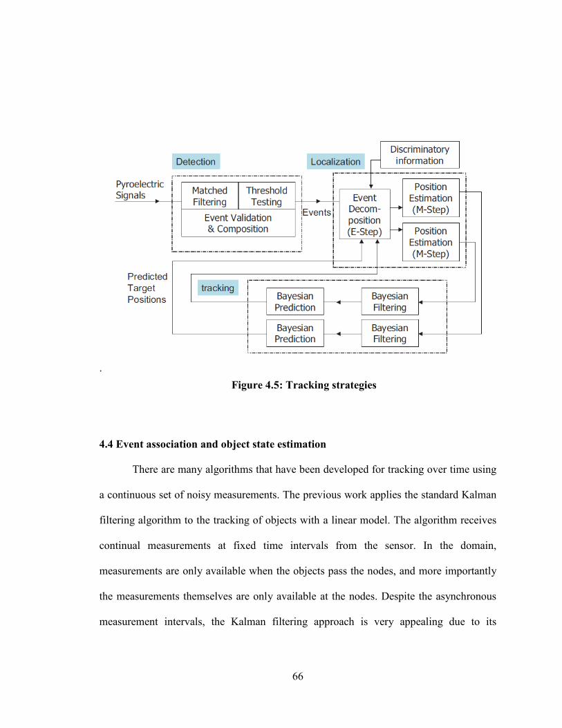
66
.
4.4 Event association and object state estimation
There are many algorithms that have been developed for tracking over time using
a continuous set of noisy measurements. The previous work applies the standard Kalman
filtering algorithm to the tracking of objects with a linear model. The algorithm receives
continual measurements at fixed time intervals from the sensor. In the domain,
measurements are only available when the objects pass the nodes, and more importantly
the measurements themselves are only available at the nodes. Despite the asynchronous
measurement intervals, the Kalman filtering approach is very appealing due to its
Figure 4.5: Tracking strategies

67
sequential convergence properties and the ‘prediction step’ that provides a means for
associating new measurements.
4.5 Distributed event association and object estimation
A distributed detection algorithm is proposed that operates as follows. Whenever
an event occurs at a node in the network, it carries out the following algorithm:
1. Check if the event occurs within the prediction gates of any previous ‘time-updated’
hypotheses received from the surrounding nodes.
2. Check if the convergence criterion is met. If so, report the confirmed object to the
central node. A distributed tracking algorithm takes over at this point.
3. Initiate a new hypothesis starting at this event
4. Broadcast the hypotheses to the surrounding nodes
In the proposed algorithm, the processing that occurs at each node in the sequence when
an event occurs is outlined.
68
CHAPTER 5
SYSTEM IMPLEMENTATION
Both the recognition and tracking wireless sensor systems are based on TI's
micro-controller and RF transceiver combination of MSP430149 and TRF6901. The
tracking system consists of one host, one master, four slave tracking slave node, while the
recognition system consists of one host, one master and three slave recognition slave
node. We use the combination of TRF6901 and MSP430149 as the computation and
communication platform. Each slave node containing pyroelectric sensors and Fresnel
lens arrays, employs an amplifier board that amplifies eight channel signals in the
frequency band 1~10 Hz. Each MSP43019 contains an 8-channel, 12-bit A/D converter,
whose sampling rate is set as 19.5 KHz, conversion rate as 96 KHz, with 5 MHz internal
ADC clock. One data package for an event includes 48 bits, i.e. 6 bytes. It means that the
sampling rate of wireless sensor system, from 10 to 80 Hz in terms of events, is virtually
determined by the embedded computation time. The TRF6901 is an integrated circuit
intended for use as a low cost FSK or OOK transceiver to establish a frequency-
programmable, half-duplex, bidirectional RF link. The multichannel FM transceiver is
intended for digital (FSK, OOK) modulated applications in the new 868-MHz European
band and the North American 915-MHz ISM band. The single-chip transceiver operates
down to 1.8 V and is designed for low power consumption. The synthesizer has a typical
channel spacing of approximately 200 kHz and uses a fully-integrated VCO.
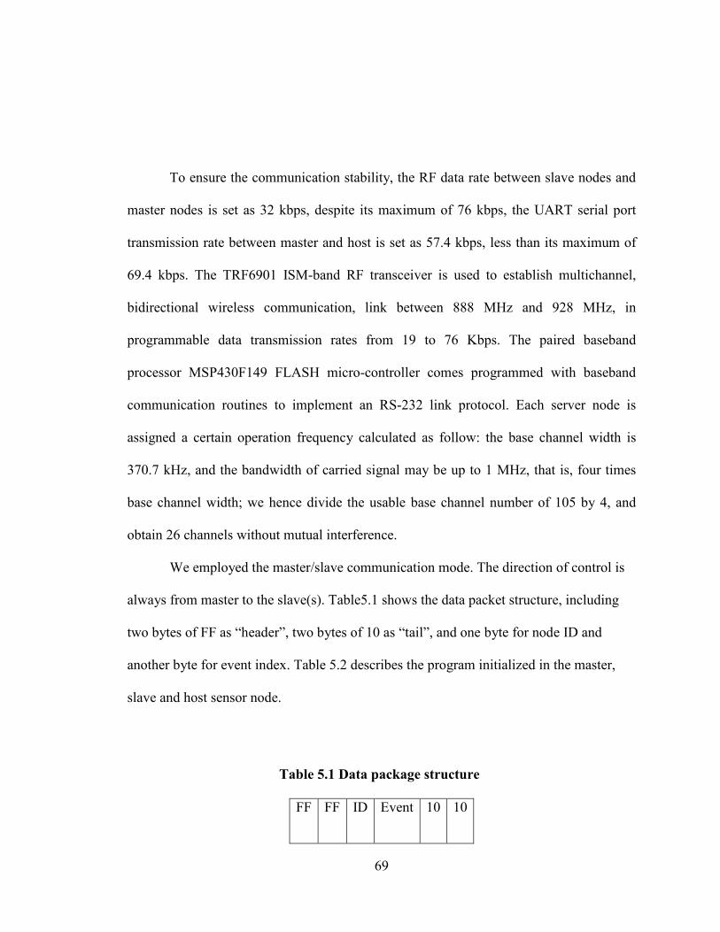
69
To ensure the communication stability, the RF data rate between slave nodes and
master nodes is set as 32 kbps, despite its maximum of 76 kbps, the UART serial port
transmission rate between master and host is set as 57.4 kbps, less than its maximum of
69.4 kbps. The TRF6901 ISM-band RF transceiver is used to establish multichannel,
bidirectional wireless communication, link between 888 MHz and 928 MHz, in
programmable data transmission rates from 19 to 76 Kbps. The paired baseband
processor MSP430F149 FLASH micro-controller comes programmed with baseband
communication routines to implement an RS-232 link protocol. Each server node is
assigned a certain operation frequency calculated as follow: the base channel width is
370.7 kHz, and the bandwidth of carried signal may be up to 1 MHz, that is, four times
base channel width; we hence divide the usable base channel number of 105 by 4, and
obtain 26 channels without mutual interference.
We employed the master/slave communication mode. The direction of control is
always from master to the slave(s). Table5.1 shows the data packet structure, including
two bytes of FF as “header”, two bytes of 10 as “tail”, and one byte for node ID and
another byte for event index. Table 5.2 describes the program initialized in the master,
slave and host sensor node.
Table 5.1 Data package structure
FF FF ID Event 10 10

70
Table 5.2 Communication interface
Slave Node
Initialization RF(size of packet, sub bandwidth assigned, baud rate) while(1) Sampling and Processing() Send RF(sub bandwidth assigned, &packet, size of packet) end
Master Node
Synchronization RF(size of packet, all bandwidth assigned, baud rate) while(1) for i=1:number of sub bandwidth broadcasting Receive RF (sub bandwidth(i), &packet, size of packet) Error Rejection Event Smoothing() Send Serial(node ID, &packet, size of packet, baud rate) end end
Host
Initialization Serial(com#, size of buffer, baud rate) while(1) Find Packet Header() Read Data() Data Fusion Target Tracking() end
71
CHAPTER 6
EXPERIMENTAL WORK
6.1 Introduction
This chapter describes the experiment setup and experimental results. Both path
dependent and path independent recognition results obtained by using the compressive
human recognition scheme introduced in chapter2 and chapter 3 are given. The
distributed tracking results are also given.
6.2 System setup
For path dependent human subject recognition, we used 3 two-column sensor
nodes, as shown in Figure 1.1. The sensor node deployment is shown in Figure 1.2. The
human subjects randomly walk inside a 4m × 4m room one at a time. Each subject
generated one set of data, first half of which would be used for feature model training
while the other half for real time testing. The same setting is also used for path
independent. Regardless whether it is path dependent or path independent, close-set
walker recognition and open-set walker recognition are performed. For close-set
recognition, the system performance is evaluated using identification rate. For open-set
walker recognition, the performance can be plotted in a Receiver Operator Characteristic
(ROC) plot, usually is known as ROC curve.

72
For distributed human subject tracking, 4 tracking sensor nodes shown in Figure
1.3 are used. They are arranged in each of the 4 sides of a 4m × 4m room as shown in
Figure 1.4.
6.3 Path dependent recognition results
For single human subject fixed path recognition, the human subjects walk along a
prescribed path back and forth inside a 4m × 4m room one at a time. By using the
selection method proposed in the previous chapter 2 and chapter 3, 1 bit data is selected
from each of the sensor node, thus the total 3 bits data would be used for building model.
In order to compare the fusion effect, the fusion results are also shown in the same
figures. The close-set identification rate and open-set ROC curve results for 5 targets is
shown below. The results are based on 200 tests of 5 different targets.
Here are some notations that need to be explained first in order to understand the
result plots. In the plot below, S stands for Similarity; SD stands for Similarity Distance;
TS stands for State Transition Similarity; TSD stands for State Transition Similarity
Distance; KL stands for KL Distance; TKL stands for State Transition KL Distance; Set 1
indicate the results is based on the first preselected 3 channels – channel 5, 10 and 22,
one from each node; Set 2 stands for another set of preselected 3 channels – channel 2 10
19. Both sets are selected through the data evaluation methods introduced in 3.4.

73
From the figure below, we can see that when using score fusion scheme with the
KL distance feature to capture the state transition distribution feature of targets, 100
percent identification rate is achieved. It is not hard to see that when set 1 and set 2 can
individually achieve a good performance, the score fusion and help improve the
performance. It can also be seen that the state transition data contains more useful
information than the state data, since the recognition rate is higher for both similarity
distance and KL divergence when using transition data. The open-set ROC curve shown
below also shows the similar results.
Fig 6.1: Close set recognition rate for path dependent recognition using 2 preselected channels, data fusion, feature fusion and score
fusion.

74
Fig 6.2: Open set ROC curve for path dependent recognition using set 1 preselected channels using different features

75
Fig 6.3: Open set ROC curve for path dependent recognition using set 2 preselected channels using different features

76
Fig 6.4: Open set ROC curve for path dependent recognition using score fusion preselected channels using different features

77
6.4 Path independent recognition results
The challenge for path independent recognition is that the random path walk can
generate less regular sequence pattern when compared with fixed path walk, makes it
hard to extract the feature or find the pattern with respect to each individual. Using the
similar process as fixed path could be a solution. That is, we collect the random walk
sample of each human target and use the random walk sequence data to extract the
feature as well as test.
However, in an effort to develop a more general scheme for path independent
recognition, the approach we developed here is to use 2 fixed path patterns as a base, the
random walk sequence feature will be mapped into these two bases and the distances to
both of them are considered for the decision. The main idea behind this is that we believe
no matter which direction the walker walks towards, the 3 sensor nodes should be able to
pick up part of the information that is similar to those contained in the pre-designed fix
path, the diagonal lines in this case. Human brain has the similar function, as one usually
does not need a particular point of view to recognize a person he/she knows is walking.
In computer vision recognition schemes, the same idea is used by finding the static
feature in different images of the same target.
Table 6.1 shows us the recognition rate of 5 targets in 100 tests. Figures below
show us the ROC curve of 200 tests using the idea described above. To compare the

78
recognition results using the traditional random training scheme, the recognition rate
under this scheme is also plotted.
Fig 6.5: Open set ROC curve for path independent recognition using set 1 preselected channels using different features

79
Fig 6.6: Open set ROC curve for path independent recognition using set 2 preselected channels using different features

80
Fig 6.7: Open set ROC curve for path independent recognition with score fusion using different features

81
Table 6.1 Path independent recognition rate using 2 paths based mapping scheme
Sean Alina Nanda Robin Yuan
Sean 83% 1% 4% 12%
Alina 3% 67% 24% 6%
Nanda 2% 21% 71% 6%
Robin 78% 22%
Yuan 2% 3% 11% 84%
Fig 6.8: Close set recognition rate for path independent recognition using random training scheme with 2 preselected channels, data
fusion, feature fusion and score fusion.

82
6.5 Tracking results
4 tracking sensor nodes shown in Figure 1.3 are used. They are arranged in each
of the 4 sides of a 4m × 4m room as shown in Figure 1.4. The figures shown below show
the distributed tracking results capture during a cycle of a single human target walking in
circles clockwise around the room. The black mark in the figures indicate the tracking
target result and the small marks show us the sensor detection beam and detection area
according the sensor response.
Fig 6.9: Snapshot of tracking one human target walking in a circle
in a room. (Frame 15)

83
Fig 6.10: Snapshot of tracking one human target walking in a circle in a room. (Frame 23)
Fig 6.11: Snapshot of tracking one human target walking in a circle in a room. (Frame 36)

84
Fig 6.12: Snapshot of tracking one human target walking in a circle in a room. (Frame 42)
Fig 6.13: Snapshot of tracking one human target walking in a circle in a room. (Frame 50)
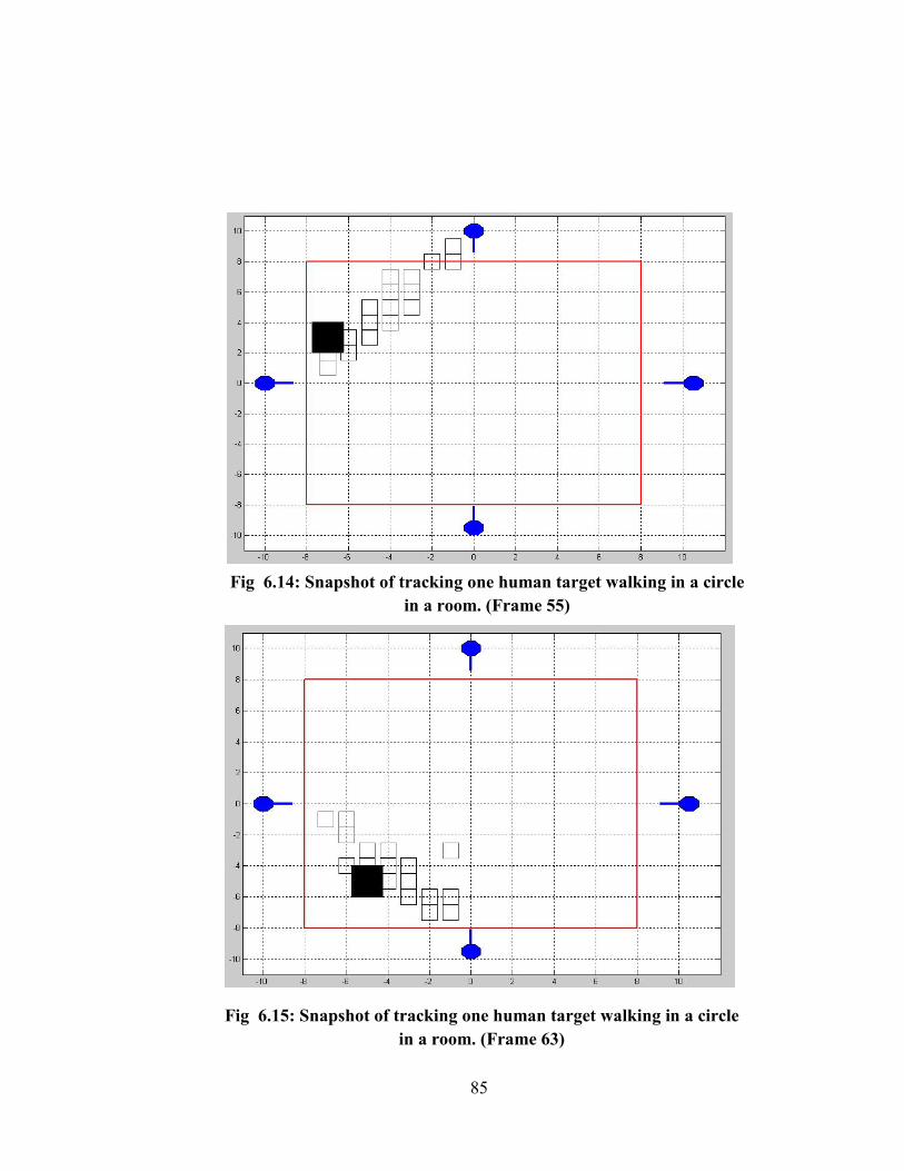
85
Fig 6.14: Snapshot of tracking one human target walking in a circle in a room. (Frame 55)
Fig 6.15: Snapshot of tracking one human target walking in a circle in a room. (Frame 63)

86
Fig 6.16: Snapshot of tracking one human target walking in a circle in a room. (Frame 68)

87
CHAPTER 7
CONCLUSION AND FUTURE SCOPE
With the increasing use of biometric and sensor network and their increasing
impact on the industrial application, it is important to understand the disciplines in this
area. Adopting tools used in these different disciplines, methods of inquiry can be
formulated that allow for the interpretation of works that are both technically sound and
sociologically insightful.
This thesis presented a compressive gait biometrics. Based on previous work, we
developed an integrated sensing and processing framework for compressive gait
biometrics. Gait biometrics is advantageous in their capability of recognition at a distance
under changing environmental and cosmetic conditions. Gait-based human recognition
tolerates low resolution of sensory data and allows for non-cooperative subjects under
examination. The central issue of our research is the selection of representative features
that describe the specific way one carries the body or makes gestures, idiosyncratic
rhythms of arm swing, leg crossing or utterance, and possibility distribution of habitual
trajectories. To conquer this problem, we developed a scheme includes data evaluation,
feature extraction and feature fusion, which enable us to achieve a high recognition rate
of the system.
The main contributions for our work are:

88
1. We proposed a distributed compressive sampling structure for gait information
acquisition includes multiplex field of view modulation of sensors and object
space segmentation with distributed sensor deployment. The former refers to the
use of coded masks (obscurants) that allows or blocks one sensor to detect
motions with several regions in the object space, the latter refers to the
deployment of sensor that segments the object space into many cells, each
characterized by its Boolean visibility to sensors.
2. We developed an incoherent sensing protocol for gait feature extraction, which
allow us to further reduce the redundant sensory data amount and extract feature
data in concise forms. This is achieved by multichannel sampling and switching,
as well as sparse gait feature representation in terms of logic parameters of
probability distributions of signal states and their transitions. The central task of
compressive sensing protocol development is to choose a proper scheme of the
random projection encoding and linear program decoding. It involves two steps:
finding a set of proper temporal spatial bases and choosing a set of measurement
functions accordingly. In our study, we studied the non-adaptive random
measurement functions, in both spatial and temporal domains for preprocessed
sequence data. Through compressive sensing protocols, the gait attributes will be
transformed into compressed sensory signals. Sensory data feature will be further
extracted from those compressed signals as far as the spatial/ temporal coherence
and statistical properties are preserved.

89
3. We investigated several decentralized information aggregation schemes for
distributed sensors. With the help of information aggregation among sensor
groups, which can happen at data, feature, score and decision levels, we further
improve the performance of the recognition system. Data level fusion accepts
high quality samples and rejects poor quality ones. Feature level fusion relies on
building inclusive feature models. Score level fusion combines distributed scores.
Decision level fusion combines decisions from different processing units by logic
rules. Given the prior knowledge about the sensor head information and the
physical space resource allocation, compressive sensors convert the raw
information into a feature field, which can be reduced by low-level processing
and transformed through fusion into a feature pattern representation. Finally, the
logic parameters of feature patterns are statistically analyzed for computing
similarity and making recognition decisions.
4. We implemented a distributed tracking scheme in real system. From the achieved
experimental results, we believe that the pyroelectric sensor will rise to one
mainstream human detection instrument, besides its video and audio counterparts,
and offer one more dimension for all the applications of human-machine
interfaces. It can not only run as a stand-alone inmate/patient monitoring system
under all illumination conditions, but also serve as a complement for conventional
video and audio human tracking systems.

90
Several interesting questions appeared during this research are still remain to be
unsolved. These questions are likely to be our future work.
(1) The most important one among them is what limitation in clothing, physical,
medical and emotional biometrics is on the gait biometric in our system? The
following figure shows the sensor data and the data state transition of the
same target under different speed conditions and different clothing conditions.
The feature we currently used in our system is not stable for this problem, thus
will lead the system to a failure recognition decision result.
Fig 7.1: Sensory data for same human target under
different speed conditions
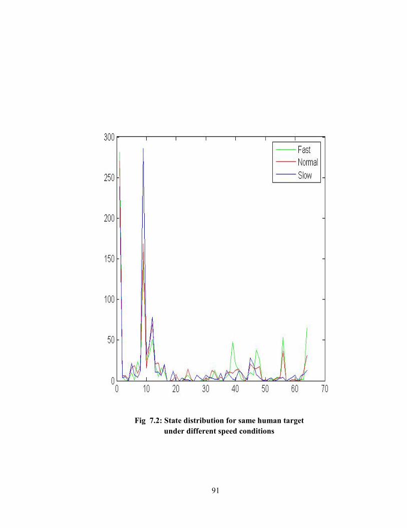
91
Fig 7.2: State distribution for same human target
under different speed conditions

92
Fig 7.3: Sensory data for same human target under different cloth conditions
Fig 7.4: State transition for same human target under different cloth conditions

93
(2) What is the optimal field of view mask design for our system? Different
visibility layouts will create pyroelectric sensor systems with different
capabilities: one good for motion detection, another for feature extraction. To
the human identification, two types of visibility modulation can be further
tested, namely the periodic and the random. In capturing motions of the
human body along the vertical direction, a periodic visibility modulation of a
sensor array functions as spatial filters with a specific passing band. A
(pseudo-)random visibility modulation of a sensor array yields a set of spatial
filters with orthogonal passing bands. The study of these two types visibility
modulation would improve human identification rates.
(3) What is the optimal random multi-channel sampling scheme in both spatial
and temporal domain for gait attributed acquisition?
(4) What are the proper sparse representations of shape and dynamic features of
gait biometrics in our system?
(5) The distributed tracking algorithm discussed here is only based the predefined
setting including sensor nodes position and so on. How to generate a self
calibration scheme to automatically calculate the position is also a very
challenging problem.
The scope of future work will also include advanced Integration of Tracking and
Identification. A fully functional real-time multiple human tracking and identification
system demands the ability to discriminate the sensory data source, it will also require

94
short testing event sequences for fast walker identification and multiple object
recognition at the same time.

95
REFERENCES
1) M.M. Trivedi, K.S. Huang and I. Mikic, “Dynamic context capture and distributed video arrays intelligent spaces,” IEEE Trans. Syst., Man, Cybern. A, vol. 35, no. 1, pp. 145-163, Jan. 2005
2) T. Zhao and R. Nevatia, “Tracking multiple humans in complex situations," IEEE Trans. Pattern Anal.Machine Intell., vol. 26, no. 9, pp. 1208-1221, Sept. 2004.
3) D. Comaniciu, V. Ramesh, and P. Meer, “Kernel-based object tracking," IEEE Trans.
Pattern Anal. Ma-chine Intell., vol. 25, no. 5, pp. 564-577, May 2003.
4) Y. Ricquebourg and P. Bouthemy, “Real-time tracking of moving persons by exploiting spatio-temporal image slices," IEEE Trans. Pattern Anal. Machine Intell., vol. 22, no. 8, pp. 797-808, Aug. 2000.
5) W. Hu, T. Tan, L.Wang, and S. Maybank, “A survey on visual surveillance of object
motion and behaviors,"IEEE Trans. Syst., Man, Cybern. C, vol. 34, no. 3, pp. 334-352, Aug. 2004.
6) B. Lin and R. Chellappa, “A generic approach to simultaneous tracking and
veri¯cation in video," IEEE Trans. Image Processing, vol. 11, no. 5, pp. 530-544, May 2002.
7) D. Li, K. D. Wong, Y. H. Hu, and A. M. Sayeed, “Detection, classification, and
tracking of targets," IEEE Signal Processing Mag., vol. 19, no. 2, pp. 17-29, Mar. 2002.
8) J. Vermaak, S. Maskell, and M. Briers, “Tracking a variable number of targets using
the existence joint probabilistic data association fillter," IEEE Trans. Signal Processing, vol. 33, no. 1, pp. 752-769, Jan. 2005.
9) C. Stiller and J. Konrad, “Estimating motion in image sequences," IEEE Signal
Processing Mag., vol. 16,no. 4, pp. 70-91, July 1999.
10) R. H. Anderson and J. L. Krolik, “Track association for over-the-horizon radar with a statistical ionospheric model," IEEE Trans. Signal Processing, vol. 50, no. 11, pp. 2632-2643, Nov. 2002.

96
11) S. S. Blackman, “Multiple hypothesis tracking for multiple target tracking," IEEE
Aerosp. Electron. Syst. Mag, vol. 19, no. 1, pp. 5-18, Jan. 2004.
12) T. E. Fortmann, Y. Bar-Shalom, and M. Scheffe, “Sonar tracking of multiple targets using joint probabilistic data association," IEEE J. Oceanic Eng., vol. 8, no. 3, pp. 173-184, July 1983.
13) K.-C. Chang, C.-Y. Chong, and Y. Bar-Shalom, “Joint probabilistic data association
in distributed sensor networks," IEEE Trans. Automat. Contr., vol. 31, no. 10, pp. 889-897, Oct. 1986.
14) C. Hue, J.-P. L. Cadre, and P. Perez, “Sequential monte carlo methods for multiple
target tracking and data fusion," IEEE Trans. Signal Processing, vol. 50, no. 2, pp. 309-325, Feb. 2002.
15) T. Vercauteren, D. Guo, and X. Wang, “Joint multiple target tracking and
classification in collaborative sensor networks," IEEE J. Select. Areas Commun., vol. 23, no. 4, pp. 714-723, Apr. 2005.
16) M. Orton and W. Fitzgerald, “A Bayesian approach to tracking multiple targets using
sensor arrays and particle filters," IEEE Trans. Signal Processing, vol. 50, no. 2, pp. 216-223, Feb. 2002.
17) C.-Y. Chong and S. P. Kumar, “Sensor networks: evolution, opportunities, and
challenges," Proc. IEEE, vol. 91, no. 8, pp. 1247-1256, Aug. 2003.
18) J. C. Chen, K. Yao, and R. E. Hudson, “Source localization and beamforming," IEEE Signal Processing Mag., vol. 19, no. 2, pp. 30-39, Mar. 2002.
19) F. Zhao, J. Shin, and J. Reich, “Information-driven dynamic sensor collaboration,"
IEEE Signal Processing Mag., vol. 19, no. 2, pp. 61-72, Mar. 2002.
20) S. B. Lang, “Pyroelectricity: from ancient curiosity to modern imaging tool," Physics Today, vol. 58, no. 8, pp. 31-35, Aug. 2005.
21) S. J. Kang, V. B. Samoilov, and Y. S. Yoon, “Low-frequency response of pyroelectric
sensors," IEEE Trans. Ultrason., Ferroelect., Freq. Contr., vol. 45, no. 5, pp. 1255-1260, Sept. 1998.

97
22) A. Hossain and M. H. Rashid, “Pyroelectric detectors and their applications," IEEE Trans. Ind. Applicat.,vol. 27, no. 5, pp. 824-829, Sept. 1991.
23) A. Sixsmith, N. Johnson, and R. Whatmore, “Pyroelectric ir sensor array for fall
detection in the older population," J. Phys. IV France, vol. 128, pp. 153-160, 2005.
24) A. S. Sekmen, M. Wilkes, and K. Kawamura, “An application of passive human-robot interaction: human tracking based on attention distraction," IEEE Trans. Syst., Man, Cybern. A, vol. 32, no. 2, pp. 248-259, Mar. 2002.
25) J. Wayman, A. Jain, D. Maltoni, and D. Maio, Biometric Systems. Reading, London,
UK: Springer, 2005.
26) P. J. Phillips, A. Martin, C. L. Wilson, and M. Przybocki, “An introduction to evaluating biometric systems," IEEE Computer, vol. 33, no. 2, pp. 56{63, Feb. 2000.
27) J. Han and B. Bhanu, “Individual recognition using gait energy image," IEEE Trans.
Pattern Anal. Machine Intell., vol. 28, no. 2, pp. 316{322, Feb. 2006.
28) N. V. Boulgouris, D. Hatzinakos, and K. N. Plataniotis, “Gait recognition," IEEE Signal Processing Mag., vol. 22, no. 6, pp. 78{90, Nov. 2005.
29) U. Gopinathan, D. J. Brady, and N. P. Pitianis, “Coded aperture for efficient
pyroelectric motion tracking," Opt. Exp., vol. 11, no. 18, pp. 2142{2152, Nov. 2003.
30) M. Shankar, J. Burchett, Q. Hao, B. D. Guenther, and D. J. Brady, “Human-tracking systems using pyro-electric detectors," Opt. Engr., vol. 45, no. 10, pp. 106 401(1{10), Oct. 2006.
31) T. M. Hussain, A. M. Baig, T. N. Saddawi, and S. A. Ahmed, “Infrared pyroelectric
sensor for detection of vehicular traffic using digital signal processing techniques," IEEE Trans. Veh. Technol., vol. 44, no. 3, pp. 683{689, Aug. 1995.
32) S. B. Lang, “Pyroelectricity: from ancient curiosity to modern imaging tool," Physics
Today, vol. 58, no. 8, pp. 31{35, Aug. 2005.
33) M. S. Nixon, T. Tan, and R. Chellappa, Human identification based on gait. Reading, NY: Springer, 2006.

98
34) J. B. Hayfron-Acquah, M. S. Nixon, and J. N. Carter, “Automatic gait recognition by symmetry analysis," Pattern Recognition Letters, no. 24, pp. 2175{2183, 2003.
35) L. Havasi, Z. Szlavik, and T. Sziranyi, “Higher order symmetry for non-linear
classification of human walk detection," Pattern Recognition Letters, no. 27, pp. 822{829, 2006.
36) R. J. Mammone, X. Zhang, and R. P. Ramachandran, “Robust speaker recognition: a
feature-based approach," IEEE Signal Processing Mag., vol. 13, no. 5, pp. 58{71, Sept. 1996.
37) L. R. Rabiner, “A tutorial on hidden markov models and selected applications in
speech recognition," Proc. IEEE, vol. 77, no. 2, pp. 257{286, Feb. 1989.
38) H. Pan, S. E. Levinson, T. S. Huang, and Z.-P. Liang, “A fused hidden Markov model with application to bimodal speech processing," IEEE Trans. Signal Processing, vol. 52, no. 3, pp. 573{581, Mar. 2004.
39) M. Faundez-Zanuy and E. Monte-Moreno, “State-of-the-art in speaker recognition,"
IEEE Aerosp. Electron. Syst. Mag, vol. 20, no. 5, pp. 7{12, May 2005.
40) D. J. Brady, N. P. Pitsianis, and X. Sun, “Reference structure tomography," J. Opt. Soc. Am. A, vol. 21, no. 7, pp. 16{18, July 2004.
41) R. G. Baraniuk, “Compressive sensing," IEEE Signal Processing Mag., vol. 24, no. 4,
pp. 118{124, July 2007.
42) M. J. Beal, “Variational algorithms for approximate Bayesian inference," Ph.D. dissertation, Univ. of London, May 2003.
43) M. Harwit and N. J. A. Soane, Hadamard Transform Optics. Reading, NY: Academic
Press, 1979.
44) A. Busboom, H. D. Schotten, and H. Elders-Boll, “Coded aperture imaging with multiple measurements," J. Opt. Soc. Am. A, vol. 14, no. 5, pp. 1058{1065, May 1997.
45) A. K. Jain, A. Ross, and S. Prabhakar, “An introduction to biometric recognition,"
IEEE Trans. Circuits Syst. Video Technol., vol. 14, no. 1, pp. 4{20, Jan. 2004.

99
46) Qi Hao, "Multiple human tracking and identification with wireless distributed pyroelectric sensors," PhD Thesis, Duke University, May, 2006.
47) Mohan Shankar, John Burchett, Qi Hao, etc., "Characterization of pyroelectric
infrared detectors for human tracking," Optical Engineering, no. 45, vol. 10, pp. 106401(1-10), Dec. 2006.
48) Qi Hao, Jian-Shuen Fang, David J. Brady, Bob D. Guenther, and Mohan Shankar,
"Human tracking with wireless distributed pyroelectric sensors," IEEE Sensors Journal, vol. 6, no. 6, pp. 1683-1694, Dec. 2006.
49) Qi Hao, Jian-Shuen Fang, David J. Brady, and Bob D. Guenther, "Real-time walker
recognition using pyroelectric sensors," IEEE Sensors Journal, submitted, 2006. 50) Qi Hao, Jian-Shuen Fang, David J. Brady, Bob D. Guenther, and Mohan Shankar,
"Tracking and identifying multiple humans with wireless geometric pyroelectric sensors," IEEE Sensors Journal, submitted, 2006.
51) Li, N. and Hao, Qi, "Multiple human tracking with wireless distributed pyroelectric
sensors,'' Proc. of SPIE Defense and Security, March 2008, pp. 694033(1-12). 52) Li, N. and Hao, Qi, "Multiple walker recognition with wireless distributed
pyroelectric sensors,'' Proc. of SPIE Defense and Security, March 2008, pp. 694034(1-12).
53) Donal McErlean, Shrikanth Narayanan, “Distributed detection detection and tracking
in sensor networks”, 36th Asilomar Conference on Signal, system and computers, 2002 54) R.R. Brooks, P. Ramanathan and A.M. Sayeed, “Distributed target classification and
tracking in sensor networks”, Spcial issue on sensor networks, January 2003.


![Biometric User Authentication on Smartphone …csis.pace.edu/~ctappert/it691-projects/techreports/2014...accelerometer-based biometric analysis for gait recognition [2][10][14][22].](https://static.fdocuments.in/doc/165x107/5f4d0f2f6cdd9c7fd650e094/biometric-user-authentication-on-smartphone-csispaceeductappertit691-projectstechreports2014.jpg)


![Face and Voice Fusion for Human Recognition in Non-controlled … · 2018-08-29 · biometric recognition including fingerprints, face, voice, iris, hand and gait [3]. Every biometric](https://static.fdocuments.in/doc/165x107/5f42211f0300b86f963dac1e/face-and-voice-fusion-for-human-recognition-in-non-controlled-2018-08-29-biometric.jpg)
