Comprehensive Meta Analysis Version 2.0

This manual will continue to be revised to reflect changes in the program. It will also be expanded to include chapters covering conceptual topics. Upgrades to the program and manual will be available on our download site.

1

Comprehensive Meta Analysis Version 2 Developed by Michael Borenstein Larry Hedges Julian Higgins Hannah Rothstein Advisory group Doug Altman Betsy Becker Jesse Berlin Harris Cooper Despina Contopoulos-Ioannidis Kay Dickersin Sue Duval Matthias Egger Kim Goodwin Wayne Greenwood Julian Higgins John Ioannidis Spyros Konstantopoulos Mark Lipsey Michael McDaniel Fred Oswald Terri Pigott Stephen Senn Will Shadish Jonathan Sterne Alex Sutton Steven Tarlow Thomas Trikalinos Jeff Valentine John Vevea Vish Viswesvaran David Wilson This project was funded by the National Institutes of Health

2

Group meetings to develop the program

July 2002. Left to right (Seated) Vish Viswesvaran, Will Shadish, Hannah Rothstein, Michael Borenstein, Fred Oswald, Terri Pigott. (Standing) Spyros Konstantopoulos, David Wilson, Alex Sutton, Jonathan Sterne, Harris Cooper, Sue Duval, Jesse Berlin, Larry Hedges, Mike McDaniel, Jack Vevea

August, 2003. Left to right (Seated) David Wilson, Betsy Becker, Julian Higgins, Will Shadish, Hannah Rothstein, Michael Borenstein, Mike McDaniel, Steven Tarlow. (Standing) Spyros

Konstantopoulos, Larry Hedges, Harris Cooper, John Ioannidis, Despina Contopoulos-Ioannidis, Jack Vevea, Sue Duval, Mark Lipsey, Alex Sutton, Terri Pigott, Fred Oswald, Wayne Greenwood,

Thomas Trikalinos.

3

August, 2004 Left to right: Jonathan Sterne, Doug Altman, Alex Sutton, Michael Borenstein, Julian Higgins, Hannah Rothstein

4

Introduction The program installation will create a shortcut labeled Comprehensive Meta Analysis V2 on your desktop and also under “All programs” on the Windows Start menu. It will also install several data files for use with this guide. These files will be installed in “Demo Files”, beneath the program directory, which (by default) will be C:\Program Files\Comprehensive Meta Analysis Version 2. Within “Demo Files”, select files from the language directory appropriate for your computer’s language settings. To uninstall the program use the Windows Control panel, select “Add or Remove Programs”, and remove “Comprehensive Meta Analysis Version 2”

This document includes the following sections.

Introduction .....................................................................................................................5 Section 1. Basic data entry and analysis.....................................................................7

The tutorial.....................................................................................................................8 Create columns for effect size data .............................................................................10 Effect size wizard.........................................................................................................11 Modify data entry column names.................................................................................14 Enter effect size data...................................................................................................15 View computational formulas.......................................................................................16 Diagnose data entry problems.....................................................................................17 Bookmark entered data ...............................................................................................18 Customize effect size index display.............................................................................19 Launch analysis module ..............................................................................................21 View summary statistics ..............................................................................................24 View study weights ......................................................................................................25 View standardized residuals........................................................................................26 View ‘One study removed’ results ...............................................................................27 View cumulative analysis.............................................................................................28 View calculations .........................................................................................................29 Filter the analysis …....................................................................................................30 Some tools for customizing the analysis display .........................................................31

Section 2. Multiple data entry formats ........................................................................33 Overview......................................................................................................................34 Step-by-step instructions for multiple formats .............................................................35 Create the second effect size entry block....................................................................36 Select second effect size entry format.........................................................................37 Enter data for second effect size .................................................................................38 View analysis...............................................................................................................39

Section 3. Working with moderator variables ............................................................40 Create the moderator column......................................................................................41 Enter moderator values ...............................................................................................42 Select a grouping variable ...........................................................................................43 Run Group by… analysis.............................................................................................44 Select a computational model .....................................................................................45

5

View additional statistics by group...............................................................................46 Recode column values ................................................................................................47

Section 4. Subgroups within studies ..........................................................................49 Create column for subgroups within study ..................................................................50 View analysis...............................................................................................................51 Use study as the unit of analysis .................................................................................52 Multiple sets of subgroups...........................................................................................53 Filter subgroup sets for analysis..................................................................................54

Section 5. Multiple outcomes within studies.............................................................55 Create the outcome column ........................................................................................56 Enter outcome values..................................................................................................57 View analysis for one outcome....................................................................................58

Section 6. Importing data from other programs........................................................59 Import data from Excel ................................................................................................60 Paste data into the data entry module.........................................................................61 Assign column header titles.........................................................................................62 Assign a ‘Study name’ column ....................................................................................63 Identify the effect size columns ...................................................................................64 Select effect size entry format .....................................................................................65 Assign effect size entry columns .................................................................................66 Import data with multiple outcomes per row ................................................................68 Import data with multiple effect size entry formats ......................................................71

Section 7. Saving and loading files ............................................................................72 Save the data set.........................................................................................................73 Open and load the saved data set...............................................................................74

Section 8. Publication-quality graphics .....................................................................75 Modify analysis display................................................................................................76 Launch graphics module .............................................................................................77 Format graphics display ..............................................................................................78 Change computational model......................................................................................79 Select color scheme for presentation format ...............................................................81 Format text ..................................................................................................................82 Export to file.................................................................................................................83

Section 9. Meta regression..........................................................................................84 Define a moderator......................................................................................................85 Launch the Meta regression module ...........................................................................86 Select the moderator ...................................................................................................87 View the regression scatter plot .................................................................................88 Adjust scatter plot display............................................................................................89 Select the regression model ........................................................................................90 View iterations .............................................................................................................91 View data and residuals ..............................................................................................92

Section 10. Publication Bias .......................................................................................93 Funnel plot...................................................................................................................94 Duval and Tweedie’s trim and fill.................................................................................96 Begg and Mazumdar rank correlation .........................................................................98 Egger’s regression intercept........................................................................................99 Fail-safe N .................................................................................................................100

Section 11. Data Entry Templates ............................................................................101 View templates ..........................................................................................................102 Select a template.......................................................................................................103

6

Section 1. Basic data entry and analysis This section shows how to set up a spreadsheet for data entry and run the basic analyses.

7

The tutorial

The program includes a tutorial which may be opened from the Help menu. The tutorial covers the same material that is explained on the following pages.

8

Overview The program uses a spreadsheet for data entry, but requires the user to identify specific columns to hold the study names and the effect size data. This process is explained here.

Create a column for Study Names Select Insert… Column for… Study names.

The program will insert a column for study names as shown below.

Select Insert… Column for… Study names.

The program inserts this column.

9

Create columns for effect size data Select Insert… Column for… Effect size data.

Select Insert… Column for… Effect size data.

This will launch a wizard that allows the user to select the desired format (or formats).

10

Effect size wizard (Screen 1)

The first screen in the wizard (above) offers an overview of the options for entering effect size data, as follows:

“If you have already computed the effect size (such as the standardized mean difference or the log odds ratio) for each study, you may enter this information directly.

“Or, you may provide summary data (such as the number of events or the means and standard deviations), and the program will compute the effect size automatically.

“Use this wizard to specify the type of data you plan to enter, and the program will create the required columns.

“The program allows you to enter effect size data in more than one format. You will create one set of effect size columns now, and may add additional sets at any time.

11

Effect size wizard (Screen 2)

The second screen of the wizard is shown here, and allows the user to select the class of data entry types:

• Comparison of two groups, interventions, or exposures (includes correlations) • Estimate of means, proportions, or rates in one group at one time-point • Generic point estimates • Generic point estimates, log scale For the running example of the BCG data, select the first option.

12

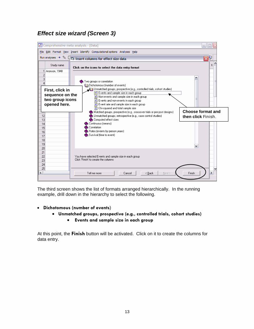
Effect size wizard (Screen 3)

First, click in sequence on the two group icons opened here.

Choose format and then click Finish.

The third screen shows the list of formats arranged hierarchically. In the running example, drill down in the hierarchy to select the following.

• Dichotomous (number of events)

• Unmatched groups, prospective (e.g., controlled trials, cohort studies) • Events and sample size in each group

At this point, the Finish button will be activated. Click on it to create the columns for data entry.

13

Modify data entry column names

If desired, modify the default names for data entry columns.

The wizard will close and the program will automatically offer this dialog for modifying effect size format column names. If, for example, you elect to substitute “Treated” for “Group-A” and “Control” for “Group-B”, you will create column names such as “Treated events” and “Control events”.

The modifications made here will be applied not only to the format selected, but also to columns in any related format (in this case, in formats of the “cohort or prospective studies” type). The dialog gives name override suggestions consistent with the format type but will accept any user-entered value.

14

Enter effect size data

Enter data here. Program computes effect size and displays it here.

When the group names dialog closes, the spreadsheet looks like this. White columns are used for entering data. Yellow columns display the computed effect size. Note that the entry column names have been modified (“Treated” and “Control” in place of the defaults, “Group-A” and “Group-B”).

In the white columns enter the “Number of Events” and “Total N” for the treated group (4, 123) and the control group (11, 139).

The program automatically computes the odds ratio (0.391) as well as the log odds ratio and its standard error (-.939, .598) and displays these in the yellow columns.

15

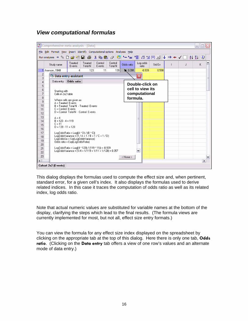
View computational formulas

Double-click on cell to view its computational formula.

This dialog displays the formulas used to compute the effect size and, when pertinent, standard error, for a given cell’s index. It also displays the formulas used to derive related indices. In this case it traces the computation of odds ratio as well as its related index, log odds ratio.

Note that actual numeric values are substituted for variable names at the bottom of the display, clarifying the steps which lead to the final results. (The formula views are currently implemented for most, but not all, effect size entry formats.)

You can view the formula for any effect size index displayed on the spreadsheet by clicking on the appropriate tab at the top of this dialog. Here there is only one tab, Odds ratio. (Clicking on the Data entry tab offers a view of one row’s values and an alternate mode of data entry.)

16

Diagnose data entry problems

When the data are not valid, the effect size results can’t be computed. To diagnose the problem, simply move the mouse over any of the cells highlighted in red. The related problem description displays in a pop-up.

17

Bookmark entered data

It is sometimes helpful to bookmark the current data entry state. This step allows you to discard subsequent changes and return to the bookmarked state.

First, click on the Bookmark icon, circled above. In this example, the icon was clicked before entry of the second study.

To restore the bookmarked state, click on Edit… Restore data. After a confirmation prompt, the data are restored, as displayed in the image below.

18

Customize effect size index display

By default the program will display one or two indices (in this case, odds ratio and log odds ratio), which are based on the format selected for data entry. However, the user can customize the screen to display other indices as well.

Right-click on the yellow columns to open the pop-up menu (below). Then click Set primary index or Customize display to launch the index dialog box shown below. (Note that indices in the same color group are compatible with each other. Entry formats associated with indices in one of the color groups can’t be combined in an analysis with formats whose indices belong to another color group).

19

Open data set Before proceeding to the analysis screen, the user would need to enter data for all studies.

As a time-saving device a copy of this data set has been included on the CD. To open this data set select File… Open and then drill down to the location of the data set.

By default, the data set will be in the directory C:\Program Files\Comprehensive Meta Analysis Version 2\Demo Files. The data set name is BCG.

20

Launch analysis module

Click on either button to launch the analysis.

Note: The BCG meta analysis data set is the basis for this and other examples. It will be altered at certain points for the purposes of the presentation.

21

Analysis

Modify the analysis display with these icons.

Set the computation model with these tabs.

Set the analysis display with the bottom tabs.

The primary index from the Data Entry module (in this case odds ratio) is used for the initial Analysis display. The columns labeled Statistics for each study include the odds ratio and 95% confidence interval for each study. The last row in the spreadsheet shows the summary data. Under the fixed effect model the point estimate is 0.647 (0.595, 0.702).

The same information is captured by the Forest plot at the center of the screen. This plot shows each study as a point estimate with its lower and upper limit, and provides a sense of the study-to-study dispersion.

This screen may be customized in many ways, including the following (see toolbar):

• In the Format menu dropdown there are options to:

o Display, hide and modify the appearance of the individual column blocks: Basic stats, Forest plot, Counts, Weights and Residuals.

o Modify the appearance (font, decimal precision etc.) of the screen as a whole. • From the View… Columns menu dropdown, the Moderators option will present a list

of moderators. The user can select from the list and place the selected column where desired in the Analysis display.

• In the Computational options menu dropdown: o The Group by… entry allows the user to run the analysis grouped by a

moderator (if moderators are included in the data set), and to compare the treatment effect across groups.

22

o A drop-down box allows the user to set the Confidence level (95% in this example).

• Right-clicking on a column’s heading area offers a list of context-sensitive entries, including:

o Sort options, both ascending and descending.

o A Customization option which allows the user to modify an individual column’s display (alignment, decimal precision etc.).

o A Scale option (applicable to Forest plot) which allows the user to modify the display scale.

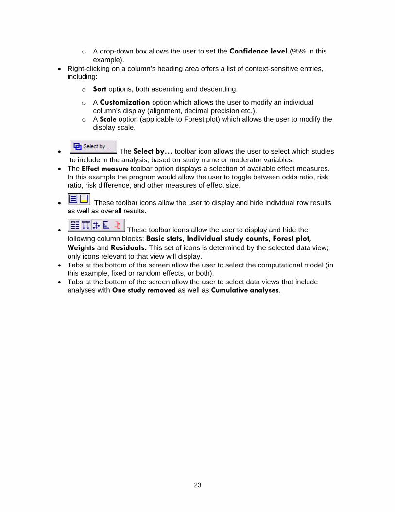
• The Select by… toolbar icon allows the user to select which studies to include in the analysis, based on study name or moderator variables.

• The Effect measure toolbar option displays a selection of available effect measures. In this example the program would allow the user to toggle between odds ratio, risk ratio, risk difference, and other measures of effect size.

• These toolbar icons allow the user to display and hide individual row results as well as overall results.

• These toolbar icons allow the user to display and hide the following column blocks: Basic stats, Individual study counts, Forest plot, Weights and Residuals. This set of icons is determined by the selected data view; only icons relevant to that view will display.

• Tabs at the bottom of the screen allow the user to select the computational model (in this example, fixed or random effects, or both).

• Tabs at the bottom of the screen allow the user to select data views that include analyses with One study removed as well as Cumulative analyses.

23

View summary statistics

Toggle between views.

The Next table button on the toolbar allows you to toggle between two windows, the analysis spreadsheet above and the table below (which provides more detail on the point estimate and heterogeneity).

24

View study weights

• Click on the icon at the top of the screen to display Study weights. (The option is also accessible from the View… Columns menu dropdown.)

• Click on the Both models tab, circled at the bottom of the screen. The spreadsheet now includes two rows at the bottom – labeled Fixed and Random

At the right, the program shows the weight assigned to each study under the fixed or random effects model. Compare, for example, the fixed effect and random effects weights for the “Madras, 1980” study.

In this display, the Z-value and p-value columns and the Events / Total block have been hidden. To hide a block, click on its toggle icon at the top of the screen, or right-click on the block itself and turn off the toggle icon from the resulting dropdown list.

The dropdown list also allows the user to display or hide individual columns within a block. To hide individual columns in the ‘Basic stats’ block, as is done above, right-click on the block and select the ‘Customize display’ option. In the customization dialog, uncheck the column(s) to be hidden.

25

View standardized residuals

Here, the user has clicked on the Residuals icon, circled at the top.

Note, once again, how the display clarifies the contrast in results between the fixed and random models.

26

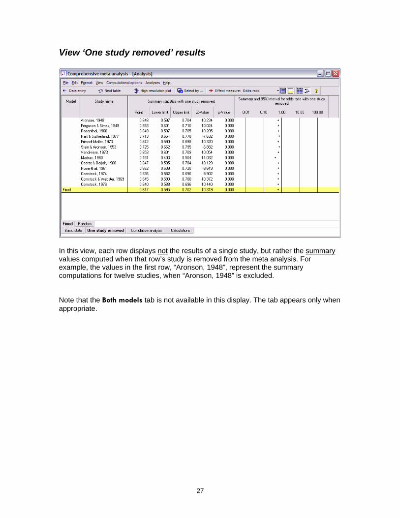
View ‘One study removed’ results

In this view, each row displays not the results of a single study, but rather the summary values computed when that row’s study is removed from the meta analysis. For example, the values in the first row, “Aronson, 1948”, represent the summary computations for twelve studies, when “Aronson, 1948” is excluded.

Note that the Both models tab is not available in this display. The tab appears only when appropriate.

27

View cumulative analysis

The Cumulative analysis option displays results accumulated over successive studies. That is, the second row presents a summary analysis comprising the first two studies (in this case, “Aronson, 1948” and “Ferguson & Simes, 1949”), the third row presents a summary analysis comprising the first three studies, and so on through the final row. When the data are sorted by year, this would show the conclusions that could have been obtained at any point in time with each new study’s appearance.

The Forest plot and the study weight block also display cumulative values.

Note that the studies have been sorted (by year in this case) in order to make the display more meaningful. The image below shows one way such a sort could be done.

In the Data Entry module populate a column with sort values (in this case, year) and click on the circled icon to perform the sort.

28

View calculations

This tab shows how data in each row are summed to yield totals, which are then used to compute the point estimates and standard errors.

This is intended both as a teaching tool and also to allow researchers to understand the precise formula being used. As development continues, the user will be allowed to open a box that shows the precise formula used for each computation, and how these values were inserted into that formula to yield the reported statistics.

29

Select by…

Click on the Select by… icon to launch this dialog. Here you can change the set of studies to include in the meta analysis. If the data set included subgroups or moderator variables, they would appear here as well.

Click on Apply or OK to apply the changes.

30

Some tools for customizing the analysis display

Right-click on the Forest plot block and click on the Scale option to select a different scale setting for the Forest plot. The options for log scales appear when odds ratios, risk ratios, rate ratios, or hazard ratios are used as the effect size index. Otherwise, options for raw scales appear.

Click on the Effect measure option and select a setting in this dropdown to use an alternate measure for the meta analysis computations.

31

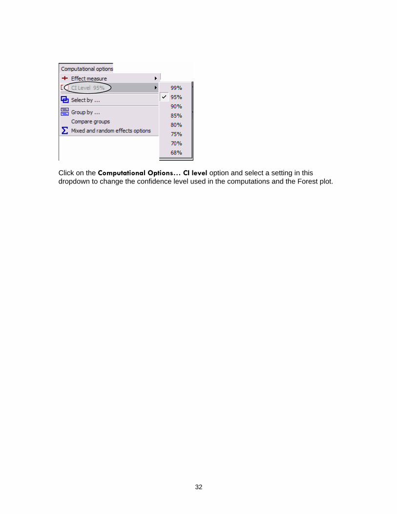
Click on the Computational Options… CI level option and select a setting in this dropdown to change the confidence level used in the computations and the Forest plot.

32

Section 2. Multiple data entry formats If the effect size for all studies is in the same format (e.g., number of events and total N for treated and control groups, or the odds ratio and confidence interval) the user would create one set of columns for effect size data as described in the previous section.

In the event that some studies report the effect size in one format while others report it using another format, the user will need to create two (or more) sets of data entry columns. The options are explained in this section.

This section uses the “Strepokinase” example, which is patterned after a published meta analysis but includes fictional data.

For all studies in this meta analysis, patients who arrive at a hospital following a myocardial infarction are randomized to one of two groups: (A) standard treatment alone, or (B) standard treatment plus streptokinase.

Some studies report the number of events (deaths) and the total number of patients in each group. This data will be used to compute an odds ratio, with odds ratios less than one indicating that patients in the treated group were less likely to die.

Other studies report the odds ratio and the 95% confidence interval.

By default, data sets are copied to C:\Program Files\Comprehensive Meta Analysis Version 2\Demo Files. The two datasets used in this section are StreptoMultiformat18 studies, which includes the 18 studies in the first format, and StreptoMultiformat22 studies, which includes all 22 studies.

33

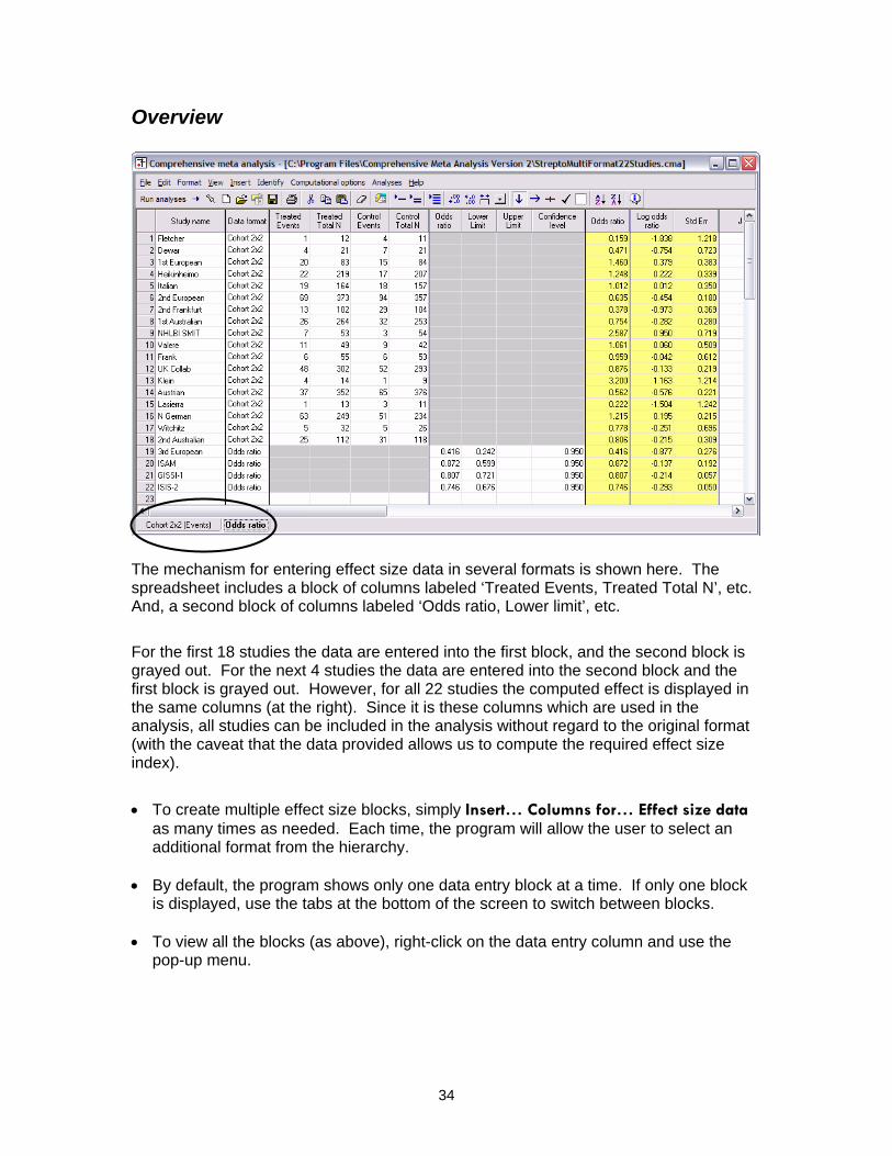
Overview

The mechanism for entering effect size data in several formats is shown here. The spreadsheet includes a block of columns labeled ‘Treated Events, Treated Total N’, etc. And, a second block of columns labeled ‘Odds ratio, Lower limit’, etc.

For the first 18 studies the data are entered into the first block, and the second block is grayed out. For the next 4 studies the data are entered into the second block and the first block is grayed out. However, for all 22 studies the computed effect is displayed in the same columns (at the right). Since it is these columns which are used in the analysis, all studies can be included in the analysis without regard to the original format (with the caveat that the data provided allows us to compute the required effect size index).

• To create multiple effect size blocks, simply Insert… Columns for… Effect size data

as many times as needed. Each time, the program will allow the user to select an additional format from the hierarchy.

• By default, the program shows only one data entry block at a time. If only one block

is displayed, use the tabs at the bottom of the screen to switch between blocks. • To view all the blocks (as above), right-click on the data entry column and use the

pop-up menu.

34

Step-by-step instructions for multiple formats

Create the first block (for events and total N in each group) as described in the previous section, and enter data for the first 18 studies as shown here.

35

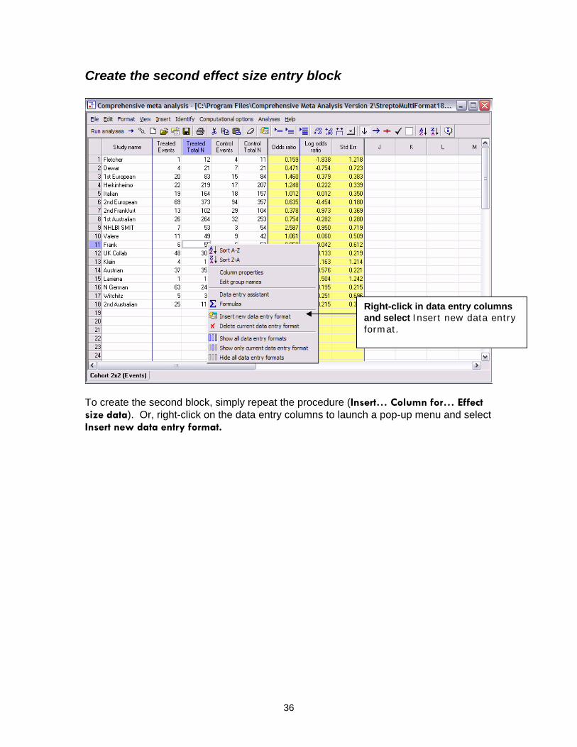
Create the second effect size entry block

Right-click in data entry columns and select Insert new data entry format.

To create the second block, simply repeat the procedure (Insert… Column for… Effect size data). Or, right-click on the data entry columns to launch a pop-up menu and select Insert new data entry format.

36

Select second effect size entry format

Choose format and click Finish.

Note that the Dichotomous (number of events) book icon remains open from the selection of the first effect size entry format.

In this example we want to create a block of columns to enter the odds ratio and confidence interval. Drill down in the hierarchy to select the following:

• Dichotomous (number of events)

• Computed effect sizes • Odds ratio and confidence limits

At this point, the Finish button will be activated. Click on it to create the columns for data entry.

37

Enter data for second effect size

Use these tabs to switch between formats.

Data are now entered in the second effect size block for the final four studies.

Effect size index results are automatically calculated and display in the yellow columns. Note that it is not necessary to enter both ‘Lower limit’ and ‘Upper limit’ values in this format. (If both are entered, the program will check to ensure that the values are consistent. For example, if the ‘Odds ratio’ is 1.000 and the ‘Lower limit’ is 0.500, the ‘Upper limit’ must be 2.000. Currently, the program allows a small margin for rounding error. (This margin value can be modified through the Computational options on the top menu).

Since there is now more than one format, the program has added a column to identify the format for each row. The formats, Cohort 2x2 (Events) and Odds ratio are inserted by the program automatically when the user enters data.

• Right-click on the data entry columns and select Show all data entry formats to modify the display. If you elect to Hide all data entry formats they can be re-displayed by right-clicking on the tab at the bottom of the screen.

• Right-click on the yellow columns and add “Risk ratio” as an index. As shown above,

this ratio will display for the first 18 studies (since it can be computed from the data provided) but not for the last four.

38

View analysis

For an analysis using odds ratios (as shown here), data from all studies would be available. Note that Events / Total counts display where relevant.

For an analysis using risk ratios, only data from the first 18 studies would be available, since the data from the last 4 studies cannot be used to compute a risk ratio.

39

Section 3. Working with moderator variables The program allows you to create two types of moderator variables which can then be used in the analysis. This chapter will describe the use of categorical moderators. (Chapter 9, on ‘Meta regression’, describes the use of numeric moderators.)

Once a categorical moderator variable is defined the user will be able to group by that variable. The program will also offer options for fixed effect, multiple mixed effect models, and a fully random effects model.

These options, still in development, are explained in this section.

By default, data sets are copied to C:\Program Files\Comprehensive Meta Analysis Version 2\Demo Files. The dataset used in this section is StreptoModerator.

40

Create the moderator column

Double-click here to launch the dialog.

Select Moderator and enter a variable name.

The program allows you to compare the effect size in two groups of outcomes. For example, you may want to compare the effect size in studies using acute patients with the effect size in studies using chronic patients. In order to group the studies for such a comparison you must first set up a moderator variable column.

• Double-click on an unassigned column header to launch the column format dialog.

The dialog allows you to select a column function, in this case Moderator, and to enter a variable name, in this case, ‘Patient Type’.

• Specify that the variable data type is Categorical. • Click on OK to create the moderator column and to begin data entry.

41

Enter moderator values

Enter values in this column.

The moderator values, either “Acute” or “Chronic”, are now entered for each study in the ‘Patient Type’ column. The toggle button circled above allows you to switch to dropdown data entry, so that you can enter “Acute” or “Chronic” by typing only the first letter of either word.

42

Select a grouping variable

Click on the Computational options… Group by selection to launch the Group by dialog.

Select ‘Patient Type’ as the moderator.

In this example we will run an analysis within each patient level and an ‘overall analysis’ across all levels. Because the second box is checked, within-groups and between-groups heterogeneity values will be provided in the appropriate view (described below).

43

Run Group by… analysis

Summary for each group

Summary across all studies

The pale yellow rows provide summaries at each level, “Acute” and “Chronic”. The bold yellow ‘Overall’ row provides a summary for both levels.

44

Select a computational model Select View… Analysis to switch to the ‘Analysis’ screen.

Click on the Computational options… Mixed and random effects options selection to launch the dialog.

The options selected here will determine the model to be used for calculating group summary and overall summary values.

45

View additional statistics by group

Click on the Next table toggle option to display this window, showing additional statistics at each level and overall. The within-groups and between-groups heterogeneity values are also broken out. In the report pop-up is a brief explanation of the assumptions which underlie the selected models. The circled icon allows the user to display and hide the report pop-up.

46

Recode column values

The program offers a set of options for making general changes to the contents of a column. To make such changes to the ‘Patient Type’ column, you would double-click on the column header and select the Values tab in the dialog, as shown above.

You could then do the following:

• Remove selected values or Remove unused values. The removed values will no longer appear in the ‘Patient Type’ data entry dropdown.

• Copy values from. Copy values from another column so that they are available for selection in the ‘Patient Type’ data entry dropdown.

• Recode. Modify all instances of a value in the column. As an example, the following image shows how to change “Chronic” and “Acute” to “Chronic condition” and “Acute condition” throughout the ‘Patient Type’ column.

47

Click on Apply recode to replace the current column values with new values.

48

Section 4. Subgroups within studies In the main example summary data were recorded for the full sample in each study.

The program also allows the user to record data for subgroups within the study. For example, if there were reason to believe that the treatment effect varied as a function of gender, some (or all) studies might report the treatment effect separately for males and females.

In this case we would enter the data for each study on two rows – one for males and one for females.

In the analyses we would want to do some (or all) of the following:

• Using subgroup as the unit of analysis, run an analysis grouped by gender. This

would report the treatment effect for each gender, and assess the impact of gender on the treatment effect. We could also run an overall analysis.

• Using subgroup as the unit of analysis, run the analysis for either gender alone. • If it emerged that the treatment effect was comparable for males and females, the

researcher might elect to use study as the unit of analysis. This would require having the program collapse the rows for male and female within each study, and impute the values for the full group.

The program offers all of these options, which are outlined in this section.

By default, data sets are copied to C:\Program Files\Comprehensive Meta Analysis Version 2\Demo Files. The dataset used in this section is StreptoSubGroups.

49

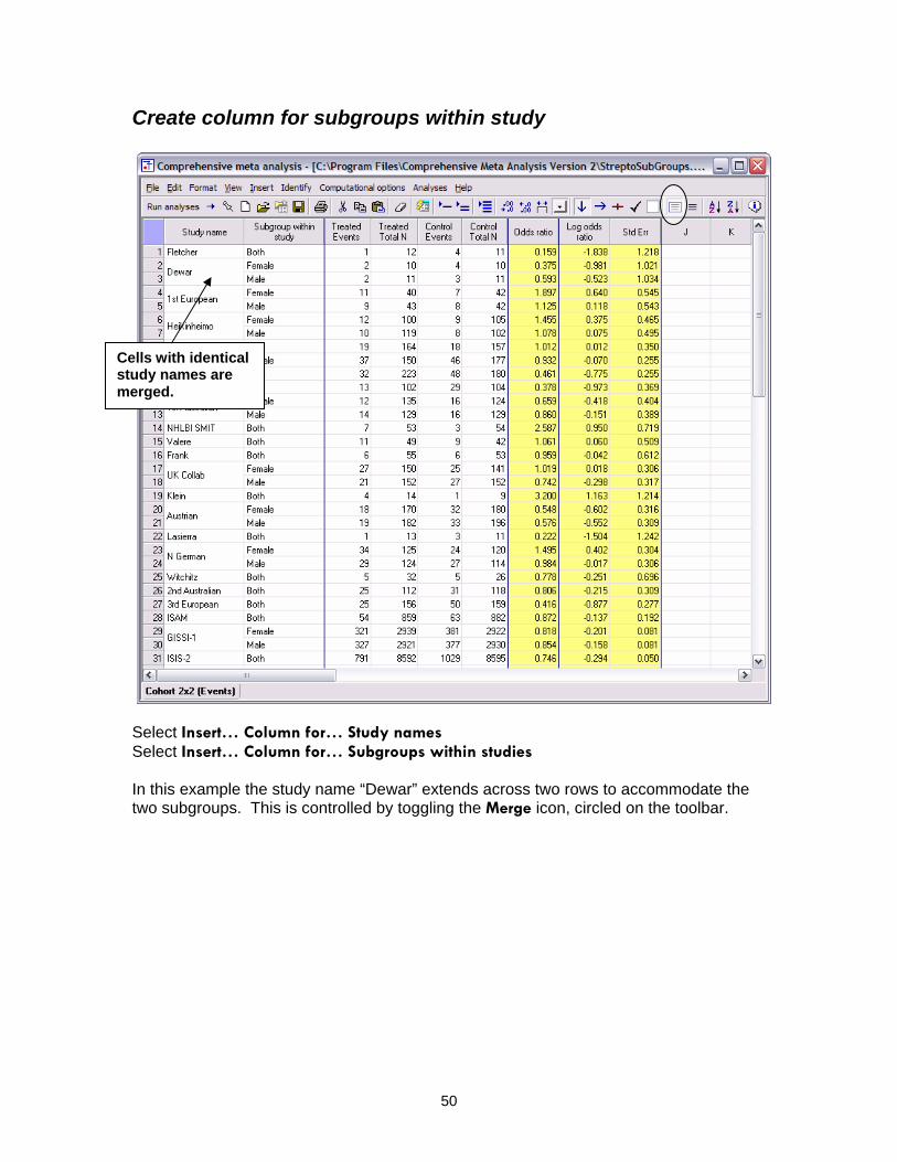
Create column for subgroups within study

Cells with identical study names are merged.

Select Insert… Column for… Study names Select Insert… Column for… Subgroups within studies In this example the study name “Dewar” extends across two rows to accommodate the two subgroups. This is controlled by toggling the Merge icon, circled on the toolbar.

50

View analysis

Right-click here and choose Select by Subgroup within study to launch the dialog.

At the top of the dialog box, use check-marks to select which subgroups should be included in the analysis.

At the bottom of the dialog box, specify whether to use subgroup within study or study as the unit of analysis.

If subgroup is the unit of analysis, you may use the Group by button and run an analysis using gender as the moderator variable.

51

Use study as the unit of analysis

This analysis is run according to the selection: Use study as the unit of analysis.

Those studies with multiple subgroups display the term ‘Combined’ in the Subgroups within study column. Those studies that had initially been entered on one line as “Both” are displayed here as they had been entered, since there is no imputation required.

52

Multiple sets of subgroups

The program can accommodate studies which report treatment effect for more than one set of subgroups.

For instance, certain studies may report results by age level as well as by gender. Such subgroup sets are not independent; they share subjects. It is therefore necessary to limit the analysis to one set at a time.

As an example, to accommodate both age and gender subgroup sets, first enter the data as shown above.

To merge contiguous study names, click on the circled icon.

53

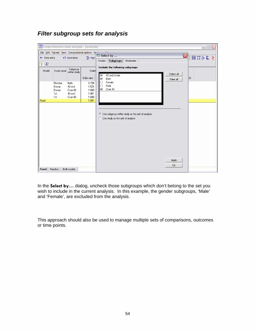
Filter subgroup sets for analysis

In the Select by… dialog, uncheck those subgroups which don’t belong to the set you wish to include in the current analysis. In this example, the gender subgroups, ‘Male’ and ‘Female’, are excluded from the analysis.

This approach should also be used to manage multiple sets of comparisons, outcomes or time points.

54

Section 5. Multiple outcomes within studies In the initial example, we assumed that we needed to record one treatment effect for each study. However, there are situations where the user will want to record more than one treatment effect per study. These are outlined here.

• More than one comparison per study. Assume that some (or all) studies report the

treatment effect for Control vs Treatment-A and also Control vs Treatment-B. We would want to record each treatment effect, and then use this information in the analysis.

• More than one outcome per study. Assume that some (or all) studies report the

treatment effect for more than one dependent variable – for example, the impact of the treatment in preventing myocardial infarction and also its impact in preventing death. We may want to run one analysis for the first outcome and a separate analysis for the second.

• More than one time point. Assume that studies record the treatment effect at six

months and also at one year. We would want to record both, and then run the analysis on one or the other.

This synopsis is meant only to introduce the topic of multiple, non-independent data points. The ability of the program to work with these will be much more extensive than alluded to here.

In this example we limit ourselves to the simplest case, where the user selects one item of information from each study. This example focuses on outcomes, but the same options are available for comparisons or time points.

A separate section in this document addresses the use of multiple subgroups within studies.

By default, data sets are copied to C:\Program Files\Comprehensive Meta Analysis Version 2\Demo Files. The dataset used in this section is StreptoOutcomes.

55

Create the outcome column

First, insert a column for Study names. Then, insert a column for Outcome name.

Select Insert… Column for… Study names. Select Insert… Column for… Outcome name.

56

Enter outcome values

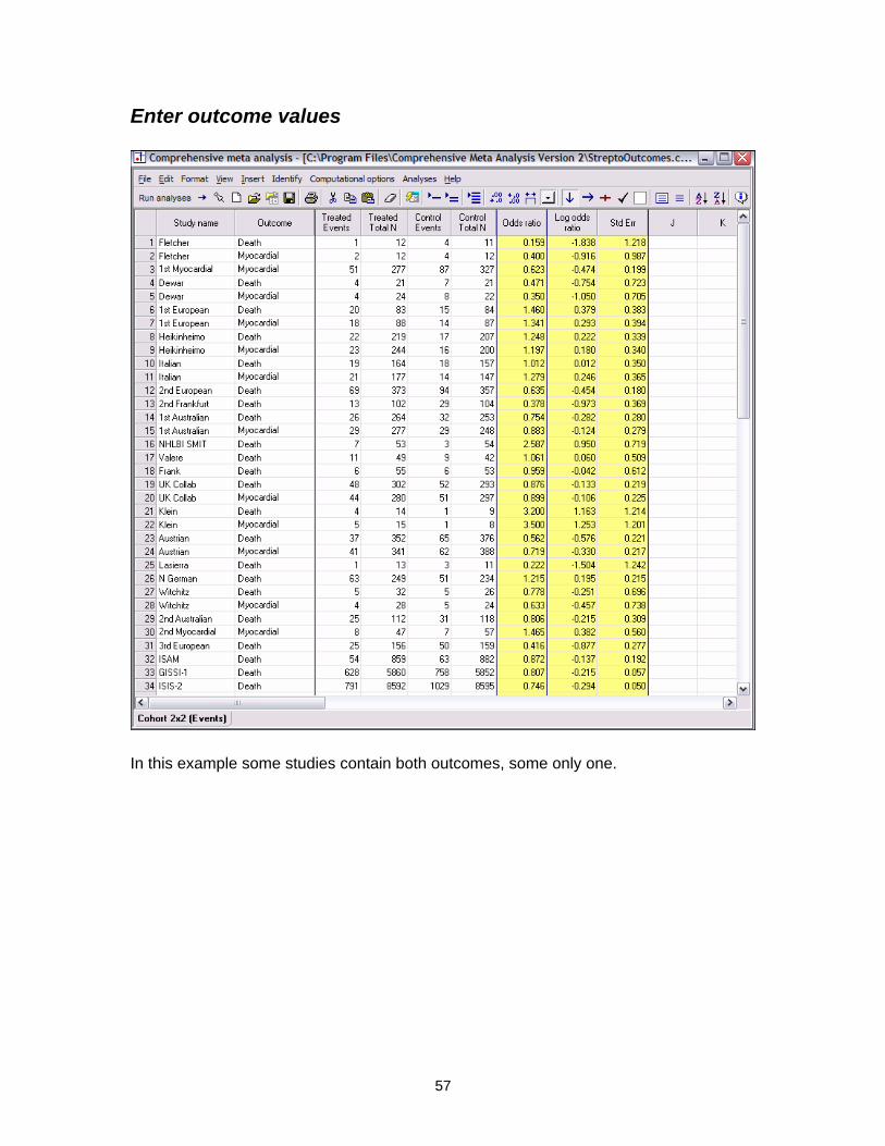
In this example some studies contain both outcomes, some only one.

57

View analysis for one outcome

Double-click here to launch the dialog box.

Note that only one outcome displays in the Outcome column. That is the only outcome selected in the dialog.

With the settings provided in the Group by dialog, you can also produce analyses which group results by outcome across multiple outcomes.

58

Section 6. Importing data from other programs The data entry screen is a spreadsheet, and the user may cut and paste data from most programs, such as Excel, STATA, or SPSS, which are able to display the data in spreadsheet form.

To import data • Switch to the other program and display the data in the Grid View. • Copy the data to the Windows clipboard (CTRL-C) • Switch to this program and paste the data into the spreadsheet (CTRL-V) One step remains – the user must identify the column with the study names, and the columns with the effect size data. Instructions follow.

By default, data sets are copied to C:\Program Files\Comprehensive Meta Analysis Version 2\Demo Files. The Excel spreadsheet is BCG.xls. The CMA data file is BCG.cma.

59

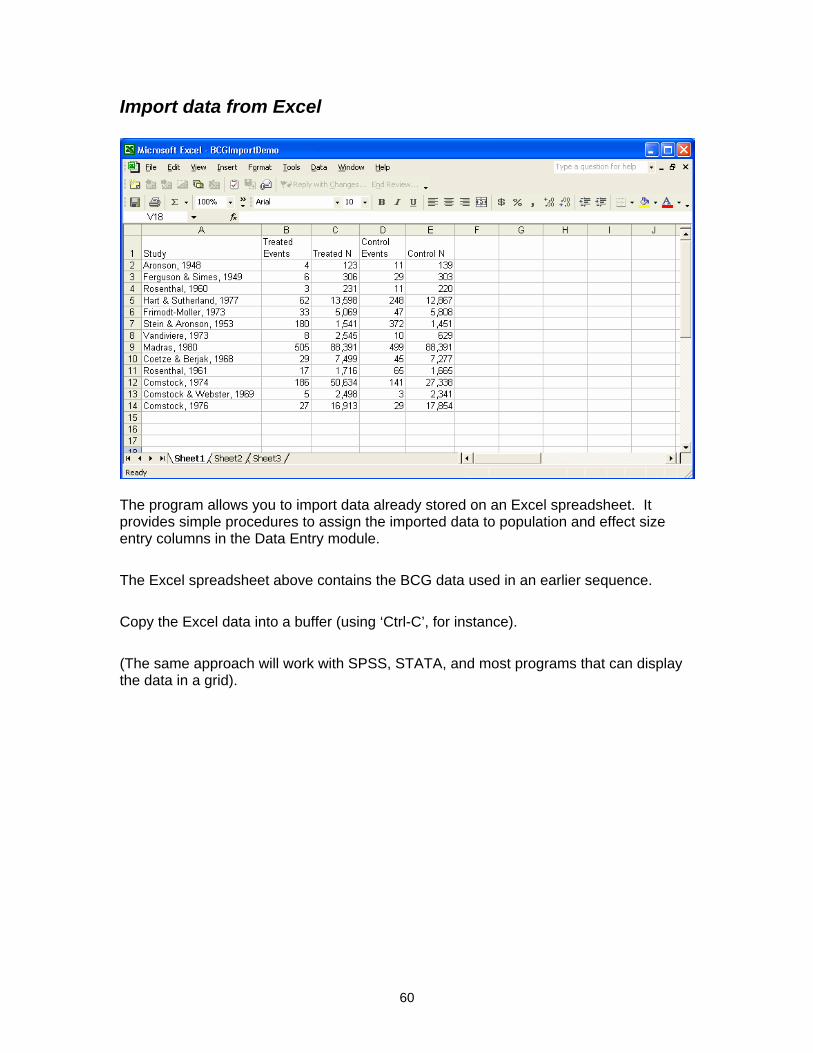
Import data from Excel

The program allows you to import data already stored on an Excel spreadsheet. It provides simple procedures to assign the imported data to population and effect size entry columns in the Data Entry module.

The Excel spreadsheet above contains the BCG data used in an earlier sequence.

Copy the Excel data into a buffer (using ‘Ctrl-C’, for instance).

(The same approach will work with SPSS, STATA, and most programs that can display the data in a grid).

60

Paste data into the data entry module

Switch to Comprehensive Meta Analysis and use ‘Ctrl-V’ to paste the data into the spreadsheet.

61

Assign column header titles

In this example the top row of the data file contains titles (“Study”, etc). Click on Format and select Use first row as labels.

62

Assign a ‘Study name’ column

Double-click on column header to launch the dialog.

Double-click on the header for the “Study” column and identify the function of the column as ‘Study name’.

Note: This is required even though the column is named “Study”.

63

Identify the effect size columns

Select Identify… Column for… Effect size data.

Select Identify… Column for… Effect size data Be sure to use Identify to identify the existing columns, rather than Insert, which would create new columns.

The program will launch the effect size entry wizard. The function is identical to that for creating a new spreadsheet, until the last panel of the wizard. There, instead of creating the columns, the program will ask you to identify their location.

64

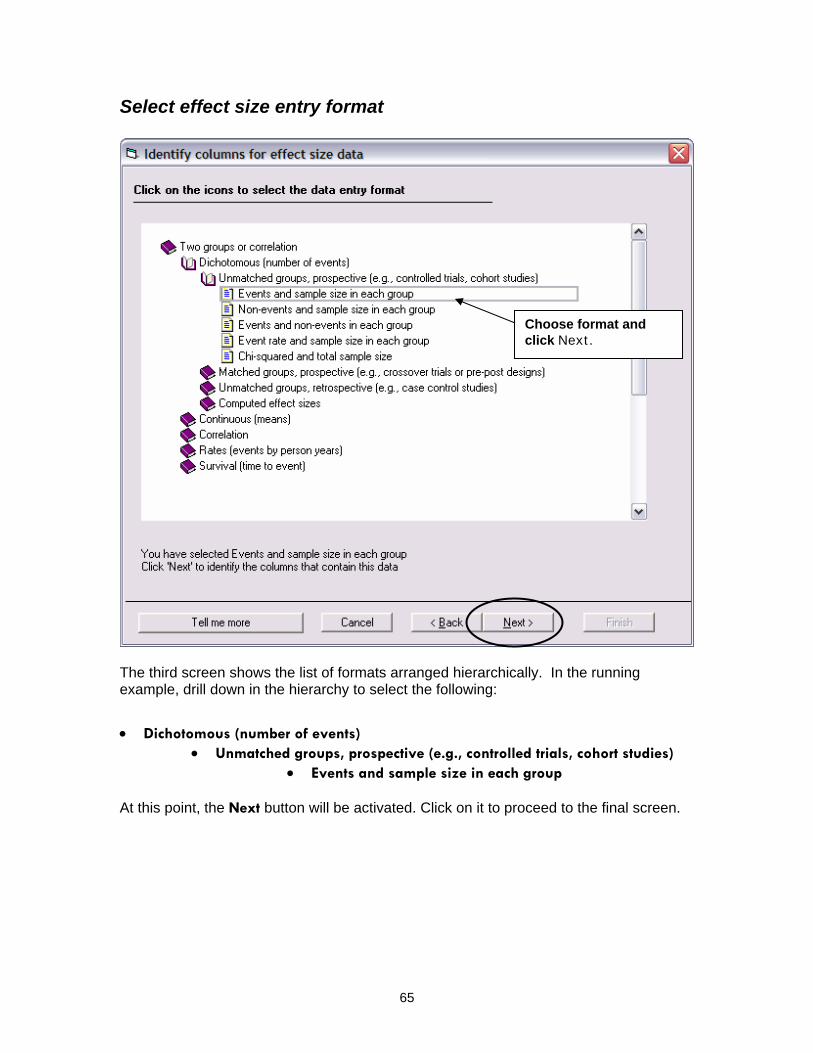
Select effect size entry format

Choose format and click Next.

The third screen shows the list of formats arranged hierarchically. In the running example, drill down in the hierarchy to select the following:

• Dichotomous (number of events)

• Unmatched groups, prospective (e.g., controlled trials, cohort studies) • Events and sample size in each group

At this point, the Next button will be activated. Click on it to proceed to the final screen.

65

Assign effect size entry columns

Click here to assign the column with the ‘Treated Events’ title to the corresponding effect size entry column.

Select a column title from the dropdown in order to assign that column’s data to the corresponding effect size entry column.

Then, click Finish.

66

All imported columns assigned

The study names and effect size entry columns are now appropriately assigned. The effect size results are automatically calculated and display in the yellow columns.

At this point, the program behaves exactly as if the spreadsheet had been created from scratch.

67

Importing data with multiple outcomes per row

Data are often stored as above, one row per study, with multiple outcomes per row. The following steps explain how to export this data and format it so that it fits the structure of the Data Entry module.

First, paste the Excel data directly onto the Data Entry spreadsheet. Then cut and paste the data into vertical blocks, one for each outcome.

68

• Click on Identify… Column for… Study names to assign that column.

• Click on Insert… Column for… Outcome names to create that column. Populate the column with the appropriate outcome value, “Verbal Score” or “Math Score”.

• Identify the effect size format columns via Identify… Columns… For effect size data. Within the effect size identification wizard, select the appropriate format, in this case: Continuous (means)… Unmatched groups…Cohen's d (standardized by pooled within-groups SD) and sample size

69

Click on the study names column and then on the ascending sort icon, circled above. The data are now sorted by study name so that multiple outcomes for a given study display on contiguous rows.

The Merge icon has been clicked so that contiguous study names are merged.

(Note that ascending and descending sorts can be performed on any column. To order studies by date, you could enter study dates into an unassigned column or a moderator column and then sort on that column.)

70

Import data with multiple effect size entry formats

When the study results to be imported require multiple entry formats, paste the data into the Data Entry module as above, with the second format’s columns to the right of the first format’s columns. To assign the imported data shown above, follow these steps:

• Click on Format and select Use first row as labels (keep in mind that the column names must be unique).

• Double-click on the header for the “Study” column and identify the function of the column as ‘Study name’.

• For rows 2 – 19, select Identify… Column for… Effect size data and assign the data columns to the Events and sample size in each group entry format.

• For rows 20 – 23, select Identify… Column for… Effect size data and assign the data columns to the Odds ratio and confidence limits entry format. (Note that Upper limits values are missing from the pasted data. The Identify… function will automatically create an empty Upper limits column.)

The data will display, fully formatted as it does in chapter 2 (which discusses multiple data entry formats).

71

Section 7. Saving and loading files This section shows how to save and reload your data sets.

72

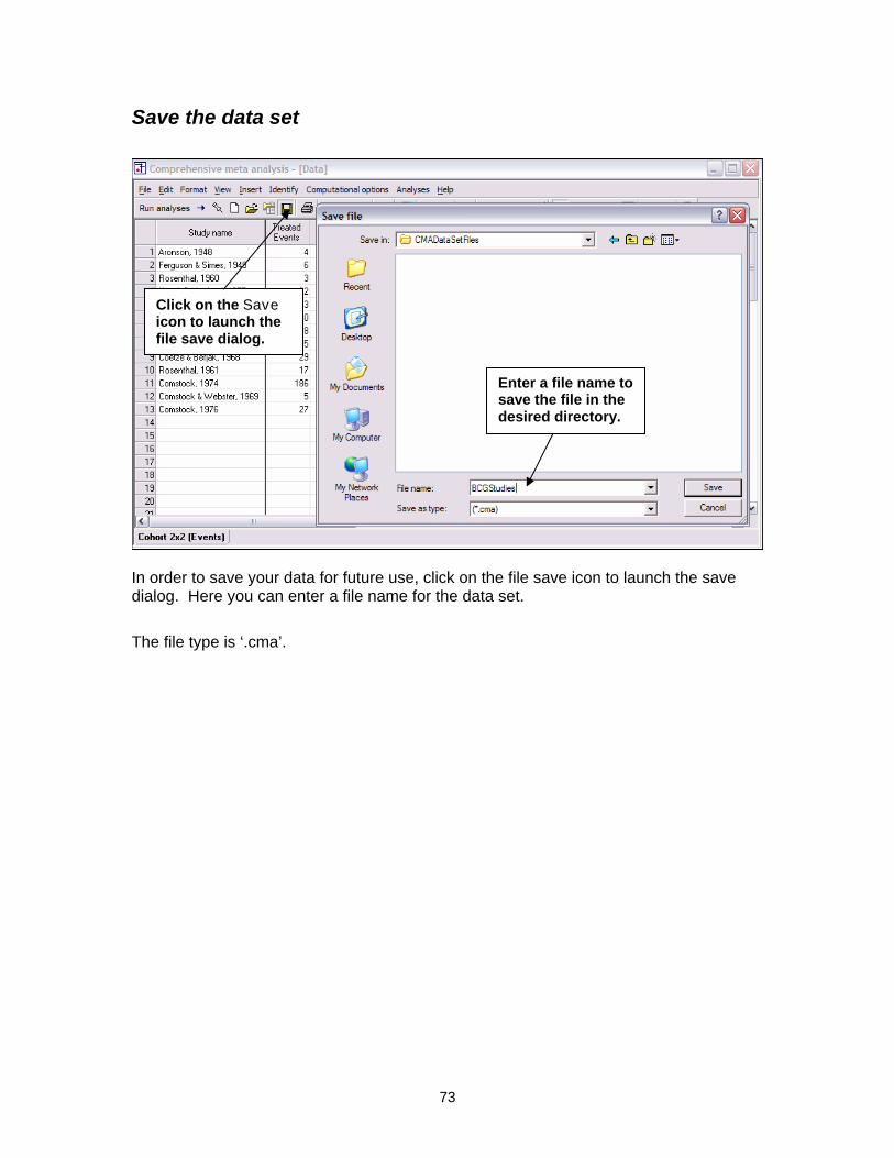
Save the data set

Click on the Save icon to launch the file save dialog.

Enter a file name to save the file in the desired directory.

In order to save your data for future use, click on the file save icon to launch the save dialog. Here you can enter a file name for the data set.

The file type is ‘.cma’.

73

Open and load the saved data set

Click on File and Open to launch the file open dialog.

Navigate to the desired directory. All CMA files will display.

Use this file open dialog to locate, select and download previously saved data sets.

74

Section 8. Publication-quality graphics The program enables you to create and easily format publication-quality graphics. The Graphics module will allow you to print the graphics, export them to common presentation formats, such as Word or PowerPoint, or save them in formats such as “PDF” or “WMF”.

Please note that, in this release, only the exports to Word and PowerPoint and the save as “WMF file” are operational.

75

Modify analysis display

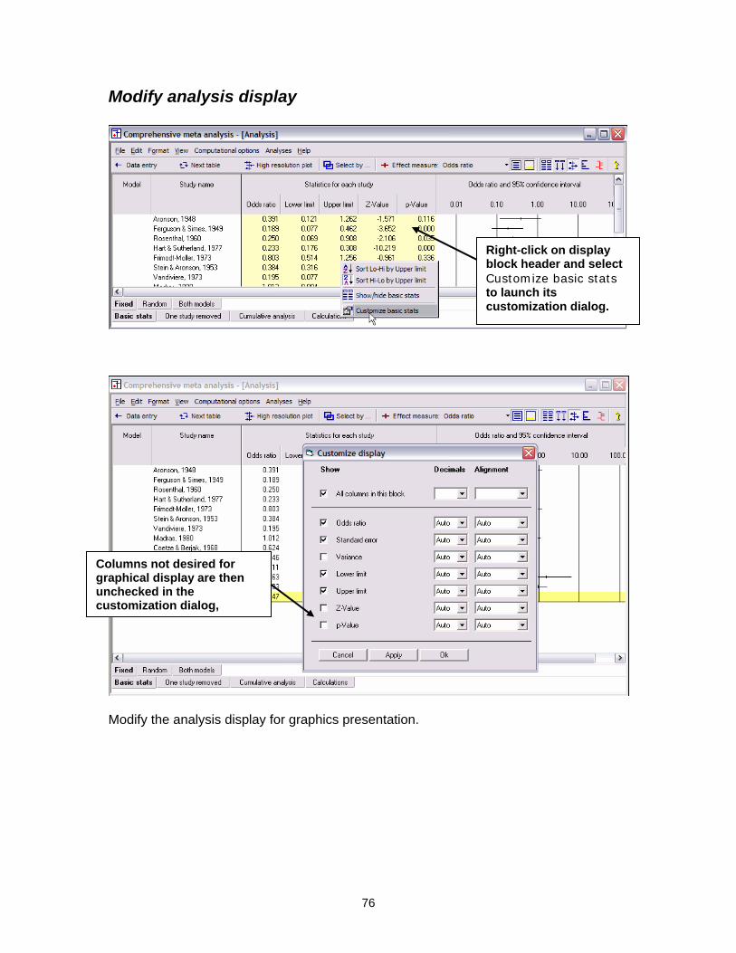
Right-click on display block header and select Customize basic stats to launch its customization dialog.

Columns not desired for graphical display are then unchecked in the customization dialog,

Modify the analysis display for graphics presentation.

76

Launch graphics module

Click on View… High resolution plot.

77

Format graphics display

The graphic first displays in a default mode. Right-clicking on any segment of the display will drop down a list of context-sensitive formatting options. Clicking on the Format icon circled on the toolbar will drop down the list below, displaying a more comprehensive set of adjustment options.

78

Change computational model

Click on the Computational options button to vary the model used for determining summary results (Fixed effect, Random effects or Both models).

In the Forest plot the studies are represented by symbols whose area is proportional to the study’s weight in the analysis.

79

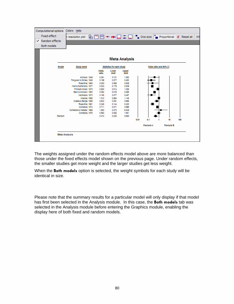
The weights assigned under the random effects model above are more balanced than those under the fixed effects model shown on the previous page. Under random effects, the smaller studies get more weight and the larger studies get less weight.

When the Both models option is selected, the weight symbols for each study will be identical in size.

Please note that the summary results for a particular model will only display if that model has first been selected in the Analysis module. In this case, the Both models tab was selected in the Analysis module before entering the Graphics module, enabling the display here of both fixed and random models.

80

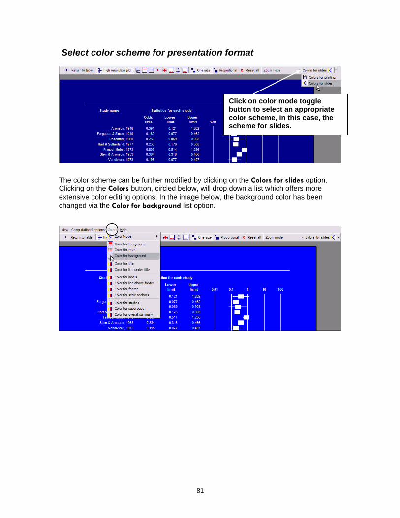
Select color scheme for presentation format

Click on color mode toggle button to select an appropriate color scheme, in this case, the scheme for slides.

The color scheme can be further modified by clicking on the Colors for slides option. Clicking on the Colors button, circled below, will drop down a list which offers more extensive color editing options. In the image below, the background color has been changed via the Color for background list option.

81

Format text

To change text and fonts in header, footer and plot labels, right-click on each to launch the context-sensitive formatting pop-ups.

82

Export to file

Click on File to select an option for printing, copying, exporting or saving the graphic display.

In this case, the graphics image has been exported to PowerPoint which opens automatically and displays the converted graphic.

83

Section 9. Meta regression This module allows you to run a regression analysis to estimate the impact of continuous study moderators on overall heterogeneity.

By default, data sets are copied to C:\Program Files\Comprehensive Meta Analysis Version 2\Demo Files. The dataset used in this section is BCGLatitude.

84

Define a moderator

In order to perform a meta-regression you must first create a continuous moderator and define it as decimal or numeric. In this example, using the BCGLatitude data set, the impact of a study location’s latitude will be examined.

85

Launch the Meta regression module

Select Meta regression from the Windows option dropdown. The effect size index used in the Analysis module (log odds ratio here) will also be used in the regression analysis.

86

Select the moderator

Select the moderator to be used as the covariate in the regression analysis. The dropdown list will contain all available numeric moderators.

87

View the regression scatter plot

After selection of the moderator, the program displays the regression line and scatter plot of studies. In the default presentation, all studies are represented by circles of identical size, regardless of their individual weighting in the analysis. (Note the circled One size option.)

88

Adjust scatter plot display

Click on the Proportional option to view the same graph, but this time with each study represented by a circle proportional to its weight in the analysis. This view identifies which studies have the greatest impact on the slope of the regression line.

89

Select the regression model

Click on the Computational options button and select from among the three available models, Fixed effect, Method of moments, Unrestricted ML (maximum likelihood). Each of the displays in this module reflects the model chosen. Basic meta regression results are given in the display above, which is invoked by clicking on the Table toggle button.

90

View iterations

Click on View… Show Iterations to display the iterations needed by the unrestricted maximum likelihood algorithm to bring successive ‘Tau-squared’ variance values into virtual convergence, at which point the final meta-regression values have been attained. As the above display makes clear, the model required 38 iterations in this case to arrive at final results.

91

View data and residuals

Click on View… Show Calculations to display the calculations involved in producing the regression analysis results.

92

Section 10. Publication Bias This module offers multiple methods for detecting the presence of publication bias and assessing its impact on the analysis.

By default, data sets are copied to C:\Program Files\Comprehensive Meta Analysis Version 2\Demo Files. The dataset used in this section is StreptoModerator.

93

Funnel plot

To launch the Publication Bias module from the Analysis module, click on Analyses… Publication bias. The default display, a funnel plot, has two modes, one which plots a study’s effect size against its standard error (above) and another which plots effect size against precision, the inverse of standard error (next page). Toolbar icons allow the user to alter the color scheme and other plot attributes.

94

Click here to switch between plot modes (standard error and precision).

Click here to switch model between fixed effect and random effects.

The plot by precision is the traditional form. Note that large studies appear toward the top of the graph, and tend to cluster near the mean effect size. Smaller studies appear toward the bottom of the graph, and (since there is more random variation in the small studies) are dispersed across a range of values. This pattern tends to resemble a funnel, which is the basis for the plot’s name. In the absence of publication bias the studies will be distributed symmetrically about the combined effect size. By contrast, in the presence of bias, the bottom of the plot would tend to show a higher concentration of studies on one side of the mean than the other. This would reflect the fact that smaller studies (which appear toward the bottom) are more likely to be published if they have larger than average effects, which makes them more likely to meet the criterion for statistical significance.

95

Duval and Tweedie’s trim and fill

The View option drops down a selection of methods for assessing publication bias, including the Trim and Fill procedure, shown here. Trim and Fill builds on the key idea behind the funnel plot; that in the absence of bias the plot would be symmetric about the summary effect. If there are more small studies on the right than on the left, the concern is that studies may be missing from the left. The Trim and Fill procedure imputes these missing studies, adds them to the analysis, and then re-computes the summary effect size. By default, the tool will look for missing studies to the left of the summary effect. The user can reverse the search direction by selecting the appropriate setting. The report icon (circled above) launches a description of the statistical test and an explanation of the actual results it yields. In our example there is one imputed missing study. In addition, the report tells us that: “Under the fixed effect model the point estimate and 95% confidence interval for the combined studies is -0.25556 (-0.32085, -0.19027). Using Trim and Fill the imputed point estimate is -0.25663 (-0.32190, -0.19136). Under the random effects model the point estimate and 95% confidence interval for the combined studies is -0.24513 (-0.36721, -0.12304). Using Trim and Fill the imputed point estimate is -0.24873 (-0.37160, -0.12587).”

96

To view Trim and Fill’s imputed studies on the funnel plot, click on the toggle icon circled above. In our example the data point for one imputed study is highlighted in black (near bottom left of plot).

97

Begg and Mazumdar rank correlation

Begg and Mazumdar’s rank correlation test reports the rank correlation (Kendall’s tau) between the standardized effect size and the variances (or standard errors) of these effects. Tau would be interpreted much the same way as any correlation, with a value of zero indicating no relationship between effect size and precision, and deviations from zero indicating the presence of a relationship. If asymmetry is caused by publication bias we would expect to see high standard errors (small studies) associated with larger effect sizes. If larger effects are represented by low values, tau would be positive, while if larger effects are represented by high values, tau would be negative. Since asymmetry could appear in the reverse direction, the significance test is two-sided. In our example Kendall's tau b (corrected for ties, if any) is -0.01732, with a 1-tailed p-value (recommended) of 0.45510 or a 2-tailed p-value of 0.91020. Note that the Next table button allows you to toggle among all the available publication bias tests.

98

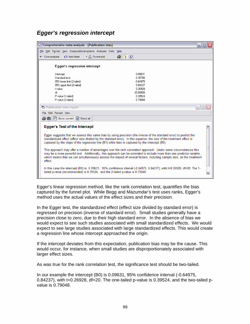
Egger’s regression intercept

Egger’s linear regression method, like the rank correlation test, quantifies the bias captured by the funnel plot. While Begg and Mazumdar’s test uses ranks, Egger’s method uses the actual values of the effect sizes and their precision. In the Egger test, the standardized effect (effect size divided by standard error) is regressed on precision (inverse of standard error). Small studies generally have a precision close to zero, due to their high standard error. In the absence of bias we would expect to see such studies associated with small standardized effects. We would expect to see large studies associated with large standardized effects. This would create a regression line whose intercept approached the origin. If the intercept deviates from this expectation, publication bias may be the cause. This would occur, for instance, when small studies are disproportionately associated with larger effect sizes. As was true for the rank correlation test, the significance test should be two-tailed. In our example the intercept (B0) is 0.09631, 95% confidence interval (-0.64975, 0.84237), with t=0.26928, df=20. The one-tailed p-value is 0.39524, and the two-tailed p-value is 0.79048.

99

Fail-safe N

Rosenthal’s Fail-safe N test computes the number of missing studies (with mean effect of zero) that would need to be added to the analysis to yield a statistically non-significant overall effect. The user can edit the Alpha and Tails parameters In our example Rosenthal’s fail-safe N is 113. This means that we would need to locate and include 113 'null' studies in order for the combined 2-tailed p-value to exceed 0.050. Put another way, there would be need to be 5.1 missing studies for every observed study for the effect to be nullified. The Orwin variant of this test addresses two problems with Rosenthal’s method; that it focuses on statistical rather than clinical significance, and that it assumes a nil overall effect in the missing studies. Orwin’s test allows you to select both the smallest effect value deemed to be clinically important and a value other than nil for the mean effect in the missing studies. To vary these values, edit the relevant parameters, which in our example are Criterion for a ‘trivial’ log odds ratio and Mean log odds ratio in missing studies. In our example Orwin’s fail-safe N is 18. This means that we would need to locate 18 studies with mean log odds ratio of 0.1 to bring the combined log odds ratio over -0.1 (see the Orwin parameter settings in the image).

100

Section 11. Data Entry Templates This module describes the basic templates provided to facilitate data entry.

101

View templates

To expedite data entry, the program provides templates which contain pre-established columns for study names and commonly used entry formats. To view the templates, click on the option selected above in the Welcome dialog.

102

Select a template

Select the template which fits your data format. Note the file extension of ‘cmt’, indicating template. Additional templates will be included in future releases.

103

Enter data

The data entry module displays the pre-established columns associated with the selected template.

Enter data, modify as desired, and save as a normal data set (with extension ‘cma’.) The newly created data set can be re-opened and modified. The template remains intact and can be re-selected to begin entry of a new data set.

104