COMPREHENSIVE D P F MODELING, FORMULATION, SOLUTION ALGORITHMS AND ANALYSIS · ·...

COMPREHENSIVE DISTRIBUTION POWER FLOW: MODELING, FORMULATION, SOLUTION

ALGORITHMS AND ANALYSIS

A Dissertation

Presented to the Faculty of the Graduate School

of Cornell University

in Partial Fulfillment of the Requirements for the Degree of

Doctor of Philosophy

by

Ray Daniel Zimmerman

January 1995

COMPREHENSIVE DISTRIBUTION POWER FLOW: MODELING, FORMULATION, SOLUTION ALGORITHMS AND ANALYSIS

Ray Daniel Zimmerman, Ph.D.

Cornell University 1995

The objective of this work was to develop a formulation and an effi-

cient solution algorithm for the distribution power flow problem which

takes into account the detailed and extensive modeling necessary for use in

the distribution automation environment of a real world electric power dis-

tribution system.

The formulations for the three classes of existing algorithms for radial

systems were generalized and were extended to handle the comprehensive

modeling already presented in the context of more traditional but less effi-

cient methods, such as Newton-Raphson and Implicit Zbus Gauss. The

modeling includes unbalanced three-phase, two-phase, and single-phase

branches, constant power, constant current, and constant impedance loads

connected in wye or delta formations, cogenerators, shunt capacitors, line

charging capacitance, switches, and three-phase transformers of various

connection types.

The three classes of algorithms explored are: network reduction meth-

ods, backward/forward sweep methods, and fast decoupled methods.

Within each of the three classes, new algorithms were developed and exist-

ing methods were extended to include the comprehensive modeling of the

general formulation. Proofs of convergence for the backward/forward

sweep and fast decoupled methods are also provided.

In addition to the radial algorithms, the compensation method used to

handle weakly meshed systems was generalized to encompass three-phase

networks with loops, multiple sources, and three-phase PV buses. This

compensation method can be applied in conjunction with any of the radial

power flow solvers. Termination of the radial solver, at each iteration, is

based on an adaptive criterion. A generalized correction step for the com-

pensation method was also developed.

All of the proposed methods were evaluated and compared on various

test systems based on data from real distribution systems. The test sys-

tems range in size from 63 buses to over 1000 buses. The most efficient

algorithm in each class was shown to require significantly less computa-

tion than both the Newton-Raphson and the Implicit Zbus Gauss methods,

with the backward/forward sweep and fast decoupled methods typically

showing an improvement of more than a factor of three.

iii

BIOGRAPHICAL SKETCH

Ray Daniel Zimmerman was born in Ephrata, PA on December 17,

1965. Four years later he moved with his family to a chicken farm in rural

Lancaster County, PA, where he lived until he began studying Electrical

Engineering in September of 1984. As an undergraduate at Drexel Univer-

sity in Philadelphia, PA, he participated in a cooperative education pro-

gram which involved working for six month periods at each of the following

companies: IBM Corporation, Research Triangle Park, NC, Evaluation

Associates, Bala Cynwyd, PA, and UNISYS Corporation, Tredyffrin, PA.

He received a Bachelor of Science degree in Electrical Engineering from

Drexel University in June, 1989. In August of

the same year he began graduate studies in

Electrical Engineering at Cornell University in

Ithaca, NY, where he received a Master of Sci-

ence degree in May, 1992, in the area of network

reconfiguration in electric power distribution

systems.

iv

to my wife, Esther

and my daughter, Ana

v

ACKNOWLEDGMENTS

Pero habiendo obtenido auxilio de Dios, persevero hasta el día de hoy. — Hechos 26:22

I would like to express my appreciation to my advisor, Dr. Hsiao-Dong

Chiang, for his support and direction for this work. I would also like to

thank Dr. James S. Thorp and Dr. Lloyd N. Trefethen for serving on my

committee. My appreciation also goes to Gary Darling of New York State

Gas & Electric and Matt Downey of Rochester Gas & Electric for providing

the data used for testing the methods developed in this work.

Several friends have been helpful throughout the various stages of

this work, whether through discussions of technical issues or simply with

helpful perspective on the process of getting a doctorate. In particular, I

would like to acknowledge Guerney Hunt, Jen-Lun Yuan, Yi-Jen Chiu,

Jianzhong Tong, and Karen Nan Miu. A special thanks to Karen for taking

the time to read this dissertation and make helpful comments to improve

its readability. I would also like to express my appreciation to Ernie for his

help in proofreading.

Most of all, I appreciate the constant support of my family, especially

during the final months of writing. Quisiera agradecer primero a Esther

por su amor y apoyo constante. Y gracias, Anita, por el ánimo que me das

solo verte crecer cada día. Gracias también por ser la compañerita de

mamá durante este tiempo difícil.

vi

TABLE OF CONTENTS

ABSTRACT

BIOGRAPHICAL SKETCH ...............................................................................................iiiACKNOWLEDGMENTS .....................................................................................................vTABLE OF CONTENTS ................................................................................................... viLIST OF TABLES..............................................................................................................xLIST OF FIGURES ......................................................................................................... xii

1 Introduction 11.1 Background.....................................................................................................11.2 Objectives and Contributions..........................................................................3

2 Basic Problem Framework 72.1 Mathematical Notation....................................................................................72.2 Bus and Lateral Indexing................................................................................8

2.2.1 Indexing Scheme.................................................................................92.2.2 Indexing Implementation..................................................................11

2.2.2.1 Connectivity Data Structures................................................112.2.2.2 Breadth-First Search .............................................................12

2.3 Basic System Model .....................................................................................152.3.1 Voltage and Current/Power Flow Update for Branch k ...................182.3.2 Application of KCL ..........................................................................19

3 Detailed Component Models 213.1 Load Model...................................................................................................23

3.1.1 Admittance Matrix for the Load .......................................................263.1.2 Current and Power Injected by the Load ..........................................27

3.2 Shunt Capacitor Model .................................................................................283.3 Cogenerator Model .......................................................................................293.4 Distribution Line Model ...............................................................................313.5 Switch Model................................................................................................333.6 Transformer Model.......................................................................................34

3.6.1 Class A: Primary and Secondary both Grounded or both Ungrounded ..........................................35

3.6.2 Class B: Grounded Primary—Ungrounded Secondary ....................353.6.3 Class C: Ungrounded Primary—Grounded Secondary ....................39

vii

4 Network Reduction Power Flow Algorithms for Radial Systems (NR-PARS) 42

4.1 Detailed Solution Algorithm.........................................................................434.1.1 Linearization .....................................................................................444.1.2 Build Driving Point Equivalents.......................................................454.1.3 Calculate Voltages and Currents.......................................................494.1.4 Termination Criterion .......................................................................51

4.2 Implementation .............................................................................................514.2.1 Linearity Check.................................................................................514.2.2 Improved Line Update......................................................................524.2.3 Storage of Intermediate Variables ....................................................52

4.3 Variations......................................................................................................534.4 Convergence Analysis ..................................................................................554.5 Comments .....................................................................................................55

5 Backward/Forward Sweep Power Flow Algorithms for Radial Systems (BFS-PARS) 57

5.1 Detailed Solution Algorithm.........................................................................585.1.1 Backward Sweep...............................................................................605.1.2 Forward Sweep .................................................................................625.1.3 Termination Criterion .......................................................................65

5.2 Implementation .............................................................................................665.2.1 Class B Transformers........................................................................66

5.2.1.1 Backward Sweep...................................................................665.2.1.2 Forward Sweep .....................................................................67

5.2.2 Class C Transformers........................................................................695.2.2.1 Forward Sweep .....................................................................695.2.2.2 Backward Sweep...................................................................70

5.3 Variations......................................................................................................725.3.1 VI-VI-PARS .......................................................................................725.3.2 VS-VS-PARS......................................................................................735.3.3 V-VI-PARS ........................................................................................755.3.4 V-VS-PARS........................................................................................755.3.5 VI-I-PARS .........................................................................................765.3.6 VS-S-PARS ........................................................................................765.3.7 V-I-PARS...........................................................................................765.3.8 V-S-PARS ..........................................................................................77

5.4 Convergence Analysis ..................................................................................775.5 Comments .....................................................................................................83

viii

6 Fast Decoupled Power Flow Algorithms for Radial Systems (DePARS) 846.1 Detailed Solution Algorithm.........................................................................85

6.1.1 Reduced Power Flow Equations.......................................................876.1.1.1 Single Feeder ........................................................................886.1.1.2 General Radial Structure.......................................................896.1.1.3 Class B and Class C Transformers........................................93

6.1.2 Update of Independent Variables......................................................946.1.2.1 Structure of the System Jacobian..........................................956.1.2.2 Numerical Properties of the System Jacobian ....................1006.1.2.3 Transformers.......................................................................1036.1.2.4 Solving for the Update........................................................107

6.1.3 Termination Criterion .....................................................................1076.2 Implementation ...........................................................................................1096.3 Variations....................................................................................................110

6.3.1 VI-DePARS .....................................................................................1116.3.2 VS-DePARS.....................................................................................1116.3.3 I-DePARS ........................................................................................112

6.3.3.1 Reduced Power Flow Equations.........................................1136.3.3.2 Update of the Independent Variables..................................1166.3.3.3 Implementation ...................................................................120

6.3.4 S-DePARS .......................................................................................1226.4 Convergence Analysis ................................................................................1236.5 Comments ...................................................................................................126

7 Power Flow Algorithms for Weakly Meshed Systems (PAWMS) 1277.1 Detailed Solution Algorithm.......................................................................128

7.1.1 Loop Breakpoint Creation...............................................................1307.1.2 Breakpoint Voltage Mismatch........................................................1317.1.3 Breakpoint Impedance Matrix ........................................................1327.1.4 Breakpoint Injections......................................................................1347.1.5 Multiple Sources.............................................................................1357.1.6 PV Buses.........................................................................................1367.1.7 Summary.........................................................................................1407.1.8 Termination Criterion .....................................................................140

7.2 Implementation ...........................................................................................1417.2.1 Modeling Limitations and Simplifying Assumptions.....................1417.2.2 Termination of Radial Power Flow.................................................141

7.3 Variations....................................................................................................1427.3.1 Power Injection for Loop Breakpoints............................................1437.3.2 Correction Step ...............................................................................144

7.4 Comments ...................................................................................................146

ix

8 Simulation Results 1488.1 Summary of Algorithms Tested..................................................................150

8.1.1 Newton-Raphson Method...............................................................1508.1.2 Implicit Zbus Gauss Method............................................................152

8.2 Description of Test Systems .......................................................................1548.3 Power Flow Algorithms for Radial Systems (PARS) .................................155

8.3.1 Effect of Load Model and Load Factor on Convergence ...............1608.3.2 Effect of System Size on Convergence...........................................163

8.4 Power Flow Algorithms for Weakly Meshed Systems (PAWMS)..............1658.4.1 Effect of PARS Termination Criterion on Convergence.................1668.4.2 Effect of Number of Loops on Convergence..................................1688.4.3 Effect of Load Model on Convergence...........................................171

8.5 Summary.....................................................................................................172

9 Conclusions 1759.1 Contributions...............................................................................................1759.2 Future Work................................................................................................178

BIBLIOGRAPHY ...........................................................................................................180

x

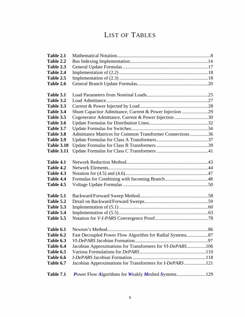
LIST OF TABLES

Table 2.1 Mathematical Notation..............................................................................8Table 2.2 Bus Indexing Implementation.................................................................14Table 2.3 General Update Formulas .......................................................................17Table 2.4 Implementation of (2.2) ..........................................................................18Table 2.5 Implementation of (2.3) ..........................................................................18Table 2.6 General Branch Update Formulas...........................................................20

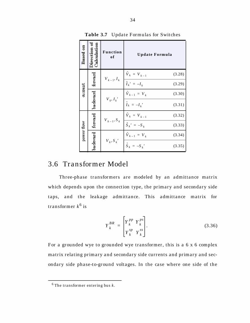
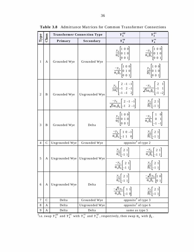
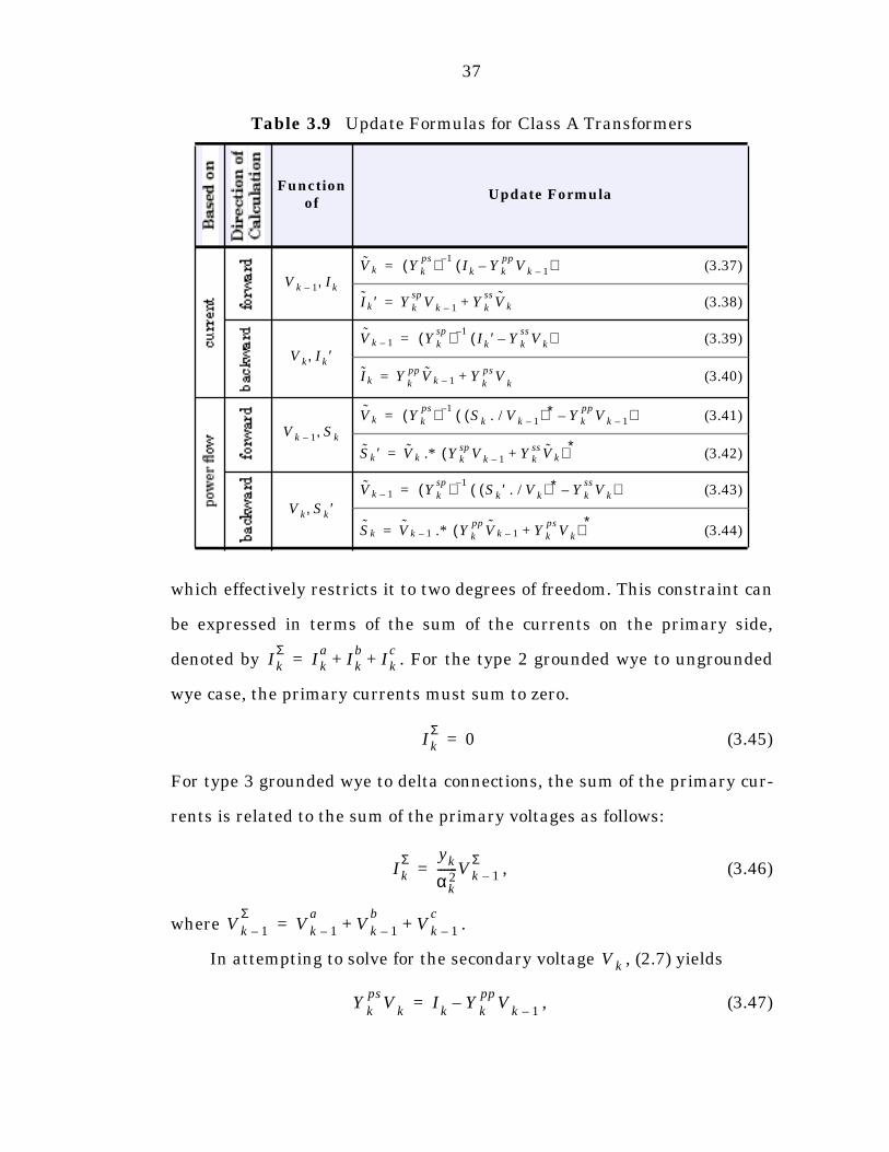
Table 3.1 Load Parameters from Nominal Loads...................................................25Table 3.2 Load Admittance.....................................................................................27Table 3.3 Current & Power Injected by Load.........................................................28Table 3.4 Shunt Capacitor Admittance, Current & Power Injection ......................29Table 3.5 Cogenerator Admittance, Current & Power Injection ............................30Table 3.6 Update Formulas for Distribution Lines.................................................32Table 3.7 Update Formulas for Switches................................................................34Table 3.8 Admittance Matrices for Common Transformer Connections ...............36Table 3.9 Update Formulas for Class A Transformers...........................................37Table 3.10 Update Formulas for Class B Transformers ...........................................39Table 3.11 Update Formulas for Class C Transformers ...........................................41

Table 4.1 Network Reduction Method....................................................................43Table 4.2 Network Elements...................................................................................44Table 4.3 Notation for (4.5) and (4.6).....................................................................47Table 4.4 Formulas for Combining with Incoming Branch....................................48Table 4.5 Voltage Update Formulas .......................................................................50

Table 5.1 Backward/Forward Sweep Method.........................................................58Table 5.2 Detail on Backward/Forward Sweeps.....................................................59Table 5.3 Implementation of (5.1) ..........................................................................60Table 5.4 Implementation of (5.5) ..........................................................................63Table 5.5 Notation for V-I-PARS Convergence Proof............................................78

Table 6.1 Newton’s Method....................................................................................86Table 6.2 Fast Decoupled Power Flow Algorithm for Radial Systems..................87Table 6.3 VI-DePARS Jacobian Formation.............................................................97Table 6.4 Jacobian Approximations for Transformers for VI-DePARS................106Table 6.5 Various Formulations for DePARS .......................................................110Table 6.6 I-DePARS Jacobian Formation .............................................................118Table 6.7 Jacobian Approximations for Transformers for I-DePARS ..................121

Table 7.1 Power Flow Algorithms for Weakly Meshed Systems........................129

xi

Table 8.1 Summary of Distribution Power Flow Algorithms...............................151Table 8.2 Summary of Test Systems ....................................................................154

Table 9.1 Summary of Radial Power Flow Algorithms........................................176

xii

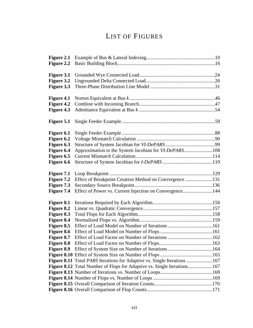
LIST OF FIGURES

Figure 2.1 Example of Bus & Lateral Indexing.......................................................10Figure 2.2 Basic Building Block..............................................................................16

Figure 3.1 Grounded Wye Connected Load.............................................................24Figure 3.2 Ungrounded Delta Connected Load........................................................26Figure 3.3 Three-Phase Distribution Line Model ....................................................31

Figure 4.1 Norton Equivalent at Bus k.....................................................................46Figure 4.2 Combine with Incoming Branch.............................................................47Figure 4.3 Admittance Equivalent at Bus k .............................................................54

Figure 5.1 Single Feeder Example ...........................................................................59

Figure 6.1 Single Feeder Example ...........................................................................88Figure 6.2 Voltage Mismatch Calculation ...............................................................90Figure 6.3 Structure of System Jacobian for VI-DePARS ........................................99Figure 6.4 Approximation to the System Jacobian for VI-DePARS.......................108Figure 6.5 Current Mismatch Calculation..............................................................114Figure 6.6 Structure of System Jacobian for I-DePARS ........................................119

Figure 7.1 Loop Breakpoint ...................................................................................129Figure 7.2 Effect of Breakpoint Creation Method on Convergence ......................131Figure 7.3 Secondary Source Breakpoint...............................................................136Figure 7.4 Effect of Power vs. Current Injection on Convergence........................144

Figure 8.1 Iterations Required by Each Algorithm................................................156Figure 8.2 Linear vs. Quadratic Convergence........................................................157Figure 8.3 Total Flops for Each Algorithm............................................................158Figure 8.4 Normalized Flops vs. Algorithm...........................................................159Figure 8.5 Effect of Load Model on Number of Iterations ....................................161Figure 8.6 Effect of Load Model on Number of Flops ..........................................161Figure 8.7 Effect of Load Factor on Number of Iterations ....................................162Figure 8.8 Effect of Load Factor on Number of Flops...........................................163Figure 8.9 Effect of System Size on Number of Iterations ....................................164Figure 8.10 Effect of System Size on Number of Flops ..........................................165Figure 8.11 Total PARS Iterations for Adaptive vs. Single Iterations .....................167Figure 8.12 Total Number of Flops for Adaptive vs. Single Iterations....................167Figure 8.13 Number of Iterations vs. Number of Loops..........................................169Figure 8.14 Number of Flops vs. Number of Loops ................................................169Figure 8.15 Overall Comparison of Iteration Counts...............................................170Figure 8.16 Overall Comparison of Flop Counts.....................................................171

xiii

Figure 8.17 Convergence of V-I-PAWMS for Various Load Models.......................172Figure 8.18 Effect of Load Model on Number of PARS Iterations..........................173Figure 8.19 Effect of Load Model on Number of Flops ..........................................173

1

Chapter 1

Introduction

The supply of electric power to homes, offices, schools, factories,

stores, and nearly every other place in the modern world is now taken for

granted. Electric power has become a fundamental part of the infrastruc-

ture of contemporary society, with most of today’s daily activity based on

the assumption that the desired electric power is readily available. The

power systems which provide this electricity are some of the largest and

most complex systems in the world. They consist of three primary compo-

nents: the generation system, the transmission system, and the distribu-

tion system. Each component is essential to the process of delivering power

from the site where it is produced to the customer who uses it.

1.1 Background

One of the most fundamental calculations related to any system is the

determination of the steady state behavior. In power systems, this calcula-

tion is the steady state power flow problem, also called load flow. It essen-

2

tially involves finding the steady state voltages at each node, given a

certain set of generation and loading conditions.

The majority of power flow algorithms in wide use in industry today,

most notably, the Newton-Raphson method and its variants [25; 28], have

been developed specifically for transmission systems which have a meshed

structure, with parallel lines and many redundant paths from the genera-

tion points to the load points. The Newton-Raphson method itself is com-

putationally expensive for large systems, due primarily to the size of the

Jacobian and the resulting system of linear equations which must be

solved to find the Newton step. For transmission systems, some approxi-

mations can typically be made which allow for the decoupling of real and

reactive power from and voltage magnitude and angle, respectively. The

Jacobian can also be approximated by a constant matrix, resulting in the

fast-decoupled Newton method [26] which has proven to be a great

improvement over the standard Newton-Raphson power flow for many

cases.

The focus of this dissertation is on the solution of the power flow prob-

lem for the distribution system. Typically, a distribution system originates

at a substation where the electric power is converted from the high voltage

transmission system to a lower voltage for delivery to the customers.

Unlike a transmission system, a distribution system typically has a radial

topological structure. Unfortunately, this radial structure, along with the

higher resistance/reactance (R/X) ratio of the lines, makes the fast-decou-

pled Newton method unsuitable for most distribution power flow problems.

Since power flow is such a fundamental calculation for a power sys-

tem, it is used in many applications in planning and operation. Some of the

3

optimization problems related to distribution automation, such as network

reconfiguration, service restoration, and capacitor placement, require the

solution of hundreds or even thousands of power flow problems. These

applications place two primary requirements on a distribution power flow

program. First, the modeling must reflect the actual behavior of the system

components. Second, the solution algorithm must be robust and efficient.

Various efficient distribution power flow algorithms which exploit the

radial structure have been proposed in the literature. These algorithms

can be classified into three groups:

• network reduction methods [4]

• backward/forward sweep methods [3; 11; 18; 19; 20; 23]

• fast decoupled methods [12; 17; 32]

All of the proposed methods, as presented, have some limitations. Many

are only applied to single-phase representations of the network and cannot

handle unbalanced distribution systems or networks with a mixed number

of phases. Most of the methods are also proposed in the context of limited

network modeling. In particular, none of the algorithms in the literature

include modeling for transformers which are grounded on one side and

ungrounded on the other. Unlike the extension from a single-phase to a

three-phase representation, the addition of such modeling into the formu-

lation is not straightforward. Line charging capacitance, cogeneration, and

general load models are also typically not considered.

1.2 Objectives and Contributions

The objective of this work was to develop a formulation and an effi-

cient solution algorithm for the distribution power flow problem which

4

takes into account the detailed and extensive modeling necessary for use in

the distribution automation environment of a real world power system.

A general framework was developed for each of the three classes of

existing algorithms, and a common set of network component models was

chosen. The general framework for each class helps in relating the pro-

posed algorithms to one another and also reveals variations of each class

that have not previously been explored. Within each class, new algorithms

were developed and, where necessary, the existing algorithms were

extended to remove limitations and generalized to handle the following:

• general radial structure1

• unbalanced three-phase operation, including single-phase and two-phase branches

• general load models, including constant power, constant current, and constant impedance loads, connected in wye or delta configu-rations

• cogenerators

• shunt capacitors

• line charging effects

• switches

• three-phase transformers of various connection types

The basic problem framework and some common notation used

throughout the dissertation are introduced in Chapter 2. In Chapter 3,

detailed models for loads, shunt capacitors, cogenerators, distribution

lines, switches, and transformers are presented, along with some of the

specific equations needed to implement these models in the algorithms

which follow.

1 Some existing methods only handle a main feeder with laterals.

5

Chapters 4, 5, and 6, respectively, discuss in detail the network reduc-

tion, backward/forward sweep, and fast decoupled algorithms. Each chap-

ter presents first the basic concepts behind the corresponding class of

methods, then a detailed description of a specific algorithm in the respec-

tive class. Following this detailed description of the algorithm are some

comments on the implementation of the method. Each of the three classes

includes several variations which are discussed relative to the version pre-

sented in detail. Each of these chapters concludes with a discussion of the

convergence characteristics followed by some general comments. Chapter 5

and Chapter 6 include proofs of convergence for the respective algorithms.

Chapter 7 explores an extension of the radial power flow algorithms

discussed in the previous three chapters to handle weakly meshed systems

with certain modeling restrictions. The extension described is based on a

radial power flow solver imbedded within a compensation method. It

extends the formulation to address systems with loops, secondary sources,

and PV buses. The structure of the chapter is similar to the pattern of the

previous three, discussing the basic concepts, followed by a detailed

description of the algorithm, implementation notes, variations, and com-

ments.

Each of the radial power flow algorithms, including all of the varia-

tions presented, along with the extensions to weakly meshed networks,

was implemented in a MATLAB® program for testing. In addition, the New-

ton-Raphson and Implicit Zbus Gauss methods were implemented for com-

parison. Chapter 8 analyzes the relative performance of the various

methods on test systems ranging in size from 63 buses to over 1000 buses.

The effects of system size, load models, load factor, and number of loops in

6

the network are examined. The chapter ends with a summary of the simu-

lation results and some general conclusions about the relative merits of the

different approaches.

The final chapter discusses the conclusions drawn from this work,

outlines a summary of the contributions made, and mentions some ideas

for possible areas of future research to extend the work in this dissertation.

7

Chapter 2

Basic Problem Framework

The distribution power flow problem is the problem of finding the

operating point of a distribution network at steady state under given con-

ditions of load and cogeneration. This involves, first of all, finding all of the

bus voltages. From these voltages, it is possible to directly compute cur-

rents, power flows, system losses and other steady state quantities. This

chapter presents some of the fundamental concepts which are general in

nature and apply to all or at least several of the approaches discussed in

later chapters.

2.1 Mathematical Notation

Since this dissertation deals with three-phase unbalanced power flow,

vectors are typically used to represent voltages, currents, power flows, and

admittances. Many of the formulas presented in this work can be

expressed more clearly and compactly by using certain notational conven-

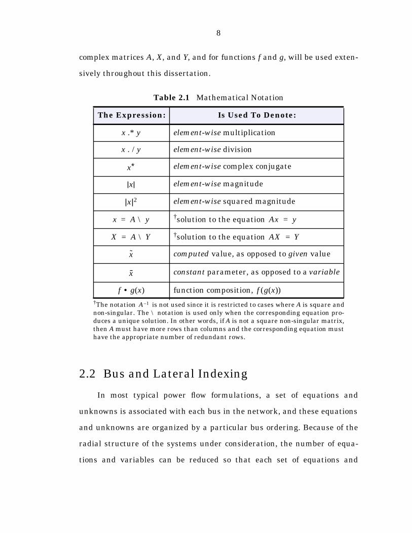
tions. The conventions shown in Table 2.1 for complex vectors x and y, for

8

complex matrices A, X, and Y, and for functions f and g, will be used exten-

sively throughout this dissertation.

2.2 Bus and Lateral Indexing

In most typical power flow formulations, a set of equations and

unknowns is associated with each bus in the network, and these equations

and unknowns are organized by a particular bus ordering. Because of the

radial structure of the systems under consideration, the number of equa-

tions and variables can be reduced so that each set of equations and

†The notation is not used since it is restricted to cases where A is square andnon-singular. The \ notation is used only when the corresponding equation pro-duces a unique solution. In other words, if A is not a square non-singular matrix,then A must have more rows than columns and the corresponding equation musthave the appropriate number of redundant rows.

Table 2.1 Mathematical Notation

The Expression: Is Used To Denote:

element-wise multiplication

element-wise division

element-wise complex conjugate

element-wise magnitude

element-wise squared magnitude

†solution to the equation

†solution to the equation

computed value, as opposed to given value

constant parameter, as opposed to a variable

function composition,

x y.*

x y. /

x∗

x

x 2

x A y\= Ax y=

A 1–

X A Y\= AX Y=

x

x

f g• x( ) f g x( )( )

9

unknowns corresponds to an entire lateral instead of an individual bus.

Such a formulation therefore calls for an appropriate lateral indexing to

order these equations and variables.

2.2.1 Indexing Scheme

A radial system can be thought of as a main feeder with laterals.

These laterals may also have sub-laterals, which themselves may have

sub-laterals, etc. First, the level of lateral i is defined as the number of lat-

erals which need to be traversed to go from the end of lateral i to the

source. For example, the main feeder would be level 1, its sub-laterals

would be level 2, their sub-laterals level 3, etc.

Second, the laterals within level l are indexed according to the order

seen during a breadth-first traversal of the network. Each lateral can be

uniquely identified by an ordered pair where l is the lateral level and

m is the lateral index within level l.

Third, buses are indexed within each lateral, starting with the first

bus on the lateral, so that each bus is uniquely identified by an ordered tri-

ple where n is the bus index. The ordered triple refers to

the nth bus on the mth level l lateral. The source is given an index of

. The number of levels in a network will be denoted by L, the num-

ber of laterals on level l by , and the number of buses on lateral

by .

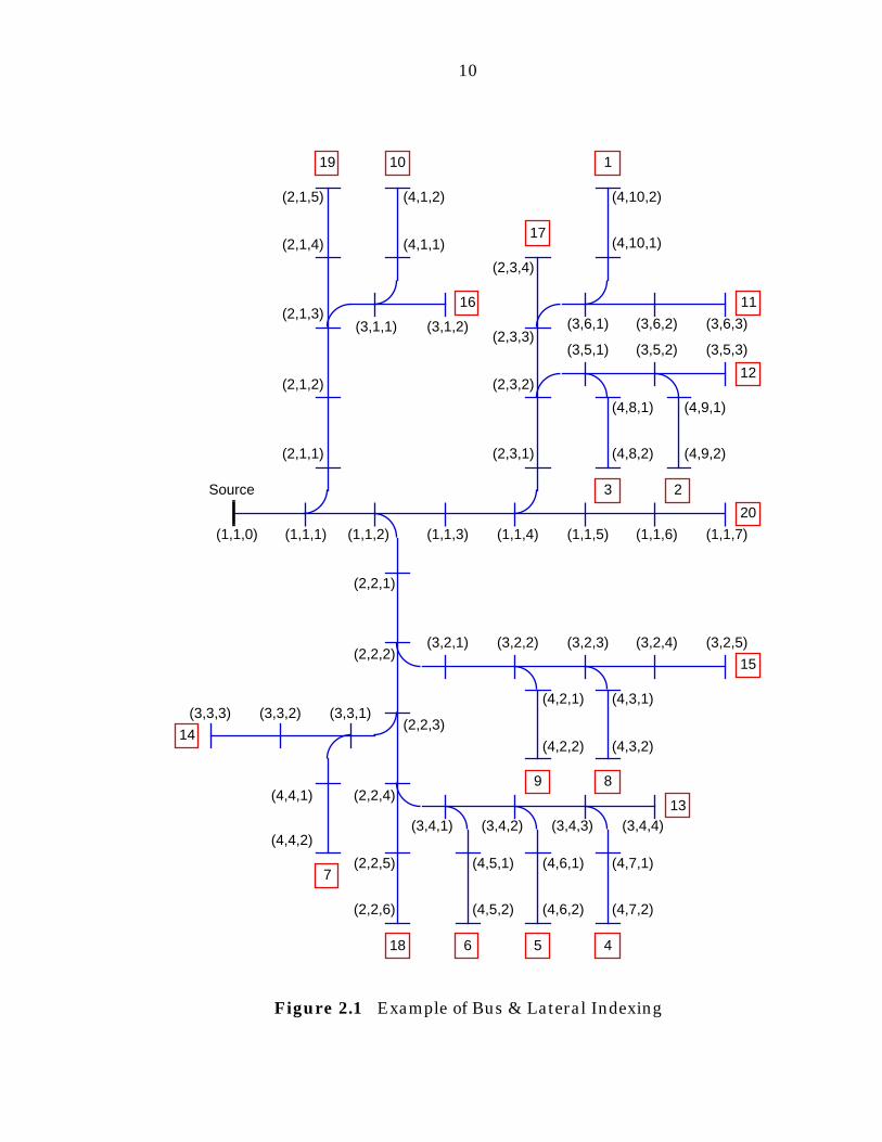
Figure 2.1 shows an example of this indexing scheme on a sample

63-bus system. The boxed numbers show the reverse breadth-first (RBF)

ordering of the laterals found by sorting the lateral indices in descending

order, first by level, then by lateral index. The RBF ordering is typically

l m,( )

l m n, ,( ) l m n, ,( )

1 1 0, ,( )

Ml l m,( )

N l m,

10

Figure 2.1 Example of Bus & Lateral Indexing

(1,1,0) (1,1,1) (1,1,2) (1,1,3) (1,1,4) (1,1,5) (1,1,6) (1,1,7)

(2,3,1)

(2,3,2)

(3,6,1)

(2,3,4)

(2,3,3)(3,6,2) (3,6,3)

(3,5,3)(3,5,2)(3,5,1)

(4,9,1)

(4,9,2)(2,1,1)

(2,1,2)

(2,1,3)

(2,1,4)

(2,1,5)

(3,1,1) (3,1,2)

Source

(4,1,2)

(4,1,1)

(2,2,4)

(2,2,3)

(2,2,1)

(2,2,2)

(2,2,5)

(2,2,6)

(4,4,2)

(4,4,1)

(3,3,3) (3,3,2) (3,3,1)

(3,2,1) (3,2,2) (3,2,3) (3,2,4) (3,2,5)

(4,3,1)

(4,3,2)(4,2,2)

(4,2,1)

(4,7,1)

(4,7,2)

(4,6,1)

(4,6,2)(4,5,2)

(4,5,1)

(3,4,1) (3,4,2) (3,4,3) (3,4,4)

(4,8,2)

(4,8,1)

(4,10,1)

(4,10,2)

1

3 2

456

8

7

9

10

11

13

12

15

16

18

17

19

20

14

11

used for backward sweep type operations. If the laterals are sorted in

ascending order, the result is a breadth-first (BF) ordering, typically used

for forward sweep type operations.

The following shorthand notation will also be used when i is an

ordered pair referring to a lateral and k is an ordered triple referring to a

bus. Lateral refers to the parent of lateral i, and bus refers to

bus k’s parent bus. Unless specified otherwise, bus is used to refer to

the bus following bus k on the same lateral. This is consistent with using k

as a simple bus index, in other words letting , which is done fre-

quently throughout the following chapters. In this case, bus 0 of lateral i

refers to the bus on lateral from which lateral i emanates. For exam-

ple, in the network in Figure 2.1, bus 0 of lateral (2,3) is also bus 4 of lat-

eral (1,1). This notation is used in indexing voltages, currents, power flows,

impedances, etc.

2.2.2 Indexing Implementation

All of the algorithms discussed in Chapters 4, 5, 6, and 7 use the

ordering of the buses and laterals presented in the previous section. They

also require the ability to traverse any given lateral from its source to its

end bus or vice versa. Certain data structures are therefore needed in the

program to store information about connectivity and ordering. Also

required is a process by which this information is generated from the origi-

nal network data.

2.2.2.1 Connectivity Data Structures

The network data which specifies the topology of the system is typi-

cally given as a list of branches with information on which two buses the

i 1– k 1–

k 1+

k n=

i 1–

12

branch connects. In order to efficiently traverse a feeder, it is important to

store information with each bus k indicating the incoming branch, the bus

which follows bus k on the same lateral, the number of sub-laterals

branching off at bus k, and the first bus on each of these sub-laterals.

The first three of these quantities will be denoted inbranch(k),

next(k), and nsubs(k), respectively. The first bus on the sub-laterals

branching from bus k will be called subbus1(k,1), subbus1(k,2), …,

subbus1(k,nsubs(k)), respectively. Assuming the source bus is known,

these data structures can be built up, along with the ordered triples of the

previous section, during the process of a breadth-first search.

2.2.2.2 Breadth-First Search

The initial traversal of the network is done via a breadth-first search

algorithm. This traversal can be useful for many things such as detecting

isolated sub-networks, checking the consistency of the phase data,1 and

marking sections of the network as grounded or ungrounded. However, the

primary purpose is to build up the connectivity data structures and assign

the bus and lateral indices. It should be noted that a depth-first search

works equally well for building the connectivity data structures and index-

ing the buses. The breadth-first approach was chosen for convenience in

dealing with weakly meshed networks as discussed in Chapter 7.

The breadth-first search, as described in [22], requires the ability to

find all of the “children” associated with a given node of the tree. Since the

connectivity structures are not yet available, the children of bus k must be

found via brute force by searching all branches for those connected to

1 How many and which phases are present at each bus and branch and do they match.

13

bus k. If the bus at the other end of such a branch has not yet been visited

during the search,2 it is a child of bus k.

When the search is at bus k and all of bus k’s children have been

found, the inbranch information can be set for each child. The value of

nsubs is typically set to one less than the number of children since one of

the children is generally selected to be the next bus on the same lateral

and the rest are assigned to the elements of subbus1.

The decision of which child, if any, is considered to be on the continua-

tion of the same lateral and which children are considered to be on sub-lat-

erals has a significant effect on the resulting bus and lateral indexing.

Since some of the power flow algorithms require that each lateral have at

most one transformer, a child whose inbranch is a transformer is never

assigned to next. Transformers are always assigned to a sub-lateral, even

if it leads to the bus’s only child. Similarly, if the branch leading to a child

of bus k has fewer phases than bus k, then the child is put on a sub-lateral.

This simplifies some of the implementation since it means that the phases

present are consistent throughout an entire lateral.

After setting the connectivity data structures at bus k, the bus’s

ordered triple is generated. This requires several counters to be main-

tained during the search process. First, l, m, and n are used to denote the

current level, lateral, and bus indices, respectively. The counters L, ,

and keep track of the number of levels encountered during the

search, the number of laterals on level l, and the number of buses on

lateral , respectively. The algorithm used to generate the ordered tri-

ple for bus k is shown in Table 2.2.

2 i.e. the branch is not the incoming branch of bus k (assuming a radial network).

Ml

N l m,

l m,( )

14

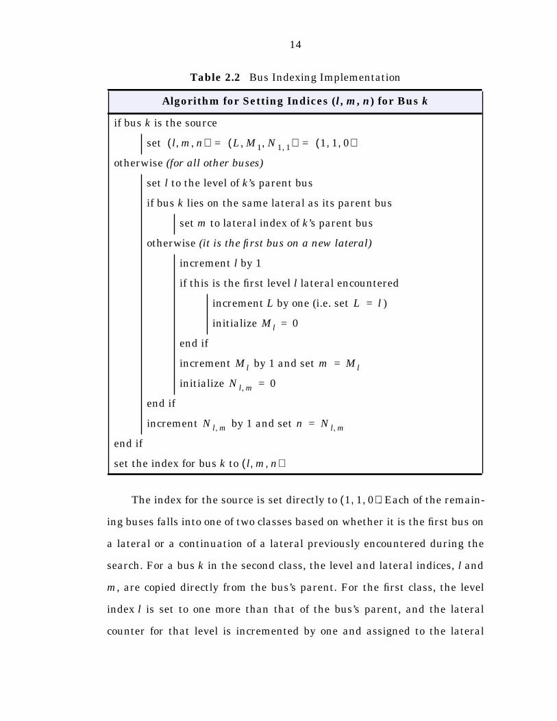
The index for the source is set directly to . Each of the remain-

ing buses falls into one of two classes based on whether it is the first bus on

a lateral or a continuation of a lateral previously encountered during the

search. For a bus k in the second class, the level and lateral indices, l and

m, are copied directly from the bus’s parent. For the first class, the level

index l is set to one more than that of the bus’s parent, and the lateral

counter for that level is incremented by one and assigned to the lateral

Table 2.2 Bus Indexing Implementation

Algorithm for Setting Indices (l, m, n) for Bus k

if bus k is the source

set

otherwise (for all other buses)

set l to the level of k’s parent bus

if bus k lies on the same lateral as its parent bus

set m to lateral index of k’s parent bus

otherwise (it is the first bus on a new lateral)

increment l by 1

if this is the first level l lateral encountered

increment L by one (i.e. set )

initialize

end if

increment by 1 and set

initialize

end if

increment by 1 and set

end if

set the index for bus k to

l m n, ,( ) L M1 N1 1,, ,( ) 1 1 0, ,( )= =

L l=

Ml 0=

Ml m Ml=

N l m, 0=

N l m, n N l m,=

l m n, ,( )

1 1 0, ,( )

15

index m. Finally, in both cases, the bus counter for that lateral is incre-

mented by one and assigned as the bus index n. Each time a new level l is

first encountered, L is incremented and assigned to l and the correspond-

ing lateral counter is initialized to zero. Likewise, each time a new

level l lateral is first encountered, is incremented and assigned to m

and the corresponding bus counter is initialized to zero.

When the entire network has been traversed by the search, all connec-

tivity structures have been built and all bus indices have been assigned.

These bus indices are then used to form a list of laterals in RBF3 order.

Each element of the list contains the first and last buses on the correspond-

ing lateral. These elements are sorted in descending order according to the

indices associated with the corresponding buses, first by the lateral level,

then by the lateral index.

2.3 Basic System Model

For the purposes of power flow studies, a radial distribution system

can be modeled as a network of buses connected by distribution lines,

switches, or transformers to a voltage specified source bus. Each bus may

also have a corresponding load, shunt capacitor, and/or cogenerator con-

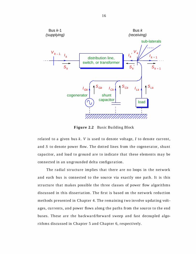
nected to it. The model can be represented by a radial interconnection of

copies of the basic building block shown in Figure 2.2. Since a given branch

may be single-phase, two-phase, or three-phase, each of the labeled quanti-

ties is, respectively, a complex scalar, a 2 x 1, or a 3 x 1 complex vector.

Figure 2.2 establishes a consistent notation, which will be used extensively

throughout this dissertation, for the voltages, currents, and power flows

3 See page 9 under Section 2.2.1, “Indexing Scheme”.

Ml

Ml

N l m,

16

related to a given bus k. V is used to denote voltage, I to denote current,

and S to denote power flow. The dotted lines from the cogenerator, shunt

capacitor, and load to ground are to indicate that these elements may be

connected in an ungrounded delta configuration.

The radial structure implies that there are no loops in the network

and each bus is connected to the source via exactly one path. It is this

structure that makes possible the three classes of power flow algorithms

discussed in this dissertation. The first is based on the network reduction

methods presented in Chapter 4. The remaining two involve updating volt-

ages, currents, and power flows along the paths from the source to the end

buses. These are the backward/forward sweep and fast decoupled algo-

rithms discussed in Chapter 5 and Chapter 6, respectively.

Figure 2.2 Basic Building Block

Bus k-1 Bus k

distribution line,

sub-laterals

V k 1– Ik

V kIk 1+

SLk

cogenerator shuntcapacitor

load

SCkSGk

(supplying) (receiving)

Ik′

switch, or transformerSk Sk

′ Sk 1+

ILkICkIGk

17

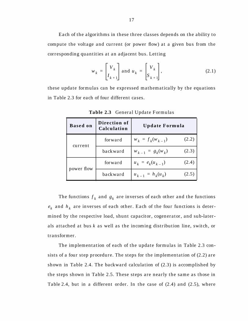
Each of the algorithms in these three classes depends on the ability to

compute the voltage and current (or power flow) at a given bus from the

corresponding quantities at an adjacent bus. Letting

and , (2.1)

these update formulas can be expressed mathematically by the equations

in Table 2.3 for each of four different cases.

The functions and are inverses of each other and the functions

and are inverses of each other. Each of the four functions is deter-

mined by the respective load, shunt capacitor, cogenerator, and sub-later-

als attached at bus k as well as the incoming distribution line, switch, or

transformer.

The implementation of each of the update formulas in Table 2.3 con-

sists of a four step procedure. The steps for the implementation of (2.2) are

shown in Table 2.4. The backward calculation of (2.3) is accomplished by

the steps shown in Table 2.5. These steps are nearly the same as those in

Table 2.4, but in a different order. In the case of (2.4) and (2.5), where

Table 2.3 General Update Formulas

Based onDirection ofCalculation

Update Formula

currentforward (2.2)

backward (2.3)

power flowforward (2.4)

backward (2.5)

wk

Vk

Ik 1+

= uk

Vk

Sk 1+

=

wk f k wk 1–( )=

wk 1– gk wk( )=

uk ek uk 1–( )=

uk 1– hk uk( )=

f k gk

ek hk

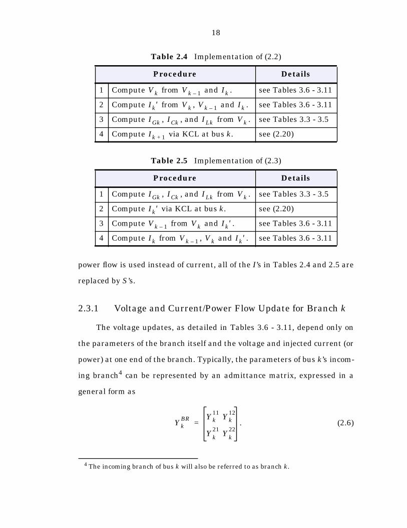
18

power flow is used instead of current, all of the I’s in Tables 2.4 and 2.5 are

replaced by S’s.

2.3.1 Voltage and Current/Power Flow Update for Branch k

The voltage updates, as detailed in Tables 3.6 - 3.11, depend only on

the parameters of the branch itself and the voltage and injected current (or

power) at one end of the branch. Typically, the parameters of bus k’s incom-

ing branch4 can be represented by an admittance matrix, expressed in a

general form as

. (2.6)

4 The incoming branch of bus k will also be referred to as branch k.

Table 2.4 Implementation of (2.2)

Procedure Details

1 Compute from and . see Tables 3.6 - 3.11

2 Compute from , and . see Tables 3.6 - 3.11

3 Compute , , and from . see Tables 3.3 - 3.5

4 Compute via KCL at bus k. see (2.20)


Procedure Details


2 Compute via KCL at bus k. see (2.20)



Vk Vk 1– Ik

Ik′ Vk Vk 1– Ik

IGk ICk ILk Vk

Ik 1+

IGk ICk ILk Vk

Ik′

Vk 1– Vk Ik′

Ik Vk 1– Vk Ik′

YkBR Yk

11Yk

12

Yk21

Yk22

=

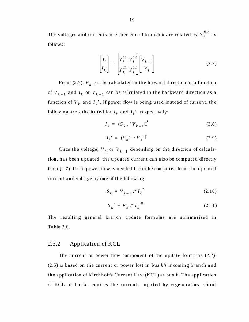
19

The voltages and currents at either end of branch k are related by as

follows:

(2.7)

From (2.7), can be calculated in the forward direction as a function

of and or can be calculated in the backward direction as a

function of and . If power flow is being used instead of current, the

following are substituted for and , respectively:

(2.8)

(2.9)

Once the voltage, or depending on the direction of calcula-

tion, has been updated, the updated current can also be computed directly

from (2.7). If the power flow is needed it can be computed from the updated

current and voltage by one of the following:

(2.10)

(2.11)

The resulting general branch update formulas are summarized in

Table 2.6.

2.3.2 Application of KCL

The current or power flow component of the update formulas (2.2)-

(2.5) is based on the current or power lost in bus k’s incoming branch and

the application of Kirchhoff’s Current Law (KCL) at bus k. The application

of KCL at bus k requires the currents injected by cogenerators, shunt

YkBR

Ik

Ik′

Yk11

Yk12

Yk21

Yk22

Vk 1–

Vk

=

Vk

Vk 1– Ik Vk 1–

Vk Ik′

Ik Ik′

Ik Sk Vk 1–. /( ) ∗=

Ik′ Sk′ Vk. /( ) ∗=

Vk

Vk 1–

Sk Vk 1– Ik∗.*=

Sk′ Vk Ik′∗.*=

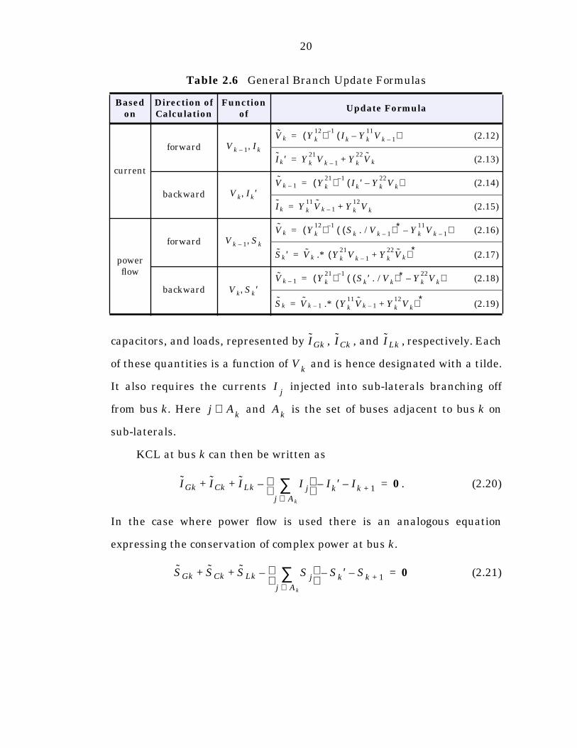
20

capacitors, and loads, represented by , , and , respectively. Each

of these quantities is a function of and is hence designated with a tilde.

It also requires the currents injected into sub-laterals branching off

from bus k. Here and is the set of buses adjacent to bus k on

sub-laterals.

KCL at bus k can then be written as

. (2.20)

In the case where power flow is used there is an analogous equation

expressing the conservation of complex power at bus k.

(2.21)

Table 2.6 General Branch Update Formulas

Based on

Direction ofCalculation

Functionof

Update Formula

current

forward(2.12)

(2.13)

backward(2.14)

(2.15)

power flow

forward(2.16)

(2.17)

backward(2.18)

(2.19)

Vk 1– Ik,Vk Yk

12( ) 1–Ik Yk

11Vk 1––( )=

Ik′ Yk21

Vk 1– Yk22

Vk+=

Vk Ik′,Vk 1– Yk

21( ) 1–Ik′ Yk

22Vk–( )=

Ik Yk11

Vk 1– Yk12

Vk+=

Vk 1– Sk,Vk Yk

12( ) 1–Sk Vk 1–. /( ) ∗ Yk

11Vk 1––( )=

Sk′ Vk Yk21

Vk 1– Yk22

Vk+( ) ∗.*=

Vk Sk′,Vk 1– Yk

21( ) 1–Sk′ Vk. /( ) ∗ Yk

22Vk–( )=

Sk Vk 1– Yk11

Vk 1– Yk12

Vk+( ) ∗.*=

IGk ICk ILk

Vk

Ij

j Ak

∈ Ak

IGk ICk ILk I jj Ak∈∑

– Ik′– Ik 1+–+ + 0=

SGk SCk SLk S jj Ak∈∑

– Sk′– Sk 1+–+ + 0=

21

Chapter 3

Detailed Component Models

In any problem where mathematics and numerical algorithms are

used to analyze a physical system, the results are only as accurate as the

mathematical models used. In power systems analysis, the solutions found

by any power flow algorithm are only useful to the user if they provide

results which are meaningful with respect to some real system. It is there-

fore important to model each component of the system as accurately as

possible. On the other hand, care must be taken to avoid using models

which are overly detailed and therefore either computationally impractical

or unusable due to unavailability of parameter data. The algorithms pre-

sented in this dissertation are based on models which attempt to meet

these two requirements. Most are based on standard three-phase models

as presented in [2; 8; 10].

This chapter describes in detail the models used for loads, shunt

capacitors, cogenerators, distribution lines, switches, and transformers.

These models provide relationships between the relevant voltages, cur-

rents, and power flows. By convention, injected currents and power flows

22

are always used for loads, shunt capacitors, and cogenerators, as shown in

Figure 2.2.

Bus voltages are typically the phase voltages , , and refer-

enced to ground. However, it is possible to have floating sections of the net-

work in which there is no reference to ground. For example, there might be

a feeder connected to the secondary side of a grounded wye to delta trans-

former which has only ungrounded, i.e. delta connected, loads. The terms

grounded and ungrounded, respectively, will be used to distinguish

between parts of the network which have a reference to ground and those

floating sections which do not. Which buses are in grounded sections and

which are in ungrounded sections is determined according to the ground-

ing of the transformer connections during the initial traversal of the net-

work described in Section 2.2.2.2, “Breadth-First Search”. It is assumed

that any part of a network supplied through an ungrounded transformer

connection will be entirely ungrounded.1

In the ungrounded sections, to avoid arbitrarily picking a particular

phase as the voltage reference, the line-to-line voltages and are

used. In this case, the third line voltage is redundant since it is always

equal to , and the dimension of the equations is reduced by

one. Similarly, the current in one of the phases is redundant since

, so typically only phase a and phase b currents are used

for calculation.

1 A sub-network, supplied through an ungrounded transformer connection, which doeshave some grounded elements could be handled by the network reduction methods ofChapter 4, though the details of such a case are not discussed. In their current forms,however, the methods of Chapter 5 and Chapter 6 are unable to handle this case.

Va

Vb

Vc

Vab

Vbc

Vca

Vab

Vbc

+( )–

Ic

Ia

Ib

+( )–=

23

When computing power flows as opposed to currents, ground is used

as a reference in grounded sections. For example, . However,

in ungrounded sections, the power used is that defined by the line-to-line

voltages and , and the currents and .

(3.1)

(3.2)

It is important to note that, although it is possible to calculate total power

flows in grounded sections of the network by the sum , the

total power flow in an ungrounded section is not equal to . Total

power flows must be calculated using a common voltage base. For example,

using phase c as a voltage reference, the total power can be computed as

. (3.3)

3.1 Load Model

The model used for loads is a flexible one. It includes constant com-

plex power, constant current, and constant impedance types.2 Three-phase

loads can be balanced or unbalanced and can be connected in a grounded

wye configuration or an ungrounded delta configuration. It is also possible

to have single-phase or two-phase grounded loads. Typically, the load val-

ues are given as nominal power delivered to the load and must be con-

verted into the appropriate constant model parameters. Depending on the

type of power flow algorithm being utilized, it may be necessary to compute

2 Each load could actually be a linear combination of these three types. In fact, it isstraightforward to generalize the model presented here to a current injection expressed asan arbitrary function of voltage.

Sa

VaI

a∗=

Vab

Vbc

Ia

Ib

Sab

Vab

Ia∗

=

Sbc

Vbc

Ib∗

=

Sa

Sb

Sc

+ +

Sab

Sbc

+

Stotal

Sac

Sbc

+=

24

the following quantities from the bus voltage and the constant model

parameters:

• admittance matrix

• injected current

• injected power

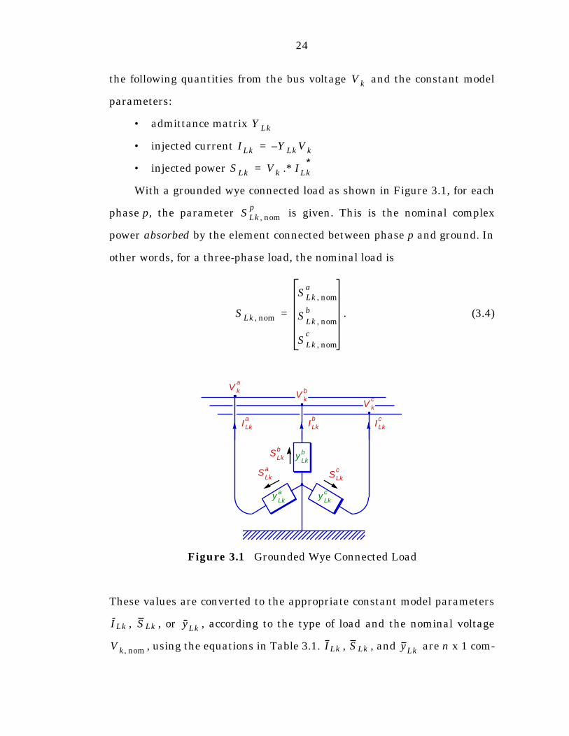
With a grounded wye connected load as shown in Figure 3.1, for each

phase p, the parameter is given. This is the nominal complex

power absorbed by the element connected between phase p and ground. In

other words, for a three-phase load, the nominal load is

. (3.4)

These values are converted to the appropriate constant model parameters

, , or , according to the type of load and the nominal voltage

, using the equations in Table 3.1. , , and are n x 1 com-

Figure 3.1 Grounded Wye Connected Load

Vk

Y Lk

ILk Y LkVk–=

SLk Vk ILk∗.*=

SLk nom,p

SLk nom,

SLk nom,a

SLk nom,b

SLk nom,c

=

yLk

b

yLk

a yLk

c

V k

c

ILk

a

SLk

b

SLk

cSLk

a

ILk

bILk

c

V k

a

Vk

b

ILk SLk yLk

Vk nom, ILk SLk yLk

25

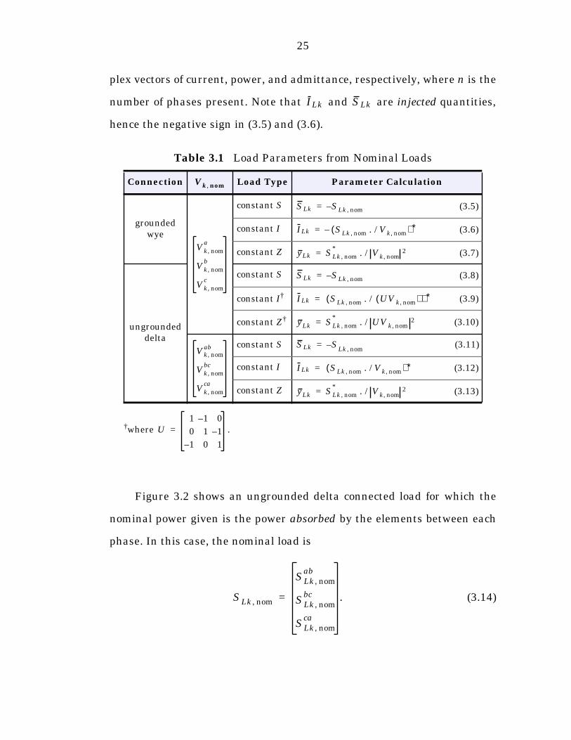
plex vectors of current, power, and admittance, respectively, where n is the

number of phases present. Note that and are injected quantities,

hence the negative sign in (3.5) and (3.6).

Figure 3.2 shows an ungrounded delta connected load for which the

nominal power given is the power absorbed by the elements between each

phase. In this case, the nominal load is

. (3.14)

†where .

Table 3.1 Load Parameters from Nominal Loads

Connection Load Type Parameter Calculation

grounded wye

constant S (3.5)

constant I (3.6)

constant Z (3.7)

ungrounded delta

constant S (3.8)

constant I† (3.9)

constant Z† (3.10)

constant S (3.11)

constant I (3.12)

constant Z (3.13)

ILk SLk

Vk nom,

Vk nom,a

Vk nom,b

Vk nom,c

SLk SLk nom,–=

ILk SLk nom, Vk nom,. /( ) ∗–=

yLk SLk nom,*

Vk nom,2. /=

SLk SLk nom,–=

U1 1– 0

0 1 1–

1– 0 1

=

ILk SLk nom, UV k nom,( ). /( ) ∗=

yLk SLk nom,*

UV k nom,2. /=

Vk nom,ab

Vk nom,bc

Vk nom,ca

SLk SLk nom,–=

ILk SLk nom, Vk nom,. /( ) ∗=

yLk SLk nom,*

Vk nom,2. /=

SLk nom,

SLk nom,ab

SLk nom,bc

SLk nom,ca

=

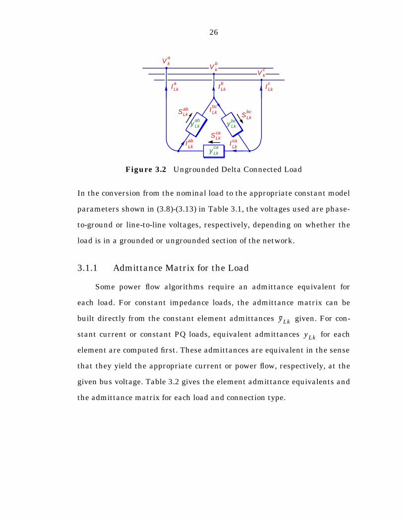
26

In the conversion from the nominal load to the appropriate constant model

parameters shown in (3.8)-(3.13) in Table 3.1, the voltages used are phase-

to-ground or line-to-line voltages, respectively, depending on whether the

load is in a grounded or ungrounded section of the network.

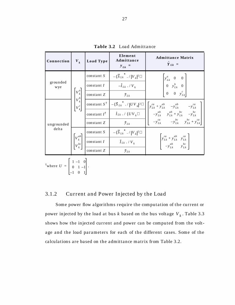
3.1.1 Admittance Matrix for the Load

Some power flow algorithms require an admittance equivalent for

each load. For constant impedance loads, the admittance matrix can be

built directly from the constant element admittances given. For con-

stant current or constant PQ loads, equivalent admittances for each

element are computed first. These admittances are equivalent in the sense

that they yield the appropriate current or power flow, respectively, at the

given bus voltage. Table 3.2 gives the element admittance equivalents and

the admittance matrix for each load and connection type.

Figure 3.2 Ungrounded Delta Connected Load

V k

c

ILk

aILk

bILk

c

V k

a

V k

b

y Lkbcy Lk

ab

y Lk

ca

SLk

bc

SLkca

SLkab

ILk

ab

ILk

bc

ILk

ca

yLk

yLk

27

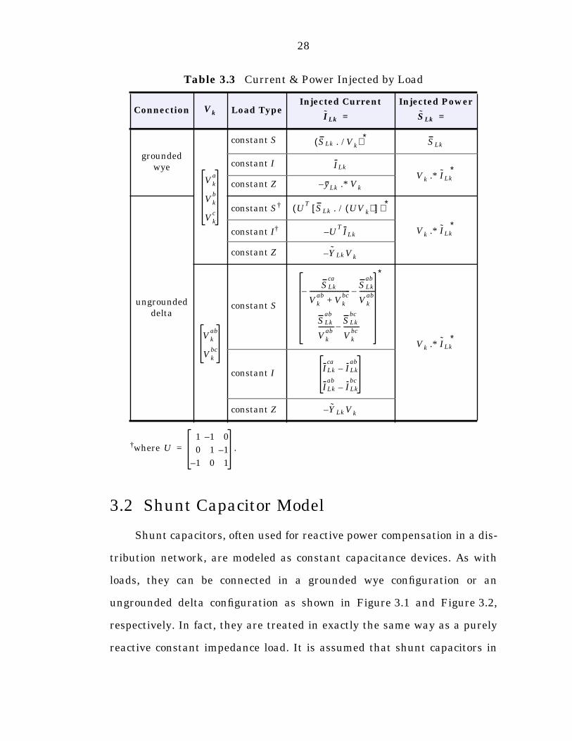
3.1.2 Current and Power Injected by the Load

Some power flow algorithms require the computation of the current or

power injected by the load at bus k based on the bus voltage . Table 3.3

shows how the injected current and power can be computed from the volt-

age and the load parameters for each of the different cases. Some of the

calculations are based on the admittance matrix from Table 3.2.

†where .

Table 3.2 Load Admittance

Connection Load TypeElement

AdmittanceAdmittance Matrix

grounded wye

constant S

constant I

constant Z

ungrounded delta

constant S†

constant I†

constant Z

constant S

constant I

constant Z

Vk

yLk

= Y Lk =

Vka

Vkb

Vkc

SLk∗ Vk

2. /( )– yLka 0 0

0 yLkb 0

0 0 yLkc

ILk Vk. /–

yLk

U1 1– 0

0 1 1–

1– 0 1

=

SLk∗ UV

k2. /( )– yLk

cayLk

ab+ y– Lk

aby– Lk

ca

y– Lkab

yLkab

yLkbc

+ y– Lkbc

y– Lkca

y– Lkbc

yLkbc

yLkca

+

ILk UV k( ). /

yLk

Vkab

Vkbc

SLk∗ Vk

2. /( )–

yLkca

yLkab

+ yLkca

yLkab

– yLkbc

ILk Vk. /

yLk

Vk

28

3.2 Shunt Capacitor Model

Shunt capacitors, often used for reactive power compensation in a dis-

tribution network, are modeled as constant capacitance devices. As with

loads, they can be connected in a grounded wye configuration or an

ungrounded delta configuration as shown in Figure 3.1 and Figure 3.2,

respectively. In fact, they are treated in exactly the same way as a purely

reactive constant impedance load. It is assumed that shunt capacitors in

†where .

Table 3.3 Current & Power Injected by Load

Connection Load TypeInjected Current Injected Power

grounded wye

constant S

constant I

constant Z

ungrounded delta

constant S†

constant I†

constant Z

constant S

constant I

constant Z

Vk ILk = SLk =

Vka

Vkb

Vkc

SLk Vk. /( ) ∗ SLk

ILk

Vk ILk∗

.*yLk Vk.*–

UT

SLk UV k( ). /[ ]( ) ∗

Vk ILk∗

.*UT

ILk–

Y LkVk–

Vkab

Vkbc

SLkca

Vkab

Vkbc

+-------------------------–

SLkab

Vkab

---------–

SLkab

Vkab

---------SLk

bc

Vkbc

---------–

∗

Vk ILk∗

.*

ILkca

ILkab

–

ILkab

ILkbc

–

Y LkVk–

U1 1– 0

0 1 1–

1– 0 1

=

29

grounded sections of the network are wye connected and those in

ungrounded sections are three-phase and delta connected.

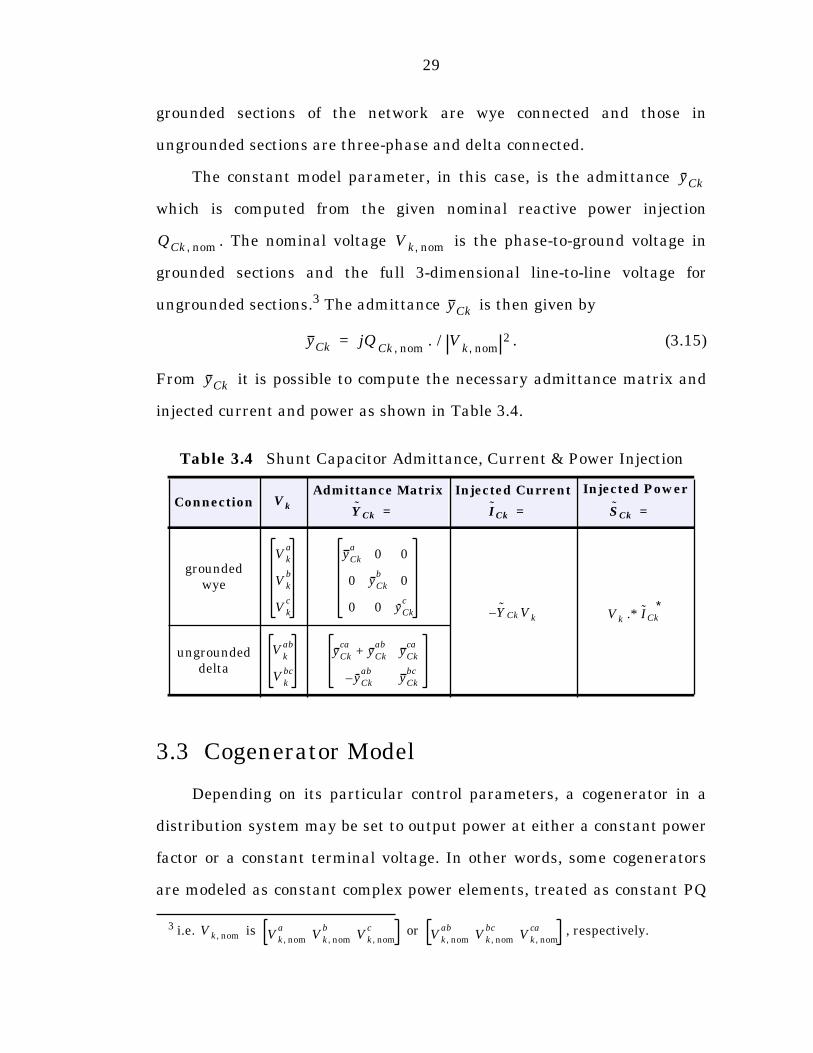
The constant model parameter, in this case, is the admittance

which is computed from the given nominal reactive power injection

. The nominal voltage is the phase-to-ground voltage in

grounded sections and the full 3-dimensional line-to-line voltage for

ungrounded sections.3 The admittance is then given by

. (3.15)

From it is possible to compute the necessary admittance matrix and

injected current and power as shown in Table 3.4.

3.3 Cogenerator Model

Depending on its particular control parameters, a cogenerator in a

distribution system may be set to output power at either a constant power

factor or a constant terminal voltage. In other words, some cogenerators

are modeled as constant complex power elements, treated as constant PQ

3 i.e. is or , respectively.

Table 3.4 Shunt Capacitor Admittance, Current & Power Injection

ConnectionAdmittance Matrix Injected Current Injected Power

grounded wye

ungrounded delta

yCk

QCk nom, Vk nom,

yCk

Vk nom, Vk nom,a

Vk nom,b

Vk nom,c

Vk nom,ab

Vk nom,bc

Vk nom,ca

yCk jQCk nom, V

k nom,2. /=

yCk

Vk YCk = ICk = SCk =

Vka

Vkb

Vkc

yCka

0 0

0 yCkb

0

0 0 yCkc

YCkVk– Vk ICk∗

.*

Vkab

Vkbc

yCkca

yCkab

+ yCkca

yCkab

– yCkbc

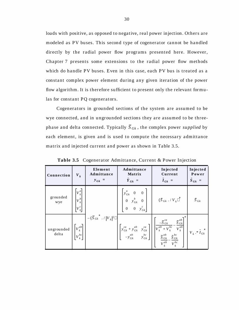
30

loads with positive, as opposed to negative, real power injection. Others are

modeled as PV buses. This second type of cogenerator cannot be handled

directly by the radial power flow programs presented here. However,

Chapter 7 presents some extensions to the radial power flow methods

which do handle PV buses. Even in this case, each PV bus is treated as a

constant complex power element during any given iteration of the power

flow algorithm. It is therefore sufficient to present only the relevant formu-

las for constant PQ cogenerators.

Cogenerators in grounded sections of the system are assumed to be

wye connected, and in ungrounded sections they are assumed to be three-

phase and delta connected. Typically , the complex power supplied by

each element, is given and is used to compute the necessary admittance

matrix and injected current and power as shown in Table 3.5.

Table 3.5 Cogenerator Admittance, Current & Power Injection

Connection

ElementAdmittance

AdmittanceMatrix

InjectedCurrent

InjectedPower

grounded wye

ungrounded delta

SGk

VkyGk = YGk = IGk = SGk =

Vka

Vkb

Vkc

SGk∗ Vk

2. /( )–

yGka

0 0

0 yGkb

0

0 0 yGkc

SGk Vk. /( ) ∗ SGk

Vkab

Vkbc

yGkca

yGkab

+ yGkca

yGkab

– yGkbc

S– Gkca

Vkab

Vkbc

+-------------------------

SGkab

Vkab

----------–

SGkab

Vkab

----------SGk

bc

Vkbc

----------–

∗

Vk IGk∗

.*

31

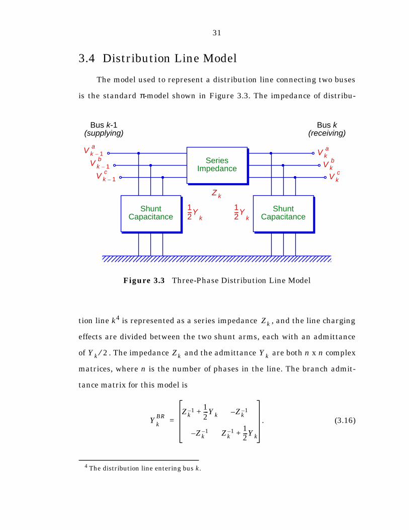
3.4 Distribution Line Model

The model used to represent a distribution line connecting two buses

is the standard π-model shown in Figure 3.3. The impedance of distribu-

tion line k4 is represented as a series impedance , and the line charging

effects are divided between the two shunt arms, each with an admittance

of . The impedance and the admittance are both n x n complex

matrices, where n is the number of phases in the line. The branch admit-

tance matrix for this model is

. (3.16)

4 The distribution line entering bus k.

Figure 3.3 Three-Phase Distribution Line Model

V kb

V kc

SeriesImpedance

ShuntCapacitance

V k 1–a

V k 1–b

V k 1–c

V ka

ShuntCapacitance

Bus k-1 Bus k(supplying) (receiving)

12---Y

k

Z k

12---Y

k

Zk

Yk 2⁄ Zk Yk

YkBR

Zk1– 1

2---Yk+ Zk

1––

Zk1–– Zk

1– 12---Yk+

=

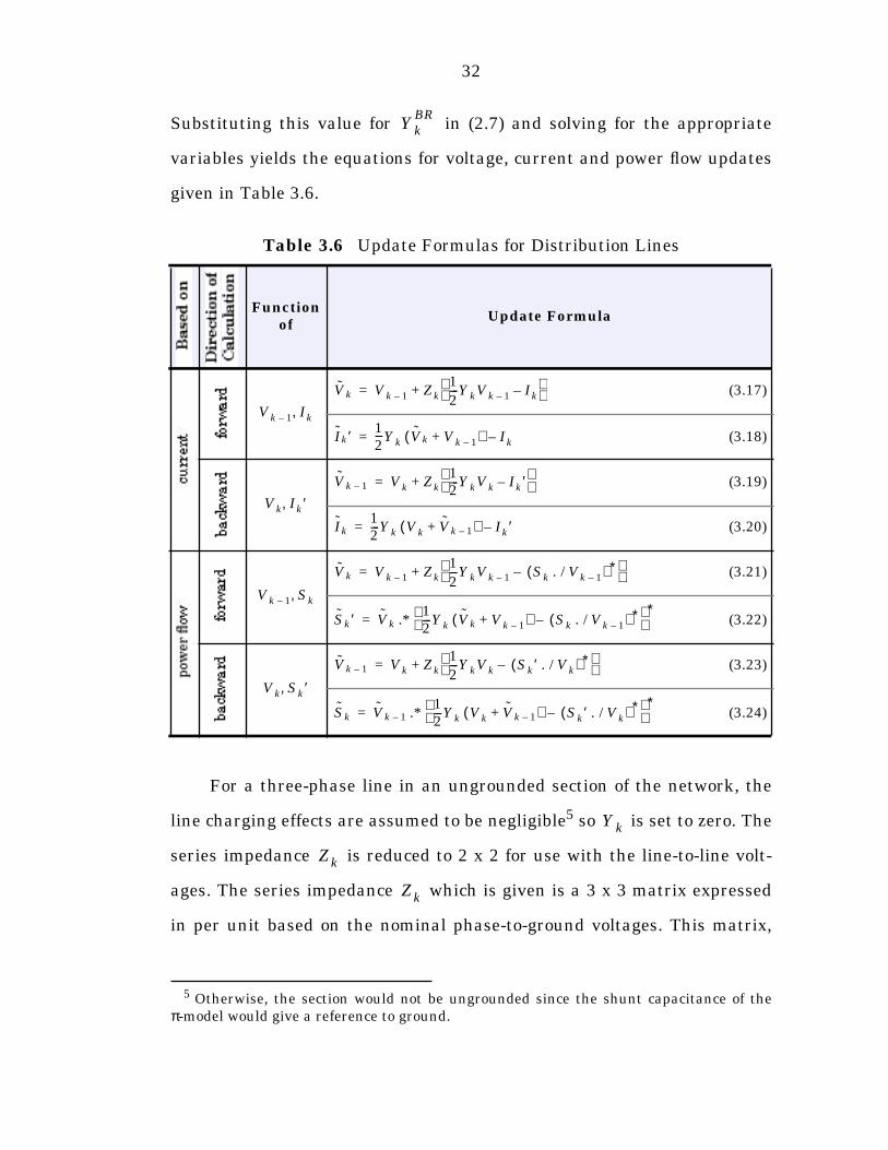
32

Substituting this value for in (2.7) and solving for the appropriate

variables yields the equations for voltage, current and power flow updates

given in Table 3.6.

For a three-phase line in an ungrounded section of the network, the

line charging effects are assumed to be negligible5 so is set to zero. The

series impedance is reduced to 2 x 2 for use with the line-to-line volt-

ages. The series impedance which is given is a 3 x 3 matrix expressed

in per unit based on the nominal phase-to-ground voltages. This matrix,

5 Otherwise, the section would not be ungrounded since the shunt capacitance of theπ-model would give a reference to ground.

Table 3.6 Update Formulas for Distribution Lines

Functionof

Update Formula

(3.17)

(3.18)

(3.19)

(3.20)

(3.21)

(3.22)

(3.23)

(3.24)

YkBR

Vk 1– Ik,Vk Vk 1– Zk

12---YkVk 1– Ik–

+=

Ik′ 12---Yk Vk Vk 1–+( ) Ik–=

Vk Ik′,Vk 1– Vk Zk

12---YkVk Ik′–

+=

Ik12---Yk Vk Vk 1–+( ) Ik′–=

Vk 1– Sk,Vk Vk 1– Zk

12---YkVk 1– Sk Vk 1–. /( ) ∗–

+=

Sk′ Vk12---Yk Vk Vk 1–+( ) Sk Vk 1–. /( ) ∗–

∗.*=

Vk Sk′,Vk 1– Vk Zk

12---YkVk Sk′ Vk. /( ) ∗–

+=

Sk Vk 1–12---Yk Vk Vk 1–+( ) Sk′ Vk. /( ) ∗–

∗.*=

Yk

Zk

Zk

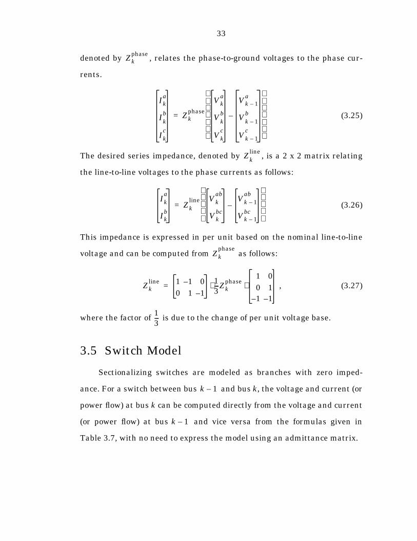
33

denoted by , relates the phase-to-ground voltages to the phase cur-

rents.

(3.25)

The desired series impedance, denoted by , is a 2 x 2 matrix relating

the line-to-line voltages to the phase currents as follows:

(3.26)

This impedance is expressed in per unit based on the nominal line-to-line

voltage and can be computed from as follows:

, (3.27)

where the factor of is due to the change of per unit voltage base.

3.5 Switch Model

Sectionalizing switches are modeled as branches with zero imped-

ance. For a switch between bus and bus k, the voltage and current (or

power flow) at bus k can be computed directly from the voltage and current

(or power flow) at bus and vice versa from the formulas given in

Table 3.7, with no need to express the model using an admittance matrix.

Zkphase

Ika

Ikb

Ikc

Zkphase

Vka

Vkb

Vkc

Vk 1–a

Vk 1–b

Vk 1–c

–

=

Zkline

Ika

Ikb

Zkline Vk

ab

Vkbc

Vk 1–ab

Vk 1–bc

–

=

Zkphase

Zkline 1 1– 0

0 1 1–

13---Zk

phase1 0

0 11– 1–

⋅ ⋅=

13---

k 1–

k 1–

34

3.6 Transformer Model

Three-phase transformers are modeled by an admittance matrix

which depends upon the connection type, the primary and secondary side

taps, and the leakage admittance. This admittance matrix for

transformer k6 is

. (3.36)

For a grounded wye to grounded wye transformer, this is a 6 x 6 complex

matrix relating primary and secondary side currents and primary and sec-

ondary side phase-to-ground voltages. In the case where one side of the

6 The transformer entering bus k.

Table 3.7 Update Formulas for Switches

Functionof

Update Formula

(3.28)

(3.29)

(3.30)

(3.31)

(3.32)

(3.33)

(3.34)

(3.35)

Vk 1– Ik,Vk Vk 1–=

Ik′ Ik–=

Vk Ik′,Vk 1– Vk=

Ik Ik′–=

Vk 1– Sk,Vk Vk 1–=

Sk′ Sk–=

Vk Sk′,Vk 1– Vk=

Sk Sk′–=

YkBR Y

kpp

Ykps

Yksp

Ykss

=

35

transformer is ungrounded, such as a delta or ungrounded wye connection,

line-to-line voltages are used and the dimension of the admittance matrix

is reduced to 5 x 5. If both sides are ungrounded, line-to-line voltages are

used on both sides and the dimension of is 4 x 4.

In the following sections, the primary side taps for transformer k are

denoted by , the secondary side taps by , and the per unit leakage

admittance per phase by . The admittance matrices for common trans-

former connections are given in Table 3.8. To simplify the presentation of

the relevant update formulas, the various transformer types are divided

into three classes based on the grounding of their connections.

3.6.1 Class A: Primary and Secondary both Grounded or both Ungrounded

The simplest class of transformer connections will be presented first.

This is the class of transformers which are either grounded on both sides or

ungrounded on both sides. This includes connection types 1, 5, 6, 8, and 9.

In this case, each submatrix of is square and non-singular so (3.36)

can be substituted into (2.7) to solve directly for the appropriate variables.

The resulting update formulas are given in Table 3.9.

3.6.2 Class B: Grounded Primary—Ungrounded Secondary

The second class of transformer connections to be presented is the

class of transformers with grounded primary side and ungrounded second-

ary side. This includes connection types 2 and 3. For these transformers,

the voltage, current, and power flow on the primary side are three-dimen-

sional quantities, but on the secondary side they are two-dimensional

quantities. There is a constraint, however, on the primary side currents

YkBR

αk βk

yk

YkBR

36

†i.e. swap and with and , respectively, then swap with .

Table 3.8 Admittance Matrices for Common Transformer Connections

Transformer Connection Type

Primary Secondary

1 A Grounded Wye Grounded Wye

2 B Grounded Wye Ungrounded Wye

3 B Grounded Wye Delta

4 C Ungrounded Wye Grounded Wye opposite† of type 2

5 A Ungrounded Wye Ungrounded Wye

6 A Ungrounded Wye Delta

7 C Delta Grounded Wye opposite† of type 3

8 A Delta Ungrounded Wye opposite† of type 6

9 A Delta Delta same as type 5

Ykpp

Ykps

Yksp

Ykss

yk

αk2

------1 0 0

0 1 0

0 0 1

yk–

αkβk

------------1 0 0

0 1 0

0 0 1

yk–

αkβk

------------1 0 0

0 1 0

0 0 1

yk

βk2

------1 0 0

0 1 0

0 0 1

yk

3αk2

----------2 1– 1–

1– 2 1–

1– 1– 2

yk–

3αkβk

--------------------2 1

1– 1

1– 2–

yk–

3αkβk

-------------------- 2 1– 1–

1– 2 1–

yk

βk2

------ 2 1

1– 1

yk

αk2

------1 0 0

0 1 0

0 0 1

yk–

αkβk

------------1 0

0 1

1– 1–

yk–

αkβk

------------ 1 0 1–

1– 1 0

yk

βk2

------ 2 1

1– 1

yk

αk2

------ 2 1

1– 1

yk–

αkβk

------------ 2 1

1– 1

yk–

αkβk

------------ 2 1

1– 1

yk

βk2

------ 2 1

1– 1

yk

αk2

------ 2 1

1– 1

3yk–

αkβk

----------------- 1 0

0 1

3yk–

αkβk

----------------- 1 1

1– 0

yk

βk2

------ 2 1

1– 1

Ykpp

Ykps

Ykss

Yksp αk βk

37

which effectively restricts it to two degrees of freedom. This constraint can

be expressed in terms of the sum of the currents on the primary side,

denoted by . For the type 2 grounded wye to ungrounded

wye case, the primary currents must sum to zero.

(3.45)

For type 3 grounded wye to delta connections, the sum of the primary cur-

rents is related to the sum of the primary voltages as follows:

, (3.46)

where .

In attempting to solve for the secondary voltage , (2.7) yields

, (3.47)

Table 3.9 Update Formulas for Class A Transformers

Functionof

Update Formula

(3.37)

(3.38)

(3.39)

(3.40)

(3.41)

(3.42)

(3.43)

(3.44)

Vk 1– Ik,Vk Yk

ps( ) 1–Ik Yk

ppVk 1––( )=

Ik′ Yksp

Vk 1– Ykss

Vk+=

Vk Ik′,Vk 1– Yk

sp( ) 1–Ik′ Yk

ssVk–( )=

Ik Ykpp Vk 1– Y

kpsV

k+=

Vk 1– Sk,Vk Yk

ps( ) 1–Sk Vk 1–. /( ) ∗ Yk

ppVk 1––( )=

Sk′ Vk YkspVk 1– Yk

ss Vk+( ) ∗.*=

Vk Sk′,Vk 1– Yk

sp( ) 1–Sk′ Vk. /( ) ∗ Yk

ssVk–( )=

Sk Vk 1– Ykpp

Vk 1– Ykps

Vk+( ) ∗.*=

IkΣ

Ika

Ikb

Ikc

+ +=

IkΣ

0=

IkΣ yk

αk2

------Vk 1–Σ

=

Vk 1–Σ

Vk 1–a

Vk 1–b

Vk 1–c

+ +=

Vk

Ykps

Vk

Ik

Ykpp

Vk 1––=

38

where is 3 x 2. This equation has a unique solution for only if

satisfies the appropriate constraint above, in which case one of the three

rows of (3.47) becomes redundant. Using the notation from Table 2.1, the

solution to this equation can be written as in (3.50) in Table 3.10.

Consider trying to solve for the primary side voltage from the lower

half of (2.7).

(3.48)

In this case, is 2 x 3 and, consequently, the secondary voltage and cur-

rent do not uniquely specify the primary voltage. It is only possible to solve

for if it is assumed that some information is already given, such as

the sum of the primary side voltages . If this information is given, the

solution to (3.48) can be written as in (3.52). In this case, used in (2.3)

must include .

(3.49)

So, for forward calculation, there is a constraint on the sum of the pri-

mary side currents. For backward calculation, information about the sum

of the primary side voltages must be available. Assuming these conditions

are met, the expressions for the updates can be written as shown in

Table 3.10.

Ykps

Vk IkΣ

Yksp

Vk 1– Ik′ Ykss

Vk–=

Yksp

Vk 1–

Vk 1–Σ

wk

Vk 1–Σ

wk

Vk

Vk 1–Σ

Ik 1+

=

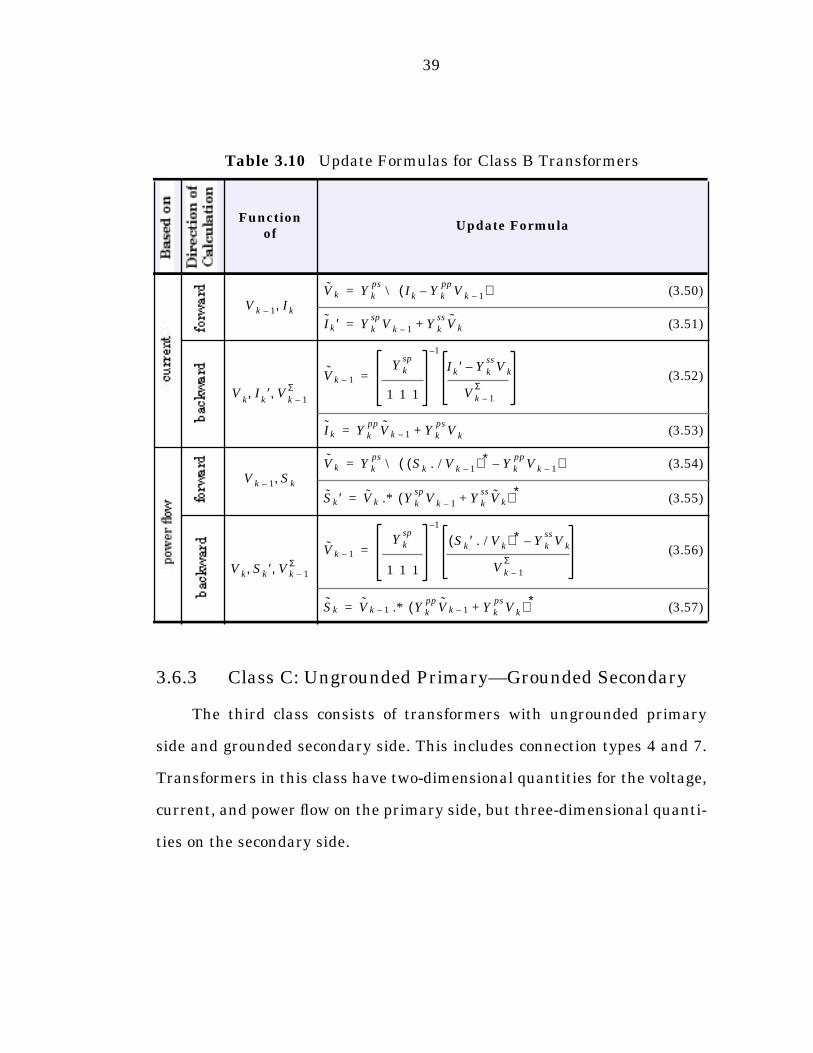
39

3.6.3 Class C: Ungrounded Primary—Grounded Secondary

The third class consists of transformers with ungrounded primary

side and grounded secondary side. This includes connection types 4 and 7.

Transformers in this class have two-dimensional quantities for the voltage,

current, and power flow on the primary side, but three-dimensional quanti-

ties on the secondary side.

Table 3.10 Update Formulas for Class B Transformers

Functionof

Update Formula

(3.50)

(3.51)

(3.52)

(3.53)

(3.54)

(3.55)

(3.56)

(3.57)

Vk 1– Ik,Vk Yk

psIk Yk

ppVk 1––( )\=

Ik′ Yksp

Vk 1– Ykss

Vk+=

Vk

Ik′ V

k 1–Σ, ,

Vk 1–

Yksp

1 1 1

1–

Ik′ Ykss

Vk–

Vk 1–Σ

=

Ik Ykpp

Vk 1– Ykps

Vk+=

Vk 1– Sk,Vk Yk

psSk Vk 1–. /( ) ∗ Yk

ppVk 1––( )\=

Sk′ Vk Yksp

Vk 1– Ykss

Vk+( ) ∗.*=

Vk Sk′ Vk 1–Σ, ,

Vk 1–

Yksp

1 1 1

1–

Sk′ Vk. /( ) ∗ Ykss

Vk–

Vk 1–Σ

=

Sk Vk 1– Ykpp

Vk 1– Ykps

Vk+( ) ∗.*=

40

In this case, the constraint on the sum of the currents is on the sec-

ondary side, i.e. on , and thus affects the backward cal-

culation. For the type 4 ungrounded wye to grounded wye case,

. (3.58)

For type 7 delta to grounded wye connections, the constraint on the current

is related to the sum of the secondary voltages .

(3.59)

Since is 3 x 2, the appropriate constraint above must be satisfied in

order to solve (3.48) for the primary voltage . The solution can be

expressed as in (3.63) in Table 3.11.

Forward calculation with transformers of class C is similar to back-

ward calculation with class B transformers. In this case, is 2 x 3 and

more information is needed to solve for a unique secondary voltage

from the primary voltage and current. If the sum of the secondary voltage

is known, that is sufficient to specify the secondary voltage completely.

However, in the power flow algorithms proposed in this dissertation, it is

actually current information, rather than voltage information, which is

available at the secondary side. For type 7 delta to grounded wye trans-

formers, (3.59) can be used to solve for from the sum of the secondary

current , allowing to be expressed as in (3.61). Here of (2.2)

must include .

(3.60)

IkΣ′ Ik

a′ Ikb′ Ik

c ′+ +=

IkΣ′ 0=

VkΣ

Vka

Vkb

Vkc

+ +=

IkΣ′

yk

βk2

------VkΣ

=

Yksp

Vk 1–

Ykps

Vk

VkΣ

VkΣ

IkΣ′ V

kw

k 1–

IkΣ′

wk 1–

Vk 1–

Ik

IkΣ′

=

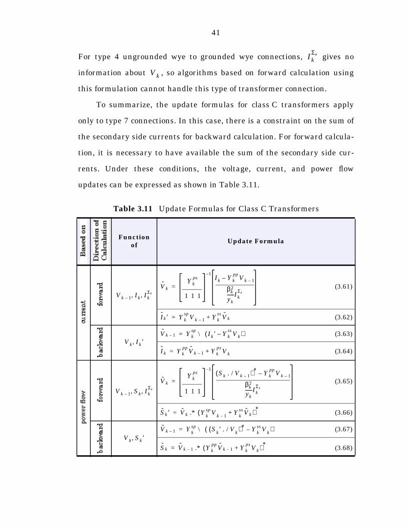
41

For type 4 ungrounded wye to grounded wye connections, gives no

information about , so algorithms based on forward calculation using

this formulation cannot handle this type of transformer connection.

To summarize, the update formulas for class C transformers apply

only to type 7 connections. In this case, there is a constraint on the sum of

the secondary side currents for backward calculation. For forward calcula-

tion, it is necessary to have available the sum of the secondary side cur-

rents. Under these conditions, the voltage, current, and power flow

updates can be expressed as shown in Table 3.11.

Table 3.11 Update Formulas for Class C Transformers

Functionof

Update Formula

(3.61)

(3.62)

(3.63)

(3.64)

(3.65)

(3.66)

(3.67)

(3.68)

IkΣ′

Vk

Vk 1– Ik IkΣ′, ,

Vk

Ykps

1 1 1

1–Ik Yk

ppVk 1––

βk2

yk

------IkΣ′

=

Ik′ Yksp

Vk 1– Ykss

Vk+=

Vk Ik′,Vk 1– Yk

spIk′ Yk

ssVk–( )\=

Ik Ykpp

Vk 1– Ykps

Vk+=

Vk 1– Sk IkΣ′, ,

Vk

Ykps

1 1 1

1–Sk Vk 1–. /( ) ∗ Yk

ppVk 1––

βk2

yk------Ik

Σ′=

Sk′ Vk YkspV

k 1–Y

kss Vk+( ) ∗.*=

Vk Sk′,Vk 1– Y

ksp S

k′ V

k. /( ) ∗ Y

kssV

k–( )\=

Sk Vk 1– Ykpp

Vk 1– Ykps

Vk+( ) ∗.*=

42

Chapter 4

Network Reduction Power Flow Algorithms for Radial Systems (NR-PARS)

The solution to the power flow problem is typically viewed as the solu-

tion to a set of power balance equations. It is possible, however, to look at

the problem from a circuit theory point of view. The distribution system, in

this context, is a circuit with one compound (three-phase) voltage source,

many constant impedance elements, and possibly some constant current

elements and some elements with a non-linear relationship between volt-

age and current (the constant power elements).

If each non-linear element is replaced by a linear element which is

equivalent in some sense, the new system can be solved using the standard

methods of nodal or loop analysis for linear circuits. Recomputing the lin-

ear equivalents at the new solution and repeating yields a basic iterative

method for solving the distribution power flow problem. In fact, this is

exactly the idea behind some of the Z-matrix methods in [9; 10; 25; 27].

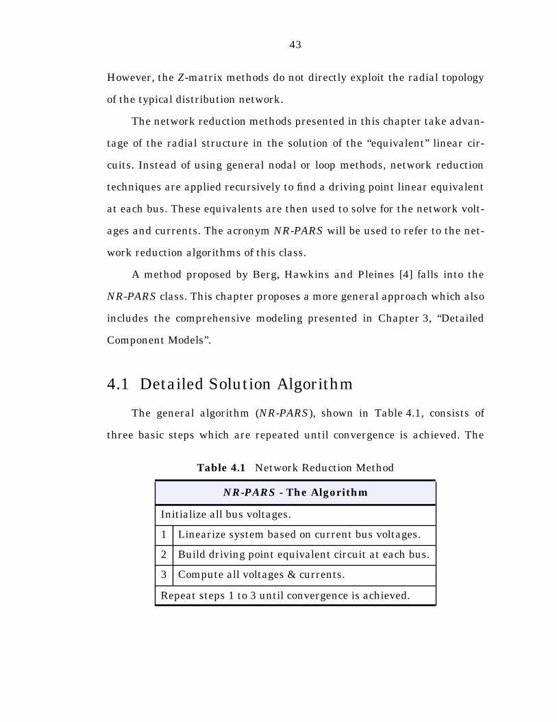
43

However, the Z-matrix methods do not directly exploit the radial topology

of the typical distribution network.

The network reduction methods presented in this chapter take advan-

tage of the radial structure in the solution of the “equivalent” linear cir-

cuits. Instead of using general nodal or loop methods, network reduction

techniques are applied recursively to find a driving point linear equivalent

at each bus. These equivalents are then used to solve for the network volt-

ages and currents. The acronym NR-PARS will be used to refer to the net-

work reduction algorithms of this class.

A method proposed by Berg, Hawkins and Pleines [4] falls into the

NR-PARS class. This chapter proposes a more general approach which also

includes the comprehensive modeling presented in Chapter 3, “Detailed

Component Models”.

4.1 Detailed Solution Algorithm

The general algorithm (NR-PARS), shown in Table 4.1, consists of

three basic steps which are repeated until convergence is achieved. The

Table 4.1 Network Reduction Method

NR-PARS - The Algorithm

Initialize all bus voltages.

1 Linearize system based on current bus voltages.

2 Build driving point equivalent circuit at each bus.

3 Compute all voltages & currents.

Repeat steps 1 to 3 until convergence is achieved.

44

specific network reduction technique presented in this section is based on

Norton equivalent circuits and will be referred to simply as N-PARS.

4.1.1 Linearization

The first step of this algorithm is to replace all non-linear circuit ele-

ment models by some linear equivalent. According to the models presented

in Chapter 3, “Detailed Component Models”, a distribution system can be

thought of as a radial interconnection of the elements shown in Table 4.2.

All of the elements have a linear relationship between current and voltage,

except the constant complex power devices: cogenerators and constant PQ

loads. In this case, the current as a function of voltage is

, (4.1)

where is the constant complex power.

Table 4.2 Network Elements

Network Element Element Type Class

source (substation) constant voltage sources

linear

lines

constant impedanceelements

switches

transformers

shunt capacitors

constant Z

loads constant I constant current sources

constant S constant complex power elements

non-linearcogenerators

I V( ) S V. /( ) ∗=

S

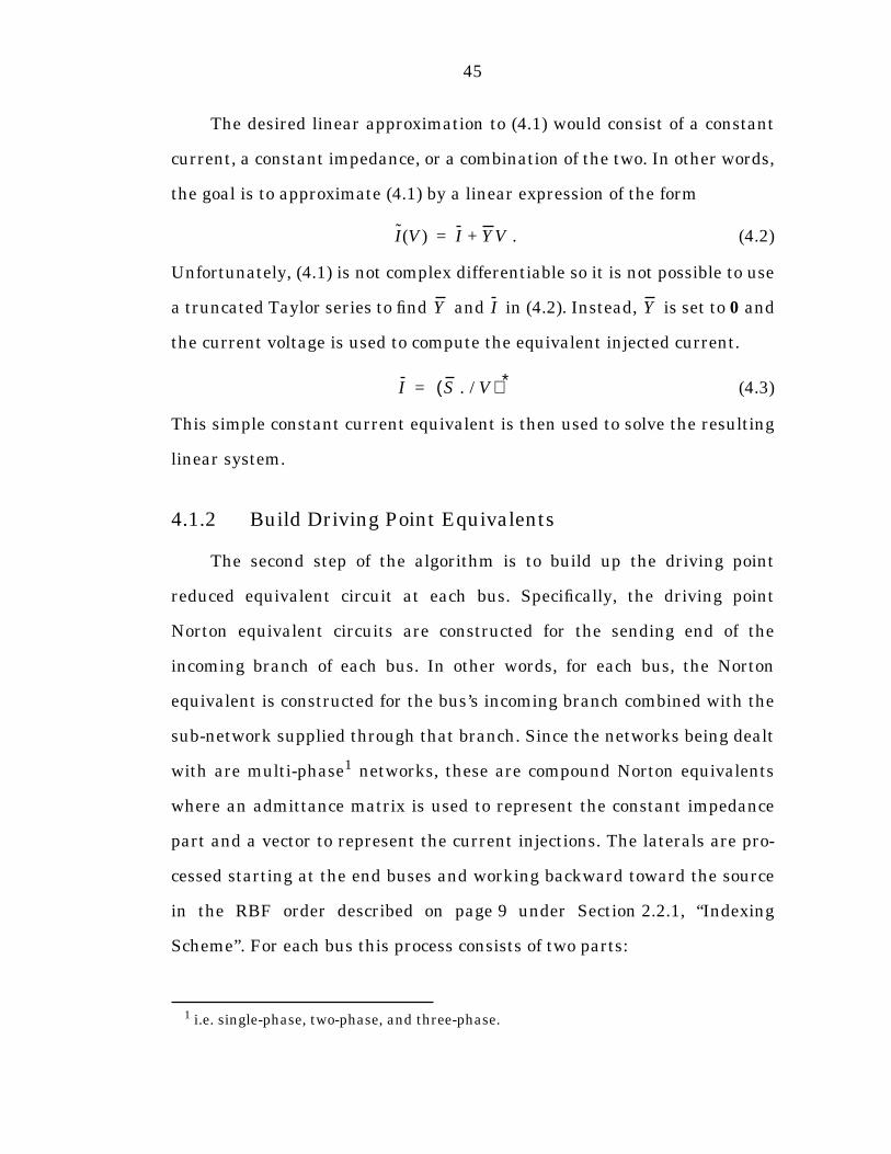
45

The desired linear approximation to (4.1) would consist of a constant

current, a constant impedance, or a combination of the two. In other words,

the goal is to approximate (4.1) by a linear expression of the form

. (4.2)

Unfortunately, (4.1) is not complex differentiable so it is not possible to use

a truncated Taylor series to find and in (4.2). Instead, is set to 0 and

the current voltage is used to compute the equivalent injected current.

(4.3)

This simple constant current equivalent is then used to solve the resulting

linear system.

4.1.2 Build Driving Point Equivalents

The second step of the algorithm is to build up the driving point

reduced equivalent circuit at each bus. Specifically, the driving point

Norton equivalent circuits are constructed for the sending end of the

incoming branch of each bus. In other words, for each bus, the Norton

equivalent is constructed for the bus’s incoming branch combined with the

sub-network supplied through that branch. Since the networks being dealt

with are multi-phase1 networks, these are compound Norton equivalents

where an admittance matrix is used to represent the constant impedance

part and a vector to represent the current injections. The laterals are pro-

cessed starting at the end buses and working backward toward the source

in the RBF order described on page 9 under Section 2.2.1, “Indexing

Scheme”. For each bus this process consists of two parts:

1 i.e. single-phase, two-phase, and three-phase.

I V( ) I YV+=

Y I Y

I S V. /( ) ∗=

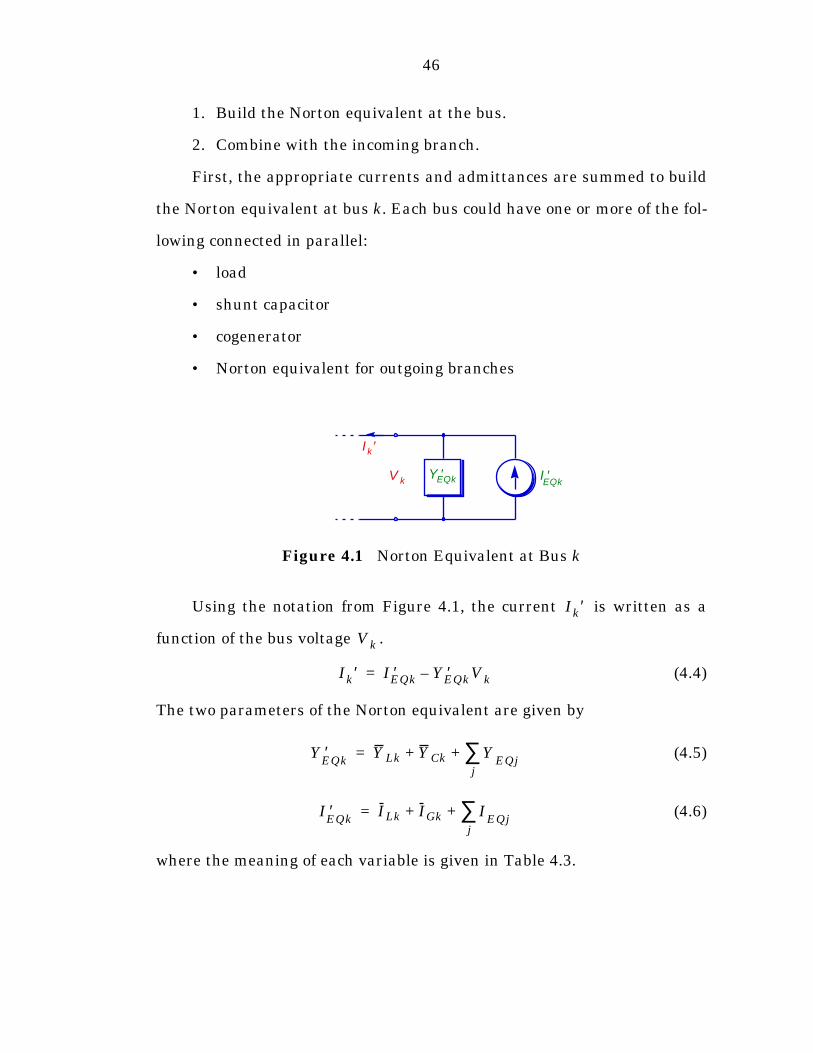
46

1. Build the Norton equivalent at the bus.

2. Combine with the incoming branch.

First, the appropriate currents and admittances are summed to build

the Norton equivalent at bus k. Each bus could have one or more of the fol-

lowing connected in parallel:

• load

• shunt capacitor

• cogenerator

• Norton equivalent for outgoing branches

Using the notation from Figure 4.1, the current is written as a

function of the bus voltage .

(4.4)

The two parameters of the Norton equivalent are given by

(4.5)

(4.6)

where the meaning of each variable is given in Table 4.3.

Figure 4.1 Norton Equivalent at Bus k

Y ′EQk I ′EQk

V k

I k ′

Ik′

Vk

Ik′ I ′EQk Y ′EQkVk–=

Y ′EQk

Y Lk YCk YEQj

j∑+ +=

I ′EQk

ILk IGk IEQj

j∑+ +=

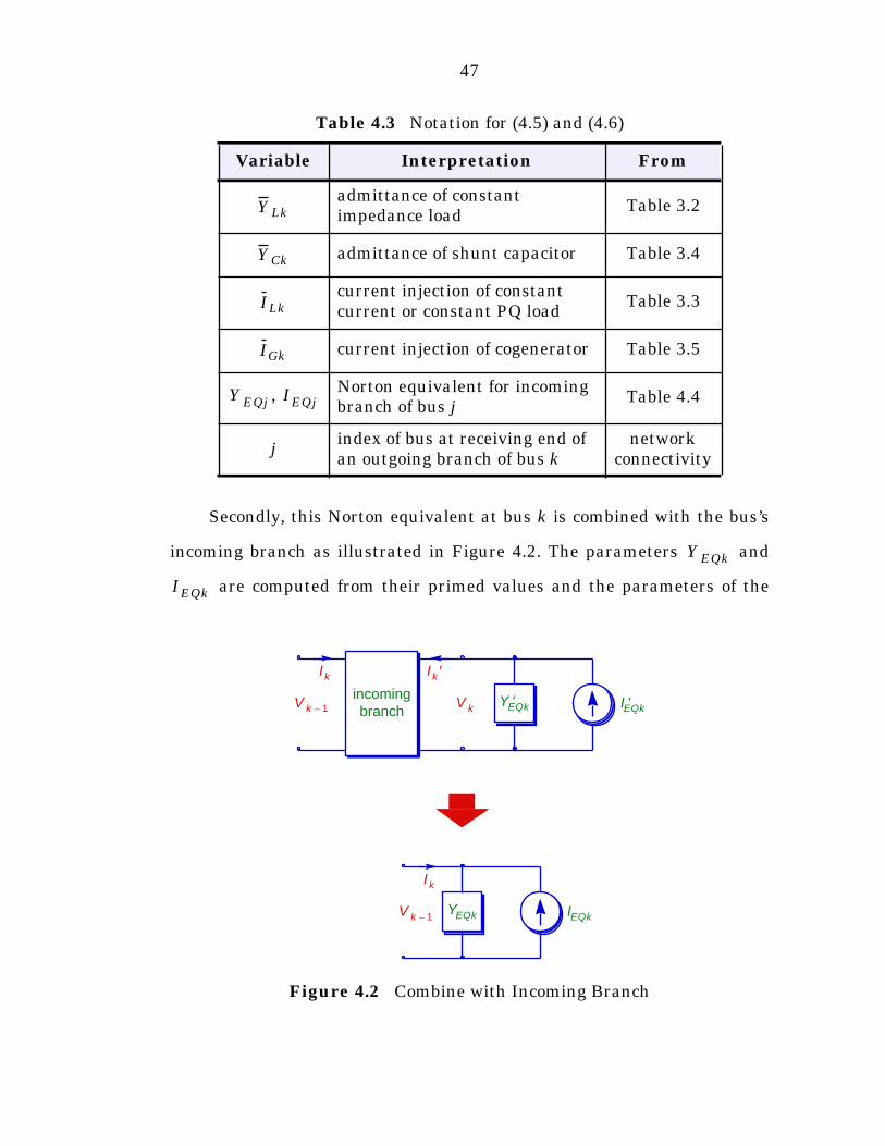
47

Secondly, this Norton equivalent at bus k is combined with the bus’s

incoming branch as illustrated in Figure 4.2. The parameters and

are computed from their primed values and the parameters of the

Table 4.3 Notation for (4.5) and (4.6)

Variable Interpretation From

admittance of constantimpedance load

Table 3.2

admittance of shunt capacitor Table 3.4

current injection of constant current or constant PQ load

Table 3.3

current injection of cogenerator Table 3.5

, Norton equivalent for incoming branch of bus j

Table 4.4

jindex of bus at receiving end of an outgoing branch of bus k

networkconnectivity

Figure 4.2 Combine with Incoming Branch

Y Lk

YCk

ILk

IGk

Y EQj IEQj

Y EQk

IEQk

YEQk IEQk

Y ′EQk I ′EQkV k

I k ′incomingbranch

I k

V k 1–

I k

V k 1–

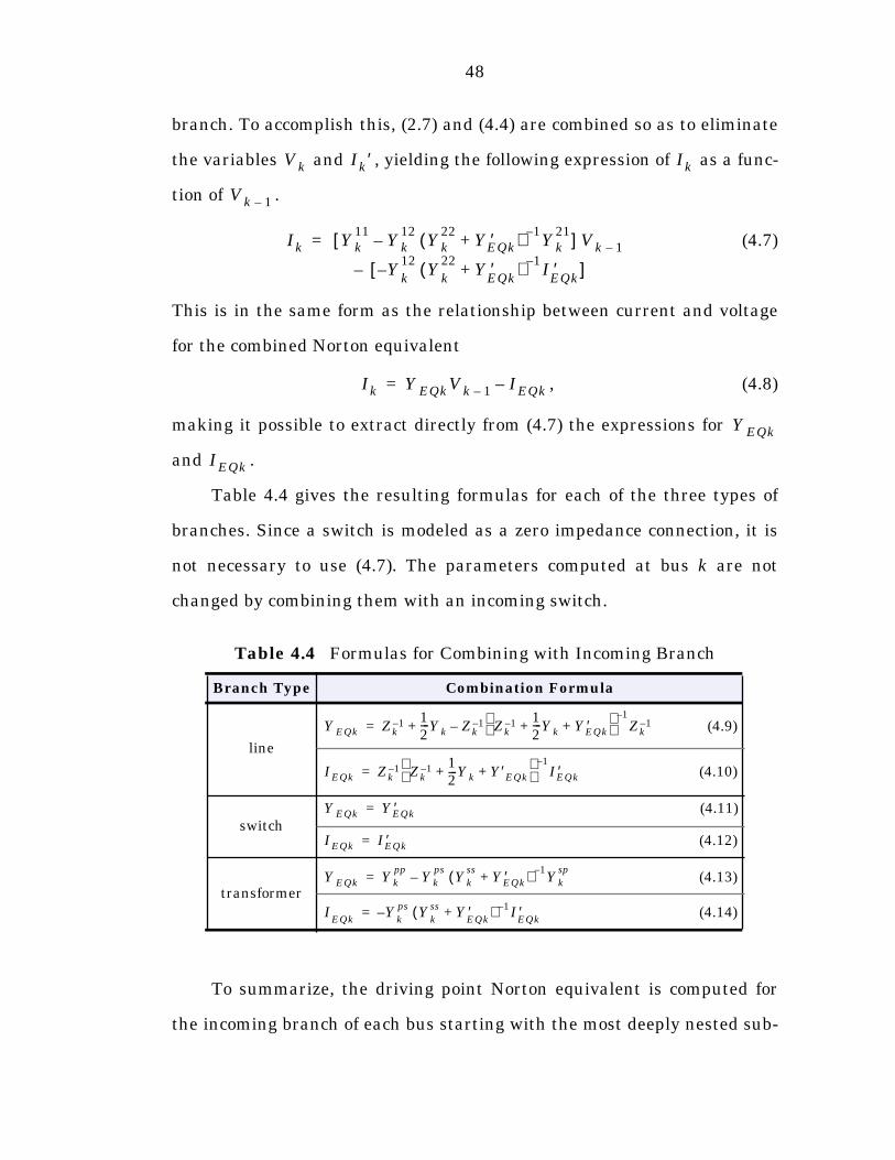
48

branch. To accomplish this, (2.7) and (4.4) are combined so as to eliminate

the variables and , yielding the following expression of as a func-

tion of .

(4.7)

This is in the same form as the relationship between current and voltage

for the combined Norton equivalent

, (4.8)

making it possible to extract directly from (4.7) the expressions for

and .

Table 4.4 gives the resulting formulas for each of the three types of

branches. Since a switch is modeled as a zero impedance connection, it is

not necessary to use (4.7). The parameters computed at bus k are not

changed by combining them with an incoming switch.

To summarize, the driving point Norton equivalent is computed for

the incoming branch of each bus starting with the most deeply nested sub-

Table 4.4 Formulas for Combining with Incoming Branch

Branch Type Combination Formula

line

(4.9)

(4.10)

switch(4.11)

(4.12)

transformer(4.13)

(4.14)

Vk Ik′ Ik

Vk 1–

Ik Yk11

Yk12

Yk22

Y ′EQk+( ) 1–Yk

21–[ ] Vk 1–

Yk12

Yk22

Y ′EQk

+( ) 1–I ′

EQk–[ ]–

=

Ik Y EQkVk 1– IEQk–=

Y EQk

IEQk

Y EQk Zk1– 1

2---Yk Zk

1– Zk1– 1

2---Yk Y ′EQk+ +

1–Zk

1––+=

IEQk Zk1– Zk

1– 12---Yk Y′EQk+ +

1–I ′EQk=

Y EQk Y ′EQk=

IEQk I ′EQk=

Y EQk Ykpp

Ykps

Ykss

Y ′EQk+( ) 1–Yk

sp–=

IEQk

Ykps Y

kss Y ′

EQk+( ) 1– I ′

EQk–=

49

laterals and working back toward the main feeder. At each bus the proce-

dure consists of two parts. First, all of the current sources and admittances

connected in parallel at the bus are summed together to give the Norton

equivalent at the bus for the part of the network supplied through that

bus. Then, this Norton equivalent is combined with the incoming branch to

determine the driving point Norton equivalent for that branch. At the end

of this second step of the algorithm, the driving point Norton equivalent for

the incoming branch of each bus is known. In other words, any branch and

the sub-network it supplies may be replaced by its Norton equivalent for

the purposes of computation.

4.1.3 Calculate Voltages and Currents

The result of the second step of the algorithm given in Table 4.1 is

that, given the voltage at a bus, the current to each of its outgoing

branches can be easily computed from the corresponding driving point

equivalent. The third step of the algorithm is based on this result. It

involves starting at the source, where the voltage is known, and computing

voltages and currents toward the end buses.

Once again, the entire network is traversed, this time in the BF order

described on page 11 under Section 2.2.1, “Indexing Scheme”. As in the

previous step, at each bus there is a two part calculation to be performed.

First, the current is computed for the bus’s incoming branch, then the bus

voltage is updated. For bus k this means calculating then .

The new value of is computed directly from the voltage at bus

and the Norton equivalent associated with the incoming branch of bus k.

The formula is given in (4.8) which is repeated here.

Ik Vk

Ik k 1–

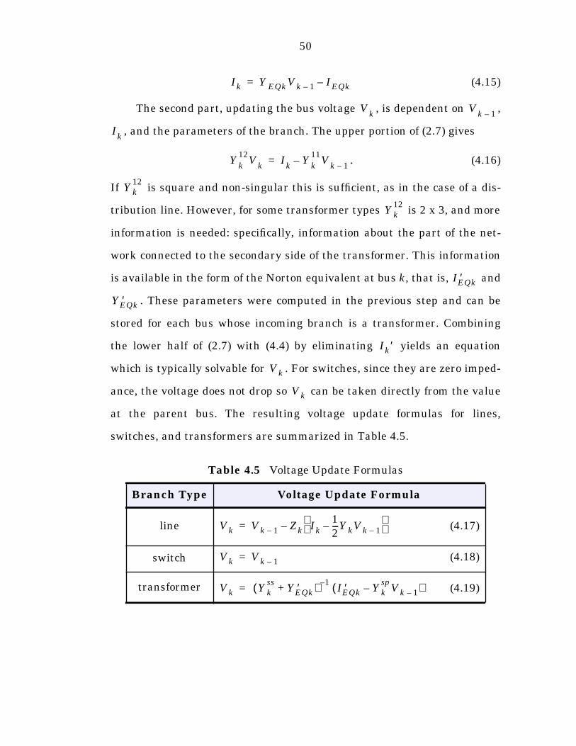
50

(4.15)

The second part, updating the bus voltage , is dependent on ,

, and the parameters of the branch. The upper portion of (2.7) gives

. (4.16)

If is square and non-singular this is sufficient, as in the case of a dis-

tribution line. However, for some transformer types is 2 x 3, and more

information is needed: specifically, information about the part of the net-

work connected to the secondary side of the transformer. This information

is available in the form of the Norton equivalent at bus k, that is, and

. These parameters were computed in the previous step and can be

stored for each bus whose incoming branch is a transformer. Combining

the lower half of (2.7) with (4.4) by eliminating yields an equation

which is typically solvable for . For switches, since they are zero imped-

ance, the voltage does not drop so can be taken directly from the value

at the parent bus. The resulting voltage update formulas for lines,

switches, and transformers are summarized in Table 4.5.

Table 4.5 Voltage Update Formulas

Branch Type Voltage Update Formula

line (4.17)

switch (4.18)

transformer (4.19)

Ik Y EQkVk 1– IEQk–=

Vk

Vk 1–

Ik

Yk12

Vk

Ik

Yk11

Vk 1––=

Yk12

Yk12

I ′EQk

Y ′EQk

Ik′

Vk

Vk

Vk Vk 1– Zk Ik12---YkVk 1––

–=

Vk Vk 1–=

Vk Ykss

Y ′EQk+( ) 1–I ′EQk Yk

spVk 1––( )=

51

4.1.4 Termination Criterion

The three steps, linearization, building driving point equivalents, and

computing voltages and currents, are repeated until convergence is

achieved. The algorithm is terminated when the norm of the change in

voltage from one iteration to the next is smaller than some predefined tol-

erance.2

4.2 Implementation

Several specific techniques can be used in the implementation of the

Norton reduction algorithm (N-PARS) to improve the efficiency and robust-

ness.

4.2.1 Linearity Check

It is conceivable that some networks do not contain any cogenerators

or constant PQ loads. In this case, the circuit is already a linear circuit.

Not only is the first step of the algorithm, linearization, unnecessary, but

there is no need to iterate. The circuit is solved directly in one iteration.

In the implementation, a check for non-linear components can be per-

formed at the beginning. If none are found, the program proceeds directly

to Norton reduction and terminates after one iteration. Without this check,

the program would do two iterations and find that there is no change

between iterations. The consequence of implementing this check is a 50%

savings in computation for linear networks.

2 Alternatively, the termination criterion could be based on the norm of the mismatchbetween the given power injection and the power injection computed from the voltage andcurrent injection at the current iteration.

52

4.2.2 Improved Line Update

The formulas given in (4.9) and (4.10) for combining the Norton equiv-

alent at bus k with its incoming line involve two matrix inversions. Inver-

sion of a matrix is an expensive operation in general, and may be ill-

conditioned as well, depending on the matrix.

The formulas below offer a more efficient and robust implementation.

They are equivalent to (4.9) and (4.10) but require less computation (only

one inverse instead of two) and are better conditioned for some line param-

eters.

(4.20)

(4.21)

Here I is the appropriately sized identity matrix.

4.2.3 Storage of Intermediate Variables

In the case where the circuit contains non-linear elements, the only

parameters which change from iteration to iteration are the currents

injected by these non-linear elements. In particular, as a new iteration

begins, only (for constant PQ loads) and in (4.6) take on new val-

ues based on the updated bus voltages. These changes affect only and

ultimately , but not and . These admittances remain con-

stant throughout all iterations and therefore need not be recomputed. This

means that (4.5), (4.9),3 (4.11), and (4.13) need only be computed once dur-

ing the first iteration.

3 Or (4.20) in actual implementation.

Y EQk12---Yk I

12---Yk Y ′EQk+

Zk+1–

+ 1

2---Yk Y ′EQk+

=

IEQk I12---Yk Y ′EQk+

Zk+1–I ′EQk=

ILk IGk

I ′EQk

IEQk

Y ′EQk

YEQk

53

A further savings in computation is achieved by storing the constant

coefficient of in (4.10)4 and (4.14). This reduces the second step of the

algorithm to a simple summation of the injected currents at a bus and

matrix-vector multiplication to combine with the bus’s incoming branch.

Saving these intermediate quantities and avoiding the recomputation

of the admittances is somewhat analogous to factoring Ybus only once and

saving it in a factored form in an Implicit Zbus Gauss type of power flow

algorithm such as those used in [9; 10; 27]. A more intelligent implementa-

tion could even detect areas of the network which do not contain constant

PQ elements and only perform the updates on the areas with quantities

which actually change.

4.3 Variations

There are other variations of the general network reduction power

flow method (NR-PARS) outlined in Table 4.1, “Network Reduction

Method”, on page 43. A method based on admittance equivalent only

(Y-PARS) was also implemented. Berg, Hawkins and Pleines initially pre-

sented a method based on this idea in [4], which has been extended to

include the more general modeling of Chapter 3.

Instead of Norton equivalent circuits, admittance equivalents are

used. The first step of the algorithm, linearization, now also includes con-

verting constant current elements to their constant impedance equiva-

lents. Constant current loads, constant PQ loads, and cogenerators are all

converted to the equivalent admittance via the formulas in Table 3.2 and

4 Or (4.21) in actual implementation.

I ′EQk

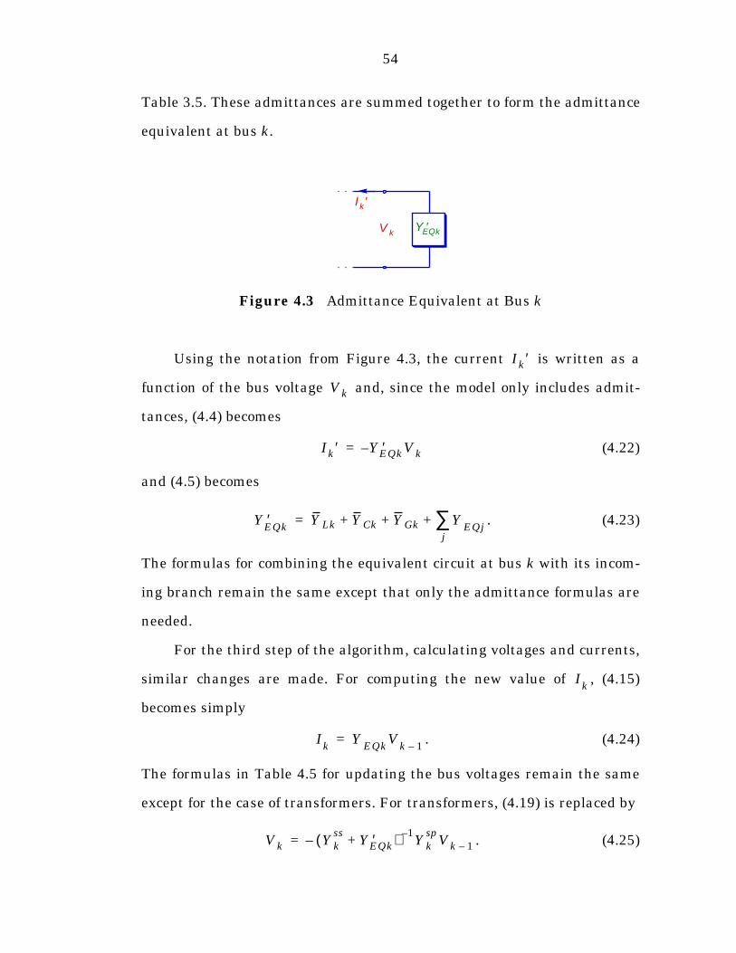
54

Table 3.5. These admittances are summed together to form the admittance

equivalent at bus k.

Using the notation from Figure 4.3, the current is written as a

function of the bus voltage and, since the model only includes admit-

tances, (4.4) becomes

(4.22)

and (4.5) becomes

. (4.23)

The formulas for combining the equivalent circuit at bus k with its incom-

ing branch remain the same except that only the admittance formulas are

needed.

For the third step of the algorithm, calculating voltages and currents,

similar changes are made. For computing the new value of , (4.15)

becomes simply

. (4.24)

The formulas in Table 4.5 for updating the bus voltages remain the same

except for the case of transformers. For transformers, (4.19) is replaced by

. (4.25)

Figure 4.3 Admittance Equivalent at Bus k

Y ′EQkV k

I k ′

Ik′

Vk

Ik′ Y ′EQkVk–=

Y ′EQk

Y Lk YCk YGk YEQj

j∑+ + +=

Ik

Ik

YEQk

Vk 1–=

Vk Ykss

Y ′EQk+( ) 1–Yk

spVk 1––=

55

Though the algorithm works fine, there seems to be little or no advan-

tage of Y-PARS over N-PARS. It is slightly more efficient for the case

where iteration is not necessary. However, the set of systems for which

iteration is not required has now been reduced to cases with no cogenera-

tors and only constant impedance loads. In the general iterative case, each

iteration requires all parameters to be recomputed. This is much more

computationally expensive than N-PARS implemented using the tech-

niques described in Section 4.2.3, “Storage of Intermediate Variables”.

4.4 Convergence Analysis

The convergence characteristics of N-PARS are exactly the same as

those of the familiar Z-matrix methods, including the Implicit Zbus Gauss

method [9; 10; 27]. Both N-PARS and the Z-matrix methods repeatedly

solve the linear circuit obtained by replacing all constant PQ devices with

their equivalent current injections at each iteration. In a circuit with no

constant power components, the solution is therefore obtained in a single

iteration and convergence is not an issue. For the more general case,

including constant power devices, convergence behavior is discussed in

[25]. The general conclusion is that convergence is best when load powers

are small, a condition which is met by the typical distribution system.

4.5 Comments

The power flow algorithms described in this chapter, particularly the

Norton reduction method (N-PARS), have several characteristics which

make them uniquely suited to certain situations. First of all, N-PARS is a

general method for solving the radial power flow problem which can handle

56

all of the transformer connection types listed in Table 3.8, “Admittance

Matrices for Common Transformer Connections”, on page 36. It is particu-

larly efficient for networks which contain no constant PQ elements.

The equivalent circuit parameters themselves, computed during the

solution process, may be useful for certain applications. They could be

used, for example, to replace a section of the network with a simple equiva-

lent linear model, while focusing on the effects of changes in another part

of the network.

Since the NR-PARS approaches exploit the radial structure of the net-

work, the work required for each iteration is proportional to the number of

buses. If the number of iterations remains constant, the work grows lin-

early with the size of the system, making NR-PARS suitable for very large

scale systems.

57

Chapter 5

Backward/Forward Sweep Power Flow Algorithms for Radial Systems (BFS-PARS)

One of the distinguishing features of the radial distribution network

is that there is a unique path from any given bus back to the source. This is

the key feature exploited by the backward/forward sweep class of algo-

rithms (BFS-PARS) presented in this chapter. These methods are based on

updating voltages and currents (or power flows) along these unique paths.

There are many variations to BFS-PARS. This chapter will first

present in detail a fairly general one, VI-VI-PARS, then discuss several

possible modifications which lead to the other variations. Several methods

based on the backward/forward sweep concept have been proposed by oth-

ers [3; 11; 18; 19; 20; 23]. In general, however, the approaches proposed in

the literature do not include the comprehensive modeling covered by the

general framework presented in this chapter. In fact, none of the methods

proposed in [3; 11; 18; 19; 20; 23] handle transformers of type 2, 3, 4, or 7.

In addition, [3; 19; 20; 23] only propose single-phase implementations,

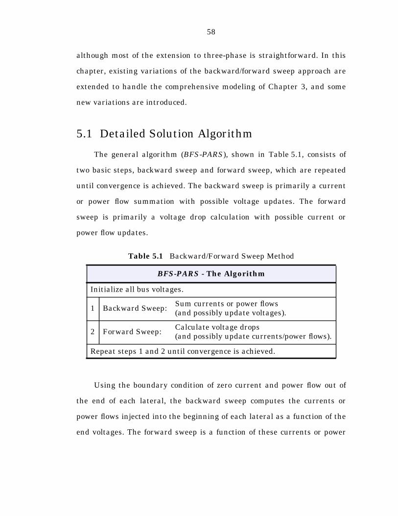
58

although most of the extension to three-phase is straightforward. In this

chapter, existing variations of the backward/forward sweep approach are

extended to handle the comprehensive modeling of Chapter 3, and some

new variations are introduced.


The general algorithm (BFS-PARS), shown in Table 5.1, consists of

two basic steps, backward sweep and forward sweep, which are repeated

until convergence is achieved. The backward sweep is primarily a current

or power flow summation with possible voltage updates. The forward

sweep is primarily a voltage drop calculation with possible current or

power flow updates.

Using the boundary condition of zero current and power flow out of

the end of each lateral, the backward sweep computes the currents or

power flows injected into the beginning of each lateral as a function of the

end voltages. The forward sweep is a function of these currents or power

Table 5.1 Backward/Forward Sweep Method

BFS-PARS - The Algorithm

Initialize all bus voltages.

1 Backward Sweep:Sum currents or power flows(and possibly update voltages).

2 Forward Sweep:Calculate voltage drops(and possibly update currents/power flows).

Repeat steps 1 and 2 until convergence is achieved.

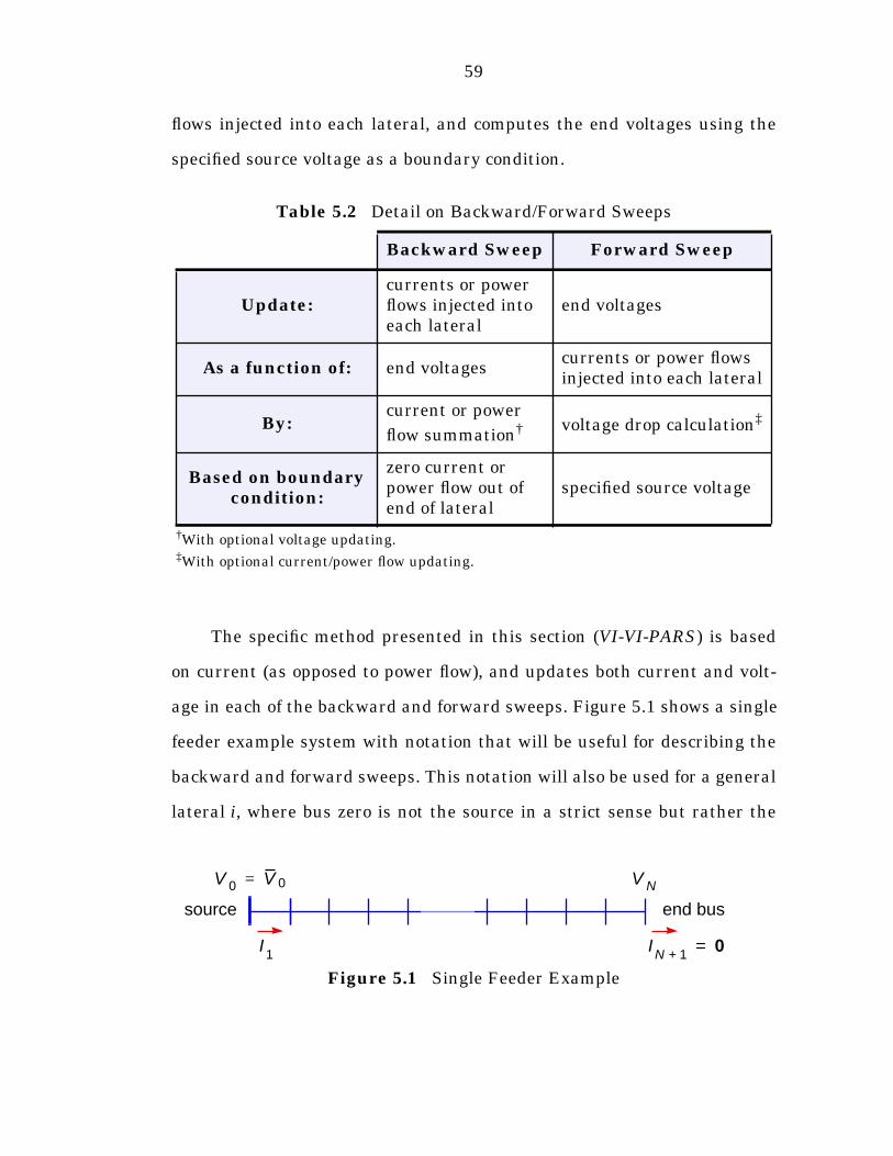
59

flows injected into each lateral, and computes the end voltages using the

specified source voltage as a boundary condition.

The specific method presented in this section (VI-VI-PARS) is based

on current (as opposed to power flow), and updates both current and volt-

age in each of the backward and forward sweeps. Figure 5.1 shows a single

feeder example system with notation that will be useful for describing the

backward and forward sweeps. This notation will also be used for a general

lateral i, where bus zero is not the source in a strict sense but rather the

†With optional voltage updating.‡With optional current/power flow updating.

Table 5.2 Detail on Backward/Forward Sweeps

Backward Sweep Forward Sweep

Update:currents or power flows injected into each lateral

end voltages

As a function of: end voltagescurrents or power flows injected into each lateral

By:current or power

flow summation† voltage drop calculation‡

Based on boundary condition:

zero current or power flow out of end of lateral

specified source voltage

Figure 5.1 Single Feeder Example

source

V 0 V 0= V N

I1 IN 1+ 0=

end bus

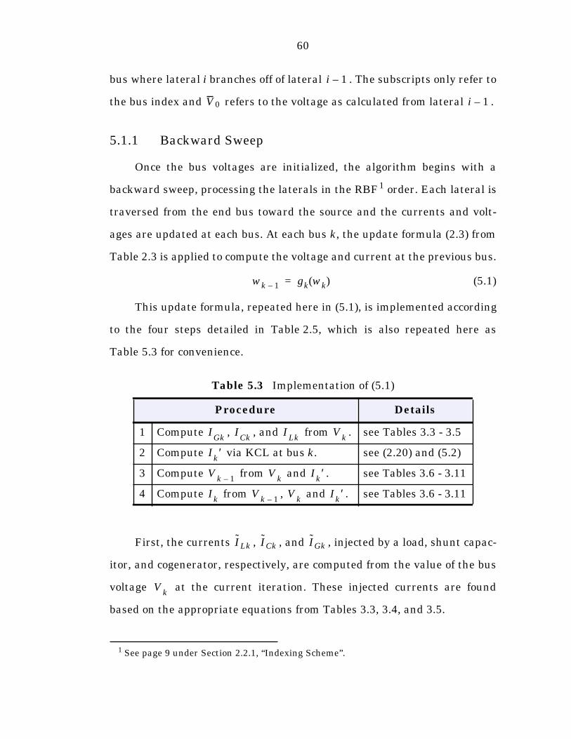
60

bus where lateral i branches off of lateral . The subscripts only refer to

the bus index and refers to the voltage as calculated from lateral .

5.1.1 Backward Sweep

Once the bus voltages are initialized, the algorithm begins with a

backward sweep, processing the laterals in the RBF1 order. Each lateral is

traversed from the end bus toward the source and the currents and volt-

ages are updated at each bus. At each bus k, the update formula (2.3) from

Table 2.3 is applied to compute the voltage and current at the previous bus.

(5.1)

This update formula, repeated here in (5.1), is implemented according

to the four steps detailed in Table 2.5, which is also repeated here as

Table 5.3 for convenience.

First, the currents , , and , injected by a load, shunt capac-

itor, and cogenerator, respectively, are computed from the value of the bus

voltage at the current iteration. These injected currents are found

based on the appropriate equations from Tables 3.3, 3.4, and 3.5.



Procedure Details


2 Compute via KCL at bus k. see (2.20) and (5.2)



i 1–

V0 i 1–

wk 1– gk wk( )=

IGk

ICk

ILk

Vk

Ik′

Vk 1– V

kI

k′

Ik

Vk 1– V

kI

k′

ILk ICk IGk

Vk

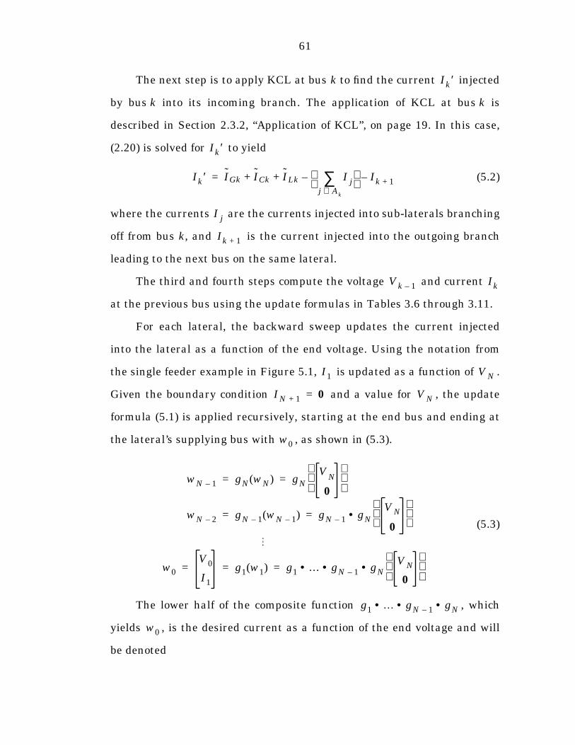
61

The next step is to apply KCL at bus k to find the current injected

by bus k into its incoming branch. The application of KCL at bus k is

described in Section 2.3.2, “Application of KCL”, on page 19. In this case,

(2.20) is solved for to yield

(5.2)

where the currents are the currents injected into sub-laterals branching

off from bus k, and is the current injected into the outgoing branch

leading to the next bus on the same lateral.

The third and fourth steps compute the voltage and current

at the previous bus using the update formulas in Tables 3.6 through 3.11.

For each lateral, the backward sweep updates the current injected

into the lateral as a function of the end voltage. Using the notation from

the single feeder example in Figure 5.1, is updated as a function of .

Given the boundary condition and a value for , the update

formula (5.1) is applied recursively, starting at the end bus and ending at

the lateral’s supplying bus with , as shown in (5.3).

(5.3)

The lower half of the composite function , which

yields , is the desired current as a function of the end voltage and will

be denoted

Ik′

Ik′

Ik′ IGk ICk ILk I jj Ak∈∑

– Ik 1+–+ +=

I j

Ik 1+

Vk 1– Ik

I1 V N

IN 1+ 0= V N

w0

wN 1– gN wN( ) gNV

N

0

= =

wN 2– gN 1– wN 1–( ) gN 1– gN•V N

0

= =

w0

V0

I1

g1 w1( ) g1 …• gN 1– gN•• V N

0

= = =

g1 …• gN 1– gN••

w0

62

. (5.4)

This value of the current is stored for use during the KCL calculation at

this lateral’s supplying bus during the current backward sweep and the

succeeding forward sweep. The upper half, which is the voltage part, is

, and is used only for mismatch calculation. At the solution, the

mismatch between the computed voltage and the

specified voltage must be zero.

To evaluate (5.4) for a given lateral, the currents injected into all of its

sub-laterals must be known, since they are needed for the application of

KCL in (5.2). This means the laterals must be processed in a specific order,

such as the RBF1 order used here. Since the level L laterals have no sub-

laterals, they are processed first. Next, the currents injected into the sub-

laterals of all level laterals are known, so the level laterals can

be processed. Each lateral is processed in this manner, starting with

level L, then moving to level , then , etc. Finally, the main feeder

is processed, completing the backward sweep. In the process, all voltages

and currents in the network are updated. In particular, the currents

injected into each lateral are updated as a function of the end voltages.

5.1.2 Forward Sweep

The second half of each iteration of the BFS-PARS algorithm is the

forward sweep which starts at the source and moves toward the end buses.

During the forward sweep, the laterals are processed in the BF2 order.


I1 I1 V N( )=

V0 V N( )

V0 V N( ) V0– V0 V N( )

V0

L 1– L 1–

L 1– L 2–

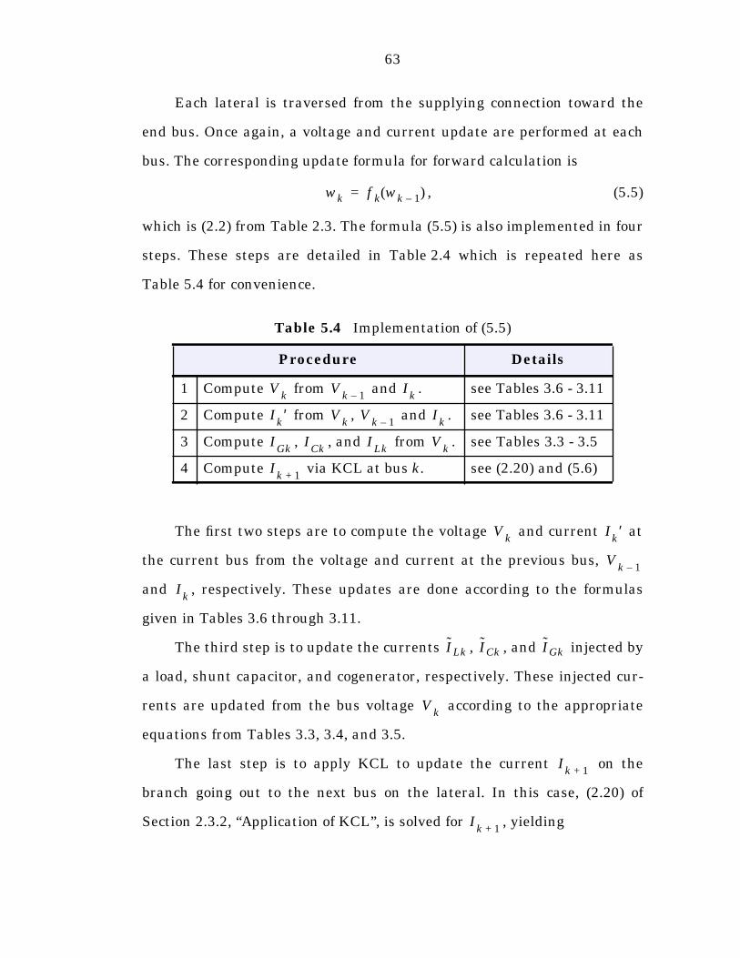
63

Each lateral is traversed from the supplying connection toward the

end bus. Once again, a voltage and current update are performed at each

bus. The corresponding update formula for forward calculation is

, (5.5)

which is (2.2) from Table 2.3. The formula (5.5) is also implemented in four

steps. These steps are detailed in Table 2.4 which is repeated here as

Table 5.4 for convenience.

The first two steps are to compute the voltage and current at

the current bus from the voltage and current at the previous bus,

and , respectively. These updates are done according to the formulas

given in Tables 3.6 through 3.11.

The third step is to update the currents , , and injected by

a load, shunt capacitor, and cogenerator, respectively. These injected cur-

rents are updated from the bus voltage according to the appropriate

equations from Tables 3.3, 3.4, and 3.5.

The last step is to apply KCL to update the current on the

branch going out to the next bus on the lateral. In this case, (2.20) of

Section 2.3.2, “Application of KCL”, is solved for , yielding


Procedure Details




4 Compute via KCL at bus k. see (2.20) and (5.6)

wk f k wk 1–( )=

Vk

Vk 1– I

k

Ik′ V

kV

k 1– Ik

IGk

ICk

ILk

Vk

Ik 1+

Vk

Ik′

Vk 1–

Ik

ILk ICk IGk

Vk

Ik 1+

Ik 1+

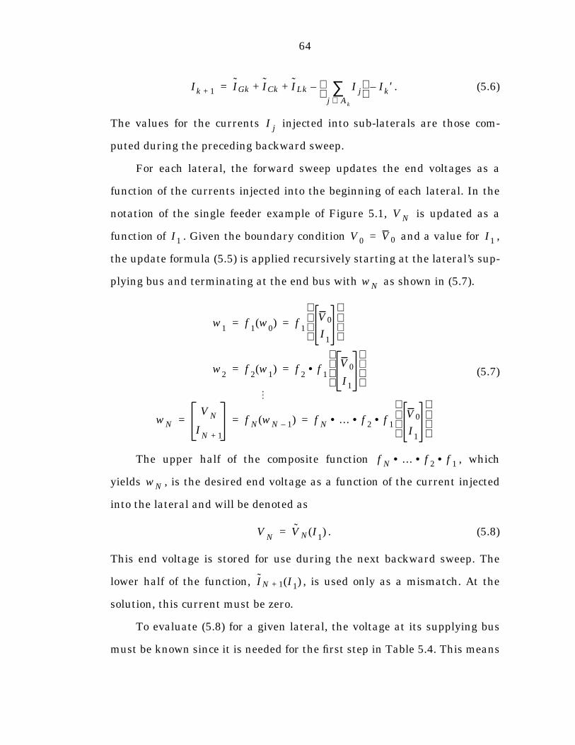
64

. (5.6)

The values for the currents injected into sub-laterals are those com-

puted during the preceding backward sweep.

For each lateral, the forward sweep updates the end voltages as a

function of the currents injected into the beginning of each lateral. In the

notation of the single feeder example of Figure 5.1, is updated as a

function of . Given the boundary condition and a value for ,

the update formula (5.5) is applied recursively starting at the lateral’s sup-

plying bus and terminating at the end bus with as shown in (5.7).

(5.7)

The upper half of the composite function , which

yields , is the desired end voltage as a function of the current injected

into the lateral and will be denoted as

. (5.8)

This end voltage is stored for use during the next backward sweep. The

lower half of the function, , is used only as a mismatch. At the

solution, this current must be zero.

To evaluate (5.8) for a given lateral, the voltage at its supplying bus

must be known since it is needed for the first step in Table 5.4. This means

Ik 1+ IGk ICk ILk I jj Ak∈∑

– Ik′–+ +=

I j

V N

I1 V0 V0= I1

wN

w1

f1

w0

( ) f1

V0

I1

= =

w2

f2

w1

( ) f2

f1

• V0

I1

= =

wN

V N

IN 1+

f N wN 1–( ) f N …• f 2 f 1•• V0

I1

= = =

f N …• f 2 f 1••

wN

VN

V N I1

( )=

IN 1+ I1( )

65

the laterals must be processed in a specific order, such as the BF2 order

used here. Since the source voltage is given, the main feeder is processed

first. Then, since the voltages at the supplying buses for all level 2 laterals

are known, the level 2 laterals can be processed, followed by level 3, etc.

Each lateral is processed in this manner until all the level L laterals have

been updated, completing the forward sweep. In the process, all voltages

and currents in the network are updated. In particular, all of the end volt-

ages are updated as a function of the currents injected into each lateral.


The backward and forward sweeps are repeated until convergence is

achieved. There are several ways of detecting convergence. The voltage

mismatches at the beginning of each lateral, calculated dur-

ing the backward sweep, must be zero at the solution. Likewise, the cur-

rent mismatches at the ends of the laterals, computed during the

forward sweep, must also be zero. Requiring that the norm of either of

these mismatches be smaller than some tolerance is a suitable termination

criterion.

It is also possible to use the termination criterion used for the net-

work reduction methods of Chapter 4. This approach requires that the

norm of the difference in bus voltages between iterations be smaller than a

given tolerance. In fact, this is the only one of the three approaches which

is suitable for some of the variations of BFS-PARS.

V0 V N( ) V0–

IN 1+ I1( )

66

5.2 Implementation

For the most part, the implementation of BFS-PARS is very straight-

forward. Special attention, however, is needed for laterals which contain

the class B and class C transformers. In particular, in step 3 of Table 5.3

and step 1 of Table 5.4 it is necessary to make some modifications to the

standard backward and forward sweeps described above. Consider lateral i

whose first bus k has a transformer as its incoming branch.3

5.2.1 Class B Transformers

Transformers of class B have three dimensional voltages and currents

on the primary side, while these quantities at the secondary side are two

dimensional. These transformers are described in detail in Section 3.6.2,

“Class B: Grounded Primary—Ungrounded Secondary”, where the rele-

vant update formulas are given in Table 3.10.

5.2.1.1 Backward Sweep

In step 3 of Table 5.3, the primary voltage is being computed from the

secondary voltage and current. For class B transformers, the correspond-

ing update formula is

(5.9)

from (3.52) in Table 3.10. As explained in Section 3.6.2, “Class B: Grounded

Primary—Ungrounded Secondary”, it is only possible to solve for if it

3 Due to the implementation explained in Section 2.2.2.2, “Breadth-First Search”, trans-formers always appear as the first branch on a lateral.

Vk 1–Yk

sp

1 1 1

1–

Ik′ Ykss

Vk–

Vk 1–Σ

=

Vk 1–

67

is assumed that some information is already given, such as the sum

of the primary side voltages.

Since (5.9) assumes that is available, BFS-PARS must provide

a reasonable estimate which becomes more accurate at each iteration as

the algorithm moves toward convergence. The sum of the primary side

voltage computed during the previous forward sweep provides such an esti-

mate and is stored as for use during the backward sweep. For the

first iteration, the initial primary voltage is used to compute . For the

typical flat start, with all voltages assumed to be balanced 1 per unit, this

yields .

For a lateral with a class B transformer, the typical backward sweep

function of (5.4) is a function of as well as .

(5.10)

Since, in this case, is 2 x 1, this is still a 3 x 1 function of three vari-

ables.

5.2.1.2 Forward Sweep

During the forward sweep, step 1 of Table 5.4 computes the secondary

voltage from the primary voltage and current. The corresponding update

formula for class B transformers is

(5.11)

from (3.50) in Table 3.10. As explained in Section 3.6.2, “Class B: Grounded

Primary—Ungrounded Secondary”, this formula yields a unique solution

Vk 1–Σ

Vk 1–Σ

Vk 1–Σ

Vk 1–Σ

Vk 1–Σ

0=

Vk 1–Σ

V N

I1 I1

V N

Vk 1–Σ

=

V N

Vk Ykps

Ik Ykpp

Vk 1––( )\=

68

for the secondary voltage only if the sum of the primary side currents

meets the appropriate constraint in (3.45) or (3.46).

Since the primary side current computed during the forward sweep

does not, in general, satisfy the appropriate constraint, must be modi-

fied to meet the constraint before using it in (5.11). The value used in (5.11)

should be as close to the computed as possible while meeting the neces-

sary constraint.

A reasonable approximation to this closest point can be found by add-

ing or subtracting equal values from each element of to satisfy the con-

straint. This is done by computing the constraint mismatch, which is

(5.12)

for type 2 grounded wye to ungrounded wye transformers and

(5.13)

for type 3 grounded wye to delta transformers. A third of this mismatch is

then subtracted from each element of to give a new which satisfies

the relevant constraint and can be used in (5.11) to compute .

(5.14)

The modified update formula, including the adjustment to the primary side

current , can be written in a closed form as

. (5.15)

Vk

IkΣ

Ik

Ik

Ik

IkΣ∆ Ik

Σ=

IkΣ∆ Ik

Σ yk

αk2

------Vk 1–Σ

–=

Ik

Ik

Vk

Ik Ik

IkΣ∆

3---------

11

1

–←

Ik

Vk Ykps

Ik

IkΣ∆

3---------

1

11

– Ykpp

Vk 1––\=

69

This small modification to allows the forward sweep to continue.

The typical forward sweep function of (5.8) is modified to reflect the impor-

tance of the update to which must be stored for the backward sweep.

(5.16)

Again, this is still a three dimensional function of three variables. A three

dimensional mismatch can also be formed by taking the constraint mis-

match along with the current out of the end of the lateral,

which in this case is 2 x 1.

The relatively small adjustment to the primary side current, shown in

(5.14), produces secondary side voltages and currents which are consistent

with the primary side current constraint. During the succeeding backward

sweep, these updated voltages produce a primary side current which more

closely meets the constraint.

5.2.2 Class C Transformers

Transformers of class C have three dimensional voltages and currents

on the secondary side, while these quantities at the primary side are two

dimensional. These transformers are described in detail in Section 3.6.3,

“Class C: Ungrounded Primary—Grounded Secondary”, where the rele-

vant update formulas are given in Table 3.11.

5.2.2.1 Forward Sweep

For class C transformers, step 1 of Table 5.4 during the forward sweep

is similar to the backward sweep for class B transformers. The relevant

update formula is

Ik

Vk 1–Σ

V N

Vk 1–Σ

V N I1

( )

Vk 1–Σ

I1( )=

IkΣ∆ IN 1+ I1( )

70

(5.17)

from (3.61) in Table 3.11. Once again, additional information is needed for

the evaluation of in (5.17). This additional information at the second-

ary side of the transformer must come from the previous backward sweep.

Since the backward sweep is based on a boundary condition of zero end

current, it is current information that is available at the transformer sec-

ondary. As explained in Section 3.6.3, “Class C: Ungrounded Primary—

Grounded Secondary”, this eliminates type 4 ungrounded wye to grounded

wye transformers which have no direct relationship between and .

Consequently, (5.17) is only valid for type 7 delta to grounded wye

transformers and the rest of this discussion of the handling of class C

transformers will be restricted to this type. Since it was computed during

the previous backward sweep, the sum of the secondary side current is

available for the evaluation of (5.17). The typical forward sweep function of

(5.8), for a lateral with a class C transformer, becomes

, (5.18)

where is 3 x 1, is 2 x 1, and is a scalar.

5.2.2.2 Backward Sweep

The backward sweep is similar to the forward sweep for class B trans-

formers. The relevant update formula for step 3 of Table 5.3 is

(5.19)

VkYk

ps

1 1 1

1–Ik Yk

ppVk 1––

βk2

yk------Ik

Σ′=

Vk

IkΣ′ Vk

Σ

IkΣ′

VN

V N

I1

IkΣ′

=

V N I1 IkΣ′

Vk 1– Yksp

Ik′ Ykss

Vk–( )\=

71

from (3.63) in Table 3.11, which requires that the constraint in (3.59) be

satisfied. Since the secondary voltage and current sums computed in the

current backward sweep typically do not meet this constraint, some modifi-

cation is required to proceed with the backward sweep. The forward sweep

requires an accurate value for so it is stored as is and the voltage is

chosen for adjustment.

First, a constraint mismatch is computed.

(5.20)

A third of this mismatch is then subtracted from each element of to

give a new value which satisfies (3.59) and can be used to solve for in

(5.19).

(5.21)

The modified update formula, including the adjustment to the secondary

side voltage , can be written in a closed form as

. (5.22)

This small change in allows the backward sweep to continue. The

typical backward sweep function of (5.4) is modified to reflect the impor-

tance of the update to which must be stored for the forward sweep.

(5.23)

IkΣ′ Vk

VkΣ∆ Vk

Σ βk2

yk

------IkΣ′–=

Vk

Vk 1–

Vk Vk

VkΣ∆

3-----------

1

1

1

–←

Vk

Vk 1– Yksp

Ik′ Ykss

Vk

VkΣ β

k2

yk------Ik

Σ′–

3----------------------------

1

1

1

–

–\=

Vk

IkΣ′

I1

IkΣ′

I1 V N( )

IkΣ

′ VN

( )=

72

Both the function and the independent variable are still 3 x 1. A three

dimensional mismatch is also formed by combining the constraint mis-

match of (5.20) with the two dimensional voltage mismatch at the

beginning of the lateral, .

The relatively small adjustment to the secondary side voltage, shown

in (5.21), produces primary side voltages and currents which are consistent

with the secondary side constraint. During the next forward sweep these

updated currents produce a secondary voltage which more closely meets

the constraint.

5.3 Variations

There are many variations to the general BFS-PARS of Table 5.1 and

Table 5.2. Some are based on current and others on power flow. Some

update voltages during the backward sweep and some do not. Some update

currents or power flows during the forward sweep and some do not. The

naming convention used for the various methods indicates first the vari-

ables updated during the forward sweep, then those updated during the

backward sweep. V is used for voltage, I for current, and S for power flow.

5.3.1 VI-VI-PARS

VI-VI-PARS is the particular variation described in detail in the pre-

ceding sections. It is based on current and it updates both voltages and

currents in both the backward and forward sweeps.

V N

VkΣ∆

V0 V N( ) V0–

73

5.3.2 VS-VS-PARS

VS-VS-PARS modifies the VI-VI-PARS approach, presented in detail

in foregoing sections of this chapter, by using power flow rather than cur-

rent. The approach presented in [3] is based on the same idea. The back-

ward sweep computes the power flow injected into each lateral as a

function of the end voltages by starting with the boundary condition of zero

power flow out of the end of the laterals. The forward sweep starts with the

specified source voltage as a boundary condition and computes the end

voltages as a function of the power injected into each lateral. At each step

of the algorithm, where a current is used in VI-VI-PARS, the corresponding

power flow is used in VS-VS-PARS. The update function used at each bus

during the backward sweep is (2.5) instead of (2.3), and for the forward

sweep it is (2.4) instead of (2.2).

The class B and class C transformers are the only exception to the

change from current to power flow. They are still handled exactly as

described in Section 5.2.1, “Class B Transformers”, and Section 5.2.2,

“Class C Transformers”. Due to the fact that the constraints are con-

straints on current and voltage, power flows are converted to the equiva-

lent currents and these currents are used as described. For instance, for

class B transformers during the forward sweep these currents are adjusted

as in (5.14). Likewise, the power at the secondary of class C transformers

during the backward sweep is converted to the equivalent current and

stored for use during the forward sweep. Hence, (5.18) becomes

(5.24)V N V N

S1

IkΣ′

=

74

and (5.23) becomes

(5.25)

There are two essential differences between VS-VS-PARS and

VI-VI-PARS. One difference has to do with computational efficiency.

VS-VS-PARS typically requires more computation than VI-VI-PARS. Only

certain parts of the calculation, such as the computation of the power and

current injections, respectively, for constant PQ loads are more efficient in

VS-VS-PARS. Even in networks with all constant PQ loads these gains are

more than offset by the increase in computation for other operations such

as voltage drop calculation.

The other essential difference in VS-VS-PARS is that the current

injected into each lateral changes from the time is com-

puted during the backward sweep to the time is used during the for-

ward sweep. In VI-VI-PARS the current is held constant between the

time it is computed in the backward sweep and the time it is used in the

forward sweep. In VS-VS-PARS, it is the power that is held constant

and the current changes depending on the change in the voltage.

Although this does not seem to have a significant effect on convergence, the

sequence of iterates does differ for the two algorithms.

The voltage mismatch at the beginning of each lateral calculated dur-

ing the backward sweep is the same as the voltage mismatch computed by

VI-VI-PARS. The forward sweep yields power mismatches at the end of

each lateral instead of current mismatches.

S1

IkΣ′

S1 V N( )

IkΣ

′ VN

( )=

S1 V0. /( ) ∗ S1

S1

I1

S1

I1

75

5.3.3 V-VI-PARS

This variation is identical to VI-VI-PARS in the backward sweep. The

forward sweep updates only voltages. A method based on a slightly modi-

fied version of this idea was proposed in [18]. Table 5.4 shows the proce-

dure performed at each bus during the forward sweep when both voltages

and currents are updated. In V-VI-PARS, steps 2, 3, and 4 are not per-

formed. The value used for in step 1 is the value computed during the

previous backward sweep. For this method, it is necessary to store this cur-

rent for each bus during the backward sweep. For VI-VI-PARS, it is only

necessary to store the currents injected into each lateral, not the currents

at each bus.

For class B transformers it is still necessary to modify during the

forward sweep according to (5.14) in order to satisfy the appropriate con-

straint in (3.45) or (3.46).

Since the currents are not updated in the forward sweep, the current

mismatch at the end of each lateral is not available as a termination crite-

rion for this method.

5.3.4 V-VS-PARS

V-VS-PARS is the power flow based counterpart to V-VI-PARS. The

backward sweep is identical to that of VS-VS-PARS and the forward sweep

updates only voltages based on the power flow values computed during

the backward sweep.

Since no power flows are updated during the forward sweep, there are

no power mismatches available at the ends of the laterals for use as a ter-

mination criterion.

Ik

Ik

Sk

76

5.3.5 VI-I-PARS

The forward sweep in this variation is identical to that of VI-VI-PARS.

The backward sweep, however, does not update voltages, only currents. In

Table 5.3, which details the procedure at each bus during the backward

sweep, step 3 is skipped. For step 4, is computed using values of voltage

computed in the previous forward sweep.

For class C transformers, it is still necessary to modify the secondary

voltage during the backward sweep according to (5.21) in order to sat-

isfy the constraint in (3.59).

Since no voltages are updated during the backward sweep, the voltage

mismatch at the beginning of each lateral is not available as a termination

criterion for this method.

5.3.6 VS-S-PARS

This is the power flow based version of VI-I-PARS. The forward sweep

is identical to that of VS-VS-PARS, but the backward sweep, like

VI-I-PARS, does not update voltages. Voltage values from the previous for-

ward sweep are used where needed. Once again, no voltage mismatch is

available as a termination criterion for this method.

5.3.7 V-I-PARS

V-I-PARS uses the backward sweep of VI-I-PARS, which updates only

currents, and the forward sweep of V-VI-PARS, which updates only volt-

ages. The methods proposed in [11] and [23] are based on this concept of

simple current summation in the backward sweep and voltage drop calcu-

lation in the forward sweep.

Ik

Vk

77

This method computes neither current nor voltage mismatches, and

the only convergence criterion available, of the three presented in

Section 5.1.3, “Termination Criterion”, is the one based on the difference in

voltage between iterations.

5.3.8 V-S-PARS

V-S-PARS is the power flow based counterpart to V-I-PARS, using the

backward sweep of VS-S-PARS and the forward sweep of V-VS-PARS. This

method uses simple power flow summation for the backward sweep and

voltage drop calculation for the forward sweep, which is also the basis for

the methods proposed in [19] and [20].


In this section, the convergence of V-I-PARS is considered for a distri-

bution system with no ungrounded sections. Some necessary notation for

the proof is given below in Table 5.5. With this notation, the backward

sweep can be summarized by the following two equations:

(5.26)

(5.27)

The forward sweep can be summarized by the following two equations:

(5.28)

(5.29)

where the initial node voltages at each bus are set to the corresponding

source voltage. Combining these four equations gives an expression for the

Ink( )

In YV nk( )

f Vnk( )

( )+ +=

Ib

k( )A

TI

nk( )

=

Vbk 1+( )

ZIbk( )

=

Vnk 1+( )

Vn0( )

AV bk 1+( )

–=

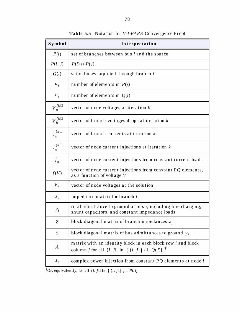
78

†Or, equivalently, for all in .

Table 5.5 Notation for V-I-PARS Convergence Proof

Symbol Interpretation

set of branches between bus i and the source

set of buses supplied through branch i

number of elements in

number of elements in

vector of node voltages at iteration k

vector of branch voltages drops at iteration k

vector of branch currents at iteration k

vector of node current injections at iteration k

vector of node current injections from constant current loads

vector of node current injections from constant PQ elements, as a function of voltage V

vector of node voltages at the solution

impedance matrix for branch i

total admittance to ground at bus i, including line charging, shunt capacitors, and constant impedance loads

Z block diagonal matrix of branch impedances

Y block diagonal matrix of bus admittances to ground

Amatrix with an identity block in each block row i and block

column j for all in †

complex power injection from constant PQ elements at node i

P i( )

P i j,( ) P i( ) P j( )∩

Q i( )

di P i( )

bi Q i( )

Vnk( )

Vbk( )

Ibk( )

Ink( )

In

f V( )

V*

zi

yi

zi

yi

i j,( ) i j,( ) i Q j( )∈{ }

si

i j,( ) i j,( ) j P i( )∈{ }

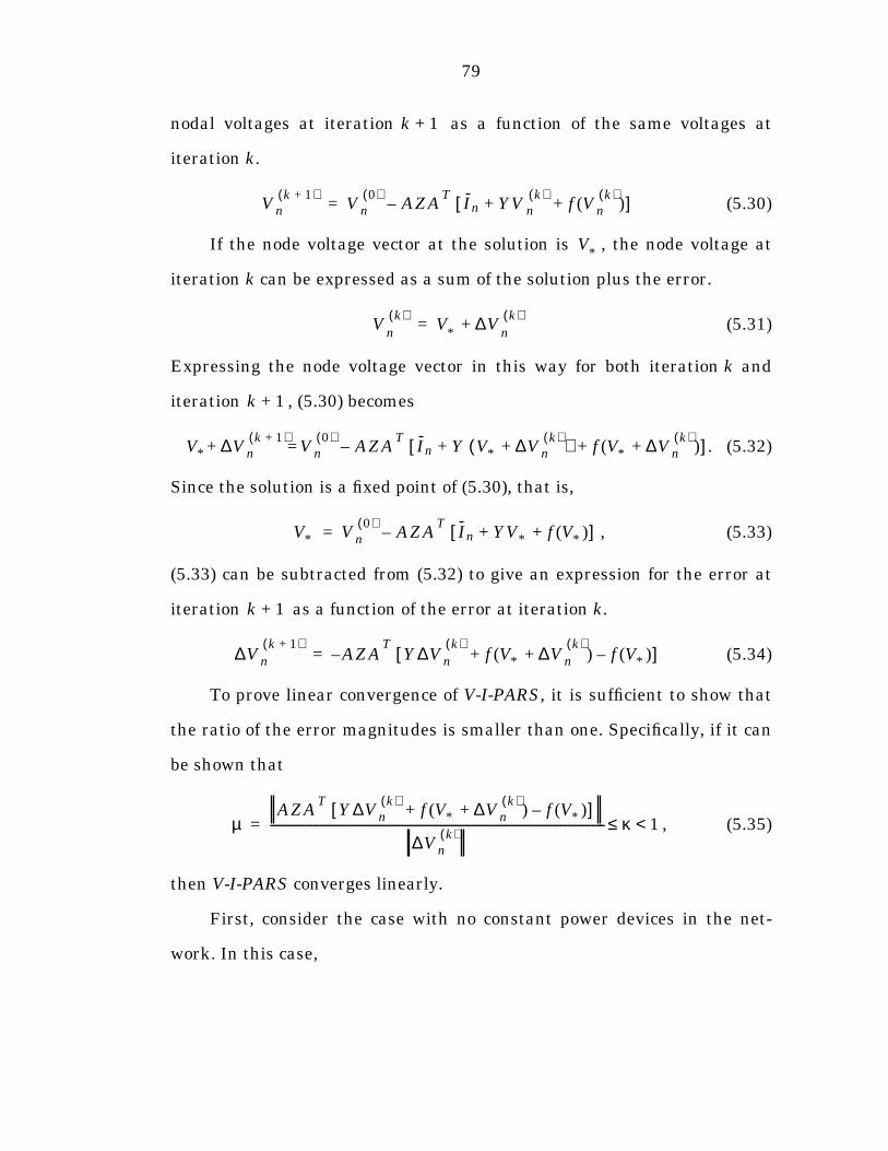
79

nodal voltages at iteration as a function of the same voltages at

iteration k.

(5.30)

If the node voltage vector at the solution is , the node voltage at

iteration k can be expressed as a sum of the solution plus the error.

(5.31)

Expressing the node voltage vector in this way for both iteration k and

iteration , (5.30) becomes

. (5.32)

Since the solution is a fixed point of (5.30), that is,

, (5.33)

(5.33) can be subtracted from (5.32) to give an expression for the error at

iteration as a function of the error at iteration k.

(5.34)

To prove linear convergence of V-I-PARS, it is sufficient to show that

the ratio of the error magnitudes is smaller than one. Specifically, if it can

be shown that

, (5.35)

then V-I-PARS converges linearly.

First, consider the case with no constant power devices in the net-

work. In this case,

k 1+

Vnk 1+( )

Vn0( )

AZAT

In YV nk( )

f Vnk( )

( )+ +[ ]–=

V*

Vn

k( )V

*∆V

nk( )

+=

k 1+

V* ∆Vnk 1+( )

+ Vn0( )

AZAT

In Y V* ∆Vnk( )

+( ) f V* ∆Vnk( )

+( )+ +[ ]–=

V* Vn0( )

AZAT

In YV* f V*( )+ +[ ]–=

k 1+

∆Vnk 1+( )

AZAT

Y∆Vnk( )

f V* ∆Vnk( )

+( ) f V*( )–+[ ]–=

µAZA

TY∆Vn

k( )f V* ∆Vn

k( )+( ) f V*( )–+[ ]

∆Vnk( )

------------------------------------------------------------------------------------------------------------------- κ 1<≤=

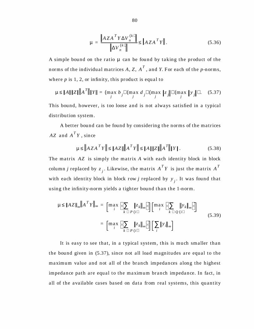
80

. (5.36)

A simple bound on the ratio can be found by taking the product of the

norms of the individual matrices A, Z, , and Y. For each of the p-norms,

where p is 1, 2, or infinity, this product is equal to

. (5.37)

This bound, however, is too loose and is not always satisfied in a typical

distribution system.

A better bound can be found by considering the norms of the matrices

and , since

. (5.38)

The matrix is simply the matrix A with each identity block in block

column j replaced by . Likewise, the matrix is just the matrix

with each identity block in block row j replaced by . It was found that

using the infinity-norm yields a tighter bound than the 1-norm.

(5.39)

It is easy to see that, in a typical system, this is much smaller than

the bound given in (5.37), since not all load magnitudes are equal to the

maximum value and not all of the branch impedances along the highest

impedance path are equal to the maximum branch impedance. In fact, in

all of the available cases based on data from real systems, this quantity

µAZA

TY∆Vn

k( )

∆Vnk( )

-------------------------------------------- AZAT

Y≤=

µ

AT

µ A Z AT

Y bjj

max ( ) djj

max ( ) zjj

max ( ) yjj

max ( )=≤

AZ AT

Y

µ AZAT

Y AZ AT

Y A Z AT

Y≤ ≤ ≤

AZ

zj

AT

Y AT

yj

µ AZ ∞ AT

Y ∞≤ zk ∞k P i( )∈∑

i

max yk ∞k Q i( )∈∑

i

max

zk ∞k P i( )∈∑

i

max yi ∞i

∑

=

=

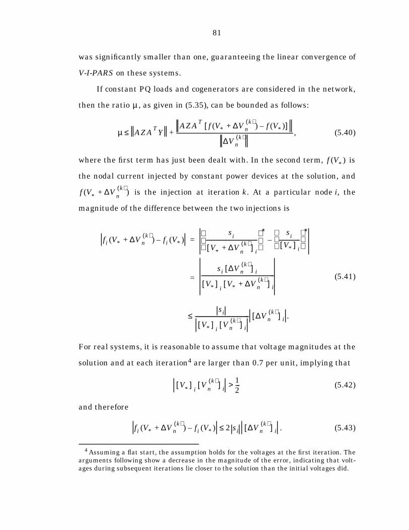
81

was significantly smaller than one, guaranteeing the linear convergence of

V-I-PARS on these systems.

If constant PQ loads and cogenerators are considered in the network,

then the ratio , as given in (5.35), can be bounded as follows:

, (5.40)

where the first term has just been dealt with. In the second term, is

the nodal current injected by constant power devices at the solution, and

is the injection at iteration k. At a particular node i, the

magnitude of the difference between the two injections is

(5.41)

For real systems, it is reasonable to assume that voltage magnitudes at the

solution and at each iteration4 are larger than 0.7 per unit, implying that

(5.42)

and therefore

. (5.43)

4 Assuming a flat start, the assumption holds for the voltages at the first iteration. Thearguments following show a decrease in the magnitude of the error, indicating that volt-ages during subsequent iterations lie closer to the solution than the initial voltages did.

µ

µ AZAT

YAZA

Tf V* ∆Vn

k( )+( ) f V*( )–[ ]

∆Vnk( )

---------------------------------------------------------------------------------------+≤

f V*

( )

f V*

∆Vn

k( )+( )

fi V* ∆Vnk( )

+( ) fi V*( )–s

i

V*

∆Vn

k( )+[ ]

i

-------------------------------------- ∗ s

i

V*[ ]i

--------------- ∗

–

si ∆Vnk( )[ ] i

V*[ ]i

V* ∆Vnk( )

+[ ] i

------------------------------------------------------

si

V*[ ]i

Vnk( )[ ] i

---------------------------------------- ∆Vnk( )[ ] i .≤

=

=

V*

[ ]i

Vn

k( )[ ]i

12--->

fi V* ∆Vnk( )

+( ) fi V*( )– 2 si ∆Vnk( )[ ] i≤

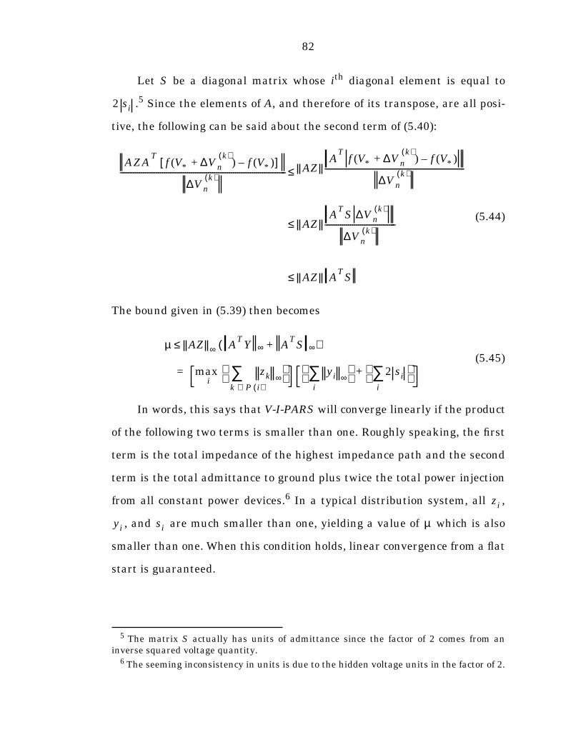
82

Let S be a diagonal matrix whose ith diagonal element is equal to

.5 Since the elements of A, and therefore of its transpose, are all posi-

tive, the following can be said about the second term of (5.40):

(5.44)

The bound given in (5.39) then becomes

(5.45)

In words, this says that V-I-PARS will converge linearly if the product

of the following two terms is smaller than one. Roughly speaking, the first

term is the total impedance of the highest impedance path and the second

term is the total admittance to ground plus twice the total power injection

from all constant power devices.6 In a typical distribution system, all ,

, and are much smaller than one, yielding a value of which is also

smaller than one. When this condition holds, linear convergence from a flat

start is guaranteed.

5 The matrix S actually has units of admittance since the factor of 2 comes from aninverse squared voltage quantity.

6 The seeming inconsistency in units is due to the hidden voltage units in the factor of 2.

2 si

AZAT

f V* ∆Vnk( )

+( ) f V*( )–[ ]

∆Vnk( )--------------------------------------------------------------------------------------- AZ

AT

f V* ∆Vnk( )

+( ) f V*( )–

∆Vnk( )-------------------------------------------------------------------------

AZA

TS ∆Vn

k( )

∆Vnk( )

-------------------------------------

AZ AT

S

≤

≤

≤

µ AZ ∞ AT

Y ∞ AT

S ∞+( )≤

zk ∞k P i( )∈∑

i

max yi ∞i

∑ 2 si

i

∑ +=

zi

yi si µ

83

5.5 Comments

The backward/forward sweep methods presented in this chapter are

applicable to most radial distribution networks. The one modeling limita-

tion is that BFS-PARS cannot handle type 4 ungrounded wye to grounded

wye connected transformers.

Some general observations with regard to the many variations indi-

cate two things. First, the methods based on current generally require less

computation per iteration than their power flow based counterparts. Sec-

ond, the methods which do not update extra variables such as voltage dur-

ing backward sweep and current/power flow during forward sweep, require

less computation per iteration.

Based on these two observations, V-I-PARS appears to be the most

attractive of the BFS-PARS class of algorithms presented, assuming that

the number of iterations required for convergence is comparable among the

various methods. The comparisons of the algorithms are investigated in

more detail in Chapter 8, “Simulation Results”.

It should also be noted that the amount of work per iteration is pro-

portional to the number of buses. Therefore, if the number of iterations

remains constant, the computational complexity increases linearly with

the size of the network, making BFS-PARS suitable for very large radial

distribution systems.

84

Chapter 6

Fast Decoupled Power Flow Algorithms for Radial Systems (DePARS)

One of the most widely used power flow algorithms throughout the

power industry is the fast decoupled Newton method proposed in 1974 in

[26]. This method exploits some of the numerical properties of the standard

power flow formulation to make simplifying assumptions which allow sig-

nificant savings in computation over the standard Newton method. Unfor-

tunately, this approach is not typically suitable for radial distribution

networks. There are often ill-conditioning problems due to the formulation

and, in addition, the assumptions necessary for the simplifications used in

the standard fast decoupled Newton method are often not valid for these

types of systems. Some work, however, has been done to address these

problems [16; 31; 21].

This chapter explores a class of algorithms which exploits the radial

topological structure to reduce the number of equations and unknowns in

the formulation. These algorithms also take advantage of the special

85

numerical structure of the new formulation to further reduce the computa-

tion required for each iteration, in the spirit of the standard fast decoupled

method for meshed transmission systems. This class of algorithms will be

referred to as fast Decoupled Power flow Algorithms for Radial Systems or

DePARS.

This chapter presents four main variants of DePARS. The first of the

four methods, VI-DePARS, is a generalization of the method proposed in

[32] and will be presented in detail. The other variations, one of which is

an extension of the methods proposed in [12], will then be discussed with

respect to VI-DePARS.


The standard fast decoupled methods used in transmission systems

are based on the well-known Newton’s method [28] for solving a non-linear

set of equations. In this case, the non-linear equations being solved are the

power balance equations which specify that, at each bus, the complex

power generated, minus the power absorbed by load, must equal the power

injected into the rest of the network. In a distribution system with one

source bus and many load buses, the traditional power flow formulation

would have six equations for each load bus, balancing the real and reactive

part of the power at each of the three phases.

The traditional fast decoupled method for transmission systems

improves on the standard Newton method, shown in Table 6.1, by making

simplifying approximations which reduce the computational burden for

step 5 and step 6.

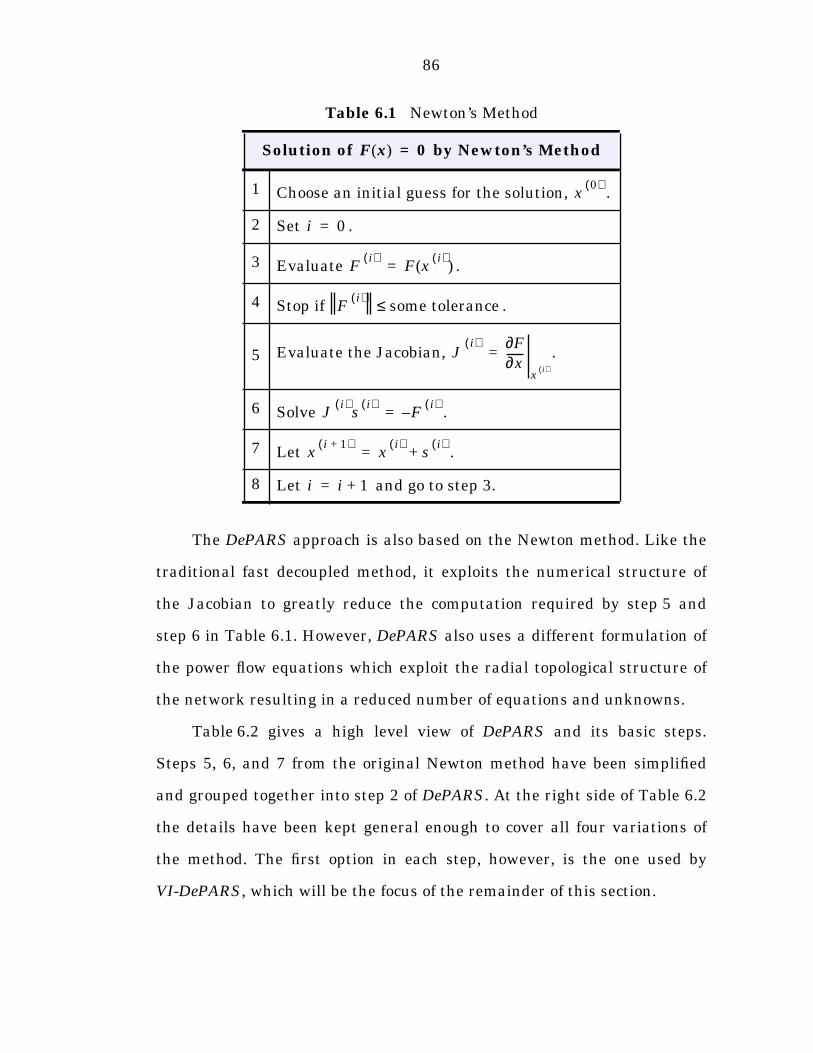
86

The DePARS approach is also based on the Newton method. Like the

traditional fast decoupled method, it exploits the numerical structure of

the Jacobian to greatly reduce the computation required by step 5 and

step 6 in Table 6.1. However, DePARS also uses a different formulation of

the power flow equations which exploit the radial topological structure of

the network resulting in a reduced number of equations and unknowns.

Table 6.2 gives a high level view of DePARS and its basic steps.

Steps 5, 6, and 7 from the original Newton method have been simplified

and grouped together into step 2 of DePARS. At the right side of Table 6.2

the details have been kept general enough to cover all four variations of

the method. The first option in each step, however, is the one used by

VI-DePARS, which will be the focus of the remainder of this section.

Table 6.1 Newton’s Method

Solution of by Newton’s Method

1 Choose an initial guess for the solution, .

2 Set .

3 Evaluate .

4 Stop if .

5 Evaluate the Jacobian, .

6 Solve .

7 Let .

8 Let and go to step 3.

F x( ) 0=

x0( )

i 0=

Fi( )

F xi( )

( )=

Fi( )

some tolerance≤

Ji( )

x∂∂F

xi( )

=

Ji( )

si( )

Fi( )

–=

xi 1+( )

xi( )

si( )

+=

i i 1+=

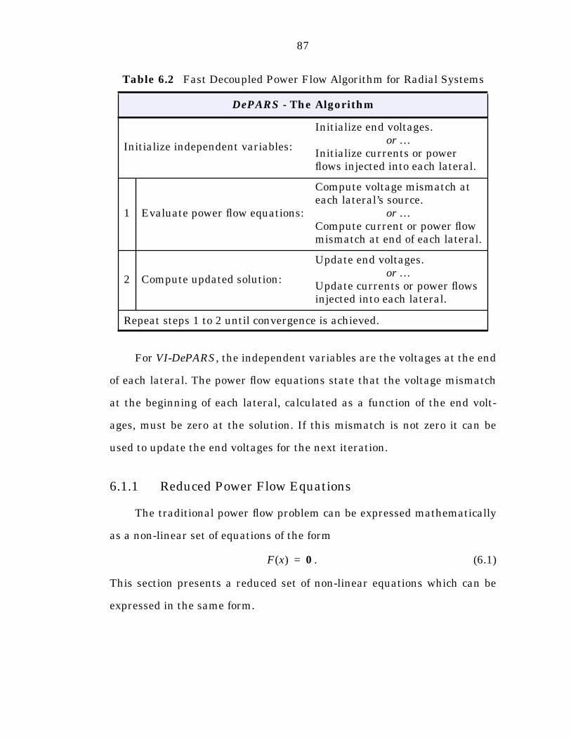
87

For VI-DePARS, the independent variables are the voltages at the end

of each lateral. The power flow equations state that the voltage mismatch

at the beginning of each lateral, calculated as a function of the end volt-

ages, must be zero at the solution. If this mismatch is not zero it can be

used to update the end voltages for the next iteration.

6.1.1 Reduced Power Flow Equations

The traditional power flow problem can be expressed mathematically

as a non-linear set of equations of the form

. (6.1)

This section presents a reduced set of non-linear equations which can be

expressed in the same form.

Table 6.2 Fast Decoupled Power Flow Algorithm for Radial Systems

DePARS - The Algorithm

Initialize independent variables:

Initialize end voltages.or …

Initialize currents or power flows injected into each lateral.

1 Evaluate power flow equations:

Compute voltage mismatch at each lateral’s source.

or …Compute current or power flow mismatch at end of each lateral.

2 Compute updated solution:

Update end voltages.or …

Update currents or power flows injected into each lateral.

Repeat steps 1 to 2 until convergence is achieved.

F x( ) 0=

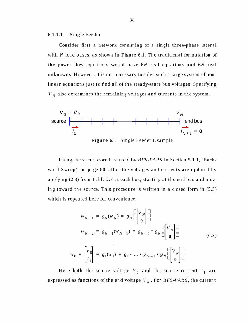
88

6.1.1.1 Single Feeder

Consider first a network consisting of a single three-phase lateral

with N load buses, as shown in Figure 6.1. The traditional formulation of

the power flow equations would have 6N real equations and 6N real

unknowns. However, it is not necessary to solve such a large system of non-

linear equations just to find all of the steady-state bus voltages. Specifying

also determines the remaining voltages and currents in the system.

Using the same procedure used by BFS-PARS in Section 5.1.1, “Back-

ward Sweep”, on page 60, all of the voltages and currents are updated by

applying (2.3) from Table 2.3 at each bus, starting at the end bus and mov-

ing toward the source. This procedure is written in a closed form in (5.3)

which is repeated here for convenience.

(6.2)

Here both the source voltage and the source current are

expressed as functions of the end voltage . For BFS-PARS, the current

Figure 6.1 Single Feeder Example

V N

source

V 0 V 0= V N

I1 IN 1+ 0=

end bus

wN 1– gN wN( ) gNV N

0

= =

wN 2– g

N 1– wN 1–( ) g

N 1– gN

• V N

0

= =

w0

V0

I1

g1 w1( ) g1 …• gN 1– gN••V

N

0

= = =

V0 I1

V N

89

is of primary interest, since it is used during the forward sweep to

update the end voltage . For VI-DePARS, the voltage is of pri-

mary importance, since it is used for mismatch calculation.

At the solution, the difference between the calculated source voltage

and the specified source voltage must be zero. The power flow

equations can therefore be written

. (6.3)

This is a reduced formulation of the power flow problem for a single feeder

which has only three complex equations and three complex unknowns, or

six real equations and six real unknowns. The dimension of this set of non-

linear equations is independent of the number of buses on the lateral and

is a factor of N smaller than the traditional formulation.

6.1.1.2 General Radial Structure

To generalize this formulation to handle an arbitrary radial structure,

first note that the voltage mismatch at the beginning of any lateral can be

computed as a function of the end voltage, as in (6.3), if the currents

injected into each sub-lateral are known. These currents are necessary for

the application of KCL at the branching buses. In a system with L levels of

laterals, the level L laterals have no sub-laterals and can therefore be

updated first. For each lateral and are computed as functions of the

end voltage as follows:

(6.4)

After all level L laterals have been updated, the currents injected into

the sub-laterals of each level lateral are known (the recently cal-

I1 V N( )

V N V0 V N( )

V0 V N( ) V0

F V N( ) V0 V N( ) V0– 0= =

V0 I1

V N

V0

I1

g1 …• gN 1– gN•• V N

0

=

L 1– I1

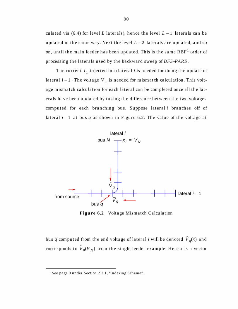
90

culated via (6.4) for level L laterals), hence the level laterals can be

updated in the same way. Next the level laterals are updated, and so

on, until the main feeder has been updated. This is the same RBF1 order of

processing the laterals used by the backward sweep of BFS-PARS.

The current injected into lateral i is needed for doing the update of

lateral . The voltage is needed for mismatch calculation. This volt-

age mismatch calculation for each lateral can be completed once all the lat-

erals have been updated by taking the difference between the two voltages

computed for each branching bus. Suppose lateral i branches off of

lateral at bus q as shown in Figure 6.2. The value of the voltage at

bus q computed from the end voltage of lateral i will be denoted and

corresponds to from the single feeder example. Here x is a vector


Figure 6.2 Voltage Mismatch Calculation

L 1–

L 2–

I1

i 1– V0

i 1–

from source

lateral i

bus qV q

V q

lateral i 1–

x i V N=bus N

Vq x( )

V0 V N( )

91

containing the end voltages of all laterals and denotes the end voltage

for lateral i. These are put into x in RBF1 order.

(6.5)

To compute , it is necessary to use x instead of just since is

affected by the currents injected into the sub-laterals of lateral i and these

currents in turn are functions of the end voltages of the corresponding sub-

laterals. In fact, is a function of the voltages of all end buses supplied

through lateral i, not just of its own end voltage.

The other value of corresponds to the specified source voltage

from the single feeder example and will be denoted . This is the volt-

age at bus q, as computed from the end voltage of lateral . Once again,

the variable x is used since is a function of the voltages of all end buses

supplied through the section of lateral beyond bus q, not just of the

end bus of lateral itself.

Subtracting the two voltages and yields an equation sim-

ilar to (6.3) for lateral i starting at bus q, but is replaced by the vector

x of the end voltages of all laterals.

(6.6)

Note that is not actually constant except when i is the main feeder

and q is the source bus, i.e. the last set of equations when in RBF1 order.

The function does not depend on all elements of x, but only on the volt-

ages of end buses supplied through bus q. This relationship will be seen

xi

V N xi

x

x L ML,( )

x l m,( )

x 1 1,( )

V L ML NL M,, ,( )

V l m N l m,, ,( )

V 1 1 N1 1,, ,( )

= =

Vq V N Vq

Vq

Vq V0

Vq x( )

i 1–

Vq

i 1–

i 1–

Vq x( ) Vq x( )

V N

Fi x( ) Vq x( ) Vq x( )– 0= =

Vq x( )

Fi

92

more clearly in Section 6.1.2.1, “Structure of the System Jacobian”, espe-

cially in Figure 6.3 which illustrates the sparsity structure of the system

Jacobian.

Taking (6.6) for each lateral and combining these equations in RBF1

order,

, (6.7)

yields the new reduced power flow equations which can be expressed com-

pactly as

. (6.8)

Assuming real and imaginary parts are separated, for a system with

M laterals, (6.8) is a set of 6M non-linear equations in 6M real unknowns.

This is also assuming that all buses are three-phase; single and two-phase

laterals would reduce these numbers accordingly.

The reduced power flow equations for VI-DePARS are expressed

mathematically by the non-linear set of equations in (6.8). The evaluation

of these equations is performed by traversing each lateral in RBF1 order,

updating voltages and currents via (6.4), then computing the voltage mis-

matches via (6.6).

F

F L ML,( )

F l m,( )

F 1 1,( )

=

F x( ) 0=

93

6.1.1.3 Class B and Class C Transformers

If lateral i, emanating from bus q on lateral , has a class B or

class C transformer as the incoming branch of bus k,2 the corresponding

equations in (6.4), and consequently in (6.6), may take on a slightly differ-

ent form. For a class B transformer entering bus k, the primary voltage

and current are functions of the of (3.49) which includes , the sum

of the voltages at the primary side of the transformer, not just the two

dimensional secondary voltage . This is described in Section 5.2.1.1,

“Backward Sweep”, on page 66. In this case, the independent variable

associated with lateral i is

. (6.9)

The variable x which contains the end voltages of all laterals will also con-

tain for laterals with class B transformers. This allows (6.6) to still

be used in its present form.

For a lateral with a class C transformer, (6.4) remains unchanged,

although the voltage update formula used is the one in (5.22) which

includes the modified secondary voltage. The mismatch function in (6.6) is

a set of two equations in three unknowns. The additional equation

required to solve the problem is obtained by setting to zero the secondary

side constraint mismatch presented in Section 5.2.2.2, “Backward Sweep”,

as (5.20).

2 Due to the implementation explained in Section 2.2.2.2, “Breadth-First Search”, trans-formers always appear as the first branch on a lateral. So, although the more generalnotation is used here, restricted only to one transformer per lateral, in practice and

.

i 1–

k 1=k 1– q=

wk Vk 1–Σ

Vk

xi

xi

V N

Vk 1–Σ

=

Vk 1–Σ

94

(6.10)

This mismatch is a function of x, since the secondary voltage and current

sums are functions of x. In this case, the function of (6.6), used to

compute the mismatch for lateral i, becomes

. (6.11)

With these small changes in the independent variable and the mis-

match computed for laterals with class B and class C transformers, respec-

tively, the compact form of the reduced power flow equations in (6.8) can

still be used.

6.1.2 Update of Independent Variables

The second step of DePARS, after the evaluation of the power flow

equations, is to update the independent variables, that is, the elements of

x. In the case of VI-DePARS, these are the voltages at the ends of the

laterals.3 In the standard Newton method, this involves the following three

steps:

1. Evaluate the Jacobian at the current solution.

2. Solve a linear system of equations to find the update step.

3. Add the update step to the current solution.

The system Jacobian for the reduced set of power flow equations

in (6.8) is

3 For laterals with class B transformers this also includes , the sum of the voltagesat the primary side of the transformer.

VkΣ

∆ x( ) VkΣ β

k2

yk

------IkΣ′– 0= =

Fi x( )

Fi x( )Vq x( ) Vq x( )–

VkΣ

∆ x( )0= =

V N

Vk 1–Σ

J x( )

95

(6.12)

and has a special numerical structure which can be exploited to greatly

reduce the computation involved in finding a good update step.

6.1.2.1 Structure of the System Jacobian

Since the function F consists of the mismatch functions for each

lateral i, and the variable x is made up of the individual associated with

each lateral i, the system Jacobian can be thought of in terms of block ele-

ments associated with a pair of laterals. The block element , in

block row i and block column j, is the sensitivity of the mismatch at

lateral i to changes in the independent variables corresponding to lateral j.

First consider a single feeder system where the mismatch function is

as given in (6.3). The Jacobian for this simple system is just a single

block element and can be expressed using the chain rule and the branch

Jacobians. The branch Jacobian for bus k’s incoming branch is the

Jacobian of the branch update equation in (2.3) from Table 2.3. This

branch update function is

(6.13)

and therefore the branch Jacobian is

. (6.14)

The system Jacobian for this simple single feeder case gives the sensi-

tivity of the calculated source voltage mismatch to variations in the end

J x( )x∂

∂F=

Fi

xi

Fi∂ x j∂⁄

F V N( )

Gk

wk 1– gk wk( )=

Gk wk∂∂gk Vk∂

∂Vk 1–

Ik 1+∂∂Vk 1–

Vk∂∂Ik

Ik 1+∂∂Ik

= =

96

voltage. It can be written, using the chain rule, as the product of the

branch Jacobians from the source bus to the end bus

, (6.15)

where the first term in the product is just the upper half of and the last

term is the left half of .

Extending this to the general radial structure, each block element of

the system Jacobian can be expressed, using the chain rule, as a product of

branch Jacobians along the path between the supplying bus of lateral i and

the end bus of lateral j. If lateral i branches off from its parent lateral at

bus q and the end bus of lateral j is bus n, then changes in at bus n can

only affect the mismatch at bus q if bus n is supplied through bus q. In

other words, if bus q does not lie on the path between bus n and the source,

then . This determines the sparsity structure of the system

Jacobian .

If bus q does lie on the path between bus n and the source, then the

corresponding block element is non-zero and fits into one of the

four categories listed in Table 6.3. In order to simplify the presentation, the

equations given in Table 6.3 are for the case with no class B or class C

transformers present.

The first type of non-zero blocks are those on the block diagonal of the

system Jacobian. These diagonal blocks are formed via (6.16) in a manner

analogous to the single feeder case in (6.15). The second type is the set of

non-zero blocks above the diagonal and is similar to the first except that

refers to the bus following bus q on lateral j, hence it is that is

affected instead of . For non-zero blocks of type 3 and type 4, let bus p

J VN

( )V

N∂∂F

VN

∂∂V0

w1∂∂V0 G

2… G

N 1– V N∂∂gN⋅ ⋅ ⋅ ⋅= = =

G1

GN

x j

Fi

Fi∂ x j∂⁄ 0=

J x( )

Fi∂ x j∂⁄

q 1+ Vq

Vq

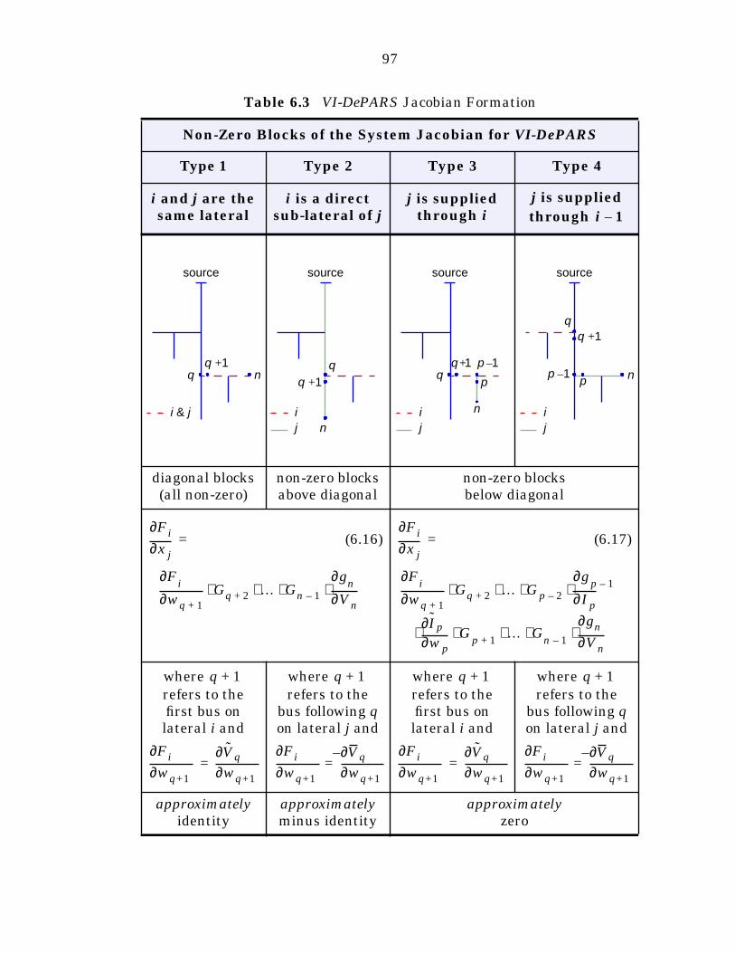
97

Table 6.3 VI-DePARS Jacobian Formation

Non-Zero Blocks of the System Jacobian for VI-DePARS

Type 1 Type 2 Type 3 Type 4

i and j are the same lateral

i is a direct sub-lateral of j

j is supplied through i

j is supplied through

diagonal blocks(all non-zero)

non-zero blocks above diagonal

non-zero blocksbelow diagonal

(6.16) (6.17)

where refers to the first bus on lateral i and

where refers to the

bus following q on lateral j and

where refers to the first bus on lateral i and

where refers to the

bus following q on lateral j and

approximately identity

approximately minus identity

approximatelyzero

i 1–

i & j

source

q nq 1+

q 1+

source

q

n

i

j

source

n

p

p 1–

i

j

qq 1+

source

q

npp 1–

i

j

q 1+

x j∂∂Fi =

wq 1+∂∂F

i Gq 2+ … Gn 1– Vn∂∂g

n⋅ ⋅ ⋅ ⋅

x j∂∂Fi =

wq 1+∂∂F

i Gq 2+ … Gp 2– I p∂∂g

p 1–

wp∂∂I p G

p 1+ … Gn 1– Vn∂

∂gn

⋅ ⋅ ⋅ ⋅

⋅ ⋅ ⋅ ⋅ ⋅

q 1+

wq 1+∂∂Fi

wq 1+∂∂Vq=

q 1+

wq 1+∂∂Fi

wq 1+∂∂Vq–

=

q 1+

wq 1+∂∂Fi

wq 1+∂∂Vq=

q 1+

wq 1+∂∂Fi

wq 1+∂∂Vq–

=

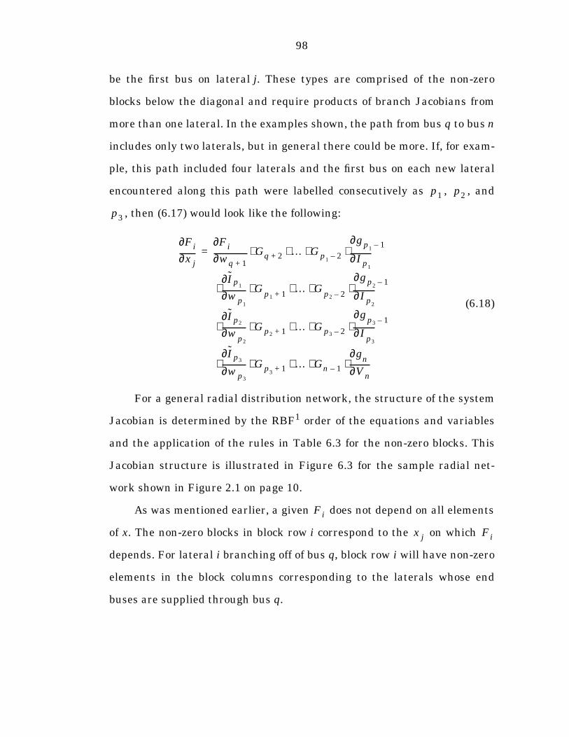
98

be the first bus on lateral j. These types are comprised of the non-zero

blocks below the diagonal and require products of branch Jacobians from

more than one lateral. In the examples shown, the path from bus q to bus n

includes only two laterals, but in general there could be more. If, for exam-

ple, this path included four laterals and the first bus on each new lateral

encountered along this path were labelled consecutively as , , and

, then (6.17) would look like the following:

(6.18)

For a general radial distribution network, the structure of the system

Jacobian is determined by the RBF1 order of the equations and variables

and the application of the rules in Table 6.3 for the non-zero blocks. This

Jacobian structure is illustrated in Figure 6.3 for the sample radial net-

work shown in Figure 2.1 on page 10.

As was mentioned earlier, a given does not depend on all elements

of x. The non-zero blocks in block row i correspond to the on which

depends. For lateral i branching off of bus q, block row i will have non-zero

elements in the block columns corresponding to the laterals whose end

buses are supplied through bus q.

p1 p2

p3

x j∂∂Fi

wq 1+∂∂Fi Gq 2+ … Gp1 2– I p1

∂

∂gp1 1–

wp1∂∂I p1 G

p1 1+ … Gp2 2– I p2

∂

∂gp2 1–

wp2

∂∂I p2 Gp2 1+ … Gp3 2– I

p3∂

∂gp3 1–

wp3∂∂I p3 Gp3 1+ … Gn 1– Vn∂

∂gn

⋅ ⋅ ⋅ ⋅

⋅ ⋅ ⋅ ⋅ ⋅

⋅ ⋅ ⋅ ⋅ ⋅

⋅ ⋅ ⋅ ⋅ ⋅

=

Fi

x j Fi

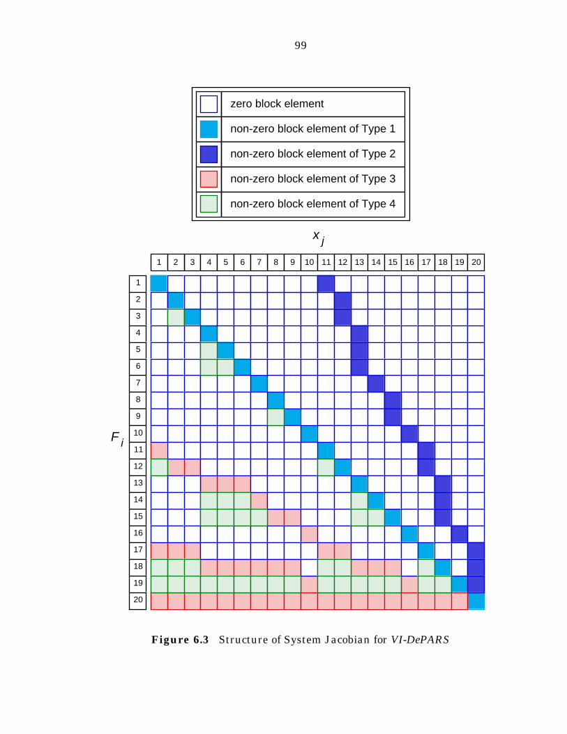
99

Figure 6.3 Structure of System Jacobian for VI-DePARS

1 32 4 5 6 87 9 10 11 1312 14 15 16 1817 19 20

1

2

3

4

5

6

7

8

9

10

11

12

13

14

15

16

17

18

19

20

non-zero block element of Type 2


zero block element



x j

F i

100

6.1.2.2 Numerical Properties of the System Jacobian

The process of building the system Jacobian requires the application

of (6.16) or (6.17) for each non-zero block as determined by the topology of

the network. Each non-zero block is a product of branch Jacobians which

must be evaluated first. The branch Jacobian of (6.14) relates the sen-

sitivity of voltages and currents at bus to small variations in the volt-

ages and currents at bus k. For a three-phase branch, it is typically a

12 x 12 real matrix.4 Even for a very simple distribution line represented

with the standard π-model, each element of the matrix is a very complex

expression depending not only on the parameters of the line but also on

any load, shunt capacitor, or cogenerator at bus k. For a transformer the

expression can be even more complicated.

To include in a computer program an analytical expression for each of

the 144 terms of each variation of the branch Jacobian is not practical due

to the number of different expressions and their extreme complexity. The

building of the true system Jacobian via products of true branch Jacobians

is therefore not a viable option either. Some numerical approximation is

needed.

In order to determine the numerical structure of the system Jacobian

it is necessary to first examine carefully the numerical properties of the

branch Jacobians for each type of branch. Deriving an analytical expres-

sion for each element and analyzing it to determine which terms can be

neglected and what approximations can be made would also be prohibi-

4 If one or both sides of the branch are in an ungrounded section of the network, thisdimension is reduced to 10 x 10 or 8 x 8, respectively. Note that it is necessary to separateeach complex variable into two real variables in order to differentiate to find the truebranch Jacobian.

Gk

k 1–

101

tively tedious. However, some reasonable approximations can be made by

examining the relative magnitudes of certain quantities when expressed in

per unit.

For the incoming branch of bus k, the branch Jacobian contains

the sensitivities of and to small changes in and . Sup-

pose this branch is a switch, modeled as a zero impedance connection. In

this case, small changes in cause identical changes in and small

changes in cause identical changes in . In other words, the diago-

nal blocks of are identity blocks. The off-diagonal block based on the

sensitivity of to is a zero block since changes in have no

effect on the voltage . The other off-diagonal block is nearly zero as

well, under the assumption that the admittances and power injections of

loads, shunt capacitors, and cogenerators are small relative to voltage

magnitudes when expressed in per unit. From the KCL equation in (5.2) it

can be seen that does have a small effect on the currents injected by

loads, shunt capacitors, and cogenerators. However, assuming the admit-

tance or power parameters are small with respect to voltage, the sensitiv-

ity of , and therefore of also, to can be neglected. This is

equivalent to approximating loads, shunt capacitors, and cogenerators by

their corresponding current injections. For a switch, then, the branch Jaco-

bian can be approximated by the appropriately sized identity matrix.5

Using I to denote an identity block

. (6.19)

5 When using this approximation, it is not necessary to split up complex variables intotwo real variables. Hence, for a three-phase branch in a grounded section of the network

is a 6 x 6 identity matrix.

Gk

Vk 1– Ik Vk Ik 1+

Vk Vk 1–

Ik 1+ Ik

Gk

Vk 1– Ik 1+ Ik 1+

Vk 1–

Vk

Ik′ Ik Vk

Gk

Gk

GkI 0

0 I≈

102

If bus k’s incoming branch is a distribution line modeled as described

in Section 3.4, “Distribution Line Model”, then the numerical properties of

(3.19) and (3.20) from Table 3.6 must be examined in order to derive an

approximation for . For practical distribution lines the elements of the

line impedance matrix and the line charging admittance matrix are

typically small with respect to voltage magnitudes when expressed in per

unit. When differentiating, under this assumption, the last term of (3.19)

and the first term of (3.20) can be neglected. This is equivalent to approxi-

mating the distribution line as a zero impedance branch with no charging.

As with the switch, this implies that the branch Jacobian can be

approximated by the appropriately sized identity matrix.5

In a system with only lines and switches but no transformers, each

branch Jacobian can be approximated by an identity matrix. Voltages and

currents are essentially decoupled from one another. It is important to note

that these approximations are only for simplifying the Jacobian used to

compute the update step in Newton’s method. They have no effect on the

final solution, which is still based on the full models described in

Chapter 3, “Detailed Component Models”.

The diagonal blocks of the system Jacobian are under type 1 in

Table 6.3 and are formed via (6.16). Using the identity approximations for

the branch Jacobians yields an identity block in the system Jacobian as

well.

(6.20)

Gk

Zk Yk

Gk

x j∂∂Fi

I 0I 0

0 I… I 0

0 I

I

0⋅ ⋅ ⋅ ⋅≈

I=

103

Type 2 non-zero blocks, those above the diagonal, are formed by the

same equation except that the first term has a negative sign, resulting in a

negative identity block in the system Jacobian.

(6.21)

Using the identity approximation to the branch Jacobian in (6.17) for

type 3 non-zero blocks yields

(6.22)

Here the result is a zero block in the system Jacobian. This is due to the

fact that the only coupling between the voltages involved is through the

current , but the approximation decouples voltages and currents. The

only difference for type 4 non-zero blocks is a leading negative sign. These

blocks can therefore also be approximated by zero. The last row of

Table 6.3 summarizes these approximations.

6.1.2.3 Transformers

Building non-zero blocks of the system Jacobian which involve trans-

formers is somewhat more complicated. First, note that there can be no

transformers on the relevant part of lateral j for a type 2 non-zero block, so

the approximations for these blocks are never affected by transformers.

x j∂∂Fi

I 0– I 0

0 I… I 0

0 I

I

0⋅ ⋅ ⋅ ⋅≈

I–=

x j∂∂Fi

I 0I 0

0 I… I 0

0 I

0

I0 I

I 0

0 I… I 0

0 I

I

0⋅ ⋅ ⋅ ⋅ ⋅ ⋅ ⋅ ⋅ ⋅≈

I 00

I0 I

I

0⋅ ⋅ ⋅

0

=

=

I p

104

Second, note that if a transformer is approximated by its ideal equiva-

lent with no leakage admittance, then currents are completely decoupled

from voltages and vice versa. Changes in secondary voltage have no effect

on primary current and changes in secondary current have no effect on pri-

mary voltage. This means that the off-diagonal blocks of can be approx-

imated by a zero block for a transformer.

Given that a transformer always appears as the first branch on the

lateral,6 the lower right block of is not even used in the formation of the

system Jacobian for type 1 blocks since the first term of (6.16) includes

only the left half of . The same is true about the first term of (6.17) for

type 3 and type 4 blocks. In fact, for a network with a transformer entering

bus p, the identity approximations for the lines and switches disappear

and (6.17) becomes

(6.23)

Even without knowing the value of these sub-diagonal blocks

can still be approximated by zero. This means that it is not necessary to

evaluate the lower right block of for a transformer since it is never used

in the formation of the approximated system Jacobian.

The only non-zero blocks of the approximated system Jacobian

affected by transformers are the type 1 diagonal blocks. Suppose bus k7 is

the first bus on lateral i and its incoming branch is a transformer. The

6 See Section 2.2.2.2, “Breadth-First Search”.7 Here k is also equal to in the figure for type 1 blocks in Table 6.3.

Gk

Gk

Gk

x j∂∂Fi

I 00

I0

I p 1+∂∂I p

I

0⋅ ⋅ ⋅≈

0 .=

I p∂ I p 1+∂⁄

Gk

q 1+

105

diagonal element in block row i can be approximated by the upper left

block element of .

(6.24)

This relationship between secondary and primary voltages, however,

depends on the connection type. For class A transformers, this partial

derivative is computed from (3.39) of Table 3.9 and yields

. (6.25)

For class B transformers, is a function of as well as . Differen-

tiating (3.52) of Table 3.10 gives the relevant expression:

(6.26)

For class C transformers, the corresponding block diagonal element of the

approximated Jacobian consists of the partial derivatives of (5.22) and

(6.10).

(6.27)

Table 6.4 shows, for each transformer type, the constant matrix

depending only on and which results from the evaluation of (6.25),

Gk

x j∂∂Fi

Vk∂∂Vk 1–

0I 0

0 I… I 0

0 I

I

0⋅ ⋅ ⋅ ⋅≈

Vk∂∂Vk 1–=

xi

∂∂Fi

Vk

∂∂Vk 1–≈ Yk

sp( )

1–Yk

ss–=

gk Vk 1–Σ

Vk

xi∂∂Fi

Vk∂∂Vk 1–

Vk 1–Σ

∂

∂Vk 1–

≈Yk

sp

1 1 1

1– 0Yk

ss–

0

0 0 1

=

xi

∂∂Fi Vk∂

∂Vk 1–

Vk∂∂Vk

Σ

≈Yk

spYk

ss 13---

2 1– 1–

1– 2 1–1– 1– 2

⋅

\–

1 1 1

=

αk βk

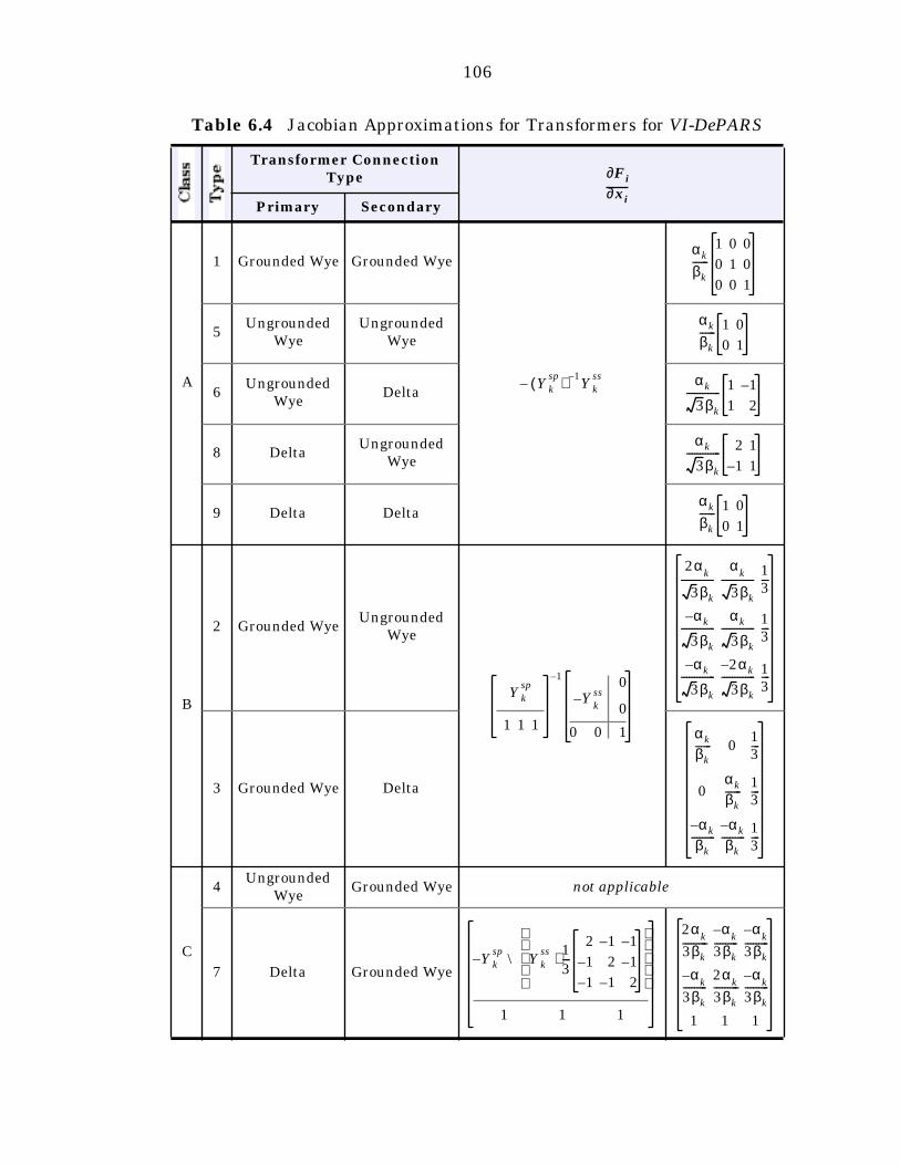
106

Table 6.4 Jacobian Approximations for Transformers for VI-DePARS


Primary Secondary

A

1 Grounded Wye Grounded Wye

5Ungrounded

WyeUngrounded

Wye

6Ungrounded

WyeDelta

8 DeltaUngrounded

Wye

9 Delta Delta

B

2 Grounded WyeUngrounded

Wye

3 Grounded Wye Delta

C

4Ungrounded

WyeGrounded Wye not applicable

7 Delta Grounded Wye

xi∂∂Fi

Yksp( ) 1–

Ykss

–

αk

βk

------1 0 0

0 1 0

0 0 1

αk

βk

------ 1 0

0 1

αk

3βk

------------- 1 1–

1 2

αk

3βk

------------- 2 1

1– 1

αk

βk

------ 1 0

0 1

Yksp

1 1 1

1– 0Y

kss–

0

0 0 1

2αk

3βk

-------------α

k

3βk

-------------13---

αk–

3βk

-------------αk

3βk

-------------13---

αk–

3βk

-------------2αk–

3βk

------------- 13---

αk

βk------ 0

13---

0αk

βk------

13---

αk–

βk---------

αk–

βk---------

13---

Yksp

Ykss 1

3---

2 1– 1–

1– 2 1–

1– 1– 2

⋅

\–

1 1 1

2αk

3βk----------

αk

–

3βk---------

αk

–

3βk---------

αk

–

3βk

---------2α

k

3βk

----------α

k–

3βk

---------

1 1 1

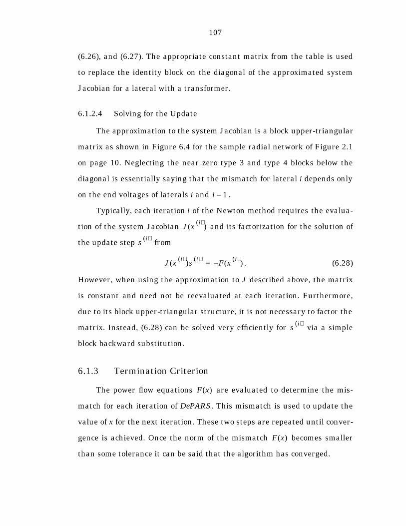
107

(6.26), and (6.27). The appropriate constant matrix from the table is used

to replace the identity block on the diagonal of the approximated system

Jacobian for a lateral with a transformer.

6.1.2.4 Solving for the Update

The approximation to the system Jacobian is a block upper-triangular

matrix as shown in Figure 6.4 for the sample radial network of Figure 2.1

on page 10. Neglecting the near zero type 3 and type 4 blocks below the

diagonal is essentially saying that the mismatch for lateral i depends only

on the end voltages of laterals i and .

Typically, each iteration i of the Newton method requires the evalua-

tion of the system Jacobian and its factorization for the solution of

the update step from

. (6.28)

However, when using the approximation to J described above, the matrix

is constant and need not be reevaluated at each iteration. Furthermore,

due to its block upper-triangular structure, it is not necessary to factor the

matrix. Instead, (6.28) can be solved very efficiently for via a simple

block backward substitution.


The power flow equations are evaluated to determine the mis-

match for each iteration of DePARS. This mismatch is used to update the

value of x for the next iteration. These two steps are repeated until conver-

gence is achieved. Once the norm of the mismatch becomes smaller

than some tolerance it can be said that the algorithm has converged.

i 1–

J xi( )

( )

si( )

J xi( )

( )si( )

F xi( )

( )–=

si( )

F x( )

F x( )

108

Figure 6.4 Approximation to the System Jacobian for VI-DePARS

1 32 4 5 6 87 9 10 11 1312 14 15 16 1817 19 20

1

2

3

4

5

6

7

8

9

10

11

12

13

14

15

16

17

18

19

20

negative identity blocks

identity block (or from Table 6.4)

zero block element

x j

F i

109

It is also possible to use the termination criterion used for the net-

work reduction methods of Chapter 4. This approach requires that the

norm of the difference in bus voltages between iterations be smaller than a

given tolerance.

6.2 Implementation

In many respects DePARS is very similar to the backward/forward

sweep methods of Chapter 5. The function evaluation for VI-DePARS in

the implementation is, in fact, the same routine as the one used for back-

ward sweep in VI-VI-PARS and V-VI-PARS. In the fast decoupled method,

the end voltages are updated directly via an approximate Newton step as

opposed to the complete forward sweep used in the backward/forward

sweep methods.

Because of the simple structure of the approximated Jacobian, it is

not even necessary to explicitly form the matrix. Once the mismatches

have been calculated, the update step for each lateral can be computed

directly as

(6.29)

for laterals without transformers, and

(6.30)

for laterals with transformers. Here refers to the update step for

lateral , the parent of lateral i. The calculation of the update steps

must therefore proceed in BF8 order, starting with the main feeder. The


Fi

si si 1– Fi–=

si xi∂∂F

i

1–

si 1– Fi–( )=

si 1–

i 1–

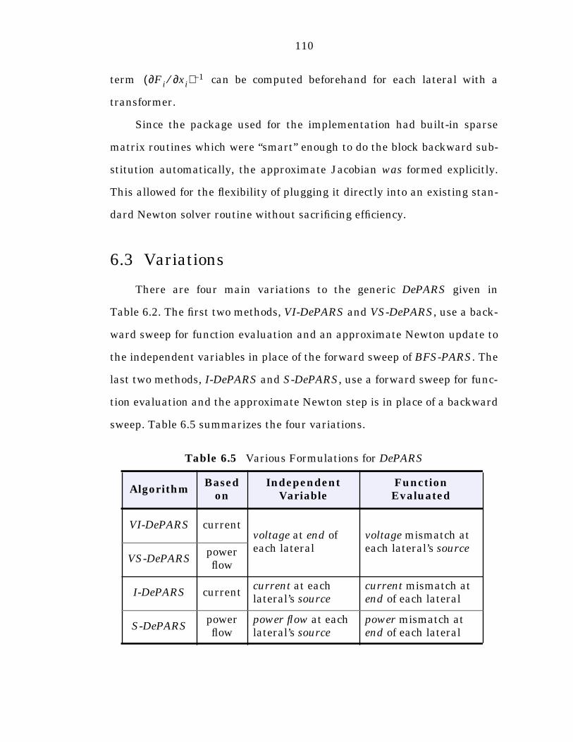
110

term can be computed beforehand for each lateral with a

transformer.

Since the package used for the implementation had built-in sparse

matrix routines which were “smart” enough to do the block backward sub-

stitution automatically, the approximate Jacobian was formed explicitly.

This allowed for the flexibility of plugging it directly into an existing stan-

dard Newton solver routine without sacrificing efficiency.

6.3 Variations

There are four main variations to the generic DePARS given in

Table 6.2. The first two methods, VI-DePARS and VS-DePARS, use a back-

ward sweep for function evaluation and an approximate Newton update to

the independent variables in place of the forward sweep of BFS-PARS. The

last two methods, I-DePARS and S-DePARS, use a forward sweep for func-

tion evaluation and the approximate Newton step is in place of a backward

sweep. Table 6.5 summarizes the four variations.

Table 6.5 Various Formulations for DePARS

AlgorithmBased

onIndependent

VariableFunction Evaluated

VI-DePARS currentvoltage at end of each lateral

voltage mismatch at each lateral’s source

VS-DePARSpower flow

I-DePARS currentcurrent at each lateral’s source

current mismatch at end of each lateral

S-DePARSpower flow

power flow at each lateral’s source

power mismatch at end of each lateral

Fi∂ xi∂⁄( ) 1–

111

6.3.1 VI-DePARS

VI-DePARS is the variation presented in detail in Section 6.1,

“Detailed Solution Algorithm”. It computes voltage mismatches at the

beginning of each lateral as a function of the end voltages and is based on

current as opposed to power flow. This is the algorithm presented in [32]

for networks which have only type 1 grounded wye to grounded wye trans-

formers.

The approach proposed in [17] is based on a similar idea. For a system

consisting of a single feeder, it is equivalent to VI-DePARS, using (6.29) to

update the end voltages directly from the voltage mismatch at the source.

However, in the extension to a general radial structure, instead of updat-

ing the end voltage of all laterals at each iteration, the equations associ-

ated with each lateral are solved one by one to completion. Once

convergence is achieved for all level l laterals, the level are solved.

When all the laterals have been solved the process is repeated. This nested

looping, of course, is inefficient and, fortunately, not necessary, as has been

shown.

6.3.2 VS-DePARS

VS-DePARS is the power flow based counterpart to VI-DePARS. It

uses the same independent variables and the mismatches computed are

still the voltage mismatches at the beginning of each lateral. The function

evaluation, however, is based on the backward sweep used by VS-VS-PARS

described in Section 5.3.2.9 Many of the differences between VI-VI-PARS

9 This backward sweep is also used by V-VS-PARS of Section 5.3.4.

l 1–

112

and VS-VS-PARS described in this section are also relevant to the differ-

ences between VI-DePARS and VS-DePARS.

Since this method computes the same mismatch as a function of the

same variables, the same approximate Jacobian can be used. An extensive

analysis of the branch Jacobians, now based on from (2.5), lead to the

same approximations yielding the same approximate system Jacobian.

6.3.3 I-DePARS

In the single feeder example of Figure 6.1, there are two boundary

conditions: the source voltage is a specified constant and the end current is

zero. The first two variations of DePARS are based on using the boundary

condition at the end of the lateral to compute backward toward the source,

obtaining a voltage mismatch at the source as a function of the end volt-

age. I-DePARS takes the opposite approach. The source voltage boundary

condition is used to calculate in the forward direction to obtain a current

mismatch at the end of the lateral as a function of the current injected at

the source.

In this case, the independent variables are the currents injected into

the beginning of each lateral. The function evaluation is equivalent to a

forward sweep and the approximate Newton update of the independent

variables is in place of a backward sweep. In fact, the routine used to do

the function evaluation is the same as the one used for the forward sweep

of VI-VI-PARS and VI-I-PARS, which is described in detail in Section 5.1.2,

“Forward Sweep”.

hk

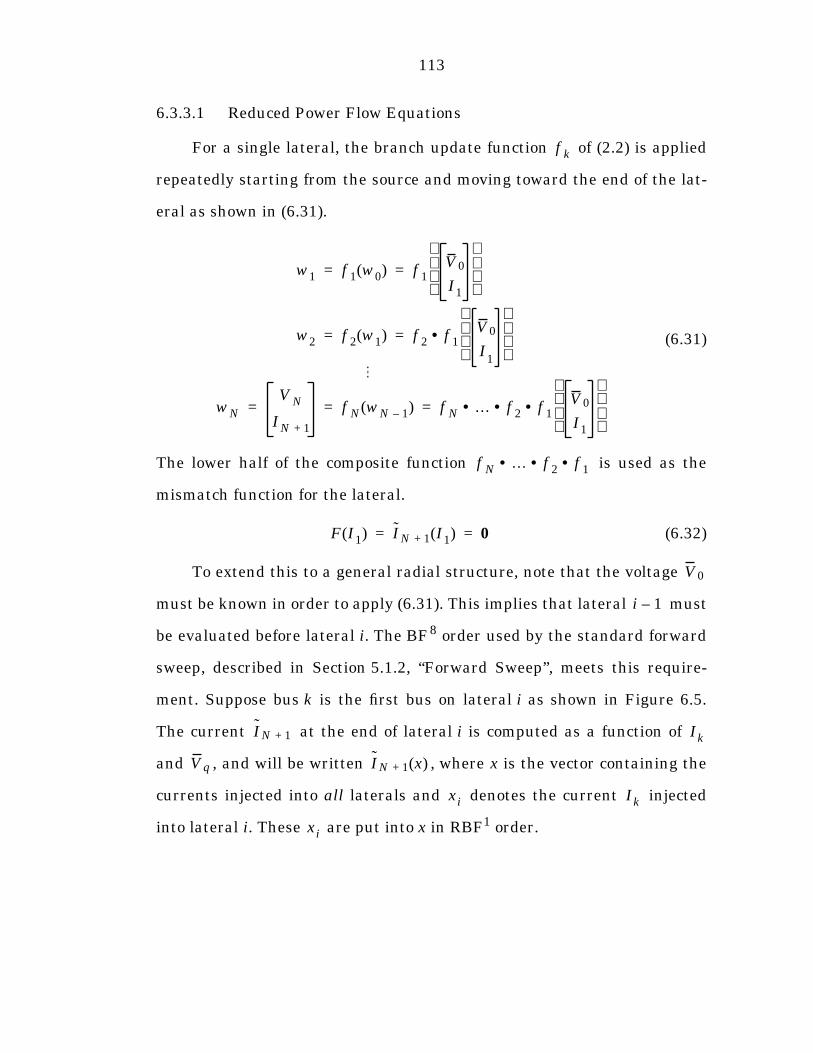
113

6.3.3.1 Reduced Power Flow Equations

For a single lateral, the branch update function of (2.2) is applied

repeatedly starting from the source and moving toward the end of the lat-

eral as shown in (6.31).

(6.31)

The lower half of the composite function is used as the

mismatch function for the lateral.

(6.32)

To extend this to a general radial structure, note that the voltage

must be known in order to apply (6.31). This implies that lateral must

be evaluated before lateral i. The BF8 order used by the standard forward

sweep, described in Section 5.1.2, “Forward Sweep”, meets this require-

ment. Suppose bus k is the first bus on lateral i as shown in Figure 6.5.

The current at the end of lateral i is computed as a function of

and , and will be written , where x is the vector containing the

currents injected into all laterals and denotes the current injected

into lateral i. These are put into x in RBF1 order.

f k

w1 f 1 w0( ) f 1V0

I1

= =

w2 f 2 w1( ) f 2 f 1• V0

I1

= =

wN

V N

IN 1+

f N wN 1–( ) f N …• f 2 f 1•• V0

I1

= = =

f N …• f 2 f 1••

F I1( ) IN 1+ I1( ) 0= =

V0

i 1–

IN 1+ Ik

Vq IN 1+ x( )

xi Ik

xi

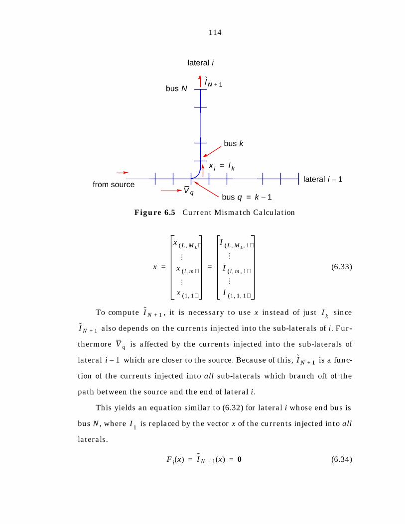
114

(6.33)

To compute , it is necessary to use x instead of just since

also depends on the currents injected into the sub-laterals of i. Fur-

thermore is affected by the currents injected into the sub-laterals of

lateral which are closer to the source. Because of this, is a func-

tion of the currents injected into all sub-laterals which branch off of the

path between the source and the end of lateral i.

This yields an equation similar to (6.32) for lateral i whose end bus is

bus N, where is replaced by the vector x of the currents injected into all

laterals.

(6.34)

Figure 6.5 Current Mismatch Calculation

from source

lateral i

bus k

V q

lateral i 1–

x i Ik=

bus NIN 1+

bus q k 1–=

x

x L ML,( )

x l m,( )

x 1 1,( )

I L ML 1, ,( )

I l m 1, ,( )

I 1 1 1, ,( )

= =

IN 1+ Ik

IN 1+

Vq

i 1– IN 1+

I1

Fi x( ) IN 1+ x( ) 0= =

115

Taking (6.34) for each lateral and combining these equations in RBF1 order

as in (6.7) yields the new reduced power flow equations which can be still

be expressed compactly as

. (6.35)

Note that the implementation of (6.35) in this case requires that the later-

als be evaluated in BF8 order, not in the order they appear in F and x.10

As with VI-DePARS, a class B or class C transformer entering bus k

causes the variables or mismatch functions for lateral i to change slightly

from the standard and . For a lateral with a class B transformer,

the voltage update formula used is the one in (5.15) which includes the

modified primary current. The mismatch function in (6.34) is a set of two

equations in three unknowns. The additional equation required to solve

the problem is obtained by setting to zero the primary side constraint mis-

match presented in Section 5.2.1.2, “Forward Sweep”, as (5.12) or (5.13).

For type 2 grounded wye to ungrounded wye transformers, (5.12) gives

(6.36)

and for type 3 grounded wye to delta transformers, (5.13) gives

. (6.37)

This mismatch is a function of x since the primary voltage and current

sums are functions of x. In this case, the mismatch function becomes

. (6.38)

10 The ordering of F and x need only satisfy the constraint that they be sorted by laterallevel. RBF order was chosen primarily for consistency with VI-DePARS.

F x( ) 0=

Ik IN 1+

IkΣ

∆ x( ) IkΣ

0= =

IkΣ

∆ x( ) IkΣ yk

αk2

------Vk 1–Σ

– 0= =

Fi x( )

Fi

x( )IN 1+ x( )

IkΣ

∆ x( )

0= =

116

For a class C transformer entering bus k, the secondary voltage and

current are functions of the of (3.60) which includes , the sum of

the currents at the secondary side of the transformer, not just the two

dimensional primary current . This is described in Section 5.2.2.1, “For-

ward Sweep”, on page 69. In this case, the independent variable associ-

ated with lateral i is

. (6.39)

The variable x, which contains the currents injected into all laterals, will

also contain for laterals with class C transformers. This allows (6.34) to

be used in its present form.

With these small changes in the mismatch and the independent vari-

able for laterals with class B and class C transformers, respectively, the

compact form of the reduced power flow equations in (6.35) can still be

used.

6.3.3.2 Update of the Independent Variables

As with the formulation for VI-DePARS, the elements of the system

Jacobian can be formed via the chain rule as the product of branch Jacobi-

ans. The branch Jacobian for I-DePARS is the Jacobian of the branch

update function in (2.2) from Table 2.3. This branch update function is

(6.40)

and the branch Jacobian is therefore

wk 1– IkΣ′

Ik

xi

xi

Ik

IkΣ′

=

IkΣ′

Gk

wk f k wk 1–( )=

117

. (6.41)

Suppose lateral j branches off of its parent at bus q and lateral i’s end

bus is bus n.11 If bus q does not lie on the path from the source to bus n,

then the corresponding block element of the system Jacobian is a

zero block. If bus q does lie on the path from the source to bus n, then the

corresponding block is non-zero. Table 6.6 summarizes the formation of the

non-zero blocks of the system Jacobian. In order to simplify the presenta-

tion, the equations given in Table 6.6 are for the case with no class B or

class C transformers present. This leads to the structure shown in

Figure 6.6 for the sample radial network shown in Figure 2.1 on page 10.

This structure is the transpose of the Jacobian structure for VI-DePARS

shown in Figure 6.3.

For lines and switches, the branch Jacobian in (6.41) can once again

be approximated by an identity matrix, under the same assumptions about

the relative magnitudes of per unit circuit parameters and per unit volt-

ages. Following a development similar to that of Section 6.1.2.2, “Numeri-

cal Properties of the System Jacobian”, and Section 6.1.2.3,

“Transformers”, leads to similar approximations. The type 3 and type 4

blocks, now above the diagonal, are approximated by zero, the type 2

blocks below the diagonal are approximated by negative identity, and the

diagonal type 1 blocks, except when dealing with transformers, are approx-

imated by identity blocks.

11 Here i and j are exchanged from the scenario used in Table 6.3.

Gk wk 1–∂∂f k Vk 1–∂

∂Vk

Ik∂∂Vk

Vk 1–∂∂Ik 1+

Ik∂∂Ik 1+

= =

Fi

∂ xj

∂⁄

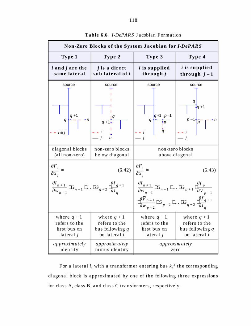
118

For a lateral i, with a transformer entering bus k,2 the corresponding

diagonal block is approximated by one of the following three expressions

for class A, class B, and class C transformers, respectively.

Table 6.6 I-DePARS Jacobian Formation

Non-Zero Blocks of the System Jacobian for I-DePARS

Type 1 Type 2 Type 3 Type 4

i and j are the same lateral

j is a direct sub-lateral of i

i is supplied through j

i is supplied through

diagonal blocks(all non-zero)

non-zero blocks below diagonal

non-zero blocksabove diagonal

(6.42) (6.43)

where refers to the first bus on

lateral j

where refers to the

bus following q on lateral i

where refers to the first bus on

lateral j

where refers to the

bus following q on lateral i

approximately identity

approximately minus identity

approximatelyzero

j 1–

i & j

source

q nq 1+

q 1+

source

q

n

i

j

source

n

p

p 1–

i

j

qq 1+

source

q

npp 1–

i

j

q 1+

x j∂∂Fi =

wn 1–∂∂I

n 1+ Gn 1– … Gq 2+ Iq∂∂f

q 1+⋅ ⋅ ⋅ ⋅

x j∂∂Fi =

wn 1–∂∂I

n 1+ Gn 1– … Gp 1+ V p 1–∂∂f

p

wp 2–∂∂V p 1– G

p 2– … Gq 2+ Iq∂

∂f q 1+

⋅ ⋅ ⋅ ⋅

⋅ ⋅ ⋅ ⋅ ⋅

q 1+ q 1+ q 1+ q 1+

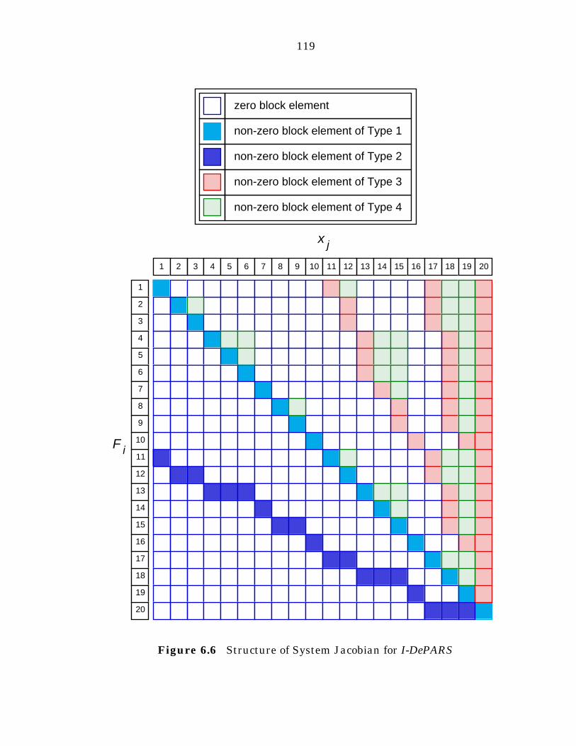
119

Figure 6.6 Structure of System Jacobian for I-DePARS

1 32 4 5 6 87 9 10 11 1312 14 15 16 1817 19 20

1

2

3

4

5

6

7

8

9

10

11

12

13

14

15

16

17

18

19

20



zero block element



x j

F i

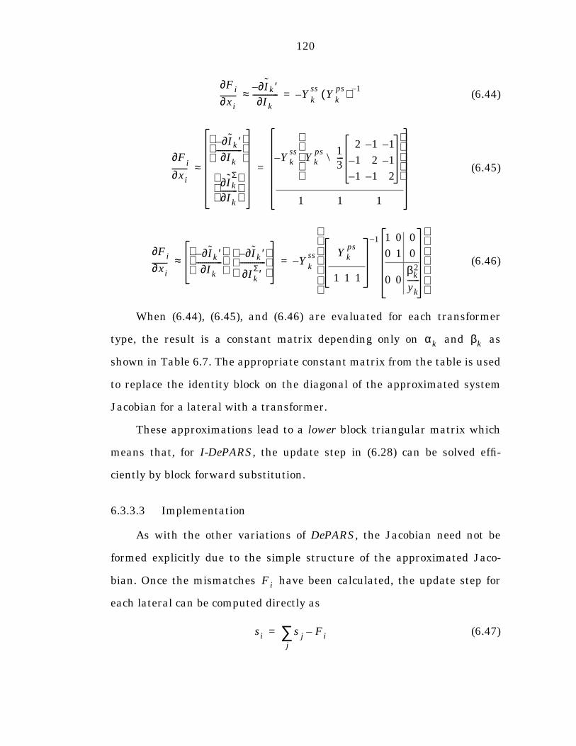
120

(6.44)

(6.45)

(6.46)

When (6.44), (6.45), and (6.46) are evaluated for each transformer

type, the result is a constant matrix depending only on and as

shown in Table 6.7. The appropriate constant matrix from the table is used

to replace the identity block on the diagonal of the approximated system

Jacobian for a lateral with a transformer.

These approximations lead to a lower block triangular matrix which

means that, for I-DePARS, the update step in (6.28) can be solved effi-

ciently by block forward substitution.

6.3.3.3 Implementation

As with the other variations of DePARS, the Jacobian need not be

formed explicitly due to the simple structure of the approximated Jaco-

bian. Once the mismatches have been calculated, the update step for

each lateral can be computed directly as

(6.47)

xi∂∂Fi Ik′∂–

Ik∂-------------≈ Y

kss

Ykps( ) 1–

–=

xi∂∂F

i

Ik′∂–

Ik∂-------------

IkΣ

∂Ik∂

--------

≈Yk

ssYk

ps 13---

2 1– 1–

1– 2 1–

1– 1– 2

\

–

1 1 1

=

xi∂∂Fi Ik′∂–

Ik∂-------------

Ik′∂–

IkΣ′∂

-------------

≈ Ykss Yk

ps

1 1 1

1– 1 0 0

0 1 0

0 0βk

2

yk------

–=

αk βk

Fi

si s jj

∑ Fi–=

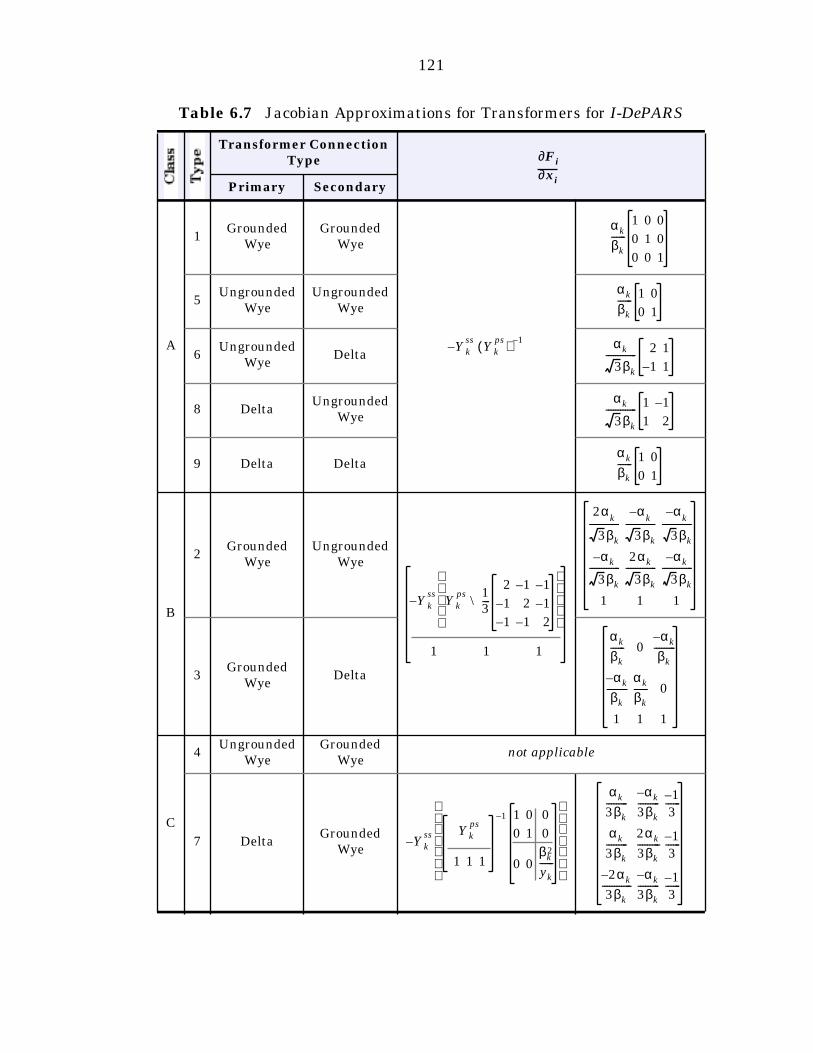
121

Table 6.7 Jacobian Approximations for Transformers for I-DePARS


Primary Secondary

A

1Grounded

WyeGrounded

Wye

5Ungrounded

WyeUngrounded

Wye

6Ungrounded

WyeDelta

8 DeltaUngrounded

Wye

9 Delta Delta

B

2Grounded

WyeUngrounded

Wye

3Grounded

WyeDelta

C

4Ungrounded

WyeGrounded

Wyenot applicable

7 DeltaGrounded

Wye

xi∂∂Fi

Ykss

Ykps( ) 1–

–

αk

βk

------1 0 0

0 1 0

0 0 1

αk

βk

------ 1 0

0 1

αk

3βk

------------- 2 1

1– 1

αk

3βk

------------- 1 1–

1 2

αk

βk

------ 1 0

0 1

Ykss

Ykps 1

3---

2 1– 1–

1– 2 1–

1– 1– 2

\

–

1 1 1

2αk

3βk

-------------α

k–

3βk

-------------α

k–

3βk

-------------

αk–

3βk

-------------2αk

3βk

-------------αk–

3βk

-------------

1 1 1

αk

βk

------ 0αk–

βk

---------

αk–

βk

---------αk

βk

------ 0

1 1 1

Ykss Yk

ps

1 1 1

1– 1 0 0

0 1 0

0 0βk

2

yk

------

–

αk

3βk

---------αk–

3βk

---------1–3------

αk

3βk

---------2αk

3βk

----------1–3------

2– αk

3βk

-------------αk–

3βk

---------1–3------

122

for laterals without transformers, and

(6.48)

for laterals with transformers. Here refers to the update step for

lateral j, where j is a sub-lateral of lateral i. The calculation of the update

steps must therefore proceed in RBF1 order.

One disadvantage to I-DePARS as compared to VI-DePARS is the

availability of a good starting value for the independent variable x. For

VI-DePARS the end voltages are set directly to balanced 1 per unit. How-

ever, some computation is required to find an initial value for the currents

injected into each lateral. This is typically done by current summation dur-

ing some type of backward sweep such as the one used in V-I-PARS.

6.3.4 S-DePARS

S-DePARS is the power flow based counterpart to I-DePARS and is a

generalization of the reduced power flow equations and fast decoupled

algorithm for radial systems first proposed in [12].

This approach is restricted to transformers of types 1, 5, and 9 which

have the same connection on both primary and secondary. For an ideal

transformer, there is no change in power from the primary to the second-

ary so an identity block is used for the corresponding diagonal block of the

system Jacobian. Unfortunately, for the other transformer connection

types there is no simple way to approximate the Jacobian, so they have not

been included in this formulation.

si xi∂

∂Fi

1–

sj

j∑ F

i–

=

s j

123

The approximate Jacobian for S-DePARS is identical to that of

I-DePARS. The update step in the Newton method can therefore be solved

by a block forward substitution.


In this section, it will be shown that the fast decoupled algorithms

described here fall into the class of inexact Newton methods discussed in

[14]. In the classical Newton’s method shown in Table 6.1, the update step

at iteration i is the solution to

. (6.49)

In the inexact Newton methods, the corresponding equation is

, (6.50)

where the size of the residual is restricted so that the relative residual

is bound by some forcing sequence. Specifically,

, (6.51)

where is a forcing sequence which is uniformly less than one. Here

denotes an arbitrary norm in . Notice that the special case where

gives the exact Newton’s method.

A sequence of iterates produced by the inexact Newton

method is locally and linearly convergent. This result is stated and proved

as Theorem 2.3 in [14]. Using the present notation, this theorem asserts

the following:

si( )

Ji( )

si( )

Fi( )

–=

Ji( )

si( )

Fi( )

– ri( )

+=

ri( )

ri( )

Fi( )--------------- η i( )≤

η i( ){ }

. IRn

η i( )0≡

xi( ){ }

124

Assume that . There exists such that, if

, then the sequence of inexact Newton iterates

converges to . Moreover, the convergence is linear in

the sense that

(6.52)

where .

For the fast decoupled methods presented here, the update step can

be expressed as the solution to

, (6.53)

where is the constant approximation, shown in Figure 6.4,12 to the Jaco-

bian . With the definition

, (6.54)

(6.53) can be rewritten in the form of the inexact Newton equation of

(6.50),

(6.55)

where the residual is .

To prove that DePARS is, in fact, an inexact Newton method, and

therefore locally and linearly convergent, it remains to be shown that there

is some sequence , uniformly less than one, which bounds the rela-

tive residual. This relative residual can now be expressed as

. (6.56)

12 Or, for I-DePARS and S-DePARS, the transpose of the matrix shown in Figure 6.4.

η i( ) ηmaxt 1< <≤ ε 0>

x0( )

x∗– ε≤x

i( ){ } x∗

xi 1+( )

x∗– J∗ t xi( )

x∗– J∗≤

yJ∗ J x∗( )y≡

Jsi( )

Fi( )

–=

J

Ji( )

∆Ji( )

Ji( )

J–≡

Ji( )

si( )

Fi( )

– ∆Ji( )

si( )

+=

ri( ) ∆J

i( )s

i( )=

η i( ){ }

ri( )

Fi( )---------------

∆Ji( )

si( )

Jsi( )-----------------------------=

125

For a network with only grounded wye to grounded wye transformers some

conclusions can be drawn about the size of this residual under the follow-

ing assumptions:

• All voltage magnitudes are close to 1 per unit.

• All transformer tap ratios are close to one.

• All per unit network parameters13 are small compared to voltage magnitudes (i.e. they are ).

Given these assumptions, is of the form shown in Figure 6.4,14

where all diagonal terms are equal to or nearly equal to one and the off-

diagonal non-zero terms are equal to minus one. The matrix in the

residual term is the difference between the true Jacobian, whose structure

is shown in Figure 6.3, and . This elements of this matrix are all small

compared to one. This implies that

, (6.57)

hence can be chosen such that

, (6.58)

thereby completing the proof that DePARS is a locally and linearly conver-

gent inexact Newton method.

13 This includes all line and transformer impedances, line charging admittances, shuntadmittances, constant Z load admittances, constant PQ load power injections, and cogen-erator power injections.

14 Figure 6.6 for I-DePARS and S-DePARS.

1«

J

∆Ji( )

J

∆Ji( )

si( )

Jsi( )----------------------------- 1«

ηi( )

∆Ji( )

si( )

Jsi( )

----------------------------- η i( )1< <

126

6.5 Comments

As with the backward/forward sweep methods of Chapter 5, the fast

decoupled methods are applicable to a wide range of radial distribution

networks. The one modeling limitation of the general DePARS formulation

is that it does not include type 4 ungrounded wye to grounded wye trans-

formers. One variation, S-DePARS, is further restricted to transformers of

types 1, 5, and 9, all of which have identical connection and grounding on

both primary and secondary sides.

As with BFS-PARS, the power flow based variations typically require

more computation per iteration than their current based counterparts.

Considering this difference and the fact that S-DePARS is limited to only

three types of transformer connections, VI-DePARS and I-DePARS appear

to be the most attractive of the four fast decoupled methods. VI-DePARS

has the added advantage of readily available initial values for the indepen-

dent variable x.

As with NR-PARS and BFS-PARS, the amount of computation

required per iteration is proportional to the number of buses. For a con-

stant number of iterations for convergence, the computational complexity

increases linearly with the size of the system, making DePARS effective for

very large radial distribution networks.

127

Chapter 7

Power Flow Algorithms for Weakly Meshed Systems (PAWMS)

The previous chapters have dealt with electric distribution systems

with a radial topological structure. The algorithms developed and pre-

sented in these chapters are specific to networks which do not contain any

loops. This chapter investigates an approach for extending these radial

algorithms to handle systems with a limited number of loops. The result-

ing class of algorithms will be referred to as Power flow Algorithms for

Weakly Meshed Systems, or PAWMS.

The approach taken by PAWMS requires that the meshed system be

converted to a radial structure by breaking each of the loops. The current

or power injections at each breakpoint are adjusted in order to balance the

voltages at either side using a compensation method [30]. Variations of this

method have been presented in [23], [19], and [20] for single-phase net-

works, and more recently in [11] for three-phase systems. The approach

presented here generalizes these to work with the various three-phase

radial power flow algorithms presented in this dissertation.

128

Apart from handling cases with loops, the compensation method also

makes it possible to solve systems with more than one voltage controlled

bus. These can be secondary sources with both voltage magnitude and

angle specified, or PV buses which specify voltage magnitude and real

power injection. First, the method of dealing with loops is described in

detail, followed by the modifications necessary for secondary sources and

PV buses.


Since PAWMS is based on a radial power flow solver, the weakly

meshed system must first be converted to a radial structure. This is done

by choosing a bus for each loop to serve as the breakpoint. Figure 7.1

shows a system with a loop containing bus k. This loop can be broken by

splitting bus k to create a new artificial bus . The solution of the original

meshed network is equivalent to the solution of the resulting radial system

under the constraints that and the current injection at bus is

the negative of the injection at bus k.

The actual creation of the artificial buses to break the loops is per-

formed once during the initialization process. The algorithm, after initial-

ization, consists of two steps which are repeated until convergence is

achieved, as shown in Table 7.1. First, the breakpoint voltages are updated

via a radial power flow method. Then, the current injections, at bus k

and at bus , are adjusted according to the breakpoint voltages in

order to eliminate any mismatch. The adjustment is based on the sensitiv-

ity of the breakpoint voltage mismatch to changes in the breakpoint cur-

rent injections. This sensitivity is approximated by the breakpoint

k′

Vk Vk′= k′

IBPj

I– BPj k′

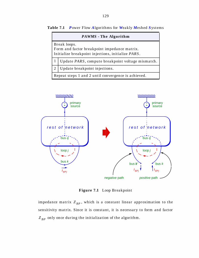
129

impedance matrix , which is a constant linear approximation to the

sensitivity matrix. Since it is constant, it is necessary to form and factor

only once during the initialization of the algorithm.

Table 7.1 Power Flow Algorithms for Weakly Meshed Systems

PAWMS - The Algorithm

Break loops.Form and factor breakpoint impedance matrix.Initialize breakpoint injections, initialize PARS.

1 Update PARS, compute breakpoint voltage mismatch.

2 Update breakpoint injections.

Repeat steps 1 and 2 until convergence is achieved.

Figure 7.1 Loop Breakpoint

r e s t o f n e t w o r k

bus kk ′ bus kbus k

loop j

IBPjIBPj IBPj

+– primary

loop j

+– primary

bus q


bus q

negative path positive path

sourcesource

ZBP

ZBP

130

7.1.1 Loop Breakpoint Creation

The primary issue in converting the meshed system to a radial net-

work is the choice of the loop breakpoint locations. As shown in Figure 7.1,

each loop can be divided into two pieces, both of which are supplied

through some common bus q. The positive path refers to the path between

bus q and the breakpoint bus k, and the negative path is the path between

bus q and the artificial bus . Some of the power supplied to the loop

through bus q will enter through the positive path and some through the

negative path depending on the branch impedances and the distribution of

the loads on the loop. For good convergence, the breakpoint location for a

loop should be chosen so as to minimize the breakpoint current .

Although it is not possible to choose a priori the breakpoint location

which will result in the smallest breakpoint current , it is easy to see

that a depth-first approach to finding and breaking loops would be a worst

case. In this case, the loop is detected after traversing the entire loop in

one direction and arriving again at bus q, which becomes the site of the

breakpoint. All of the load on the entire loop would be put on the negative

path and none on the positive path. Not only would this approach make it

difficult to estimate reasonable initial values for the breakpoint injections,

it would also cause unnecessary convergence problems for the radial power

flow solver due to the potentially tremendous load on one lateral.

Figure 7.2 shows that a much more reasonable and successful method

is to use a breadth-first approach to detecting and breaking loops. In this

case, both the positive and negative paths are traversed simultaneously

and the breakpoint is chosen as the bus farthest from the source. If bus k is

visited twice, coming from two different directions, a loop has been

k′

IBPj

IBPj

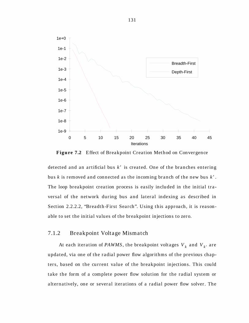
131

detected and an artificial bus is created. One of the branches entering

bus k is removed and connected as the incoming branch of the new bus .

The loop breakpoint creation process is easily included in the initial tra-

versal of the network during bus and lateral indexing as described in

Section 2.2.2.2, “Breadth-First Search”. Using this approach, it is reason-

able to set the initial values of the breakpoint injections to zero.

7.1.2 Breakpoint Voltage Mismatch

At each iteration of PAWMS, the breakpoint voltages and are

updated, via one of the radial power flow algorithms of the previous chap-

ters, based on the current value of the breakpoint injections. This could

take the form of a complete power flow solution for the radial system or

alternatively, one or several iterations of a radial power flow solver. The

Figure 7.2 Effect of Breakpoint Creation Method on Convergence

Iterations

1e-9

1e-8

1e-7

1e-6

1e-5

1e-4

1e-3

1e-2

1e-1

1e+0

0 5 10 15 20 25 30 35 40 45

Breadth-First

Depth-First

k′

k′

Vk Vk′

132

resulting breakpoint voltages are then used to compute the mismatch for

each loop j with breakpoint k.

(7.1)

Each complex three-phase voltage can be represented by

a 6 x 1 vector containing its real and imaginary parts.

(7.2)

The breakpoint voltage mismatch vector is formed by combining the

mismatches for each loop j as follows:

(7.3)

This is a x 1 real vector, where nlp is the number of loops in the

network.

7.1.3 Breakpoint Impedance Matrix

In order to update the breakpoint injections in a way which elimi-

nates the breakpoint voltage mismatches, it is necessary to know the corre-

sponding sensitivity information. A linear approximation to these

sensitivities is given by the breakpoint impedance matrix . For a

three-phase system, is a real, non-sparse, square matrix of dimension

.

∆V BPj Vk′ Vk–=

V E jF+=

V EF

=

∆V BP

∆V BPj

∆V BP

∆EBP1

∆FBP1

∆EBP2

∆FBP2

∆EBPnlp

∆FBPnlp

=

6 nlp⋅( )

ZBP

ZBP

6 nlp⋅( )

133

Let each complex three-phase current also be represented

by a 6 x 1 vector of its real and imaginary parts, however, with the imagi-

nary part negated.

(7.4)

The reason for this separation into real and imaginary parts will be seen

clearly in Section 7.1.6, “PV Buses”. The breakpoint currents for each

loop j are then combined to form the x 1 real breakpoint injection

vector

(7.5)

The breakpoint impedance matrix is an approximation of the

sensitivity of to changes in . This relationship can be written

(7.6)

The matrix consists of 6 x 6 block elements corresponding to

loops i and j. These blocks can be constructed directly according to the fol-

lowing observations:

I C jD+=

I C

D–=

IBPj

6 nlp⋅( )

IBP

CBP1

DBP1–

CBP2

DBP2

–

CBPnlp

DBPnlp–

=

ZBP

∆VBP

IBP

∆VBP

ZBP

∆IBP

=

ZBP ZBPij

134

• For diagonal blocks where , is the sum of the branch impedances in loop i.

• For off-diagonal blocks where , the magnitude of is the sum of the impedances of branches common to loops i and j. The sign is negative if the loops have opposite direction and positive if they have the same direction.1

To be consistent with the representations of voltage and current in (7.2)

and (7.4), the branch impedances are represented as

(7.7)

Since is constant, it is only formed once at the beginning of the

algorithm. It can also be factored once via LU decomposition as

(7.8)

and its triangular factors and stored for later use in solving for

from (7.6).

7.1.4 Breakpoint Injections

The second part of each iteration of PAWMS is to update the break-

point current injections. This involves solving for from the set of lin-

ear equations in (7.6) via backward and forward substitution using the

triangular factors from (7.8).

(7.9)

The appropriate element is then added as a correction to the

current value of the injection for loop j.

(7.10)

1 The direction of a loop is arbitrarily defined to be toward the source on the positivepath and away from the source on the negative path. This is also the convention used forthe direction of the breakpoint current as shown in Figure 7.1.

i j= ZBPij

i j≠ ZBPij

Z R jX+=

Z R X

X R–=

ZBP

ZBP

LBP

UBP

⋅→

LBP UBP

∆IBP

∆IBP

∆IBP UBP LBP ∆V BP\( )\=

∆IBPj

IBPj IBPj ∆IBPj+←

135

These new current injections are used with positive and negative signs,

respectively, at the corresponding breakpoint buses and k during the

next radial power flow update.

7.1.5 Multiple Sources

Throughout the preceding chapters of this dissertation, it has always

been assumed that the network under consideration has a single voltage

specified bus denoted as the source. The compensation method used to deal

with loops in a system can also be applied to the problem of multiple

sources. In a network with multiple sources, one of them is arbitrarily cho-

sen as the primary source and is used as the source for the purposes of the

radial load flow algorithms.

Each of the other secondary sources is treated as a normal load bus

with an extra current injection. For a secondary source at bus k, the volt-

age constraint creates a loop j through ground, which can be broken as

shown in Figure 7.3.

In this case, the artificial bus need not be created explicitly. The

voltage mismatch for a secondary source at bus k is simply

. (7.11)

The corresponding breakpoint current injection is the current injected

into the system at bus k by the secondary source. Although the negative

path of a loop formed by a secondary source has no impedance, the forma-

tion of the breakpoint impedance matrix does not change from the

method described above for simple loops.

k′

k′

∆V BPj

∆V BPj Vkspecified

Vk–=

IBPj

ZBP

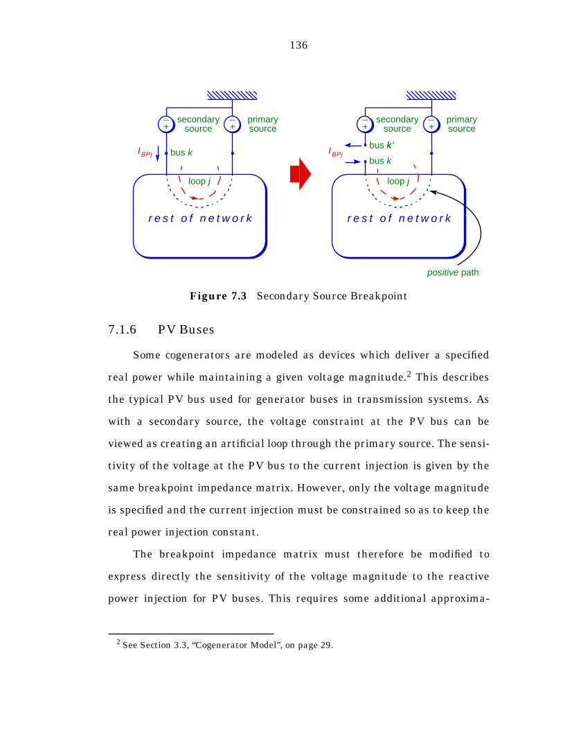
136

7.1.6 PV Buses

Some cogenerators are modeled as devices which deliver a specified

real power while maintaining a given voltage magnitude.2 This describes

the typical PV bus used for generator buses in transmission systems. As

with a secondary source, the voltage constraint at the PV bus can be

viewed as creating an artificial loop through the primary source. The sensi-

tivity of the voltage at the PV bus to the current injection is given by the

same breakpoint impedance matrix. However, only the voltage magnitude

is specified and the current injection must be constrained so as to keep the

real power injection constant.

The breakpoint impedance matrix must therefore be modified to

express directly the sensitivity of the voltage magnitude to the reactive

power injection for PV buses. This requires some additional approxima-

2 See Section 3.3, “Cogenerator Model”, on page 29.

Figure 7.3 Secondary Source Breakpoint

bus kk ′bus kIBPj

+– primary


loop j

positive path

source+– secondary

source

bus kIBPj

+– primary


loop j

source+– secondary

source

137

tions and a change of basis for voltage and current vectors V and I, and

impedance matrices Z, as given in (7.2), (7.4), and (7.7).

Define a rotation matrix U to rotate phases b and c by 120° and -120°,

respectively,

, (7.12)

where , and note that

. (7.13)

For 3 x 1 complex vectors V and I, and 3 x 3 complex matrix Z, let

(7.14)

(7.15)

(7.16)

This set of definitions corresponds to a change of basis or rotation of the

phase b and phase c voltages and currents.

Assuming a three-phase network with a balanced 1 per unit primary

source and no phase shifts, the magnitude of each element of is equal to

the magnitude of the corresponding element of V and is therefore close to

1 per unit. The angles of the elements of , however, are all nearly

zero, leading to the following approximations to the real and imaginary

parts of .

U1 0 0

0 α 0

0 0 α2

=

α ej2π3

------ 12---– j

32

-------+= =

U 1– U∗1 0 0

0 α2 0

0 0 α

= =

V′ UV≡

I′ UI≡

Z′ UZU 1–≡

V′

θ′ V′

V′ E′ jF ′+=

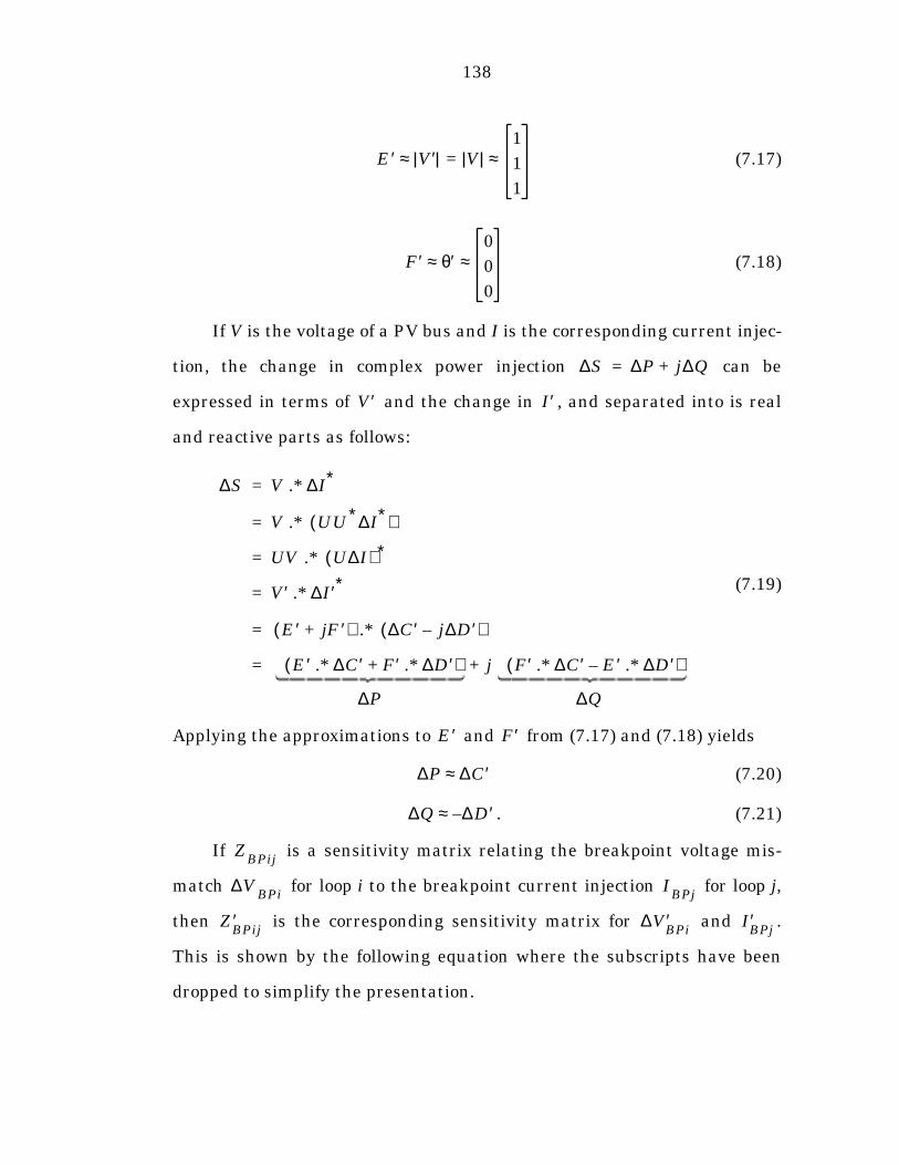
138

(7.17)

(7.18)

If V is the voltage of a PV bus and I is the corresponding current injec-

tion, the change in complex power injection can be

expressed in terms of and the change in , and separated into is real

and reactive parts as follows:

(7.19)

Applying the approximations to and from (7.17) and (7.18) yields

(7.20)

. (7.21)

If is a sensitivity matrix relating the breakpoint voltage mis-

match for loop i to the breakpoint current injection for loop j,

then is the corresponding sensitivity matrix for and .

This is shown by the following equation where the subscripts have been

dropped to simplify the presentation.

E′ V′ V1

1

1

≈=≈

F′ θ′0

0

0

≈ ≈

∆S ∆P j∆Q+=

V′ I′

∆S V ∆I∗.*

V UU∗∆I∗( ).*

UV U∆I( ) ∗.*

V′ ∆I′∗.*

E′ jF ′+( ) ∆C′ j∆D′–( ).*

E′ ∆C′.* F′ ∆D′.*+( ) j F′ ∆C′.* E′ ∆D′.*–( )+

=

=

=

=

=

=

∆Q∆P

E′ F′

∆P ∆C′≈

∆Q ∆– D′≈

ZBPij

∆VBPi

IBPj

Z′BPij

∆V′BPi

I′BPj

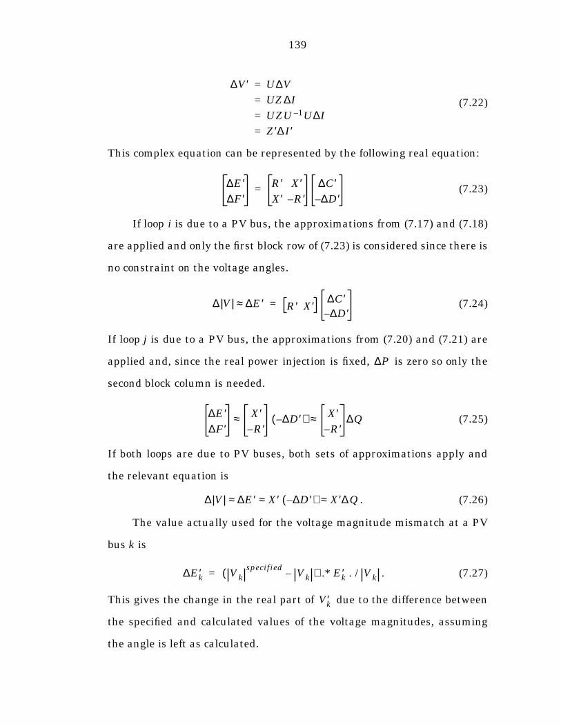
139

(7.22)

This complex equation can be represented by the following real equation:

(7.23)

If loop i is due to a PV bus, the approximations from (7.17) and (7.18)

are applied and only the first block row of (7.23) is considered since there is

no constraint on the voltage angles.

(7.24)

If loop j is due to a PV bus, the approximations from (7.20) and (7.21) are

applied and, since the real power injection is fixed, is zero so only the

second block column is needed.

(7.25)

If both loops are due to PV buses, both sets of approximations apply and

the relevant equation is

. (7.26)

The value actually used for the voltage magnitude mismatch at a PV

bus k is

. (7.27)

This gives the change in the real part of due to the difference between

the specified and calculated values of the voltage magnitudes, assuming

the angle is left as calculated.

∆V′ U∆V

UZ∆I

UZU 1– U∆I

Z′∆I′

=

=

=

=

∆E′∆F′

R′ X′X′ R′–

∆C′∆D′–

=

∆ V ∆E′≈ R′ X′∆C′∆D′–

=

∆P

∆E′∆F′

X′R′–

∆D′–( ) X′R′–

∆Q≈ ≈

∆ V ∆E′ X′ ∆D′–( ) X′∆Q≈ ≈ ≈

∆E′k Vkspecified

Vk–( ) E′k Vk. /.*=

V′k

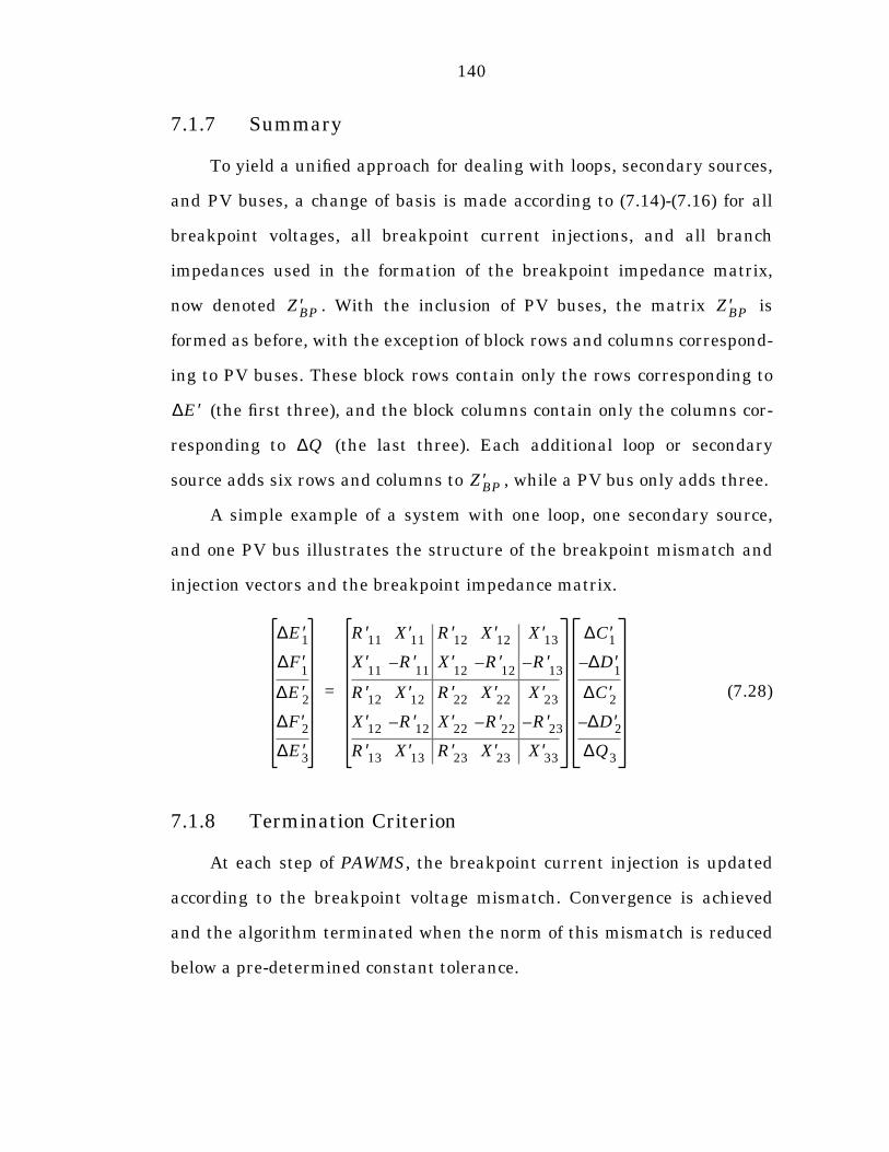
140

7.1.7 Summary

To yield a unified approach for dealing with loops, secondary sources,

and PV buses, a change of basis is made according to (7.14)-(7.16) for all

breakpoint voltages, all breakpoint current injections, and all branch

impedances used in the formation of the breakpoint impedance matrix,

now denoted . With the inclusion of PV buses, the matrix is

formed as before, with the exception of block rows and columns correspond-

ing to PV buses. These block rows contain only the rows corresponding to

(the first three), and the block columns contain only the columns cor-

responding to (the last three). Each additional loop or secondary

source adds six rows and columns to , while a PV bus only adds three.

A simple example of a system with one loop, one secondary source,

and one PV bus illustrates the structure of the breakpoint mismatch and

injection vectors and the breakpoint impedance matrix.

(7.28)


At each step of PAWMS, the breakpoint current injection is updated

according to the breakpoint voltage mismatch. Convergence is achieved

and the algorithm terminated when the norm of this mismatch is reduced

below a pre-determined constant tolerance.

Z′BP Z′BP

∆E′

∆Q

Z′BP

∆E′1∆F′

1

∆E′2∆F′2∆E′3

R′11 X′11 R′12 X′12 X′13

X′11

R′11

– X′12

R′12

– R′13

–

R′12 X′12 R′22 X′22 X′23

X′12 R′12– X′22 R′22– R′23–

R′13 X′13 R′23 X′23 X′33

∆C′1∆D′

1–

∆C′2∆D′2–

∆Q3

=

141

7.2 Implementation

Since the compensation method used to eliminate breakpoint voltage

mismatches is independent of the radial power flow algorithm used to com-

pute these mismatches, this independence was preserved in the implemen-

tation. The program was structured in a way which allows any of the

variations of NR-PARS, BFS-PARS, or DePARS to be used as the radial

solver.

7.2.1 Modeling Limitations and Simplifying Assumptions

The algorithm used to form the breakpoint impedance matrix is based

closely on the one from [20]. Since this method builds the matrix directly

from sums of branch impedances, it is not suited to loops which contain

some grounded and some ungrounded sections. For this reason, the imple-

mentation was restricted to networks with only type 1 grounded wye to

grounded wye transformers.

To simplify the code, the following additional assumptions were made.

All loops, including those formed by secondary sources and PV buses, are

three-phase only. This eliminates the need to deal with different dimen-

sions for breakpoint voltages and injections. It is also assumed that no two

loops result in a breakpoint at the same bus, preventing the need for a

variable number of breakpoint injection vectors for any given bus.

7.2.2 Termination of Radial Power Flow

Each iteration of PAWMS requires the computation of the breakpoint

voltage mismatch via one of the radial power flow algorithms presented in

previous chapters. However, depending on the tolerance used for the radial

142

power flow convergence criterion, a completely converged result may not be

necessary, especially in the first several iterations of PAWMS. In fact, in

some cases, a single iteration of the radial power flow may be sufficient to

achieve satisfactory convergence for PAWMS.

As implemented, the program allows for three possible modes of oper-

ation. In addition to converged sets and single iterations of the radial

power flow, an adaptive method is also included. This adaptive strategy is

based on a heuristic which attempts to set the tolerance for the radial

power flow for a given iteration such that the breakpoint voltage mis-

matches computed are only as accurate as necessary.

Using the maximum change in bus voltage as the mismatch for the

radial solver, a tolerance of typically results in bus voltages accurate

to about . This is generally sufficient for the computation of

breakpoint mismatches on the order of . An estimate of the breakpoint

voltage mismatch at the next iteration can therefore be used as a reason-

able tolerance for the current radial power flow. This estimate is readily

computed from the current breakpoint voltage mismatch and the current

rate of convergence, as calculated from the current and previous mis-

matches. This is the approach used by the adaptive method implemented

in the program.

7.3 Variations

Several modifications to the basic PAWMS presented here have been

considered. They are based primarily on the various approaches presented

in [23], [19], and [20] for single-phase power flow in weakly meshed sys-

tems.

10 n–

10 n 1+( )–

10 n–

143

7.3.1 Power Injection for Loop Breakpoints

It is possible to use power injection instead of current injection at the

loop breakpoints. This, obviously, does not affect the treatment of PV buses

and, in fact, has no effect for secondary sources as well, since their voltages

are fixed. For a simple loop j with breakpoint k, however, the voltage mis-

match is used to compute a correction to the injected current which is con-

verted to a correction to the injected power according to the following

equation:

(7.29)

In practice, this produces much better results than the more obvious

update

, (7.30)

as shown in Figure 7.4.

For a system with a mixed load model, there is little difference in per-

formance between the method based on breakpoint power injection and

that based on current injection. In general, using current injection yields

equivalent or slightly better convergence results. The largest difference is

seen in a system with purely constant current loads, and no shunt compo-

nents or cogenerators. In this case, the current-based PAWMS converges in

a single iteration since the network is linear and the breakpoint impedance

matrix is the exact sensitivity matrix.

∆SBPj

Vk Vk′+

2----------------------

∆IBPj∗.*

V′k V′k′+

2----------------------

∆I′BPj

∗.*

=

=

∆S ∆C′ j∆D′–=

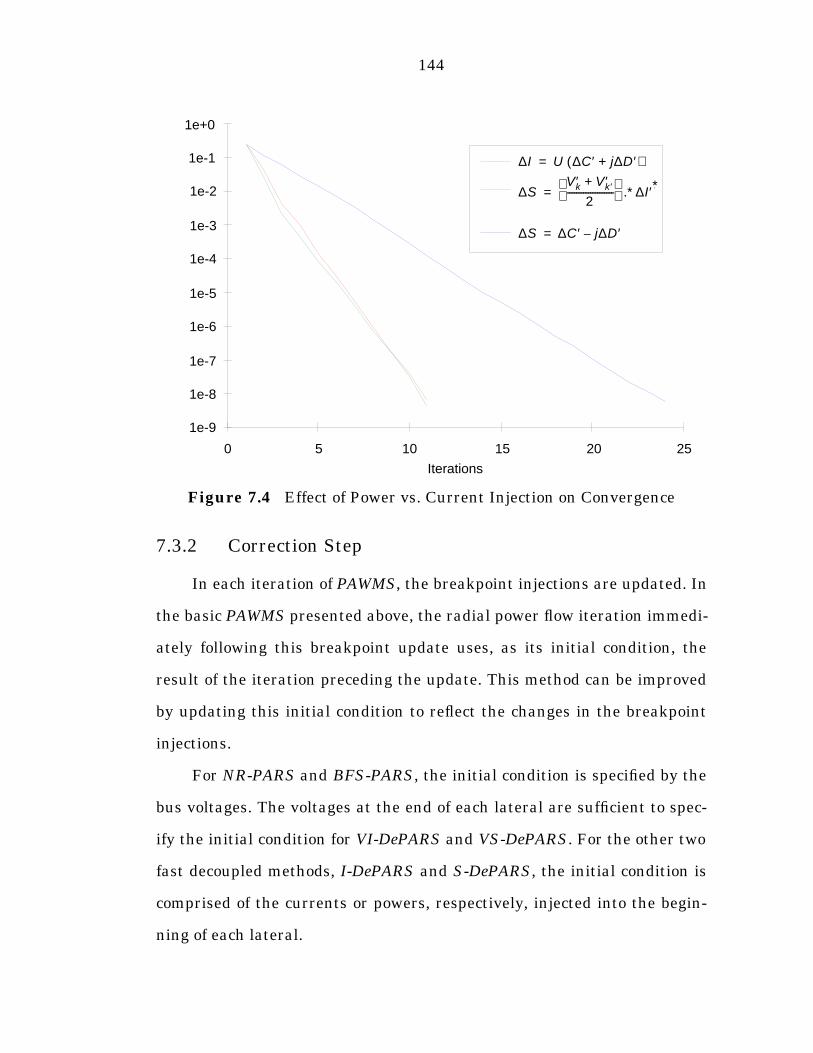
144

7.3.2 Correction Step

In each iteration of PAWMS, the breakpoint injections are updated. In

the basic PAWMS presented above, the radial power flow iteration immedi-

ately following this breakpoint update uses, as its initial condition, the

result of the iteration preceding the update. This method can be improved

by updating this initial condition to reflect the changes in the breakpoint

injections.

For NR-PARS and BFS-PARS, the initial condition is specified by the

bus voltages. The voltages at the end of each lateral are sufficient to spec-

ify the initial condition for VI-DePARS and VS-DePARS. For the other two

fast decoupled methods, I-DePARS and S-DePARS, the initial condition is

comprised of the currents or powers, respectively, injected into the begin-

ning of each lateral.

Figure 7.4 Effect of Power vs. Current Injection on Convergence

Iterations

1e-9

1e-8

1e-7

1e-6

1e-5

1e-4

1e-3

1e-2

1e-1

1e+0

0 5 10 15 20 25

∆I = U(∆C'+j∆D')

∆S = (V1+V2)/2 *conj(∆I)

∆S = ∆C'-j∆D'∆S ∆C′ j∆D′–=

∆SV′k V′k ′+

2--------------------

∆I′∗.*=

∆I U ∆C′ j∆D′+( )=

145

First consider the correction for NR-PARS and BFS-PARS. This volt-

age correction step adjusts the bus voltages to reflect the change in the

breakpoint injections according to the method presented in [20]. A back-

ward/forward sweep of the radial network is performed with:

• all loads, shunts, and cogenerators disconnected

• breakpoint injections set to their incremental values (the change in injection just computed)

• source voltage set to zero

The bus voltages computed from this process are incremental values

reflecting the change in bus voltages due to the change in breakpoint injec-

tion. These incremental voltages are added to the bus voltages from the

previous radial power flow iteration, resulting in a better starting point for

the new radial power flow.

For VI-DePARS and VS-DePARS, each iteration consists of a mis-

match evaluation followed by an update to the end voltages. The voltage

correction step described above can be used to calculate the incremental

voltages. In this case, it is only necessary to add the incremental values to

the end voltages since they are used to update all other bus voltages in the

succeeding mismatch evaluation.

When using I-DePARS and S-DePARS, the breakpoint injections are

updated immediately following a function evaluation. Each iteration of the

radial power flow then begins with the update to the independent vari-

ables, based on the mismatch from the previous iteration, and ends with

the evaluation of a new mismatch. It is convenient to switch this order

from that used by the other two DePARS methods above to allow for a mis-

match correction to adjust for the change in breakpoint injections.

146

The effect of a change in the injection at a particular breakpoint then

is simply to increase the corresponding lateral’s mismatch by the amount

of the change. The only other detail is that, for I-DePARS, incremental

power injections are converted to their approximate current equivalents3

before adding them to the appropriate mismatch. Likewise, for S-DePARS,

incremental current injections are converted to their approximate power

equivalents.3

The effect of adding a correction step to PAWMS is to improve the

overall convergence characteristics of the algorithm. Using the correction

step typically reduces the total number of radial power flow iterations

required to solve the weakly meshed power flow.

7.4 Comments

For a distribution system with a small number of loops, secondary

sources, and PV buses, the size of the breakpoint impedance matrix is rela-

tively small. The computation involved in forming and factoring the matrix

is still relatively small compared to the work required for the solution of

the radial system. However, as the number of loops grows, the computa-

tional burden associated with the breakpoint impedance matrix grows.

Since is, in general, not necessarily sparse, at some point, as the num-

ber of loops increases, the work associated with becomes so large that

it is more efficient to use a general nodal approach, such as the traditional

Newton-Raphson or Implicit Zbus Gauss methods. For this reason, PAWMS

is well suited to weakly meshed systems, but less well suited to the highly

connected structure of a typical transmission network.

3 Based on balanced 1 per unit voltages.

ZBP

ZBP

147

Another issue raised by extending a radial power flow technique to

handle weakly meshed systems is that of the existence and uniqueness of

solutions. According to [13], a typical radial distribution network always

has a unique feasible power flow solution. On the other hand, it is a well-

known fact that a meshed transmission network may have many feasible

steady-state equilibrium points or none at all. The solution found by

PAWMS for a weakly meshed distribution network may therefore not be a

unique feasible solution. Presumably, choosing a different initial value for

the breakpoint injections could result in a different solution to the power

flow problem. Furthermore, divergence of the algorithm in certain cases

could be due to the lack of a feasible solution.

148

Chapter 8

Simulation Results

All of the algorithms under consideration were implemented in a pro-

gram written for MATLAB®.1 The program reads the network data once

from a text file and then stores it in binary format for later use. After read-

ing the network data, either from the original text file or from the binary

file, the network is traversed as described in Section 2.2.2.2, “Breadth-

First Search”. During this traversal the nodes and laterals are indexed,

data is verified for consistency, and sections are marked as grounded or

ungrounded. Since it is common to all of the methods, this preprocessing

step is omitted from the comparison of computational effort associated

with each algorithm.

MATLAB® is a high-level interpreted language designed with matrix

manipulation in mind. The version used for this implementation,

version 4, includes sparse matrix storage and manipulation as built-in

functions. These capabilities made it an attractive choice for quick imple-

mentation and testing of ideas during the stage of algorithm development.

1 MATLAB® is a trademark of The MathWorks, Inc.

149

For the analysis of the algorithms, the interpreted nature of MATLAB®

makes it ideal for observing the behavior of individual parameters. On the

other hand, an interpreted language is usually quite a bit slower in execu-

tion than the compiled languages typically used for power flow, such as

Fortran or C. For this reason, MATLAB® is probably not the language of

choice for a program intended for use in industry. On a sufficiently fast

workstation, however, computation time for this implementation was not a

problem even with networks of more than 1000 buses.

The goal of this analysis of the results of the MATLAB® simulation is to

draw some meaningful conclusions about the behavior of the algorithms in

a compiled language, such as Fortran or C. This entails comparisons of the

effectiveness of each of the algorithms presented in Chapter 4 through

Chapter 7 relative to one another and relative to other relevant power flow

algorithms.

For this purpose, computation time in MATLAB® is nearly meaning-

less. In MATLAB®, solving a set of linear equations is a built-in function and

therefore executes at approximately the same speed as Fortran or C. Sim-

ple loops, however, are many times slower since each line is interpreted

each time through the loop. Consequently, the run time of an algorithm in

MATLAB® may be completely unrelated to the run time of the same algo-

rithm in Fortran or C. The number of floating point operations (flops)

required, though not a perfect measure, is chosen as a much better indica-

tor of relative run time in a compiled language.

150

8.1 Summary of Algorithms Tested

The simulations performed involve 16 different algorithms which can

be classified into the following four categories:

• traditional algorithms for the standard formulation (Newton-Raphson, Implicit Zbus Gauss)

• network reduction methods (NR-PARS)

• backward/forward sweep methods (BFS-PARS)

• fast decoupled methods (DePARS)

These algorithms are summarized in Table 8.1. The first class,

included for the sake of comparison, consists of standard power flow meth-

ods applied to the traditional power flow formulation for general meshed

systems. The remaining three classes are for radial networks only and are

collectively referred to as PARS (Power flow Algorithms for Radial Sys-

tems). Each variation of PARS can be extended, as described in Chapter 7,

to solve the power flow for weakly meshed networks. When a particular

version of PARS is used in conjunction with these extensions, the “PARS”

in the name of the algorithm is simply changed to “PAWMS” (Power flow

Algorithms for Weakly Meshed Systems).

Since the two traditional distribution power flow algorithms tested,

Newton-Raphson and Implicit Zbus Gauss, have not been discussed in pre-

vious chapters, each of them will be described briefly.

8.1.1 Newton-Raphson Method

The traditional formulation of the distribution power flow problem is

a set of power balance equations at each load bus as a function of the bus

voltages. Let be the vector of net power injected into the system at

Ybus

Sbus

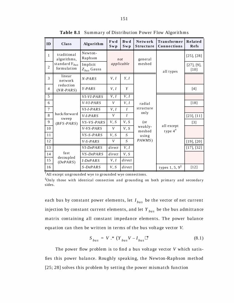
151

each bus by constant power elements, let be the vector of net current

injection by constant current elements, and let be the bus admittance

matrix containing all constant impedance elements. The power balance

equation can then be written in terms of the bus voltage vector V.

(8.1)

The power flow problem is to find a bus voltage vector V which satis-

fies this power balance. Roughly speaking, the Newton-Raphson method

[25; 28] solves this problem by setting the power mismatch function

†All except ungrounded wye to grounded wye connections.‡Only those with identical connection and grounding on both primary and secondarysides.

Table 8.1 Summary of Distribution Power Flow Algorithms

ID Class AlgorithmFwdSwp

BwdSwp

NetworkStructure

TransformerConnections

Related Refs

1 traditional algorithms,

standard Ybus formulation

Newton-Raphson not

applicablegeneral meshed

all types

[25], [28]

2Implicit Zbus Gauss

[27], [9], [10]

3linear

networkreduction

(NR-PARS)

N-PARS V, I Y, I

radial structure

only

(or weakly-meshed using

PAWMS)

4 Y-PARS V, I Y [4]

5

back/forwardsweep

(BFS-PARS)

VI-VI-PARS V, I V, I

all except

type 4†

6 V-VI-PARS V V, I [18]

7 VI-I-PARS V, I I

8 V-I-PARS V I [23], [11]

9 VS-VS-PARS V, S V, S [3]

10 V-VS-PARS V V, S

11 VS-S-PARS V, S S

12 V-S-PARS V S [19], [20]

13

fast decoupled(DePARS)

VI-DePARS direct V, I [17], [32]

14 VS-DePARS direct V, S

15 I-DePARS V, I direct

16 S-DePARS V, S direct types 1, 5, 9‡ [12]

Ibus

Ybus

Sbus

V Ybus

V Ibus

–( ) ∗.*=

152

(8.2)

to zero and solving for the roots via Newton’s method.2 To be more accu-

rate, the set of equations given to Newton’s method consists of only the

rows of (8.2) associated with the load buses. Similarly, the unknowns are

the bus voltages at the load buses, since the source voltage is assumed to

be given.

8.1.2 Implicit Zbus Gauss Method

The Implicit Zbus Gauss method [27; 9; 10] also uses a standard

formulation. At all times, the state of a power system must satisfy

Kirchhoff’s current law at every bus. This constraint can be expressed as

(8.3)

where I is the vector of current injected by all constant current and con-

stant power elements. The voltage and current vectors are separated into

two parts, the first corresponding to the source and the second correspond-

ing to the remaining buses.

(8.4)

In this case, the power flow problem is to solve for , given the

source voltage . If the circuit contains no constant power elements, is

a known constant injection and can be found directly from the lower

part of (8.4).

(8.5)

2 See Table 6.1, “Newton’s Method”, on page 86.

F V( ) V YbusV Ibus–( ) ∗.* Sbus– 0= =

Ybus

I YbusV=

I1

I2

Y11 Y12

Y21 Y22

V1

V2

=

V2

V1 I2

V2

V2 Y221– I2 Y21V1–( )=

153

This is a simple linear circuit solution via a nodal method. If the network

contains constant power devices, they can be linearized by replacing them

with equivalent current injections based on an estimate of the bus volt-

ages. In this case, the current injection becomes a function of the bus

voltage vector .

(8.6)

The Gauss method can be applied to solve this equation by repeatedly

updating , evaluating the right hand side using the most recent value of

. When the change in between iterations is smaller than some toler-

ance the algorithm is terminated. This is called a “Zbus” method since it is

equivalent to repeatedly multiplying by the impedance matrix . In

practice, since this matrix is not sparse, it is not necessary or desirable to

explicitly form it, hence the “implicit” in the name of the algorithm.

Instead, is factored once via an LU decomposition and its factors are

stored. The evaluation of the right hand side of (8.6) then consists of com-

puting and doing a backward and forward substitution using the

factored matrix.

The primary differences between the implementation used for the

tests presented in this chapter and the version described in [9] and [10] are

the following. In this implementation, all constant impedance elements,

including transformers, shunt capacitors, and constant impedance loads,

are included in . It is possible to include transformers without encoun-

tering the ill-conditioning problems mentioned in [10] since this implemen-

tation is based on only solving for line-to-line voltages in ungrounded

sections of the network.

I2

V2

V2

Y22

1– I2

V2

( ) Y21

V1

–( )=

V2

V2 V2

Y221–

Y22

I2 V2( )

Ybus

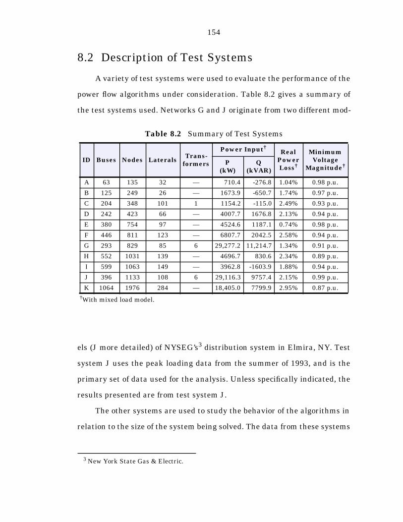
154

8.2 Description of Test Systems

A variety of test systems were used to evaluate the performance of the

power flow algorithms under consideration. Table 8.2 gives a summary of

the test systems used. Networks G and J originate from two different mod-

els (J more detailed) of NYSEG’s3 distribution system in Elmira, NY. Test

system J uses the peak loading data from the summer of 1993, and is the

primary set of data used for the analysis. Unless specifically indicated, the

results presented are from test system J.

The other systems are used to study the behavior of the algorithms in

relation to the size of the system being solved. The data from these systems

†With mixed load model.

3 New York State Gas & Electric.

Table 8.2 Summary of Test Systems

ID Buses Nodes LateralsTrans-

formers

Power Input†Real

PowerLoss†

MinimumVoltage

Magnitude†P(kW)

Q(kVAR)

A 63 135 32 — 710.4 -276.8 1.04% 0.98 p.u.

B 125 249 26 — 1673.9 -650.7 1.74% 0.97 p.u.

C 204 348 101 1 1154.2 -115.0 2.49% 0.93 p.u.

D 242 423 66 — 4007.7 1676.8 2.13% 0.94 p.u.

E 380 754 97 — 4524.6 1187.1 0.74% 0.98 p.u.

F 446 811 123 — 6807.7 2042.5 2.58% 0.94 p.u.

G 293 829 85 6 29,277.2 11,214.7 1.34% 0.91 p.u.

H 552 1031 139 — 4696.7 830.6 2.34% 0.89 p.u.

I 599 1063 149 — 3962.8 -1603.9 1.88% 0.94 p.u.

J 396 1133 108 6 29,116.3 9757.4 2.15% 0.99 p.u.

K 1064 1976 284 — 18,405.0 7799.9 2.95% 0.87 p.u.

155

are derived from models provided by Rochester Gas & Electric in NY.

Except for the tests which explicitly examine the effect of the load model,

all of the tests are run with a random mixture of approximately equal

numbers of constant PQ, constant current, and constant impedance loads.

8.3 Power Flow Algorithms for Radial Systems (PARS)

This section examines the performance of each of the power flow algo-

rithms described in this dissertation as applied to strictly radial systems.

As certain variations of the algorithms are found to be inferior, they are

then excluded from further tests and analysis.

First, consider a comparison of the number of iterations required by

the various algorithms to solve test systems B and J for a mixed load

model, as shown in Figure 8.1. With a few exceptions, the algorithms

require between about five and ten iterations to converge. The Newton-

Raphson method on average requires fewer iterations due to its quadratic

convergence property. The remaining algorithms exhibit what appears to

be linear convergence. Figure 8.2 illustrates this difference for a represen-

tative subset of the methods. It should be noted that the number of itera-

tions required by Implicit Zbus Gauss and N-PARS are always identical

since both methods solve the same linear approximation to the circuit at

each iteration.

Despite its superior performance with regard to number of iterations,

Figure 8.3 shows that the total number of flops required by the Newton-

Raphson method is approximately an order of magnitude greater, on aver-

age, than required by the remaining methods. In the network reduction

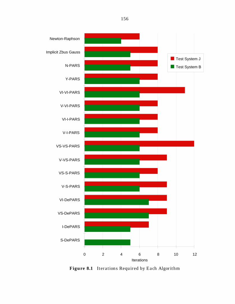
156

Figure 8.1 Iterations Required by Each Algorithm

Iterations

0 2 4 6 8 10 12

Newton-Raphson

Implicit Zbus Gauss

N-PARS

Y-PARS

VI-VI-PARS

V-VI-PARS

VI-I-PARS

V-I-PARS

VS-VS-PARS

V-VS-PARS

VS-S-PARS

V-S-PARS

VI-DePARS

VS-DePARS

I-DePARS

S-DePARS

Test System J

Test System B

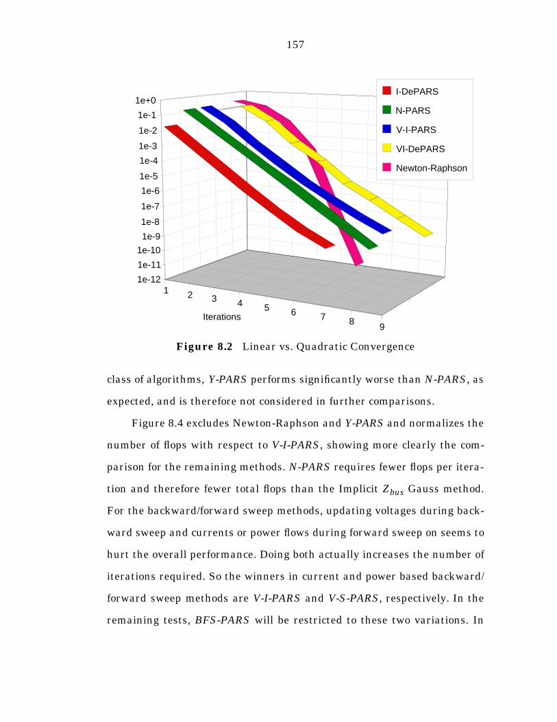
157

class of algorithms, Y-PARS performs significantly worse than N-PARS, as

expected, and is therefore not considered in further comparisons.

Figure 8.4 excludes Newton-Raphson and Y-PARS and normalizes the

number of flops with respect to V-I-PARS, showing more clearly the com-

parison for the remaining methods. N-PARS requires fewer flops per itera-

tion and therefore fewer total flops than the Implicit Zbus Gauss method.

For the backward/forward sweep methods, updating voltages during back-

ward sweep and currents or power flows during forward sweep on seems to

hurt the overall performance. Doing both actually increases the number of

iterations required. So the winners in current and power based backward/

forward sweep methods are V-I-PARS and V-S-PARS, respectively. In the

remaining tests, BFS-PARS will be restricted to these two variations. In

Figure 8.2 Linear vs. Quadratic Convergence

1 2 3 4 5 6 7 89

Iterations

1e-12

1e-11

1e-10

1e-9

1e-8

1e-7

1e-6

1e-5

1e-4

1e-3

1e-2

1e-1

1e+0I-DePARS

N-PARS

V-I-PARS

VI-DePARS

Newton-Raphson

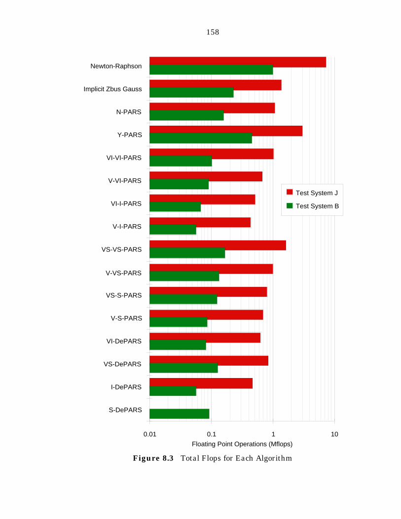
158

Figure 8.3 Total Flops for Each Algorithm

Floating Point Operations (Mflops)

0.01 0.1 1 10

Newton-Raphson

Implicit Zbus Gauss

N-PARS

Y-PARS

VI-VI-PARS

V-VI-PARS

VI-I-PARS

V-I-PARS

VS-VS-PARS

V-VS-PARS

VS-S-PARS

V-S-PARS

VI-DePARS

VS-DePARS

I-DePARS

S-DePARS

Test System J

Test System B

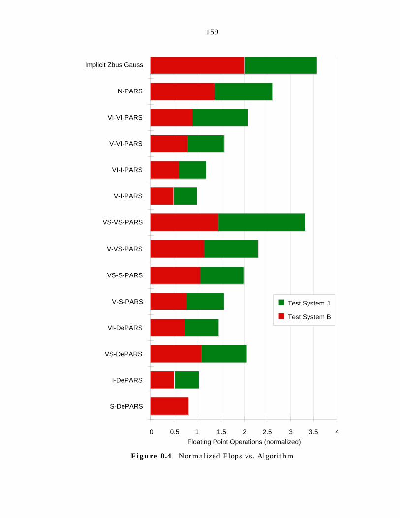
159

Figure 8.4 Normalized Flops vs. Algorithm

Floating Point Operations (normalized)

0 0.5 1 1.5 2 2.5 3 3.5 4

Implicit Zbus Gauss

N-PARS

VI-VI-PARS

V-VI-PARS

VI-I-PARS

V-I-PARS

VS-VS-PARS

V-VS-PARS

VS-S-PARS

V-S-PARS

VI-DePARS

VS-DePARS

I-DePARS

S-DePARS

Test System J

Test System B

160

the fast decoupled class, I-DePARS appears most attractive. In fact, due to

the limitations on the types of transformers handled by S-DePARS, it is

unable to solve test system J and is therefore also removed from further

consideration.

8.3.1 Effect of Load Model and Load Factor on Convergence

From Figure 8.4, the current based methods appear to perform better

than the corresponding power based methods, and I-DePARS appears to be

more efficient than VI-DePARS, despite the fact that the starting point for

VI-DePARS is available without any computation. However, before elimi-

nating the power based methods or VI-DePARS from further consideration,

the effect of load models and load factor are examined.

First consider the effect of different load models as illustrated in

Figure 8.5 and Figure 8.6. For a network with no constant power loads

(and no cogenerators), both Implicit Zbus Gauss and N-PARS require a sin-

gle iteration since the system is linear, making N-PARS the method of

choice. For BFS-PARS and DePARS, considering all of the load models, the

results show a maximum of one iteration difference between the current

based methods and their power flow based counterparts. Even when

requiring an extra iteration, Figure 8.6 shows that the current based

methods require fewer flops than the corresponding power based methods.

The superiority of the current based methods does not seem to be affected

by the load model.

Consider the effect of increasing the load, for a mixed load model, by

multiplying all loads in the base case by a scalar load factor. Figure 8.7

shows the Newton-Raphson method to be least affected by high load fac-

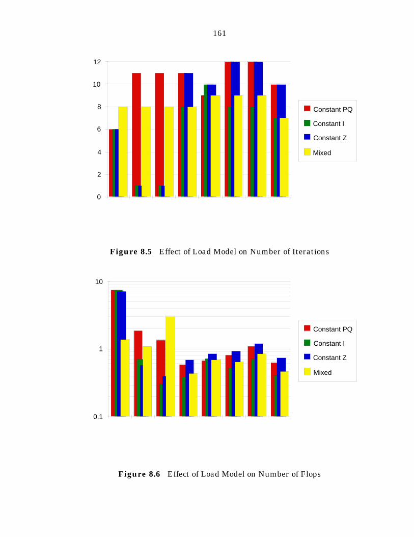
161

Figure 8.5 Effect of Load Model on Number of Iterations

Figure 8.6 Effect of Load Model on Number of Flops

0

2

4

6

8

10

12

Constant PQ

Constant I

Constant Z

Mixed

0.1

1

10

Constant PQ

Constant I

Constant Z

Mixed

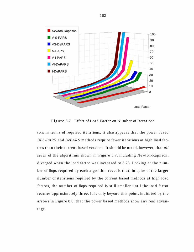
162

tors in terms of required iterations. It also appears that the power based

BFS-PARS and DePARS methods require fewer iterations at high load fac-

tors than their current based versions. It should be noted, however, that all

seven of the algorithms shown in Figure 8.7, including Newton-Raphson,

diverged when the load factor was increased to 3.75. Looking at the num-

ber of flops required by each algorithm reveals that, in spite of the larger

number of iterations required by the current based methods at high load

factors, the number of flops required is still smaller until the load factor

reaches approximately three. It is only beyond this point, indicated by the

arrows in Figure 8.8, that the power based methods show any real advan-

tage.

Figure 8.7 Effect of Load Factor on Number of Iterations

Load Factor

0

10

20

30

40

50

60

70

80

90

100Newton-Raphson

V-S-PARS

VS-DePARS

N-PARS

V-I-PARS

VI-DePARS

I-DePARS

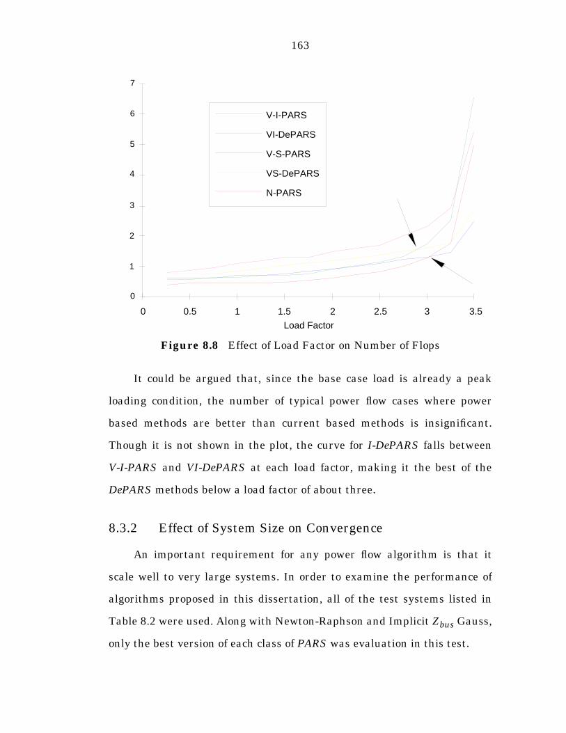
163

It could be argued that, since the base case load is already a peak

loading condition, the number of typical power flow cases where power

based methods are better than current based methods is insignificant.

Though it is not shown in the plot, the curve for I-DePARS falls between

V-I-PARS and VI-DePARS at each load factor, making it the best of the

DePARS methods below a load factor of about three.

8.3.2 Effect of System Size on Convergence

An important requirement for any power flow algorithm is that it

scale well to very large systems. In order to examine the performance of

algorithms proposed in this dissertation, all of the test systems listed in

Table 8.2 were used. Along with Newton-Raphson and Implicit Zbus Gauss,

only the best version of each class of PARS was evaluation in this test.

Figure 8.8 Effect of Load Factor on Number of Flops

Load Factor

0

1

2

3

4

5

6

7

0 0.5 1 1.5 2 2.5 3 3.5

V-I-PARS

VI-DePARS

V-S-PARS

VS-DePARS

N-PARS

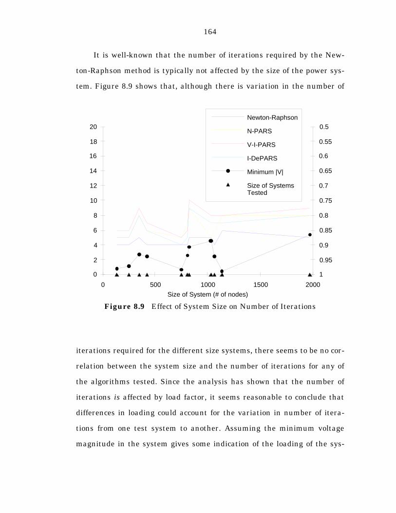
164

It is well-known that the number of iterations required by the New-

ton-Raphson method is typically not affected by the size of the power sys-

tem. Figure 8.9 shows that, although there is variation in the number of

iterations required for the different size systems, there seems to be no cor-

relation between the system size and the number of iterations for any of

the algorithms tested. Since the analysis has shown that the number of

iterations is affected by load factor, it seems reasonable to conclude that

differences in loading could account for the variation in number of itera-

tions from one test system to another. Assuming the minimum voltage

magnitude in the system gives some indication of the loading of the sys-

Figure 8.9 Effect of System Size on Number of Iterations

Size of System (# of nodes)

0

2

4

6

8

10

12

14

16

18

20

0 500 1000 1500 2000

0.5

0.55

0.6

0.65

0.7

0.75

0.8

0.85

0.9

0.95

1

Newton-Raphson

N-PARS

V-I-PARS

I-DePARS

Minimum |V|

Size of SystemsTested

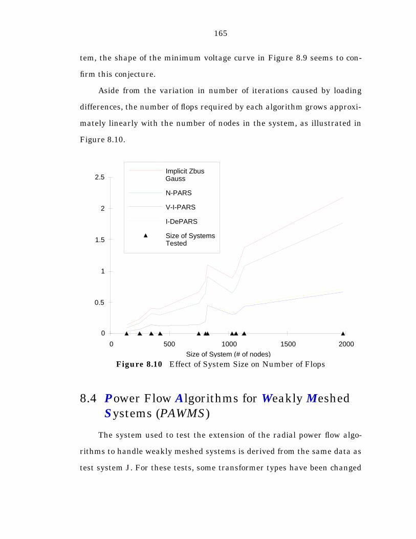
165

tem, the shape of the minimum voltage curve in Figure 8.9 seems to con-

firm this conjecture.

Aside from the variation in number of iterations caused by loading

differences, the number of flops required by each algorithm grows approxi-

mately linearly with the number of nodes in the system, as illustrated in

Figure 8.10.

8.4 Power Flow Algorithms for Weakly Meshed Systems (PAWMS)

The system used to test the extension of the radial power flow algo-

rithms to handle weakly meshed systems is derived from the same data as

test system J. For these tests, some transformer types have been changed

Figure 8.10 Effect of System Size on Number of FlopsSize of System (# of nodes)

0

0.5

1

1.5

2

2.5

0 500 1000 1500 2000

Implicit ZbusGauss

N-PARS

V-I-PARS

I-DePARS

Size of SystemsTested

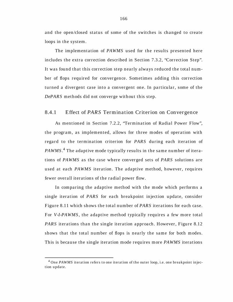
166

and the open/closed status of some of the switches is changed to create

loops in the system.

The implementation of PAWMS used for the results presented here

includes the extra correction described in Section 7.3.2, “Correction Step”.

It was found that this correction step nearly always reduced the total num-

ber of flops required for convergence. Sometimes adding this correction

turned a divergent case into a convergent one. In particular, some of the

DePARS methods did not converge without this step.

8.4.1 Effect of PARS Termination Criterion on Convergence

As mentioned in Section 7.2.2, “Termination of Radial Power Flow”,

the program, as implemented, allows for three modes of operation with

regard to the termination criterion for PARS during each iteration of

PAWMS.4 The adaptive mode typically results in the same number of itera-

tions of PAWMS as the case where converged sets of PARS solutions are

used at each PAWMS iteration. The adaptive method, however, requires

fewer overall iterations of the radial power flow.

In comparing the adaptive method with the mode which performs a

single iteration of PARS for each breakpoint injection update, consider

Figure 8.11 which shows the total number of PARS iterations for each case.

For V-I-PAWMS, the adaptive method typically requires a few more total

PARS iterations than the single iteration approach. However, Figure 8.12

shows that the total number of flops is nearly the same for both modes.

This is because the single iteration mode requires more PAWMS iterations

4 One PAWMS iteration refers to one iteration of the outer loop, i.e. one breakpoint injec-tion update.

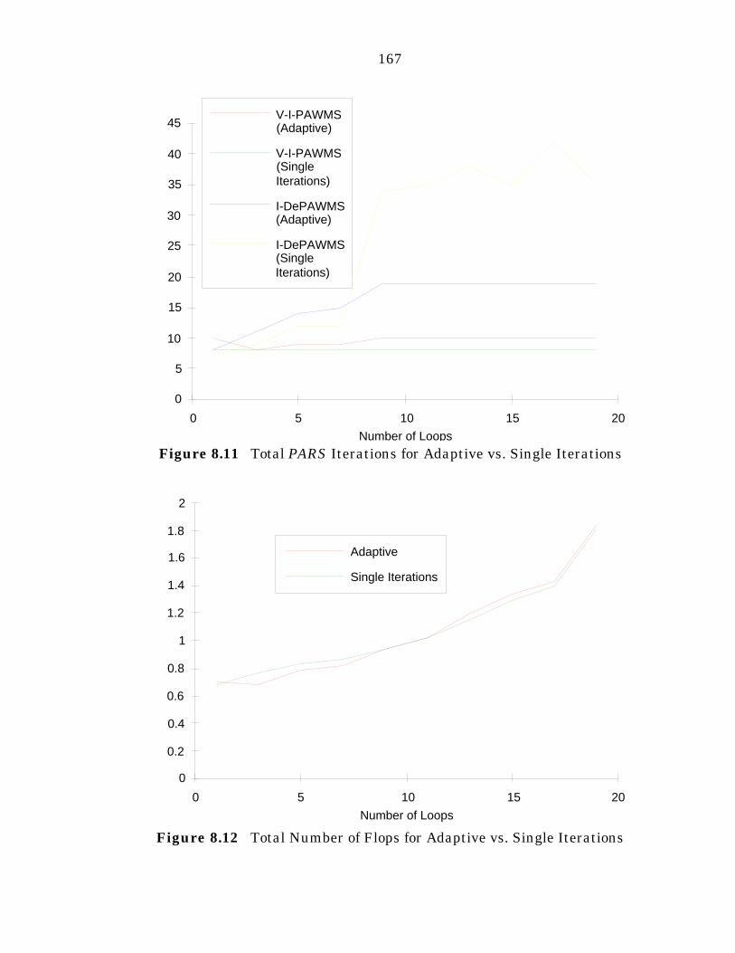
167

Figure 8.11 Total PARS Iterations for Adaptive vs. Single Iterations

Figure 8.12 Total Number of Flops for Adaptive vs. Single Iterations

Number of Loops

0

5

10

15

20

25

30

35

40

45

0 5 10 15 20

V-I-PAWMS(Adaptive)

V-I-PAWMS(SingleIterations)

I-DePAWMS(Adaptive)

I-DePAWMS(SingleIterations)

Number of Loops

0

0.2

0.4

0.6

0.8

1

1.2

1.4

1.6

1.8

2

0 5 10 15 20

Adaptive

Single Iterations

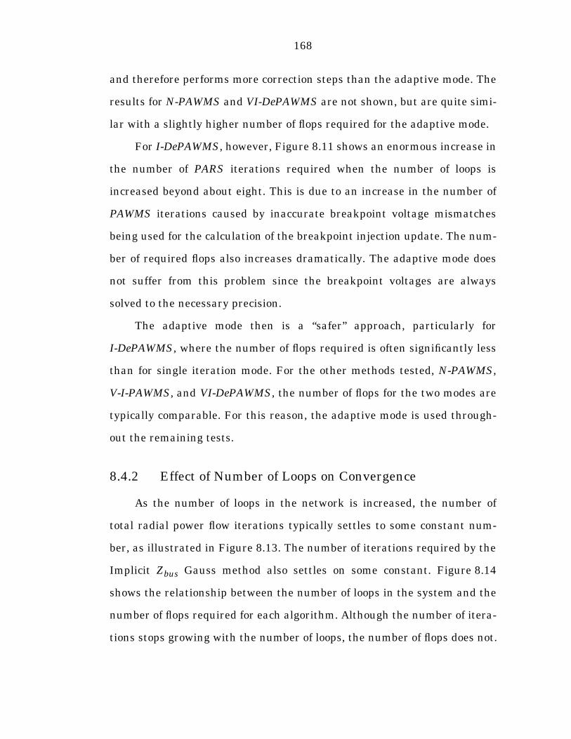
168

and therefore performs more correction steps than the adaptive mode. The

results for N-PAWMS and VI-DePAWMS are not shown, but are quite simi-

lar with a slightly higher number of flops required for the adaptive mode.

For I-DePAWMS, however, Figure 8.11 shows an enormous increase in

the number of PARS iterations required when the number of loops is

increased beyond about eight. This is due to an increase in the number of

PAWMS iterations caused by inaccurate breakpoint voltage mismatches

being used for the calculation of the breakpoint injection update. The num-

ber of required flops also increases dramatically. The adaptive mode does

not suffer from this problem since the breakpoint voltages are always

solved to the necessary precision.

The adaptive mode then is a “safer” approach, particularly for

I-DePAWMS, where the number of flops required is often significantly less

than for single iteration mode. For the other methods tested, N-PAWMS,

V-I-PAWMS, and VI-DePAWMS, the number of flops for the two modes are

typically comparable. For this reason, the adaptive mode is used through-

out the remaining tests.

8.4.2 Effect of Number of Loops on Convergence

As the number of loops in the network is increased, the number of

total radial power flow iterations typically settles to some constant num-

ber, as illustrated in Figure 8.13. The number of iterations required by the

Implicit Zbus Gauss method also settles on some constant. Figure 8.14

shows the relationship between the number of loops in the system and the

number of flops required for each algorithm. Although the number of itera-

tions stops growing with the number of loops, the number of flops does not.

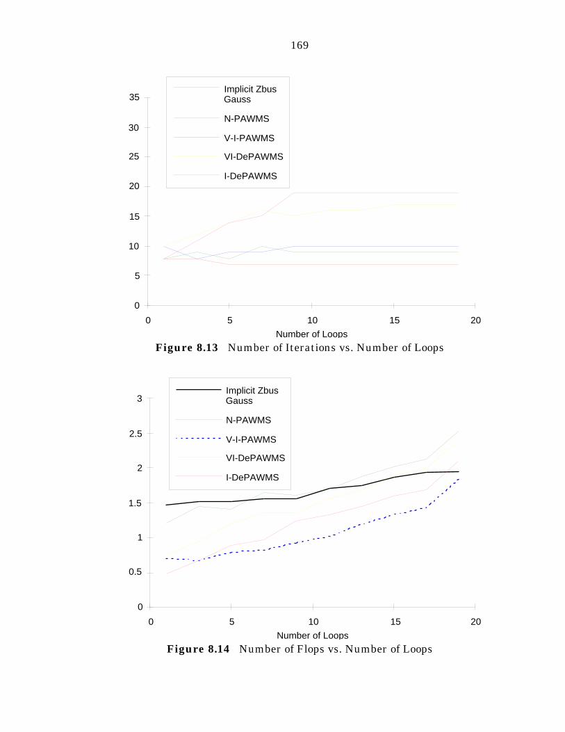
169

Figure 8.13 Number of Iterations vs. Number of Loops

Figure 8.14 Number of Flops vs. Number of Loops

Number of Loops

0

5

10

15

20

25

30

35

0 5 10 15 20

Implicit ZbusGauss

N-PAWMS

V-I-PAWMS

VI-DePAWMS

I-DePAWMS

Number of Loops

0

0.5

1

1.5

2

2.5

3

0 5 10 15 20

Implicit ZbusGauss

N-PAWMS

V-I-PAWMS

VI-DePAWMS

I-DePAWMS

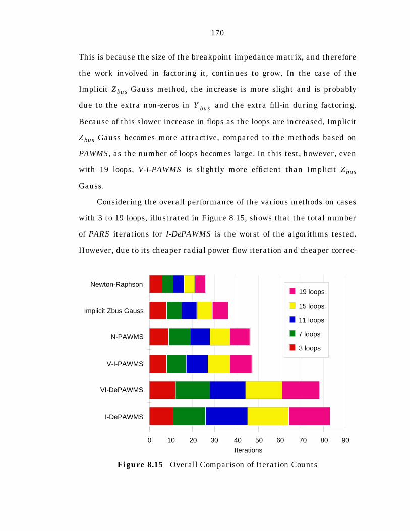
170

This is because the size of the breakpoint impedance matrix, and therefore

the work involved in factoring it, continues to grow. In the case of the

Implicit Zbus Gauss method, the increase is more slight and is probably

due to the extra non-zeros in and the extra fill-in during factoring.

Because of this slower increase in flops as the loops are increased, Implicit

Zbus Gauss becomes more attractive, compared to the methods based on

PAWMS, as the number of loops becomes large. In this test, however, even

with 19 loops, V-I-PAWMS is slightly more efficient than Implicit Zbus

Gauss.

Considering the overall performance of the various methods on cases

with 3 to 19 loops, illustrated in Figure 8.15, shows that the total number

of PARS iterations for I-DePAWMS is the worst of the algorithms tested.

However, due to its cheaper radial power flow iteration and cheaper correc-

Figure 8.15 Overall Comparison of Iteration Counts

Ybus

Iterations

0 10 20 30 40 50 60 70 80 90

Newton-Raphson

Implicit Zbus Gauss

N-PAWMS

V-I-PAWMS

VI-DePAWMS

I-DePAWMS

19 loops

15 loops

11 loops

7 loops

3 loops

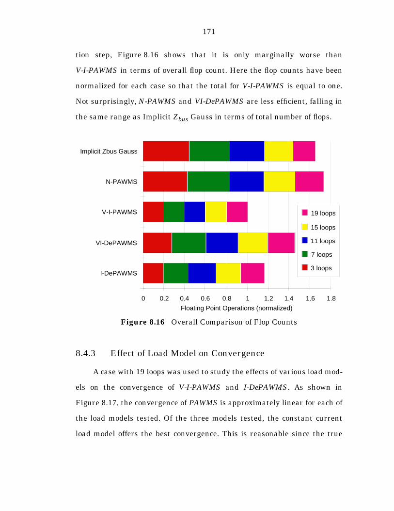
171

tion step, Figure 8.16 shows that it is only marginally worse than

V-I-PAWMS in terms of overall flop count. Here the flop counts have been

normalized for each case so that the total for V-I-PAWMS is equal to one.

Not surprisingly, N-PAWMS and VI-DePAWMS are less efficient, falling in

the same range as Implicit Zbus Gauss in terms of total number of flops.

8.4.3 Effect of Load Model on Convergence

A case with 19 loops was used to study the effects of various load mod-

els on the convergence of V-I-PAWMS and I-DePAWMS. As shown in

Figure 8.17, the convergence of PAWMS is approximately linear for each of

the load models tested. Of the three models tested, the constant current

load model offers the best convergence. This is reasonable since the true

Figure 8.16 Overall Comparison of Flop Counts

Floating Point Operations (normalized)

0 0.2 0.4 0.6 0.8 1 1.2 1.4 1.6 1.8

Implicit Zbus Gauss

N-PAWMS

V-I-PAWMS

VI-DePAWMS

I-DePAWMS

19 loops

15 loops

11 loops

7 loops

3 loops

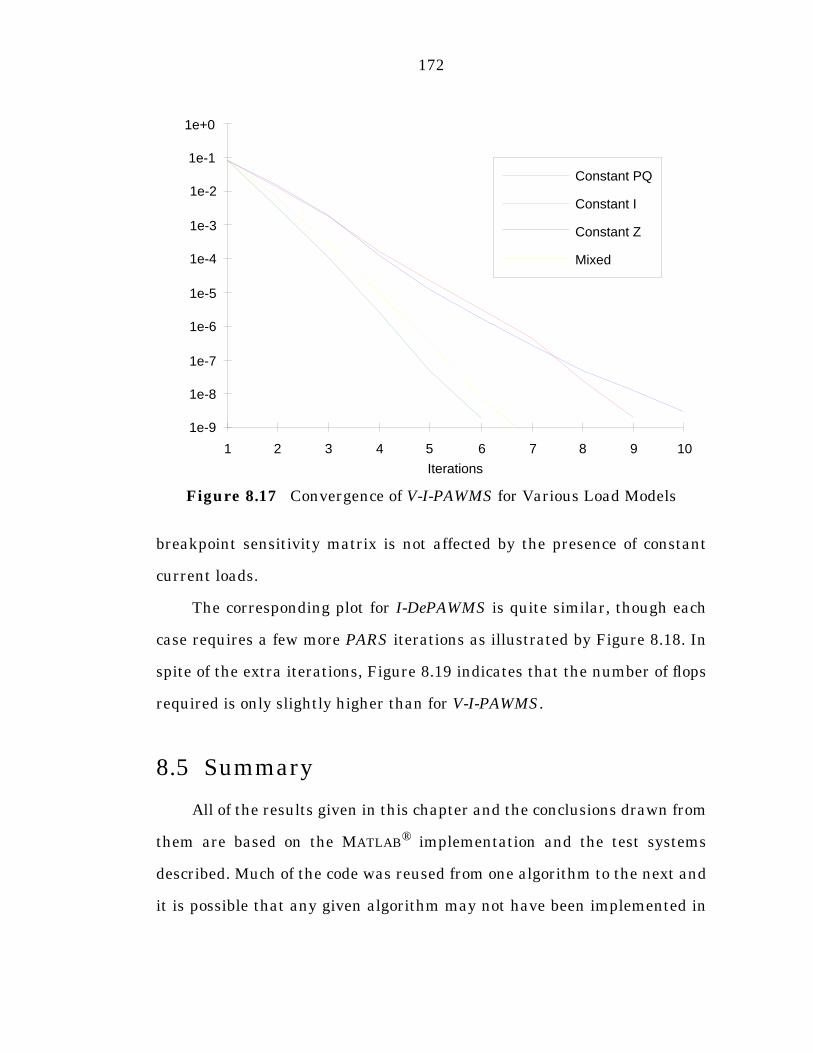
172

breakpoint sensitivity matrix is not affected by the presence of constant

current loads.

The corresponding plot for I-DePAWMS is quite similar, though each

case requires a few more PARS iterations as illustrated by Figure 8.18. In

spite of the extra iterations, Figure 8.19 indicates that the number of flops

required is only slightly higher than for V-I-PAWMS.

8.5 Summary

All of the results given in this chapter and the conclusions drawn from

them are based on the MATLAB® implementation and the test systems

described. Much of the code was reused from one algorithm to the next and

it is possible that any given algorithm may not have been implemented in

Figure 8.17 Convergence of V-I-PAWMS for Various Load Models

Iterations

1e-9

1e-8

1e-7

1e-6

1e-5

1e-4

1e-3

1e-2

1e-1

1e+0

1 2 3 4 5 6 7 8 9 10

Constant PQ

Constant I

Constant Z

Mixed

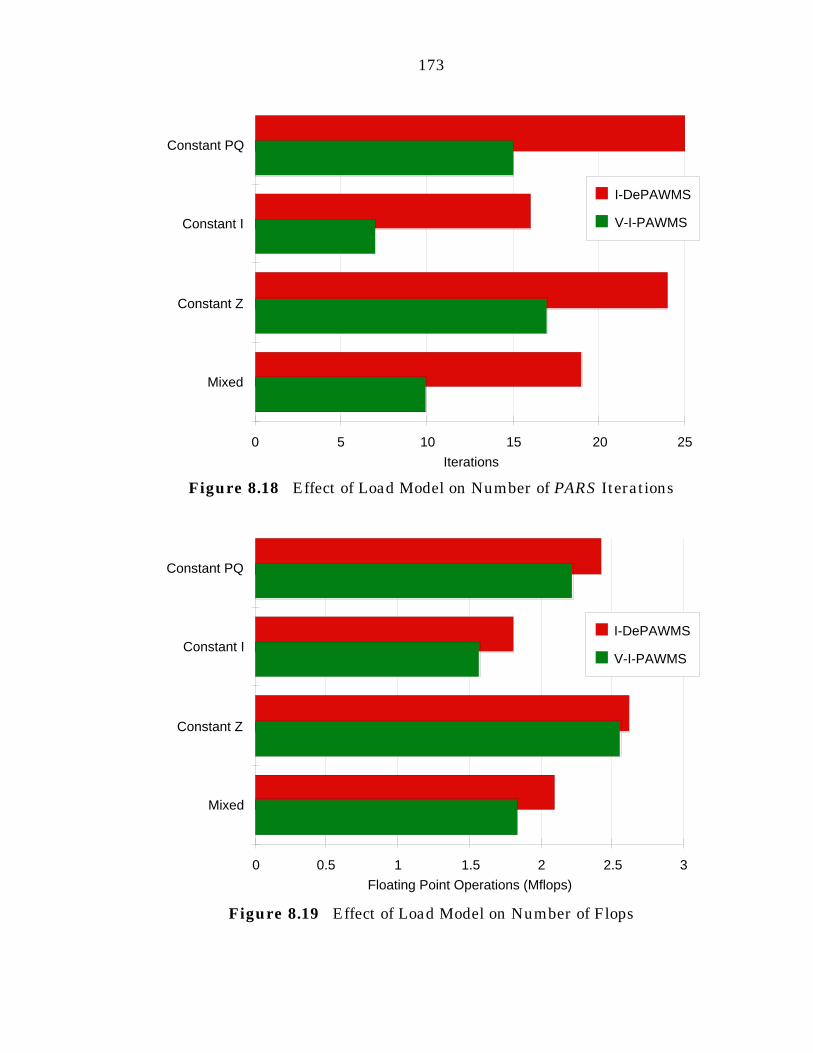
173

Figure 8.18 Effect of Load Model on Number of PARS Iterations

Figure 8.19 Effect of Load Model on Number of Flops

Iterations

0 5 10 15 20 25

Constant PQ

Constant I

Constant Z

Mixed

I-DePAWMS

V-I-PAWMS

Floating Point Operations (Mflops)

0 0.5 1 1.5 2 2.5 3

Constant PQ

Constant I

Constant Z

Mixed

I-DePAWMS

V-I-PAWMS

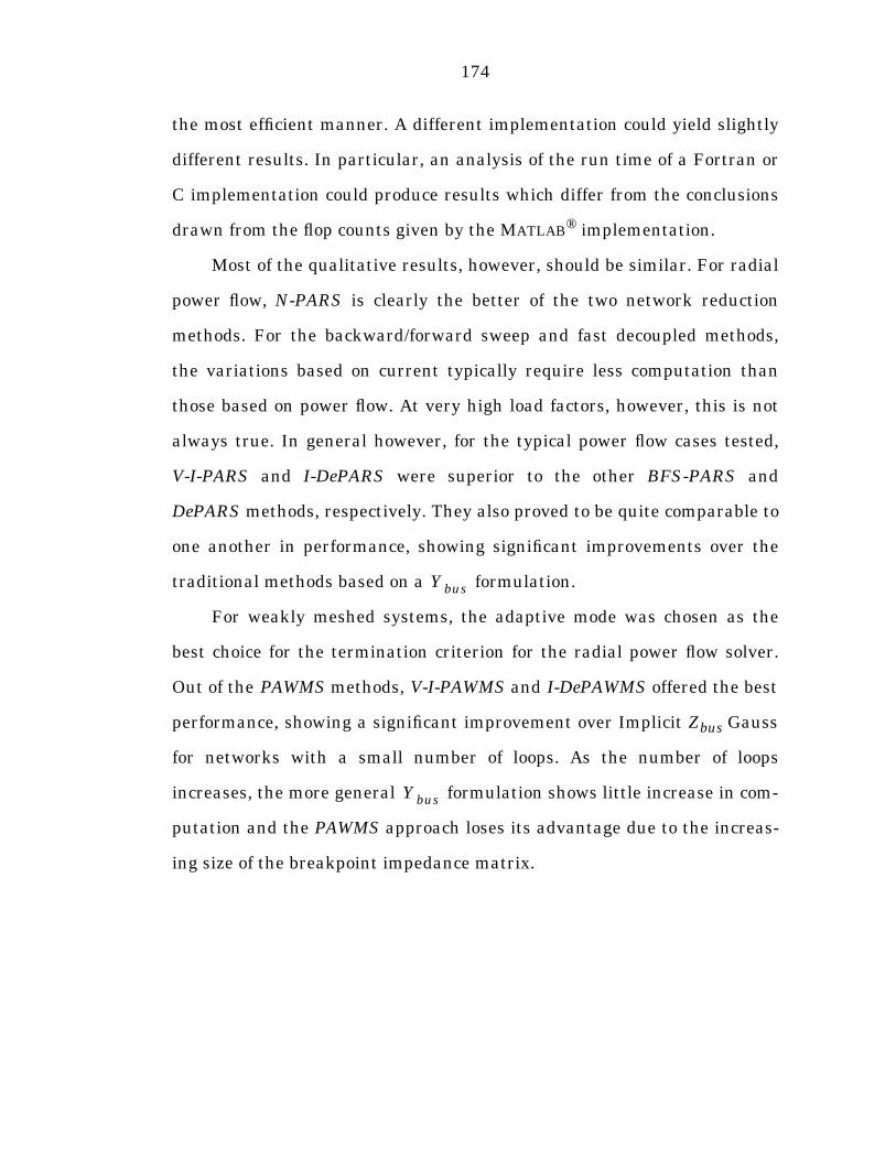
174

the most efficient manner. A different implementation could yield slightly

different results. In particular, an analysis of the run time of a Fortran or

C implementation could produce results which differ from the conclusions

drawn from the flop counts given by the MATLAB® implementation.

Most of the qualitative results, however, should be similar. For radial

power flow, N-PARS is clearly the better of the two network reduction

methods. For the backward/forward sweep and fast decoupled methods,

the variations based on current typically require less computation than

those based on power flow. At very high load factors, however, this is not

always true. In general however, for the typical power flow cases tested,

V-I-PARS and I-DePARS were superior to the other BFS-PARS and

DePARS methods, respectively. They also proved to be quite comparable to

one another in performance, showing significant improvements over the

traditional methods based on a formulation.

For weakly meshed systems, the adaptive mode was chosen as the

best choice for the termination criterion for the radial power flow solver.

Out of the PAWMS methods, V-I-PAWMS and I-DePAWMS offered the best

performance, showing a significant improvement over Implicit Zbus Gauss

for networks with a small number of loops. As the number of loops

increases, the more general formulation shows little increase in com-

putation and the PAWMS approach loses its advantage due to the increas-

ing size of the breakpoint impedance matrix.

Ybus

Ybus

175

Chapter 9

Conclusions

The objective of this work was to develop a comprehensive formula-

tion and an efficient solution algorithm for the distribution power flow

problem which takes into account the detailed and extensive modeling nec-

essary for use in the distribution automation environment of a real world

power system. This objective was achieved through extensions and gener-

alizations of existing power flow algorithms as well as through the develop-

ment of new methods.

9.1 Contributions

A general framework was developed which encompasses existing

radial power flow algorithms. This framework consists of the three main

classes of algorithms summarized in Table 9.1. Within each class, the

existing methods were generalized and extended to include more compre-

hensive modeling, and new algorithms for each class were introduced.

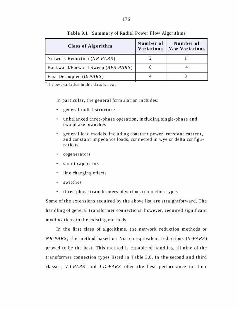
176

In particular, the general formulation includes:

• general radial structure

• unbalanced three-phase operation, including single-phase and two-phase branches

• general load models, including constant power, constant current, and constant impedance loads, connected in wye or delta configu-rations

• cogenerators

• shunt capacitors

• line charging effects

• switches

• three-phase transformers of various connection types

Some of the extensions required by the above list are straightforward. The

handling of general transformer connections, however, required significant

modifications to the existing methods.

In the first class of algorithms, the network reduction methods or

NR-PARS, the method based on Norton equivalent reductions (N-PARS)

proved to be the best. This method is capable of handling all nine of the

transformer connection types listed in Table 3.8. In the second and third

classes, V-I-PARS and I-DePARS offer the best performance in their

†The best variation in this class is new.

Table 9.1 Summary of Radial Power Flow Algorithms

Class of AlgorithmNumber ofVariations

Number of New Variations

Network Reduction (NR-PARS) 2 1†

Backward/Forward Sweep (BFS-PARS) 8 4

Fast Decoupled (DePARS) 4 3†

177

respective classes and have very similar computational requirements

which are significantly less than those of N-PARS. Both V-I-PARS and

I-DePARS, however, are restricted to systems which do not have any type 4

ungrounded wye to grounded wye transformer connections.

All three methods, N-PARS, V-I-PARS, and I-DePARS, require signifi-

cantly less computation than the traditional Newton-Raphson or Implicit

Zbus Gauss methods. Proofs of convergence have been given for the back-

ward/forward sweep and fast decoupled algorithms, indicating that they

are locally and linearly convergent. Furthermore, the simulation results

indicate that the number of iterations required for convergence is not a

function of the system size. Therefore, since the amount of work for each

iteration is proportional to the size of the system, the computational bur-

den of each algorithm grows only linearly with the size of the system, mak-

ing them suitable for very large distribution systems.

In order to solve weakly meshed systems, various extensions were

also made to the compensation method, previously applied only in conjunc-

tion with various backward/forward sweep methods. The general structure

proposed, with certain modeling restrictions, includes the following contri-

butions:

• general three-phase radial power flow

• general correction step

• secondary sources

• three-phase PV buses

• adaptive mode of radial power flow termination

178

Out of the PAWMS methods, V-I-PAWMS and I-DePAWMS offer the best

performance, showing a significant improvement over Implicit Zbus Gauss

for networks with a small number of loops.

9.2 Future Work

As with any work of research, there is always more that can be done.

Aside from further testing of the code and the algorithms as they stand,

there are several extensions and modifications which can be explored.

These include:

• expand network modeling

• remove limitations on formulation

• explore possibilities for improved contingency analysis

• implement for industry use

Though the modeling presented in this dissertation is quite general,

there are certainly improvements that can be made. As monitoring devices

become cheaper, more detailed information will become available on the

behavior of the components of a distribution system. In particular, with

more data it may be possible to use more accurate load models which are

not combinations of constant power, constant current, and constant imped-

ance. The inclusion of core loss in the transformer models is also important

for some applications, but was not included in this formulation due to a

lack of verifiable data. The automatic tap changes of voltage regulators

might also be considered.

Further extensions to the formulation of PAWMS could be explored as

well. In particular, it may be possible to extend the current formulation to

179

remove the limitations discussed in Section 7.2.1, making it possible to

handle systems with a mixture of grounded and ungrounded sections.

One common use of a power flow algorithm is to study various possi-

ble contingencies to determine the most profitable configuration for the

operation of the network. In such an application, the contingencies are typ-

ically specified with respect to some base case. If the power flow solution

for the base case is known, it may not be necessary to run a complete power

flow for each contingency. It is possible that the concepts behind the pro-

posed algorithms could be applied to compute partial or approximate

power flow solutions for the contingencies, given the base case solution.

The exploration of this possibility might yield more efficient approaches to

contingency analysis in distribution systems.

One of the most obvious ways of building upon the work presented in

this dissertation is to convert the MATLAB® program, used for the study of

the algorithms, to a compiled C or C++ program suitable for everyday use

in by a power engineer in industry. Such a program could be a very useful

tool for many applications in distribution planning and operation.

180

BIBLIOGRAPHY

[1] J. Arrillaga and C. P. Arnold, Computer Analysis of Power Systems,John Wiley & Sons, 1990.

[2] J. Arrillaga, C. P. Arnold, and B. J. Harker, Computer Modelling ofElectrical Power Systems, John Wiley & Sons, 1983.

[3] M. E. Baran and F. F. Wu, “Optimal Sizing of Capacitors Placed on aRadial Distribution System”, IEEE Transactions on Power Delivery,Vol. 4, No. 1, January 1989, pp. 735-742.

[4] R. Berg, Jr., E. S. Hawkins, and W. W. Pleines, “MechanizedCalculation of Unbalanced Load Flow on Radial DistributionCircuits”, IEEE Transactions on Power Apparatus and Systems,Vol. PAS-86, No. 4, April 1967, pp. 415-421.

[5] A. R. Bergen, Power Systems Analysis, Prentice-Hall, EnglewoodCliffs, NJ, 1986.

[6] H. E. Brown, G. K. Carter, H. H. Happ, C. E. Person, “Power FlowSolution by Impedance Matrix Iterative Method”, IEEE Transactionson Power Apparatus and Systems, Vol. PAS-82, April 1963, pp. 1-10.

[7] H. E. Brown, G. K. Carter, H. H. Happ, C. E. Person, “Z-MatrixAlgorithms in Load-Flow Programs”, IEEE Transactions on PowerApparatus and Systems, Vol. PAS-87, No. 3, March 1968, pp. 807-814.

[8] M. S. Chen and W. E. Dillon, “Power System Modeling”, Proceedingsof the IEEE, Vol. 62, No. 7, July 1974, pp. 901-915.

[9] T. H. Chen, M. S. Chen, K. J. Hwang, P. Kotas, and E. Chebli,“Distribution System Power Flow Analysis - A Rigid Approach”, IEEETransactions on Power Delivery, Vol. 6, No. 3, July 1991, pp. 1146-1152.

[10] T. H. Chen, “Generalized Distribution Analysis System”, Ph.D.Dissertation, The University of Texas at Arlington, May 1990.

[11] C. S. Cheng and D. Shirmohammadi, “A Three-Phase Power FlowMethod for Real-Time Distribution System Analysis”, IEEE/PES1994 Summer Meeting, San Francisco, CA, July 1994,94 SM 603-1 PWRS.

181

[12] H. D. Chiang, “A Decoupled Load Flow Method for Distribution PowerNetworks: Algorithms, Analysis and Convergence Study”, ElectricalPower & Energy Systems, Vol. 13, No. 3, June 1991, pp. 130-138.

[13] H. D. Chiang and M. E. Baran, “On the Existence and Uniqueness ofLoad Flow Solution for Radial Distribution Power Networks”, IEEETransactions on Circuits and Systems, Vol. 37, No. 3, March 1990,pp. 410-416.

[14] R. S. Dembo, S. C. Eisenstat, and T. Steihaug, “Inexact NewtonMethods”, SIAM Journal on Numerical Analysis, Vol. 19, No. 2, April1982, pp. 400-408.

[15] G. H. Golub and C. F. Van Loan, Matrix Computations, The JohnsHopkins University Press, Baltimore, MD, 1989.

[16] S. Iwamoto and Y. Tamura, “A Load Flow Calculation Method for Ill-Conditioned Power Systems”, IEEE Transactions on Power Apparatusand Systems, Vol. PAS-100, No. 4, April 1981, pp. 1736-1743.

[17] W. H. Kersting and D. L. Mendive, “An Application of Ladder NetworkTheory to the Solution of Three-Phase Radial Load-Flow Problems”,IEEE/PES 1976 Winter Meeting, New York, NY, January 1976,A 76 044-8.

[18] W. H. Kersting and W. H. Phillips, “A Radial Three-phase Power FlowProgram for the PC”, Conference paper, presented at 1987 FrontiersPower Conference, Stillwater, OK, October 1987.

[19] G.X. Luo and A. Semlyen, “Efficient Load Flow for Large WeaklyMeshed Networks”, IEEE Transactions on Power Systems, Vol. 5,No. 4, November 1990, pp. 1309-1316.

[20] D. Raji i , R. A kovski, R. Taleski, “Voltage Correction Power Flow”,IEEE/PES 1993 Summer Meeting, Vancouver, B.C., Canada, July1993, 93 SM 570-2.

[21] D. Raji i and A. Bose, “A Modification to the Fast Decoupled PowerFlow for Networks with High R/X Ratios”, IEEE Transactions onPower Systems, Vol. 3, No. 2, May 1988, pp. 743-746.

[22] R. Sedgewick, Algorithms, Addison-Wesley Publishing Company, Inc.,1983.

c c c

c c

182

[23] D. Shirmohammadi, H. W. Hong, A. Semlyen, and G. X. Luo, “ACompensation-based Power Flow Method for Weakly MeshedDistribution and Transmission Networks”, IEEE Transactions onPower Systems, Vol. 3, No. 2, May 1988, pp. 753-762.

[24] G. W. Stagg and A. H. El-Abiad, Computer Methods in Power SystemAnalysis, New York: McGraw Hill, 1968.

[25] B. Stott, “Review of Load-Flow Calculation Methods”, Proceedings ofthe IEEE, Vol. 62, No. 7, July 1974, pp. 916-929.

[26] B. Stott and O. Alsaç, “Fast Decoupled Load Flow”, IEEETransactions on Power Apparatus and Systems, Vol. PAS-93, May/June 1974, pp. 859-869.

[27] D. I. H. Sun, S. Abe, R. R. Shoults, M. S. Chen, P. Eichenberger, andD. Farris, “Calculation of Energy Losses in a Distribution System”,IEEE Transactions on Power Apparatus and Systems, Vol. PAS-99,No. 4, July/August 1980, pp. 1347-1356.

[28] W. F. Tinney and C. E. Hart, “Power Flow Solution by Newton’sMethod”, IEEE Transactions on Power Apparatus and Systems,Vol. PAS-86, No. 11, November 1967, pp. 1449-1460.

[29] W. F. Tinney and J. W. Walker, “Direct Solutions of Sparse NetworkEquations by Optimally Ordered Triangular Factorization”,Proceedings of the IEEE, Vol. 55, No. 11, November 1967, pp. 1801-1809.

[30] W. F. Tinney, “Compensation Methods for Network Solutions byOptimally Ordered Triangular Factorization”, Proceedings of thePICA Conference, Boston, MA, May 24-26, 1971, pp. 123-127.

[31] S. C. Tripathy, G. D. Prasad, O. P. Malik, and G. S. Hope, “Load FlowSolutions for Ill-Conditioned Power Systems by a Newton-LikeMethod”, IEEE Transactions on Power Apparatus and Systems,Vol. PAS-101, No. 10, October 1982, pp. 3648-3657.

[32] R. D. Zimmerman and H. D. Chiang, “Fast Decoupled Power Flow forUnbalanced Radial Distribution Systems”, IEEE/PES 1995 WinterMeeting, New York, NY, January 1995, 95 WM 219-6 PWRS.

COMPREHENSIVE D P F MODELING, FORMULATION, SOLUTION ALGORITHMS AND ANALYSIS · ·...

Documents

Transcript of COMPREHENSIVE D P F MODELING, FORMULATION, SOLUTION ALGORITHMS AND ANALYSIS · ·...