Compositional Model for Predicting Multilayer …lspCompositional Model for Predicting Multilayer...
169
Compositional Model for Predicting Multilayer Reflectances and Transmittances in Color Reproduction THÈSE Nº 3576 ( 2006 ) PRÉSENTÉE LE 14 JUIN 2006 À LA FACULTÉ INFORMATIQUE ET COMMUNICATIONS Laboratoire de systèmes périphériques SECTION D'INFORMATIQUE ÉCOLE POLYTECHNIQUE FÉDÉRALE DE LAUSANNE POUR L’OBTENTION DU GRADE DE DOCTEUR ÈS SCIENCES PAR Mathieu Hébert DEA image, Université Jean Monnet, Saint-Etienne, France de nationalité française acceptée sur proposition du jury : Prof. S. Süsstrunk, présidente du jury Prof. R. Hersch, directeur de thèse Prof. M. Elias, rapporteur Prof. J. Lafait, rapporteur Prof. L. Zuppiroli, rapporteur Lausanne, EPFL 2006
Transcript of Compositional Model for Predicting Multilayer …lspCompositional Model for Predicting Multilayer...

Compositional Model for Predicting Multilayer Reflectances and Transmittances in Color Reproduction
THÈSE Nº 3576 ( 2006 )
PRÉSENTÉE LE 14 JUIN 2006
À LA FACULTÉ INFORMATIQUE ET COMMUNICATIONS
Laboratoire de systèmes périphériques
SECTION D'INFORMATIQUE
ÉCOLE POLYTECHNIQUE FÉDÉRALE DE LAUSANNE
POUR L’OBTENTION DU GRADE DE DOCTEUR ÈS SCIENCES
PAR
Mathieu Hébert
DEA image, Université Jean Monnet, Saint-Etienne, France
de nationalité française
acceptée sur proposition du jury :
Prof. S. Süsstrunk, présidente du jury Prof. R. Hersch, directeur de thèse
Prof. M. Elias, rapporteur Prof. J. Lafait, rapporteur
Prof. L. Zuppiroli, rapporteur
Lausanne, EPFL 2006


i
Quoi qu’on fasse, on reconstruit toujours le monument à sa manière. Mais c’est déjà beaucoup
de n’employer que des pierres authentiques.
Marguerite Yourcenar, Carnets de notes de “Mémoires d’Hadrien”

ii

iii
Acknowledgements
First of all, I would like to express my gratitude to Prof. Roger D. Hersch, director of my research program. Despite the distance between Lausanne and Lyon, he continuously sustained and supervised my work. I thank him for trusting in my capacities and for the pertinence of his advice. It is also a pleasure to thank Prof. Jean-Marie Becker, who taught me so much about mathematics and pedagogy. Meeting him was a determining point in my life, and perhaps the reason for pursuing my carrier on a scientific track. I thank Prof. Jourlin for the opportunity of discovering the field of image and color process-ing and for the impetus he gave me for my career.
Many persons have contributed to the development of my research. I specially thank Lionel Simonot of the University of Poitiers and Patrick Emmel from Clariant for their interesting discussions. I am grateful to Eric Charron from the Laboratoire d’Optique des Solides in Paris, to Prof. Hartmut Schmidt from the University of Technology of Darm-stadt, to Prof. Plummer from the École Polytechnique Fédérale de Lausanne, and to Mr. Luc Choulet, for having generously accepted to give me some time and letting me benefit from their experience. Many thanks to my colleagues Matthieu, Isaac and Laurent, for their precious help and for spending together enjoyable time during these four years. I also thank Mrs. Moira Lanthelme for her help, and my friends, especially Jo, Mathias, Siegfried, Nico and Broqui, for their interest in my work and their nonscientific or artistic point of view.
I would like to finish by expressing my gratitude to my family: my parents and my brother for their constant encouragement, and of course my wife, Valou, who has brought me poetry at times when it is lacking in technical science, and revealed me, day in, day out, a colorful world which I would not know without her.

iv

v
Abstract
The color of materials such as paints, prints and glass may be characterized by a reflec-tance or a transmittance spectrum. Modeling their reflectance and their transmittance requires describing the interaction of light, from the light source to the observer, across the different layers and interfaces. Each layer and interface behaves as a light reflector and transmitter, and is given the generic name of “biface”. Multilayer specimens, called “multifaces”, result from the superposition of various bifaces between which light is sub-ject to multiple reflections and transmissions.
We establish a multiple reflection-transmission model which describes the transfers of fluxes between the different bifaces using the basic laws of geometrical optics. This ap-proach is valid for multilayer specimen composed of strongly scattering and/or nonscat-tering layers and flat interfaces. Weakly scattering layers and rough interfaces are allowed if they are surrounded by strongly scattering layers.
We first develop the multiple reflection-transmission model in a general manner, i.e. regardless to the specific optical properties of the bifaces. The light multiple reflection-transmission process is represented by a Markov chain. The well established mathematical tools provided by the Markov theory enable deriving the formulae for the reflectance and transmittance of superposed bifaces. Then, we show how the multiple reflection-transmission formulae are applied for a specific multiface and for a specific measuring geometry. We retrieve as special cases of our general model the Kubelka model for stacked intensely scattering layers, the Williams-Clapper model for a diffusing back-ground coated with a non-scattering layer, the Saunderson correction, and the Clapper-Yule model for high quality halftone prints. We finally explore new possibilities offered by the multiple reflection-transmission model, both for developing new reflectance or trans-mittance models and for checking the relevance of parameters deduced from measured data. We develop a method for characterizing papers independently of the measuring ge-ometry by modeling two superposed sheets of paper and draw the bases of a reflectance and transmittance prediction model for recto-verso halftone prints.
Keywords : Multilayer reflectance and transmittance, multiple reflections and transmis-sions, compositional spectral prediction model, Kubelka-Munk theory, Williams-Clapper model, Clapper-Yule model, Markov chains.

vi

vii
Résumé
La couleur de matériaux multicouches que l’on rencontre dans les peintures ou les im-primés peut être caractérisée par un spectre de réflectance ou de transmittance. Pour pré-dire de tels spectres, il est nécessaire de décrire l’interaction de la lumière avec les diffé-rents constituants du multicouche (couches et interfaces), de la source lumineuse à l’observateur. Chacun de ces constituants se comporte comme un réflecteur et un trans-metteur lumineux, auquel on donne le nom générique de “biface”. Dans les multicouches, “appelés multifaces”, la lumière est sujette à un phénomène de réflexion-transmission multiple entre les différents bifaces superposés.
Nous proposons un modèle de réflexion-transmission multiple où les transferts de flux entre bifaces sont établis d’après les lois de l’optique géométrique. Cette approche est valable pour des multicouches composés de couches fortement diffusantes, de couches non diffusantes, et d’interfaces planes. Elle reste valable avec des interfaces rugueuses et des couches faiblement diffusantes lorsque celles-ci sont directement bordées par des couches fortement diffusantes.
Nous développons d’abord le modèle général de réflexion-transmission multiple, sans spécifier la nature diffusante ou non des bifaces. Le processus de transfert lumineux est représenté par une chaîne de Markov. La théorie de Markov nous offre les outils mathé-matiques permettant d’obtenir efficacement les formules de réflectance et de transmit-tance du multicouche. Nous montrons ensuite comment la réflectance et la transmittance des faces doivent être spécifiées pour un multicouche et une géométrie de mesure donnés. Nous obtenons ainsi un modèle compositionnel valable pour tout type de multicouche correspondant à un multiface régulier. Le modèle de Kubelka, spécifique aux empilements de couches fortement diffusantes ayant toutes le même indice de réfraction, le modèle de Williams-Clapper, spécifique aux fonds diffusants couverts d’une couche transparente colorée, la correction de Saunderson, ainsi que le modèle de Clapper-Yule valable pour les imprimés en demi-ton à linéature élevée deviennent des cas particuliers de notre modèle compositionnel. Enfin, nous explorons quelques nouvelles possibilités offertes par notre modèle, tant pour prédire des réflectance et des transmittances de multicouches (papiers, imprimés), que pour vérifier des valeurs de spectre déduites de mesures (spectre de transmittance d’une encre, paramètres intrinsèques d’un papier). Nous établissons égale-ment les bases d’un modèle de prédiction spectral pour des échantillons imprimés en de-mi-tons à la fois sur le recto et sur le verso.
Mots-clés : Réflectance et transmittance multicouches, réflexions et transmissions multi-ples, modèle compositionnel de prédiction de spectres, théorie de Kubelka-Munk, modèle Williams-Clapper, modèle Clapper-Yule, chaînes de Markov.

viii

ix
Contents
Acknowledgments iii
Abstract v
Résumé vii
Contents ix
Introduction 1
Chapter 1. Reflectance and transmittance 5 1.1 Basic concepts of radiometry..................................................................................5
1.1.1 The four fundamental radiometric quantities ................................................5 1.1.2 Relation between irradiance and radiance .....................................................7 1.1.3 Radiance invariance .......................................................................................7 1.1.4 Lambert’s law ................................................................................................8
1.2 Definitions of reflectance and transmittance ..........................................................9 1.2.1 BRDF and BTDF ..........................................................................................9 1.2.2 Reflectance and transmittance.......................................................................9 1.2.3 Reflectance and transmittance factor...........................................................12
1.3 Measuring geometries ...........................................................................................12 1.3.1 Setups for reflectance and transmittance measurements..............................13 1.3.2 Measuring the BRDF...................................................................................14
Summary....................................................................................................................15
Chapter 2. Faces, bifaces, multifaces 17 2.1 Introduction .........................................................................................................17
2.1.1 Definitions....................................................................................................18 2.1.2 Hierarchical representation of multilayer specimens ....................................18
2.2 Faces ....................................................................................................................19 2.3 Bifaces ..................................................................................................................20 2.4 Multifaces .............................................................................................................21 Summary....................................................................................................................22
Chapter 3. Optical properties of transparent bifaces 25 3.1 Generalities on transparent bifaces ......................................................................25
3.1.1 Snell’s laws...................................................................................................25 3.1.2 Radiance invariance at a transparent face ...................................................27 3.1.3 Reflectance and transmittance of transparent bifaces..................................27
3.2 Flat interfaces ......................................................................................................28 3.2.1 Fresnel formulae ..........................................................................................28 3.2.2 Reflectance and transmittance of flat interfaces ..........................................30

x
3.3 Transparent layers ...............................................................................................32 3.3.1 Beer’s law.....................................................................................................32 3.3.2 Transmittance of a transparent layer ..........................................................32 3.3.3 Superposed transparent layers .....................................................................33
3.4 Transparent multifaces.........................................................................................33 3.4.1 Multiple reflection-transmission of polarized directional light .....................34 3.4.2 Directional reflectance and transmittance for polarized and natural light...36
Summary....................................................................................................................37
Chapter 4. Optical properties of scattering and Lambertian bifaces 39 4.1 Rough interfaces...................................................................................................39
4.1.1 Directional and Lambertian reflectances of rough interfaces .......................40 4.1.2 BRDF and BTDF models ............................................................................41
4.2 Scattering layers...................................................................................................44 4.2.1 Scattering parameters ..................................................................................44 4.2.2 Types of scattering.......................................................................................46 4.2.3 The radiative transfer equation ...................................................................46
4.3 Lambertian layers.................................................................................................47 4.3.1 Kubelka-Munk two-flux model.....................................................................48 4.3.2 Differential equation system ........................................................................48 4.3.3 Solutions for the differential equation system..............................................49 4.3.4 Intrinsic reflectance and transmittance of a Lambertian layer ....................50 4.3.5 Lambertian layer bordered by bifaces..........................................................51
Summary....................................................................................................................53
Chapter 5. Multiple reflection-transmission of light in multifaces 55 5.1 Light multiple reflection-transmission between bifaces ........................................55
5.1.1 Multiple reflection-transmission process ......................................................55 5.1.2 Example of the quadriface ...........................................................................57 5.1.3 Time-dependent and time-independent processes ........................................59
5.2 Regular multifaces................................................................................................60 5.2.1 Conditions of regularity ...............................................................................60 5.2.2 Representations of regular multifaces ..........................................................61 5.2.3 Analogy between regular multifaces and Markov chains .............................62
5.3 Compositional model for regular multifaces .........................................................64 5.3.1 The quadriface formula................................................................................64 5.3.2 The hexaface formula...................................................................................67 5.3.3 Associativity of the composition of bifaces ..................................................68 5.3.4 Composition formula for more than two bifaces ..........................................68
5.4 Biface splitting .....................................................................................................70 Summary....................................................................................................................71
Chapter 6. Reflectance and transmittance models 73 6.1 Elaboration of a reflectance and transmittance model .........................................73
6.1.1 Types of regular bifaces ...............................................................................73 6.1.2 Faces reflectances and transmittances in mixed multifaces .........................74
xi
6.1.3 Standard procedure for the development of a model ...................................75 6.2 Classical models for transparent and wholly-Lambertian multifaces....................77
6.2.1 Transparent multifaces ................................................................................77 6.2.2 Wholly-Lambertian multifaces (Kubelka’s model).......................................78
6.3 Transparent bifaces superposed to a Lambertian background .............................79 6.3.1 Background with an interface with air (Saunderson’s model) .....................79 6.3.2 Background coated by a transparent layer (Williams-Clapper model) ........81 6.3.3 Background and transparent layer having different refractive indices.........84
Summary....................................................................................................................86
Chapter 7. Compositional models for paper 87 7.1 Single paper sheet model ......................................................................................87
7.1.1 Global reflectance and transmittance of a paper sheet ................................88 7.1.2 Internal reflectance and transmittance of a paper sheet ..............................90 7.1.3 Relation with the Kubelka-Munk model ......................................................92 7.1.4 Deducing intrinsic parameters of paper from measurements .......................92
7.2 The double sheet model........................................................................................94 7.2.1 Model for a full contact between the sheets.................................................95 7.2.2 Model without contact between the sheets ..................................................95
7.3 Experimental results.............................................................................................99 Summary.................................................................................................................. 101
Chapter 8. Compositional models for prints 103 8.1 Ink transmittance............................................................................................... 103
8.1.1 Reflectance and transmittance of solid ink patches ................................... 103 8.1.2 Deducing ink transmittances from measurements...................................... 106
8.2 Halftone prints ................................................................................................... 107 8.2.1 Ideal halftone print .................................................................................... 107 8.2.2 Characterization of halftone inked layers................................................... 108 8.2.3 Validity of the compositional model with halftone prints.......................... 109
8.3 Reflectance models for halftone prints ............................................................... 111 8.3.1 Extended Williams-Clapper model for halftone prints............................... 111 8.3.2 Clapper-Yule model ................................................................................... 112 8.3.3 Deducing dot surface coverages of paper from measurements ................... 113 8.3.4 Prediction of multi-ink halftone prints ...................................................... 114
8.4 Reflectance and transmittance model for recto-verso halftone prints................. 114 8.4.1 Reflectance and transmittance model ........................................................ 115 8.4.2 Experimental verification........................................................................... 116
Summary.................................................................................................................. 117
Conclusion 119
Appendix A. Complements of radiometry 121 A.1 Relationship between reflectance and BRDF .................................................... 121 A.2 Reflectance and transmittance measured with a radiance detector................... 122 A.3 Cosine correction in measures of BRDFs .......................................................... 123

xii
Appendix B. Markov chains 127 B.1 Definition of a Markov chain............................................................................. 127 B.2 Probability transition matrices.......................................................................... 127 B.3 Properties of nonnegative, stochastic and substochastic matrices ..................... 129
B.3.1 Non-Negative matrices .............................................................................. 129 B.3.2 Stochastic and substochastic matrices....................................................... 129
B.4 Absorbing Markov chains .................................................................................. 132
Appendix C. Compositional formulae 135 C.1 Quadriface formula ............................................................................................ 135 C.2 Hexaface formula ............................................................................................... 137
Appendix D. Characterization of the external bifaces 139 D.1 Internal reflectance r ......................................................................................... 139 D.2 Penetration transmittance p.............................................................................. 140 D.3 Exit transmittance x.......................................................................................... 140 D.4 External reflectance s ........................................................................................ 142
References 145
Biography 149
Index 151
Frequently used formulae 155

1
Introduction
For thousands of years, the visual aspect of man-made objects has undergone multiple modifications due to the ingeniosity of craftmen and artists, creating new styles and satis-fying new clients. The increasing complexity of the crafmanship (and later on the indus-try) of potteries, ceramics, glasses, paintings and printing processes, etc. has been devel-oped on a basis of trial-and-error. In a very late stage, with geometrical optics in the 17th century and wave nature of light in the 19th century, a thorough understanding of these complex processes has taken place. It has appeared that the concept of “color” is very complex because it mixes three agents : light itself, matter and the human vision system [ZB03].
This practical complexity of the domain of color and the growing needs of industry in terms of quality and reproducibility explains that more or less ad hoc models have been proposed in a sporadic manner, for different classes of material. On the one side, physical models describe the changes of propagation and of spectrum that light undergoes when interacting induced with material objects. On the other side, psychophysical models study how the spectral image of objects carried by light is analyzed and interpreted by the hu-man visual system in terms of color, contrast [HV04], transparency [SIM02], gloss [OKV04], etc.
The present work focuses on the physical aspect of color, i.e. on the relationship be-tween light spectra considered respectively before and after reflection or transmission by an object, given by a reflectance or a transmittance spectrum. For predicting such spectra for a given multilayer object, it is necessary to describe the behavior of light in each layer and at each interface between the layers, which may extremely complex due to coexis-tence of multiple phenomena of reflection, refraction, scattering [Cha60, BS63], diffrac-tion, extinction or interference [BW99], generally dependent on the directionality and the polarization of light.
In order to simplify the multilayer reflectance and transmittance model, we consider only natural incident light, which is incoherent and unpolarized [BW99]. We also consider multilayers as being superpositions of layers and interfaces between these layers, each one being responsible of light reflection, transmission and possibly absorption. We assume that the reflectance and the transmittance of the different layers and interfaces can be determined independently, using for each one a specific model relying on geometrical op-tics: non-scattering layers may be characterized thanks to Beer’s law [Per95]; intensely scattering layers thanks to the Kubelka-Munk two-flux theory [KM31]; categories of weakly scattering layers thanks to a particular solution of the radiative transfer equation [Cha60]; flat interfaces thanks to Fresnel’s formulae [BW99] and rough interfaces with large roughness thanks to a microfacet model [TS67]. Thanks to the principle of conserva-tion of energy, absorption is considered as the complementary of reflection and transmis-sion. Multilayers containing layers or interfaces for which the wave nature of light should be explicitly taken into account are excluded from the present study. Non-scattering lay-ers are assumed to be thick enough for avoiding interference phenomena.
For predicting the reflectance and the transmittance of the multilayer specimens speci-

2 Introduction
fied above, we introduce a new modelization methodology which has been primarily de-veloped for paper and prints but may also be suitable for other multilayer objects, such as glass slices or photographs. In our approach, light interacting with colored objects consists of a collection of directed photons that are subject to reflection or transmission. Various models using this reflection/transmission basis have appeared in the 1950s. They concern complex materials, such as paper or pigmented coating, but use a reduced number of pa-rameters and a relatively simple mathematical development: Kubelka’s model [Kub54] expresses the reflectance and the transmittance of superposed intensely scattering layers as functions of the reflectance and the transmittance of each layer; Williams and Clapper [WC53] modeled the reflectance of a diffusing background coated with a non-scattering absorbing layer, as a function of the reflectance of the background and the transmittance of the non-scattering layer; Clapper and Yule [CY53] developed a model for halftone prints similar to the Williams-Clapper model, with some simplifications in the equations [HH04]. The accuracy of these models has been experimentally stated for the type of specimens that they concern. However, as a major drawback, they are not general enough for being simply extended to new types of colored supports. For instance, the Williams-Clapper model, initially developed for photographs, cannot be used anymore if one likes to protect a photograph with a tinted glaze. None of the models mentioned above enables considering such a multilayer comprising a paper sheet, a colored coating and a glass layer with an eventual air layer between them, all layers having reflecting and transmit-ting interfaces. One would have to develop a specific model for that special case [SHH06]. Furthermore, if one places behind the glaze a halftone print instead of a photograph, an-other specific model should be again developed. We thus see the practical interest that would provide a more general model where the optical phenomena of reflection and transmission would be described independently of the material.
Radiometry defines functions permitting to characterize illuminations, reflections and transmissions regardless of specified objects. We follow the same idea for multilayers, by describing light reflections and transmissions inside an abstract specimen composed of unspecified superposed elements. Every element able to reflect or/and transmit light, i.e. every layer and interface between layers, is represented by a single concept named “bi-face”. The adjacency of two bifaces and the mutual exchange of light between them due to multiple reflection-transmission are represented by the fundamental concept of “com-position” of bifaces. In a first step, the reflectance and the transmittance of the bifaces are characterized for its both sides (named “faces”). In a second step, a multiple reflec-tion-transmission model describes the transfers of fluxes between the faces contained in the multilayer specimen (named “multiface”). The obtained general expressions for reflec-tance and transmittance of multifaces are, in the most general case, irreducible infinite sums, but they can often be reduced to exact closed-form formulae. These formulae char-acterize the composition of bifaces and are by consequent called “composition formulae”.
Our compositional model aims at embodying all types of interfaces (flat, rough) and layers (transparent, weakly or intensely scattering). It should be capable of considering as well polished glass slices as matte paper sheets, in which light behaves in an extremely different manner. For the purpose of generality, we have created an appropriate formal-ism comprising: 1) a classification of the bifaces according to their light scattering proper-ties, 2) different well-defined types of reflectances and transmittances, 3) a graphical

Introduction 3
framework permitting to visualize the multiple reflection-transmission of light within mul-tifaces, 4) a notational framework including a matrix-like formulation for the composition of bifaces.
The notion of composition and the compositional formulae, as well as the conditions for their validity and the way for using them in special applications, are the main contri-bution of this thesis. The present dissertation is structured according to four parts, each one being composed of two chapters:
Part I (Chap. 1 and 2) − Basic definitions
Chapter 1 gives the definitions of reflectance and transmittance and presents briefly commonly used measuring devices. Chapter 2 gives the definitions of face, biface and mul-tiface, on which our formalism relies. Bifaces and multifaces are classified according to their scattering properties.
Part II (Chap. 3 and 4) − Optical properties of interfaces and layers
This second part presents the characteristics of bifaces, i.e. of interfaces and of layers. The different types of interfaces and of layers are presented in two chapters according to their scattering properties. Chapter 3 concerns flat interfaces and transparent layers (grouped into the concept of “transparent bifaces”), which have in common the property of being nonscattering. Chapter 4 deals with rough interfaces and scattering layers (“scat-tering bifaces”). Intensely scattering layers (“Lambertian bifaces”) are considered sepa-rately.
Part III (Chap. 5 and 6) − The compositional model
The compositional model is presented in two parts: in the first part (Chapter 5), the reflectance and transmittance formulae for multifaces (the “compositional formulae”) are established regardless to the nature of the bifaces. Then, in Chapter 6, we show how the reflectance and transmittance of each biface are specified, first in general, then in the spe-cial cases of multifaces considered in the existing models of Kubelka [Kub54], of Saunder-son [Sau42], of Williams and Clapper [WC53], of Shore and Spoonhower [SS00] and of Simonot, Hébert and Hersch [SHH06].
Part IV (Chap. 7 and 8) − Application of the compositional model to papers and prints
We apply our compositional model to papers, in Chapter 7, and to prints, in Chapter 8. We develop a method for characterizing papers independently of the measuring geome-try by modeling two superposed sheets of paper. We also compare the coherence between ink transmittances deduced from the measure of the reflectance and of the transmittance of monocolorant prints. Finally, we draw the bases of a reflectance and transmittance model for recto-verso halftone prints.

4 Introduction
Crown-shaped glossy coating deposited on a matte magenta flat tint. The surface reflection on top of the glossy area as well as the multiple reflections taking place beneath the air-coating interface are responsible of remarkable changes of color compared to the matte area (Front page of [Hel02], photograph by Siegfried Marque).

5
Chapter 1.
Reflectance and transmittance
Radiometry aims at characterizing rigorously the intuitive concepts of light quantity and spatial location, without having to consider specifically any type of material. In the present chapter, we first recall the four fundamental radiometric quantities: flux, irradiance, intensity and radiance (Sect. 1.1). They permit to characterize the two main phenomena of interest in our study, i.e. reflection and transmission. The frac-tions of incident light that are reflected and transmitted by the material are thus rep-resented by the reflectance and the transmittance (Sect. 1.2) whose definition necessi-tates specifying explicitly the conditions of illumination and the conditions of observa-tion. We define special types of reflectance and transmittance for the needs of the next chapters, called “directional” when the incident light comes from a single direc-tion, “diffuse” when it comes from the whole hemisphere with a nonhomogenous an-gular distribution, and “Lambertian” when it comes from the hemisphere with a ho-mogenous angular distribution. Finally, we propose a survey of common devices used for measuring reflectances and transmittances (Sect. 1.3).
1.1 Basic concepts of radiometry
Radiometry defines four fundamental quantities relative to radiations: radiant flux, irradiance, radiant intensity and radiance [McC94]. These quantities can be applied to light and can be measured in practice with instruments in laboratories.
We consider that incident light is natural, i.e. incoherent and unpolarized. Natural unpolarized light may be modeled by two independent and equal linearly polarized com-ponents [BW99]. The radiometric quantities may therefore be decoupled into these two components. There is no time-dependent behavior in the system, which excludes phospho-rescence1. The energy of different wavelengths is decoupled, i.e. the energy associated with a certain region of space or surface at wavelength λ1 is independent of the energy at wavelength λ2, which excludes phenomena of fluorescence2. Every radiometric quantity may therefore be a wavelength-dependent function.
1.1.1 The four fundamental radiometric quantities
Radiant flux Φ (or simply flux) is the energy flowing through a surface per unit time. Flux is expressed in watts.
⎯⎯⎯⎯⎯⎯⎯⎯⎯⎯⎯
1 Phosphorescence: Persistent emission of light following exposure to and removal of incident radiation. 2 Fluorescence: The emission of electromagnetic radiation stimulated in a substance by the absorption of incident radiation and persisting only as long as the stimulating radiation is continued.

6 Chapter 1
Sx
x dθ dA
dφ
dθθ
x sinθdφ
N
dω
flux element d 2Φ
ds
ds cosθ
θ
(a) (b)
Fig. 1.1: Geometry for the definitions of (a) solid angle and (b) radiance.
The solid angle dω subtended by area dA at point S is the ratio of the area dA of a portion of sphere of center S to the squared radius x of this sphere
2/d dA xω = (1.1)
A solid angle subtended by an infinitesimally small area on a sphere, whose location is specified by the zenithal angle θ and the azimuthal angle φ, is called a differential solid angle (Fig. 1.1a). Its relation with angles θ and φ is given by
sind d dω = θ θ φ (1.2)
In order to clarify some angle-dependent expressions, we will often designate directions using a differential solid angle instead of a pair of zenithal and azimuthal angles.
The irradiance E (also called brightness) is the radiant flux per unit area that is inci-dent on, passing through or emerging from a specified point in a specified surface (ex-pressed in watts/m2). Considering a flux dΦ flowing through a given set of directions (e.g. the hemisphere) relatively to an element ds of area, the irradiance is
d
EdsΦ
= (1.3)
A flux element d2Φ(dω) flowing within a differential solid angle dω defines an element of irradiance ( )dE dω
( )( )2d d
dE dds
Φ ωω = (1.4)
The radiant intensity I is the radiant flux per unit solid angle that is incident on, passing through or emerging from a point in space and propagating in a specified direction dω (expressed in watts/steradian). For a flux element dΦ(dω) flowing through a differential solid angle dω

Reflectance and transmittance 7
( )( )d d
I dd
Φ ωω =
ω (1.5)
The radiance L is the flux per unit projected area and per solid angle that is incident on, passing through or emerging from a specified point in a specified surface in a specified direction [expressed in watts/(steradian.m2)]. The defining equation of radiance is
( )( ) ( )
2 2
cos sinP
d d d dL d
ds d ds d dΦ ω Φ ω
ω = =ω θ θ θ φ
(1.6)
where d2Φ( )dω is the element of flux, sind d dω = θ θ φ is the differential solid angle in a specified direction (θ,φ), and cosPds ds= θ , called projected area, is the area of the projec-tion of elemental area ds onto a plane perpendicular to direction (θ,φ) (Fig. 1.1b).
1.1.2 Relation between irradiance and radiance
Combining (1.4) and (1.6) yields the following relation
( ) ( ) cosdE d L d dω = ω θ ω (1.7)
where the solid angle sind d dω = θ θ φ denotes the direction of radiance L and element of irradiance dE. An equivalent angular notation would give
( ) ( ) , , cos sindE L d dθ φ = θ φ θ θ θ φ
Summing up the elements of irradiance over the hemisphere Ω yields an irradiance E. By integrating (1.7), one obtains the relationship between irradiance and radiance
( ) ( ) ( )π π
2 /2
=0 0cos , cos sin
d dE dE d L d d L d d
ω∈Ω ω∈Ω φ θ== ω = ω θ ω = θ φ θ θ θ φ∫ ∫ ∫ ∫ (1.8)
1.1.3 Radiance invariance
The radiance emitted by a surface element ds1 towards a second surface element ds2 is equal to the radiance received by ds2 from ds1. This property is called the radiance in-variance principle [McC94, p. 111]. It allows saying, for example, that the radiance cap-tured by a detector observing a piece of paper is equal to the radiance emitted by the paper towards the detector.
Let us call N1 and N2 the normal vectors of ds1 and of ds2 and take a point P1 on sur-face element ds1 and a point P2 on surface element ds2 (Fig. 1.2). The segment [P1P2] of length x forms an angle θ1 with N1 and an angle θ2 with N2. Differential solid angle dω1, subtended at point P1 by ds2, and solid angle dω2, subtended at point P2 by ds1, are [see Eq. (1.1)]
21 2 /Pd ds xω = and 2
2 1 /Pd ds xω = (1.9)
where 2 2 2cosPds ds= θ and 1 1 1cosPds ds= θ are the projected areas of ds2 and of ds1 respec-tively. It follows from (1.9) that

8 Chapter 1
1 2
2 1
P Pds dsd d
=ω ω
(1.10)
which may be written in the form
1 1 1 2 2 2cos cosds d ds dθ ω = θ ω (1.11)
Eqs. (1.11) is called the principle of reciprocity of transfer volume [Gla95, p. 655].
A flux element 2d Φ flows along [P1P2]. By inserting relation (1.9) into the defining expression for radiance [Eq. (1.6)], one obtains
2 2
1 21 1 1 2 2 2cos cos
d dL L
ds d ds dΦ Φ
= = =θ ω θ ω
(1.12)
Hence, the radiance L1 emitted by ds1 is equal to radiance L2 received by ds2.
N1
dω2
ds1
x
ds2cosθ2
ds2
ds1cosθ1
P1
P2
N2
dω1
Fig. 1.2: The radiance emitted by 1ds towards 2ds is equal to the radiance re-ceived by 2ds from 1ds .
1.1.4 Lambert’s law
The radiance L emitted by a perfectly diffuse emitter is independent of the direction of emission, i.e. it is constant. Such emitters are called Lambertian emitters since the ele-ment of irradiance they reflect in each direction of the space verify Lambert’s cosine law (this property is a consequence of Eq. (1.7) with a constant radiance). According to Eq. (1.8), the irradiance emitted by a Lambertian emitter is [McC94, p.18]
π π
π
2 /2
0 =0cos sinE L d d L
φ= θ= θ θ θ φ =∫ ∫ (1.13)
Conversely, when an irradiance E is emitted by a Lambertian emitter, a radiance equal to E/π flows in every direction of the hemisphere.

Reflectance and transmittance 9
1.2 Definitions of reflectance and transmittance
The fractions of light that are reflected and transmitted by a given material are com-monly called “reflectance” and “transmittance”. However, since materials generally have a directional dependence in their response to the incident light, there exist various types of reflectance and transmittance. One should consider the directions from which the inci-dent flux incomes as well as the directions at which the reflected and transmitted fluxes are observed. We present here successively the three mains sorts of functions: bidirec-tional reflectance and transmittance functions, (Sect. 1.2.1), reflectance and transmittance (Sect. 1.2.2), and reflectance and transmittance factor (Sect. 1.2.3).
1.2.1 BRDF and BTDF
According to Nicomedus [Nic77], the reflection process of light is embodied in the fun-damental equation relating an element of irradiance ( )idE dω , coming from direction idω , and the radiance ( )r rL dω reflected in direction rdω
( ) ( ) ( ),r r R i r iL d f d d dE dω = ω ω ω (1.14)
Function fR, depending on the incidence and reflection directions, is the bidirectional re-flectance distribution function (BRDF). It is a ratio of reflected radiance to incident monodirectional irradiance
( )( )( )
, r rR i r
i
L df d d
dE d
ωω ω =
ω (1.15)
The bidirectional transmittance distribution function (BTDF) fT is similarly defined, for a transmitting specimen
( )( )( )
, t tT i t
i
L df d d
dE d
ωω ω =
ω (1.16)
Lambertian reflectors and transmitters: A reflector is said to be Lambertian when its BRDF is a constant, i.e., is independent of the incidence and the reflection directions. Likewise, a Lambertian transmitter has a constant BTDF.
1.2.2 Reflectance and transmittance
The reflectance R is the dimensionless ratio of a reflected element of flux dΦr to an incident element of flux dΦi, both fluxes being respectively contained within specified solid angles Γr and Γi. The transmittance T is the ratio of a transmitted element of flux dΦt to an incident element of flux dΦi, respectively contained within solid angles Γt and Γi
( )( )i r
r r
i i
dR
dΓ →Γ
Φ Γ=
Φ Γ and
( )( )i r
t t
i i
dT
dΓ →Γ
Φ Γ=
Φ Γ (1.17)
Assuming that the incident, the reflected and the transmitted fluxes are relative to the same element of surface, reflectance and transmittance are also ratios of irradiances

10 Chapter 1
( )( )i r
r r
i i
ER
EΓ →Γ
Γ=
Γ and
( )( )i r
t t
i i
ET
EΓ →Γ
Γ=
Γ (1.18)
Γi is called incidence solid angle, and Γr and Γt are called observation solid angles. The observation solid angles may be different from the sets of directions over which the inci-dent light is reflected and transmitted. Every reflectance is related to the BRDF by the following equation
( ) ( )
( )
, cos cos
cosi i r r
i r
i i
R i r i i i i r rd d
i i i id
f d d L d d dR
L d d
ω ∈Γ ω ∈ΓΓ →Γ
ω ∈Γ
ω ω ω θ ω θ ω=
ω θ ω
∫ ∫∫
(1.19)
where fR is the BRDF of the reflector, sini i i id d dω = θ θ φ and sinr r r rd d dω = θ θ φ are differ-ential solid angles according to which the integrations are performed, and Li is a radiance function specifying the angular distribution of the incident flux within the incidence solid angle. The detailed calculation leading to relation (1.19) is given in Appendix A.1. An analog relation exists between the BTDF ( ),T i tf d dω ω and the transmittance
i rTΓ →Γ
( ) ( )
( )
, cos cos
cosi i t t
i t
i i
R i t i i i i t td d
i i i id
f d d L d d dT
L d d
ω ∈Γ ω ∈ΓΓ →Γ
ω ∈Γ
ω ω ω θ ω θ ω=
ω ψ ω
∫ ∫∫
(1.20)
However, definitions (1.19) and (1.20) are two general for the needs of our study. We will encounter only three configurations of incidence solid angle, reflection solid angle and incidence angular distribution. We consequently define three types of reflectance, named “directional”, “diffuse” and “Lambertian” (Fig. 1.3). Every reflector is assumed to be isotropic, i.e. to have a reflectance independent of the azimuth angle of incidence. Equiva-lent definitions could be formulated for transmittance.
Lambertian
ΩΩ
Diffuse
ΩΩ
Directional
dωi
Ω
Fig. 1.3: Directional, diffuse and Lambertian reflectances.
− Directional reflectance, ( )iR θ , is defined for a directional incident light, i.e. for an element of irradiance ( )idE dω coming from a single direction sini i i id d dω = θ θ φ . The whole flux reflected over the hemisphere is observed. The radiance reflected in a particu-lar direction rdω is given by Eq. (1.14). The corresponding element of irradiance is
( ) ( ) ( ) ( ) cos , cosr r r r r r R i r i r rdE d L d d f d d dE dω = ω θ ω = ω ω θ θ ω
By summing up all the reflected elements of irradiance over the hemisphere, one obtains

Reflectance and transmittance 11
the total reflected irradiance. The ratio of this total reflected irradiance to the incident irradiance ( )idE dω gives the directional reflectance ( )iR θ , whose expression as a function of the BRDF fR is
( ) ( ) , cosr
i R i r r rd
R f d d dω ∈Ω
θ = ω ω θ ω∫ (1.21)
Directional reflectances will be used as directional functions characterizing the optical properties of certain optical elements.
− Diffuse reflectance, difR , is defined for a nonuniformly distributed incident light com-ing from all directions of the hemisphere (hemispherical incidence solid angle Ω). The angular distribution of the incident flux is characterized by a radiance function ( )i iL dω . All the flux reflected over the hemisphere is observed (hemispherical observation solid angle Ω). The diffuse reflectance is related to the BRDF by
( ) ( )
( )
, cos cos
cosi r
i
R i r i i i i r rd d
dif
i i i id
f d d L d d dR
L d d
ω ∈Ω ω ∈Ω
ω ∈Ω
ω ω ω θ ω θ ω=
ω θ ω
∫ ∫∫
(1.22)
It is also related to the directional reflectance R(θi) by
( ) ( )
( )
cos
cosi
i
i i i i id
dif
i i i id
R L d dR
L d d
ω ∈Ω
ω ∈Ω
θ ω θ ω=
ω θ ω
∫∫
(1.23)
which derives from a combination of Eqs. (1.21) and (1.22). The angle distribution of the reflected light may be represented by a radiance function Lr related to the incident radi-ance function Li and to the BRDF by
( ) ( ) ( ) , cosi
r r R i r i i i id
L d f d d L d dω ∈Ω
ω = ω ω ω θ ω∫ (1.24)
− Lambertian reflectance, RL, is defined for a uniformly distributed incident light com-ing from all directions of the hemisphere (Lambertian illumination). The angular distribu-tion of the incident flux is characterized by a constant radiance Li (Sect. 1.1.4). The whole flux reflected over the hemisphere is observed (hemispherical observation solid an-gle Ω). Lambertian reflectance is expressed as a function of the BRDF as in Eq. (1.22), but since here Li is a constant, it may be taken out of the integrals
( ) , cos cos
cosi r
i
i R i r i i r rd d
L
i i id
L f d d d dR
L d
ω ∈Ω ω ∈Ω
ω ∈Ω
ω ω θ ω θ ω=
θ ω
∫ ∫∫
(1.25)
The term Li disappears from the expression for RL, and the integral at the denominator can be simplified as
2 /2
0 0cos cos sin
i i ii i i i i i
dd d d
π π
ω ∈Ω φ = θ =θ ω = θ θ θ φ = π∫ ∫ ∫ (1.26)
Therefore, the relation between the Lambertian reflectance and the BRDF becomes

12 Chapter 1
( )
1, cos cos
i rL R i r i i r r
d dR f d d d d
ω ∈Ω ω ∈Ω= ω ω θ ω θ ω
π∫ ∫ (1.27)
The Lambertian reflectance may also be expressed as a function of the directional reflec-tance, which will be frequently useful in the next chapters. The combination of (1.21) and (1.27) yields
( ) ( )
2 /21 1cos cos sin
i i iL i i i i i i i i
dR R d R d d
π π
ω ∈Ω φ θ= θ θ ω = θ θ θ θ φ
π π∫ ∫ ∫ (1.28)
Furthermore, owing to the assumption of anisotropy of reflectors, the integrated terms are independent of the azimuth angle φi. The integration according to that angle yields a factor 2π. Using some trigonometry, one obtains the following relation between the Lam-bertian and the directional reflectances
( )
/2
0sin
iL i i iR R d
π
θ == θ 2θ θ∫ (1.29)
1.2.3 Reflectance and transmittance factor
The reflectance factor R is the ratio of the flux dΦ reflected by a specimen to the flux dΦref reflected by a certain reference support illuminated and observed in the same way. According to that definition, R is also a ratio of irradiances, a ratio of radiances and a ratio of reflectances
( )( )
( )( )
ˆref ref ref ref
dE d L dd RR
d dE d L d R
ω ωΦ= = = =
Φ ω ω (1.30)
The reference support is generally a perfect white diffuser, such as a barium sulfate (BaSO4) white tile, whose reflectance is almost 1 for the wavelengths in the visible spec-trum. In the printing field, the reference support is sometimes chosen to be the unprinted printing support itself.
Remark: When the reference reflectance is 1, the reflectance factor and the reflectance indicate the same dimensionless quantity. This may be one reason why the term “reflec-tance” is often used in the literature instead of the term “reflectance factor”.
The transmittance factor is the ratio of the flux transmitted by a specimen to the flux transmitted by a reference transmitter, which may be simply air (transmittance 1).
1.3 Measuring geometries
Measurement setups are composed of a light source and a capturing device. Although there are many different sorts of sources and detectors, standard setups generally use a directional or a Lambertian light source and a radiance detector or an integrating sphere for the capture of light. BRDFs or BTDFs are measured using a goniophotometer, com-posed of a collimated light source and a radiance detector that can be positioned at any angle.

Reflectance and transmittance 13
1.3.1 Setups for reflectance and transmittance measurements
Integrating spheres are spherical cavities internally coated with a nonabsorbing mate-rial behaving as a perfect diffuser [PER93], e.g. barium sulfate (BaSO4). In reflectance measurements, integrating spheres play the role of diffuser for the illuminating flux. The light reflected by the specimen is thus captured by a radiance detector, oriented at 0° or 8°. The corresponding geometries are called the “diffuse/0°” geometry or respectively the “diffuse/8°” geometry. Integrating spheres may also be used for the capture of the light reflected by the specimen. The incident light is often directional and oriented at 0° or 8°, yielding the so-called “0°/diffuse” geometry or respectively the “8°/diffuse” geometry (Fig. 1.4).
ΦrSpectro-photometer Sample
Light source
Φi
ΦrSpectro-photometer
Sample
Light source
Φi
Fig. 1.4: Integrating spheres used in a 0°/diffuse geometry (left) and a diffuse/0° geometry (right).
In contrast with integrating spheres, a radiance detector captures only a fraction of the flux having interacted with the specimen. This fraction depends on the detector area and solid angle, which are generally unknown. With radiance detectors, one often considers the capture of radiance instead of flux. Thus, the optical properties of specimens are char-acterized by the ratio of the captured radiance Ld to the incident irradiance Ei, which is not precisely a reflectance, but is proportional to a reflectance
drad
i
LR
E= ξ ⋅ (1.31)
where ξ, called “apparatus constant”, is defined by Eq. (A.12) (Appendix A.2). The ap-paratus constant is characteristic of each detector, and is generally not known. In order to cancel it, measures are performed in reference to a perfect white diffuser. The ratio (Ld/Ei)ref for this reference support is equal to 1/π, yielding a reflectance /refR = ξ π . We thus characterize the specimen by a reflectance factor radR , given by the ratio /rad refR R , which is independent on the apparatus constant (see Appendix A.2).

14 Chapter 1
ˆ drad rad
i
LR R
Eπ
= = πξ
(1.32)
The so-called bidirectional geometry is formed by both a directional light source and a radiance detector. The so-called “45°/0° geometry”, widely used for measuring reflec-tances, is a bidirectional geometry where light is incident at 45° and a radiance detector captures light at 0°. In order to reduce the influence of an unexpected anisotropy in the observed portion of the specimen, photospectrometers built on the 45°/0° geometry gen-erally illuminate the specimen from all the azimuth angles instead of a single one. The light source has therefore the form of an empty cone of angle 45° (Fig. 1.5).
45°
Φi
Φr
Fig. 1.5: Representation of the 45°/0° geometry for reflectance measurements.
For transmittance measurements, we may place the specimen between a diffusing light table and an integrating sphere or a radiance detector. The light table may be considered as a Lambertian emitter. The specimen is preferably raised from the light table, for ensur-ing that it has a uniform relative refractive index with air, with a sufficient distance in order to avoid multiple reflections with the surface of the table.
1.3.2 Measuring the BRDF
The measure of BRDF is performed with a goniophotometer. A directional light source and a radiance detector are attached to rotating arms, which permits to measure reflected flux for any couple of directions of incidence and observation.
The flux d2Φ captured by the radiance detector is proportional to the BRDF fR when the portion of the specimen’s surface observed by the detector is completely illuminated by the incident light beam
( )
2 ,R id k fΦ = θ θ (1.33)
However, it frequently happens that the observed portion of specimen is only partially illuminated, especially when the observation direction reaches grazing angles for which the radiance detector intercepts a very large portion of the specimen’s surface. In this case, the flux captured by the detector is proportional to the BRDF multiplied by the cosine of the observation angle

Reflectance and transmittance 15
( )
2 , cosR id k fΦ = θ θ θ (1.34)
The operation of multiplication by cosθ permitting to convert the measured flux into the BRDF is called “the cosine correction”. We develop in Appendix A.3 a full explanation of the relationship between the flux captured by the detector and the BRDF, as well as a precise description of the cosine correction.
Summary
The radiometric definitions of flux, irradiance and radiance, recalled at the beginning of this chapter, provide a solid theoretical framework for describing the spatial location of light with respect to materials. Thus, considering a single or a set of direction(s) for the incident and the observed lights, reflections and transmissions can be rigorously charac-terized.
The most fundamental function describing the reflection property of a specimen is the BRDF, defined as the ratio of the radiance reflected in a given direction to the incident irradiance coming from a single direction. It is therefore a function of the incident and of the reflection directions. It may be interpreted as the “pulse responses” of the material, the “pulse” being the directional incident light.
Reflectance is defined as a ratio of fluxes, i.e. the ratio of a reflected flux to an incident flux. A same material may have several reflectances according to the way it is illuminated (incidence solid angle, angular distribution of the incident flux) and the way it is observed (observation solid angle). Three types of reflectances have been defined: “directional re-flectance” for a directional incident light, “diffuse reflectance” for a non-uniformly dis-tributed incident light, and “Lambertian reflectance” for a uniformly distributed incident light. For these three types of reflectance, the observation solid angle is the whole hemi-sphere.
Since in most applications the incident flux is not directly measurable, another type of reflectance, called “reflectance factor”, is defined. It corresponds to the ratio of the flux reflected by material to the flux reflected by a reference white diffuser illuminated and observed in the same circumstances.
In analogy to reflection, transmission of light is characterized by a Bidirectional Transmittance Distribution Function (BTDF), by a directional, a diffuse or a Lambertian transmittance, or by a transmittance factor.


17
Chapter 2.
Faces, bifaces, multifaces
We introduce a general representation of multilayer materials, according to which they are decomposed into unit optical elements able to reflect or/and transmit light, called “bifaces”. Bifaces may be layers, or interfaces between layers. The multilayer is thus considered as a superposition of bifaces. The two sides of a biface are also con-sidered as distinct optical elements, called “faces”. The concepts of face, biface and multiface allow a hierarchical representation of multilayer specimen (Sect. 2.1). Faces are characterized by their reflectance and their transmittance. They are classified ac-cording to their propensity to scatter light (Sect. 2.2). Bifaces are characterized by the reflectances and the transmittances of their two faces, gathered into a pseudo-matrix called “transfer matrix”. This pseudo-matrix has a general form, called the “fundamental transfer matrix” until the conditions of illumination and observation on both sides of the biface are specified. The specification of the illumination and the ob-servation geometries allows obtaining a particular transfer matrix (Sect. 2.3). Multi-faces result from a superposition of bifaces. Special definitions are introduced for their most external bifaces because their reflectance and transmittance depend on the type of detector and light source that are used (Sect. 2.4).
2.1 Introduction
The interaction of light with planar multilayer specimens results from a succession of unit events where light may be reflected, refracted, absorbed, scattered, or subject to more complex phenomena such as diffraction, dispersion etc. However, many multilayer specimens may be considered simply as a superposition of homogenous unit optical ele-ments, i.e. layers and interfaces between layers, between which the transfers of light can be described thanks to models relying on geometrical optics. The multilayers concerned by this approach are composed of non-scattering layers or/and intensely scattering layers with flat interfaces, as well as possibly some categories of weakly scattering layers and of rough interfaces specified in Chap. 4.
Layers and interfaces are all able to reflect and transmit light. They are called “bi-faces” (Fig. 2.1). The multilayer specimen is thus called a “multiface”, corresponding to a superposition of bifaces. Layers or interfaces often have different reflection and transmis-sion properties according to the side on which the incident light incomes. Bifaces are therefore considered as the junction of two “faces”, corresponding each one to a different side of the biface.
A paper sheet, for example, is a multiface composed of three bifaces: the paper layer and its two bordering interfaces. A white background coated with a transparent coloring layer having the same refractive index is also a multiface composed of three bifaces: the white background, the transparent layer, and the interface between the layer and air.

18 Chapter 2
More examples will be further encountered in the next chapters. This chapter presents the general definitions, properties and representations of faces, bifaces, and multifaces.
Bifaces
Interfaces
Rough interfaces (isotropic)
Flat interfaces and mirrors
Layers
Scattering layers
Transparent layers
Fig. 2.1: Main categories of bifaces.
2.1.1 Definitions
The term biface designates any infinitely large, planar, regular and azimuthally iso-tropic optical element able to reflect or/and transmit light. It stands for (Fig. 2.1):
− Layers, having parallel and plane boundaries; they may absorb or/and scatter light;
− Interfaces between layers, or between a layer and a surrounding medium; they may be flat or rough; metallic mirrors are special cases of bifaces having a zero transmittance.
The concept of biface excludes curved optical elements, anisotropic roughness for the interfaces, nonconstant thickness and anisotropic scattering for layers. Bifaces may possi-bly received light from their upper side and their lower side, the terms “upper” and “lower” being relative to a previously established convention.
The term face designates a single side of biface. It reflects light towards the side of incidence and transmits light at the other side of the biface. Thus, bifaces have an upper face and a lower face.
The term multiface designates any superposition of bifaces.
2.1.2 Hierarchical representation of multilayer specimens
Multiface, biface and face concepts permit a hierarchical description of the interaction of light with the multilayer material (Fig. 2.2). The faces are at the basic level of the hi-erarchy. The interaction of light with each face may be described according to an appro-priate optical model, from which the face’s reflectance and transmittance may be derived (Chapter 3 and 4). The bifaces, at the middle level of the hierarchy, are characterized by the reflectance and the transmittance of their two faces. The multiface is at the top in the hierarchy. Its reflectance and transmittance are obtained by combining the reflectances and the transmittances of its bifaces (see Chapter 5).

Faces, bifaces and multifaces 19
Flat interface Face 3b
Face 3a
Face 2a
Multiface
Face 2b
Face 1a
Face 1b
Face 4a
Biface 4
Face 4b
Rough interface
Scattering layer
Strongly
scattering layer
Kubelka-Munk
model
Biface 3
Optics
of flat
interfaces
Biface 2
Volume
scattering
model
Biface 1 Surface
scattering
model
Fig. 2.2: Hierarchical representation of a multilayer specimen (multiface) com-posed of a rough interface, a scattering layer, a flat interface and a strongly scat-tering layer (bifaces). On the right-hand side, one finds the type of optical model that may be used for characterizing the reflectance and the transmittance of the corresponding faces. These models will be presented in Chapters 3 and 4.
2.2 Faces
A face represents one side of layer or one side of interface. It is characterized by its directional reflectance R(θ) and its directional transmittance T(θ), which may be directly determined by optical laws or may be deduced from the BRDF or BTDF according to Eq. (1.21). Regarding the scattering properties of the different existing types of faces, we define the three following categories:
− Transparent faces, which do not scatter light. There exists a bijective relation between the directions of incidence and of reflection, as well as between the directions of incidence and of transmission (Snell’s laws, see Sect. 3.1.1). The directions of reflection and of transmission are called the regular directions. The directional reflectance can be derived directly from the basic laws of optics, e.g. Fresnel formulae (see Sect. 3.2.1) and Beer’s law (see Sect. 3.3.1).
− Lambertian faces, which scatter light uniformly. The incident light is assumed to be completely scattered as soon as it penetrates the face, with a subsequent cancellation of its angular distribution. The reflected and transmitted lights are Lambertian. Their re-flectance and transmittance are invariant, i.e. independent of the illumination geometry.
− Scattering faces, which scatter light nonuniformly. Their BRDF and BTDF are neces-sary for the modelization of their reflectance and transmittance (see Chapter 4).
Particular faces: a face of transparent layer has a null BRDF, and therefore a null reflec-tance. Opaque layers and mirrors have a single face since they can be illuminated only on

20 Chapter 2
one side. Their BTDF, and thereby their transmittance, is zero.
2.3 Bifaces
A biface results from the union of its two faces, both characterized by their respective reflectance and transmittance. As long as the conditions of illumination and of observa-tion are not specified, we express their directional reflectances and transmittances as functions of the angular variable θ. According to a certain convention of sense, one face is called the “upper face”, the other being called the “lower face”. The biface is therefore characterized by an upper reflectance R(θ) and an upper transmittance T(θ) characteristic of its upper face, and a lower reflectance R′(θ) and a lower transmittance ( )T ′ θ character-istic of its lower face.
In order to easy the development of the compositional model, we gather these four terms using a matrix-like notation: the upper transmittance and reflectance are placed on the first row, and the lower reflectance and transmittance on the second row, by respect-ing the following order
( ) ( )
( ) ( )
T R
R T
⎡ ⎤θ θ⎢ ⎥⎢ ⎥′ ′θ θ⎢ ⎥⎣ ⎦
(2.1)
This pseudo-matrix is called the fundamental transfer matrix of the biface1.
Once the conditions of illumination and observation on the faces are specified, we can determine their reflectances and transmittances. Thus, we obtain a particular transfer matrix. In order to express the conversion of the fundamental transfer matrix into a par-ticular transfer matrix, we introduce special notations. The illumination geometry is de-noted by the symbols dir, diff and L, standing respectively for directional, diffuse and Lambertian. The illumination on the upper face (resp. on the lower face) is specified by a left superscript (resp. a right subscript) associated to the brackets of the fundamental transfer matrix. When the biface is observed by a capturing device, we also specify the type of observation, using symbols sph for an integrating sphere or rad for a radiance de-tector.
Let us take an example. Consider a biface illuminated by directional light at angle ψ on its upper face and by Lambertian light on its lower face. The left superscript dir(ψ) and the right subscript L are associated to the fundamental transfer matrix. The biface has the particular transfer matrix composed of the directional upper reflectance R(ψ), the directional upper transmittance T(ψ), the Lambertian lower reflectance r′ and the Lam-bertian lower transmittance t ′
( ) ( ) ( )
( ) ( )
( ) ( )dir
L
T RT R
r tR T
ψ →
←
⎡ ⎤ ⎡ ⎤ψ ψθ θ⎢ ⎥ ⎢ ⎥=⎢ ⎥ ⎢ ⎥′ ′′ ′θ θ⎢ ⎥ ⎢ ⎥⎣ ⎦⎣ ⎦ (2.2)
⎯⎯⎯⎯⎯⎯⎯⎯⎯⎯⎯ 1 Transfer matrices are not matrices in the classical sense since matrix operations such as sum (+) and product (.) are not defined. The considered transfer matrices will be combined according to a special composition law, noted (see Chap. 5).

Faces, bifaces and multifaces 21
Bifaces are classified according to the same categories as faces, i.e. transparent, scattering and Lambertian:
− Transparent bifaces have two transparent faces; flat interfaces and transparent layers are examples of transparent bifaces.
− Lambertian bifaces have two Lambertian faces; they correspond to strongly scatter-ing layers. Their reflectance and the transmittance are independent of the conditions of illumination. Therefore, they are characterized by an invariant transfer matrix.
− Scattering bifaces are bifaces that are neither transparent nor Lambertian. Rough in-terfaces and scattering layers are examples of scattering bifaces.
2.4 Multifaces
A multiface corresponds to the superposition of at least two bifaces. By definition, since it is able to reflect and transmit light, it is also a biface. As every biface, it has a transfer matrix defined for given angular distributions at the upper and the lower sides. This one is noted G and called global transfer matrix. Its components are called upper global reflectance (RU), upper global transmittance (TU), lower global reflectance (RV) and lower global transmittance (TV)
U U
V V
T R
R T
⎡ ⎤⎢ ⎥= ⎢ ⎥⎢ ⎥⎣ ⎦
G (2.3)
Among the superposed bifaces, the two most external ones are called external bifaces, the other ones being called central bifaces. External bifaces play a special role since they transfer light between the central bifaces and the surrounding media and are thereby di-rectly concerned by the selected geometries for the light sources and for the capturing devices. The fundamental transfer matrices of the upper and the lower external bifaces will be generically denoted in the following way
( ) ( )
( ) ( )
u u
u u
P S
R X
⎡ ⎤θ θ⎢ ⎥⎢ ⎥θ θ⎢ ⎥⎣ ⎦
and ( ) ( )
( ) ( )
v v
v v
X R
S P
⎡ ⎤θ θ⎢ ⎥⎢ ⎥θ θ⎢ ⎥⎣ ⎦
(2.4)
where subscripts u or v are relative to the upper or the lower biface respectively, and where:
− S(θ) is the directional external reflectance, which characterizes the reflection of light from the light source to the capturing device;
− P(θ) is the directional penetration transmittance, which characterizes the transmis-sion of light from the surrounding medium to the central bifaces;
− R(θ) is the directional internal reflectance, which characterizes the reflection of light from the central bifaces to themselves;
− X(θ) is the directional exit transmittance, which characterizes the transmission of light from the central bifaces towards the capturing device.
Central bifaces are simply characterized by their upper and lower reflectance and transmittance, i.e. by a fundamental transfer matrix of the form
22 Chapter 2
( ) ( )
( ) ( )
T R
R T
⎡ ⎤θ θ⎢ ⎥⎢ ⎥′ ′θ θ⎢ ⎥⎣ ⎦
(2.5)
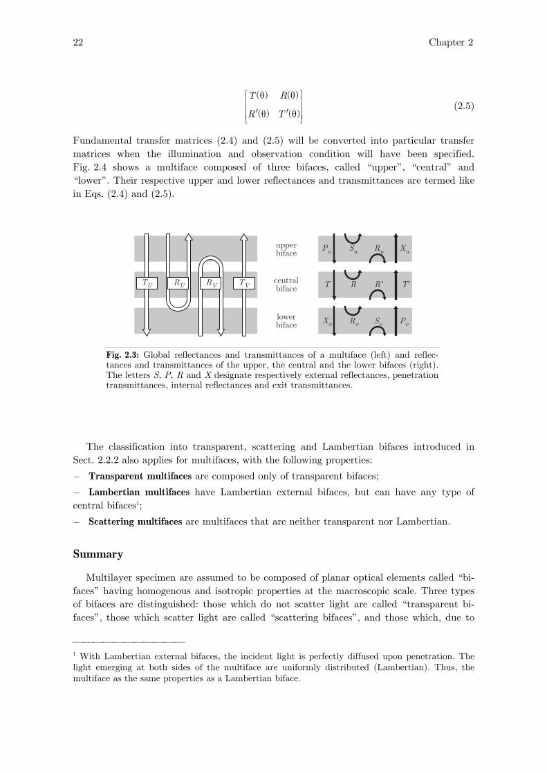
Fundamental transfer matrices (2.4) and (2.5) will be converted into particular transfer matrices when the illumination and observation condition will have been specified. Fig. 2.4 shows a multiface composed of three bifaces, called “upper”, “central” and “lower”. Their respective upper and lower reflectances and transmittances are termed like in Eqs. (2.4) and (2.5).
upperbiface
centralbiface
lowerbiface
RU TVTU RV T R R'
Pu Su
T'
Xu
PvSvXv Rv
Ru
Fig. 2.3: Global reflectances and transmittances of a multiface (left) and reflec-tances and transmittances of the upper, the central and the lower bifaces (right). The letters S, P, R and X designate respectively external reflectances, penetration transmittances, internal reflectances and exit transmittances.
The classification into transparent, scattering and Lambertian bifaces introduced in Sect. 2.2.2 also applies for multifaces, with the following properties:
− Transparent multifaces are composed only of transparent bifaces;
− Lambertian multifaces have Lambertian external bifaces, but can have any type of central bifaces1;
− Scattering multifaces are multifaces that are neither transparent nor Lambertian.
Summary
Multilayer specimen are assumed to be composed of planar optical elements called “bi-faces” having homogenous and isotropic properties at the macroscopic scale. Three types of bifaces are distinguished: those which do not scatter light are called “transparent bi-faces”, those which scatter light are called “scattering bifaces”, and those which, due to
⎯⎯⎯⎯⎯⎯⎯⎯⎯⎯⎯ 1 With Lambertian external bifaces, the incident light is perfectly diffused upon penetration. The light emerging at both sides of the multiface are uniformly distributed (Lambertian). Thus, the multiface as the same properties as a Lambertian biface.

Faces, bifaces and multifaces 23
strong scattering, reflect and transmit Lambertian light independently of the geometry of illumination are called “Lambertian bifaces”.
A biface has two “faces” corresponding to its two lightenable sides. Each face is char-acterized by its directional reflectance and transmittance. Thus, the biface is character-ized by a “fundamental transfer matrix” containing the directional reflectances and transmittances of its two faces. Lambertian bifaces are an exception, since their face re-flectance and transmittance are invariant. They are characterized by an “invariant trans-fer matrix”.
When specific geometries of illumination and observation are considered, faces have a particular reflectance and transmittance and bifaces have a “particular transfer matrix”. When the geometry of observation is not specified, it should be considered that the solid angle of observation is the whole hemisphere.
The multifaces result from the superposition of bifaces. The two bifaces in direct con-tact with the surrounding media are called “external”. They are characterized by an “ex-ternal reflectance”, a “penetration transmittance”, an “internal reflectance” and an “exit transmittance”.
The two next chapters are dedicated to the characteristics of transparent bifaces (Chapter 3), of scattering and Lambertian bifaces (Chapter 4), and of multifaces (Chap-ter 5). The specification of the illumination and observation geometries is presented in Chapter 6, where the terminology specific to the external bifaces will be used.


25
Chapter 3.
Optical properties of transparent bifaces
Transparent bifaces reflect and transmit light without scattering. Directional light is split into a pair of reflection and transmission directions, called the regular directions, which are determined by Snell’s laws (Sect. 2.1). When the two surrounding media have different refractive indices, the directions of transmission and of incidence are different. We have three types of transparent bifaces: flat interfaces, characterized by the Fresnel formulae (Sect. 2.2), transparent layers, characterized by Beer’s law (Sect. 2.3), and transparent multifaces, resulting from the superposition of flat inter-faces and transparent layers. Sect. 2.4 presents one example of transparent multiface, composed of a transparent layer bounded by flat interfaces.
3.1 Generalities on transparent bifaces
Bifaces are transparent when they do not scatter light (Sect. 2.3). The images of an object that they reflect and transmit are perfectly clear. Among the transparent bifaces, we find the flat interfaces between two media of different refractive indices, and the trans-parent layers, i.e. the absorbing but nonscattering layers of constant thickness. Stacked transparent layers, composed of an alternation of transparent layers and flat interfaces, are also transparent bifaces since none of their components scatter light. Mirrors are spe-cial cases, composed of only one face having a zero transmittance.
The two faces of transparent bifaces may have a different reflectance and a different transmittance. However, both faces reflect and transmit a directional incident light into a single pair of directions, the regular directions, determined by Snell’s laws. They are com-pletely characterized by their directional reflectance and transmittance, from which one may deduce their diffuse and Lambertian reflectances and transmittances.
3.1.1 Snell’s laws
The principal characteristic of transparent faces consists of the bijective relations exist-ing between the directions of incidence, of reflection and of transmission.
Let us consider an incident flux coming from direction ( ),i iθ φ , also denoted by the differential solid angle idω =sin i i id dθ θ φ . The reflected and transmitted fluxes are also di-rectional, flowing respectively into directions ( ),r rθ φ and ( ),t tθ φ , denoted by the differen-tial solid angles sinr r r rd d dω = θ θ φ and sint t t td d dω = θ θ φ (Fig. 3.1). These directions are related by Snell’s laws, which are generally formulated for flat interfaces, but still remain valid for any transparent biface:
1. The three directions of incidence, of reflection and of transmission belong to a same plane, the plane of incidence, also containing the normal of the face. Therefore, zenithal

26 Chapter 3
angles are such that r t iφ = φ = φ + π .
2. The angles of reflection and of incidence are equal, i.e. .r iθ = θ
3. The angles of transmission and of incidence are related by the “sine formula” involv-ing the refractive indices of the biface’s surrounding media, ni and nt
sin sini i t tn nθ = θ (3.1)
Reflection and transmission directions given by Snell’s laws are called the regular direc-tions. The regular direction of reflection is also called specular direction. When the media surrounding the transparent biface have different refractive indices ( i tn n≠ ), the direc-tion of transmission differs from the direction of incidence and is called direction of re-fraction.
dωi
dωr = dωi
dωt
θr
θt
Transparent biface
θi
φi
φr = φt
ni
nt
Fig. 3.1: Directional incident flux illuminating a transparent face surrounded by media of respective refractive indices ni ≠ nt. The incidence, the reflection and the transmission solid angles belong to the plane of incidence. The reflection con-serves the angle and the solid angle of incidence. The refraction modifies the angle and the solid angle of incidence.
Let us find the relationship between dωi, dωr and dωt. According to Snell’s first law, one has i r td d dφ = φ = φ . It follows from Snell’s second law that sin sini i r rd dθ θ = θ θ and therefore that the reflection and incidence solid angles are equal ( r id dω = ω ). For the transmission, by differentiating Eq. (3.1), one finds that cosi i in dθ θ cost t tn d= θ θ . Let us write the member-by-member product of this relation with Eq. (3.1), and multiply both sides with the azimuthal solid angles i td dφ = φ . One obtains
sin cos sin cosi i i i i i t t t t t tn n d d n n d dθ ⋅ θ θ ⋅ φ = θ ⋅ θ θ ⋅ φ (3.2)
which may be written as
2 2cos cosi i i t t tn d n dθ ω = θ ω (3.3)

Optical properties of transparent bifaces 27
Obviously, when ni = nt, the incident light exits the transparent biface in the same direction as the direction of incidence, with the same solid angle.
3.1.2 Radiance invariance at a transparent face
We are now interested in the transmission of directional flux across a transparent bi-face. We would like to find the relationship1 between the incident radiance Li and the transmitted radiance Lr.
The solid angles associated to these radiances satisfy Eq. (3.3). By multiplying both members of Eq. (3.3) by an elemental area ds, one obtains the relation
2 2cos cosi i i t t tn ds d n ds dθ ω = θ ω (3.4)
which generalizes the principle of reciprocity of transfer volume expressed by Eq. (1.11). The incident element of flux 2
id Φ is attenuated by a factor ( )iT θ when crossing the bi-face, ( )iT θ being the directional transmittance of the biface. The transmitted flux is
( )2 2it id T dθΦ = Φ . The transmitted radiance Lt is
( )
( )( )
222 2
2cos cos/ cos
ti it iit
it t i ii t i i
nT dd dL T
nds d ds dn n ds d
θ Φ ⎛ ⎞Φ Φ⎟⎜ θ= = = ⎟⎜ ⎟⎜⎝ ⎠θ ω θ ωθ ω (3.5)
The righter fraction in Eq. (3.5) corresponds to the incident radiance Li
( )2
tit i
i
nL T Ln
⎛ ⎞⎟⎜ θ= ⎟⎜ ⎟⎜⎝ ⎠ (3.6)
Eq. (3.6) generalizes the radiance invariance principle expressed by Eq. (1.12), embodying the refraction at the interface [Wol98]. The term ( )2
/t in n , characterizing the effect of the refraction, becomes one as the two media surrounding the transparent biface are of same refractive index.
Remark: We may develop a similar expression as (3.6) for the reflection of radiance. It can be easily shown that
( )r i iL R L= θ (3.7)
with ( )iR θ the directional reflectance of the transparent biface.
3.1.3 Reflectance and transmittance of transparent bifaces
A transparent face is completely characterized by its directional reflectance R(θ) and its directional transmittance T(θ), which may be directly determined by optical laws (e.g. Fresnel formulae for flat interfaces or Beer’s law for transparent layers) or should be ob-tained using a model (e,g., for stacked transparent layers having different refractive indi-ces, by a multiple reflection transmission model).
⎯⎯⎯⎯⎯⎯⎯⎯⎯⎯⎯ 1 This relation has been established by McCluney in [McCL94, p. 112] in the particular case of a flat interface between two media of different refractive indices.

28 Chapter 3
The polarization of the incident light shall be taken into account. We consider natural light, which is modeled as the sum of two independent linearly polarized components: a component polarized in parallel to the incidence plane, and a component polarized per-pendicularly [BW99, p. 47]. We note iE ⊥ and iE the corresponding irradiances and Ei the total irradiance of natural light
i i iE E E⊥= + (3.8)
Since natural light is unpolarized in average, the polarized irradiances are equal
2
ii i
EE E⊥ = = (3.9)
When the irradiance Ei is reflected by a transparent biface, the reflected irradiance Er is composed of a parallel component ( ) r iE R E⊥ ⊥ ⊥= θ and a perpendicular component
( ) r iE R E= θ . The directional reflectance R(θ) for incident natural light is
( ) ( ) ( )12
R R R⊥⎡ ⎤θ = θ + θ⎢ ⎥⎣ ⎦ (3.10)
Likewise, the directional transmittance T(θ) for incident natural light is
( ) ( ) ( )[ ]
12
T T T⊥θ = θ + θ (3.11)
Every transparent face is characterized by a fundamental transfer matrix whose elements are its upper and lower directional reflectances and transmittances for natural light
( ) ( )
( ) ( )
u u
v v
T R
R T
⎡ ⎤θ θ⎢ ⎥⎢ ⎥θ θ⎢ ⎥⎣ ⎦
(3.12)
3.2 Flat interfaces
Two media of different refractive indices have in common a planar border called inter-face. If one of the media is metallic, its refractive index is a complex number, whose real part ν represents the simple index of refraction and whose imaginary part κ represents the attenuation index [BW99, p. 737], also called extinction coefficient. The interface has a relative index of refraction 1 0/n n n= defined as the ratio of the refractive index of the medium of transmission (n1) to the refractive index of the medium of incidence (n0).
3.2.1 Fresnel formulae
The fractions of directional incident flux (or element of irradiance) that are reflected and transmitted by the interface are respectively called reflection coefficient and trans-mission coefficient. They are given by Fresnel formulae. They depend on the relative re-fractive index of the interface and the direction and the polarization of the incident light. The notions presented here are stated in detail in [BW99, pp. 40–53].

Optical properties of transparent bifaces 29
T01(ψ0) R10(ψ1)
T10(ψ1)R01(ψ0)
n0
n1
ψ0ψ0 ψ0
ψ1 ψ1 ψ1
Fig. 3.2: Fresnel reflection and transmission coefficients giving the directional re-flectances and transmittances of both faces of a flat interface between two media of refractive indices n0 and n1.
Let us consider a directional light coming from medium 0 at angle θ0. The corresponding angle of refraction is ( )1 0arcsin sin /nθ = θ [Eq. (3.1)]. When n is complex (metallic reflec-tion), θ1 is a complex angle having therefore only an algebraic meaning. For the perpen-dicular component the reflection coefficient ( )01 0R⊥ θ is
( )( )( )
20 1
01 0 20 1
sin
sinR⊥ θ − θ
θ =θ + θ
(3.13)
For the parallel component, the reflection coefficient is
( )( )( )
20 1
01 0 20 1
tan
tanR
θ − θθ =
θ + θ (3.14)
Fresnel formulae (3.13) and (3.14) can also be presented under an expanded form as func-tions of the angle of incidence θ0, and the relative index of refraction of the interface n i= ν + κ [Gla95]
( )( )( )
2 20
01 0 2 20
cos
cos
a bR
a b⊥ − θ +
θ =+ θ +
(3.15)
and
( ) ( )( )( )
2 20 0
01 0 01 0 2 20 0
cos 1/cos
cos 1/cos
a bR R
a b⊥ + θ − θ +
θ = θ− θ + θ +
(3.16)
with a and b given by
( ) ( )
( ) ( )
22 2 2 2 2 2 2 2 20 0
22 2 2 2 2 2 2 2 20 0
2 sin 4 sin
2 sin 4 sin
a
b
= ν − κ − θ + ν κ + ν − κ − θ
= ν − κ − θ + ν κ − ν − κ − θ (3.17)
When both media have a real refractive index, the relative index of refraction of the inter-face n is also real. The reflection and the transmission are said to be vitreous. The Fresnel formulae become
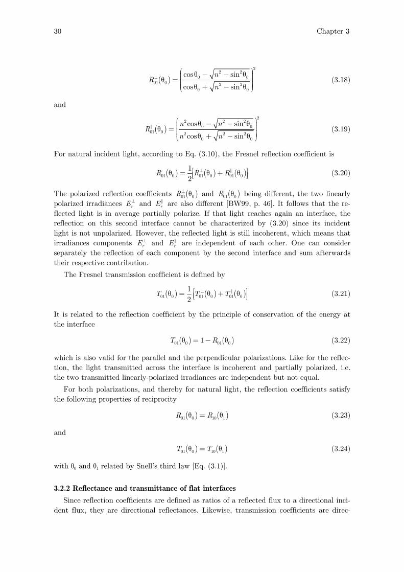
30 Chapter 3
( )
22 2
0 001 0 2 2
0 0
cos sin
cos sin
nR
n⊥
⎛ ⎞θ − − θ ⎟⎜ ⎟⎜θ = ⎟⎜ ⎟⎜ ⎟⎟⎜ θ + − θ⎝ ⎠ (3.18)
and
( )
22 2 2
0 001 0 2 2 2
0 0
cos sin
cos sin
n nR
n n
⎛ ⎞θ − − θ ⎟⎜ ⎟⎜θ = ⎟⎜ ⎟⎜ ⎟⎟⎜ θ + − θ⎝ ⎠ (3.19)
For natural incident light, according to Eq. (3.10), the Fresnel reflection coefficient is
( ) ( ) ( )01 0 01 0 01 0
12
R R R⊥⎡ ⎤θ = θ + θ⎢ ⎥⎣ ⎦ (3.20)
The polarized reflection coefficients ( )01 0R⊥ θ and ( )01 0R θ being different, the two linearly polarized irradiances rE ⊥ and rE are also different [BW99, p. 46]. It follows that the re-flected light is in average partially polarize. If that light reaches again an interface, the reflection on this second interface cannot be characterized by (3.20) since its incident light is not unpolarized. However, the reflected light is still incoherent, which means that irradiances components rE ⊥ and rE are independent of each other. One can consider separately the reflection of each component by the second interface and sum afterwards their respective contribution.
The Fresnel transmission coefficient is defined by
( ) ( ) ( ) 01 0 01 0 01 0
12
T T T⊥⎡ ⎤θ = θ + θ⎢ ⎥⎣ ⎦ (3.21)
It is related to the reflection coefficient by the principle of conservation of the energy at the interface
( ) ( )01 0 01 01T Rθ = − θ (3.22)
which is also valid for the parallel and the perpendicular polarizations. Like for the reflec-tion, the light transmitted across the interface is incoherent and partially polarized, i.e. the two transmitted linearly-polarized irradiances are independent but not equal.
For both polarizations, and thereby for natural light, the reflection coefficients satisfy the following properties of reciprocity
( ) ( )01 0 10 1R Rθ = θ (3.23)
and
( ) ( )01 0 10 1T Tθ = θ (3.24)
with θ0 and θ1 related by Snell’s third law [Eq. (3.1)].
3.2.2 Reflectance and transmittance of flat interfaces
Since reflection coefficients are defined as ratios of a reflected flux to a directional inci-dent flux, they are directional reflectances. Likewise, transmission coefficients are direc-

Optical properties of transparent bifaces 31
tional transmittances. Therefore, flat interfaces between media of refractive indices n0 and n1 have the fundamental transfer matrix
( ) ( )
( ) ( )
01 01
10 10
T R
R T
⎡ ⎤θ θ⎢ ⎥⎢ ⎥θ θ⎢ ⎥⎣ ⎦
(3.25)
In Fig. 3.2, the flat interface is illuminated at angle ψ on its upper face and at angle ψ1 on its lower face. Using the notations introduced in Sect. 2.3 for such an illumination geome-try, the interface has the particular transfer matrix
( ) ( ) ( )
( ) ( )( )
( ) ( )
( ) ( )
0
1
01 01 01 0 01 0
10 10 10 1 10 1
dir
dir
T R T R
R T R T
ψ →
← ψ
⎡ ⎤ ⎡ ⎤θ θ ψ ψ⎢ ⎥ ⎢ ⎥=⎢ ⎥ ⎢ ⎥θ θ ψ ψ⎢ ⎥ ⎢ ⎥⎣ ⎦ ⎣ ⎦ (3.26)
Let us now consider Lambertian illuminations. The Lambertian reflectance and transmit-tance of the upper face are called r01 and t01. Those of the lower face are called r01 and t01. They derive from Fresnel reflection and transmission coefficients, which are directional reflectances and transmittances, according to Eq. (1.29)
( )
2
01 010
sin2r R dπ
θ== θ θ θ∫ , (3.27)
( )
2
01 010
sin2t T dπ
θ== θ θ θ∫ , (3.28)
( )
2
10 100
sin2r R dπ
θ== θ θ θ∫ , (3.29)
and
( )
2
10 100
sin2t T dπ
θ== θ θ θ∫ (3.30)
Properties (3.22), (3.23) and (3.24) of Fresnel formulae permit to establish the relation-ship between r01, t01, r10 and t10. Eq. (3.22) represents the conservation of energy at the interface for directional illumination. Energy is also conserved for Lambertian illumina-tions
01 01 1r t+ = and 10 10 1r t+ = (3.31)
There also exists a relation between t10 and t01. In (3.30), integration is performed accord-ing to the angle in the upper medium (now denoted θ0). Thanks to the bijective relation between θ0 and the angle θ1 beneath the interface, one can perform a change of variable and integrate according to θ1. Relation (3.24) gives T10(θ1) = T01(θ0). The reciprocity of transfer volume (see Sect. 1.1.3), yields
20 0 0sin2n dθ θ 2
1 1 1sin2n d= θ θ . Thus, t10 becomes
( ) ( ) ( )
0 0
2 2210 10 0 0 0 0 1 01 0 0 0
0 0sin2 / sin2t T d n n T d
π π
θ = θ == θ θ θ = θ θ θ∫ ∫ (3.32)
where the most right integral corresponds to t01 [Eq. (3.28)]. The Lambertian transmit-tances of the upper and the lower faces of a flat interface are therefore related by

32 Chapter 3
( )210 0 1 01/t n n t= (3.33)
When both its faces receive a Lambertian illumination, using the notation introduced in Sect. 2.3, the flat interface has the particular transfer matrix
( ) ( )
( ) ( )
01 0101 01 01 01
2 210 10 01 0110 10
1
1 / /
L
L
t tT R t r
r t t n t nR T
→
←
⎡ ⎤ ⎡ − ⎤θ θ ⎡ ⎤⎢ ⎥ ⎢ ⎥⎢ ⎥= =⎢ ⎥ ⎢ ⎥⎢ ⎥ −θ θ⎢ ⎥ ⎢ ⎥⎣ ⎦ ⎣ ⎦⎣ ⎦ (3.34)
Judd [Jud42] tabulated the values of directional (0° and 45°) and Lambertian reflectances and transmittances for real relative refractive indices comprised between 1 and 2. For instance, considering an interface of refractive index 1.5, Eq. (3.34) takes the values
01 01
10 10
0.9 0.1
0.6 0.4
t r
r t
⎡ ⎤⎡ ⎤ ⎢ ⎥⎢ ⎥ ⎢ ⎥⎢ ⎥ ⎢ ⎥⎣ ⎦ ⎣ ⎦ (3.35)
3.3 Transparent layers
Transparent layers are layers made of a homogenous absorbing but nonscattering me-dium having flat and parallel boundaries. Light crosses them along a straight line without reflection. They have therefore a null BRDF and a null reflectance. Their two faces have the same directional transmittance T(θ), determined by Beer’s law. They are always con-sidered separately from their bounding interfaces, i.e. they are assumed to have the same refractive index as their surrounding media.
3.3.1 Beer’s law
A directional flux traversing a path of length x within a nonscattering medium of ab-sorption coefficient α is attenuated by a factor Θ given by Beer’s law [Per95]
xe−αΘ = (3.36)
3.3.2 Transmittance of a transparent layer
Directional light crossing a transparent layer perpendicularly to its surface is attenu-ated by a factor t, called normal transmittance of the layer. It is assumed to be independ-ent of the polarization of the incident light. According to Beer’s law, t is a function of the layer’s thickness h and of its absorption coefficient α
ht e−α= (3.37)
When directional light comes at angle θ, the length of its path across the layer is h/cosθ (Fig. 3.3). It is attenuated by a factor T(θ) that may be expressed as a function of the normal transmittance t
( ) /cos 1/coshT e t−α θ θθ = = (3.38)
T(θ) is the directional transmittance of the transparent layer. The exponent 1/cosθ is called the relative path length of the oblique light.

Optical properties of transparent bifaces 33
θh
h/cosθ
Fig. 3.3: Path length traversed by a light ray crossing at angle θ a transparent layer of thickness h.
The fundamental transfer matrix of a transparent layer is
1/cos
1/cos
0
0
t
t
θ
θ
⎡ ⎤⎢ ⎥⎢ ⎥⎢ ⎥⎣ ⎦
(3.39)
Its Lambertian transmittance T is derived from its directional transmittance according to Eq. (1.29)
( )
/2 /21/cos
0 0sin2 sin2T T d t d
π πθ
θ= θ== θ θ θ = θ θ∫ ∫ (3.40)
3.3.3 Superposed transparent layers
Let us consider k superposed transparent layers having the same refractive index and having respectively the normal transmittances t1, t2, …, tk. They form again a transparent layer, whose normal transmittance t is the product of the normal transmittances ti (i = 1, 2, …, k). The directional transmittance of the multiface is also the product of the respective normal transmittances of the layers
( ) ( ) ( ) ( ) ( )
1/cos1/cos 1/cos 1/cos 1/cos1 2 1 2 1 2... ... ...k k kT t t t t t t t T T Tθθ θ θ θθ = = = = θ θ θ (3.41)
The Lambertian transmittance T of the multiface is expressed as in Eq. (3.40) with the directional transmittance T(θ) given by Eq. (3.41). T cannot be obtained by the product of the respective Lambertian transmittances of the transparent layers. This is simply shown by the inequality
( ) ( ) ( ) ( ) ( ) ( )= θ θ θ θ θ ≠ θ θ θ θ θ θ θ θ θ∫ ∫ ∫ ∫1 2 1 2... sin2 sin2 sin2 ... sin2k kT T T T d T d T d T d (3.42)
Such an inequality is encountered for every transparent multiface: its Lambertian reflec-tance (idem for the transmittance) shall be calculated from its directional reflectance but not from the Lambertian reflectances of its faces. We call this the “principle of direction-ality of multifaces”.
3.4 Transparent multifaces
We just saw a special case of transparent multiface, composed only of transparent lay-ers. Let us now consider superpositions of transparent layers and flat interfaces. When they contain two or more interfaces, light is subject to multiple reflections and transmis-

34 Chapter 3
sions. The reflected and transmitted lights, which are directional if the incident light is directional, are composed of a multitude of components, each one having been multiply reflected and transmitted a certain number of times. We shall first calculate the direc-tional reflectance of the multiface for linearly polarized light, i.e. the parallel component and the perpendicular component. Then the contributions of these components are aver-aged according to Eqs. (3.11).
By way of example, we consider a transparent layer surrounded by two different media of distinct refractive indices. The transparent layer together with its two flat interfaces forms a transparent multiface called “interfaced layer”. The refractive indices of the up-per medium, the layer and the lower medium are denoted respectively n0, n1 and n2. In order to avoid interference phenomena, the transparent layer, having a normal transmit-tance t, has a thickness h significantly larger than the wavelengths of light.
We call ( )012 0R⊥ θ , ( )012 0R θ and ( )012 0R θ the directional reflectances of the interfaced layer defined respectively for a ⊥-polarized, a ||-polarized and an unpolarized incident light coming from medium 0 with an angle θ0. The corresponding directional transmit-tances are called respectively ( )012 0T ⊥ θ , ( )012 0T θ and ( )012 0T θ .
3.4.1 Multiple reflection-transmission of polarized directional light
Directional incident irradiance iE ⊥ , of perpendicular polarization, comes with an angle θ0 from the upper medium (refractive index n0). Once having penetrated the layer, it re-mains directional but is subject to multiple reflections between the interfaces, illustrated by Fig. 3.4. At each interaction with an interface, it is split into a reflected component and a transmitted component. The transmitted components exit definitively the inter-faced layer and contribute to the total reflected irradiance or the total transmitted irradi-ance. The reflected components are alternately reflected by the two interfaces. Our goal is to express the total reflected and transmitted irradiances, called rE ⊥ and tE ⊥ .
Er0 Er1 Er2
Et1 Et2 Et3
Er3Ei
n0
n1
n2
i01
i12
θ0θ0
θ1θ1 θ1
θ2
Fig. 3.4: Multiple reflection-transmission of light within a transparent layer inter-faced by two flat interfaces.

Optical properties of transparent bifaces 35
During the multiple reflection-transmission process, light remains in the plane of incidence and therefore follows a constant azimuthal direction (Snell’s first law, Sect. 3.1.1). How-ever, according to the medium in which it propagates, it follows different zenithal angles, noted θ0 in the upper medium, θ1 in the transparent layer and θ2 in the lower medium. According to Snell’s third law, angles θ1 and θ2 are related to θ0 by
0 0 1 1 2 2sin sin sinn n nθ = θ = θ (3.43)
Let us express the irradiance components emerging successively in the upper and the lower surrounding media. A fraction ( )01 0R⊥ θ of the incident irradiance iE ⊥ is reflected by the interface i01 and follows the specular direction. This reflected component forms an irradiance ( )0 01 0 r iE R E⊥ ⊥ ⊥= θ , which is a first contribution to the total reflected irradiance
rE ⊥ .
A fraction ( )01 0T ⊥ θ of iE ⊥ is refracted into the layer. Along its path of relative length 11/cosθ across the layer, the transmitted light is attenuated by a factor 11/cost θ due to
absorption (Beer’s law). Once having reached the interface i12, the irradiance ( )
11/cos
01 0 iT t E⊥ θ ⊥θ is transmitted into the lower medium (fraction ( )12 1T ⊥ θ ) and reflected back into the layer (fraction ( )12 1R⊥ θ ). The irradiance transmitted into the lower medium, called 0tE ⊥ , is the first contribution to the total transmitted irradiance tE ⊥ .
( ) ( )
11/cos
0 01 0 12 1t iE T T t E⊥ ⊥ ⊥ θ ⊥= θ θ (3.44)
The irradiance reflected back into the layer, equal to ( ) ( ) 11/cos01 0 12 1 iT R t E⊥ ⊥ θ ⊥θ θ , crosses again
the layer (attenuation factor 11/cost θ due to absorption) and is either internally reflected by the interface i01 (Fresnel reflection factor ( )10 1R⊥ θ ), or transmitted (Fresnel transmission factor ( )10 1T ⊥ θ ) into the upper medium. This irradiance transmitted into the upper me-dium, 1rE ⊥ , is the second contribution to the total reflected irradiance rE ⊥
( ) ( ) ( )
12/cos
1 01 0 12 1 10 1 r iE T R T t E⊥ ⊥ ⊥ ⊥ θ ⊥= θ θ θ (3.45)
Then, light continues to be alternately reflected by interfaces i01 and i12, with an irradi-ance component exiting the interfaced layer simultaneously to each reflection. By express-ing the successive irradiances rkE ⊥ exiting in the upper medium and summing them, we obtain the total reflected irradiance, from which we deduce the reflectance of the inter-faced layer for the perpendicularly-polarized component. The same is done for the trans-mittance. The kth irradiance exiting into the upper medium, called rkE ⊥ , crosses 2k times the layer and is internally reflected k times by the interface i12 and k−1 times by the in-terface i10. The generic expression for rkE ⊥ is therefore
( ) ( ) ( ) ( ) ( ) ( ) 1
1 2 /cos01 0 10 1 12 1 1 10 1 for 1, 2, 3...
k k krk iE T R R t T E k
−⊥ ⊥ ⊥ ⊥ θ ⊥ ⊥⎡ ⎤ ⎡ ⎤= θ θ θ θ θ =⎣ ⎦ ⎣ ⎦ (3.46)
The sum of the reflected irradiances rkE ⊥ ( 0, 1, 2...k = ) yields the total reflected irradi-ance rE ⊥
( )( ) ( )
( )( ) ( )
101 0 10 1 2/cos
01 0 10 1 12 1110 1
k
rk i ik
T TE R E E R R t
R
⊥ ⊥ ∞⊥ ⊥ ⊥ ⊥ ⊥ ⊥ θ
⊥=
θ θ ⎡ ⎤= θ + θ θ⎢ ⎥⎣ ⎦θ ∑ (3.47)
The infinite sum is a geometrical series. Since θ0 and θ1 are related by Snell’s law, we have

36 Chapter 3
( ) ( )10 1 01 0T T⊥ ⊥θ = θ . Eq. (3.47) can be simplified as
( )( ) ( )
( ) ( )
1
1
2 2/cos10 1 12 1
01 0 2/cos10 1 12 1
1r i i
T R tE R E E
R R t
⊥ ⊥ θ⊥ ⊥ ⊥ ⊥
⊥ ⊥ θ
⎡ ⎤θ θ⎣ ⎦= θ +− θ θ
(3.48)
Similarly, the kth irradiance exiting into the lower medium, called tkE ⊥ , crosses 2 1k + times the layer. It is internally reflected k times by the interface i12 and k times by the interface i10. The generic expression for tkE ⊥ is therefore
( ) ( ) ( ) ( )
1
2 1cos
01 0 10 1 12 1 12 1 (for 0, 1, 2, 3...)k
k k
tk iE T R R t T E k+
⊥ ⊥ ⊥ ⊥ θ ⊥ ⊥⎡ ⎤ ⎡ ⎤= θ θ θ θ =⎣ ⎦ ⎣ ⎦ (3.49)
The sum of the transmitted irradiances tkE ⊥ yielding a geometric series, gives tE ⊥
( ) ( ) ( ) ( )( ) ( )
( ) ( )
1
1 1
1
1/cos01 0 12 11/cos 2/cos
01 0 12 1 10 1 12 1 2/cos0 10 1 12 1
1
k
t i ik
T T tE T T t E R R t E
R R t
⊥ ⊥ θ∞⊥ ⊥ ⊥ θ ⊥ ⊥ ⊥ θ ⊥
⊥ ⊥ θ=
θ θ⎡ ⎤= θ θ θ θ =⎢ ⎥⎣ ⎦ − θ θ∑ (3.50)
3.4.2 Directional reflectance and transmittance for polarized and natural light
The directional reflectance ( )012 0R⊥ θ and transmittance ( )012 0T ⊥ θ for perpendicularly-polarized incident light are given respectively by the ratio /r iE E⊥ ⊥ deduced from Eq. (3.48)
( ) ( )( ) ( )
( ) ( )
1
1
2 2/cos10 1 12 1
012 0 01 0 2/cos10 1 12 1
1
T R tR R
R R t
⊥ ⊥ θ⊥ ⊥
⊥ ⊥ θ
⎡ ⎤θ θ⎣ ⎦θ = θ +− θ θ
(3.51)
and by the ratio /t iE E⊥ ⊥ deduced from Eq. (3.50)
( )( ) ( )
( ) ( )
1
1
1/cos01 0 12 1
012 0 2/cos10 1 12 11
T T tT
R R t
⊥ ⊥ θ⊥
⊥ ⊥ θ
θ θθ =
− θ θ (3.52)
Since the parallel and the perpendicular polarization components follow the same path within the interfaced layer, directional reflectance ( )012 0R θ and transmittance ( )012 0T θ are expressed as ( )012 0R⊥ θ and ( )012 0T ⊥ θ with the adequate Fresnel coefficients
( ) ( )( ) ( )
( ) ( )
1
1
2 2/cos10 1 12 1
012 0 01 0 2/cos10 1 12 1
1
T R tR R
R R t
θ
θ
⎡ ⎤θ θ⎣ ⎦θ = θ +− θ θ
(3.53)
and
( )( ) ( )
( ) ( )
1
1
1/cos01 0 12 1
012 0 2/cos10 1 12 11
T T tT
R R t
θ
θ
θ θθ =
− θ θ (3.54)
For natural incident light, the expressions obtained for the perpendicular and the parallel polarization components are averaged
( ) ( ) ( ) 012 0 012 0 012 0
12
R R R⊥⎡ ⎤θ = θ + θ⎢ ⎥⎣ ⎦ and ( ) ( ) ( ) 012 0 012 0 012 0
12
T T T⊥⎡ ⎤θ = θ + θ⎢ ⎥⎣ ⎦ (3.55)

Optical properties of transparent bifaces 37
Let us now consider that the directional light comes from the lower medium with an incidence angle θ2. The description of the multiple reflections occurring within the bonded layer is the same as when light comes from the upper medium. We obtain the same re-flectance and transmittance expressions as above with exchanged subscripts 0 and 2. The reflectance ( )210 2R θ and the transmittance ( )210 2T θ of the interfaced layer are
( ) ( ) ( ) 210 2 210 2 210 2
12
R R R⊥⎡ ⎤θ = θ + θ⎢ ⎥⎣ ⎦ and ( ) ( ) ( ) 210 2 210 2 210 2
12
T T T⊥⎡ ⎤θ = θ + θ⎢ ⎥⎣ ⎦ (3.56)
with
( ) ( )( ) ( )
( ) ( )
1
1
2* * 1/cos12 1 10 1* *
210 2 21 2 * * 2/cos12 1 10 1
1
T R tR R
R R t
θ
θ
⎡ ⎤θ θ⎢ ⎥⎣ ⎦θ = θ +− θ θ
and ( )( ) ( )
( ) ( )
1
1
1/cos21 2 10 1
210 2 2/cos12 1 10 1
1
T T tT
R R t
∗ ∗ θ∗
∗ ∗ θ
θ θθ =
− θ θ(3.57)
where the symbol * represents either ⊥ or .
Remark: Let us consider the reciprocity of the directional transmittance of the interfaced layer. According to relation (3.43), we can take Fresnel coefficients ( )10 1T ∗ θ and ( )21 2T ∗ θ in place of ( )01 0T ∗ θ and ( )12 1T ∗ θ . Thus, the expression (3.57) for ( )012 0T ∗ θ and the expression for ( )012 0T ∗ θ become identical, for the two polarization components and thereby for natural light
( ) ( )210 2 012 0T Tθ = θ (3.58)
Summary
The directional reflectance and transmittance are fundamental functions for the trans-parent bifaces since they permit to derive the other types of reflectance and transmittance (diffuse and Lambertian). In the case of a flat interface, they are given by Fresnel formu-lae, and in the case of the transparent layers they are derived from Beer’s law. In the case of transparent multifaces, resulting from the superposition of transparent layers and flat interfaces, the directional reflectance and transmittance depend on the polarization of the incident light, due to the Fresnel formulae. Their diffuse and Lambertian reflectances and transmittances must be derived from the directional reflectance and transmittance (“prin-ciple of directionality”).
As an example of transparent multiface with two flat interfaces, we have developed the directional reflectance and transmittance of transparent layers surrounded by media of different refractive indices. The same reasoning line could be followed for transparent multifaces comprising more than two interfaces. One would consider a directional polar-ized incident light, express the contribution of the irradiance components exiting into the upper and the lower surrounding media, and average them to obtain the total reflected and transmitted irradiances [SHH06].
For the sake of simplicity, we propose in Chapter 5 a new formalism and a mathemati-cal method thanks to which the directional reflectance and transmittance of multifaces can be obtained much more easily.


39
Chapter 4.
Optical properties of scattering and Lambertian bifaces
Scattering and Lambertian bifaces scatter light. Directional light is reflected and transmitted into all directions. Using the formalism introduced in Chapter 2, we char-acterize scattering bifaces by their fundamental transfer matrix, whose elements can be derived from BRDFs and BTDFs, themselves obtainable from an appropriate opti-cal model. We draw up a survey of classical scattering models for two main types of scattering bifaces: rough interfaces (Sect. 4.1) and scattering layers (Sect. 4.2). Strongly scattering layers, which correspond to Lambertian bifaces, are presented separately (Sect. 4.3). They are characterized by an invariant transfer matrix, inde-pendently of the geometry of illumination. We show how their invariant upper and lower reflectances and transmittances can be obtained using the Kubelka-Munk model. We introduce a new way of solving the Kubelka-Munk differential equation system using the Laplace transform. We obtain general solutions, convertible into re-flectance and transmittance expressions as the boundary conditions are specified. When the layer has no border, its reflectance and transmittance are called “intrinsic”. More general expressions are also developed considering the presence of a biface at each of its boundaries.
4.1 Rough interfaces
Rough interfaces are scattering bifaces. They reflect and transmit directional incident light into an enlarged set of directions. Their topography may be represented by a ran-dom function h depending on the coordinates x and y of the horizontal plane (Fig. 4.1). Function h is determined by a probability distribution, generally parameterized by a characteristic vertical length, the root-mean-square (r.m.s.) height σ, and by a character-istic horizontal length, the correlation length τ [Sto95]. Another parameter is also com-monly used: the r.m.s. slope m, corresponding to the ratio σ/τ [TS67].
σ
τx
h(x,y) Local slope Local normal vector
Fig. 4.1: Profile of the elevation function h of a rough interface. The random pat-tern has a r.m.s. height σ and a correlation length τ. The r.m.s. slope m of the in-terface is the ratio σ/τ.

40 Chapter 4
Most models assume that the local slope within rough interfaces follows a Gaussian dis-tribution [BS63, Sto95]. In order to ease the application of optical laws, local slopes are converted into local normal vectors [Ger03, HH05], denoted by the differential solid angle
sinh h h hd d dω = θ θ φ (Fig. 5.2). For an isotropic Gaussian distribution of slopes, the prob-ability distribution function D of the normal vector orientations is
( )( )
2 2tan /2
2 32 cos
h m
hh
eD d
m
− θ
ω =π θ
(3.59)
Function D given by Eq. (3.59) is known as the Beckmann function [Sto95, CT82, NIK91]. It depends only on the polar angle θh due to the assumption of roughness azi-muthal isotropy.
N
θh
θt
θt
θr
θi
θi'
θi'
'
dωi
dωh
dωr
dωt
dωh
Fig 5.2: 2D representation of a rough interface. The directional incident light (di-rection denoted by the differential solid angle dωi) hits a small protion of interface having the normal vector dωh. It is reflected and transmitted into directions dωr and dωt respectively.
4.1.1 Directional and Lambertian reflectances of rough interfaces
In our compositional model, rough interfaces are characterized by their fundamental transfer matrix, whose elements are the upper and lower directional reflectances (resp. Ru and Rv) and transmittances (resp. Tu and Tv)
( ) ( )
( ) ( )
u u
v v
T R
R T
⎡ ⎤θ θ⎢ ⎥⎢ ⎥θ θ⎢ ⎥⎣ ⎦
(3.60)
In a recent work [HH05], we have studied the influence of the surface roughness in the reflectance of printed papers. For this purpose, we have considered a rough paper-air in-terface illuminated on its upper side by directional incident light (incident angle ψ) and on its lower side by Lambertian light, coming from the paper substrate. For such illumi-

Optical properties of scattering and Lambertian bifaces 41
nation geometries, using the notations introduced in Sect. 2.3 [see Eq. (2.2)], the rough interface has the particular transfer matrix
( ) ( ) ( )
( ) ( )
( ) ( )dir
u u u u
i iv vL
T R T R
r tR T
ψ →
←
⎡ ⎤θ θ ⎡ ⎤ψ ψ⎢ ⎥ ⎢ ⎥=⎢ ⎥ ⎢ ⎥θ θ⎢ ⎥ ⎢ ⎥⎣ ⎦⎣ ⎦ (3.61)
where ri is a Lambertian reflectance, expressed according to Eq. (1.29)
( )/2
0sin2i vr R d
π
θ== θ θ θ∫ (3.62)
Parameter ri represents the fraction of Lambertian light issued from the paper that is internally reflected by the rough interface. It is central in color prediction models since it determines how much light is subject to multiple reflections between the paper and the interface (see Sects. 6.3.1 and 7.1.1 or [HH04]). It can be deduced from reflectance meas-urements or computed using a model.
We considered a rough air-print interface having a relative refractive index of 1.53. Its slope was assumed to follow a Gaussian distribution function. By modeling the reflection of light on that interface at the print side, we concluded that ri increases with the r.m.s. slope m but in a very small proportion compared to the reflectance r10 [Eq. (3.27)] of a flat interface (Table 4.1). This explains why the Williams-Clapper model (see Sect. 6.3.2) and the Clapper-Yule model (see Sect. 8.3.2), initially restricted to supports having a flat surface (e.g. coated or calendered paper sheets), are also accurate for mate supports [HECC05].
Table 4.1: Evolution with roughness of the Lambertian reflectance ri of a rough interface, with
n = 1.53 (variation to the reflectance of a flat interface in percent)
r.m.s slope m 0 0.05 0.1 0.2
arctan(m) 0° 2.9° 5.7° 11.3°
ri r10 = 0.614 0.614 (0.1 %) 0.615 (0.2 %) 0.618 (0.6 %)
Directional reflectances and transmittances of rough interfaces can be deduced from their BRDF and their BTDF using Eq. (1.21). BRDFs and BTDFs may be determined experimentally [EM00, EM01, Sto95] or computed thanks to an optical model.
4.1.2 BRDF and BTDF models
Two main approaches enable the study of reflection and transmission by rough inter-faces [NIK91]:
− Physical optics, based directly on the electromagnetic wave theory and Maxwell’s equations [BW99, p. 1]. Models relying on physical optics shall be used when the wave-length of light is large or comparable to the characteristic lengths of the roughness pat-
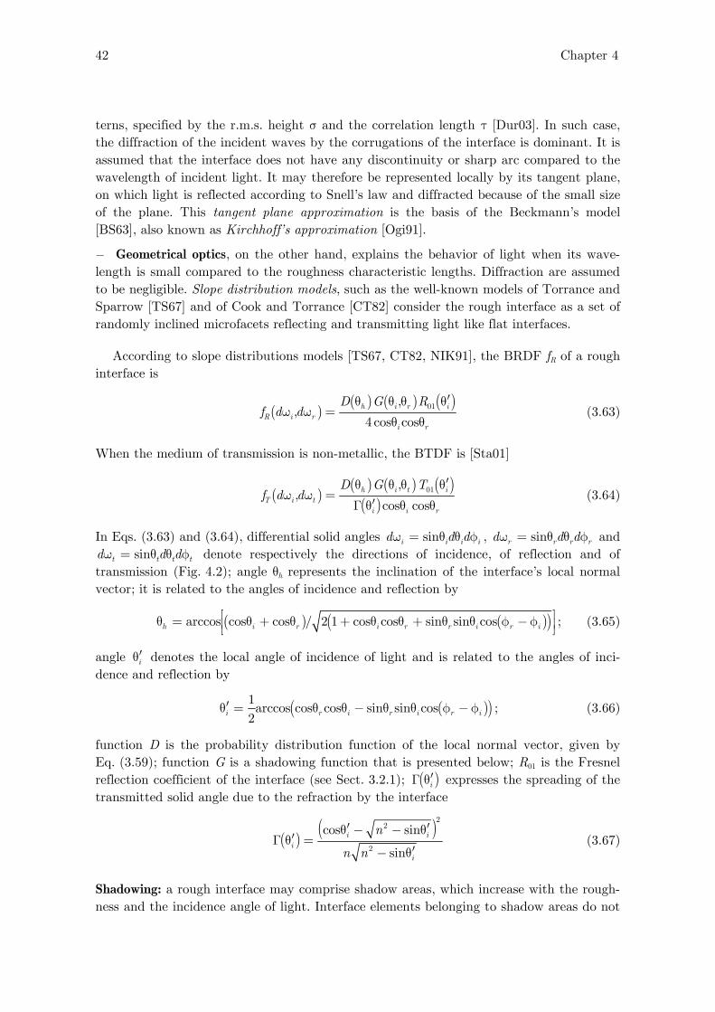
42 Chapter 4
terns, specified by the r.m.s. height σ and the correlation length τ [Dur03]. In such case, the diffraction of the incident waves by the corrugations of the interface is dominant. It is assumed that the interface does not have any discontinuity or sharp arc compared to the wavelength of incident light. It may therefore be represented locally by its tangent plane, on which light is reflected according to Snell’s law and diffracted because of the small size of the plane. This tangent plane approximation is the basis of the Beckmann’s model [BS63], also known as Kirchhoff’s approximation [Ogi91].
− Geometrical optics, on the other hand, explains the behavior of light when its wave-length is small compared to the roughness characteristic lengths. Diffraction are assumed to be negligible. Slope distribution models, such as the well-known models of Torrance and Sparrow [TS67] and of Cook and Torrance [CT82] consider the rough interface as a set of randomly inclined microfacets reflecting and transmitting light like flat interfaces.
According to slope distributions models [TS67, CT82, NIK91], the BRDF fR of a rough interface is
( )( ) ( ) ( )
01,,
4 cos cosh i r i
R i ri r
D G Rf d d
′θ θ θ θω ω =
θ θ (3.63)
When the medium of transmission is non-metallic, the BTDF is [Sta01]
( )( ) ( ) ( )
( )
01,,
cos cosh i t i
T i ti i r
D G Tf d d
′θ θ θ θω ω =
′Γ θ θ θ (3.64)
In Eqs. (3.63) and (3.64), differential solid angles sini i i id d dω = θ θ φ , sinr r r rd d dω = θ θ φ and sint t t td d dω = θ θ φ denote respectively the directions of incidence, of reflection and of
transmission (Fig. 4.2); angle θh represents the inclination of the interface’s local normal vector; it is related to the angles of incidence and reflection by
( ) ( )( ) arccos cos cos / 2 1 cos cos sin sin cosh i r i r r i r i⎡ ⎤θ = θ + θ + θ θ + θ θ φ − φ⎢ ⎥⎣ ⎦
; (3.65)
angle i′θ denotes the local angle of incidence of light and is related to the angles of inci-dence and reflection by
( )( )
1arccos cos cos sin sin cos
2i r i r i r i′θ = θ θ − θ θ φ − φ ; (3.66)
function D is the probability distribution function of the local normal vector, given by Eq. (3.59); function G is a shadowing function that is presented below; R01 is the Fresnel reflection coefficient of the interface (see Sect. 3.2.1); ( )i′Γ θ expresses the spreading of the transmitted solid angle due to the refraction by the interface
( )( )
22
2
cos sin
sin
i ii
i
n
n n
′ ′θ − − θ′Γ θ =
′− θ (3.67)
Shadowing: a rough interface may comprise shadow areas, which increase with the rough-ness and the incidence angle of light. Interface elements belonging to shadow areas do not

Optical properties of scattering and Lambertian bifaces 43
contribute to the reflection nor the transmission. This phenomenon is called shadowing. Likewise, reflected and transmitted light may be partially blocked by neighboring corru-gations. This phenomenon, sometimes called masking [TS67], is equivalent to shadowing but depends on the angle of observation instead of the angle of incidence (Fig. 4.3).
Incident light Reflected light
Rough interface
Shadowing Masking
Fig. 4.3: Some areas (bold line) within the rough interface are not illuminated due to shadowing. Some other areas are not observed due to masking.
The fraction of facets that really contributes to the reflection of light from direction idω to direction rdω is given by function ( ),i rG θ θ , product of two similar functions g, one for shadowing, and the other one for masking
( ) ( ) ( ) ,i r i rG g gθ θ = θ θ (3.68)
Using a statistical model, Smith computed the following shadowing function g [Smi67]
( ) ( )( )
( )
1if cos 0
1,0 if cos 0
imi
i
g
⎧⎪ ′⎪ θ >⎪⎪Λ θ +′θ θ = ⎨⎪⎪ ′θ <⎪⎪⎩
(3.69)
where i′θ is the local angle of incidence given by Eq. (3.66) and where function Λm, pa-rameterized by the surface’s r.m.s. slope m, is defined as
( )
2
2
1 1 2 cotcotexp erfc2 cot 22
m
mmm
⎡ ⎤⎛ ⎞ ⎛ ⎞θθ⎟ ⎟⎜ ⎜⎢ ⎥Λ θ = ⋅ − −⎟ ⎟⎜ ⎜ ⎟⎟ ⎜⎜⎢ ⎥⎝ ⎠⎝ ⎠π θ⎣ ⎦
Note that both functions g in Eq. (3.68) use the same angle i′θ since, according to Snell’s laws, the local angle of incidence is equal to the local angle of reflection (see Fig. 5.2).
Function g is comprised between 0 (facets completely shadowed or masked) and 1 (fac-ets completely illuminated). At small and medium incidence angles, the illuminated frac-tion of the facet’s area is close to 1. The shadowing effect is thus small enough to be ne-glected. However, ignoring the shadowing at high incidence angles may yield an overesti-mation of the reflected and transmitted irradiances, and a subsequent violation of the energy conservation principle. According to Bruce [Bru04] and Caron [CLA02], shadowing should be taken into account when the incidence angle is higher than a limit angle shadθ

44 Chapter 4
depending on the r.m.s. slope m of the rough interface
( )arctan 22shad mπ
θ = − (3.70)
The same considerations apply for masking.
4.2 Scattering layers
The optical properties of a medium are generally characterized by its refractive index. If the latter is constant, a light ray crosses the medium along a straight line without any deviation. However, when light encounters small fluctuations of refractive index within the medium, a portion of the incident light is scattered. In the atmosphere, scattering yields the white color of clouds (Mie scattering [Mie08]), the blue color of the sky [ZB03] and the redness of sunsets (Rayleigh scattering [Ray99]). Scattering also occurs in liquids. Milk, for example, is composed of a suspension of almost transparent fat droplets which scatter light and give to milk its white and opaque aspect. In the case of oceans, scatter-ing is coupled to absorption, which produces the characteristic bluish color. Light is also scattered in solid heterogeneous media, such as painting [Sim02], paper, cotton, human tissues [Pra88], etc.
Different types of scattering are encountered according to the composition, shape, size and concentration of the heterogeneities, often considered as particles immerged into a binder. The polarization and the wavelength of the incident light may have a strong in-fluence on scattering. We present here some commonly used parameters and models rela-tive to scattering, mainly borrowed from the works of Durant [Dur03] and of Simonot [Sim02]. We show in particular the distinction between scattering layers and Lambertian layers, the latter being especially studied in Sect. 4.3.
4.2.1 Scattering parameters
A radiance traversing a path of length x into a scattering and absorbing medium un-dergoes an exponential attenuation T described by the Beer-Lambert law
extK xT e−= (3.71)
where Kext is the extinction coefficient (in m–1). The inverse of the extinction coefficient is the extinction free-mean-path length lext, characterizing the distance along which a radi-ance is attenuated by a factor 1/e
1/ext extl K= (3.72)
The extinction coefficient may be decomposed into a component Ksca relative to scattering and a component Kabs relative to absorption
ext sca absK K K= + (3.73)
Free-mean-path lengths are also defined for scattering lsca and for absorption labs
1/sca scal K= and 1/abs absl K= (3.74)

Optical properties of scattering and Lambertian bifaces 45
The scattering and absorbing medium is said to be homogenous when it has at every point the same coefficients Ksca and Kabs. Note that Beer’s law presented in Sect. 2.3.1 corresponds to the special case where Ksca = 0.
αu
u'
P(u,u')
Fig. 4.4: Phase function of a scattering medium.
As an effect of scattering, the path of light is modified. The change of direction is speci-fied by a phase function, P(u,u′), giving the density of probability for light to be scattered from an initial direction u to a direction u′ (Fig. 4.4). P(u,u′) being a probability, it is always positive and is expected to satisfy the condition of normalization
( )
1, 1
4P d
Σ′ ′ω =
π∫ u u (3.75)
where dω′ is the differential solid angle associated to the outgoing direction u′ and Σ is the entire sphere. When scattering is isotropic, one has P(u,u′) = 1 for every pair of di-rections (u,u′). Otherwise, anisotropic scattering may be characterized by a parameter g defined as the average cosine of the scattering angle
( ) ( )
1, cos ,
4g P d
Σ′ ′ ′= ω
π∫ u u u u (3.76)
The incident light is mainly scattered backwards when g is close to –1 or forwards when g is close to 1. For isotropic scatterings, g = 0. Parameter g is used for defining the trans-port free-mean-path length ltrans, corresponding to the distance from which one may con-sider that light has completely lost the memory of its original direction of incidence
1
scatrans
ll
g=
− (3.77)
The optical thickness τ of a scattering or/and absorbing layer having a thickness h and an extinction coefficient Kext is defined as
extK hτ = (3.78)
When τ 1, a directional incident light is almost completely attenuated. When τ is small, the layer is translucid, i.e. we can distinguish an object located beneath the layer. After a certain number of scattering events, light propagates in an isotropic manner, i.e. it becomes Lambertian.

46 Chapter 4
4.2.2 Types of scattering
The notion of optical thickness defined above allows estimating the number of scatter-ing events that a light ray undergoes across a given layer of the considered medium. In the particular case of a weakly absorbing medium (Kabs Ksca), the optical thickness de-scribes the strength of scattering. We may distinguish four scattering modes, according to the value of the optical thickness of the layer:
− ballistic scattering: τ 1 (h lsca), in which light is almost not scattered,
− single scattering: τ ≈ 1 (h ≈ lsca) in which light is scattered once in the medium (Rayleigh scattering [Ray99], Mie scattering [Mie08]),
− multiple scattering: τ > 1 (h > lsca), in which light is scattered various times [Kor94],
− diffusion: τ 1 (h lsca) where scattering events occur so many times that the re-sulting scattering is isotropic. According to Eq. (3.77), since parameter g defined by Eq. (3.76) is equal to 0, the transport length is given by the scattering length. The inci-dent light has therefore completely lost the memory of its incident direction.
For low concentrations of particles, it is assumed that they do not interact one with each other. Scattering is said to be independent. Describing the scattering by one particle is sufficient to determine the scattering by the whole medium. For high concentrations of particles, scattering becomes dependent. In the case of independence, geometrical optics may be used when the size of the particles are large compared to the wavelength of the incident light. However, when the particles are small compared to the wavelength, light is diffracted. In this case, scattering may be modeled by the Rayleigh scattering theory [Ray71, Ray99, Des91]. The Mie scattering theory describes the diffraction of light by spherical particles of complex refractive index in a dielectric medium (real refractive in-dex) [Mie08]. Note that, excepted for exceptional phenomena such as the Raman effect, scattering does not modify the wavelength of the incident light.
Coming back to the classification of bifaces introduced in Sect. 2.3, we will consider that a layer is transparent when h lsca, Lambertian when h lsca. Otherwise, the layer is considered to be a scattering biface.
4.2.3 The radiative transfer equation
In many applications, a simple phenomenological approach, based on the notion of directed light ray and conservation of energy, provides a realistic description of the scat-tering phenomenon. Considering a sufficiently large portion of the heterogeneous medium, the scattering process is described by a simple equation: the radiative transfer equation [Cha60]. A priori, it is valid only when the scattering free-mean-path length lsca is large compared to the wavelength of the incident light and to the dimension of the heterogenei-ties responsible of the scattering, but specific studies have shown that its domain of valid-ity can be enlarged to other cases [Dur03, Car03].
The radiative transfer equation expresses the conservation of the radiant flux in a given element of volume and a given direction. This energy balance shall be performed everywhere in the medium and in every direction. Let us consider a small cylinder of sec-tion dS and of length dl oriented according to the incident direction u. Radiance L(u) decreases along this direction due to absorption and scattering

Optical properties of scattering and Lambertian bifaces 47
( )
( ) ( )abs sca
dLK K L
dl= − +
uu (3.79)
At the same time, the cylinder receives radiances L(u′) from all directions u′ and scatters them partially towards direction u, which increases radiance L(u). The portion of radi-ance L(u′) that contributes to radiance L(u) is ( ) ( ),scaK P L d
πω′ ′ ′u u u
4, where ( ),P ′u u is the
phase function of the considered cylindrical element of volume. By summing up the con-tributions of all directions u′ and adding the resulting global contribution to Eq. (3.79), one obtains the radiative transfer equation
( ) ( ) ( ) ( ) ( )
Σ′ ′ ′= − + + ω
π ∫u
u u u u,4
scaabs sca
KdLK K L P L d
dl (3.80)
This equation has no general solution. An exact or approximated solution must be searched for every particular scattering medium. Various solutions have been developed. Let us mention the three principal ones [Sim02]:
− The N-fluxes method, which allows converting the integrodifferential equation (3.80) into a differential equation system thanks to an angular discretization. Solutions are ob-tained for azimuthally isotropic media, the discretization being performed only according to the zenithal angle [MR71]; the simplest particular case is the two-flux Kubelka-Munk model [KM31, Kub48]. Four-flux models have also been developed [MLG84, MG86].
− The discrete ordinate method [SCWJ88], which is an exact but computationally expan-sive method. The assumption of azimuthal isotropy is not necessary. Discretization ac-cording to the azimuthal angle is avoided thanks to a Fourier series development for the scattered fluxes and a spherical harmonic decomposition of the phase function.
− The auxiliary function method [EE02], which avoids angular discretization. An auxil-iary function is introduced into the radiative transfer equation and decomposed into spherical harmonics. The radiative transfer equation is thus converted into an integral equation system, which can be solved numerically.
4.3 Lambertian layers
The free-mean-path length lsca of a strongly scattering layer is very small compared to the layer thickness (Sect. 4.2.2). Incident light looses the memory of its initial angular distribution as soon as it penetrates the layer. We can therefore assume that any illumi-nation geometry leads to a same reflectance and a same transmittance, called intrinsic. Since light is scattered a large number of times within the layer, it is Lambertian at every point of the layer, especially at the layer’s bounding planes. We can also assume that light exiting the layer is unpolarized. Strongly scattering layers satisfy the conditions for being a Lambertian biface (Sect. 2.2) and are thus said to be Lambertian layers.
The reflection and transmission by Lambertian layers can be modeled by the Kubelka-Munk two flux model [KM31, Kub48, Kub54], with a satisfying accuracy if the layer is weakly absorbing [Kli71, VN97]. An intent of alternative model relying on Markov chains has been proposed for paper by Simon and Trachsler [ST03]. In the present section, we will present only the Kubelka-Munk model, and propose a new method for solving its famous differential equation system.

48 Chapter 4
4.3.1 Kubelka-Munk two-flux model
The scattering proposed by Kubelka and Munk [KM31] was initially introduced for predicting the reflectance of paints, but it has been also used in a wide range of domains where uniform and infinitely large layers of a scattering medium are encountered. It cor-responds to a special case of the radiative transfer theory where the phase function is re-duced to a pair of opposite directions or, more precisely, of opposite sets of directions covering respectively the upper and the lower hemispheres [Kub54]. Thus, it is said to be a “two-fluxes scattering model”. The model can be equivalently expressed in terms of irradiances instead of fluxes, which corresponds to considering the fluxes relatively to a unit area.
4.3.2 Differential equation system
The interest of the Kubelka-Munk model lies in the simple differential equation system expressing the scattering and absorption phenomena within the layer. The differential equations involve the upward and the downward oriented irradiances, functions of the depth in the layer. Another interest of this model is the fact that the solutions of the dif-ferential equation system have an analytical expression.
The layer, having a thickness h, is made of a homogenous absorbing and scattering medium having an absorption coefficient K and a scattering coefficient S, both ones being functions of the wavelength. In the layer, a Lambertian irradiance ir propagates upwards and a Lambertian irradiance it propagates downwards. Both ir and it are functions of the depth x at which they are located in the layer. Depth 0 corresponds to the layer’s bound-ary that receives the incident irradiance I0. Depth h corresponds to its other boundary (Fig. 4.5).
it(h)
I0
ir(x)
ir(0)
it(0)
ir(x+dx)
it(x+dx)
it(x)dxx
h
0
Fig. 4.5: Upward and downward irradiances crossing a sublayer of thickness dx at a depth x in the scattering layer.
Let us consider at a given depth x a sublayer of infinitesimal thickness dx. The sublayer receives the downward irradiance it (x) on the one side and the upward irradiance ir(x+dx) on the other side. In the sublayer, a fraction S dx of both irradiances ir(x) and it(x) is backscattered, leading to a mutual exchange of irradiance. A fraction K dx is absorbed.

Optical properties of scattering and Lambertian bifaces 49
While crossing the sublayer, the upward irradiance ( )ri x dx+ loses both the absorbed irradiance K ir(x)dx and the backscattered irradiance S ir(x)dx. It gains the backscattered irradiance S it(x)dx. The irradiance it(x) leaving the sublayer is therefore
( ) ( ) ( ) ( ) ( ) r r r ti x i x dx K S i x dx Si x dx= + − + + (3.81)
The downward irradiance it(x) loses the absorbed irradiance K it(x)dx and the backscat-tered irradiance S it(x)dx. It gains the backscattered irradiance S ir(x)dx. The irradiance
( )ti x dx+ leaving the sublayer is
( ) ( ) ( ) ( ) ( ) t t t ri x dx i x K S i x dx Si x dx+ = − + + (3.82)
According to the definition of the derivative, when 0dx →
( ) ( )i x dx i xd
idx dx
+ −= (3.83)
By rearranging Eqs. (3.81) and (3.82), we obtain the Kubelka-Munk differential equation system
( ) ( ) ( ) ( )
( ) ( ) ( ) ( )
r r t
t r t
di x K S i x Si x
dxd
i x Si x K S i xdx
⎧⎪⎪ = + −⎪⎪⎪⎨⎪⎪ = − +⎪⎪⎪⎩
(3.84)
4.3.3 Solutions for the differential equation system
There exists a very simple method for solving the differential equation system (3.84), that we have not found anywhere in the literature. Thanks to the Laplace transform [HS98], we can convert the differential equation system into a linear equation system much more easy to solved.
The Laplace transform associates to a causal function f (x) the function F(p) such that
( ) ( )
0
ptF p f t e dt∞
−= ∫ (3.85)
It is linear, i.e. it transforms ( ) ( ) af x bg x+ into ( ) ( ) aF p bG p+ . The derivative of a func-tion f is transformed into pF(p) – f (0), where the constant f (0) is the value of f at x = 0. Calling Ir(p) and It(p) the respective transforms of ir(x) and it(x), the differential equation system (3.84) is transformed into the following linear equation system, depending on the two unknown functions Ir(p) and It(p)
( ) ( ) ( ) ( ) ( )
( ) ( ) ( ) ( ) ( )
0
0
r r r t
t t r t
pI p i K S I p SI p
pI p i SI p K S I p
⎧ − = + −⎪⎪⎪⎨⎪ − = − +⎪⎪⎩ (3.86)
This system has the two following solutions
( )( )( ) ( )
2 2 2
0 0r tr
i p aS SiI p
p b S
+ −=
− (3.87)

50 Chapter 4
and
( )( )( ) ( )
2 2 2
0 0t rt
i p aS SiI p
p b S
− +=
− (3.88)
with
( )/a K S S= + and 2 1b a= − (3.89)
Since ( )2 2 2/p p b S− and ( )2 2 2/bS p b S− are the respective Laplace transforms of ( ) cosh bSx and ( ) sinh bSx , one concludes1 that Ir(p) is the Laplace transform of
( ) ( ) ( ) ( ) ( )( ) ( )
10 cosh 0 0 sinhr r r ti x i bSx ai i bSx
b= + − (3.90)
and It(p) is the Laplace transform of
( ) ( ) ( ) ( ) ( )( ) ( )
10 cosh 0 0 sinht t r ti x i bSx i ai bSx
b= + − (3.91)
Expressions (3.90) and (3.91) are the general solutions of the Kubelka-Munk differential equation system [HH06].
4.3.4 Intrinsic reflectance and transmittance of a Lambertian layer
Let us now derive from general solutions (3.90) and (3.91) the intrinsic reflectance and transmittance of a scattering layer considered without interface nor any type of biface at its boundaries. An incident irradiance I0 illuminates the upper side of the scattering layer. The intrinsic reflectance of the scattering layer is the fraction of the incident irradiance I0 that exits the layer at the upper side, i.e. the ratio ir(0)/I0. The intrinsic transmittance is the fraction of the incident irradiance I0 exiting at the lower side, i.e. the ratio it(h)/I0. Let us therefore express ir(0) and it(h).
At x = 0, the downward irradiance it (0) is the incident irradiance
it(0) = I0 (3.92)
At x = h, the upward irradiance ir (h) is zero, since the scattering layer is not illuminated from below
ir(h) = 0 (3.93)
By setting x = h and inserting relations (3.92) and (3.93) into Eq. (3.90), one obtains
( )( )
( ) ( )
0
sinh0
cosh sinhr
bShi I
b bSh a bSh=
+ (3.94)
⎯⎯⎯⎯⎯⎯⎯⎯⎯⎯⎯ 1 When a function has a Laplace transform, this latter is unique. The converse is also true. The Laplace transform is bijective from the set of functions admitting a Laplace transform to the set of Laplace transforms.

Optical properties of scattering and Lambertian bifaces 51
Likewise, one takes x = h and replaces, in Eq. (3.91), it(0) and ir(0) by their respective expressions (3.92) and (3.94). One derives from Eq. (3.89) the relation 2 2 1b a= − . Fi-nally, using the classical relation of hyperbolic trigonometry ( ) ( )2 2cosh sinh 1bSh bSh− = , one obtains
( )( ) ( )
0 cosh sinht
bi h I
b bSh a bSh=
+ (3.95)
The ratio ir(0)/I0 gives the intrinsic reflectance ρ of the scattering layer
( ) ( )
( ) ( )
0
sinh0cosh sinh
r bShiI b bSh a bSh
ρ = =+
(3.96)
and the ratio ir(h)/I0 gives its intrinsic transmittance τ
( )
( ) ( ) 0 cosh sinhti h bI b bSh a bSh
τ = =+
(3.97)
As expected, these expressions of intrinsic reflectance and transmittance are identical to those derived by classical solving methods [Kub48].
4.3.5 Lambertian layer bordered by bifaces
Let us now consider that the layer is bounded at x = 0 by a biface whose upper face has a reflectance su and a transmittance pu and whose lower face has a reflectance ru and a transmittance xu. At x = h, the Lambertian layer is bordered by another biface having a reflectance rv and a transmittance xv (Fig. 4.6).
it(h)
I0 Ir
It
ir(x)
ir(0)
ru
supu xu
xv
it(0)
it(x)x
h
0
ir(h)
rv
Lambertian layer
Lower biface
Upper biface
Fig. 4.6: Reflections and transmissions occurring at the boundaries of the Lamber-tian layer.

52 Chapter 4
This biface receives on its upper face an irradiance I0 coming from the light source. A fraction su of I0 is directly reflected and a fraction pu crosses the biface. On its lower face, it receives the upward irradiance ir(0) from the Lambertian layer. A fraction ru is inter-nally reflected and a fraction xu emerges across the biface. Hence, at x = 0, the downward irradiance it(0) is
( ) ( )00 0t u u ri p I r i= + (3.98)
At x = h, the lower biface receives the downward irradiance it(h) and reflects it in a pro-portion rv. There is no light coming from below. Hence, the upward irradiance ir(h) is
( ) ( )r v ti h r i h= (3.99)
Let us insert the boundary equation (3.98) into the general solution (3.90) of ir(x) for x = h, and use the boundary equation (3.99)
( ) ( ) ( ) ( ) ( )[ ] ( )
0
1 10 cosh 0 0 sinht r r u u r
v v
i h i bSh ai p I r i bShr br
⎡ ⎤= + − +⎣ ⎦ (3.100)
We also insert the boundary equation (3.98) into the solution (3.91) of it(x) for x = h
( ) ( )[ ] ( ) ( ) ( )[ ]( ) ( ) 0 0
10 cosh 0 0 sinht u u r r u u ri h p I r i bSh i a p I r i bSh
b= + + − + (3.101)
Eqs. (3.100) and (3.101) form a linear equation system depending on the two unknown variables ir(0) and it(h), i.e. on the two irradiances exiting the print. The solutions of this equation system are
( )( ) ( ) ( )
( ) ( ) ( ) ( )
0
1 sinh cosh0
sinh 1 coshv v
r uu v u v u v
ar bSh b r bShi p I
a r r ar r bSh b r r bSh
− +=
− − + + − (3.102)
and
( )( ) ( ) ( ) ( )
0 sinh 1 cosht uu v u v u v
bi h p I
a r r ar r bSh b r r bSh=
− − + + − (3.103)
A fraction xu of irradiance ir(0) emerges across the upper biface. It forms, conjointly with the irradiance suI0 reflected by the upper biface, a total irradiance Ir
( )0 0r u u rI s I x i= + (3.104)
The ratio Ir/I0 corresponds to the global reflectance Rb of the bordered Lambertian layer
( ) ( ) ( )
( ) ( ) ( ) ( )
1 sinh cosh
sinh 1 coshv v
b u u uu v u v u v
ar bSh br bShR s p x
a r r ar r bSh b r r bSh
− += +
− − + + − (3.105)
Likewise, a fraction xv of irradiance it(h) emerges across the lower biface, forming an emerging irradiance ( )t v tI x i h= . The ratio It/I0 is the global transmittance Tb of the bor-dered Lambertian layer

Optical properties of scattering and Lambertian bifaces 53
( ) ( ) ( ) ( ) sinh 1 coshb u v
u v u v u v
bT p x
a r r ar r bSh b r r bSh=
− − + + − (3.106)
Remark: In the particular case where there is no bordering biface on the upper side, we have su = 0, pu = 1, ru = 0 and xu = 1. By inserting these values into Eqs. (3.105) and (3.106), we obtain the global reflectance and transmittance of the layer bordered only at the lower side
( ) ( ) ( )( ) ( ) ( )
1 sinh cosh
sinh coshv v
kmv
ar bSh br bShR
a r bSh b bSh
− +=
− + (3.107)
and
( ) ( ) ( ) sinh coshkm
v
bT
a r bSh b bSh=
− + (3.108)
These expressions are those presented by Kubelka for the case of a scattering layer bounded at the lower side by a reflecting background of reflectance rv [Kub 31, Kub48].
Let us now consider that, in addition to the background at the lower side, the Lamber-tian layer has an interface at the upper side. We can directly use Eqs. (3.105) and (3.106), where the upper biface represents the interface. However, Eqs. (3.105) and (3.106) are traditionally obtained indirectly via the so-called “Saunderson correction” [Sau42]. Saunderson’s model considers the multiple reflections and transmissions of light between the interface and the Lambertian layer with the background, whose reflectance Rkm and transmittance Tkm are given by (3.107) and (3.108). We will have the opportunity to present this model as a particular case of our compositional model (Sect. 6.3.1).
Summary
We have presented the two types of bifaces by which light is scattered: the scattering bifaces, among which the rough interfaces and scattering layers, and the Lambertian bi-faces. We have presented basic elements of the classical literature that may be used to compute their reflectance and their transmittance.
A homogenous layer where light is intensely scattering is considered as being a Lam-bertian biface. Its reflectance and transmittance, called “intrinsic”, may be modeled using the Kubelka-Munk model. We have presented a solving method for the Kubelka-Munk differential equation system using the Laplace transform. First, general solutions are ob-tained giving the upward and the downward irradiances propagating within the layers as functions of the depth. Then, considering eventual reflections and transmissions taking place at the boundaries of the layer, we can write boundary equations and obtain the global reflectance and transmittance of the Lambertian layer.
More advanced models [Yan04a-c] may also be used when the scattering and absorp-tion coefficients are functions of depth within the layer. Such models are outside the scope of the present study. However, according to our formalism, it is possible to consider non-symmetric layers, with different intrinsic reflectances and transmittances.


55
Chapter 5.
Multiple reflection-transmission of light in multifaces
This chapter is dedicated to the optical properties of multifaces. We first develop a step-by-step description of the transfer of light between the contained faces. The global reflectance and transmittance of the multiface are expressed by infinite sums (Sect. 5.1). Then, we present a special type of multiface, called “regular”, in which light is transferred according to a single reflectance and a single transmittance per face (Sect. 5.2). The infinite sums can be reduced to closed-form expressions. The su-perposition of bifaces is algebraically represented by an operation on their transfer matrices, called “composition”. The composition of two, resp. three bifaces are char-acterized by a “quadriface formula”, resp. a “hexaface formula”. These two composi-tional formulae are developed using Markov chains. They can be further composed it-eratively (Sect. 5.3). Lastly, we complete our new formalism with the notion of “bi-face splitting”, where a biface is represented by an equivalent quadriface (Sect. 5.4).
5.1 Light multiple reflection-transmission between bifaces
Previous chapters were dedicated to the characterization of bifaces. Here, we consider the superposition of various bifaces. We describe the transfers of light, i.e. the reflections and transmissions, between their faces. The transfer ratios are given by the reflectance and the transmittance of each face. These reflectances and transmittances may have been previously obtained experimentally or calculated using one of the optical models pre-sented in Chapters 3 and 4. However, in order to develop a model applicable to any type of multiface, we keep the face reflectances and transmittances unspecified and consider them as variables.
5.1.1 Multiple reflection-transmission process
Every irradiance hitting a face in a multiface is split into a reflected irradiance compo-nent and a transmitted irradiance component. Each component is a certain fraction of the incident irradiance, having its own angular distribution. The components are themselves split into a reflected and a transmitted components, which will be again split etc. The splitting process, called multiple reflection-transmission process, is developed in various steps.
The split of the source light corresponds to the first step. In the second step, both the reflected and transmitted components are again split, yielding four irradiance compo-nents. These ones are at their turn split in the third step. The multiple reflection-transmission process continues indefinitely and creates an infinity of irradiance compo-nents. Each irradiance component is characterized by a different combination of succes-sive reflections or/and transmissions and is considered as a path. The paths terminate when their respective irradiance component exits the multiface, thus contributing to the

56 Chapter 5
total reflected irradiance or the total transmitted irradiance.
It will be handy to consider steps as time units. Thus, the numbers of reflections or/and transmissions undergone by the corresponding irradiance components, are consid-ered as durations. We are in presence of a discrete time process.
We may represent the different paths in the form of a binary tree, whose branches represent the paths followed by the irradiances components. The branches end when the corresponding irradiance components exit the multiface. In the binary tree, arcs represent a face reflection or a face transmission and are weighted by the corresponding reflectance or transmittance. Every arc is terminated by a node whose two outgoing arcs represent the split into a reflected and a transmitted components. Since the angular distribution of light may vary in time, all arc weights should be considered different even for reflections and transmission taking place at a same face. Fig 5.1 shows the binary tree for a hexaface (three bifaces superposed), where the arcs representing reflections are curved in such a way that every arc of the three is contiguous to its associated face.
RE0
TE0
E0
upperbiface
centralbiface
lowerbiface
Fig. 5.1: Binary tree representing the multiple reflection-transmission process in a hexaface. Arcs represent face-to-face light transfers, i.e. reflections (curved arcs) or transmissions (vertical arcs), during which light is angularly redistributed. At nodes, light is split into a reflected and a transmitted component. The angular distribution of light is specific to each path. Arc weights, not specified here, are reflectances or transmittances, possibly all different.
Remark: Some bifaces are allowed to have a null reflectance or a null transmittance. This may yield degenerated cases of multiple reflection-transmission, i.e. possibly no multiple reflection-transmission at all.

Multiple reflection-transmission of light in multifaces 57
5.1.2 Example of the quadriface
Let us consider the case of two superposed bifaces, forming a “quadriface”. The nature of the bifaces is kept unspecified1. We just consider the BRDFs/BTDFs of their two faces, named in Fig. 5.2, from which are derived their directional reflectance/transmittance us-ing Eq. (1.21). Directional reflectance Su(θ) is derived from BRDF
usf , directional trans-
mittance Pu(θ) is derived from BTDF upf , etc. Thus, the upper and the lower bifaces have
the respective fundamental transfer matrices
( ) ( )
( ) ( )
u u
u u
P S
R X
⎡ ⎤θ θ⎢ ⎥⎢ ⎥θ θ⎢ ⎥⎣ ⎦
and ( ) ( )
( ) ( )
v v
v v
X R
S P
⎡ ⎤θ θ⎢ ⎥⎢ ⎥θ θ⎢ ⎥⎣ ⎦
(5.1)
fpufsu
fxufru
frvfxv
fpvfsv
Upper biface
Lower biface
Fig. 5.2: BRDFs and BTDFs of the upper and lower bifaces in a quadriface.
Let us start describing the multiple reflection-transmission process. An incident irradiance E0, angularly distributed according to a radiance function L0(dω0), comes from the upper side and illuminates the upper face of the upper biface (Fig. 5.3). At time k = 1, E0 is split into a reflected portion su(1)E0 and a transmitted portion pu(1)E0. Fraction su(1) is a diffuse reflectance deriving from the directional reflectance Su(θ) according to Eq. (1.23). Likewise, pu(1) is a diffuse transmittance deriving from the directional transmittance Pu(θ)
( ) ( ) ( )
( ) ( ) ( )
0
0
0 0 0 0 00
0 0 0 0 00
11 cos
11 cos
u ud
u ud
s S L d dE
p P L d dE
ω ∈Ω
ω ∈Ω
= θ ω θ ω
= θ ω θ ω
∫
∫ (5.2)
The reflected irradiance Er0 = su(1)E0 contributes to the total reflected irradiance Er. The
transmitted irradiance E1 = su(1)E0 has an angular distribution represented by a radiance
function L1, expressed as in Eq. (1.24)
( ) ( ) ( )
01 1 0 1 0 0 0 0, cos
updL d f d d L d d
ω ∈Ωω = ω ω ω θ ω∫ (5.3)
where upf is the BTDF of the upper face of the upper biface.
⎯⎯⎯⎯⎯⎯⎯⎯⎯⎯⎯ 1 Readers who would like to have in mind examples of quadriface may think about, for instance, a nonabsorbing transparent glass slice having rough interfaces.

58 Chapter 5
Upper biface
Lower biface
Time k :
E0 Er,0
Et,0
Er,1
Et,1
Er,2
s u(1
)
pu (1)
ru (3)
x u(5
)
r v(2
)
r v(4
) ru (5)
xv (2)
xv (4)
x u(3
)
L1
L0
0 1 2 3 4 5 6
L2 L3 L4 L5
Fig. 5.3: Binary tree representing the multiple reflection-transmission process oc-curring within a quadriface.
At time k = 2, irradiance E1 reaches the lower biface where it is split into a reflected por-tion rv(2)E1 and a transmitted portion xv(2)E1. Again, rv(2) is a diffuse reflectance and xv(2) a diffuse transmittance, expressed as in Eq. (1.23) with the radiance function L1
( ) ( ) ( )
( ) ( ) ( )
1
1
1 1 1 1 11
1 1 1 1 11
12 cos
12 cos
v vd
v vd
r R L d dE
x X L d dE
ω ∈Ω
ω ∈Ω
= θ ω θ ω
= θ ω θ ω
∫
∫ (5.4)
The transmitted irradiance ( ) ( ) ( ) 0 1 02 1 2t v u vE x E p x E= = exits the quadriface and contrib-utes to the total transmitted irradiance Et. The reflected irradiance ( ) ( ) 2 01 2u vE p r E= has an angular distribution represented by a radiance function L2
( ) ( ) ( )
12 2 1 2 1 1 1 1, cos
vrdL d f d d L d d
ω ∈Ωω = ω ω ω θ ω∫ (5.5)
where vr
f is the BRDF of the upper face of the lower biface.
At time k = 3, irradiance E2 comes back to the upper biface, where it is again split into a reflected fraction ru(3) and a transmitted fraction xu(3), again expressed as in Eq. (1.23) with the radiance function L2
( ) ( ) ( )
( ) ( ) ( )
2
2
2 2 2 2 22
2 2 2 2 22
13 cos
13 cos
u ud
u ud
r R L d dE
x X L d dE
ω ∈Ω
ω ∈Ω
= θ ω θ ω
= θ ω θ ω
∫
∫ (5.6)
The transmitted irradiance ( ) ( ) ( ) ( ) 3 2 03 1 2 3r u u v uE x E p r x E= = contributes to the total transmitted irradiance Et. The reflected irradiance ( ) ( ) ( ) 3 01 2 3u v uE p r r E= has an angular distribution represented by a radiance function L3

Multiple reflection-transmission of light in multifaces 59
( ) ( ) ( )
23 3 2 3 2 2 2 2, cos
urdL d f d d L d d
ω ∈Ωω = ω ω ω θ ω∫ (5.7)
We may pursue this description indefinitely. The first irradiance components exiting the quadriface are
( ) ( ) ( ) ( ) ( ) ( ) ( ) ( ) ( )
( ) ( ) ( ) ( ) ( ) ( ) ( ) ( ) ( ) ( ) ( ) ( )
,0 0 ,1 0 ,2 0
,0 0 ,1 0 ,2 0
1 ; 1 2 3 ; 1 2 3 4 5 ; ...
1 2 ; 1 2 3 4 ; 1 2 3 4 5 6 ; ...
r u r u v u r u v u v u
t u v t u v u v t u v u v u v
E s E E p r x E E p r r r x E
E p x E E p r r x E E p r r r r x E
= = =
= = =
We could express in the same manner all the irradiance components Er,q and Et,q. Their sum would give respectively the total reflected irradiance Er and the total transmitted irradiance Et
,0
r r qq
E E∞
=
= ∑ and ,0
t t qq
E E∞
=
= ∑ (5.8)
By dividing Eqs. (5.8) by the incident irradiance E0, one obtains the global reflectance R and the global transmittance T of the quadriface, which are also expressed as infinite sums
0
R r∞
=
= ∑ and 0
qk
T t∞
=
= ∑ (5.9)
where the terms rq = Er,q/E0 and tq = Et,q/E0 are products of face reflectances and trans-mittances, themselves depending upon time parameter k.
5.1.3 Time-dependent and time-independent processes
Let us examine the time-dependence of the face reflectances and transmittances. These ones are expressed as functions of BRDFs and radiances functions. Since the optical prop-erties of the faces are invariant, the BRDFs are also invariant. The only possible factor of the time-dependence is the angular distribution of light. It is evident, if we expand Eqs. (5.3), (5.5) and (5.7), that the radiance functions Lk are a priori different to each other
( ) ( ) ( )
( ) ( ) ( ) ( )
( ) ( ) ( ) ( ) ( )
0
0
1
0
1
2
1 0 0 0 0 0
2 0 1 1 0 0 0 0 1 1
3 0 1 1 2 2 0 0 0 0 1 1 2 2
, cos
, , cos cos
, , , cos cos cos
u
u v
u v u
pd
d p rd
dp r r
dd
L d f d d L d d
L d f d d f d d L d d d
L d f d d f d d f d d L d d d d
ω ∈Ω
ω ∈Ωω ∈Ω
ω ∈Ωω ∈Ωω ∈Ω
ω = ω ω ω θ ω
ω = ω ω ω ω ω θ ω θ ω
ω = ω ω ω ω ω ω ω θ ω θ ω θ ω
∫
∫∫
∫∫∫
(5.10)
Hence, the reflectance and transmittance of the lower and upper bifaces are also functions of the time parameter k. We have a time-dependent process. The multiface is said to be irregular. The infinite sums of Eqs. (5.9) expressing the global reflectance R and the global transmittance T of the multiface are irreducible. We can assume that from a cer-tain time, which should be determined thanks to a study specific to the considered mate-rials, the terms become very small and can be neglected. Thus, the infinite sums would be reduced to the summation of a few relevant terms. Otherwise, we can use models of sur-face or/and volume scattering as those presented by Durant [Dur03] or Caron [Car03].

60 Chapter 5
However, there exist some multifaces such that light has always the same angular dis-tribution when it illuminates a same face. The radiance functions relative to a given face are proportional to each other. In the example of the quadriface above, radiance functions L1, L3, L5,… illuminating the lower biface and radiance functions L2, L4, L6,… illuminating the upper biface are such that, for all dω,
L1(dω) = kL3(dω) = k′L5(dω) = …
L2(dω) = k′′L4(dω) = k′′′L6(dω) = …
where k, k′, k′′ and k′′′ are constants. The reflectance and transmittance of the faces are constant over the multiple reflection-transmission process, i.e.,
rv(2) = rv(4) = rv(6) = …
ru(3) = ru(5) = ru(7) = …
The process is said to be time-independent and the multiface is said to be regular. In this case, the infinite sums of Eqs. (5.9) become geometrical series, with closed-form formulae for R and T [HH06]. We can obtain these expressions by factorizing the above infinite sums. Such a method is realizable for quadrifaces, but becomes impracticable as the num-ber of bifaces increases. We will rather use a method relying on Markov chains whose complexity is almost identical for any dimension of multiface.
5.2 Regular multifaces
The present section aims at characterizing regular multifaces, and first at determining which type of multiface is amenable to be regular.
5.2.1 Conditions of regularity
Faces whose reflectance and transmittance are time-independent are called “regular faces”. Thus, a multiface is regular when all its faces are regular. The following cases must be considered:
− External faces: They receive light only once, from a light source, at time origin. They are therefore independent of time and thus regular whatever the illumination geometry.
− Lambertian faces: They are regular without any restriction, since their reflectance and transmittance are independent of the incidence angular distribution (see Sect. 4.3). Fur-thermore, reflected and transmitted irradiances are uniformly distributed over the hemi-sphere, i.e. Lambertian.
− Scattering faces: They are irregular when their bordering face is scattering or trans-parent biface (of nonzero reflectance), because of a time-dependent multiple reflections process (light becomes more and more diffuse each time it hits the scattering face). How-ever, when their bordering face is Lambertian, they are invariably illuminated by a Lam-bertian irradiance and are therefore regular.
− Transparent faces: For the same reasons as above, transparent faces are regular when they are bordered by Lambertian faces and irregular when they are bordered by scatter-ing faces.
− Successive transparent faces: A directional incident light follows only the regular di-
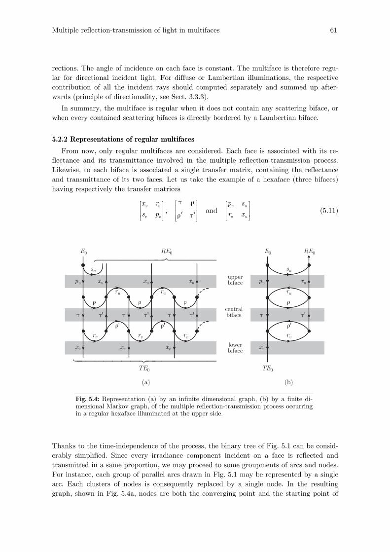
Multiple reflection-transmission of light in multifaces 61
rections. The angle of incidence on each face is constant. The multiface is therefore regu-lar for directional incident light. For diffuse or Lambertian illuminations, the respective contribution of all the incident rays should computed separately and summed up after-wards (principle of directionality, see Sect. 3.3.3).
In summary, the multiface is regular when it does not contain any scattering biface, or when every contained scattering bifaces is directly bordered by a Lambertian biface.
5.2.2 Representations of regular multifaces
From now, only regular multifaces are considered. Each face is associated with its re-flectance and its transmittance involved in the multiple reflection-transmission process. Likewise, to each biface is associated a single transfer matrix, containing the reflectance and transmittance of its two faces. Let us take the example of a hexaface (three bifaces) having respectively the transfer matrices
v v
v v
x r
s p⎡ ⎤⎢ ⎥⎢ ⎥⎣ ⎦
, τ ρ⎡ ⎤
⎢ ⎥⎢ ⎥′ ′ρ τ⎢ ⎥⎣ ⎦
and u u
u u
p s
r x⎡ ⎤⎢ ⎥⎢ ⎥⎣ ⎦
(5.11)
su
RE0
TE0
xv
τ
pu
E0
xv
pu
xv
ρ
ρ'
ττ'
rv
xu
ru
E0
TE0
RE0
ρ
ρ'
τ τ'
rv
xu
ru
su
xv
ρ
ρ'
ττ'
rv
xu
ru
ρ
τ'
rv
xu
upperbiface
centralbiface
lowerbiface
(a) (b)
Fig. 5.4: Representation (a) by an infinite dimensional graph, (b) by a finite di-mensional Markov graph, of the multiple reflection-transmission process occurring in a regular hexaface illuminated at the upper side.
Thanks to the time-independence of the process, the binary tree of Fig. 5.1 can be consid-erably simplified. Since every irradiance component incident on a face is reflected and transmitted in a same proportion, we may proceed to some groupments of arcs and nodes. For instance, each group of parallel arcs drawn in Fig. 5.1 may be represented by a single arc. Each clusters of nodes is consequently replaced by a single node. In the resulting graph, shown in Fig. 5.4a, nodes are both the converging point and the starting point of

62 Chapter 5
arcs. They represent both the collecting and the splitting of irradiance components. In such a graphical representation, the development of the multiple reflection-transmission process in time is preserved, but the graph is infinite dimensional.
An even more compact representation is possible, although the visual representation of time is lost. All the arcs relative to a same reflection or transmission are grouped into a single arc. A finite graph is obtained, with only one reflection arc and one transmission arc per face (Fig. 5.4b). Since the values of arc weights are all percentages, such a graph is analogous to the graphical representation of a Markov chain.
The analogy between multiple reflection-transmission processes and Markov chains is highly profitable for our compositional model. We will take benefit of the well established mathematical methods embodied into the so-called Markov theory for establishing the formulae for multiface global reflectances and transmittances. The Markov matrix formal-ism has inspired us the idea of endowing also our compositional theory with a matrix-like formalism. Pursuing this idea, we now introduce a well-defined “product” of transfer ma-trices, called composition (notation ), permitting to visualize under an algebraic form the superposition of bifaces in regular multifaces. Hence, the synthetic view of the light transfer process provided by the Markov graph is doubled by an algebraic equation that we call composition equation.
Consider a multiface with global transfer matrix G, resulting from the superposition of a biface having the transfer matrix F1 on the upper side and a biface having the transfer matrix F2 on the lower side. The corresponding composition equation is written as
G = F1 F2 (5.12)
For example, the composition equation corresponding to the hexaface of Fig. 5.4 is
U U u u v v
u u v vV V
T R p s x r
r x s pR T
τ ρ⎡ ⎤ ⎡ ⎤⎡ ⎤ ⎡ ⎤⎢ ⎥ ⎢ ⎥⎢ ⎥ ⎢ ⎥=⎢ ⎥ ⎢ ⎥′ ′⎢ ⎥ ⎢ ⎥ρ τ⎣ ⎦ ⎣ ⎦⎢ ⎥⎢ ⎥ ⎣ ⎦⎣ ⎦ (5.13)
Note that the position of transfer matrices with respect to symbol has an importance. The composition operation is not commutative. The definition of will be given in Sect. 5.3.1 by the expressions for TU, RU, TV and RV as functions of the face reflectances and transmittances. Let us now present the Markov chains that will permit the efficient computation of these expressions.
5.2.3 Analogy between regular multifaces and Markov chains
A Markov chain is a convenient representation of the behavior of a physical system which describes the different states the system may occupy and indicates how the system moves from one state to another in time [Ste94]. Our conception of time has already been described in Sect. 5.1.1. In the context of multiple reflection-transmission processes, the system is the multiface. The different states occupied by the system are the incidence of light on the different faces. A path, i.e. a succession of reflections and transmissions, is represented by a succession of state-to-state transitions within the chain. Reflectances and transmittances become probabilities of transition. Table 5.1 completes the correspondence between multiple reflection-transmission processes and Markov chains.

Multiple reflection-transmission of light in multifaces 63
Table 5.1: Correspondence between concepts underlying multiple reflection-transmission processes and
Markov chains.
Multiface
Light reaching a face or a detector
Reflection / transmission
Reflectance / transmittance
Time-dependent process
Time-independent process
External faces
Structured stochastic system
State
Transition
Transition probability
Time-dependent stochastic process
Homogenous Markov chain
Ephemeral or absorbing states
A survey of basic definitions and results of Markov theory is proposed in Appendix B. Let us recall here that a stochastic process can be represented by a Markov chain only when every state-to-state transition has a time-independent probability to occur. There-fore, the Markov theory can be used only with regular multifaces.
Lower biface
SourceDetector
1 7 2
Upper biface
Source Detector
3 4
5 2
1 16
Fig. 5.5: Markov graph for a regular quadriface.
Consider a multiface having N faces, two light sources (one in each surrounding me-dium) and two detectors (idem). The N faces and the two detectors, each one able to receive light, are the N + 2 states of our system. They are labeled with a number between 1 and N + 2 according to the following convention1 (see Fig. 5.5):
− Numbers 1 and 2 are associated to the states corresponding to the external faces, which receive light from the light sources (most external faces). Since they receive light only once at the time origin, they are ephemeral states;
− Numbers N + 1 and N + 2 are associated to the detectors. A loop connecting these states to themselves modelizes the fact that light captured by the detectors does no longer interfere with the bifaces. States 5 and 6 are absorbing states. We are therefore in pres-ence of absorbing Markov chains (see Appendix B.4);
⎯⎯⎯⎯⎯⎯⎯⎯⎯⎯⎯ 1 All distributions of state labels are equivalent. We are therefore free to choose the more conven-ient one according to computational considerations.
64 Chapter 5
− Odd numbers (resp. even numbers) are attributed to the states receiving the light propagating downwards (res. upwards). Odd numbers increase and even numbers decrease as the states are closer to the lower side.
Let be mij the probability of transition from state i to state j. Matrix ( )ijm=M is called the single-step transition probability matrix of the Markov chain. We note ( )k
ijm the probability that a transition takes place from state i to state j in k steps. Probabilities
( )kijm are placed in a k-step transition probability matrix M(k). The k-step and single-step
matrices are linked by the simple relation (see Eqs. (B.7) to (B.9) in Appendix B.2)
( )k k=M M (5.14)
We are interested in the global reflectances and transmittances of the multiface. They correspond to the probability that the incident irradiance transits from a source to a de-tector, whatever the number of steps. Let 1, 1Nm∞
+ , 1, 2Nm∞+ , 2, 1Nm∞
+ and 2, 2Nm∞+ be the transi-
tion probabilities corresponding to the four possible source-detector combinations. They are elements of the “infinite-step” transition probability matrix ( )ijm∞
∞ =M defined as
lim k
k∞ →∞
=M M (5.15)
The relationship between matrix ∞M and the global transfer matrix of a multiface will be appear clearly with the simple example of a quadriface below.
5.3 Compositional model for regular multifaces
We just saw that the global transfer matrix of a regular multiface is a part of the infi-nite-step transition probability matrix associated with a Markov chain. Let us consider generic multifaces: a quadriface (two superposed bifaces), a hexaface (three superposed bifaces) and a N-dimensional multiface. For each case, by establishing the Markov chain and its associated single step probability matrix, and then by computing the infinite step transition probability matrix, we will obtain the global transfer matrix of the considered multiface. The obtained expressions, called “compositional formulae” will correspond to the definition of operation .
5.3.1 The quadriface formula
Let us consider the regular quadriface represented by the 6-states Markov chain in Fig. 5.6 and by the following composition equation
U U u u v v
u u v vV V
T R p s x r
r x s pR T
⎡ ⎤ ⎡ ⎤ ⎡ ⎤⎢ ⎥ ⎢ ⎥ ⎢ ⎥=⎢ ⎥ ⎢ ⎥ ⎢ ⎥⎣ ⎦ ⎣ ⎦⎢ ⎥⎣ ⎦ (5.16)
The single-step transition probability matrix M of the chain is obtained by placing the nonzero probabilities mij indicated in Fig. 5.6. For example, the probability pu of transi-tion from state 1 to state 3 is placed in row 1, column 3. Once all the elements featured in the graph are placed, M is filled with zeros

Multiple reflection-transmission of light in multifaces 65
lower biface
lowersource
lowerdetector
1
rv
svxv pv
7 2
upper biface
uppersource
upperdetector
ru
su xupu
3 4
5 2
1 16
Fig. 5.6: Graph representing the multiple reflection-transmission process in a regular quadriface.
=M
0 0 0 00 0 0 00 0 0 00 0 0 00 0 0 0 1 00 0 0 0 0 1
u u
v v
v v
u u
p sp sr x
r x
⎡ ⎤⎢ ⎥⎢ ⎥⎢ ⎥⎢ ⎥⎢ ⎥⎢ ⎥⎢ ⎥⎢ ⎥⎢ ⎥⎢ ⎥⎢ ⎥⎢ ⎥⎢ ⎥⎢ ⎥⎢ ⎥⎢ ⎥⎢ ⎥⎢ ⎥⎢ ⎥⎣ ⎦
(5.17)
The location of light in time may be observed using a probability vector. We will use bold characters for the two last elements, which represent the amounts of light having reached the lower and the upper detectors respectively. Let us first consider that the incident light comes from the upper light source. At time origin, all light is in state 1, i.e. is incident on the upper face of the upper biface (see Fig. 5.6). The probability vector is
[ ]0 1, 0, 0, 0, , =e 0 0 (5.18)
At time 1, the location of light within the quadriface is given by the product 0 ⋅e M
[ ]1 0 0, 0, , 0, , up= ⋅ =e e M 0 us
A fraction su (external reflectance of the upper biface) of the incident light has already reached the upper detector. At time 2, the product 1 ⋅e M shows that a fraction puxv has reached the lower detector
[ ]22 1 0 0, 0, 0, , , u vp r= ⋅ = ⋅ =e e M e M u v up x s
At time 3, the probability vector is
[ ]33 2 0 0, 0, , 0, , u u vp r r= ⋅ = ⋅ = +e e M e M u v u u v up x s p r x
Matrices M2 and M3 are respectively the two-step and the three-step transition probabil-ity matrices. One retrieves, with this short description, the general property (5.14) satis-fied by transition probability matrices.
Pursuing the products of the probability vector by matrix M, one would observe that

66 Chapter 5
the proportion of light reaching the detectors increases and that the proportion of light remaining in other states decreases. At the “end” of the process, there is no remaining light within the multiface. The probability 15m∞ for the incident light to be captured by the lower detector corresponds to the upper global transmittance. Likewise, the proability
15m∞ to be captured by the upper detector corresponds to its upper global reflectance
[ ]0 15 160, 0, 0, 0, , ∞ ∞∞ ∞= ⋅ =e e M m m (5.19)
Let us now consider that light comes from the lower source. At time origin, the probabil-ity vector e0 is
[ ]0 0, 1, 0, 0, , =e 0 0 (5.20)
By multiplying this vector by matrix M an infinite number of times, or by multiplying it by ∞M , which is equivalent, we would obtain a probability vector indicating once again that there is no remaining light within the multiface
[ ]0 25 260, 0, 0, 0, , ∞ ∞∞ ∞= ⋅ =e e M m m (5.21)
In (5.21), 25m∞ and 26m∞ correspond respectively to the lower global reflectance and transmittance of the quadriface. In Appendix B, we show that the chains representing multiple reflection-transmission processes are such that matrix M∞ is of the form
15 16
25 26
0 0 0 0
0 0 0 0
0 0 0 0
0 0 0 0
0 0 0 0 1 0
0 0 0 0 0 1
m m
m m
∞ ∞
∞ ∞
∞
⎡ ⎤⎢ ⎥⎢ ⎥⎢ ⎥⎢ ⎥⋅ ⋅⎢ ⎥= ⎢ ⎥⋅ ⋅⎢ ⎥⎢ ⎥⎢ ⎥⎢ ⎥⎢ ⎥⎣ ⎦
M (5.22)
where the upper-right block corresponds to the global transfer matrix of the multiface
15 16
25 26
U U
V V
T R m m
R T m m
∞ ∞
∞ ∞
⎡ ⎤⎡ ⎤⎢ ⎥⎢ ⎥ = ⎢ ⎥⎢ ⎥⎢ ⎥⎢ ⎥⎣ ⎦ ⎣ ⎦
(5.23)
The computation of the upper-right block for the case of the quadriface is developed in Appendix C.1. The resulting expression for the global transfer matrix is
1 1
1 1
u v u u vu
U U u u v v u v u v
u u v v v v u v uV Vv
u v u v
p x p x rsT R p s x r r r r r
r x s p p x r p xR T sr r r r
⎡ ⎤+⎢ ⎥⎡ ⎤ ⎡ ⎤ ⎡ ⎤ − −⎢ ⎥⎢ ⎥ ⎢ ⎥ ⎢ ⎥= = ⎢ ⎥⎢ ⎥ ⎢ ⎥ ⎢ ⎥ ⎢ ⎥⎣ ⎦ ⎣ ⎦⎢ ⎥ +⎣ ⎦ ⎢ ⎥− −⎣ ⎦
(5.24)
Eq. (5.24) will be referred to as the quadriface formula. It corresponds to the definition of the composition symbol as a (noncommutative) operation between transfer matrices. It is the most fundamental equation of the compositional model.

Multiple reflection-transmission of light in multifaces 67
5.3.2 The hexaface formula
Let us now consider a regular hexaface, resulting from the superposition of three bi-faces, called upper, central and lower. It is represented by the 8 states graph of Fig. 5.7 and by the composition equation
UV UU u u v v
u u v vVV VU
T R p s x r
r x s pR T
τ ρ⎡ ⎤ ⎡ ⎤⎡ ⎤ ⎡ ⎤⎢ ⎥ ⎢ ⎥⎢ ⎥ ⎢ ⎥=⎢ ⎥ ⎢ ⎥′ ′⎢ ⎥ ⎢ ⎥ρ τ⎣ ⎦ ⎣ ⎦⎢ ⎥⎢ ⎥ ⎣ ⎦⎣ ⎦ (5.25)
lowerbiface
upperbiface
centralbiface
uppersource
lowersource
lowerdetector
upperdetector
1
ρρ'
ru
rv
su
sv
xupu
xv pv
τ τ'
3 6
5 4
1 18
7 2
Fig. 5.7: Representation by a Markov graph of the multiple reflection-transmission occurring with three superposed bifaces.
Like for the quadriface, the global transfer matrix of the hexaface is the upper-right block of the infinite-step transition probability matrix M∞ defined by Eq. (5.15) with the fol-lowing single-step transition probability matrix M
=M
0 0 0 0 0 00 0 0 0 0 00 0 0 0 0 0
0 0 0 0 0 00 0 0 0 0 00 0 0 0 0 00 0 0 0 0 0 1 00 0 0 0 0 0 0 1
u u
v v
v v
u u
p sp s
r xr x
⎡ ⎤⎢ ⎥⎢ ⎥⎢ ⎥⎢ ⎥⎢ ⎥⎢ ⎥⎢ ⎥⎢ ⎥⎢ ⎥⎢ ⎥⎢ ⎥⎢ ⎥⎢ ⎥⎢ ⎥⎢ ⎥⎢ ⎥⎢ ⎥⎢ ⎥⎢ ⎥⎢ ⎥⎢ ⎥⎢ ⎥⎢ ⎥⎢ ⎥⎢ ⎥⎢ ⎥⎣ ⎦
τ ρ′ ′ρ τ
(5.26)
M presents a cross structure that was already noticeable in (5.17).
The computation of the upper-right block of M∞ is developed in Appendix C.2. It yields the following equation, which will be referred to as the hexaface formula

68 Chapter 5
( )
( )
U U u u v v
u u v vV V
vu v u u u
uv v v v u
T R p s x r
r x s pR T
rp x s p x
D Dr
s p x p xD D
τ ρ⎡ ⎤ ⎡ ⎤⎡ ⎤ ⎡ ⎤⎢ ⎥ ⎢ ⎥⎢ ⎥ ⎢ ⎥=⎢ ⎥ ⎢ ⎥′ ′⎢ ⎥ ⎢ ⎥ρ τ⎣ ⎦ ⎣ ⎦⎢ ⎥⎢ ⎥ ⎣ ⎦⎣ ⎦⎡ ⎤′ ′ρ − ρρ − τττ⎢ ⎥+⎢ ⎥⎢ ⎥= ⎢ ⎥′ ′ ′ρ − ρρ − ττ ′τ⎢ ⎥+⎢ ⎥⎣ ⎦
(5.27)
with ( )( )1 1u v u vD r r r r′ ′= − ρ − ρ − ττ .
5.3.3 Associativity of the composition of bifaces
The hexaface formula can also be obtained using twice the quadriface formula. First, two adjacent bifaces are selected within the hexaface and merged into a single biface, whose global transfer matrix is expressed using the quadriface formula. Then, the quadri-face formula is applied again to this resulting biface and the third biface, leading to the global transfer matrix of the hexaface. We may compose first the left and the central transfer matrices
1 1
1 1
u u uu
u u v v v vu u
u u v v v vu u
u u
p p xs
p s x r x rr rr x s p s pr x
r r
τ ρ⎡ ⎤+⎢ ⎥τ ρ⎧ ⎫⎡ ⎤ − ρ − ρ⎪ ⎪⎡ ⎤ ⎡ ⎤ ⎡ ⎤⎢ ⎥⎪ ⎪⎪ ⎪⎢ ⎥⎢ ⎥ ⎢ ⎥ ⎢ ⎥⎢ ⎥=⎨ ⎬⎢ ⎥′ ′ ′ ′⎢ ⎥ ⎢ ⎥ ⎢ ⎥ρ τ ττ τ⎪ ⎪ ⎢ ⎥⎣ ⎦ ⎣ ⎦ ⎣ ⎦⎢ ⎥⎪ ⎪ ′⎣ ⎦ ρ +⎪ ⎪⎩ ⎭ ⎢ ⎥⎢ − ρ − ρ ⎥⎣ ⎦
(5.28)
or compose first the central and the right transfer matrices
1 1
1 1
v v
u u v v u u v v
u u v v u u v v vv
v v
x rp s x r p s r rr x s p r x p x p
sr r
⎡ ⎤′τ ττ⎢ ⎥ρ +τ ρ⎧ ⎫⎡ ⎤ ⎢ ⎥⎪ ⎪⎡ ⎤ ⎡ ⎤ ⎡ ⎤ − ρ − ρ⎪ ⎪⎪ ⎪⎢ ⎥ ⎢ ⎥⎢ ⎥ ⎢ ⎥ ⎢ ⎥=⎨ ⎬⎢ ⎥ ⎢ ⎥′ ′⎢ ⎥ ⎢ ⎥ ⎢ ⎥ρ τ⎪ ⎪ ′ ′ρ τ⎣ ⎦ ⎣ ⎦ ⎣ ⎦⎢ ⎥⎪ ⎪ ⎢ ⎥⎣ ⎦⎪ ⎪⎩ ⎭ +⎢ ⎥− ρ − ρ⎣ ⎦
(5.29)
and check that in both cases the final transfer matrix is identical to Eq. (5.27). This shows the associativity of operation . For transfer matrices F1, F2 and F3, one has
( ) ( )1 2 3 1 2 3 1 2 3= =F F F F F F F F F (5.30)
5.3.4 Composition formula for more than two bifaces
We now consider a regular multiface composed of k bifaces. The corresponding Markov chain has 2k+2 states (Fig. 5.8), numbered according to the labeling convention presented in Sect. 5.2.3. The single-step matrix M has the cross structure that has already been pointed out (the empty spaces should be considered as filled with zeros)

Multiple reflection-transmission of light in multifaces 69
M =
1 1
2 2
2 2
1 1
1
1
k k
k k
⎡ ⎤⎢ ⎥⎢ ⎥⎢ ⎥⎢ ⎥⎢ ⎥⎢ ⎥⎢ ⎥⎢ ⎥⎢ ⎥⎢ ⎥⎢ ⎥⎢ ⎥⎢ ⎥⎢ ⎥⎢ ⎥⎢ ⎥⎢ ⎥⎢ ⎥⎢ ⎥⎢ ⎥⎢ ⎥⎢ ⎥⎢ ⎥⎢ ⎥⎢ ⎥⎢ ⎥⎢ ⎥⎢ ⎥⎢ ⎥⎢ ⎥⎢ ⎥⎢ ⎥⎢ ⎥⎢ ⎥⎢ ⎥⎢ ⎥⎢ ⎥⎢ ⎥⎢ ⎥⎣ ⎦
τ ρ
′ ′τ ρ
τ ρ
′ ′ρ τ
ρ τ
′ ′ρ τ
(5.31)
3rd biface
1st biface
2nd bifaceρ2
ρ'2
τ2 τ'2
ρ1
ρ'1
τ1 τ'1
ρk
ρ'k
τk τ'k
ρ3
ρ'3
τ3 τ'3
ρk-1
ρ'k-1τk-1 τ'k-1
3 2k
5 2k − 2
1 12k +2
7 2k − 4
kth biface
1
4
(k −1)th biface
2k − 3 6
2k +1 2
2k −1
Fig. 5.8: Markov graph representing the multiple reflection-transmission process within k superposed bifaces.
Let Gj and Fj+1 be respectively the transfer matrices of j successive bifaces and of a (j+1)th biface. At iteration j, the composition of Gj and Fj+1 is
( )1
1
1
1, 2, ..., 1
j j
j
j j
or j k
+
+
+
= = −
G F
GF G
(5.32)
according to whether the (j+1)th biface is at the upper or resp. at the lower side of the j first bifaces. Denoting by Rj, Tj, jR′ and jT ′ the components of Gj, the composition with

70 Chapter 5
the (j+1)th biface at the lower side, given by the quadriface formula (5.32), gives the fol-lowing iterative formula, called the composition formula
1 1
1 11 1 1 1
1 11 1 1 1 11
1 1
1 1
1 1
j j j j jj
j jj j j j j j j j
j jj j j j j j j j jj
j j j j
T T TRT R T R R R
R T R T R T
R R
+ +
+ ++ + + +
+ ++ + + + ++
+ +
⎡ ⎤′τ ρ⎢ ⎥+τ ρ ⎢ ⎥⎡ ⎤ ⎡ ⎤ ⎡ ⎤ ′ ′− ρ − ρ⎢ ⎥⎢ ⎥ ⎢ ⎥ ⎢ ⎥= = ⎢ ⎥⎢ ⎥ ⎢ ⎥ ⎢ ⎥′ ′ρ τ′ ′ ′ ′ ′ ′ ′ ′τ τ τ⎢ ⎥⎢ ⎥ ⎢ ⎥ ⎢ ⎥⎣ ⎦⎣ ⎦ ⎣ ⎦ ′ρ +⎢ ⎥′ ′− ρ − ρ⎢ ⎥⎣ ⎦
(5.33)
5.4 Biface splitting
In compositional models, it is sometimes judicious to dissociate the different compo-nents of the transfer matrix characterizing a biface. Imagine two layers separated by an interface. We would like to compose the interface’s upper face with the upper layer, and to compose its lower face with the lower layer. Since composition can be performed only with transfer matrices, we propose to characterize the interface with two transfer matri-ces. The interface becomes a quadriface having the same global transfer matrix as the original biface. We call this procedure “biface splitting”.
Graphically, the split is performed like in Fig. 5.9. The upper (resp. lower) reflection arc is placed at the upper side of the upper biface (resp. the lower side of the upper bi-face). The other reflections arcs have a zero reflectance. The left (resp. right) transmission arc is placed at the left (resp. right) of the quadriface; we may choose to place it on the upper or the lower biface, the other left arc (resp. right arc) having the transmittance 1. Fig. 5.9 features two of the four split possibilities.
⇔
a
10
b
1
dc
0
⇔
1 10
b
a d
c
0
ad
c
b
Fig. 5.9: Two possible splits of a biface.
We may write the following composition equations for the splits illustrated in Fig. 5.9, and check, thanks to the quadriface formula (5.24), the equality between the transfer ma-trix of the original biface and the global transfer matrices of the quadrifaces issued from the split operations
01 0 1
0 1 0 1
aa b a b b
c dc dc d
⎡ ⎤ ⎡ ⎤ ⎡ ⎤ ⎡ ⎤ ⎡ ⎤⎢ ⎥ ⎢ ⎥ ⎢ ⎥ ⎢ ⎥ ⎢ ⎥= =⎢ ⎥ ⎢ ⎥ ⎢ ⎥ ⎢ ⎥ ⎢ ⎥⎢ ⎥ ⎢ ⎥ ⎢ ⎥ ⎢ ⎥ ⎢ ⎥⎣ ⎦⎣ ⎦ ⎣ ⎦ ⎣ ⎦⎣ ⎦
(5.34)

Multiple reflection-transmission of light in multifaces 71
Summary
In this chapter, we have described the multiple reflection-transmission process occur-ring in multifaces, first in the general case where the multiface global reflectance and transmittance are expressed as infinite sums, and then in the special case of regular multi-faces whose global reflectance and transmittance have analytical expressions. The criteria of regularity have been clearly stated: the multiface is regular when it does not contain any scattering biface, or when every contained scattering biface is directly bordered by Lambertian bifaces. In regular multifaces, each face has a constant reflectance and a con-stant transmittance. This allows representing the multiple reflection-transmission process by a Markov chain. Bifaces also have a constant transfer matrix. Thus, the superposition of bifaces can now be characterized by a “composition” of their respective transfer matrix, i.e. by a well-defined associative and noncommutative product. We have presented, thanks to mathematical tools embodied in the Markov theory, a closed-form defining ex-pression for the composition of two and three transfer matrices, characterizing the super-position of two and three bifaces respectively. These defining expressions are called the “quadriface formula” and the “hexaface formula”. For more superposed bifaces, the quadriface or/and the hexaface formulae can be applied iteratively.
The compositional formulae rely only on the assumption that the multiface is regular, i.e. that each face has a single reflectance and a single transmittance involved in the mul-tiple reflection-transmission process. In the next chapter, we show how these face reflec-tances and transmittances can be determined, given a particular combination of super-posed bifaces, and a given measuring geometry. This will allow a revisitation of some clas-sical models, as well as the development of new models in Chapters 7 and 8.
Note that the introduction of Markov chains was not strictly necessary. We could have derived the quadriface formula using a step-by-step description, and compose this formula with itself for obtaining the hexaface formula and the compositional formula. However, we have intentionally used the Markov theory for the elegance and the efficiency of its ma-trix formalism. Markov graphs are excellent representations of multiple reflection-transmission process within multilayers. Another reason for introducing Markov chains is the idea of a possible extension to multilayers having an unknown structure, i.e. an un-known number of layers and interfaces. By combining our compositional model with the theory of hidden Markov chains, we may obtain a new noninvasive method for studying multilayer specimens.


73
Chapter 6.
Reflectance and transmittance models
The present chapter concerns the application of the composition formulae established in Chapter 5 to specified multifaces. We first present how, for a given multiface, the reflectance and the transmittance of each of its face shall be determined. The nature of the faces (transparent, scattering, Lambertian), their neighborhood and the meas-uring geometry will be taken into account (Sect. 6.1). Then, classical compositional models and some of their extensions will be presented as examples where our formal-ism may be applied. Their expressions for reflectance, respectively transmittance, are derived by the simple application of the compositional formulae. We first treat multi-faces composed uniquely of transparent bifaces and of Lambertian multifaces (Sect. 6.2). Then, we consider the superposition of transparent bifaces on a Lamber-tian background with three examples, including the well-known Williams-Clapper model (Sect. 6.3).
6.1 Elaboration of a reflectance and transmittance model
We have shown in Chapter 5 that the multiple reflection-transmission process of light occurring in a regular multiface can be described with a single reflectance and a single transmittance per face. Thus, a particular transfer matrix is associated to each biface, and the multiface is characterized by the composition of the particular transfer matrices of its composing bifaces. The quadriface and the hexaface formulae can be applied to convert the composition of biface transfer matrices into a global transfer matrix. However, we have not yet explained the reflectance and transmittance that should be associated with each face. This is the purpose of the following sections.
Two main factors should be taken into account in the specification of the face reflec-tances and transmittances: 1- the nature of the face (transparent, scattering, Lamber-tian), 2- their neighborhood, which determines the type of their respective illumination (transparent, scattering, Lambertian neighboring faces respectively provide a directional, diffuse, Lambertian illumination). A special treatment is necessary for external bifaces due to the influence of th
e selected measuring geometry.
Prior to the specification of the face reflectances and transmittances, let us draw up a brief inventory of the possible combinations of bifaces forming regular multifaces.
6.1.1 Types of regular bifaces
Regular bifaces may be split into three main categories:
− Transparent multifaces, made uniquely of transparent bifaces. All the face reflectances and transmittances are, directly or indirectly via Snell’s laws, functions of the incidence

74 Chapter 6
angle of the directional source light (principle of directionality, see Sect. 3.3.3).
− Wholly-Lambertian multifaces, composed uniquely of Lambertian bifaces1. The faces reflectances and transmittances are invariant, excepted for the external biface whose ex-ternal reflectance and exit transmittance (i.e. the terms corresponding to the transfer of light towards the capturing device) depend on the geometry of observation;
− Mixed multifaces, in which Lambertian bifaces are superposed with scattering or/and transparent bifaces. Recall that scattering bifaces cannot be bordered by scattering nor reflecting transparent bifaces: the regularity would not be satisfied (Sect. 5.2.1).
6.1.2 Faces reflectances and transmittances in mixed multifaces
In mixed multifaces, the bifaces may be transparent, scattering or/and Lambertian. Lambertian bifaces are characterized by their invariant transfer matrix FL. Non-Lambertian bifaces, i.e. transparent and scattering bifaces, are characterized by their fun-damental transfer matrix Fθ. In the present section, matrices FL and Fθ are noted respec-tively
L L
LL L
p s
r x⎡ ⎤⎢ ⎥= ⎢ ⎥⎣ ⎦
F and ( ) ( )
( ) ( )
P S
R Xθ
⎡ ⎤θ θ⎢ ⎥= ⎢ ⎥θ θ⎢ ⎥⎣ ⎦F (6.1)
The specification of the face reflectances and transmittances is performed in a different way for central bifaces and for external bifaces, the latter being affected by the measuring geometry (Fig 6.1).
External biface
Central bifacesρ
ρ'
r
s xp
τ τ'
Terms depending on the illumination geometry
Terms depending on theobservation geometry
Upper source(ephemeral state)
Upper detector(absorbing state)
Fig. 6.1: Dependence of external biface reflectances and transmittances on the il-lumination and observation geometries.
⎯⎯⎯⎯⎯⎯⎯⎯⎯⎯⎯ 1 Wholly-Lambertian multifaces are special cases of Lambertian multifaces, according to the defini-tion of Lambertian multiface given in Section 2.4.

Reflectance and transmittance models 75
When a Lambertian biface is at a central position within the multiface, its particular transfer matrix is the matrix FL given by Eq. (6.1). A central biface that is non-Lambertian is bordered by Lambertian bifaces, and therefore receives Lambertian illumi-nations on its both sides. According to the notations introduced in Sect. 2.3, its funda-mental transfer matrix Fθ, given in Eq. (6.1), becomes the particular transfer matrix
( ) ( )
( ) ( )
( ) ( )
( ) ( )
/2 /2
0 0/2 /2
0 0
sin2 sin2
sin2 sin2
L
L
T d R dT R
R T R d T d
π π→
θ= θ=π π
←θ= θ=
⎡ ⎤⎡ ⎤ θ θ θ θ θ θθ θ ⎢ ⎥⎢ ⎥ ⎢ ⎥=⎢ ⎥ ⎢ ⎥′ ′θ θ⎢ ⎥ ⎢ ⎥′ ′θ θ θ θ θ θ⎣ ⎦ ⎢ ⎥⎣ ⎦
∫ ∫
∫ ∫ (6.2)
Let us now study the external bifaces1. We will consider here the upper external biface, the lower external biface being characterized equivalently with reversed notations. As stated in Sect. 2.4, every external biface is represented by a particular transfer matrix of the form
p s
r x⎡ ⎤⎢ ⎥⎢ ⎥⎣ ⎦
(6.3)
where p is the penetration transmittance, s the external reflectance, r the internal reflec-tance and x the exit transmittance.
These four terms are determined according to the nature of the biface and the measur-ing geometry. Table 6.1 (see next page) draws up the inventory of particular transfer ma-trices considering the different types of biface (transparent, scattering, Lambertian), of light source (directional or Lambertian light source) and of capturing device (integrating sphere, radiance detector). The complete statement of these particular transfer matrices is presented in Appendix D.
6.1.3 Standard procedure for the development of a model
All the elements are now available for expressing the global reflectance and transmit-tance of any regular multiface:
1. Verify whether the superposed bifaces form a regular multiface, i.e. check that there is no succession of scattering bifaces or whether the contained scattering bifaces are di-rectly bordered by Lambertian bifaces (Sect. 5.2.1).
2. Group consecutive transparent bifaces if any. Their fundamental transfer matrix can be obtained using the compositional formulae.
3. Determine the particular transfer matrix of each central biface according to its illumi-nation, and of each external biface according to the measuring geometry, by referring to Table 6.1.
4. Write the composition equation with these particular transfer matrices. Apply the appropriate compositional formula(e) and derive the global transfer matrix of the mul-tiface.
⎯⎯⎯⎯⎯⎯⎯⎯⎯⎯⎯ 1 An external biface may be a single interface (see Sect. 6.3.1), the superposition of flat interfaces and transparent layers (see Sect. 6.3.2 and 6.3.3), a rough interface as in matte opaque paints, a Lambertian layer, as in uncombed woolen or cotton fabrics, etc.

76 Chapter 6
Table 6.1: Transfer matrix of the upper external biface specified according to the type of biface,
the type of light source and the type of capturing device.
Integrating sphere Radiance detector
Lambertian external biface
(a) any
L L L L
L L L Lsph any
p s p s
r x r x
→
← ←
⎡ ⎤ ⎡ ⎤⎢ ⎥ ⎢ ⎥=⎢ ⎥ ⎢ ⎥⎣ ⎦ ⎣ ⎦
(b) ( )
/
/
anyL L L L
L L L Lrad any
p s p s
r x r x
→
′ψ ← ←
⎡ ⎤ξ π⎡ ⎤ ⎢ ⎥⎢ ⎥ = ⎢ ⎥⎢ ⎥ ξ π⎢ ⎥⎣ ⎦ ⎣ ⎦
Scattering external biface
Directional light source
(c)
( ) ( ) ( )
( ) ( )
( ) ( )dir
sph L
P SP S
R X R X
ψ →
← ←
⎡ ⎤ψ ψ⎡ ⎤θ θ ⎢ ⎥⎢ ⎥ = ⎢ ⎥⎢ ⎥θ θ ⎢ ⎥⎢ ⎥⎣ ⎦ ⎢ ⎥⎣ ⎦∫ ∫ (d)
( )
( ) ( ) ( )
( ) ( )
( ) ( )
( )
,dirR
Trad L
P fP S
R X R f
ψ →
′ψ ← ←
⎡ ⎤′ψ ξ ψ ψ⎡ ⎤θ θ ⎢ ⎥⎢ ⎥ = ⎢ ⎥⎢ ⎥ ⎢ ⎥θ θ ′ξ ψ⎢ ⎥⎣ ⎦ ⎢ ⎥⎣ ⎦∫ ∫∫
Lambertian light source
(e) ( ) ( )
( ) ( )
L
sph L
P SP S
R X R X
→
← ←
⎡ ⎤⎡ ⎤θ θ ⎢ ⎥⎢ ⎥ ⎢ ⎥=⎢ ⎥ ⎢ ⎥θ θ⎢ ⎥ ⎢ ⎥⎣ ⎦ ⎣ ⎦
∫ ∫∫ ∫
(f) ( )
( ) ( )
( ) ( )
( )
( )
LR
Trad L
P fP S
R X R f
→
′ψ ← ←
⎡ ⎤′⎡ ⎤ ξ ψθ θ ⎢ ⎥⎢ ⎥ ⎢ ⎥=⎢ ⎥ ⎢ ⎥θ θ ′⎢ ⎥ ξ ψ⎢ ⎥⎣ ⎦ ⎣ ⎦
∫ ∫∫∫ ∫∫
Transparent external biface
Directional light source
(g)
( ) ( ) ( )
( ) ( )
( ) ( )dir
sph L
P SP S
R X R X
ψ →
← ←
⎡ ⎤ψ ψ⎡ ⎤θ θ ⎢ ⎥⎢ ⎥ = ⎢ ⎥⎢ ⎥θ θ ⎢ ⎥⎢ ⎥⎣ ⎦ ⎢ ⎥⎣ ⎦∫ ∫ (h)
( )
( ) ( ) ( )
( ) ( )
( )
( )( )
12
1 0
0
/
dir
rad L
PP S
XR X R
n n
ψ →
′ψ ← ←
⎡ ⎤ψ⎢ ⎥⎡ ⎤θ θ ⎢ ⎥⎢ ⎥ = ′ξ ψ⎢ ⎥⎢ ⎥θ θ ⎢ ⎥⎢ ⎥⎣ ⎦ ⎢ ⎥π⎣ ⎦∫
Lambertian light source
(i) ( ) ( )
( ) ( )
L
sph L
P SP S
R X R X
→
← ←
⎡ ⎤⎡ ⎤θ θ ⎢ ⎥⎢ ⎥ ⎢ ⎥=⎢ ⎥ ⎢ ⎥θ θ⎢ ⎥ ⎢ ⎥⎣ ⎦ ⎣ ⎦
∫ ∫∫ ∫
(j) ( )
( ) ( )
( ) ( )
( )( )
( )
12
1 0
/
/
L
rad L
P SP S
XR X Rn n
→
′ψ ← ←
⎡ ⎤′ξ ψ π⎢ ⎥⎡ ⎤θ θ ⎢ ⎥⎢ ⎥ = ⎢ ⎥′ξ ψ⎢ ⎥ ⎢ ⎥θ θ⎢ ⎥⎣ ⎦ ⎢ ⎥π⎢ ⎥⎣ ⎦
∫
∫
Legend: The left matrices are invariant or fundamental transfer matrices [see Eq. (6.1)], with specifi-cation of the upper illumination (left superscript), the lower illumination (right subscript), and thecapturing device (left subscript). Symbol L stands for “Lambertian”, dir(ψ) for “directional with incident angle ψ”, rad(ψ′′) for “radiance detector with observation angle ψ′′” and sph for “integrating sphere”. Notation g∫ stands for ( )/2
0 sin2g dπθ=∫ θ θ θ , and notation ( )g∫∫ ψ for ( )
2 /20 0 , ; sin cosg d dπ π
φ= θ=∫ ∫ θ φ ψ θ θ θ φ . The term ξ is the apparatus constant characteristic to the radiance detectors (see Eq. A.12).

Reflectance and transmittance models 77
6.2 Classical models for transparent and wholly-Lambertian multifaces
6.2.1 Transparent multifaces
When transparent bifaces are consecutive, they form a transparent multiface. The transparent multiface is characterized by its fundamental transfer matrix, whose elements are directional reflectances and transmittances. In a first step, the compositional formulae are used to compute the fundamental transfer matrix of the multiface, first for each po-larization component, then for natural light (Sect. 3.1.4). Afterwards, the measuring ge-ometry can be considered in the same manner as for any other transparent biface.
For the purpose of illustration, let us consider again the example of a transparent layer bounded on its both sides by flat interfaces presented in Sect. 3.4. The upper interface, the transparent layer and the lower interfaces have respectively the fundamental transfer matrices [see Eqs. (3.25) and (3.39)]
( ) ( )
( ) ( )
01 01
10 10
T R
R T
⎡ ⎤θ θ⎢ ⎥⎢ ⎥θ θ⎢ ⎥⎣ ⎦
,
1/cos
1/cos
0
0
t
t
θ
θ
⎡ ⎤⎢ ⎥⎢ ⎥⎢ ⎥⎣ ⎦
and ( ) ( )
( ) ( )
12 12
21 21
T R
R T
⎡ ⎤θ θ⎢ ⎥⎢ ⎥θ θ⎢ ⎥⎣ ⎦
(6.4)
where t is the normal transmittance of the transparent layer, and where Rxy(θ) and Txy(θ) are Fresnel coefficients defined for an interface relative refractive index nx/ny (light comes from the medium of refractive index nx with an incident angle θ).
Inside the multiface, directional incident light remains directional. According to Snell’s third law, we have
0 0 1 1 2 2sin sin sinn n nθ = θ = θ (6.5)
where θ0, θ1 and θ2 denote the orientation angle of light in the upper surrounding medium, the transparent layer and the lower surrounding medium respectively. Let us insert these particular directions in the fundamental transfer matrices above and deduce the particu-lar transfer matrices
( ) ( ) ( )
( ) ( )( )
( ) ( )
( ) ( )
0
1
01 01 01 0 01 0
10 10 10 1 10 1
dir
dir
T R T R
R T R T
θ →
← θ
⎡ ⎤ ⎡ ⎤θ θ θ θ⎢ ⎥ ⎢ ⎥=⎢ ⎥ ⎢ ⎥θ θ θ θ⎢ ⎥ ⎢ ⎥⎣ ⎦ ⎣ ⎦, (6.6)
( )
( )
11
1
1
1/cos 1/cos
1/cos 1/cos
0 0
0 0
dir
dir
t t
t t
θ → θ θ
θ θ
← θ
⎡ ⎤ ⎡ ⎤⎢ ⎥ ⎢ ⎥=⎢ ⎥ ⎢ ⎥⎢ ⎥ ⎢ ⎥⎣ ⎦ ⎣ ⎦
(6.7)
and
( ) ( ) ( )
( ) ( )( )
( ) ( )
( ) ( )
1
2
12 12 12 1 12 1
21 21 21 2 21 2
dir
dir
T R T R
R T R T
θ →
← θ
⎡ ⎤ ⎡ ⎤θ θ θ θ⎢ ⎥ ⎢ ⎥=⎢ ⎥ ⎢ ⎥θ θ θ θ⎢ ⎥ ⎢ ⎥⎣ ⎦ ⎣ ⎦ (6.8)
Using Eqs. (3.23) and (3.24), we can write ( ) ( )* *01 0 10 1R Rθ = θ , ( ) ( )* *
01 0 10 1T Tθ = θ , ( ) ( )* *
21 2 12 1R Rθ = θ and ( ) ( )* *21 2 12 1T Tθ = θ . This permits to express the three transfer matrices
as functions of angle θ1 only. Since, Fresnel’s coefficients depend on the polarization of the

78 Chapter 6
incident light, the composition equation is written for each polarization component
( ) ( )
( ) ( )
( ) ( )
( ) ( )
( ) ( )
( ) ( )
1
1
1/cos012 0 012 0 10 1 10 1 12 1 12 1
1/cos210 2 210 2 10 1 10 1 12 1 12 1
0
0
T R T R t T R
R T R T R Tt
∗ ∗ ∗ ∗ θ ∗ ∗
∗ ∗ ∗ ∗ ∗ ∗θ
⎡ ⎤⎡ ⎤ ⎡ ⎤ ⎡ ⎤θ θ θ θ θ θ⎢ ⎥⎢ ⎥ ⎢ ⎥ ⎢ ⎥= ⎢ ⎥⎢ ⎥ ⎢ ⎥ ⎢ ⎥θ θ θ θ θ θ⎢ ⎥⎢ ⎥ ⎢ ⎥ ⎢ ⎥⎣ ⎦ ⎣ ⎦ ⎣ ⎦⎣ ⎦ (6.9)
where symbol * represents symbol ⊥ (perpendicular polarization) or symbol || (parallel polarization). Thanks to the hexaface formula (5.27), Eq. (6.9) becomes
( ) ( )
( ) ( )
( ) ( )( ) ( )
( )( ) ( )
( ) ( )
( )( ) ( )
( ) ( )( ) ( )
1 1
1 1
1
1
21/cos 2/cos10 1 12 1 10 1 12 1*
10 12/cos 2/cos012 0 012 0 10 1 12 1 10 1 12 1
2 2/cos210 2 210 2 10 1 01 1 12 1 10 1
12 1 2/cos10 1 12 1
1 1
1
T T t T R tR
T R R R t R R t
R T T R t T T tR
R R t
∗ ∗ θ ∗ ∗ θ
∗ ∗ ∗ ∗ θ ∗ ∗ θ
∗ ∗ ∗ ∗ θ ∗ ∗∗
∗ ∗ θ
θ θ θ θθ +⎡ ⎤θ θ − θ θ − θ θ⎢ ⎥ =⎢ ⎥θ θ θ θ θ θ⎢ ⎥⎣ ⎦ θ +
− θ θ ( ) ( )
1
1
1/cos
2/cos10 1 12 11 R R t
θ
∗ ∗ θ
⎡ ⎤⎢ ⎥⎢ ⎥⎢ ⎥⎢ ⎥⎢ ⎥⎢ ⎥⎢ ⎥− θ θ⎣ ⎦
(6.10)
By averaging the contributions of the two polarization components, one obtains the fun-damental matrix for natural light
( ) ( )
( ) ( )
( ) ( )
( ) ( )
( ) ( )
( ) ( )
012 0 012 0 012 0 012 0 012 0 012 0
210 2 210 2 210 2 210 2 210 2 210 2
1 12 2
T R T R T R
R T R T R T
⊥ ⊥
⊥ ⊥
⎡ ⎤⎡ ⎤⎡ ⎤θ θ θ θ θ θ⎢ ⎥⎢ ⎥⎢ ⎥ = + ⎢ ⎥⎢ ⎥⎢ ⎥θ θ θ θ ⎢ ⎥θ θ⎢ ⎥⎢ ⎥⎣ ⎦ ⎣ ⎦ ⎣ ⎦ (6.11)
Eq. (6.10) contains the same expressions for ( )*012 0R θ , ( )*
012 0T θ , ( )*210 2R θ and ( )*
210 2T θ as those given by Eqs. (3.55) and (3.56). Hence, the expansive step-by-step computation developed in Sect. 3.4 has been replaced by the straightforward application of a composi-tional formula.
6.2.2 Wholly-Lambertian multifaces (Kubelka’s model)
In 1954, Kubelka published a reflectance and transmittance model for nonhomogenous intensely scattering layers, whose scattering and absorption coefficients are functions of the depth within the layers [Kub54]. The model presented for two and more superposed layers relies on a description of light multiple reflection-transmission. All the layers are assumed to be intensely scattering and to have a same refractive index, also identical to those of the surrounding media. Therefore, there is no Fresnel reflections nor transmis-sions at the boundaries of the layers. We identify the layers as being Lambertian bifaces. The form a multiface without interfaces called a wholly-Lambertian multiface.
Let us first consider two superposed layers. Their upper reflectance, called resp. R1 and R2, are different from their lower reflectance, called resp. RI and RII. Their upper and lower transmittances are equal, i.e. T1 = TI and T2 = TII. The resulting multiface, which is a Lambertian quadriface, is obviously regular (Sect. 5.2.1). Its global transfer matrix satisfies the following composition equation
1,2 1,2 1 1 2 2
2,1 2,1
I I II II
T R T R T R
R T R T R T
⎡ ⎤ ⎡ ⎤ ⎡ ⎤⎢ ⎥ ⎢ ⎥ ⎢ ⎥=⎢ ⎥ ⎢ ⎥ ⎢ ⎥⎢ ⎥ ⎢ ⎥ ⎢ ⎥⎣ ⎦ ⎣ ⎦ ⎣ ⎦
(6.12)
Kubelka obtained the global reflectances and transmittances of superposed layers as geo-metrical series which he successfully simplified as simple expressions. The same expres-sions can be obtained directly by applying the quadriface formula (5.24)

Reflectance and transmittance models 79
1 2 1 21
1,2 1,2 2 2
2,1 2,1 2
2 2
1 1
1 1
I
I I
II I I IIII
I I
TT TT RRT R R R R R
R T T T R T TR
R R R R
⎡ ⎤+⎢ ⎥⎡ ⎤ ⎢ ⎥− −⎢ ⎥ ⎢ ⎥=⎢ ⎥ ⎢ ⎥⎢ ⎥⎣ ⎦ +⎢ ⎥
⎢ ⎥− −⎣ ⎦
(6.13)
By inserting equalities T1 = TI and T2 = TII, Eq. (6.13) becomes
21 2 1 2
11,2 1,2 2 2
22,1 2,1 2 1 2
2 2
1 1
1 1
I I
III
I I
TT T RRT R R R R R
R T T R TTR
R R R R
⎡ ⎤⎢ ⎥+⎡ ⎤ ⎢ ⎥− −⎢ ⎥ ⎢ ⎥=⎢ ⎥ ⎢ ⎥
⎢ ⎥ ⎢ ⎥⎣ ⎦ +⎢ ⎥− −⎢ ⎥⎣ ⎦
The remarkable fact that T1,2 = T2,1 is presented by Kubelka as the principle of “nonpo-larity of transmittance” for intensely scattering layers.
For the superposition of three or more layers having the same refractive index, Kubelka proposes an iterative formulation that can be obtained in an equivalent way us-ing our compositional formula (5.33).
6.3 Transparent bifaces superposed to a Lambertian background
As a first example of mixed multiface, we consider a Lambertian background bordered on its upper side by a transparent biface or a groupment of transparent bifaces. Such a multiface is regular since it does not contain any scattering biface. The background is considered only as reflector. We will therefore develop reflectance-only models. The light source and the capturing device are located in the upper surrounding medium (e.g. air).
Three types of transparent bifaces are studied: a flat interface (Sect. 6.3.1), a transpar-ent layer with a flat interface at the air side (Sect. 6.3.2) and a transparent layer with a flat interface with air and flat interface with the background (Sect. 6.3.3).
6.3.1 Background with an interface with air (Saunderson’s model)
The interface between the background (subscript 1, refractive index n) and air (sub-script 0, refractive index assumed to be 1) is characterized by its fundamental transfer matrix composed of Fresnel coefficients [Eq. (3.25)]. It receives from the background a Lambertian illumination. On its upper side, directional light incomes at angle ψ; a radi-ance detector is placed at angle ψ′. According to formula (h) of Table 6.1, the flat inter-face has the particular transfer matrix
( )
( ) ( ) ( )
( ) ( )
( )
( )
0101 01
10 10 10 10 12
0
dir
rad L
TT R
R T r Tn
ψ →
′ψ ← ←
⎡ ⎤ψ⎡ ⎤θ θ ⎢ ⎥⎢ ⎥ ⎢ ⎥= ξ⎢ ⎥ ⎢ ⎥θ θ ′ψ⎢ ⎥ ⎢ ⎥⎣ ⎦ π⎣ ⎦
(6.14)
where r10 is the Lambertian internal reflectance of the interface [Eq. (3.29)], and 1′ψ is related to the direction of the detector by Snell’s third law
( )1 arcsin sin /n′ ′ψ = ψ (6.15)

80 Chapter 6
ρB
Flat interface(external biface)
T01(θ)R01(θ)
R10(θ)
Background
T10(θ)
Lightsource
Capturingdevice
Fig. 6.2: Multiple reflection-transmission process occurring within a quadriface composed of a flat interface and a Lambertian background.
The background is completely characterized by its intrinsic reflectance ρB (Fig. 6.2), which occupies the upper right position in its transfer matrix. All other elements should be considered as “unspecified” (represented subsequently by a point). Likewise, the global transfer matrix of the multiface contains only the upper global reflectance Rrad(ψ′). The multiface is represented by the composition equation
( )( )
( )
01
10 10 12
0
BradTR
r Tn
′ψ
⎡ ⎤ψ ⋅ ρ⎡ ⎤⋅ ⎡ ⎤⎢ ⎥⎢ ⎥ ⎢ ⎥⎢ ⎥= ξ⎢ ⎥ ⋅ ⋅⎢ ⎥⋅ ⋅ ⎢ ⎥′ψ ⎣ ⎦⎣ ⎦ ⎢ ⎥π⎣ ⎦
(6.16)
The quadriface formula (5.24) and the equality ( ) ( )10 1 01T T′ ′ψ = ψ [Eq. (3.24)] yield
( )( ) ( ) 01 01
2101
B
radB
T TR
n r′ψ
′ψ ψ ρξ= ⋅
π − ρ (6.17)
By dividing this global reflectance Rrad(ψ′) by the reflectance Rref = ξ/π of a perfect white diffuser [see Appendix A, Eq. (A.14)], one obtains a reflectance factor ( )
ˆradR ′ψ independent
of the apparatus constant ξ
( )( ) ( ) 01 01
210
1ˆ1
B
radB
T TR
n r′ψ
′ψ ψ ρ= ⋅
− ρ (6.18)
The same expression as (6.18) has been derived in [HH04] from a step-by-step description of the multiple reflection-transmission process.
Let us now consider an integrating sphere as capturing device. According to formula (g) of Table 6.1, the interface has the particular transfer matrix
( ) ( ) ( )
( ) ( )
( ) ( )01 01 01 01
10 1010 10
dir
sph L
T R T R
r tR T
ψ →
← ←
⎡ ⎤θ θ ⎡ ⎤ψ ψ⎢ ⎥ ⎢ ⎥=⎢ ⎥ ⎢ ⎥θ θ⎢ ⎥ ⎢ ⎥⎣ ⎦⎣ ⎦ (6.19)
where t10 is the lower Lambertian transmittance of the interface [Eq. (3.30)]. The compo-sition equation becomes

Reflectance and transmittance models 81
( ) ( )01 01
10 10
BsphR T R
r t
⋅ ρ⎡ ⎤⎡ ⎤⋅ ψ ψ ⎡ ⎤⎢ ⎥⎢ ⎥ ⎢ ⎥= ⎢ ⎥⎢ ⎥ ⋅ ⋅⎢ ⎥⋅ ⋅ ⎢ ⎥ ⎣ ⎦⎣ ⎦ ⎣ ⎦ (6.20)
The quadriface formula (5.24) is again applied, yielding
( ) ( ) 01 01 10101B
sphB
R R T tr
ρ= ψ + ψ
− ρ (6.21)
Expression (6.21) is known as the “Saunderson correction” for the Kubelka-Munk model. It is used when ρB is computed from the Kubelka-Munk differential equation sys-tem (Sect. 4.3.2) without taking into account the optical effects of the interface [HH04]. The original paper of Saunderson [Sau42] presents expression (6.21) in the following form
( )( ) 1
1 22
1 12 1k R
R k kk R
′ = + − −−
(6.22)
Saunderson’s notations R′, R, k1 and k2 respectively correspond to our notations Rsph, ρB, ( )01R ψ and r10. Transmittances ( )01T ψ and t10 are represented by 1 – k1 and 1 – k2, which
is justified by Eqs. (3.22) and (3.31) respectively. Furthermore, Saunderson specifies that his integrating sphere has a hole discarding about a half of the external reflection. This explains why the external reflectance is k1/2 instead of k1.
Remark: Let us consider a background having a rough interface. Although the external biface is scattering, it is bordered by a Lambertian biface (the background). The quadri-face is therefore regular. A prior modelization of the interface’s upper and lower BRDFs and BTDFs would permit to determine its fundamental transfer matrix. Equivalent ex-pressions to (6.18) or (6.21) would be obtained for the reflectance factor of the multiface. However, with a non-Lambertian background, the quadriface would be irregular whatever the type of interface. Unless a specific study shows the contrary, the Saunderson cannot be applied with a non-Lambertian background.
6.3.2 Background coated by a transparent layer (Williams-Clapper model)
In 1953, Williams and Clapper proposed a prediction model for reflectance of photo-graphs [WC53]. The considered specimens are composed of a Lambertian support coated with a transparent coloring layer having the same refractive index (n = 1.53) and forming a flat interface with air. The model is based on the 45°/0° measuring geometry (Sect. 1.3.1). Shore and Spoonhower have extended the Williams-Clapper model to any bidirec-tional geometry, as well as to geometries including an integrating sphere [SS01]. We pro-pose to derive Shore and Spoonhower’s general expressions using our formalism.
The Lambertian background has a reflectance ρB and transparent layer a normal transmittance t. The background and the transparent layer are assumed to have the same refractive index n (no interface between them). There is however a flat interface between the layer (medium 1) and the air (medium 0). The light source is directional (incident angle ψ) and the reflected light is captured by a radiance detector (observation angle ψ′ ≠ ψ). The specimen may be represented by a hexaface composed of the interface, the transparent layer and the Lambertian background (Fig. 6.3).
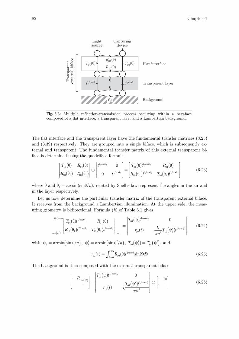
82 Chapter 6
Background
Flat interfaceT01(θ)R01(θ)
R10(θ)
Transparent layert1/cosθ t1/cosθ0
0
T10(θ)
Lightsource
Capturingdevice
Tra
nsp
aren
t ex
tern
al b
ifac
e
ρB
Fig. 6.3: Multiple reflection-transmission process occurring within a hexaface composed of a flat interface, a transparent layer and a Lambertian background.
The flat interface and the transparent layer have the fundamental transfer matrices (3.25) and (3.39) respectively. They are grouped into a single biface, which is subsequently ex-ternal and transparent. The fundamental transfer matrix of this external transparent bi-face is determined using the quadriface formula
( ) ( )
( ) ( )
( ) ( )
( ) ( )
1 1
1 1 1
1/cos 1/cos01 01 01 01
1/cos 2/cos 1/cos10 1 10 1 10 1 10 1
0
0
T R t T t R
R T t R t T t
θ θ
θ θ θ
⎡ ⎤ ⎡ ⎤⎡ ⎤θ θ θ θ⎢ ⎥ ⎢ ⎥⎢ ⎥ =⎢ ⎥ ⎢ ⎥⎢ ⎥θ θ ⎢ ⎥ ⎢ ⎥θ θ⎢ ⎥⎣ ⎦ ⎣ ⎦ ⎣ ⎦ (6.23)
where θ and θ1 = arcsin(sinθ/n), related by Snell’s law, represent the angles in the air and in the layer respectively.
Let us now determine the particular transfer matrix of the transparent external biface. It receives from the background a Lambertian illumination. At the upper side, the meas-uring geometry is bidirectional. Formula (h) of Table 6.1 gives
( )
( )( ) ( )
( ) ( )
( )
( ) ( )
11
1 1 1
1/cos1/cos01
01 01
2/cos 1/cos 1/cos10 1 10 1 10 10 12
0
dir
rad L
T tT t R
R t T t r t T tn
ψψ → θ
θ θ ′ψ
′ψ ← ←
⎡ ⎤ψ⎡ ⎤θ θ ⎢ ⎥⎢ ⎥ ⎢ ⎥=⎢ ⎥ ξ⎢ ⎥⎢ ⎥ ′θ θ ψ⎢ ⎥⎣ ⎦ π⎣ ⎦
(6.24)
with ( )1 arcsin sin /nψ = ψ , ( )1 arcsin sin /n′ ′ψ = ψ , ( ) ( )10 1 01T T′ ′ψ = ψ , and
( ) ( )
/22/cos
10 100
sin2r t R t dπ
θ
θ== θ θ θ∫ (6.25)
The background is then composed with the external transparent biface
( )( )
( )( )
1
1
1/cos01
1/cos01
10 2
0
Brad
T tR
T tr t
n
ψ
′ψ′ψ
⎡ ⎤ψ⎢ ⎥ ⋅ ρ⎡ ⎤⋅ ⎡ ⎤⎢ ⎥⎢ ⎥ ⎢ ⎥= ′⎢ ⎥ψ⎢ ⎥ ⋅ ⋅⎢ ⎥⋅ ⋅ ⎢ ⎥ ⎣ ⎦⎣ ⎦ ξ⎢ ⎥π⎣ ⎦
(6.26)

Reflectance and transmittance models 83
Its global reflectance Rrad(ψ′) is obtained thanks to the quadriface formula (5.24)
( )( ) ( )
( )
1 11/cos 1/cos01 01
2101
B
radB
T T tR
n r t
′ψ + ψ
′ψ
′ψ ψ ρξ= ⋅
π − ρ (6.27)
The corresponding reflectance factor ( ) ( )ˆ / refrad radR R R′ ′ψ ψ= , defined in reference to a perfect
white diffuser (reflectance Rref = ξ/π, see Eq. A.14) is
( )( ) ( )
( )
1 11/cos 1/cos
01 01
210
1ˆ1
B
radB
T T tR
n r t
′ψ + ψ
′ψ
′ψ ψ ρ= ⋅
− ρ (6.28)
Expression (6.28) is identical to that presented by Shore and Spoonhower [SS01], also derived independently by Elias & al. [EM01, Eq. (8)]. A step-by-step description of the multiple reflection-transmission process [HH04] also leads to the same expression.
Williams and Clapper considered only the special values n = 1.53, ψ = 45° and ψ′ = 0°. By arranging the terms of Eq. (6.28), we retrieve their original expression
( )
1/2
2.13 2/cos10
0
1ˆ 0.183 cos sin2wc
B
R t R t d−
πθ
θ=
⎡ ⎤⎢ ⎥= − θ θ θ θ⎢ ⎥ρ⎣ ⎦
∫ (6.29)
Shore and Spoonhower have also developed a model for a directional source and an inte-grating sphere. The corresponding global reflectance is expressed as
( )( ) ( )
( )
11/cos01 10
01101
Bsph
B
T t t tR R
r t
ψψ ρ= ψ +
− ρ (6.30)
A similar expression is presented in [HH04], but since the external reflection is assumed to be eliminated from the measurement, the term R10(ψ) corresponding to the specular re-flection at the air-layer interface is omitted.
Let us retrieve expression (6.30) with our compositional formalism. The particular transfer matrix of the transparent external biface is derived from Formula (g) of Table 6.1
( )( ) ( )
( ) ( )
( ) ( )
( ) ( )
1 1
1 1
1/cos 1/cos01 01 01 01
2/cos 1/cos10 1010 1 10 1
dir
sph L
T t R T t R
r t t tR t T t
ψ → θ ψ
θ θ
← ←
⎡ ⎤ ⎡ ⎤θ θ ψ ψ⎢ ⎥ ⎢ ⎥=⎢ ⎥ ⎢ ⎥⎢ ⎥θ θ ⎢ ⎥⎣ ⎦⎣ ⎦
(6.31)
where r10(t) is given by Eq. (6.25) and
( ) ( )
/21/cos
10 100
sin2t t T t dπ
θ
θ== θ θ θ∫ , (6.32)
Expression (6.30) is then obtained by applying the quadriface formula to the composition equation
( ) ( )
( ) ( )
11/cos
01 01
10 10
Bsph T t RR
r t t t
ψ⎡ ⎤ ⋅ ρ⎡ ⎤ ψ ψ⋅ ⎡ ⎤⎢ ⎥⎢ ⎥ ⎢ ⎥= ⎢ ⎥⎢ ⎥ ⋅ ⋅⎢ ⎥⋅ ⋅ ⎢ ⎥ ⎣ ⎦⎣ ⎦ ⎣ ⎦ (6.33)

84 Chapter 6
Remark: Let us again consider that the interface is rough. Since the transparent layer has a zero reflectance, there is no multiple reflection between the rough interface and the transparent layer. The transparent layer grouped with the rough interface form a scatter-ing biface, bordered at the bottom side by the Lambertian background. The resulting multiface is regular (Sect. 5.2.1). However, the multiface would be irregular if the trans-parent layer was replaced by a scattering layer having a nonzero reflectance, or if the background was scattering only instead of being Lambertian.
6.3.3 Background and transparent layer having different refractive indices
In order to cope with an eventual difference of refractive index between the layer and the background (resp. n1 and n2), it is necessary to introduce into the model an interface between them. The background-layer interface, assumed here to be flat, causes multiple reflections with the background at the lower side, and with the layer-air interface at the upper side (Fig. 6.5). This configuration has been presented very recently by Simonot & al as an extension of the Williams-Clapper model [SHH06]. The development of this model is based on a step-by-step description of the multiple reflection-transmission proc-ess of light.
ρB Background
Transparent layert1/cosθ t1/cosθ0
0
Flat interfaceT01(θ)R01(θ)
R10(θ)T10(θ)
R12(θ)Flat interfaceT12(θ)
R21(θ)T21(θ)
Lightsource
Capturingdevice
Tra
nsp
aren
t ex
tern
al b
ifac
e
Fig. 6.5: Multiple reflection-transmission process occurring within a multiface composed of a transparent layer bounded by two interfaces and a Lambertian background.
Here, the external biface is composed of the air-layer interface, the transparent layer and the layer-background interface. The fundamental transfer matrix of such a transpar-
Reflectance and transmittance models 85
ent multiface has already been developed in Sect. 6.2.1 and is given by Eq. (6.11). Ex-cepted this new fundamental transfer matrix, we have the same configuration as for the interface alone and for the transparent layer bounded by one interface.
For a bidirectional measuring geometry (incidence angle ψ and observation angle ψ′ ≠ ψ), the particular transfer matrix of the transparent external biface is (Table 6.1, formula h)
( )
( ) ( ) ( )
( ) ( )
( )
( ) ( )
012012 012
210 210 2210 1 210 1 22
0
dir
rad L
TT R
r t TR Tn
ψ →
′ψ ← ←
⎡ ⎤ψ⎡ ⎤θ θ ⎢ ⎥⎢ ⎥ ⎢ ⎥= ξ⎢ ⎥ ⎢ ⎥′ψθ θ⎢ ⎥ ⎢ ⎥⎣ ⎦ π⎢ ⎥⎣ ⎦
(6.34)
with
( ) ( )
/2
210 2100
sin2r t R dπ
θ== θ θ θ∫ , (6.35)
( )210 2T ′ψ may be replaced by ( )012T ′ψ [Eq. (3.58)]. The composition equation is
( )( )
( )( )
012
012210 2
0
Brad
TR
Tr t
n
′ψ
⎡ ⎤ψ ⋅ ρ⎢ ⎥⎡ ⎤⋅ ⎡ ⎤⎢ ⎥⎢ ⎥ ⎢ ⎥= ′ψ⎢ ⎥⎢ ⎥ ⋅ ⋅⎢ ⎥⋅ ⋅ ⎣ ⎦ξ⎢ ⎥⎣ ⎦⎢ ⎥π⎣ ⎦
(6.36)
The quadriface formula then gives the following expression for the reflectance of the back-ground coated with the transparent layer of different refractive index
( )( ) ( )
( )
012 012
22 2101
B
radB
T TR
n r t′ψ
′ψ ψ ρξ= ⋅
π − ρ (6.37)
The corresponding reflectance factor ( ) ( )ˆ / refrad radR R R′ ′ψ ψ= , defined in reference to a perfect
white diffuser (reflectance Rref = ξ/π), is
( )( ) ( )
( )
012 012
22 210
1ˆ1
B
radB
T TR
n r t′ψ
′ψ ψ ρ= ⋅
− ρ (6.38)
For an integrating sphere geometry, the transfer matrix of the transparent external biface is given by formula (g) of Table 6.1
( ) ( ) ( )
( ) ( )
( ) ( )
( ) ( )
012 012 012 012
210 210210 1 210 1
dir
sph L
T R T R
r t t tR T
ψ →
← ←
⎡ ⎤ ⎡ ⎤θ θ ψ ψ⎢ ⎥ ⎢ ⎥=⎢ ⎥ ⎢ ⎥θ θ⎢ ⎥ ⎢ ⎥⎣ ⎦⎣ ⎦ (6.39)
where ( )210r t is given by Eq. (6.35) and
( ) ( )
/2
210 2100
sin2t t T dπ
θ== θ θ θ∫ . (6.40)
The reflectance of the coated background observed with an integrating sphere is
( )( ) ( )
( )
012 012012
2101B
sphB
T t tR R
r t
ψ ρ= ψ +
− ρ (6.41)

86 Chapter 6
Note that in [SHH06], the external reflection component ( )012R ψ is omitted, being as-sumed to be discarded from the measurement.
The model of Simonot & al. is not restricted to a single transparent layer. The Lam-bertian background may be superposed with several transparent layers of different refrac-tive indices, separated by flat interfaces. The grouping of the layers and interfaces is per-formed iteratively, with a formula equivalent to the compositional formula (5.33). Once the new fundamental transfer matrix is obtained, the same development as above may be followed.
Remark: The multiface becomes irregular if either one of the interfaces is rough, or the transparent layer is replaced by a scattering layer, or the background is weakly scattering instead of being Lambertian.
Summary
We have established how, given a multiface and a measuring geometry, the reflectance and the transmittance of each face can be determined. The elaboration of reflectance and transmittance models have been illustrated with classical models, i.e. the Kubelka’s model and the Williams-Clapper model. The recent extensions of the Williams-Clapper model for the integrating sphere geometry (Shore and Spoonhower [SHO00]), and a non neglect-ible background-coating interface (Simonot, Hébert and Hersch [SHH06]) have also been retrieved.
We have not considered yet multifaces with alternations of transparent and Lamber-tian bifaces. We have neither found in the specialized literature any compositional model considering such multifaces. This is probably due to the fact that the description of a multiple reflection-transmission process in three or more superposed bifaces of different nature is hardly realizable with a step-by-step method. With the compositional model, we are now capable of considering mixed multifaces, such as superposed paper sheets (Chap-ter 7) and prints (Chapter 8). The superposition of glossy paper sheets, for example, yields a multiface comprising seven bifaces: two paper layers (Lambertian), four flat inter-faces (transparent) and the air layer between the paper sheets (obviously also transpar-ent).

87
Chapter 7.
Compositional models for paper
The present chapter aims at characterizing high quality paper sheets. The paper layer, assumed to be Lambertian, is characterized by its “intrinsic” reflectance and transmittance. It is bounded at both its sides by interfaces, assumed to be flat, char-acterized by Fresnel coefficients. A straightforward application of the compositional model gives global reflectances and transmittances of the paper sheet for a selected measuring geometry. Biface splittings enable dissociating the geometry-dependent terms from the other ones. We thus define a sheet “internal reflectance and transmit-tance” remaining invariant whatever the measuring geometry (Sect. 7.1). The rela-tionship between our compositional model and the Kubelka-Munk model is analyzed. A method for deducing the intrinsic parameters of paper from measurements is also proposed. In Sect. 7.2, an advanced model considers the superposition of two sheets with full optical contact or without contact. We use this double sheet model for de-ducing from measurements the intrinsic parameters of paper independently of the measuring geometry (Sect. 7.3).
7.1 Single paper sheet model
Papers depend on the nature of the fibers (natural or synthetic) forming the paper bulk, the chemical treatment, the addition of optical brighteners for improving the paper whiteness and the surface coating. Paper sheets are generally characterized by reflec-tances, brightness, opacity, gloss, and Kubelka-Munk coefficients [BLMC01, Nis98].
Here, paper sheets are characterized by the intrinsic reflectance and transmittance of the paper substrate layer, considered without interfaces. This requires modeling the mul-tiple reflections occurring at the internal side of the paper-air interfaces. Because of the angular dependence of the Fresnel coefficients, the measuring geometries must be taken into account. However, they may be not exactly known, e.g. when the illuminating light source is not collimated or not Lambertian as expected in our model. The observation geometry of measuring devices may also be uncertain. We therefore intent to develop a model independent of the measuring geometry.
The model presented here concerns high quality paper sheets, whose paper layer is made of a homogenous and nonfluorescent scattering layer assimilated to a Lambertian biface. White opaque plastic sheets are also concerned provided that the pigmented plas-tic scatters light sufficiently for being considered as a Lambertian layer. The surfaces of the sheet are assumed to be flat, hence forming two flat paper-air interfaces.
At the upper side of the sheet, a directional light incomes at angle ψ, and a radiance detector captures light at angle ′ψ (we note ξ′ its apparatus constant, defined in Appen-dix A.2). At the bottom side are placed a Lambertian light source and a radiance detector (apparatus constant ξ′′, observation angle ′′ψ ). For such a measuring geometry, the

88 Chapter 7
global transfer matrix of the paper sheet is termed
1 1
1 1
U U
V V
T R
R T
⎡ ⎤⎢ ⎥⎢ ⎥⎢ ⎥⎣ ⎦
(7.1)
We propose to determine the elements of this global transfer matrix according to our compositional model.
7.1.1 Global reflectance and transmittance of a paper sheet
The paper sheet is represented by a hexaface, whose bifaces are respectively the upper air-paper interface, the paper layer, and the lower air-paper interface (Fig. 7.1). Such a hexaface is regular since it does not comprise any scattering biface (Sect. 5.2.1).
Lambertiansource
Flat interface
Flat interface
Directionalsource (ψ)
Radiancedetector (ψ')
Radiancedetector (ψ'')
T01(θ)
T01(θ)R10(θ)
R01(θ)
R01(θ)
R10(θ)
Paper layerρ
ρ'τ τ
T10(θ)
T10(θ)
Fig. 7.1: Hexaface representing a paper sheet.
The Lambertian paper layer is characterized by its invariant transfer matrix (Sect. 6.1.2), containing its upper intrinsic reflectance ρ, its lower intrinsic reflectance ρ′ (generally dif-ferent from ρ) and its intrinsic transmittance τ (identical at the upper and the lower sides)
τ ρ⎡ ⎤
⎢ ⎥⎢ ⎥′ρ τ⎢ ⎥⎣ ⎦
(7.2)
The interfaces are characterized by their fundamental transfer matrix [Eq. (3.25)] whose elements are Fresnel reflection and transmission coefficients parameterized by the refrac-

Compositional models for paper 89
tive index n of the paper. Since they are external bifaces, their particular transfer matrix depends on the measuring geometry.
Let us first consider the upper interface. It is illuminated on its upper side by the di-rectional light source (incident angle ψ) and on its lower side by the Lambertian light coming from the paper layer. It is observed at the upper side by a radiance detector (ob-servation angle ψ′). With formula (h) of Table 6.1, and using relation ( ) ( )10 1 01T T′ ′ψ = ψ , the upper interface has the particular transfer matrix
( )
( ) ( ) ( )
( ) ( )
( )
( )
0101 01
10 10 10 012
0dir
rad L
TT R
R T r Tn
ψ →
′ψ ← ←
⎡ ⎤ψ⎡ ⎤θ θ ⎢ ⎥⎢ ⎥ ⎢ ⎥= ′⎢ ⎥ ξ⎢ ⎥θ θ ′ψ⎢ ⎥ ⎢ ⎥⎣ ⎦ π⎣ ⎦
(7.3)
The lower interface is illuminated by Lambertian irradiances on both its faces. Its lower face is observed by a radiance detector at angle ψ′′. Its particular transfer matrix is given by Formula (j) of Table 6.1, with reversed notations since we are in presence of a lower external biface
( ) ( )
( ) ( )
( ) ( )
( )
01 10210 10
01 0101 01
L rad
L
T rT R nR T
R t
′′→ → ψ
←
⎡ ⎤′′ξ ′′⎢ ⎥ψ⎡ ⎤θ θ ⎢ ⎥π⎢ ⎥ = ⎢ ⎥⎢ ⎥ ′′⎢ ⎥θ θ ξ⎢ ⎥ ′′⎣ ⎦ ⎢ ⎥ψ⎢ ⎥π⎣ ⎦
(7.4)
The composition equation representing the paper sheet is
( )
( )
( )
( )
01 01 1021 1
1 1 10 01201 01
0
U U
V V
T T rT R nR T r T R tn
⎡ ⎤′′ξ⎡ ⎤ψ ′′⎢ ⎥ψτ ρ⎡ ⎤ ⎡ ⎤⎢ ⎥ ⎢ ⎥π⎢ ⎥ ⎢ ⎥⎢ ⎥= ⎢ ⎥′ξ⎢ ⎥ ⎢ ⎥⎢ ⎥ ′ρ τ ′′⎢ ⎥ξ′ψ ⎢ ⎥⎢ ⎥ ⎢ ⎥ ⎣ ⎦⎣ ⎦ ′′⎢ ⎥ψπ⎣ ⎦ ⎢ ⎥π⎣ ⎦
(7.5)
The hexaface formula (5.27) applied to the composition equation (7.5) gives the expres-sion for the global transfer matrix of the paper sheet
( ) ( ) ( ) ( ) ( )
( ) ( ) ( ) ( )
21001 01 01 01
2 21 1
21 1 1001 01 01 01 01
2 2
U U
V V
rT T T TT R n D n DR T rR t T t T
n D n D
⎡ ⎤′ρ − ρρ − τ′′ ′′ ′ ′ξ ψ ψ ξ ψ ψτ⎢ ⎥⋅ ⋅⎡ ⎤ ⎢ ⎥′ ′π π⎢ ⎥ ⎢ ⎥=⎢ ⎥ ⎢ ⎥′ ′ρ − ρρ − τ′′ ′′ ′′ ′′ ′ ′⎢ ⎥ ξ ψ ξ ψ ξ ψ τ⎢ ⎥⎣ ⎦ + ⋅ ⋅⎢ ⎥⎢ ′ ′ ⎥π π π⎣ ⎦
(7.6)
with ( )( ) 210 10 101 1D r r r′ ′ ′= − ρ − ρ − ττ .
In the case of a symmetric paper sheet, both faces of the paper layer have the same intrinsic reflectance (ρ = ρ′). The global transfer matrix of the sheet becomes
( ) ( ) ( ) ( ) ( )
( ) ( ) ( ) ( )
2 21001 01 01 01
2 21 1
2 21 1 1001 01 01 01 01
2 2
U U
V V
rT T T TT R n D n DR T rR t T t T
n D n D
⎡ ⎤ρ − ρ − τ′′ ′′ ′ ′ξ ψ ψ ξ ψ ψτ⎢ ⎥⋅ ⋅⎡ ⎤ ⎢ ⎥′ ′π π⎢ ⎥ ⎢ ⎥=⎢ ⎥ ⎢ ⎥ρ − ρ − τ′′ ′′ ′′ ′′ ′ ′⎢ ⎥ ξ ψ ξ ψ ξ ψ τ⎢ ⎥⎣ ⎦ + ⋅ ⋅⎢ ⎥⎢ ′ ′ ⎥π π π⎣ ⎦
(7.7)
with ( ) ( )2 210 101D r r′ = − ρ − τ .

90 Chapter 7
7.1.2 Internal reflectance and transmittance of a paper sheet
Eq. (7.6) shows clearly that the sheet global transfer matrix depend on the measuring geometry. However, this dependence is only due to the external reflectance, the penetra-tion transmittance and the exit transmittance of the interfaces. In order to dissociate the geometry-dependent terms from the other terms, we propose to split the bifaces represent-ing the interfaces (see Sect. 5.4). Their transfer matrix, given by Eqs. (7.3) and (7.4), are thus represented by a composition of two transfer matrices, a first one containing the external reflectance, the penetration transmittance and the exit transmittance (geometry-dependent terms), the second one containing the internal reflectance which is geometry-independent. The upper biface is split as
( )
( )
( )
( )
01 01
1010 01 012 2
0 0 1 0
10
T T
rr T Tn n
⎡ ⎤ ⎡ ⎤ψ ψ ⎡ ⎤⎢ ⎥ ⎢ ⎥ ⎢ ⎥⎢ ⎥ ⎢ ⎥=′ ′ξ ξ ⎢ ⎥⎢ ⎥ ⎢ ⎥′ ′ψ ψ ⎢ ⎥⎢ ⎥ ⎢ ⎥ ⎣ ⎦π π⎣ ⎦ ⎣ ⎦
(7.8)
and the lower biface is split as
( )
( )
( )
( )
01 10 012 210
01 01 01 01
01
0 1
T r Trn n
R t R t
⎡ ⎤ ⎡ ⎤′′ ′′ξ ξ′′ ′′⎢ ⎥ ⎢ ⎥ψ ψ⎡ ⎤⎢ ⎥ ⎢ ⎥π π⎢ ⎥=⎢ ⎥ ⎢ ⎥⎢ ⎥′′ ′′⎢ ⎥ ⎢ ⎥ξ ξ⎢ ⎥⎣ ⎦′′ ′′⎢ ⎥ ⎢ ⎥ψ ψ⎢ ⎥ ⎢ ⎥π π⎣ ⎦ ⎣ ⎦
(7.9)
Bounded paper layer
Lambertiansource
Directionalsource (ψ)
Radiancedetector (ψ')
Radiancedetector (ψ'')
T01(θ)
T10(θ)
T10(θ)
T01(θ)0
R01(θ)
R01(θ)
0
R1
R′1
T1 T1
1 10
R10(θ)
ρ
ρ′τ τ
1 1R10(θ)
0
T10(θ) T01(θ)0
R01(θ)
T10(θ) T01(θ)R10(θ)
0
Paper layer
Flat interface
Flat interface
Fig. 7.2: Representation of a paper sheet with split interfaces. The paper layer and its bordering interfaces form a geometry-independent biface, called “bounded paper layer”.

Compositional models for paper 91
The composition equation of the paper sheet, originally given by Eq. (7.5), becomes
( )
( )
( )
( )
01 0121 1 10
101 1 01201 01
0 01 0 1
1 0 10
U U
V V
T TT R r nrR T T R tn
⎡ ⎤′′ξ⎡ ⎤ψ ′′⎢ ⎥ψ⎡ ⎤ ⎡ ⎤ τ ρ ⎡ ⎤⎢ ⎥ ⎡ ⎤ ⎢ ⎥π⎢ ⎥ ⎢ ⎥ ⎢ ⎥⎢ ⎥ ⎢ ⎥= ⎢ ⎥′ξ⎢ ⎥ ⎢ ⎥ ⎢ ⎥ρ τ⎢ ⎥ ⎢ ⎥ ′′⎢ ⎥ξ′ψ ⎣ ⎦⎢ ⎥ ⎢ ⎥ ⎢ ⎥⎢ ⎥ ⎣ ⎦ ⎣ ⎦⎣ ⎦ ′′⎢ ⎥ψπ⎣ ⎦ ⎢ ⎥π⎣ ⎦
(7.10)
As indicated in Fig. 7.2, the three central bifaces are regrouped into a single biface, called the “bounded paper layer”. The composition of the three central transfer matrices in Eq. (7.10), calculated according to the hexaface formula (5.27), gives the internal transfer matrix of the paper sheet
( )
( )
21 1 10 10
2101 1 10
1 0 1 1
1 0 1
T R r r
rR T D r
⎡ ⎤τ ρ ′⎡ ⎤ ⎡ ⎤ ⎡ ⎤ τ ρ − ρρ − τ⎡ ⎤ ⎢ ⎥⎢ ⎥ ⎢ ⎥ ⎢ ⎥⎢ ⎥= = ⎢ ⎥⎢ ⎥ ⎢ ⎥ ⎢ ⎥⎢ ⎥′ρ τ′ ′ ′ ⎢ ⎥′ ′ρ − ρρ − τ τ⎢ ⎥ ⎢ ⎥⎢ ⎥ ⎢ ⎥⎣ ⎦⎣ ⎦ ⎣ ⎦⎣ ⎦ ⎣ ⎦
(7.11)
where ( )( ) ( )210 10 101 1D r r r′ ′= − ρ − ρ − τ .
Reflectances R1 and 1R′ are called the internal reflectances of the paper sheet and transmittances T1 and 1T ′ are called the internal transmittances. They take into account the internal reflections at the paper-air interfaces, but not the surface reflection, the pene-tration nor the exit. Eq. (7.11) puts into evidence the fact that internal transmittances T1 and 1T ′ are equal, even though the paper sheet is not symmetric. Light therefore crosses the bounded paper layer with the same attenuation independently on the sense of cross-ing. This property1 may be given the name of “principle of nonpolarity of internal trans-mittance”, in reference to the “principle of nonpolarity of transmittance” formulated by Kubelka for Lambertian multifaces having all the same refractive index (Sect. 6.2.2).
The relationship between the global and the internal transfer matrices follows directly Eq. (7.10)
( )
( )
( )
( )
0101
21 11 1
011 1 1 1 01201
0 0
0
U U
V V
TT T RT R nTR T R T R
tn
⎡ ⎤′′ψ⎡ ⎤ψ ⎢ ⎥′′ξ⎡ ⎤⎡ ⎤ ⎢ ⎥ ⎢ ⎥π⎢ ⎥⎢ ⎥ ⎢ ⎥ ⎢ ⎥= ′ ⎢ ⎥⎢ ⎥ ψ⎢ ⎥ ⎢ ⎥′ ′′ψ′ ⎢ ⎥ξ⎢ ⎥ ⎢ ⎥⎣ ⎦ ⎢ ⎥⎣ ⎦ ′′ξ⎢ ⎥π⎣ ⎦ ⎢ ⎥π⎣ ⎦
(7.12)
Eq. (7.12) characterizes the dissociation in our single sheet model of the geometry-dependent and the geometry-independent terms. It tells us, in particular, that the global transmittances TU1 and TV1 are different only due to the light penetration and exit across the interfaces.
In the case of a symmetric paper sheet (ρ = ρ′), both internal reflectances are also equal, i.e. R1 = 1R′ . Eq. (7.11) becomes
( ) ( )
( )( )
2 21 1 10
2 2 2 21 1 10 10 10
1
1
T R r
R T r r r
⎡ ⎤⎡ ⎤ τ ρ − ρ − τ⎢ ⎥⎢ ⎥ = ⎢ ⎥⎢ ⎥ ⎢ ⎥− ρ − τ ρ − ρ − τ τ⎢ ⎥⎣ ⎦ ⎣ ⎦
(7.13)
⎯⎯⎯⎯⎯⎯⎯⎯⎯⎯⎯ 1 The non-polarity of the bounded paper layer is also valid when the interfaces have different pro-perties (relative refractive index, roughness, etc.)

92 Chapter 7
7.1.3 Relation with the Kubelka-Munk model
We have characterized with expression (7.6) the optical properties of a paper sheet as functions of the intrinsic reflectances ρ and ρ′ and transmittance τ of the paper layer. However, the characterization of paper is traditionally expressed with the parameters of the Kubelka-Munk model [KM31], i.e. with a scattering coefficient S, an absorption coeffi-cient K, and the layer thickness h [BLMC01]. Let us establish the connection between the two models [HH06].
First note that the Kubelka-Munk model can be used only if the paper layer has the same coefficients at every point. We must therefore consider in our single sheet model that the paper layer has identical faces, i.e. ρ = ρ′.
We can choose among two methods for obtaining the global reflectance and transmit-tance of the sheet as functions of the Kubelka-Munk parameters. In the first method, which may be called the “direct method”, the reflections and the transmissions by the interfaces are taken into account as boundary conditions while solving the Kubelka-Munk differential equation system. This corresponds exactly to the configuration of a Lamber-tian layer bounded by two bifaces, presented in Sect. 4.3.5. Here, the two bifaces are the flat interfaces. The global reflectance and transmittance of the sheet have the same ex-pressions as Rb and Tb [Eqs. (3.105) and (3.106)], with the specific elements
( )
( )01
0110 2
0u u
u u
Tp sTr x r
n
⎡ ⎤ψ⎢ ⎥⎡ ⎤ ⎢ ⎥⎢ ⎥ = ′ψ⎢ ⎥⎢ ⎥ ξ⎣ ⎦ ⎢ ⎥⎢ ⎥π⎣ ⎦
and
( )
( )
01102
0101
v v
v v
Trx r n
s p Rt
⎡ ⎤′′ψ⎢ ⎥ξ⎡ ⎤ ⎢ ⎥π⎢ ⎥ ⎢ ⎥=⎢ ⎥ ⎢ ⎥′′ψ⎣ ⎦ ⎢ ⎥ξ⎢ ⎥π⎣ ⎦
(7.14)
The second method, which may be called the “two steps method”, consists in solving the Kubelka-Munk system for the Lambertian layer alone without considering the interfaces, which yields expressions (3.96) and (3.97) for its intrinsic reflectance ρ and transmittance τ, and then in using the compositional model (Eqs. (7.5) and (7.6)) for taking into ac-count the reflections and the transmissions at the interfaces. One may verify that both methods are equivalent. The second method may be considered as an extended Saunder-son correction for two bounding interfaces.
7.1.4 Deducing intrinsic parameters of paper from measurements
We would like to determine the intrinsic parameters ρ and ρ′ and τ of a nonsymmetric paper sheet. We use a bidirectional spectrophotometer (typically build on the 45°/0° ge-ometry) either in reflectance mode (light source on) or in transmittance mode (light source off). The spectrophotometer is placed upon the paper sheet, and a diffusing light table, placed below, is used as light source in transmittance mode. The measuring geome-try is thus similar to the measuring geometry considered in Sect. 7.1.2, except that there is no detector at the lower side.
The spectrophotometer is first used in reflectance mode. We measure the reflectance Rref of a perfect white diffuser, given by Eq. (A.14)
/refR ′= ξ π (7.15)

Compositional models for paper 93
Then, we measure the upper global reflectance RU1 of the sheet as weel as the upper global reflectance 1UR of the same sheet positioned upside-down. According to Eq. (7.6), our model expresses reflectance RU1 as
( ) ( )( )
( )( ) ( )
210
1 01 01 2210 10 101 1
U
rR T T
n r r r
′ρ − ρρ − τ′ξ ′= ψ ψπ ′− ρ − ρ − τ
, (7.16)
Reflectance 1UR is similarly expressed, the intrinsic reflectances ρ and ρ’ being replaced by each other
( ) ( )( )
( )( ) ( )
210
1 01 01 2210 10 101 1
U
rR T T
n r r r
′ ′ρ − ρρ − τ′ξ ′= ψ ψπ ′− ρ − ρ − τ
(7.17)
The spectrophotometer is then used in transmittance mode. A first transmittance Tref is measured without the sheet, considering air as the reference transmitter. In a similar manner as the perfect white diffuser, the light table emits a Lambertian irradiance, yield-ing a transmittance of air
/refT ′= ξ π (7.18)
The lower transmittance TV1 of the sheet is given by Eq. (7.6)
( ) 1 01 012VT t Tn D
′ξ τ′= ψ′π (7.19)
In order to have expressions independent of the apparatus constant ξ′, we rather consider the reflectance factors 1 1U U refR R R= and 1 1U U refR R R= and the transmittance factor
1 1ˆ /V V refT T T= . We obtain the three following equations
( ) ( )( )
( )( ) ( )
210
1 01 01 2210 10 10
1ˆ1 1
U
rR T T
n r r r
′ρ − ρρ − τ′= ψ ψ
′− ρ − ρ − τ (7.20)
( ) ( )( )
( )( ) ( )
210
1 01 01 2210 10 10
1ˆ1 1
U
rR T T
n r r r
′ ′ρ − ρρ − τ′= ψ ψ
′− ρ − ρ − τ (7.21)
and
( )( )( ) ( )
1 01 01 2210 10 10
1ˆ1 1
VT t Tn r r r
τ′= ψ′− ρ − ρ − τ
(7.22)
Knowing the refractive index of the paper, the Fresnel coefficients and their integrations over the hemisphere (r10 and t01, see Sect. 3.2.2) can be computed. The three equations (7.20), (7.21) and (7.22) thus allow to deduce wavelength by wavelength the intrinsic parameters ρ, ρ′ and τ.
The principal drawback of this method is the fact that it depends on the measuring geometry, due to the presence of the terms T01(ψ), T01(ψ′) and t01. Although these terms are easily computable thanks to Fresnel formulae [Eqs. (3.20), (3.22) and (3.28)], we are not always certain that the conditions of illumination respect our assumptions. We would

94 Chapter 7
like to have three equations completely independent of the measuring geometry. The dou-ble sheet model that we present now makes it possible.
7.2 The double sheet model
As shown in Sect. 7.1.2, a single paper sheet may be characterized by an internal transfer matrix whose internal reflectances and transmittances R1, 1R′ and T1 are inde-pendent of the measuring geometry. The geometry-dependent terms, i.e. the surface re-flectances s, the penetration transmittances p and the exit transmittances x of the inter-faces, are placed in separate transfer matrices. For the selected measuring geometry, the relation between the global and the internal transfer matrices is
1 1 1 11 1
1 1 1 1 1 1
0 0
u u u v u u uU U v
u v vV V v v v v u
p s T R p x T s p x RT R x
x s pR T R T s p x R p x T
⎡ ⎤ ⎡ ⎤+⎡ ⎤ ⎡ ⎤ ⎡ ⎤⎢ ⎥ ⎢ ⎥⎢ ⎥ ⎢ ⎥ ⎢ ⎥= =⎢ ⎥ ⎢ ⎥⎢ ⎥ ⎢ ⎥ ⎢ ⎥′ ′+⎢ ⎥ ⎢ ⎥⎢ ⎥ ⎣ ⎦ ⎣ ⎦⎣ ⎦ ⎣ ⎦ ⎣ ⎦ (7.23)
Let us now superpose two identical paper sheets, the lower sheet being positioned upside-down. Thus, the resulting double sheet is symmetric. Selecting the same measuring ge-ometry as for a single sheet, we have an equivalent relation between the global transfer matrix of the double sheet and its internal transfer matrix
2 2 2 2 2 2
2 2 2 2 2 2
0 0
u uU U u v u u uv
u v vV V v v v v u
p sT R T R p x T s p x Rx
x s pR T R T s p x R p x T
⎡ ⎤ ⎡ ⎤ ⎡ ⎤+⎡ ⎤ ⎡ ⎤⎢ ⎥ ⎢ ⎥ ⎢ ⎥⎢ ⎥ ⎢ ⎥= =⎢ ⎥ ⎢ ⎥ ⎢ ⎥⎢ ⎥ ⎢ ⎥ +⎢ ⎥ ⎢ ⎥ ⎢ ⎥⎣ ⎦ ⎣ ⎦⎣ ⎦ ⎣ ⎦ ⎣ ⎦ (7.24)
In Eq. (7.24), the upper and lower internal reflectances (R2) are identical due to the sym-metry of the double sheet.
It may be observed from Eqs. (7.23) and (7.24) that the ratio of global transmittances TV2/TV1 is equal to the ratio of internal transmittances T2/T1
2 2 2
1 1 1
V v u
V v u
T p x T TT p x T T
= = (7.25)
Since both internal transmittances T1 and T2 are geometry-independent, the ratio TV2/TV1 is also geometry-independent.
In the case of the reflectance, the ratio of measured reflectances RU2/RU1 (likewise the ratio 2 1/U UR R ) is geometry-independent only when the surface reflection is discarded from the measure (su = 0), which is the case when a 45°/0° geometry is used
2 2 2
1 1 1
U u u
U u u
R p x R RR p x R R
= = and 2 2 2
1 1 1
u u
U u u
R p x R RR p x R R
= =′ ′
(7.26)
Let us develop expressions for R2 and T2 as functions of the paper intrinsic parameters ρ, ρ′ and τ. This will then allow deducing these parameters from the geometry independ-ent equations (7.25) and (7.26).

Compositional models for paper 95
7.2.1 Model for a full contact between the sheets
When the two identical sheets are in full optical contact, there is not interface between the paper layers, which thus form a double layer of paper. The external interfaces are split in the same manner as for a single sheet (Sect. 7.1.2). We may therefore represent the double sheet by the composition equation
2 2 10
102 2
1 0 1 0 0 1 0 1
u uU U v
u v vV V
p sT R r x
x s prR T
τ ρ⎡ ⎤ ⎡ ⎤ ⎡ ⎤⎡ ⎤ ⎡ ⎤′⎡ ⎤ ⎡ ⎤τ ρ⎢ ⎥ ⎢ ⎥ ⎢ ⎥⎢ ⎥ ⎢ ⎥⎢ ⎥ ⎢ ⎥=⎢ ⎥ ⎢ ⎥ ⎢ ⎥⎢ ⎥ ⎢ ⎥⎢ ⎥ ⎢ ⎥′ρ τ ρ τ⎢ ⎥ ⎢ ⎥⎢ ⎥ ⎢ ⎥ ⎢ ⎥⎣ ⎦ ⎣ ⎦⎣ ⎦ ⎣ ⎦⎣ ⎦ ⎣ ⎦⎣ ⎦ (7.27)
The internal transfer matrix of the double sheet results from the composition of the four central transfer matrices. The quadriface formula (5.24) is first applied to the two transfer matrices of the paper layers
2 2
2 22 2 10
2 2102 2
2 2
1 0 11 1
1 0 1
1 1
T R r
rR T
⎡ ⎤′τ τ ρ⎢ ⎥ρ +⎡ ⎤ ⎡ ⎤ ⎡ ⎤⎢ ⎥′ ′− ρ − ρ⎢ ⎥ ⎢ ⎥ ⎢ ⎥⎢ ⎥=⎢ ⎥ ⎢ ⎥ ⎢ ⎥⎢ ⎥′τ ρ τ⎢ ⎥ ⎢ ⎥ ⎢ ⎥⎢ ⎥⎣ ⎦ ⎣ ⎦⎣ ⎦ ρ +⎢ ⎥′ ′− ρ − ρ⎣ ⎦
(7.28)
Then, the hexaface formula (5.27) is applied to Eq. (7.28). As a result, the internal reflec-tance R2 and transmittance T2 of the double sheet are
2 2 2
2 102
11 1 1
R rD
⎡ ⎤⎛ ⎞⎛ ⎞′ρ τ τ τ⎟ ⎟⎜ ⎜⎢ ⎥⎟ ⎟= ρ + − ρ + ρ +⎜ ⎜⎟ ⎟⎢ ⎥⎜ ⎜⎟ ⎟⎜ ⎜′ ′ ′− ρ − ρ + ρ⎝ ⎠⎝ ⎠⎣ ⎦ and
2
2 2
11
TD
τ= ⋅
′− ρ (7.29)
with 2 22 2
10 10 102 211 1
D r r r⎛ ⎞ ⎛ ⎞′ρ τ τ⎟ ⎟⎜ ⎜⎟ ⎟= − ρ − +⎜ ⎜⎟ ⎟⎜ ⎜⎟ ⎟⎜ ⎜′ ′− ρ − ρ⎝ ⎠ ⎝ ⎠
(7.30)
The assumption of full optical contact between paper sheets is an ideal condition that is rarely realizable in practice, because bubbles or thin layers of air may have a nonneglect-ible effect. Instead, we separate the two sheets and thus create a planar air layer between them.
7.2.2 Model without contact between the sheets
The two paper sheets are now separated by a layer of air. The lower sheet is still iden-tical to the upper sheet but positioned upside-down. The resulting multiface is composed of seven bifaces: four interfaces, two paper layers and the air layer. As previously, all the flat interfaces are split. The internal reflections at the paper side of the interfaces are con-sidered together with the paper layers. We thus obtain two bounded paper layers (see Fig. 7.3) identical to those characterized in Sect. 7.1.2. Therefore, we reuse the internal reflectances R1 and 1R′ and the internal transmittance T1 given by the single sheet inter-nal transfer matrix (7.11). Because the two sheets are reversed, the upper and the lower bounded paper layers have slightly different transfer matrices, i.e. respectively
1 1
1 1
T R
R T
⎡ ⎤⎢ ⎥⎢ ⎥′⎢ ⎥⎣ ⎦
and 1 1
1 1
T R
R T
⎡ ⎤′⎢ ⎥⎢ ⎥⎢ ⎥⎣ ⎦
(7.31)

96 Chapter 7
Paper layer
Air layer
Flat interface
Flat interface
Flat interface
Flat interface
Bounded paper layer
Bounded air layer
Bounded paper layer
Paper layer
τ τρ′
ρ
R10(θ)
1 1
11
0
0
τ τ
R10(θ)
ρ
ρ′
1 10
R10(θ)
T01(θ) T10(θ)R01(θ)
0
1 10
0
T10(θ) T01(θ)0
R01(θ)
1 1R10(θ)
0
xv pv
0
sv
0
0
Lightsource
Capturingdevice
Lightsource
Capturingdevice
T1
T1
T1
T1
R′1
R1
R1
R′1
Ta Ta
Ra
Ra
0
xv pvsv
pu xu
supu xu
su
Fig. 7.3: Representation of two paper sheets superposed without contact. The air layer between the paper sheets and its bordering interfaces form a transparent multiface: the “bounded air layer”.

Compositional models for paper 97
The air layer has a zero reflectance and a unit transmittance. Its transfer matrix is
1 0
0 1
⎡ ⎤⎢ ⎥⎢ ⎥⎢ ⎥⎣ ⎦
(7.32)
We call “bounded air layer” the air layer considered with its bordering interfaces, ex-cluded the paper-side reflections which are already embodied into the bounded paper lay-ers. The fundamental transfer matrix of the bounded air layer results from the following composition
( )
( ) ( )
( ) ( )
( )1 0 010 01 01
0 0 101 01 10
0 1 0
0 1 0
T T R
R T T
⎡ ⎤ ⎡ ⎤θ θ θ⎡ ⎤⎢ ⎥ ⎢ ⎥⎢ ⎥⎢ ⎥ ⎢ ⎥⎢ ⎥θ θ θ⎢ ⎥ ⎢ ⎥⎢ ⎥⎣ ⎦⎣ ⎦ ⎣ ⎦ (7.33)
Composition (7.33) should be computed first for the two polarization components and then, by averaging, for natural light. However, a numerical evaluation shows that for a standard refractive index of paper close to 1.5, the composition can be performed directly with the Fresnel coefficients for natural light. The hexaface formula (5.27) thus gives the following fundamental transfer matrix for the bounded air layer
( ) ( )( )
( ) ( ) ( )( )
( ) ( ) ( )( )
( ) ( )( )
1 0 1 0 110 01 10 01 102 2
0 001 01
1 0 1 1 010 01 10 10 012 2
0 001 01
1 1
1 1
T T T T R
R R
T T R T T
R R
⎡ ⎤θ θ θ θ θ⎢ ⎥⎢ ⎥θ θ− −⎢ ⎥⎢ ⎥θ θ θ θ θ⎢ ⎥⎢ ⎥θ θ− −⎢ ⎥⎣ ⎦
(7.34)
Eq. (7.34) may be simplified using relations ( ) ( )0 101 10R Rθ θ= , ( ) ( )0 101 10T Tθ θ= . With relation ( ) ( )1 110 101T Rθ θ= − [Eq. (3.22)], one has
( ) ( )( ) ( )( ) ( )( ) ( )20 1 1 1 101 10 10 10 101 1 1 1R R R R Tθ θ θ θ θ− = + − = +
The bounded air layer is symmetric. Both its faces receives a Lambertian illumination. They have therefore the same reflectance Ra and the same transmittance Ta
( )( )
( ) ( )( )
( ) ( )( )
( )( )
1 1 110 10 10
1 110 10
1 1 110 10 10
1 110 10
1 1
1 1
L
a a
a a
L
T R TT R R RR T R T T
R R
→
←
⎧ ⎫⎡ ⎤⎪ ⎪θ θ θ⎪ ⎪⎢ ⎥⎪ ⎪⎪ ⎪⎡ ⎤ ⎢ ⎥θ θ+ +⎪ ⎪⎪ ⎪⎢ ⎥ ⎢ ⎥= ⎨ ⎬⎢ ⎥ ⎢ ⎥θ θ θ⎪ ⎪⎪ ⎪⎣ ⎦ ⎢ ⎥⎪ ⎪⎪ ⎪⎢ ⎥θ θ+ +⎪ ⎪⎣ ⎦⎪ ⎪⎩ ⎭
(7.35)
According to Eq. (6.2), one obtains
( ) ( )
( )
/2 110 10 11 1
0110
sin21a
R TR d
R
π
θ=
θ θ= θ θ
θ+∫ (7.36)
and
( )
( )
/2110
1 10
110
sin21a
TT d
R
π
θ=
θ= θ θ
θ+∫ (7.37)

98 Chapter 7
Remark: There is no absorption within the bounded air layer. The principle of conserva-tion of energy should therefore be satisfied. The sum of reflectance Ra and transmittance Ta yields the fraction of Lambertian light coming from the paper layer that is not inter-nally reflected by the paper-air interface, i.e. 101a aR T r+ = − .
Since their expression relies only on Fresnel coefficients, r10, Ra and Ta depend only on the refractive index n of the paper. Numerical values of these terms are proposed for re-fractive indices comprised between 1.45 and 1.55 in Table 7.1.
Table 7.1: Numerical values of r10, Ra and Ta as functions of the paper refractive index n
n 1.45 1.46 1.47 1.48 1.49 1.50 1.51 1.52 1.53 1.54 1.55
r10
Ra
Ta
0.565
0.028
0.408
0.571
0.028
0.401
0.578
0.028
0.394
0.584
0.028
0.388
0.590
0.028
0.382
0.596
0.028
0.375
0.602
0.028
0.369
0.608
0.028
0.363
0.614
0.028
0.358
0.620
0.029
0.352
0.625
0.029
0.346
The multiface representing the double sheet is reduced to five bifaces (see Fig. 7.3): the upper bounded paper layer, the bounded air layer, the lower bounded paper layer, and the two geometry-dependent external bifaces. Composing the three “bounded layers” yields the internal transfer matrix of the double sheet
1 12 2 1 1
2 2 1 1 1 1
a a
a a
T RT R T R T R
R T R TR T R T
⎡ ⎤ ⎡ ⎤′⎡ ⎤ ⎡ ⎤⎢ ⎥ ⎢ ⎥⎢ ⎥ ⎢ ⎥= ⎢ ⎥ ⎢ ⎥⎢ ⎥ ⎢ ⎥′⎢ ⎥ ⎢ ⎥⎢ ⎥ ⎢ ⎥⎣ ⎦ ⎣ ⎦⎣ ⎦ ⎣ ⎦
(7.38)
According to the hexaface formula (5.27), we obtain for the internal reflectance of the double sheet
( )
( ) ( )
2 212
2 1 1 2 2
1 11
a a a
a a
R R T RR R T
R R T R
′− −= +
′ ′− − (7.39)
and for its internal reflectance
( ) ( )
21
2 2 2
1 11a
a a
TTT
R R T R=
′ ′− − (7.40)
When the superposed sheets are symmetric, their internal reflectances R1 and 1R′ are equal [see Eq. (7.13)]. Thus, the internal reflectance and transmittance of the double sheet become
( )
( ) ( )
2 212
2 1 1 2 21 11
a a a
a a
R R T RR R T
R R T R
− −= +
− − (7.41)
and
( ) ( )
21
2 2 21 11a
a a
TTT
R R T R=
− − (7.42)

Compositional models for paper 99
7.3 Experimental results
The single and double sheet models are used in the context of a reflectance and trans-mittance model for printed sheets (see Chapter 8). Two different printing supports are used: opaque white PVC pigmented with titanium dioxide, of refractive index 1.54, and high-quality paper, of refractive index assumed to be 1.5. Both types of sheets are sym-metric (ρ = ρ′), nonfluorescent and have smooth surfaces. We want to deduce the intrin-sic reflectance ρ(λ) and transmittance τ(λ) from the spectral measurements in reflectance mode and transmittance mode. First, a geometry-dependent equations are used for deduc-ing ρ and τ. Then, in order to ascertain the modelization of the measuring geometry in transmittance mode, a geometry-independent equation provided by the noncontact double sheet model is used.
The reflectance spectrum RU1(λ) of a single sheet is measured with the portative GrategMacbethTM Eye-One spectrophotometer, based on the 45°/0° geometry (see Sect. 1.3.1). First, the spectrum of a reference white tile is measured. Then, the spectrum of the selected specimen is measured. The spectrophotometer gives directly the ratio of the specimen’s spectrum to the reference spectrum. It therefore gives a reflectance factor spectrum, noted ( )1UR λ .
( )1UR λ , given by Eq. (7.21) with ρ = ρ′, ψ = 45°, and ψ′ = 0°, is a function of the pa-per intrinsic reflectance ρ(λ) and transmittance τ(λ)
( )( ) ( ) ( )
( ) ( )
2 21001 01
1 2 2210 10
0 45ˆ1
U
rT TR
n r r
ρ − ρ − τ° °λ = ⋅
− ρ − τ (7.43)
In transmittance mode, we measure the flux Φ1(λ) transmitted through the printing sup-port and the flux Φref(λ) coming from the light table. The ratio Φ(λ)/ Φref(λ) gives the transmittance factor ( )1UT λ , expressed by Eq. (7.21) with ρ(λ) = ρ′(λ) and ψ′ = 0°
( )( )
( ) ( )01 01
1 2 2210 10
0ˆ1
V
t TT
n r r
° τλ = ⋅
− ρ − τ (7.44)
The intrinsic reflectance ρ(λ) and transmittance τ(λ) are deduced numerically from Eqs. (7.43) and (7.44). Measured transmittance factors ( )1UR λ and ( )1UT λ are plotted in Fig. 7.4a for both the white PVC and the high quality paper. The deduced spectra of ρ(λ) and τ(λ) correspond to the solid curves plotted in Fig. 7.4c.
In order to check whether the light table used for transmittance measurements is Lambertian as expected, we use the geometry-independent equations provided by the noncontact double sheet model. We measure the flux Φ2(λ) of the two face-to-face super-posed sheets. Measured fluxes Φ1(λ) (single sheet) and Φ2(λ) (double sheet) are plotted in Fig. 7.4b. The single sheet and the double sheet receives a same incident flux Φi(λ). The ratios Φ1(λ)/Φi(λ) and Φ2(λ)/Φi(λ) correspond respectively to the global transmittance of the single sheet, TV1(λ), and the global transmittance of the double sheet, TV2(λ). How-ever, in the ratio TV2(λ)/TV1(λ), the incident flux Φi(λ) cancels
( )( )
( )( )
Φ λ λ=
Φ λ λ2 2
1 1
V
V
T
T (7.45)

100 Chapter 7
According to Eq. (7.25), the ratio of global transmittances TV2(λ)/TV1(λ) is equal to the ratio of internal transmittances T2(λ)/T1(λ). From Eq. (7.42), we have
( )( )
( )
( )[ ] ( )[ ]2 1
2 21 1 11
a
a a
T TT
T R R T R
λ λ=
λ − λ − λ (7.46)
where R1(λ) and T1(λ) are given by (7.13)
( )( ) ( ) ( )
( )[ ] ( )[ ]
2 210
1 2 210 101
rR
r r
⎡ ⎤ρ λ − ρ λ − τ λ⎣ ⎦λ =− ρ λ − τ λ
and ( )( )
( )[ ] ( )[ ]1 2 210 101
Tr r
τ λλ =
− ρ λ − τ λ (7.47)
ρ(λ) and transmittance τ(λ) are again calculated, this time from the equation system formed by Eqs. (7.43) and (7.46). Eq. (7.43) is a geometry-dependent equation, where the 45°/0° geometry used in reflectance model is modeled, but we consider that this geometry is certain. However, Eq. (7.46) is geometry independent. This avoid to model the uncer-tain measuring geometry used in transmittance mode. The deduced spectra of ρ(λ) and τ(λ) are plotted with dashed lines in Fig 8.4(c). They are compared with the spectra ρ(λ) and τ(λ) previously deduced from Eqs. (7.43) and (7.44), plotted with solid lines. The small difference between the spectra obtained from the two methods for short and large wavelength is due to the low emission of the light table in these spectral ranges, which induces some noise in the measurements. The good matching of the curves in the reste of the spectrum confirms that the assumption of Lambertian illumination was satisfied. It is also a partial validation of our two superposed sheet model.
High quality paper High quality paperHigh quality paper
1
2
3
4
5
6
1
2
3
4
PVC PVCPVC
0.2
0.4
0.6
0.8
1
0.2
0.4
0.6
0.8
1
0.2
0.4
0.6
0.8
1
0.2
0.4
0.6
0.8
1
400 500 600 700 λ
400 500 600 700 λ 400 500 600 700 λ
400 500 600 700 λ 400 500 600 700 λ
400 500 600 700 λ
RU1^
dΦ1
dΦ2
ρ
τ
ρ
τ
dΦ1
dΦ2
TU1^
RU1^
TU1^
(a) (b) (c)
Fig. 7.4: (a) Reflectance factor and transmittance factor spectra measured on a single sheet; (b) measured flux spectra transmitted through (solid line:) the single and (dashed line:) the double sheets, expressed in arbitrary units; (c) intrinsic reflectance and transmittance spectra of the paper layer fitted from (solid line:) spectra plotted in a) and (dashed line:) spectra plotted in b).

Compositional models for paper 101
Summary
We have applied the compositional model to the characterization of opaque and glossy paper sheets (Lambertian paper layer and flat interfaces with air). The representation of the paper sheet by a regular hexaface and the use of the hexaface formula enables ex-pressing in a straightforward manner its global reflectance and transmittance for various measuring geometries. Furthermore, thanks to splits of the air-paper interfaces, we have dissociated the terms depending on the measuring geometry and the other terms. We thus have defined “internal” reflectances and transmittances, corresponding to the geometry-independent part of the global reflectances and transmittances. The compositional model appears to be adequate for the characterization of paper, in particular for the obtention of its intrinsic reflectances and transmittance. These intrinsic parameters may also be a step in the derivation of the Kubelka-Munk scattering and absorption coefficients from spec-tral measurements.
We have also presented two models for superposed sheets: a first model considers a full contact between two sheets, which is however difficult to realize in practice, and a second model without contact, which may be easily realized. Thanks to this second model, the terms depending on the measuring geometry can be completely discarded. This simplifies considerably the calibration of the measuring device, in particular for transmittance meas-urements which are often performed with custom setups. This model could not have been derived from the Kubelka-Munk model [Kub48] nor from the Kubelka model for super-posed Lambertian layer [Kub54] because of the central air layer. It therefore represents a real progress in the modelization of multilayer specimens.
The single sheet model may be extended to matte paper sheets, provided the rough paper-air interfaces be appropriately characterized. The rough interfaces, which are scat-tering bifaces, are neighbored by a Lambertian biface. The hexaface therefore remains regular. However, two matte sheets superposed without contact form an irregular multi-face, due to the adjacency of two scattering bifaces bounding the air layer. In the future, it would be interesting to study the influence of the surface roughness in the accuracy of the noncontact double sheet model.


103
Chapter 8.
Compositional models for prints
In this chapter, the compositional model is applied for the characterization of prints. A reflectance and transmittance model is developed for printing supports coated by a solid colorant layer, covering all the surface of the printing support. We show how the normal transmittance of the ink layers deduced from reflectance measurements can be ascertained by transmittance measurements (Sect. 8.1). Then, we present the speci-ficities of halftone prints. We show that the compositional model can be applied only for high screen frequency halftone prints (Sect. 8.2). We extend the Williams-Clapper model for such halftone prints and present the classical Clapper-Yule model, which is a simplified version of our rigorous extension (Sect. 8.3). Finally a spectral prediction model is developed for recto-verso halftone prints with an experimental validation (Sect. 8.4)
8.1 Ink transmittance
As a first step in the characterization of prints, we propose to develop models permit-ting to deduce the normal transmittance of inks from reflectance and transmittance measurements. Consider a print composed of a symmetric paper sheet (i.e. having indis-tinguishable recto and verso) on which is deposited a solid ink layer. The following as-sumptions are made: the print has flat interfaces with air; there is no interface between ink and paper; the paper layer is Lambertian; and the ink layer is transparent. We desire to deduce the normal transmittance spectrum t(λ) of the solid ink layer from the measure of the print’s global reflectance or transmittance.
For the measure, we have at our disposal a directional light source and a radiance de-tector at the upper side, and a Lambertian light table at the bottom side. Three different measurements are possible: 1) a reflectance measurement with the bidirectional geometry, 2) a transmittance measurement with the ink positioned at the detector side (the light table illuminates the unprinted side), 3) a transmittance measurement with the ink posi-tioned at the source side.
8.1.1 Reflectance and transmittance of solid ink patches
Let us first consider that the ink is positioned at the detector side. We aim at express-ing the print upper global reflectance Rup and transmittance Tup, corresponding respec-tively to the measures 1) and 2) listed above. The measuring geometry is identical to that considered in Sect. 6.3.2 for the Williams-Clapper model. The difference here is that we also consider transmittance measurements and that the paper layer is characterized by its intrinsic reflectance ρ and its intrinsic transmittance τ, whereas it was only characterized by a reflectance ρΒ in Sect. 6.3.2. The corresponding graph is drawn in Fig. 8.1.

104 Chapter 8
T10(θ)R10(θ)
R01(θ)T01(θ)
Paper layer
Flat interface
Flat interface
T01(θ)R01(θ)
R10(θ)
Transparent layer
ρ
0t1/cosθ t1/cosθ
0
τ τρ
T10(θ)
Directionallight source
Lambertianlight source
Radiancedetector
Transparentexternal bifaces
Fig. 8.1: Multiple reflection-transmission process occurring within a solid ink layer printed on the upper side of a symmetric paper sheet.
At the upper side, the ink layer and its interface with air are grouped. We obtain the same external biface as in Sect. 6.3.2, which is illuminated and observed in the same con-ditions (Lambertian illumination from the paper on the lower face, directional light source at angle ψ and radiance detector at angle ψ′ on the upper face). Therefore, the ink layer and its interface have the same transfer matrix as in Eq. (6.24)
( )
( )( )
1
1
1/cos01
1/cos01
10 2
0T t
T tr t
n
ψ
′ψ
⎡ ⎤ψ⎢ ⎥⎢ ⎥
′⎢ ⎥ψ⎢ ⎥ξ⎢ ⎥π⎣ ⎦
(8.1)
with r10(t) given by Eq. (6.25). The transfer matrix of a symmetric paper layer has been presented in Sect. 7.1.4
τ ρ⎡ ⎤⎢ ⎥ρ τ⎢ ⎥⎣ ⎦
(8.2)
At the lower side, the paper is bounded by a flat interface, whose fundamental transfer matrix is similar to Eq. (3.25), with reversed indices 10 et 01 since here medium 1 repre-senting the paper is at the upper side. The interface receives Lambertian illuminations on both its faces. It has therefore the particular transfer matrix [see Eq. (6.2)]
( ) ( )
( ) ( )
10 10 10 10
01 0101 01
L
L
T R t r
r tR T
→
←
⎡ ⎤θ θ ⎡ ⎤⎢ ⎥ ⎢ ⎥=⎢ ⎥ ⎢ ⎥θ θ⎢ ⎥ ⎣ ⎦⎣ ⎦
(8.3)

Compositional models for prints 105
For the selected measuring geometry, the global transfer matrix of the print, with the ink layer on the detector side, is given by the composition equation
( )
( )( )
1
1
1/cos01
10 101/cos
01 01 0110 2
0
up
up
T tR t rT t r tT r t
n
ψ
′ψ
⎡ ⎤ψ⎢ ⎥⎡ ⎤ τ ρ⋅ ⎡ ⎤⎡ ⎤⎢ ⎥⎢ ⎥ ⎢ ⎥⎢ ⎥= ′⎢ ⎥⎢ ⎥ ψ ρ τ ⎢ ⎥⎢ ⎥⋅ ⎢ ⎥ ⎣ ⎦⎢ ⎥ ⎣ ⎦ξ⎣ ⎦ ⎢ ⎥π⎣ ⎦
(8.4)
which gives, using the hexaface formula (5.27), the global reflectance
( ) ( )( )
( )( ) ( )( )
1 1
2 2101/cos 1/cos
01 012 2 210 10 10 101up
rR T T t t
n r r t r r t′ψ ψ
ρ − ρ − τξ ′= ψ ψπ − ρ + + ρ − τ
(8.5)
and the global transmittance
( )( )( ) ( )( )
11/cos01 102 2 2
10 10 10 101 upT t T tn r r t r r t
′ψξ τ′= ψπ − ρ + + ρ − τ
(8.6)
Let us now consider that the ink layer is below, i.e. in front of the light source, which corresponds to the measure 3) listed in the introduction of Sect. 8.1. A transmittance Tdn is measured with the same geometry as Tup.
At the upper side, the external biface is the paper-air interface alone. Its transfer ma-trix is identical to Eq. (6.14) where the same geometry was considered. We directly re-place ( )10 1T ′ψ by ( )01T ′ψ [Eq. (3.24)]
( )
( )
01
10 012
0T
r Tn
⎡ ⎤ψ⎢ ⎥⎢ ⎥ξ⎢ ⎥′ψ⎢ ⎥π⎣ ⎦
(8.7)
At the lower side, the flat interface with the ink layer form a grouped transparent biface whose faces receive Lambertian illuminations. Its particular transfer matrix is obtained using the quadriface formula and then using Eq. (6.2)
( ) ( )
( ) ( )
( ) ( )
( )
1
1
1/cos10 1 10 1 10 10
1/cos01 0101 0 01 0
0
0
L
L
t T R t t r t
r t tR Tt
→θ
θ
←
⎧ ⎫⎡ ⎤⎪ ⎪⎡ ⎤ ⎡ ⎤θ θ⎪ ⎪⎢ ⎥ ⎢ ⎥⎪ ⎪ ⎢ ⎥=⎨ ⎬⎢ ⎥ ⎢ ⎥ ⎢ ⎥⎪ ⎪θ θ⎢ ⎥ ⎢ ⎥ ⎢ ⎥⎪ ⎪ ⎣ ⎦⎣ ⎦⎣ ⎦⎪ ⎪⎩ ⎭
(8.8)
where ( )10r t is given by Eq. (6.25), ( )10t t by Eq. (6.32) and ( )01t t by
( ) ( ) 1
0
/21/cos
01 01 0 0 00
sin2t t T t dπ
θ
θ == θ θ θ∫ (8.9)
The paper layer still has the transfer matrix (8.2). Hence, the global transmittance Tdn of the print results from the composition
( )
( )
( ) ( )
( )
0110 10
01 0110 012
0
dn
T t t r t
T r t tr Tn
⎡ ⎤ψ⋅ ⋅ ⎡ ⎤τ ρ⎡ ⎤ ⎡ ⎤⎢ ⎥ ⎢ ⎥⎢ ⎥ ⎢ ⎥⎢ ⎥= ξ ⎢ ⎥ρ τ⎢ ⎥⋅ ⎢ ⎥⎢ ⎥′ψ ⎢ ⎥⎣ ⎦⎣ ⎦ ⎢ ⎥ ⎣ ⎦π⎣ ⎦
(8.10)

106 Chapter 8
which is computed with the hexaface formula (5.27). The global transmittance of the print with the ink at the source side is
( ) ( )
( )( ) ( )( )
01 01
2 2 210 10 10 101dn
T t tT
n r r t r r t
′ψ τξ= ⋅
π − ρ + + ρ − τ (8.11)
8.1.2 Deducing ink transmittances from measurements
Let us deduce numerically, wavelength by wavelength, the ink normal transmittance t(λ) from one of the three formulae (8.5), (8.6) and (8.11), considering that Rup(λ), Tup(λ) and Tdn(λ) have been measured.
Once again, in order to cancel the apparatus constant ξ (see Appendix A.2), we con-vert reflectances into reflectance factors by dividing them by a reference reflectance. We do the same for transmittances. We choose as reference the unprinted paper sheet, whose reflectance RU1 and transmittance TV1 are given by (7.7). One obtains the reflectance fac-tor 1
ˆ /up up UR R R= , the transmittance factor 1ˆ /up up VT T T= and the transmittance factor
1ˆ /dn dn VT T T= , expressed as
( ) ( )( )( ) ( )( )
( ) ( )( )( ) ( )( )
( ) ( ) ( )( )( ) ( )( )
1 1
1
2 210 101/cos 1/cos
2 210 10 10 10
2 210 101/cos
2 210 10 10 10
2 210 1010
2 210 10 10 10 10
1ˆ1
1ˆ1
1ˆ1
up
up
dn
r rR t
r r t r r t
r rT t
r r t r r t
r rt tT
t r r t r r t
′ψ + ψ
′ψ
− ρ − − τ=
− ρ + + ρ − τ
− ρ − − τ=
− ρ + + ρ − τ
− ρ − − τ= ⋅
− ρ + + ρ − τ
(8.12)
If the assumptions underlying this model are satisfied (i.e. the paper is Lambertian, the ink layer is transparent, the interfaces are flat), the ink normal transmittance spectra deduced from each of the three formulae (8.12) should be equal. This has been tested with cyan, magenta and yellow inks printed on white PVC sheets with an offset press (Fig. 8.2).
400 500 600 700 λ
0.2
0.4
0.6
0.8
1
Cyan ink
1
400 500 600 700 λ
0.2
0.4
0.6
0.8
Magenta ink
400 500 600 700 λ
0.2
0.4
0.6
0.8
1
Yellow ink
Fig. 8.2: Normal transmittance spectrum of solid cyan, magenta and yellow inks printed on white PVC, deduced from (dotted line:) the measure of global reflectance, (dashed line:) the measure of global transmittance with the ink at the detector side, and (solid line:) the measure of global transmittance with the ink at the source side.

Compositional models for prints 107
For each ink, the ink transmittance spectra deduced from the three formula are identical, except for the short wavelengths where transmittance spectra are noisy, and for the large wavelengths for the cyan ink. A possible reason for this difference is the extremely low emission of the light table in these wavelength ranges which induces uncertainties in the measurements. The match for each ink in the remaining part of the spectrum is excellent. If we use the ink transmittance fitted from the transmittance measure with the ink layer on the source side or on the detector side, we obtain exactly the same prediction of print transmittance (CIELAB ΔE94 equal to 0). This shows the accuracy of the compositional model for the deduction of ink normal transmittance spectra.
8.2 Halftone prints
In contrast with paints where many different nuances may be obtained from a single dye or pigment by varying its concentration in a binding medium, the inks used in print-ing have a fixed concentration. Colors are formed by depositing on the paper surface ink dots (e.g. cyan, magenta, yellow, black) and color variations are obtained by varying the proportion of the paper surface covered by the dots of each primary ink. The resulting colors, perceived as homogenous by the eye due to its low-pass transfer function [OT86], are called “halftone colors” (Fig. 8.2).
Fig. 8.2: Color generated by the superposition of dot screens of cyan, magenta, yellow and black primary inks with different screen periods.
8.2.1 Ideal halftone print
We consider as ideal halftone print the superposition of the following elements without interpenetration:
− a printing support, e.g. a paper sheet, composed of a Lambertian layer having flat surfaces (see Chapter 7);
− a halftone inked layer, representing the superposed ink dot screens as a single trans-parent layer, having the same refractive index as the printing support (no interface be-tween the printing support and the inks);
− a flat interface between the halftone ink layer and air.
The halftone inked layer together with its interface with air forms a single optical ele-ment that is called the halftone inked interface. In the next sections, we consider such

108 Chapter 8
ideal halftone prints. For experimental verifications, we have used printed patches whose characteristics were as close as possible to this ideal model.
Paper layer
Halftone ink layerFlat interface
Fig. 8.3: Representation of an ideal halftone print.
8.2.2 Characterization of halftone inked layers
As shown in Fig 8.3, the primary ink dot screens overlap each other. The superposition of two solid inks yields a new colorant, e.g. the superposition of magenta and yellow inks yields the red colorant. Hence, the halftone inked layer is a juxtaposition of small colorant areas resulting from the superposition of the primary ink dot screens. When printing with cyan, magenta and yellow inks, we obtain the colorants white (no ink), cyan, magenta, yellow, red (magenta + yellow), green (cyan + yellow), blue (cyan + magenta), and black (cyan + magenta + yellow), which will be respectively denoted by the letters w, c, m, y, r, g, b and k. Each colorant i is characterized by its fractional surface coverage ai, and its normal transmittance spectrum ti(λ). Normal transmittances may be deduced from reflec-tance or transmittance measurements according to the models presented in Sect. 8.1.
Considered individually, the primary inks cover respectively fractions c, m and y of the print surface. If the ink dots are placed so that there is no correlation between the pat-terns of the primary ink dot screens, the respective surface coverage of the resulting col-orants can be calculated by the Demichel equations [Dem24]
( )( )( )
( )( )
( ) ( )
( )( )
( )
( )
( )
1 1 1
1 1
1 1
1 1
1
1
1
w
c
m
y
r
g
b
k
a c m y
a c m y
a c m y
a c m y
a c my
a c m y
a c m ya c m y
= − − −
= − −
= − −
= − −
= −
= −
= −=
(8.13)
The nominal surface coverage of the primary inks is determined in advance by the color separation process [Yul67]. However, at print time, there are further interactions between the ink halftone and the paper and between the ink halftone and previously printed ink layers. A single ink halftone layer printed on paper generates an effective dot surface cov-erage which is generally larger than the corresponding nominal dot surface coverage value. The enlargement of the printed ink dot is called dot gain. The dot gain is the dif-ference between effective and nominal dot surface coverages. When an ink halftone is

Compositional models for prints 109
printed on top of another ink, e.g. a solid ink (100% surface coverage), the dot gain of the ink halftone is different than when it is printed alone on paper. Dot gain therefore strongly depends on the superposition condition, i.e. on which other inks a given ink half-tone is superposed. Note that the dot gain of an already printed ink halftone may be modified by a second ink printed on top of that ink halftone [HECC05].
In analogy with the spectral Neugebauer reflectance model [Neu37, Vig90], the average normal transmittance t(λ) of the halftone inked layer is given by the sum of the transmit-tances ti(λ) of the colorants weighted by their respective fractional surface coverage ai
( ) ( )i ii
t a tλ = λ∑ (8.14)
Likewise, the fundamental transfer matrix of the halftone inked interface is the sum of the fundamental transfer matrices of the colorants, each one given by Eq. (6.23), weighted by their respective fractional surface coverage ai
( ) ( )
( ) ( )
1
1 1
1/cos01 01
2/cos 1/cos10 1 10 1
i
ii i i
T t Ra
R t T t
θ
θ θ
⎡ ⎤θ θ⎢ ⎥⎢ ⎥⎢ ⎥θ θ⎣ ⎦
∑ (8.15)
8.2.3 Validity of the compositional model with halftone prints
In the case where the halftone inked layer is considered as a homogenous transparent layer, the halftone print would be represented by the configuration studied in Sect. 6.3.2. Its global reflectance could be modeled by the Williams-Clapper [WC53] model or one of its extensions [SS01, HH04]. The fundamental question is therefore whether we are al-lowed using a compositional model with halftone inked layers, i.e. whether a halftone inked layer, or a halftone inked interface, can be considered as being a biface.
Bifaces have been defined in Chapter 2 as flat optical elements having homogenous optical properties. The notion of homogeneity must be considered at the scale of the mul-tiple reflection-transmission phenomenon1. As an example, paper bulk is an extremely heterogeneous medium at the microscopic scale. Nevertheless, the paper layer behaves as a homogenous Lambertian reflector and transmitter when the light multiple reflection-transmission with its bordering interfaces is considered. The problem with halftone prints is to determine whether light traverses different colorants in the multiple reflection-transmission process. It is obvious that, because of the strong scattering within the paper layer, light undergoes a lateral shift between two internal reflections at the halftone inked interface. The typical distance of lateral propagation (which is a characteristic of the printing support), compared to the typical size of the colorant areas (which is directly linked to the halftone screen frequency, as shown by Fig. 8.4) is the key for determining whether the halftone ink interfaces is a biface or not.
⎯⎯⎯⎯⎯⎯⎯⎯⎯⎯⎯ 1 This question of “optical homogeneity” should be distinguished from the question of “visual ho-mogeneity” which gives rise to a different domain of study principally centered around the charac-terization of the human visual system [OT86]. A halftone print can always be perceived as a ho-mogenously colored surface provided that it is observed at sufficiently long distance (see Fig. 8.2).

110 Chapter 8
(a)
(b)
Multiple reflections with lateral shifts within the paper
Paper
ink dot
Paper
ink dots
Fig. 8.4: Spatial response of light rays interacting with a halftone print of (a) low screen frequency and (b) high screen frequency.
The distance laterally traveled by the light is determined by the so-called Point Spread Function (PSF) of paper [ITM97, Rog98]. Three cases are generally considered
− Low screen frequencies (short PSF): the colorant areas are large compared to the lat-eral propagation of light within the printing support. Hence, an incident ray penetrating a given colorant stays in that colorant during all the process (Fig. 8.4a). The global reflec-tance of the halftone print is the sum of the contribution of each colorant
i ii
R a R= ∑ (8.16)
where ai is the surface coverage of the colorant i and Ri corresponds to the global reflec-tance of a print where the colorant i covers all the surface of the printing support (Fig 2a).
− High screen frequencies (large PSF): the colorant areas are very small compared to the lateral propagation of light within the printing support. Hence, the halftone inked layer may be considered as a homogenous layer having the transmittance given by Eq. (8.14). There is no correlation between the successive colorants through which light is multiply reflected and transmitted (Fig. 8.4b). The halftone inked layer can be repre-sented by a biface.
− Middle screen frequencies: The lateral light propagation distance inside the printing support is comparable to the screen period. The colorants in which light is successively reflected and transmitted are correlated. Light having penetrated an ink dot may exit from a close noninked region, giving thereby the illusion that the ink dot is larger than its real size. This effect is commonly called the “optical dot gain” phenomenon [Gus97].
Among the models proposed for modeling optical dot gain along the fifty past years, two models deserve to be mentioned. The first model, known as the Yule-Nielsen model [YN51, RH78, Vig90], relies on the following empirical equation
( )
1/ bbi i
i
R a R= ∑ (8.17)

Compositional models for prints 111
where parameter b (1 2b ) must be fitted from measured data, and where ai and Ri have the same signification as in Eq. (8.16). Note that Eq. (8.16) corresponds to the par-ticular case where b = 1.
The second model, recently published by Rogers [Rog00], proposes a rigorous mathe-matical description of the location of light at each step of the compositional model. It models the lateral propagation of light by probability distribution functions.
The above considerations lead us to the conclusion that our compositional model should be applied only to high screen frequency halftone prints.
8.3 Reflectance models for halftone prints
8.3.1 Extended Williams-Clapper model for halftone prints
A Lambertian background, having a reflectance ρB, is superposed with a high screen frequency halftone inked layer composed of only two colorants: ink (surface coverage a, normal transmittance t), and no-ink (surface coverage 1−a, normal transmittance 1). Ac-cording to Eq. (8.15), the halftone inked interface has the fundamental transfer matrix
( )( ) ( )
( ) ( )
( ) ( )
( ) ( )
1
1 1
1/cos01 01 01 01
2/cos 1/cos10 1 10 1 10 1 10 1
1T R T t R
a aR T R t T t
θ
θ θ
⎡ ⎤⎡ ⎤θ θ θ θ⎢ ⎥⎢ ⎥− + ⎢ ⎥⎢ ⎥θ θ ⎢ ⎥θ θ⎢ ⎥⎣ ⎦ ⎣ ⎦ (8.18)
with ( )1 arcsin sin /nθ = θ , n being the refractive index of the print.
Considering the halftone ink layer as any other transparent layer, we are exactly in the same configuration as in Sect. 6.3.2, except that the fundamental transfer matrix (6.23) shall be taken in place of (8.18). Let us consider the same bidirectional measuring geome-try as in Sect. 6.3.2 (incidence angle ψ, observation angle ψ′). The halftone inked inter-face has the following particular transfer matrix, derived from Eq. (6.24)
( )
( )
( )
( )
( ) ( )
1
1
1/cos01 01
1/cos10 10 1 10 10 12 2
0 01
T T ta a
r T r t T tn n
ψ
′ψ
⎡ ⎤⎡ ⎤ψ ψ⎢ ⎥⎢ ⎥⎢ ⎥⎢ ⎥− +ξ ξ⎢ ⎥⎢ ⎥′ ′ψ ψ⎢ ⎥⎢ ⎥π π⎣ ⎦ ⎣ ⎦
(8.19)
where ( ) ( )10 1 01T T′ ′ψ = ψ . The transfer matrix (8.19) of the halftone inked interface is composed with the transfer matrix of the background
( ) ( )
( )
( )
( )
( ) ( )
1
1
1/cos01 01
1/cos10 01 10 012 2
0 01
BradT T tR
a ar T r t T t
n n
ψ
′ψ
′ψ
⎧ ⎫⎡ ⎤⎡ ⎤⎪ ⎪ψ ψ⎪ ⎪ ⋅ ρ⎡ ⎤⋅ ⎢ ⎥ ⎡ ⎤⎢ ⎥⎪ ⎪⎪ ⎪⎢ ⎥ ⎢ ⎥ ⎢ ⎥⎢ ⎥= − +⎨ ⎬ξ ξ⎢ ⎥ ⋅ ⋅⎢ ⎥ ⎢ ⎥⋅ ⋅ ⎢ ⎥⎪ ⎪′ ′ψ ψ ⎣ ⎦⎪ ⎪⎣ ⎦ ⎢ ⎥⎢ ⎥⎪ ⎪π π⎣ ⎦ ⎣ ⎦⎪ ⎪⎩ ⎭
The expression for the global reflectance Rrad(ψ′) obtained thanks to the quadriface for-mula, divided by the reflectance ξ/π of a perfect white diffuser, gives the reflectance fac-tor ( )
ˆradR ′ψ for the halftone print
( )
( ) ( )( )( )( ) ( )[ ]
1 11/cos 1/cos
01 01
210 10
1 11ˆ1 1
B
radB
T T a at a atR
n a r ar t
′ψ ψ
′ψ
′ψ ψ − + − + ρ= ⋅
− ρ − + (8.20)
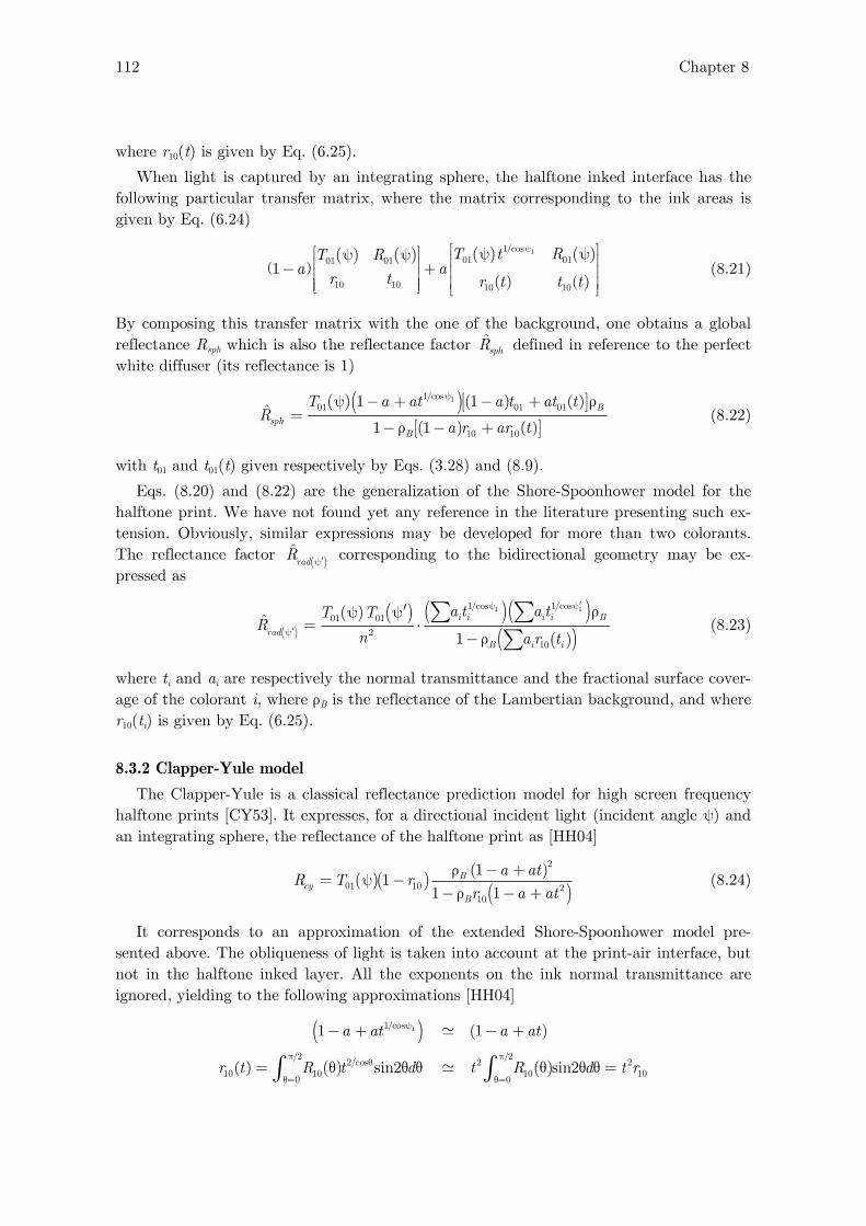
112 Chapter 8
where r10(t) is given by Eq. (6.25).
When light is captured by an integrating sphere, the halftone inked interface has the following particular transfer matrix, where the matrix corresponding to the ink areas is given by Eq. (6.24)
( )( ) ( ) ( ) ( )
( ) ( )
11/cos01 0101 01
10 10 10 10
1T t RT R
a ar t r t t t
ψ⎡ ⎤⎡ ⎤ ψ ψψ ψ ⎢ ⎥⎢ ⎥− + ⎢ ⎥⎢ ⎥ ⎢ ⎥⎢ ⎥⎣ ⎦ ⎣ ⎦ (8.21)
By composing this transfer matrix with the one of the background, one obtains a global reflectance Rsph which is also the reflectance factor sphR defined in reference to the perfect white diffuser (its reflectance is 1)
( )( )( ) ( )[ ]
( ) ( )[ ]
11/cos
01 01 01
10 10
1 1ˆ
1 1B
sphB
T a at a t at tR
a r ar t
ψψ − + − + ρ=
− ρ − + (8.22)
with t01 and t01(t) given respectively by Eqs. (3.28) and (8.9).
Eqs. (8.20) and (8.22) are the generalization of the Shore-Spoonhower model for the halftone print. We have not found yet any reference in the literature presenting such ex-tension. Obviously, similar expressions may be developed for more than two colorants. The reflectance factor ( )
ˆradR ′ψ corresponding to the bidirectional geometry may be ex-
pressed as
( )( ) ( ) ( )( )
( )( )
1 11/cos 1/cos01 01
210
ˆ1
i i i i B
radB i i
a t a tT TR
n a r t
′ψ ψ
′ψ
′ ρψ ψ= ⋅
− ρ∑ ∑
∑ (8.23)
where ti and ai are respectively the normal transmittance and the fractional surface cover-age of the colorant i, where ρB is the reflectance of the Lambertian background, and where r10(ti) is given by Eq. (6.25).
8.3.2 Clapper-Yule model
The Clapper-Yule is a classical reflectance prediction model for high screen frequency halftone prints [CY53]. It expresses, for a directional incident light (incident angle ψ) and an integrating sphere, the reflectance of the halftone print as [HH04]
( )( ) ( )
( )
2
01 10 210
11
1 1B
cyB
a atR T r
r a at
ρ − += ψ −
− ρ − + (8.24)
It corresponds to an approximation of the extended Shore-Spoonhower model pre-sented above. The obliqueness of light is taken into account at the print-air interface, but not in the halftone inked layer. All the exponents on the ink normal transmittance are ignored, yielding to the following approximations [HH04]
( ) ( )
( ) ( ) ( )
11/cos
/2 /22/cos 2 2
10 10 10 100 0
1 1
sin2 sin2
,
,
a at a at
r t R t d t R d t r
ψ
π πθ
θ= θ=
− + − +
= θ θ θ θ θ θ =∫ ∫

Compositional models for prints 113
( ) ( ) ( ) ( )
( ) ( ) ( )( ) ( ) ( )
/2 /21/cos
10 10 10 10 100 0
210 10 10
10 10 10
,
,
sin2 sin2
,
1
1
1
1 1
t t T t d t T d tt t r
a r ar t a at r
a t at t a at t
π πθ
θ= θ== θ θ θ θ θ θ = = −
− + − +
− + − +
∫ ∫
In their original paper, Clapper and Yule assume that these approximations have a very small effect on the accuracy of the reflectance predictions. This has been verified experimentally [HECC05]. The ink transmittance parameter, in the Clapper-Yule model, does not correspond precisely to a normal transmittance but rather to an average at-tenuation undergone by the diffuse light crossing the halftone ink layer.
8.3.3 Deducing dot surface coverages of paper from measurements
Once the intrinsic reflectance and transmittance of the printing support have been deduced from the reflectance and the transmittance of the unprinted printing support (see Sect. 7.1.4) and each colorant normal transmittance has been deduced from the reflec-tance and the transmittance of a print fully covered by the colorant, one can deduce the dot surface coverage from the measured reflectance and transmittance with single ink halftone patches.
For each ink, various patches are printed at different nominal coverages an. Their re-flectance spectrum is measured with a spectrophotometer using, for example, a bidirec-tional measuring geometry (incidence angle ψ and observation angle ψ′). The effective dot surface coverage a can be deduced from the global reflectance model, given by Eq. (8.20). Using a linear interpolation, one obtains an approximated correspondence between the nominal and the effective dot surface coverage (Fig. 8.3a).
0
1
1
0.25
0.25
0.5
0.5
Nominal surface coverage an
Effec
tive
surf
ace
cover
age
a
0.75
0.75 0 1
-0.1
0.25
0
0.5
Nominal surface coverage an
Dot
gai
n a−
an 0.1
0.75
(a) (b)
Fig. 8.3: (a) Nominal to effective dot surface coverage curve and (b) dot gain curve of cyan halftone patches printed at 180 lines per inch on white PVC sheets.
The dot gain, i.e. the difference na a− of nominal and effective coverages, is a function of the nominal coverage, generally different for each primary ink. In Fig 8.3b, we observe a

114 Chapter 8
negative dot gain, whereas dot gain is generally positive. Curves plotted in Fig. 8.3 have been obtained from patches printed with an offset press. The screen frequency, equal to 180 lines per inch, was higher than usual screen frequencies (150 lpi). Dot gain may have been overcompensated during the production of the offset films [Hir91], and the offset plate may have been overexposed during the insolation process, which is also calibrated for a frequency of 150 lpi.
8.3.4 Prediction of multi-ink halftone prints
When dot screens of various primary inks are superposed, the halftone inked layer comprises a certain number of colorants, having each one its normal transmittance ti and its dot surface coverage ai: no ink (also called “white” colorant), one primary ink (e.g. cyan, magenta, yellow), two superposed primary inks (e.g. red, green blue), three super-posed primary inks (e.g. polychromatic black).
Consider a halftone patch printed with nominal dot surface coverages C, M and Y. What is the reflectance spectrum that would be measured from such a patch? The predic-tion model relies on Eq. (8.20), expressing the reflectance factor ( )
ˆradR ′ψ of the print for a
bidirectional measuring geometry and a perfect white diffuser as reference. The following parameters should be determined:
− The spectral intrinsic reflectance ρB of the printing support, which is deduced from the measured reflectance of the unprinted printing support;
− The spectral normal transmittances ti of the different colorants, which are deduced from patches where each colorant is printed with a full surface coverage (see Sect. 8.1.2);
− The scalar (i.e. non-spectral) dot surface coverage ai of the colorants. Effective dot surface coverages of the colorants can be computed according to the method proposed by Hersch & al. [HER95] since the surface coverage of primary inks depends whether they are printed alone or superposed with other ink(s), due to the ink spreading phenomenon [EH02].
8.4 Reflectance and transmittance model for recto-verso halftone prints
Thanks to our general compositional model, one may easily develop a prediction model for transmittance of halftone prints, with a straightforward extension to recto-verso prints.
We consider here a symmetric printing support printed on both sides by two different halftones. The recto-verso print may be represented by a hexaface, whose external bifaces are the recto and the verso halftone inked interfaces, and whose central layer is the sub-strate layer of the printing support, assumed to be Lambertian. Considering the print as ideal (Sect. 8.2.1), the hexaface is regular since it does not contains any scattering biface (Sect. 5.2.1).
Since the recto and the verso have been printed during different offset print passes, respective ink thicknesses and surface coverages are slightly different between the recto and the verso. We therefore calibrate separately the recto and the verso inked layers. The parameters of the halftone inked layer (normal transmittance and effective surface cover-age of the colorants) are deduced from patches printed on the recto only (unprinted

Compositional models for prints 115
verso), and those of the verso inked layer are deduced from patches printed on the verso only (unprinted recto).
We consider the same measuring geometry as for the characterization of paper (Sect. 7.1) and ink (Sect. 8.1), i.e. a directional incident light (incidence angle ψ) and a radiance detector (observation angle ψ′) at the upper side, and a Lambertian illumination at the bottom side. This geometry enables measuring the upper reflectance Rrad(ψ′) and the lower transmittance Trad(ψ′) of the print.
8.4.1 Reflectance and transmittance model
The halftone inked interfaces are characterized by their fundamental transfer matrix, given by Eq. (8.15). Let us deduce their particular transfer matrix for the measuring ge-ometry specified above.
The upper halftone inked interface receives directional light on its upper face and Lambertian light on its lower face. Its upper face is also observed by the radiance detec-tor. According to formula (h) of Table 6.1, the transfer matrix of the upper inked inter-face is
( )
( )( ) ( )
( ) ( )
( )
( )( )
11
1 1 1
1/cos1/cos 01
01 01
2/cos 1/cos 1/cos01all 10 1 10 1 10 2
0diri i
i
ii i i i i i irad L
T a tT t Ra TR t T t a r t a t
n
ψψ →θ
θ θ ′ψ
′ψ ← ←
⎡ ⎤ψ⎧ ⎫⎡ ⎤⎪ ⎪θ θ ⎢ ⎥⎪ ⎪⎢ ⎥⎪ ⎪ ⎢ ⎥=⎨ ⎬⎢ ⎥ ′ ′⎢ ⎥ξ ψ⎪ ⎪⎢ ⎥θ θ⎪ ⎪ ⎢ ⎥⎣ ⎦⎪ ⎪⎩ ⎭ ⎢ ⎥π⎣ ⎦
∑∑
∑ ∑ (8.25)
where ti and ai are respectively the normal transmittance and the surface coverage of col-orants i printed on the recto.
The lower halftone inked interface is illuminated by Lambertian irradiances on its two sides. According to Eq. (6.2), it has the particular transfer matrix
( ) ( )
( ) ( )
( ) ( )( )
1 1
1
1/cos 2/cos10 10 1 10 10
1/cosall 01 01 1 01 01
L
i i i i i i
ii i i i
L
T t R t a t t a r ta
R T t r a t t
→ θ θ
θ
←
⎧ ⎫ ⎡ ⎤⎡ ⎤⎪ ⎪′ ′ ′ ′ ′ ′θ θ⎪ ⎪ ⎢ ⎥⎢ ⎥⎪ ⎪′ =⎨ ⎬ ⎢ ⎥⎢ ⎥⎪ ⎪′ ′ ′⎢ ⎥⎢ ⎥θ θ⎪ ⎪⎣ ⎦ ⎣ ⎦⎪ ⎪⎩ ⎭
∑ ∑∑
∑ (8.26)
where it ′ and ia ′ are respectively the normal transmittance and the surface coverage of the colorant printed on the verso, and where ( )10r t , ( )10t t and ( )01t t are given respectively by Eqs. (6.25), (6.32) and (8.9). By composing the upper inked interface, the symmetric paper layer and the verso inked interface,
( )
( )( )
( ) ( )( )
1
1
1/cos01
10 10
1/cos0101 0110 2
0
i i
i i i i
i ii i i i
T a t a t t a r t
T r a t ta r t a tn
ψ
′ψ
⎡ ⎤ψ ⎡ ⎤′ ′ ′ ′τ ρ⎢ ⎥ ⎡ ⎤ ⎢ ⎥⎢ ⎥ ⎢ ⎥ ⎢ ⎥′ ′⎢ ⎥ξ ψ ρ τ⎢ ⎥ ′ ′⎢ ⎥⎣ ⎦⎢ ⎥ ⎣ ⎦⎢ ⎥π⎣ ⎦
∑ ∑ ∑∑∑ ∑
(8.27)
and then by using the hexaface formula (5.27), we obtain the global reflectance of the recto-verso halftone print
( )
( ) ( ) ( ) ( )( ) ( ) ( ) ( )
1 11/cos 1/cos 2 201 01 10
2 210 10 10 101 1
i i i i i i
radi i i i i i i i
T T a t a t a r tR
n a r t a r t a r t a r t
′ψ ψ
′ψ
⎡ ⎤⎡ ⎤ ⎡ ⎤⎡ ⎤′ ′ ′ψ ψ ρ − ρ − τ′ ⎢ ⎥ ⎢ ⎥ξ ⎢ ⎥⎢ ⎥⎣ ⎦ ⎣ ⎦ ⎣ ⎦⎣ ⎦= ⋅⎡ ⎤ ⎡ ⎤⎡ ⎤ ⎡ ⎤′ ′ ′ ′π − ρ − ρ − τ⎢ ⎥ ⎢ ⎥⎢ ⎥ ⎢ ⎥⎣ ⎦ ⎣ ⎦⎣ ⎦ ⎣ ⎦
∑ ∑ ∑∑ ∑ ∑ ∑
(8.28)
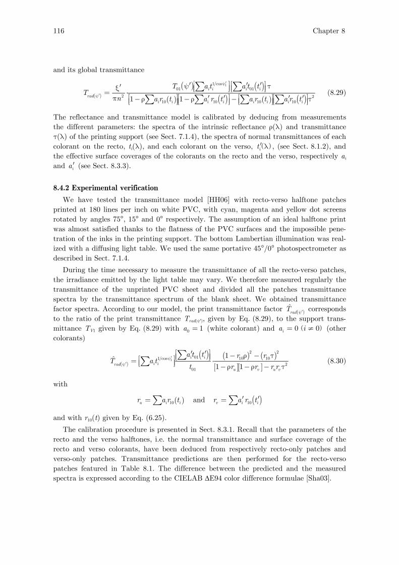
116 Chapter 8
and its global transmittance
( )
( ) ( )( ) ( ) ( ) ( )
11/cos01 01
2 210 10 10 101 1
i i i i
radi i i i i i i i
T a t a t tT
n a r t a r t a r t a r t
′ψ
′ψ
⎡ ⎤ ⎡ ⎤′ ′ ′ψ τ′ξ ⎢ ⎥ ⎢ ⎥⎣ ⎦ ⎣ ⎦= ⋅⎡ ⎤ ⎡ ⎤⎡ ⎤ ⎡ ⎤′ ′ ′ ′π − ρ − ρ − τ⎢ ⎥ ⎢ ⎥⎢ ⎥ ⎢ ⎥⎣ ⎦ ⎣ ⎦⎣ ⎦ ⎣ ⎦
∑ ∑∑ ∑ ∑ ∑
(8.29)
The reflectance and transmittance model is calibrated by deducing from measurements the different parameters: the spectra of the intrinsic reflectance ρ(λ) and transmittance τ(λ) of the printing support (see Sect. 7.1.4), the spectra of normal transmittances of each colorant on the recto, ti(λ), and each colorant on the verso, ( )
it ′ λ , (see Sect. 8.1.2), and the effective surface coverages of the colorants on the recto and the verso, respectively ai and ia ′ (see Sect. 8.3.3).
8.4.2 Experimental verification
We have tested the transmittance model [HH06] with recto-verso halftone patches printed at 180 lines per inch on white PVC, with cyan, magenta and yellow dot screens rotated by angles 75°, 15° and 0° respectively. The assumption of an ideal halftone print was almost satisfied thanks to the flatness of the PVC surfaces and the impossible pene-tration of the inks in the printing support. The bottom Lambertian illumination was real-ized with a diffusing light table. We used the same portative 45°/0° photospectrometer as described in Sect. 7.1.4.
During the time necessary to measure the transmittance of all the recto-verso patches, the irradiance emitted by the light table may vary. We therefore measured regularly the transmittance of the unprinted PVC sheet and divided all the patches transmittance spectra by the transmittance spectrum of the blank sheet. We obtained transmittance factor spectra. According to our model, the print transmittance factor ( )
ˆradT ′ψ corresponds
to the ratio of the print transmittance Trad(ψ′), given by Eq. (8.29), to the support trans-mittance TV1 given by Eq. (8.29) with 0 1a = (white colorant) and ( )0 0ia i= ≠ (other colorants)
( )
( ) ( ) ( )[ ][ ]
1
2 201 10 101/cos
201
1ˆ1 1
i i
i iradu v u v
a t t r rT a t
t r r r r′ψ
′ψ
⎡ ⎤′ ′ − ρ − τ⎢ ⎥⎣ ⎦⎡ ⎤= ⋅⎢ ⎥⎣ ⎦ − ρ − ρ − τ∑∑ (8.30)
with
( )10u i ir a r t= ∑ and ( ) 10v i ir a r t′ ′= ∑
and with r10(t) given by Eq. (6.25).
The calibration procedure is presented in Sect. 8.3.1. Recall that the parameters of the recto and the verso halftones, i.e. the normal transmittance and surface coverage of the recto and verso colorants, have been deduced from respectively recto-only patches and verso-only patches. Transmittance predictions are then performed for the recto-verso patches featured in Table 8.1. The difference between the predicted and the measured spectra is expressed according to the CIELAB ΔE94 color difference formulae [Sha03].

Compositional models for prints 117
Table 8.1: Difference (in CIELAB ΔE94) between predicted and measured transmittance spectra
for offset inks printed on white PVC.
Ink on the verso
C M Y R G B K C50 average
C 0.5 1.2 2.8 0.6 1.3 0.6 1.6 1.5 1.3
M 2.2 1.2 0.9 0.9 1.3 0.9 1.6 0.9 1.2
Y 1.0 0.7 0.5 0.8 0.9 0.3 1.6 1.3 0.9
R 2.3 0.8 0.4 0.7 1.5 1.1 1.4 0.4 1.1
G 0.5 0.5 2.6 0.7 0.8 0.4 3.3 2.3 1.4
B 2.1 1.0 0.2 1.8 1.6 1.2 1.1 1.4 1.3
K 2.0 1.6 0.4 1.5 0.7 1.5 1.4 1.7 1.4
C25 0.6 2.3 0.7 2.0 2.3 0.7 1.7 0.7 1.4
C50 0.5 2.0 1.6 1.9 2.0 1.1 2.5 0.8 1.6
Ink
on t
he r
ecto
C75 0.2 2.0 1.7 1.6 1.5 0.7 1.5 0.5 1.2
average 1.2 1.3 1.2 1.3 1.4 0.9 1.8 1.2 1.3
Legend: C stands for cyan solid inked layer, M for solid magenta, Y for solid yellow, R for super-posed magenta and yellow solid inks yielding the red colorant, G for solid yellow and cyan (greencolorant), B for solid cyan and magenta (blue colorant), K for the superposed cyan, magenta andyellow solid inks (black colorant); C25, C50 and C75 stand for cyan halftones of respective nominalsurface coverages 0.25, 0.5 and 0.75.
The mean difference between the measured transmission spectra and the transmission spectra predicted according to the recto-verso model is ΔE94 = 1.3. Almost 90% of the predicted transmittance spectra have a ΔE94 prediction error of less than 2, which corre-sponds to the normal offset printing accuracy. This experiment shows that the prediction accuracy that is achieved by the proposed model for transmittance spectra is excellent. It is similar to the prediction accuracy of reflection spectra that is achieved for recto only offset prints by the classical Clapper-Yule model [HECC05].
Summary
We have applied the compositional model to the characterization of prints. The ink transmittance can be deduced for each wavelength from the measurement of the global reflectance spectrum or the global transmittance spectrum of a patch printed with a solid ink layer. Both possibilities yields the same transmittance spectrum. The notion of biface and the Shore-Spoohower model have been extended to halftone inked layers with high screen frequency. We have shown that the classical Clapper-Yule model is an approxima-tion of this model.
We have also developed a model for recto-verso multi-ink halftone print, experimen-tally validated with solid colorant patches and cyan halftones. The difference between measured and predicted spectra, expressed in CIELAB ΔE94, is 1.3, which is less than the threshold of the human eye perception. In the future, in order to predict accurately

118 Chapter 8
the reflectance and the transmittance multi-ink recto-verso halftone patches, the ink spreading phenomenon shall be taken into account according to the model proposed by Hersch & al. [HECC05].

119
Conclusion
We presented a general model of multilayer reflectance and transmittance relying on geometrical optics and using a hierarchical description of the interaction of light with the different layers and interfaces forming the multilayer specimens. In the most general case, a step by step description of the multiple reflection-transmission of light in the multilayer yields a reflectance and a transmittance expressed as infinite sums. However, when the multilayer does not contain any rough interface or any weakly scattering layer (i.e. no scattering biface), or when each of these interfaces or layers is directly bordered by a strongly scattering layer, the step-by-step description can be avoided. Instead, we have advocated the use of closed-form formulae, called “compositional formulae”, including the full multiple reflection-transmission process. We have introduced a special formalism al-lowing to derive in a straightforward manner the particular reflectance and transmittance that should be associated with each face. The geometries of the light sources and the cap-turing devices are included in this special formalism. Thanks to the notion of composition and the composition formulae, the establishment of multilayer reflectances and transmit-tances of multilayer specimens is considerably simplified.
The soundness of our approach has been proven by its ability to retrieve Kubelka’s model, the Williams-Clapper model, the Saunderson correction, and the Clapper-Yule model. New models have also been developed that would have been very difficult to con-ceive without our compositional formalism. The new noncontact double sheet model per-mits to exclude the influence of the measuring geometry on the deduction of the paper intrinsic parameters. The prediction model for high screen frequency recto-verso halftone prints, verified experimentally, has an excellent accuracy.
In the future, we intent to check the relevance of the parameters deduced using the Clapper-Yule model, which is based on approximated equations (see Sect. 8.3.2). We also intent to verify to which extent, in low quality prints, interfaces can be considered as flat and inks can be considered as transparent without loss of the prediction accuracy. Thanks to the transmittance model, we now have enough equations for ascertaining parameters and exploring phenomena such as the light scattering inside the inks. In a further step, we may increase the number of measurement configurations, both in reflectance and transmittance mode, thanks to known filters. By composing the bifaces of the filters with the bifaces of the specimen, it will be possible to obtain new equations for parameter fit-tings without having to introduce additional unknown parameters.


121
Appendix A.
Complements of radiometry
A.1 Relationship between reflectance and BRDF
The reflectance of a material is defined for an incident flux angularly distributed ac-cording to a radiance function Li, for a given solid angle of incidence Γi, and for a given solid angle of observation Γr (see Sect. 1.2.2). The following detailed calculation estab-lishes the relationship between reflectance and BRDF.
Let us first take one direction within the incidence solid angle Γi, denoted by the dif-ferential solid angle sini i i id d dω = θ θ φ . We consider a radiance ( )i iL dω at the selected di-rection idω . The incident element of irradiance ( )i idE dω , given by Eq. (1.7), is
( ) ( ) cosi i i i i idE d L d dω = ω θ ω (A.1)
Let us also consider one direction within the observation solid angle Γr, denoted by the differential solid angle sinr r r rd d dω = θ θ φ . The radiance reflected in this direction is the product of the incident element of irradiance dEi by the bidirectional reflectance distribu-tion function fR [Eq. (1.14)]
( ) ( ) ( ) ,r r R i r i iL d f d d dE dω = ω ω ω (A.2)
In order to obtain the reflectance i r
RΓ →Γ , we must take into account all the directions of incidence within Γi and all the directions of observation within Γr. On the one hand, the reflected radiance ( )r rL dω corresponds to the reflected element of flux ( )2 ,r i rd d dΦ ω ω con-sidered with respect to the surface element ds and the infinitesimal solid angle rdω
( )( )
2 ,
cosr i r
r rr r
d d dL d
ds d
Φ ω ωω =
θ ω (A.3)
The combination of Eqs. (A.1), (A.2) and (A.3) yields
( ) ( ) ( )
2 , , cos cosr i r R i r i i i i r rd d d dsf d d L d d dΦ ω ω = ω ω ω θ ω θ ω (A.4)
The double sum of the reflected elements of flux ( )2 ,r i rd d dΦ ω ω over the incidence solid angle Γi and over the observation solid angle Γi yields the total flux rdΦ reflected within the cone Γr
( ) ( ) , cos cosi i
r r
dr R i r i i i i r rd
d ds f d d L d d dω ∈Γω ∈Γ
Φ = ω ω ω θ ω θ ω∫∫ (A.5)
On the other hand, the total incident flux idΦ is the sum over Γi of the directional ele-ments of flux ( ) ( )2
i i i id d dE d dsΦ ω = ω

122 Appendix A
( ) cosi i
i i i i id
d ds L d dω ∈Γ
Φ = ω θ ω∫ (A.6)
The ratio /r id dΦ Φ , issued from Eqs. (A.6) and (A.5), corresponds to reflectance i r
RΓ →Γ
( ) ( )
( )
, cos cos
cosi i r r
i r
i i
R i r i i i i r rd d
i i i id
f d d L d d dR
L d d
ω ∈Γ ω ∈ΓΓ →Γ
ω ∈Γ
ω ω ω θ ω θ ω=
ω θ ω
∫ ∫∫
(A.7)
A.2 Reflectance and transmittance measured with a radiance detector
A radiance detector receives an element of flux d2Φd perpendicularly incident on its surface dsd through its solid angle dΩd, assumed to be small. In spectral prediction models, it is generally, convenient to consider the measured radiance Ld instead of the measured flux. The ratio of the measured radiance to the incident irradiance defines a pseudo-reflectance or a pseudo-transmittance. We propose here to establish the relationship exist-ing between these quantities and the exact reflectance and transmittance, defined as ratio of fluxes.
The measured radiance is
2
dd
d d
dL
ds dΦ
=Ω
(A.8)
According to the radiance invariance principle (see Sect. 1.1.3), radiance Ld is equal to the radiance L emitted by the specimen in the direction of the detector. This radiance is de-fined by the solid angle 2/dd ds xω = subtended by the detector’s surface, where x is the distance between the detector and the specimen, and by the specimen’s element of area
2/cosdds d x= Ω θ , where θ is the angle formed by radiance L with the specimen’s normal (Fig. A.1)
dω
dΩd
N
dsd
ds
Radiance detector
x
θ
Fig. A.1: Radiance invariance between the radiance detector and an elemental area on the specimen.

Appendix A 123
According to the transfer volume conservation principle (see Sect. 1.1.3), one has
cosd dds d dsdΩ = ω θ (A.9)
Elemental area ds receives an incident element of flux d2Φi. The incident irradiance is
2 /i iE d ds= Φ (A.10)
The relationship between the ratio Ld/Ei and the ratio d2Φd/d2Φi may be deduced from
Eqs. (A.8), (A.9) and (A.10)
2
2 2
cos cosd d d d d d d
i i i i
d L ds d L dsd ds Ld E ds E ds x E
Φ Ω ω θ θ= = = ⋅
Φ (A.11)
Eq. (A.11) indicates that, for a fixed orientation θ of the detector, the ratio Ld/Ei is pro-portional to the ratio d2Φd/d
2Φi, i.e. it is proportional to a reflectance, called Rrad. The coefficient of proportionality
2cos /dds xξ = θ (A.12)
is called the “apparatus constant” of the detector. It is a function of the angle of observa-tion θ, the detector’s area dsd and the distance x between the detector and the specimen. The relationship between Rrad and the ratio Ld/Ei is therefore
drad
i
LR
E= ξ ⋅ (A.13)
Let us now consider a perfect white diffuser. It is a Lambertian reflector of reflectance equal to 1. The ratio (Ld/Ei)ref is equal to 1/π, and the reflectance of this reference reflec-tor is
/refR = ξ π (A.14)
By dividing the specimen’s reflectance by the reference reflectance, coefficient ξ cancels. The ratio /rad refR R defines the reflectance factor radR of the specimen in reference to the perfect white diffuser
ˆ rad drad
ref i
R LR
R Eπ
= = (A.15)
A.3 Cosine correction in measures of BRDFs
A goniophotometer is composed of a directional light source and a radiance detector allowing measuring bidirectional reflectances for any direction of incidence and any direc-tion of observation. We assume that the detector belongs to the incidence plane.
The directional light source emits a radiance Li in the direction perpendicular to its surface dss, within a solid angle dΩs (Fig. A.2). Radiance Li intercepts an area dAs on the specimen. Elemental areas dss and dAs are distant by a length x (length of the rotating arm of the goniophotometer). According to the radiance invariance principle, the radiance

124 Appendix A
received by dAs, through the solid angle dωi subtended by dss, is equal to Li
2 2
cosi i
is s s i i
d dL
ds d dA dΦ Φ
= =Ω θ ω
(A.16)
with 2s
i
dsd
xω = and
2
coss
si
d xdA
Ω=
θ (A.17)
The element of irradiance dEi(θi) illuminating dAs is
( ) 2cos cos si i i i i i i
dsdE L d L
xθ = θ ω = θ (A.18)
dωr
dΩd
dωi
dΩs
θi
N
dsd
dss
dAddAs
Radiance detector
Light source
x
x θr
Fig. A.2: The radiance emitted by the light source through its solid angle dΩs il-luminates a portion dAs of the specimen. A portion dAd < dAs is observed by the detector through its solid angle dΩd.
The radiance detector receives the reflected flux ( )2d rd Φ θ through its solid angle dΩd per-
pendicularly to its surface dsd. It measures the radiance Ld expressed by Eq. (A.8). The solid angle dΩd of the detector intercepts an area dAd on the specimen. The illuminated area dAs and the observed area dAd are different.
Let us first consider, as in Fig. C.1, that dAs > dAd. Since the incident light is direc-tional, dAs and dAd both receive the same radiance Li and thereby the same element of irradiance dEi(θi), given by Eq. (A.18). According to the radiance invariance principle, the radiance Ld captured by the detector at angle θr is equal to the radiance ( )r rL θ reflected by dAd towards the detector
( )( ) ( )
2 2
cosd r
d r d rr r
d r r d d
L L
d dL
dA d ds d
Φ θ Φ θθ = =
θ ω Ω (A.19)
Hence, the BRDF fR, defined as the ratio of the reflected radiance to the incident element

Appendix A 125
of irradiance ( )i idE θ is
( )( )( )
( )
2
2
,cos
r r d rR i r
si id d i i
L df dsdE ds d L
x
θ Φ θθ θ = =
θ Ω θ (A.20)
Considering a fixed angle of incidence θi, the denominator
2cos /d d i i sds d L ds xΩ θ is a con-stant. The BRDF is proportional to the flux captured by the radiance detector
( ) ( )
2,R i r d rf kdθ θ = Φ θ (A.21)
Eq. (A.21) relies on the assumption that the observed area dAd is completely illumi-nated, i.e. dAs > dAd. Let us now assume that, at a certain angle of observation, dAd be-comes larger than dAs (Fig. A.3).
dΩddΩs
Ndsd
dss
dω
dAddAs
Radiancedetector
Light source
θrθi
Fig. A.3: The area dAd observed by the detector is larger than the area dAi illu-minated by the light source. The solid angle dω through which the detector re-ceives light is lower than its own solid angle dΩd.
The solid angle dω through which the detector receives light from the illuminated area on the specimen, i.e. from dAs given by Eq. (A.17), is
2
cos coscos
s r rs
i
dAd d
xθ θ
ω = = Ωθ
(A.22)
The radiance Ld captured by the detector thus becomes
( ) ( )
2 2 cos
cosd r d r i
dd d s r
d dL
ds d ds d
Φ θ Φ θ θ= =
ω Ω θ (A.23)
Ld is equal to the reflected radiance ( )r rL θ according to the radiance invariance principle. The specimen’s BRDF is therefore

126 Appendix A
( )( )( )
( )( )
2
2,
cos /r r d r
R i ri i d s r i s
L df
dE ds d L ds x
θ Φ θθ θ = =
θ Ω θ (A.24)
Like previously, the term 2/d s i sds d Lds xΩ is a constant. However, there remains a term cosθr. The flux captured by the detector is proportional to the BRDF multiplied by the cosine of the observation angle
( ) ( ) ′Φ θ = θ θ θ2 , cosd r R i r rd k f (A.25)
In practice, the light source is positioned at a fixed angle θi and the detector rotates around the specimen from observation angles 0 to π/2. As the observation angle θr in-creases, the observed area also increases. If at θr = 0 the observation area is fully illumi-nated by the incident light beam, there exists an angle θlim at which the illuminated and observed areas will be equal. At angles below θlim, the BRDF is given by Eq. (A.21), and at angles higher than θlim, the BRDF is given by Eq. (A.25). We may therefore introduce a correction function C permitting to convert the measured flux into the BRDF
( ) ( ) ( )
2, ,R i r i r d rf C dθ θ = θ θ Φ θ (A.26)
with
( )
lim
lim lim
1 0for,
forcos /cos /2
r
i rr r
C⎧ ≤ θ ≤ θ⎪⎪⎪θ θ = ⎨⎪ θ θ θ ≤ θ ≤ π⎪⎪⎩
(A.27)
Angle θlim can be determined experimentally. A Lambertian reflector, whose BRDF is con-stant, is selected. The arm of the goniophotometer carrying the directional light source is placed at a selected angle. The other arm, carrying the radiance detector, moves in the incidence plane from the normal of the specimen (0 degree) to the horizontal direction (90 degrees). The curve of the flux captured by the detector, expected to be a constant func-tion, should rather have the shape featured in Fig. A.4. Angle θlim is the abscissa from which the curve decreases according to a cosine curve.
ΦL(θ)
0° 90° θθlim
Fig. A.4: Curve of the flux ( )Φ θd measured by the gonio-photometer from a Lambertian reflector.
Remark: the minimal observed area, obtained for the observation θr = 0, may yet be lar-ger than the illuminated area. In this case, one has θlim = 0. The curve of the flux meas-ured from a Lambertian reflector will have a perfect cosine shape.
Φd(θ)

127
Appendix B.
Markov chains
Multiple reflection-transmission of light occurring in a regular multiface may be repre-sented by Markov chains. We propose to recall here basic elements of the general theory of Markov chains, mainly borrowed from [Ste94] and [MT73] (Sect. B.1, B.2 and B.3). We then focus on absorbing Markov chains on which relies the compositional model (Sect. B.4).
B.1 Definition of a Markov chain
A Markov chain is a convenient representation of the behavior of a physical system which describes the different states that the system may occupy and indicates how the system moves from one state to another in time [Ste94].
Consider a system that may occupy a finite number of states. Random variables Y0, Y1, Y2,…, Yn give the respective state y0, y1, y2,…,yn in which the system is at discrete “times” 0, 1, 2,…, n. A sequence y0, y1, y2,…,yn of states corresponds to a certain realiza-tion of a random walk. The probability m that this realization occurs is the conditional probability that the irradiance is observed in state yn at time n, given that it was previ-ously observed in states y0, y1 … yn–1 respectively at times 0, 1,…,n–1
0 0 1 1Prob ,...,n n n nm Y y Y y Y y− −= = = = (B.1)
This conditional probability m can also be interpreted as the probability of transition from state yn–1 to state yn, given that it has previously moved from state y0 to state y1, from state y1 to state y2, etc. When the transition probability 1n ny y− → is independent of the previous transitions 0 1y y→ , 1 2y y→ , … 2 1n ny y− −→ , the stochastic process is said to be memoryless. This may be written as
0 0 1 1 1 1Prob ,..., Probn n n n n n n nY y Y y Y y Y y Y y− − − −= = = = = = (B.2)
Equality (B.2) is the defining equation of a discrete-time Markov chain. When, further-more, the transition probabilities 1n ny y− → are independent of the time parameter n, the Markov chain is said to be a homogenous discrete-time Markov chain (HDMC). Hence, if the system is in a given state i, it evolves towards a given state j with a same probability whatever the time and whatever the previous states in which the system has been through.
B.2 Probability transition matrices
Let us consider a homogenous discrete-time Markov chain and two of its states i and j. The probability of transition from state i to state j is a constant (independent of the time

128 Appendix B
parameter n), called single-step transition probability and noted mij
1Probij n nm Y jY i−= = = (B.3)
Matrix ijm=M is called the single-step transition probability matrix associated with the chain. M is a square matrix whose size corresponds to the number of states in the chain. Since elements mij are probabilities, they satisfy the inequality
0 1ijm (B.4)
The single-step transition probability matrix, which satisfies (B.4), is said to be a non-negative matrix. Furthermore, the sum of its row elements is less than 1, i.e. for all i,
1ijj
m∑ (B.5)
We may generalize a single-step transition probability matrix to a k-step transition prob-ability matrix M(k) whose elements ( )k
ijm are probabilities for transitions from a state i to a state j in k steps
( ) Probkij n k nm X j X i+= = = (B.6)
These elements may be obtained from the single-step transition probabilities. It may be first seen that ( )1
ij ijm m= . The Markov property, expressed by Eq. (B.2), gives the follow-ing recursive formula for the ( )k
ijm
( ) ( ) ( )
all
, for 0 .k ppkij iq qj
q
m m m l n−= < <∑ (B.7)
Relation (B.7) is called the Chapman-Kolmogorov equation for the Markov chain. In ma-trix notation, the Chapman-Kolmogorov equations are written as
( ) ( ) ( )k ppk −=M M M
Note in particular that
( ) ( ) ( )1 1k kk − −= =M M M MM (B.8)
Hence, the matrix on k-step transition probabilities is obtained by multiplying (k−1) times the single-step transition probability matrix by itself, i.e.
( )k k=M M (B.9)
An “infinite-step” transition probability matrix M∞ can be as well defined by
lim k
k∞ →∞
=M M (B.10)
Like the single-step, k-step and infinite-step transition probability matrices are nonnega-tive matrices and are independent of the time parameter n.

Appendix B 129
B.3 Properties of nonnegative, stochastic and substochastic matrices
Transition probability matrices are basically square matrices, which may be character-ized by their spectral radius, i.e. their largest eigenvalue modulus. Given a square matrix A having a spectrum composed of the eigenvalues ( )jλ A , its spectral radius ( )R A is de-fined as
( ) ( )max j jR = λA A (B.11)
It can be shown that for any natural matrix norm ⋅
( )R A A (B.12)
It is true in particular for the matrix infinity-norm, defined as the maximum absolute row sum
( )
all
max iji
j
a∞ = ∑A (B.13)
In the case of transition probability matrices, it follows property (B.5) that
( ) 1R ∞A A (B.14)
Thus, all eigenvalues of a transition probability matrix have their modulus at most 1. This will be stated in the following paragraphs.
B.3.1 Non-Negative matrices
Nonnegative matrices are matrices whose elements are also positive or zero. Transition probability matrices are therefore nonnegative [Eq. (B.4)].
A nonnegative matrix A is said to be decomposable if it can be brought by a symmet-ric permutation of its rows and its columns to a triangular block matrix, i.e. if a permuta-tion matrix P exists such that
T⎛ ⎞⎟⎜ ⎟⎜ ⎟⋅ ⋅ = ⎜ ⎟⎜ ⎟⎜ ⎟⎝ ⎠
U WP A P
0 V (B.15)
where U and V are square nonzero matrices and W is, in general, rectangular.
B.3.2 Stochastic and substochastic matrices
A nonnegative matrix A is said to be a stochastic matrix if it satisfies the following two conditions
1. all
1ijja =∑ for all i.
2. At least one element in each column differs from zero.
Condition (1) implies that a transition is guaranteed to occur from state i to at least one state in the next time (that may be state i again). Condition (2) specifies that since each column has at least one nonzero element, there are no ephemeral states, i.e., states that

130 Appendix B
could not possibly exist after the first time transition. This second condition is generally omitted, being considered as trivial.
Nonnegative matrix A is substochastic if, instead of satisfying condition (1) above, it satisfies
1ijj
a∑ (B.16)
Remark: In the context of multiple reflection-transmission processes, the physical inter-pretation of a stochastic process is the fact that each face redistributes completely the light it receives by reflection and transmission, without absorption. If light is absorbed by a certain face, one obtains
1ijj
a <∑ (B.17)
for the row i corresponding to that face, responsible of the substochasticity of A.
Property B.1: The spectral radius of stochastic matrices is one.
Proof: Let A be a nondecomposable stochastic matrix. Its spectral radius is
( ) ( )
all
max iji
j
R a∞ = ∑A A (B.18)
Owing to the defining condition (1) of stochastic matrices, one has 1∞ =A and there-fore ( ) 1R A . Since the sum of the elements of each of its rows is equal to 1, one has
=Ae e (B.19)
with ( )1,1,...,1 T=e . It immediately follows that 1 is an eigenvalue of A and that ( ) 1R =A . á
Property B.2: The spectral radius of substochastic matrices is strictly less than one.
Proof: Let ija=A be a nondecomposable substochastic matrix. Following the same reasoning line than for stochastic matrices, one may show that ( ) 1R A . Let us now show that 1 cannot be an eigenvalue of A. A being substochastic, at least one of its rows has a sum strictly less than 1, i.e. a number i0 exists such that
0
1i jj
a <∑ (B.20)
Should 1 be an eigenvalue of A, then a vector [ ]1 2, ,..., nx x x=X would exist such that
=X XA (B.21)
i.e., for all j
j ij ii
x a x= ∑ (B.22)

Appendix B 131
Let us perform the sum of the xj
( ) ( )
0 0
0
j ij i ij i i j ij j i i i j j
x a x a x a x≠
= = +∑ ∑∑ ∑ ∑ ∑ (B.23)
From inequality (B.20), one would obtain the following contradiction
j ij i
x x<∑ ∑ á (B.24)
Lemma B.1: Let A be a substochastic matrix. It satisfies
lim k
k→∞=A 0 (B.25)
and
( ) 1
0
k
k
∞−
=
= −∑A I A (B.26)
where 0 and I are respectively the zero matrix and the identity matrix having the same size as A. Eq. (B.25) generalizes the well-known scalar geometric series formulate
0
11
k
k
xx
∞
=
=−∑ (B.27)
In order to give a precise meaning to (B.26), one must first make sure that the series k∑A has a thorough meaning.
Let 1 21 ... n> λ λ λ be the eigenvalues of A. If A is diagonalizable, there exists an invertible matrix Q such that
( )
1
1 11,..., n
n
diag− −
⎛ ⎞λ ⎟⎜ ⎟⎜ ⎟⎜ ⎟⎜ ⎟= ⋅ ⋅ = ⋅ λ λ ⋅⎜ ⎟⎜ ⎟⎟⎜ ⎟⎜ ⎟λ⎜ ⎟⎝ ⎠
A Q Q Q Q (B.28)
Therefore,
( ) 11 ,...,
k k kndiag −= ⋅ λ λ ⋅A Q Q (B.29)
Since every |λi| is strictly less than 1, entries kiλ of the diagonal matrix in Eq. (B.29) de-
creases towards zero as the exponent k increases, which gives Eq. (B.25). Furthermore, for all i, one can sum up
0
11
ki
k i
∞
=
λ =− λ∑ (B.30)
From Eqs. (B.29) and (B.30), one has
( ) ( ) ( )
( )
2 2 1
0
1 1 11
... ...
,...,
Nk N
k
N Nndiag
+
=
+ + −
− = + + + − ⋅ + + + = −
= − ⋅ λ λ ⋅
∑I A A I A A A I A A I A
I Q Q

132 Appendix B
Since all the eigenvalues of A are strictly less than 1, one has
( )1 11lim ,...,N N
nN
diag + +
→∞λ λ = 0
and therefore
( )0
limN
k
Nk
→∞=
− =∑I A A I (B.31)
which finally yields Eq. (B.26). We conclude that the radius of convergence of matrix series is given by ( ) 1R <A , where ( )R A is the matrix spectral radius.
B.4 Absorbing Markov chains
The ith state of a Markov chain is said to be absorbing if 1iim = . It follows immedi-ately relation (B.5) that ( )0, ijm j i= ≠ . The set of conditions 1iim = and 0,ijm = ( )j i≠ is the mathematical statement expressing that once the system has reached state i, it never leaves anymore that state. A Markov chain is said to be absorbing if
1. There is at least one absorbing state,
2. There exists a transition (possibly in several steps but with a nonzero probability) from each nonabsorbing states to some absorbing state.
In studying absorbing chains, it is convenient to adopt certain conventions regarding the labeling of the states. Let us agree that the states are numbered in such a way that ab-sorbing states are placed at the last positions. Then, if the chain contains N absorbing states, the single-step transition probability matrix M has the form [Mey00, p. 700]
N
⎛ ⎞⎟⎜ ⎟⎜= ⎟⎜ ⎟⎜ ⎟⎜⎝ ⎠
A BM
0 I (B.32)
where A is a square matrix whose elements are the probabilities of transition from a non-absorbing state to a nonabsorbing state, B is a rectangular matrix having N columns whose elements are probabilities of transition from a nonabsorbing state to an absorbing state, 0 is a rectangular block of zeros having N rows, and IN is the N×N identity matrix. Note that, according to the defining property 2 of absorbing chains, B is a nonzero matrix and A is consequently a substochastic matrix.
According to Eq. (B.9) and the block decomposition (B.32), one may write the 2-step transition probability matrix as
2
2
N N N
⎛ ⎞⎛ ⎞ ⎛ ⎞ + ⎟⎟ ⎟ ⎜⎜ ⎜ ⎟⎟ ⎟ ⎜⎜ ⎜ ⎟⎟ ⎟= ⋅ = ⎜⎜ ⎜ ⎟⎟ ⎟ ⎜⎜ ⎜ ⎟⎟ ⎟ ⎜⎜ ⎜ ⎟⎟ ⎟ ⎟⎜⎝ ⎠ ⎝ ⎠ ⎝ ⎠
A B A B A AB BM
0 I 0 I 0 I (B.33)
The 3-step transition probability matrix may be written as
2 3 2
3
NN N
⎛ ⎞ ⎛ ⎞⎛ ⎞+ + +⎟ ⎟⎟⎜ ⎜⎜⎟ ⎟⎟⎜ ⎜⎜⎟ ⎟⎟= ⋅ =⎜ ⎜⎜⎟ ⎟⎟⎜ ⎜⎜⎟ ⎟⎟⎜ ⎜⎜⎟ ⎟⎟⎟ ⎟⎜ ⎜⎝ ⎠⎝ ⎠ ⎝ ⎠
A BA AB B A A B AB BM
0 I0 I 0 I (B.34)

Appendix B 133
Pursuing iteratively the products of Mk by M, one would obtain the following k-step tran-sition probability matrix
1
0
kk j
k j
N
−
=
⎛ ⎞⎟⎜ ⎟⎜ ⎟⎜ ⎟⎜= ⎟⎜ ⎟⎜ ⎟⎟⎜ ⎟⎜ ⎟⎜⎝ ⎠
∑A A BM
0 I
(B.35)
and thereby, according to its defining equation (B.10), the following infinite-step transi-tion probability matrix
0
lim k j
kj
N
∞
→∞=
∞
⎛ ⎞⎟⎜ ⎟⎜ ⎟⎜ ⎟⎜= ⎟⎜ ⎟⎜ ⎟⎟⎜ ⎟⎜⎝ ⎠
∑A A BM
0 I (B.36)
A being a substochastic matrix, it satisfies Eqs. (B.25) and (B.26). Thus, Eq. (B.36) be-comes [Mey00, p. 701]
( ) 1
N
−
∞
⎛ ⎞− ⎟⎜ ⎟⎜ ⎟= ⎜ ⎟⎜ ⎟⎜ ⎟⎟⎜⎝ ⎠
0 I A BM
0 I (B.37)
where I is the identity matrix having the size of A.


135
Appendix C.
Compositional formulae
In Chapter 5, we stated that the global transfer matrix of a regular multiface is the upper-right block of the infinite transfer matrix M∞ associated to the Markov chain repre-senting the multiface (see Eq. (5.22)). Since the Markov chain is absorbing (the states associated to the detectors are absorbing states, as seen in Sect. 5.2.3), we can directly use Eq. (B.37). Let us compute the transfer matrices of the quadriface and the hexaface presented in Sect. 5.3.1 and Sect. 5.3.2, yielding the quadriface and the hexaface formulae.
C.1 Quadriface formula
In Sect. 5.3.1, we presented a quadriface whose global transfer matrix G is defined by the composition equation
U U u u v v
u u v vV V
T R p s x r
r x s pR T
⎡ ⎤ ⎡ ⎤ ⎡ ⎤⎢ ⎥ ⎢ ⎥ ⎢ ⎥= =⎢ ⎥ ⎢ ⎥ ⎢ ⎥⎣ ⎦ ⎣ ⎦⎢ ⎥⎣ ⎦G (C.1)
The corresponding Markov chain, represented in Fig. 5.6, has the single-step transition probability matrix [see Eq. (5.17)]
=M
0 0 0 00 0 0 00 0 0 00 0 0 00 0 0 0 1 00 0 0 0 0 1
u u
v v
v v
u u
p sp sr x
r x
⎛ ⎞⎟⎜ ⎟⎜ ⎟⎜ ⎟⎜ ⎟⎜ ⎟⎜ ⎟⎟⎜ ⎟⎜ ⎟⎜ ⎟⎜ ⎟⎜ ⎟⎜ ⎟⎜ ⎟⎟⎜ ⎟⎜ ⎟⎜ ⎟⎟⎜⎝ ⎠
(C.2)
Let us decompose M like in Eq. (B.32). Matrices A and B are subsequently decomposed into 2×2 blocks
M =
0
0
0
0
0
0
up⎛ ⎞⎟⎜ ⎟⎜ ⎟⎜ ⎟⎜ ⎟⎜ ⎟⎜ ⎟⎟⎜ ⎟⎜ ⎟⎜ ⎟⎜ ⎟⎜ ⎟⎜ ⎟⎜ ⎟⎜ ⎟⎟⎜ ⎟⎜ ⎟⎜ ⎟⎜ ⎟⎜ ⎟⎟⎜⎝ ⎠
=
0
0
0
0
0
0
up⎛ ⎞⎟⎜ ⎟⎜ ⎟⎜ ⎟⎜ ⎟⎜ ⎟⎜ ⎟⎟⎜ ⎟⎜ ⎟⎜ ⎟⎜ ⎟⎜ ⎟⎜ ⎟⎜ ⎟⎜ ⎟⎟⎜ ⎟⎜ ⎟⎜ ⎟⎜ ⎟⎜ ⎟⎟⎜⎝ ⎠
=
0 0 0 0
0 0 0 0
0 0 0 0
0 0 0 0
0 0 0 0 1 0
0 0 0 0 0 1
u u
v v
v v
u u
p s
p s
r x
r x
⎛ ⎞⎟⎜ ⎟⎜ ⎟⎜ ⎟⎜ ⎟⎜ ⎟⎜ ⎟⎟⎜ ⎟⎜ ⎟⎜ ⎟⎜ ⎟⎜ ⎟⎜ ⎟⎜ ⎟⎜ ⎟⎟⎜ ⎟⎜ ⎟⎜ ⎟⎜ ⎟⎜ ⎟⎟⎜⎝ ⎠
(C.3)
with the following meaning for the different blocks: P contains the penetration transmit-tances of the upper and the lower bifaces, S their external reflectances, R their internal reflectances and X their exit transmittances. Let us note that either ru or rv is strictly less than 1. Otherwise, would ru = rv = 1, one would have xu = xv = 0 due to (B.16), which would mean that light cannot exit the multiface. Hence, block A is a substochastic matrix
B A
024 I
0
0
0 0 I
X R
P S

136 Appendix C
(see Sect. B.3).
The global transfer matrix G is the upper-right 2×2 block of M∞. According to Eq. (B.37), G is the upper 2×2 block of (I4 –A)–1B
( ) 14
−⎛ ⎞⎟⎜ ⎟ = −⎜ ⎟⎜ ⋅ ⎟⎟⎜⎝ ⎠
GI A B (C.4)
where the point represents an unspecified 2×2 block. One can write, using (C.3),
( )4
⎛ ⎞− ⎟⎜ ⎟⎜− = ⎟⎜ ⎟⎜ ⎟⎜⎝ ⎠−
I PI A
0 I R (C.5)
and, using a straightforward block computation,
( )
1
1
( )−
−
⎛ ⎞⎛ ⎞ ⎛ ⎞− − ⎟⎜⎟ ⎟⎜ ⎜⎟⎟ ⎟⎜⎜ ⎜⎟⎟ ⎟⋅ =⎜⎜ ⎜⎟⎟ ⎟⎜⎜ ⎜⎟⎟ ⎟⎜− ⎟⎜ ⎜⎟ ⎟− ⎟⎜⎝ ⎠ ⎝ ⎠⎝ ⎠
I P I 0I P I R
0 I R 0 I0 I R (C.6)
Therefore,
( )( )
( )
1
14 1
−
−
−
⎛ ⎞− ⎟⎜ ⎟⎜ ⎟− = ⎜ ⎟⎜ ⎟⎜ ⎟− ⎟⎜⎝ ⎠
I P I RI A
0 I R (C.7)
Then, using the decomposition of B as a function of blocks S and X, one has
( )( )
( )
( )
( )
1 1
14 1 1
− −
−
− −
⎛ ⎞ ⎛ ⎞⎛ ⎞− + −⎟ ⎟⎜ ⎜⎟⎜⎟ ⎟⎟⎜ ⎜⎜⎟ ⎟⎟− = ⋅ =⎜ ⎜⎜⎟ ⎟⎟⎜ ⎜⎜⎟ ⎟⎟⎜ ⎜⎟ ⎟⎜ ⎟− −⎟ ⎟⎜ ⎜⎝ ⎠⎝ ⎠ ⎝ ⎠
SI P I R S P I R XI A B
X0 I R I R X (C.8)
( ) 14
−−I A B is a 4×2 matrix whose upper 2×2 block corresponds to the global transfer matrix G, i.e.
( ) 1−= + −G S P I R X (C.9)
Matrix I – R is expanded as
1 0 0 1
00 1 1v v
u u
r r
r r
⎛ ⎞ ⎛ − ⎞⎛ ⎞⎟ ⎟⎟⎜ ⎜⎜⎟ ⎟⎟⎜ ⎜⎜− = − =⎟ ⎟⎟⎜ ⎜⎜⎟ ⎟⎟ −⎜ ⎜⎜ ⎟⎟ ⎟⎝ ⎠⎝ ⎠ ⎝ ⎠I R (C.10)
Its determinant is 1 0u vr rΔ = − > , because 1u vr r < , and its inverse is
( ) 111
1
v
u
r
r−
⎛ ⎞⎟⎜ ⎟⎜− = ⎟⎜ ⎟⎜ ⎟Δ⎝ ⎠I R (C.11)
By inserting (C.10) and (C.11) into (C.9), one finally obtains the quadriface formula

Appendix C 137
0 0 1 0 1 11
0 0 011 1
u v u u vu
u u v v u v u v
v v u v uv v uuv
u v u v
p x p x rss p r x r r r r
p x r p xs p xr sr r r r
⎛ ⎞+ ⎟⎜ ⎟⎜⎛ ⎞⎛ ⎞ ⎛ ⎞ ⎛ ⎞ ⎟− −⎜⎟⎟ ⎟ ⎟⎜⎜ ⎜ ⎜ ⎟⎜⎟⎟ ⎟ ⎟ ⎟⎜⎜ ⎜ ⎜= + ⋅ ⋅ =⎟⎟ ⎟ ⎟ ⎜ ⎟⎜⎜ ⎜ ⎜⎟⎟ ⎟ ⎟ ⎜ ⎟⎜⎜ ⎟ ⎜ ⎟ ⎜ ⎟⎟Δ ⎟⎝ ⎠ ⎝ ⎠ ⎝ ⎠ ⎜⎝ ⎠ + ⎟⎜ ⎟⎜ − −⎝ ⎠
G (C.12)
C.2 Hexaface formula
Let us now consider the hexaface defined in Sect. 5.3.2. The single-step transition probability matrix M of the corresponding chain is [see Eq. (5.26)]
=M
0 0 0 0 0 0
0 0 0 0 0 0
0 0 0 0 0 0
0 0 0 0 0 0
0 0 0 0 0 0
0 0 0 0 0 0
0 0 0 0 0 0 1 0
0 0 0 0 0 0 0 1
u u
v v
v v
u u
p s
p s
r x
r x
⎛ ⎞⎟⎜ ⎟⎜ ⎟⎜ ⎟⎜ ⎟⎜ ⎟⎜ ⎟τ ρ ⎟⎜ ⎟⎜ ⎟⎜ ⎟⎜ ⎟′ ′ρ τ⎜ ⎟⎜ ⎟⎜ ⎟⎜ ⎟⎟⎜ ⎟⎜ ⎟⎜ ⎟⎜ ⎟⎜ ⎟⎜ ⎟⎜ ⎟⎜ ⎟⎟⎜ ⎟⎜ ⎟⎜ ⎟⎜⎝ ⎠
(C.13)
M is decomposed as in Eq. (B.32), with blocks A and B subsequently subdivided in 2×2 blocks
⎛ ⎞⎟⎜ ⎟⎜ ⎟⎜ ⎟⎜ ⎟⎜ ⎟⎜ ⎟⎟⎜= =⎟⎜ ⎟⎜ ⎟⎜ ⎟⎜ ⎟⎜ ⎟⎜ ⎟⎜ ⎟⎟⎜⎝ ⎠
0 P 0
A 0 0 C
0 R 0
0 0 0 0 00 0 0 0 00 0 0 00 0 0 00 0 0 0 00 0 0 0 0
u
v
v
u
pp
rr
⎛ ⎞⎟⎜ ⎟⎜ ⎟⎜ ⎟⎜ ⎟⎜ ⎟⎜ ⎟ρ ⎟⎜ τ ⎟⎜ ⎟⎜ ⎟⎜ ′ρ ⎟′⎜ τ ⎟⎜ ⎟⎜ ⎟⎜ ⎟⎟⎜ ⎟⎜ ⎟⎜ ⎟⎝ ⎠
and
⎛ ⎞⎟⎜ ⎟⎜ ⎟⎜ ⎟⎜ ⎟⎜ ⎟⎜ ⎟⎟⎜= =⎟⎜ ⎟⎜ ⎟⎜ ⎟⎜ ⎟⎜ ⎟⎜ ⎟⎜ ⎟⎟⎜⎝ ⎠
S
B 0
X
00
0 00 0
00
u
v
v
u
ss
xx
⎛ ⎞⎟⎜ ⎟⎜ ⎟⎜ ⎟⎜ ⎟⎜ ⎟⎜ ⎟⎟⎜ ⎟⎜ ⎟⎜ ⎟⎜ ⎟⎜ ⎟⎜ ⎟⎜ ⎟⎜ ⎟⎟⎜ ⎟⎜ ⎟⎜ ⎟⎝ ⎠
(C.14)
Again, either ru or rv is strictly less than 1 and block A is a substochastic matrix. The global transfer matrix G of the hexaface is the upper-right 2×2 block of matrix M∞ given by Eq. (B.37). G is the upper 2×2 block of the 6×2 matrix (I6 – A)–1B.
( ) 16
−
⎛ ⎞⎟⎜ ⎟⎜ ⎟⎜ ⎟⎜ ⋅ = −⎟⎜ ⎟⎜ ⎟⎟⎜ ⋅ ⎟⎜ ⎟⎝ ⎠
GI A B (C.15)
Let us first calculate (I6 – A)–1. It follows from decomposition (C.14) that
6
⎛ ⎞⎟⎜ ⎟⎜ ⎟⎜ ⎟⎜ ⎟− = ⎜ ⎟⎜ ⎟⎟⎜ ⎟⎜ ⎟⎜ ⎟⎝ ⎠
I -P 0
I A 0 I -C
0 -R I
(C.16)
One can check by a straightforward direct multiplication that

138 Appendix C
( )
( ) ( )
( ) ( )
( ) ( )
1 1
1 1 16
1 1
− −
− − −
− −
⎛ ⎞− − ⎟⎜ ⎟⎜ ⎟⎜ ⎟⎜ ⎟⎜ ⎟− = − −⎜ ⎟⎟⎜ ⎟⎜ ⎟⎜ ⎟⎜ ⎟− − ⎟⎜⎝ ⎠
I P I CR PC I RC
I A 0 I CR C I RC
0 R I CR I RC
(C.17)
Using the block decomposition of B [Eq. (C.14)], we obtain
( )
( )
( )
( )
1
1 16
1
−
− −
−
⎛ ⎞+ − ⎟⎜ ⎟⎜ ⎟⎜ ⎟⎜ ⎟⎜ ⎟− = −⎜ ⎟⎟⎜ ⎟⎜ ⎟⎜ ⎟⎜ ⎟− ⎟⎜⎝ ⎠
S PC I RC X
I A B C I RC X
I RC X
(C.18)
(I6 – A)–1B is a 6×2 matrix, whose upper 2×2 block is the global transfer matrix G
( ) 1−= + −G S PC I RC X (C.19)
Remark: There is a striking analogy between matrix equation (C.19) and scalar equation (5.24) expressing the reflectance of a quadriface
1
vU u u u
u v
rR s p x
r r= +
− (C.20)
Let us expand Eq. (C.19). First, one has
1 0 0 1
00 1 1
v v v
u u u
r r r
r r r
τ ρ ⎛ ⎞′ ′⎛ ⎞ ⎛ ⎞ ⎛ ⎞ − ρ − τ ⎟⎟ ⎜⎟ ⎟⎜ ⎜ ⎜ ⎟⎟ ⎟ ⎟ ⎜⎜ ⎜ ⎜− = − ⋅ = ⎟⎟ ⎟ ⎟ ⎜⎜ ⎜ ⎜ ⎟⎟ ⎟ ⎟′ ′ρ τ ⎜⎜ − τ − ρ⎟⎜ ⎟ ⎜⎟ ⎟⎜⎝ ⎠⎝ ⎠⎝ ⎠ ⎝ ⎠I RC (C.21)
whose determinant is
( )( )1 1u v u vD r r r r′ ′= − ρ − ρ − ττ (C.22)
and whose inverse is
( )
111
1
u v
u v
r r
D r r−
⎛ ⎞′− ρ τ ⎟⎜ ⎟⎜− = ⎟⎜ ⎟⎜ ⎟′τ − ρ ⎟⎜⎝ ⎠I RC . (C.23)
Thus, Eq. (C.19) becomes
0 0 1 01
0 0 01
u u u v v
v v uu v
s p r r x
s p xD r r
τ ρ ⎛ ⎞′− ρ τ⎛ ⎞ ⎛ ⎞ ⎛ ⎞⎛ ⎞ ⎟⎜⎟ ⎟ ⎟⎟⎜ ⎜ ⎜⎜ ⎟⎜⎟ ⎟ ⎟⎟⎜ ⎜ ⎜⎜= + ⋅ ⋅ ⋅⎟⎟ ⎟ ⎟⎟ ⎜⎜ ⎜ ⎜⎜ ⎟⎟ ⎟ ⎟⎟′ ′ ⎜ρ τ ⎟′⎟⎜ ⎟ ⎜ ⎟ ⎜ ⎟⎜ τ − ρ ⎟⎜⎝ ⎠⎝ ⎠ ⎝ ⎠ ⎝ ⎠⎝ ⎠G (C.24)
and we obtain the hexaface formula, with D given by Eq. (C.22)
( )
( )
vu v u u u
uv v v v u
rp x s p x
D Dr
s p x p xD D
⎛ ⎞′ ′ρ − ρρ − τττ ⎟⎜ ⎟⎜ + ⎟⎜ ⎟⎜ ⎟⎜ ⎟= ⎜ ⎟⎟⎜ ′ ′ ′ρ − ρρ − ττ ′ ⎟τ⎜ ⎟⎜ + ⎟⎜ ⎟⎜⎝ ⎠
G

139
Appendix D.
Characterization of the external bifaces
An external biface is characterized by a penetration transmittance p, an external reflec-tance s, an internal reflectance r and an exit transmittance x (see Sect. 2.4 and 6.1.2). The transfer matrices of the upper and the lower external bifaces are respectively
p s
r x⎡ ⎤⎢ ⎥⎢ ⎥⎣ ⎦
and x r
s p⎡ ⎤⎢ ⎥⎢ ⎥⎣ ⎦
(D.1)
The present appendix aims a characterizing the upper external transfer matrix. We shall take into account the nature of the external biface (transparent, scattering, Lambertian) and the measuring geometry (directional or Lambertian light source / integrating sphere or radiance detector). We distinguish Lambertian bifaces, characterized by their invariant transfer matrix FL, and non-Lambertian bifaces, characterized by their fundamental trans-fer matrix Fθ. The elements of matrices FL and Fθ are respectively termed
L L
LL L
p s
r x⎡ ⎤⎢ ⎥= ⎢ ⎥⎣ ⎦
F and ( ) ( )
( ) ( )
P S
R Xθ
⎡ ⎤θ θ⎢ ⎥= ⎢ ⎥θ θ⎢ ⎥⎣ ⎦
F (D.2)
Recall that, according to the criteria of regularity of the multifaces (Sect. 5.2.1), a non-Lambertian external biface is necessarily bordered by a Lambertian biface. It therefore receives a Lambertian illumination from the central biface.
Let us present successively the terms r, p, x and s for the upper external biface (light source and detector at the upper side). For each term, we will first consider that the ex-ternal biface is Lambertian and then that it is non-Lambertian.
D.1 Internal reflectance r
The internal reflectance r is the fraction of light coming from the central biface that is reflected by the external biface. It depends neither on the geometry of illumination nor on the geometry of observation.
D.1.1 Lambertian external biface
The reflectance of the Lambertian biface, rL, is invariant. Therefore, r = rL.
D.1.2 Non-Lambertian external biface
When the external biface is non-Lambertian, it is characterized by its lower directional reflectance R(θ). It is illuminated by a Lambertian irradiance coming from the central biface. Therefore, the internal reflectance r of the external biface is a Lambertian reflec-tance, derived from R(θ) according to Eq. (1.29)

140 Appendix D
( )
/2
0sin2r R d
π
θ== θ θ θ∫ (D.3)
D.2 Penetration transmittance p
The penetration transmittance p is the fraction of light coming from the light source that is transmitted to the central bifaces across the external biface.
D.2.1 Lambertian external biface
The Lambertian external biface has an invariant upper transmittance pL, independ-ently of the conditions of illumination. Therefore, the penetration transmittance is p = pL.
D.2.2 Non-Lambertian external biface
The penetration transmittance of a non-Lambertian external biface depends on the geometry of illumination. The biface has a directional upper transmittance P(θ). When the source is directional, of angle ψ, then
( )p P= ψ , (D.4)
When the source is Lambertian, the penetration transmittance is a Lambertian transmit-tance, related to P(θ) according to Eq. (1.29)
( )
/2
0sin2p P d
π
θ== θ θ θ∫ . (D.5)
D.3 Exit transmittance x
The exit transmittance x is the fraction of light coming from the central biface that is captured by the optical device. It depends on the observation geometry: either the captur-ing device is an integrating sphere and all the exiting light is observed, or the capturing device is a radiance detector and only the light exiting in direction of the detector is cap-tured.
D.3.1 Lambertian external biface
A Lambertian biface has a lower transmittance xL. This transmittance accounts for the flux transmitted over the whole hemisphere.
Integrating sphere: The observation solid angle of the integrating sphere is the whole hemisphere, as in the definition of transmittance xL. Therefore, the exit transmittance is x = xL.
Radiance detector: The observation solid angle is differential, and not hemispherical as in the definition of xL. Only a radiance Lt is captured. The transmitted irradiance Et exiting the Lambertian biface is Lambertian. Therefore radiance Lt is equal to Et/π independently of the observation direction (see Appendix A.2). The ratio Lt/Ei is proportional to the exit transmittance x, the proportionality factor being the apparatus constant ξ defined by

Appendix D 141
Eq. (A.12)
//t t
Li i
L Ex x
E Eπ
= ξ = ξ = ξ π (D.6)
D.3.2 Non-Lambertian external biface
The non-Lambertian external biface is characterized by its directional lower transmit-tance X(θ). It receives from the central biface a Lambertian illumination.
Integrating sphere: The observation solid angle of the integrating sphere is the whole hemisphere, as in the definition of transmittance X(θ). Since the incident light is Lamber-tian, the exit transmittance x is a Lambertian transmittance, related to X(θ) according to Eq. (1.29)
( )
/2
0sin2x X d
π
θ== θ θ θ∫ (D.7)
Radiance detector: The exit transmittance x is the ratio of the radiance ( )tL ′ψ transmit-ted in the direction of the detector (observation angle ψ′). We distinguish the case of a transparent and a scattering external biface.
Case of a transparent biface − Since the incident irradiance Ei is Lambertian, a radi-ance Ei/π incomes on the transparent external biface from every direction. According to Eq. (3.6), the radiance Lt captured by the radiance detector is
( ) ( )
20
11
it
n EL Xn
⎛ ⎞⎟⎜′ ′ψ = ψ⎟⎜ ⎟⎜⎝ ⎠ π (D.8)
where n0 is the refractive index of the surrounding medium, n1 is the refractive index of the neighboring Lambertian biface, and 1′ψ is related to ψ′ by Snell’s law:
1 1 0sin sinn n′ ′ψ = ψ . The ratio ( )/t iL E′ψ is proportional (factor ξ, see Appendix A.2) to the exit transmittance of the transparent external biface
( )
20 1
1
n Xx n
′ψ⎛ ⎞⎟⎜= ξ ⎟⎜ ⎟⎜⎝ ⎠ π (D.9)
Case of a scattering biface − The radiance ( )dtL ω ′ψ transmitted towards the radiance
detector is related to the incident elements of irradiance ( )idE dω coming from the Lam-bertian central biface by the BTDF fT [see Eq. (1.14)]
( ) ( )( , )dt T iL f d dE dω ′′ = ω ψ ωψ
Since the incident irradiance Ei is Lambertian, a same radiance Ei/π illuminates the ex-ternal biface from every direction. According to Eq. (1.7), the incident elements of irradi-ance are
( ) cosii
EdE dd = θ ωω
π (D.10)
where θ is the incidence angle. By summing up the contributions of all the incident ele-ments of irradiance, one obtains the total transmitted radiance ( )tL ′ψ ,

142 Appendix D
( ) ( )
2 /2
0 0
( , )
( , )cos
( , )sin cos
t T id
iT
d
i T
L f d dE d
Ef d d
E f d d
ω∈Ω
ω∈Ω
π π
φ= θ=
′′ = ω ψ ωψ
′= ω ψ θ ωπ
′= θ ψ θ θ θ φ
∫
∫
∫ ∫
The ratio ( )/t iL E′ψ is proportional (factor ξ) to the exit transmittance x
2 /2
0 0( , )sin cosTx f d d
π π
φ= θ=′= ξ θ ψ θ θ θ φ∫ ∫ (D.11)
D.4 External reflectance s
The external reflectance is the fraction of light coming from the light source that is reflected by the external biface and captured by the optical device. The external reflec-tance depends on the geometry of observation in the same manner as the exit transmit-tance. It also depends on the geometry of illumination.
D.4.1 Lambertian external biface
The reflectance of the Lambertian biface is independent of the geometry of illumina-tion. With an integrating sphere, the observation solid angle is hemispherical, as in the definitions of the reflectance sL. Therefore, the external reflectance is s = sL. A radiance detector measured only a radiance in a particular direction. Since the light reflected by the external biface is Lambertian, a fraction 1/π propagates in every direction. Therefore,
/Ls s= ξ π , where ξ is the apparatus constant of the radiance detector.
D.4.2 Non-Lambertian external biface
Four different measuring geometries must be considered, corresponding to the different combinations of illumination geometry (directional or Lambertian) and observation ge-ometry (integrating sphere or radiance detector).
Directional illumination (incident angle ψ) / integrating sphere: the external reflectance s, i.e. the ratio of the flux reflected over the hemisphere to the incident directional flux, correspond precisely to the upper directional reflectance S(ψ) of the biface.
Lambertian illumination / integrating sphere: s is given by the Lambertian reflectance of the biface, derived from its directional reflectance S(θ) according to Eq. (1.29)
( )
/2
0sins S d
π
θ== θ 2θ θ∫ (D.12)
Directional illumination (incident angle ψ)/ radiance detector (observation angle ψ′)
Case of a transparent biface − Light is reflected in the specular direction. Therefore, the radiance detector captures light only if it is in the specular direction, i.e. if ψ′ = ψ. The ratio of the reflected to incident fluxes is given by the directional reflectance S(ψ) of the biface

Appendix D 143
( ) if
0 otherwize
Ss
⎧ ′ψ ψ = ψ⎪⎪⎪= ⎨⎪⎪⎪⎩ (D.13)
Most of the time, angles ψ and ψ′ are different. This permit to discard the externally re-flected light from the measurement.
Case of a scattering biface − The radiance Lr captured by the detector and the inci-dent element of irradiance dEi are related by the BRDF fR [see Eq. (1.14)]
( ) ( )( , )r R i i iL f d dE d′′ = ω ψ ωψ
The reflectance s of the external biface is proportional to the ratio Lr/dEi [see Eq. (A.13)]. Therefore,
s = ξ fR(ψ,ψ′)
Lambertian illumination / radiance detector (observation angle ψ′):
Case of transparent biface − The detector captures only the light that is incident in the corresponding regular direction. Only a fraction 1/π of the Lambertian incident ir-radiance Ei is oriented in that direction (incidence angle ψ′). According to Eq. (3.7), the reflected radiance Lr, which is also the radiance captured by the detector, is
( ) ir
EL S ′= ψ
π (D.14)
The reflectance s of the external biface is proportional to the ratio Lr/Ei. Therefore,
( )S
s′ψ
= ξπ
(D.15)
Case of a scattering biface − Eq. (D.11) corresponds to the partial transmission of Lambertian incident light by a scattering biface towards a radiance detector. Here, we consider the partial reflection of Lambertian incident light by a scattering biface towards a radiance detector. We have the same equation as in Eq. (D.11), where the lower BTDF fT is replaced by the upper BRDF fR
2 /2
0 0( , )sin cosRs f d d
π π
φ= θ=′= ξ θ ψ θ θ θ φ∫ ∫ (D.16)


145
References
[BLMC01] Borch J., Lyne M. B., Mark R. E. and Charles C. (2001), Handbook of Physical Testing of Paper: Volume 2, Marcel Dekker, 2nd Ed., p. 95.
[Bru04] Bruce N. C. (2004), On the validity of the inclusion of geometrical shadowing func-tions in the multiple-scatter Kirchhoff approximation, Wave Random Media, 14, 1–12.
[BS63] Beckmann P. and Spizzichino A. (1963), The scattering of electromagnetic waves from rough surfaces, MA Artech House INC, Norwood, pp. 70–98.
[BW99] Born M. and Wolf E. (1999), Principle of Optics, Pergamon, Oxford, 7th Edition.
[Car03] Caron J. (2003), Diffusion de la lumière dans les milieux stratifiés: prise en compte des interfaces rugueuses et des effets de polarization, PhD dissert., University of Paris VI.
[Cha60] Chandrasekhar S. (1960), Radiative Transfert, Dover, New-York.
[CLA02] Caron J., Lafait J. and Andraud C. (2002), Scalar Kirchhoff's model for light scatter-ing from dielectric random rough surfaces, Optics Communications, 207, 17–28.
[CT82] Cook R. L. and Torrance K. E. (1982), A Reflectance Model for Computer Graphics. ACM Trans. On Graphics, 1, 7–24.
[CY53] Clapper F.R. and Yule J.A.C. (1953), The Effect of Multiple Internal Reflections on the Densities of Halftone Prints on Paper, Journal of the Optical Society of America, 43, 600–603.
[Dem24] Demichel M.E. (1924), Procédé, 26, 17–21.
[Des91] Desvignes F. (1991), Rayonnements optiques, Radiométrie-Photométrie, Masson, Paris.
[Dur03] Durant S. (2003), Propagation de la lumière en milieu aléatoire, Rôle de l’absorption, de la diffusion dépendente et du couplage surface-volume, PhD dissert., Ecole Centrale de Paris.
[EE02] Elias M. and Elias G. (2002), New and fast calculation for incoherent multiple scatter-ing, Journal of the Optical Society of America A, 19, 894–905.
[EH02] Emmel P. and Hersch R.D. (2002), Modeling Ink Spreading for Color Prediction, Journal of Imaging Science and Technology, 46, 237-246.
[EM00] Elias M. and Menu M. (2000), Experimental characterization of a random metallic rough surface by spectrophotometric measurements in the visible range, Optics com-munications, 180.
[EM01] Elias M. and Menu M. (2001), Characterization of surface states on patrimonial works of art, Surface Engineering 17, 225, Revue de Métallurgie, 776 SMT14.
[Ger03] Germer T. (2003), Polarized light diffusely scattered under smooth and rough inter-faces, Polarization Science and Remote Sensing, Proc. SPIE 5158, 193–204.
[Gla95] Glassner A. S. (1995), Pinciples of Digital Image Synthesis, Morgan Kaufmann Pub-lishers, Inc, San Francisco, Vol. 2.
[Gus97] Gustavson S. (1997), Dot gain in colour halftones, PhD dissert. No 492, Linköping University.

146 References
[Hea91] Heavens O. S. (1991), Optical Properties of Thin Films, Dover Pub., New York.
[HECC05] Hersch R.D., Emmel P., Collaud F. and Crété F. (2005), Spectral reflection and dot surface prediction models for color halftone prints, Journal of Electronic Imaging, 14, 33001–12.
[Hel02] Helgeson S. (2002), Le nouveau design suédois, Institut Suédois, Stockholm.
[Hir91] Hird K. F. (1991), Offset Lithographic Technology, Goodheart-Willcox Pub.
[HH04] Hébert M. and Hersch R.D. (2004), Classical print reflection models: a radiometric approach, Journal of Imaging Science and Technology, 48, 363–374.
[HH05] Hébert M. and Hersch R.D. (2005), Extending the Clapper–Yule model to rough printing supports, Journal of the Optical Society of America A, 22, 1952–1967.
[HH06] Hébert M. and Hersch R.D. (2006), A reflectance and transmittance model for recto-verso halftone prints, accepted for publication in Journal of the Optical Society of America A (April 9th 2006).
[HS98] Harris J.W. and Stocker H. (1998), Handbook of mathematics and computational science, Springer-Verlag, p. 736.
[HV04] Harrar M., Viénot F. (2004), What is controlling chromatic contrast in a complex scene ?, CGIV 2004 Proceedings, 2, 51–54.
[ITM97] Inoue S., Tsumura N. and Miyake N. (1997), Measuring MTF of Paper by sinusoidal test pattern projection. Journal of Imaging Science and Technology, 41, 657–661.
[Jud42] Judd D.B. (1942), Fresnel Reflection of Diffusely Incident Light, Journal of the Na-tional Bureau of Standards, 29, 329–332.
[Kli71] Klier K. (1971), Absorption and scattering in plane parallel turbid media, Journal of the Optical Society of America, 62, 882–885.
[KM31] Kubelka P. and Munk F. (1931), Ein Beitrag zur Optik der Farbanstriche, Zeitschrift für technische Physik, 12, 593–601.
[Kor94] Korringa J. (1994), Early History of Multiple Scattering Theory for Ordered Systems, Physics Reports, 238, 341.
[Kub48] Kubelka P. (1948), New contributions to the optics of intensely light-scattering mate-rial, part I, Journal of the Optical Society of America A, 38, 448–457.
[Kub54] Kubelka P. (1954), New contributions to the optics of intensely light-scattering mate-rials, part II: Non homogeneous layers, Journal of the Optical Society of America A, 44, 330–335.
[LS99] Lambourne R. and Strivens T.A. (1999), Paint and Surface Coatings – Theory and Practice, 2nd Edition, Woodhead Publishing.
[McC94] McCluney W. R. (1994), Introduction to Radiometry and Photometry, Artech House.
[Mey00] Meyer C. D. (2000), Matrix analysis and applied linear algebra, SIAM, Philadelphia, (chapter 8).
[MG86] Maheu B. and Gouesbet G. (1986), Four-flux models to solve the scattering transfer equation: special cases, Applied Optics, 25, 1122–1128.
[Mie08] Mie G. (1908), Beiträge zur Optik trübe Medien, speziell kolloidaler Metallösungen, Annalen der Physik, vierte Folge, Band 25, 377–445.

References 147
[MLG84] Maheu B., Letouzan J.N. and Gouesbet G. (1984), Four-flux models to solve the scattering transfer equation in terms of Lorentz-Mie parameters, Applied Optics, 23, 3353–3362.
[MR71] Mudgett P.S. and Richards L.W. (1971), Multiple scattering calculations for technol-ogy, Applied Optics, 10, 1485–1502.
[MT73] Maki D. P. and Thompson M. (1973), Mathematical models and applications, Prentice-Hall, Englewood Cliffs.
[Neu37] Neugebauer H.E.J. (1937), Die theoretischen Grundlagen des Mehrfarbendrucks, Z. Wissen. Photog., 36, 36–73.
[Nic77] Nicomedus F.E. & al. (1977), Geometrical considerations and nomenclature for reflec-tance, NBS Monograph 160, NBS (now NIST), p. 52.
[NIK91] Nayar S.K., Ikeuchi K. and Kanade T. (1991), Surface reflection: physical and geomet-rical perspectives, IEEE Transactions on Pattern Analysis and Machine Intelligence, 13, 611–634.
[Nis98] Niskanen, K.J. (1998) Paper Physics, Vol. 16. of nineteen books ‘Papermaking Science and Technology’ Fapet/Tappi, Atlanta.
[Ogi91] Ogilvy J.A. (1991), Theory of wave scattering from random rough surfaces, Institute of Physics Publishing, Bristol and Piladelphia.
[OKV04] Obein G., Knoblauch K. and Viénot F. (2004), Difference scaling of gloss: Nonlinearity, binocularity, and constancy, Journal of Vision, 4 (9), 711– 720.
[OT86] Olzak L. and Thomas J.P. (1986), Handbook of perception and human performance, Vol. 1: Seeing spatial patterns, Chapter 7.
[Per95] Perkampus H.-H. (1995), Encyclopedia of Spectroscopy, VCH.
[Pra88] Prahl S.A. (1988), Light transport in tissues, PhD dissertation, University of Texas.
[Ray71] Rayleigh L.J.S. (1871), On light from the sky, its Polarization and Colour. Phylosophi-cal Magazine, 41, 107–120, 174–279.
[Ray99] Rayleigh L.J.S. (1871), On Transmission of Light though an Atmosphere containing Small Particles in Suspension, and on the Origin of the Blue of the Sky, Phylosophical Magazine, 47, 375–384.
[RH78] Ruckdeschel F. and Hauser O. (1978), Yule-Nielsen in printing: a physical analysis, Applied Optics, 17, 3376–3383.
[Rog98] Rogers G. (1998), Effect of light scatter on halftone color, Journal of the Optical Society of America A, 15, 1813–1821.
[Rog00] Rogers G. (2000), A Generalized Clapper-Yule Model of Halftone Reflectance, Journal of Color Research and Application, 25, 402–407.
[Sau42] Saunderson J. L. (1942), Calculation of the color pigmented plastics, Journal of the Optical Society of America, 32, 727–736.
[SCWJ88] Stamnes K., Chee Tsay S., Wiscombe W. and Jayaweera K. (1988), Numerically stable algorithm for discrete-ordinate-method radiative transfer in multiple scattering and emitting layer media, Applied Optics, 27, 2502–2510.
[Sha03] Sharma A. (2003), Color fundamentals for digital imaging, in Digital Color Imaging Handbook, Ed. G. Sharma, RC Press, pp. 1–114.

148 References
[SHH06] Simonot L., Hébert M. and Hersch R. D. (2006), Extension of the Williams-Clapper model to stacked nondiffusing colored coatings with different refractive indices, Jour-nal of the Optical Society of America A, 23, 1432–1441.
[Sim02] Simonot L. (2002), Etude expérimentale et modélisation de la diffusion de la lumière dans une couche de peinture colorée et translucide, PhD dissert., University of Paris VI.
[Smi67] Smith B.G. (1967), Geometrical shadowing of a random rough surface, IEEE Transac-tion on Antennas and Propagation, 15, 668–671.
[SS01] Shore J. D. and Spoonhower J. P. (2001), Reflection Density in Photographic Color Prints: Generalizations of the Williams-Clapper Transform, Journal of Imaging Science and Technology, 45, 484–488.
[ST03] Simon K. and Trachsler B. (2003), A random walk approach for light scattering in material, Discrete Mathematics and Theoretical Computer Science AC, 289–300.
[Sta01] Stam J. (2001), An illumination model for a skin layer bounded by rough surfaces, Rendering Techniques’01, Proc. of the 12th Eurographics workshop, 39–52.
[Ste94] Stewart W.J. (1994), Introduction to the numerical solution of Markov chains, Prince-ton University Press, Princeton.
[Sto95] Stover J.C. (1995), Optical scattering, measurement and analysis, Second Edition, SPIE Optical Engineering Press, Bellingham.
[TS67] Torrance K.E. and Sparrow E.M. (1967), Theory for Off-Specular Reflection from Roughened Surfaces, Journal of the Optical Society of America, 57, 1105–1114.
[Vig90] Viggiano J.A.S (1990), Modeling the Color of Multi-Colored Halftones, Proceedings TAGA, 44–62.
[VN97] Vargas W.E. and Niklasson G.A. (1997), Applicability conditions of the Kubelka-Munk theory, Applied Optics, 36, 5580–5586.
[WC53] Williams F. C., Clapper F. R. (1953), Multiple Internal Reflections in Photographic Color Prints, Journal of the Optical Society of America, 29, 595–599.
[Wol98] Wolfe W. L. (1998), Introduction to Radiometry, SPIE Optical Engineering Press.
[YK04a] Yang L. and Kruse B. (2004), Revised Kubelka-Munk theory. I Theory and applica-tion, Journal of the Optical Society of America A, 21, 1933-1941.
[YK04b] Yang L. and Kruse B. (2004), Revised Kubelka-Munk theory. II Unified framework for homogeneous and inhomogeneous optical media, Journal of the Optical Society of America A, 21, 1942–1952.
[YK04c] Yang L. and Kruse B. (2004), Revised Kubelka-Munk theory. III A general theory of light propagation in scattering and absorptive media, Journal of the Optical Society of America A, 22, 1866–1873.
[YN51] Yule J.A.C. and Nielsen W.J. (1951), The penetration of light into paper and its effect on halftone reproductions, Proc. TAGA, 3, 65–76.
[Yul67] Yule J. A.C. (1967), Principles of Color Reproduction, John Wiley & Sons, New York.
[ZB03] Zuppiroli L. and Bussac M.-N. (2003), Traité des couleurs, Presses polytechniques universitaires romandes, Lausanne.

149
Biography
Mathieu Hébert was born on 1st of May 1977 in Nantes, France. He completed his educa-tion in Vendée (west of France) until the Baccalauréat in 1995. He pursued electronics and signal processing engineering studies at CPE-Lyon from 1995 to 2001, with one in-termediate year (1999-2000) in the Hitachi Central Research Laboratories in Tokyo, Ja-pan. Simultaneously to the degree of engineer, he obtained in 2001 a master diploma on image processing at the University Jean Monnet of Saint-Etienne. He then started work-ing on his PhD research as an external doctoral student of the Peripheral System Labora-tory (LSP) at the Ecole Polytechnique Fédérale de Lausanne (EPFL). He was also from 2001 to 2006 teaching assistant in mathematics at CPE-Lyon.
He his also interested in arts, principally music (composed piece for brass band, Robert Martin Ed., 1997) and theater (actor and director of the troupe “La Petite Chimère” in Lyon since 1997, writer of a play awarded in 1999).
He is a citizen of France and is married.
Scientific publications
Hébert M., Emmel P., Hersch R.D. (2002), A Prediction Model for Reflection on Var-nished Metallic Plates, CGIV 2002 Proc. IS&T Society for Imaging Science and Technol-ogy, 453-458.
Hébert M. and Hersch R.D. (2004), Classical Print Reflection Models: A Radiometric Approach, Journal of Imaging Science and Technology, 48, 363–374.
Hébert M., Hersch R.D. (2005), Extending the Clapper–Yule model to rough printing supports, Journal of the Optical Society of America A, 22, 1952–1967.
Simonot L., Hébert M., and Hersch R. D. (2006), Extension of the Williams-Clapper model to stacked nondiffusing colored coatings with different refractive indices, Journal of the Optical Society of America A, 23, 1432-1441.
Hébert M., Hersch R.D. (2006), A reflectance and transmittance model for recto-verso halftone prints, accepted for publication (April 9th 2006) in Journal of the Optical Society of America A.


151
Index
A
absorbing Markov chain, 63, 132
absorbing state, 63
B
Beer’s law, 32
biface, 18
central, 21
external, 21
Lambertian, 21, 47
scattering, 21, 39
splitting, 70
transparent, 20, 25
biface splitting, 70
bounded paper layer, 91
BRDF, 9
BTDF, 9
C
central biface, 21
Clapper-Yule model, 112
composition, 62
associativity, 68
definition, 66
equation, 62
formula, 70
cosine correction, 15
D
differential solid angle, 6
dot gain, 108
E
element of irradiance, 6
exit transmittance, 21
external biface, 21
external reflectance, 21
F
face, 18
Lambertian, 19
scattering, 19
transparent, 19
flux, 5
Fresnel formulae, 28
fundamental transfer matrix, 20
G
global
reflectance, transmittance, 21
transfer matrix, 21
goniophotometer, 14
H
halftone, 107
inked interface, 107
inked layer, 107
screen frequency, 110
hexaface, 56, 67
hexaface formula, 67, 137
I
integrating sphere, 13
interface, 18
flat, 28
rough, 39
internal
reflectance, transmittance (biface), 21
reflectance, transmittance (paper sheet), 91
transfer matrix (paper sheet), 91
intrinsic
reflectance, transmittance, 50, 92
irradiance, 6
K
Kubelka’s model, 78

152 Index
Kubelka-Munk model, 92
L
Lambertian
biface, 21, 47
emitter, 8
face, 19
layer, 47
layers, 47
multiface, 22
reflector, 9
layer, 18
Lambertian, 47
scattering, 44
transparent, 32
M
Markov
chain, 62, 127
graph, 61
Markov chain
absorbing, 132
multiface, 18
irregular, 59
Lambertian, 22
mixt, 74
regular, 60
scattering, 22
transparent, 73, 77
transparent, 22
wholly-Lambertian, 74, 78
multiple reflection-transmission process, 55
N
non-polarity of transmittance, 79
normal transmittance, 32
O
optical thickness, 45
P
penetration transmittance, 21
phase function, 45
projected area, 7
Q
quadriface, 57, 64
quadriface formula, 66, 135
R
radiance, 7
radiance detector, 13
radiance invariance principle, 7
radiative transfer equation, 46
reciprocity of transfer volume, 8
reflectance, 9
diffuse, 11
external, 21
global, 21
internal (biface), 21
internal (paper sheet), 91
intrinsic, 51
intrinsic (Lambertian layer), 92
Lambertian, 11
reflectance factor, 12
reflection coefficient, 28
refraction, 26
regular directions, 25
regular multiface, 60
relative index of refraction, 28
roughness, 39
S
scattering
biface, 21, 39
face, 19
layer, 44
multiface, 22
surface, 39
volume, 44
shadowing, 42
Shore-Spoonhower model, 83
slope distribution model, 42
Snell’s laws, 25
solid angle, 6
differential, 6
of incidence, 10
of observation, 10
surface coverage
effective, 108
nominal, 108
T
time-dependent process, 59
transfer matrix
fundamental, 20
global, 21
internal, 91
invariant (Lambertian bifaces), 21
particular, 20
transmission coefficient, 28
transmittance, 9
exit, 21
global, 21
intrinsic, 51
intrinsic (Lambertian layer), 50, 92
non-polarity principle, 79
normal (transparent layer), 32
penetration, 21
transparent
biface, 20
face, 19
multiface, 22
transparent layer, 32
W
Williams-Clapper model, 83


Frequently used formulae
− The quadriface formula
1 1
1 1
u v u u vu
u u v v u v u v
u u v v v v u v uv
u v u v
p x p x rsp s x r r r r r
r x s p p x r p xs
r r r r
⎡ ⎤+⎢ ⎥⎡ ⎤ ⎡ ⎤ − −⎢ ⎥⎢ ⎥ ⎢ ⎥ = ⎢ ⎥⎢ ⎥ ⎢ ⎥ ⎢ ⎥⎣ ⎦ ⎣ ⎦ +⎢ ⎥− −⎣ ⎦
(5.23)
− The hexaface formula
( )
( )
vu v u u uu u v v
u u v vu
v v v v u
rp x s p xp s x r D D
r x s p rs p x p x
D D
⎡ ⎤′ ′ρ − ρρ − τττ⎢ ⎥+τ ρ⎡ ⎤ ⎢ ⎥⎡ ⎤ ⎡ ⎤⎢ ⎥ ⎢ ⎥⎢ ⎥ ⎢ ⎥ =⎢ ⎥ ⎢ ⎥′ ′⎢ ⎥ ⎢ ⎥ρ τ ′ ′ ′ρ − ρρ − ττ ′τ⎣ ⎦ ⎣ ⎦⎢ ⎥ ⎢ ⎥⎣ ⎦ +⎢ ⎥⎣ ⎦
(5.26)
with ( )( )1 1 .u v u vD r r r r′ ′= − ρ − ρ − ττ
− Properties satisfied by Fresnel reflection and transmission factors, when angles θ0 and θ1 are related by Snell’s laws, i.e. 0 0 1 1sin sinn nθ = θ
( ) ( )
( ) ( )1 110 10
1 110 10
1
1
R T
R T
θ θ+ =
θ θ+ = (3.21)
( ) ( )0 101 10R Rθ θ= (3.23)
( ) ( )0 101 10T Tθ θ= (3.24)
− Lambertian reflectances and transmittances of a flat interface
( )
2
01 010
sin2r R dπ
θ== θ θ θ∫ (3.27) ( )
2
01 010
sin2t T dπ
θ== θ θ θ∫ (3.28)
( )
2
10 100
sin2r R dπ
θ== θ θ θ∫ (3.29) ( )
2
10 100
sin2t T dπ
θ== θ θ θ∫ (3.30)
− Lambertian reflectances and transmittances of a flat interface bordered by a transpar-ent layer, having the refractive index n1 and a normal transmittance t
( ) ( )
/22/cos
10 100
sin2r t R t dπ
θ
θ== θ θ θ∫ (6.25)
( ) ( )
/21/cos
10 100
sin2t t T t dπ
θ
θ== θ θ θ∫ (6.32)
( ) ( ) 1
0
/21/cos
01 01 0 0 00
sin2t t T t dπ
θ
θ == θ θ θ∫ (8.11)


![Research Article A Multilayer Na ve Bayes Model for ...downloads.hindawi.com/journals/cin/2015/510281.pdfmarket [], predicting results of presidential election [] , and modeling for](https://static.fdocuments.in/doc/165x107/603bd5dac7468f441c54368d/research-article-a-multilayer-na-ve-bayes-model-for-market-predicting-results.jpg)