Composites: Part A 81 (2016) 254–263

Contents lists available at ScienceDirect

Composites: Part A

journal homepage: www.elsevier .com/locate /composi tesa

A yarn interaction model for circular braiding

http://dx.doi.org/10.1016/j.compositesa.2015.11.0261359-835X/� 2015 Elsevier Ltd. All rights reserved.

⇑ Corresponding author. Tel.: +31 53 489 3471.E-mail addresses: j.h.vanravenhorst@braidsim.com (J.H. van Ravenhorst),

r.akkerman@utwente.nl (R. Akkerman).URL: http://www.braidsim.com (J.H. van Ravenhorst).

1 Principal corresponding author. Tel.: +31 6 16098368.

J.H. van Ravenhorst 1, R. Akkerman ⇑Department of Mechanical Engineering, University of Twente, P.O. Box 217, NL-7500 AE Enschede, The Netherlands

a r t i c l e i n f o

Article history:Received 28 May 2015Received in revised form 13 November 2015Accepted 15 November 2015Available online 22 November 2015

Keywords:C. Analytical modelingE. AutomationE. BraidingA. Preform

a b s t r a c t

Machine control data for the automation of the circular braiding process has been generated usingpreviously published mathematical models that neglect yarn interaction. This resulted in a significantdeviation from the required braid angle at mandrel cross-sectional changes, likely caused by an incorrectconvergence zone length, in turn caused by this neglect. Therefore the objective is to use a new modelthat includes the yarn interaction, assuming an axisymmetrical biaxial process with a cylindrical mandreland Coulomb friction. Experimental validation with carbon yarns and a 144 carrier machine confirms aconvergence zone length decrease of 25% with respect to a model without yarn interaction for the caseanalyzed, matching the model prediction using a coefficient of friction of around 0.3.

� 2015 Elsevier Ltd. All rights reserved.

1. Introduction

Overbraiding is a manufacturing process for the production ofbi- and triaxial tubular preforms of composite material. A mandrelis used to define the inner surface shape of the preform. Afterbraiding, the preform is usually impregnated and cured using resintransfer molding. Optionally, the mandrel is removed afterward.Hundreds of yarns can be deposited simultaneously, providing afast fiber deposition. The interlaced structure of braids can reducethe tendency of the yarns to slip off the mandrel after deposition.This enables the use of more complex mandrel shapes comparedto filament winding. Overbraided components also have favorableimpact strength properties as the interlaced structure limits crackgrowth and increases delamination resistance. It is used for semi-automated series production of e.g. primary structural componentsfor cars and aircraft.

1.1. Process description

The circular braiding process is schematically shown in Fig. 1.A mandrel is moved through the machine with an axial ‘take-upspeed’ v while warp (X) and weft (O) yarns are pulled from spoolson carriers that rotate around it with speedx. One group of spools,denoted by the warp spools, moves clockwise while the othergroup of spools, the weft spools, moves counter-clockwise with

the same speed. For axial braiding machines, the spool axes arein the same direction as the process axis. The actual spool move-ment is shown in Fig. 2. The two corresponding yarn groups inter-lock, forming a biaxial fabric on the mandrel. The braid angle a isdefined as the angle, measured on the mandrel surface, that adeposited warp or weft yarn makes with the centerline projection.Optionally a third group of stem yarns can be inserted to form a tri-axial braid. The yarns move from the spools to the mandrelthrough the funnel-shaped ‘convergence zone’. The point where ayarn comes in first contact with the mandrel is denoted by the ‘fellpoint’. The set of fell points is denoted here as the ‘fell front’. Guiderings can be used to enable reverse braiding and to improve pro-cess control. A guide ring vibration unit can reduce the effects offriction on the yarn deposition and distribution on the mandrel.For thick-walled components, the mandrel can be repeatedly over-braided using multiple runs in forward and reverse direction.

1.2. Problem and objective

In [1], a braid was manufactured on a machine controlled withinstructions that were generated using a model that neglects yarninteraction. This resulted in deviations up to 10 degrees from therequired braid angle. The main reason for this was expected tobe an incorrect convergence zone length, in turn caused by theneglect of yarn interaction in the convergence zone. To reducethe error, yarn interaction must be taken into account. Apart froma convergence zone length change, the yarn interaction alsoincreases yarn damage by shearing broken fibers off the yarns, inturn affecting the yarn interaction behavior [2] and the componentquality. In order to reduce the number of manufacturing iterations

Nomenclature

CS coordinate systemNLO non-linear optimizationAy yarn cross-sectional areaF; G tensile force magnitudeH converge zone lengthN normal force magnitudeO weftW friction force magnitudeX warp

yarn aspect ratiod interlacement half-distance on interlacement circlenfloat float lengthnipt no. of yarn interlecement pts.ny number of yarns per groupp yarn interlacement pitchpm mandrel perimeterr 1st coord. in cyl. CSrcc creating circle radiusrm mandrel radiusrsp spool plane radiuss arc lengthty yarn thicknessv take-up speedv f yarn fiber volume fractionwav; available yarn widthwy yarn widthz 3rd coord. in cyl.- or fell pt. CSDcos direction cosine difference

a braid angleb yarn kink angled angle around w btwn 2 int. pts.g angle between 2 yarns at int. pt.h crimp anglelap apparent avg. dynamic friction coefficientqf fiber densityql yarn linear densityu 2nd coord. in cyl. CSw pseudo-braid angle complementx or xygr carrier rotation speedF force vectorT rotation matrixa interlacement pointf unit yarn segment directionm machine CS originp fell pointq supply points unit direction on interlacement circlet interlacement circle tangent at interlacement pt.u 1st machine CS axisv 2nd machine CS axisvrel relative material particle velocityvX; vO material particle velocityw 3rd machine CS axisx 1st fell pt CS axisy 2st fell pt CS axisz 3st fell pt CS axis

J.H. van Ravenhorst, R. Akkerman / Composites: Part A 81 (2016) 254–263 255

to achieve a satisfactory braid angle, a more accurate value of theconvergence zone length is required. The objective of this work isto model the yarn interaction including friction, resulting in thecoordinates of each interlacement point in the convergence zoneand its length.

1.3. Previous work

In their early contribution to the field on braiding analysis, Duand Popper [3] reported that braiding over conic mandrel seg-

Fig. 1. Schematic representation of a circular braiding machine with an ‘outer’ (left)and ‘inner’ guide ring (right).

ments requires manual adjustment of the take-up speed profilethat was generated using kinematics, neglecting yarn interactionand transient effects. In the last two decades, yarn-to-yarn interac-tion in the braiding process convergence zone has been modeledby a number of authors.

Zhang et al. [4,5] reported that the discrepancy between kine-matic models and experiments increases with the friction andthe number of spools. They modeled the axisymmetrical braidingprocess with a cylindrical mandrel and a 64-carrier machine. Thespool tension was taken as input, as well as parameters describingHowell friction [6]. The yarns were modeled by their centerlines as2D curves on a plane approximating the flattened version of thegenerally non-developable convergence zone surface. The yarncross-section was modeled as an ellipse, but transverse yarn defor-

Fig. 2. Spool position in an axial braiding machine. The maximum value of ralternates between the two yarn groups, and within a yarn group it alternatesbetween the instantaneous interior (i) and exterior (e) spools.

256 J.H. van Ravenhorst, R. Akkerman / Composites: Part A 81 (2016) 254–263

mation was not taken into account. In general, these assumptionsdo not hold due to the significant yarn curvature in the conver-gence zone and the decreasing yarn width caused by lateral com-pression by adjacent yarns. The serpentine spool path, tensionfluctuation and yarn mass, were, amongst others, ignored.

Using a 36 carrier machine, Mazzawi [7] emphasized yarn inter-action as important for accurately braiding over complex mandrelsand introduced an ‘interlacing parameter’, based on physicalsteady-state experiments, to account for the resulting convergencezone length change.

The braiding process can also be modeled using a finite elementapproach as shown in e.g. [8], enabling the modeling of featuresthat are ignored in kinematic approaches like yarn-to yarn friction,yarn deformations, slip after deposition and gravity at the cost ofcomputation time.

The ‘inverse solution’, where the desired braid angle distribu-tion is input, the machine speeds are output, and the yarn interac-tion is taken into account, has not been published to theknowledge of the authors. In [1], the inverse solution was obtainedusing inverse kinematics, neglecting yarn interaction. This modeloutputs the braiding machine take-up speed profile, given themandrel geometry and a constant carrier rotation speed as input.

In this work the yarn interaction including friction is modeledfor the special case of the axisymmetrical steady state with a singleyarn material, solving for the required machine kinematics toachieve a prescribed braid angle for a given cylindrical mandrelradius. A larger 144 carrier machine is used, a common size forvehicle structural components, increasing the effects of yarn inter-action. The novelty consists of modeling the change of the yarncross-sectional shape, and the double curved representation ofthe convergence zone surface instead of an approximation by adevelopable surface. The description of the analytical model is fol-lowed by an experimental validation and a discussion of theresults.

2. Model

After providing the main modeling assumptions, a single inter-lacement point is analyzed. Next, this analysis is generalized to anarbitrary number of interlacement points. Finally, two numericalimplementations are described.

2.1. Assumptions

It is assumed that the braiding process is axisymmetric asshown in Fig. 1, so one modeled yarn represents all and the spoolmovement is modeled as circular. The process is assumed to be in asteady state, here loosely defined as a process with constant yarnshape, -length and velocities when observed while rotating witha yarn around the process axis. Assuming a negligible yarn weightcompared to the yarn tensions, yarn mass is neglected and the pro-cess is modeled as quasi-static, entailing the neglect of gravity andinertia effects. The inter-yarn friction dependency on pressure, rel-ative speed and the relative fiber orientation [9] is neglected. Forthe latter, if two contacting and untwisted yarns are movedincreasingly parallel to each other at a very small angle, then thecoefficient of friction increases rapidly. However, such small anglesdo not occur in the braiding process due to the interlacement,partly justifying this assumption. Coulomb friction is used tomodel friction at interlacement points, neglecting stick–slip andviscous-like friction. Howell friction is not used due to the lack ofthe corresponding material characterization data.

The yarns are modeled as inextensible and their bending stiff-ness is neglected. The yarn trajectory is represented by a polyline,created by its interlacement points, and the fell point is the first of

those. The yarn cross-sectional area is assumed constant andrectangular. This corresponds to a constant fiber volume fraction,equal to the yarn on the spool and independent of deformation.Yarn spreading relative to the initial yarn width is neglected.Simultaneously, no resistance against a reduction in yarn widthis assumed. Hence, yarns can only deform by a decrease of widthwy and a simultaneous increase of thickness ty relative to that onthe spool, reducing its width-to-thickness aspect ratio defined as

� wy

ty: ð1Þ

The breakage, detachment from yarns and entanglement offibers are neglected. The guide ring thickness is neglected, repre-senting it by a circle. Define the ‘creating circle’ as the smallest cir-cle that is in contact with the yarns, either the spool plane circle orone of the optional guide rings. In Fig. 1, the outer guide ring is thecreating circle. Analogously, the ‘supply point’ is defined as eitherthe spool or the optional contact point between the yarn and aguide ring. In this work, only the convergence zone region betweenthe front of fell points and the creating circle is modeled. Finally,the yarn tension at the optional guide ring is assumed to equal thatat the spool.

2.2. Single interlacement point

Under the assumptions given in Section 2.1, a single interlace-ment point a for one warp and one weft yarn is analyzed. For Cou-lomb friction, an ‘average apparent dynamic inter-yarn coefficientof friction’ lap is used. Denote the machine coordinate system (CS)with origin m and axes fu;v;wg. The fictitious cases with a zero,intermediate (finite and positive non-zero) and infinite value oflap are compared in Fig. 3, leading to interlacement points a0; aand a1, respectively, and convergence zone lengths H0; H andH1. When yarn interaction is neglected, the convergence zonelength is

H0 ¼ffiffiffiffiffiffiffiffiffiffiffiffiffiffiffiffiffir2sp � r2m

qtana

ð2Þ

with rsp the spool plane radius, rm the mandrel radius and a thebraid angle. In Fig. 4, the instantaneous kinematics are shown,including a kink described by angle b and the interlacement pointa. The shown relative velocity vrel;X of the warp (X) yarn is equalto the difference of vX and vO, corresponding to the instantaneousvelocities of fiber material particles at a on the X and O yarn, respec-tively, rotating around their instantaneous fell point. As indicatedearlier [4], vrel;X is directed tangentially around the process axisand the friction acts in its opposite direction. For the extreme cases,b ¼ 0 for lap ¼ 0 and b ¼ p

2 � a for lap ¼ 1 at the instant of theinterlacement point touching the mandrel. This shows that the fellpoint p shifts toward the spool plane with an increasing lap,thereby reducing the convergence zone length, matching earlierstatements [1,7,10,11]. Hence, the convergence zone length isbounded from both below at infinite friction and from above at zerofriction.

2.3. Multiple interlacement points

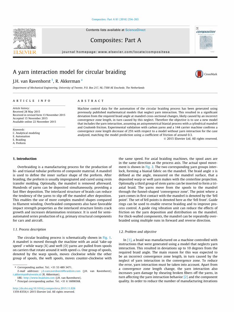
Force equilibrium equations can be applied to derive the posi-tions of the successive interlacement points on a yarn in the con-vergence zone, from the fell point with the prescribed fiberorientation up to the supply point. The yarn segments betweentwo interlacement points are described as two-force members,with Coulomb friction at the interlacements. Yarn compressiontowards the fell point is taken into account, including the resultingincrease in yarn thickness and its effect on the friction forces. The

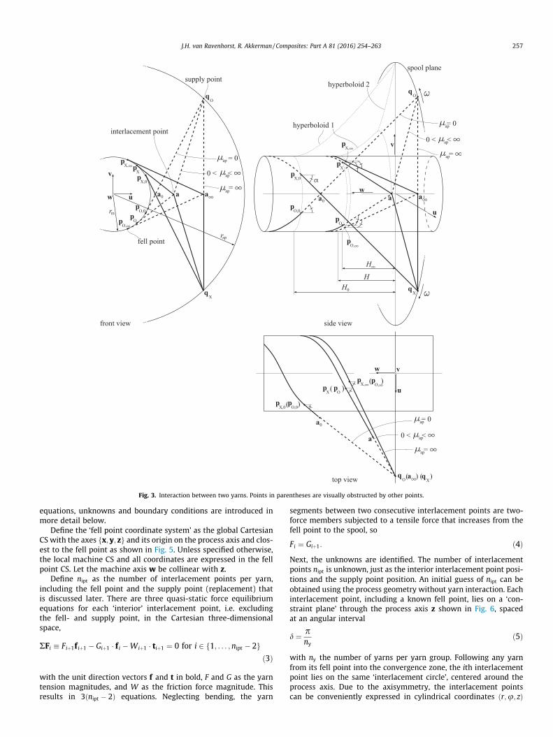
Fig. 3. Interaction between two yarns. Points in parentheses are visually obstructed by other points.

J.H. van Ravenhorst, R. Akkerman / Composites: Part A 81 (2016) 254–263 257

equations, unknowns and boundary conditions are introduced inmore detail below.

Define the ‘fell point coordinate system’ as the global CartesianCS with the axes fx; y; zg and its origin on the process axis and clos-est to the fell point as shown in Fig. 5. Unless specified otherwise,the local machine CS and all coordinates are expressed in the fellpoint CS. Let the machine axis w be collinear with z.

Define nipt as the number of interlacement points per yarn,including the fell point and the supply point (replacement) thatis discussed later. There are three quasi-static force equilibriumequations for each ‘interior’ interlacement point, i.e. excludingthe fell- and supply point, in the Cartesian three-dimensionalspace,

RFi � Fiþ1f iþ1 � Giþ1 � f i �Wiþ1 � tiþ1 ¼ 0 for i 2 f1; . . . ; nipt � 2gð3Þ

with the unit direction vectors f and t in bold, F and G as the yarntension magnitudes, and W as the friction force magnitude. Thisresults in 3ðnipt � 2Þ equations. Neglecting bending, the yarn

segments between two consecutive interlacement points are two-force members subjected to a tensile force that increases from thefell point to the spool, so

Fi ¼ Giþ1: ð4ÞNext, the unknowns are identified. The number of interlacementpoints nipt is unknown, just as the interior interlacement point posi-tions and the supply point position. An initial guess of nipt can beobtained using the process geometry without yarn interaction. Eachinterlacement point, including a known fell point, lies on a ‘con-straint plane’ through the process axis z shown in Fig. 6, spacedat an angular interval

d ¼ pny

ð5Þ

with ny the number of yarns per yarn group. Following any yarnfrom its fell point into the convergence zone, the ith interlacementpoint lies on the same ‘interlacement circle’, centered around theprocess axis. Due to the axisymmetry, the interlacement pointscan be conveniently expressed in cylindrical coordinates ðr;u; zÞ

Fig. 4. Instantaneous kinematics in the plane parallel to the machine v-axis, andthrough the coplanar points a; pO; pX; qO and qX.

258 J.H. van Ravenhorst, R. Akkerman / Composites: Part A 81 (2016) 254–263

shown in Figs. 5 and 6. Given a known fell point a0 of a yarn, previ-ously denoted by p in Fig. 3, the ith interlacement point on that yarnhas the angle

ui ¼ u0 þ signðxygrw � zÞi � d ð6Þ

where u0 corresponds to the fell point. The sign function is used toindicate that the sense depends on the combination of the signedyarn group dependent carrier rotation speed xygr and the machineorientation in the fell point CS, indicated by the dot productw � z. As

Fig. 5. Detail geometry of a yarn

a consequence, the only interlacement point degrees of freedom leftare r and z.

The boundary conditions to be prescribed are the fell point a0

and its yarn direction f0, corresponding to the prescribed braidangle. The yarn segment between a0 and a1 is constrained to bein direction f0 using the corresponding direction cosine,

Dcos � a1 � a0

jja1 � a0jj � f0 � 1 ¼ 0: ð7Þ

Generally, the supply point is not an interlacement point anddoes not lie on a constraint plane. For a valid solution, one ‘virtual’interlacement point must lie outside the creating circle radius rccas shown in Fig. 6. The supply point is the intersection betweenthe creating circle extrusion and the yarn polyline end segmentconnected to the virtual point. The virtual point is included innipt, replacing the actual supply point. The yarn tension magnitudemust be prescribed as a boundary condition at the virtual point.

The number of variables in r and z to be solved is 2ðnipt � 1Þ,excluding the known fell point and including the virtual interlace-ment point. This number is exceeded by the 3ðnipt � 2Þ force equi-librium Eq. (3), making the system of equations overdetermined.However, approximate solutions can be obtained using non-linear optimization techniques as shown in the next section. Inthe remainder of this section, the constituents of Eq. (3) arederived, mainly using Fig. 5.

Coulomb friction is used to obtain the friction force magnitude,

Wi ¼ lapNi ð8Þwith lap as the average apparent dynamic inter-yarn coefficient offriction and Ni as the local normal force magnitude, approximatedas shown in Fig. 7 by

Ni ¼ ðFi þ GiÞ sinðhiÞ ð9Þ

s in the convergence zone.

Fig. 6. Front view showing interlacement circles and interlacement point constraintplanes at intervals d. In this case, the number of interlacement points per yarn nipt is16.

Fig. 7. Simplified yarn interaction. Generally, g– 90� .

Fig. 8. Cross-section of the convergence zone, viewed perpendicularly to both thelocal yarn centerline direction and the local yarn thickness direction. From top tobottom: A ‘diamond braid’ having nfloat ¼ 1, and three ‘regular braids’ havingnfloat ¼ 2 with a decreasing yarn-to-yarn spacing, resulting in a yarn thicknessincrease that can occur when traveling to the fell point.

Fig. 9. Yarn width wy as a function of the available width wav and the initial yarn

J.H. van Ravenhorst, R. Akkerman / Composites: Part A 81 (2016) 254–263 259

assuming only a small rate of change of F; G and ‘crimp angle’ halong the yarn. As shown in Fig. 8, hi is approximated by

hi ¼arctan ty;i

pi

� �nfloat

ð10Þ

with

pi ¼ jjaiþ1 � aijj ð11Þ

as the ‘interlacement pitch’, nfloat as the constant braid ‘float length’(the number of ends) of either a plain weave (nfloat ¼ 1) or a2/2-twill (nfloat ¼ 2), and ty;i as the local yarn thickness,

ty;i ¼ Ay

wy;ið12Þ

with wy;i as the local yarn width and Ay as the constant yarn cross-sectional area,

Ay ¼ ql

v fqfð13Þ

with ql as the yarn linear density (kg/m), v f the yarn fiber volumefraction and qf the fiber density (kg/m3). Neglecting the yarnspreading and allowing the yarn to reduce in width without defor-mation resistance, the local yarn width wy;i in Eq. (12) is modeled asshown in Fig. 9 using

wy;i ¼wy;ini if wav;i P wy;ini;

wav;i if wav;i < wy;ini

�ð14Þ

with wy;ini as the initial yarn width on the spool andwav;i as the localavailable width, assuming only a small rate of change for wav.Between the ith and ðiþ 1Þth interlacement point,

wav;i ¼ 2di sinwi ð15Þusing the symbols in Fig. 5. To obtain the parameters di and wi, thefollowing parameters are required. The interlacement circle tangentt points in the yarn rotation direction when traveled from fell tospool, corresponding to the relative yarn sliding direction asdescribed in Section 2.2,

ti ¼ signðxygrÞ w� ai

jjw� aijj : ð16Þ

Define si as the local unit direction vector from ai to the adjacentinterlacement point on the same interlacement circle, having thesame sense as ti. Express T as the constant transformation matrixthat rotates t around w by an angle d to yield s,

T ¼c �s 0s c 00 0 1

264

375: ð17Þ

with the coefficients c ¼ cos½signðxygrw � zÞd� ands ¼ sin½signðxygrw � zÞd�. Nowsi ¼ Tti: ð18ÞIn Eq. (15), the angle wi is the ‘pseudo-braid angle complement’,

wi ¼ arccosðf i � siÞ: ð19Þand di is half the local Euclidean distance between two adjacentinterlacement points on the same interlacement circle,

di ¼ ri sin d ð20Þwith d from Eq. (5) and radius ri as the distance between ai and theprocess axis,

ri ¼ jjai � ðai �wÞwjj: ð21Þ

width wy;ini.

260 J.H. van Ravenhorst, R. Akkerman / Composites: Part A 81 (2016) 254–263

2.4. Implementation

An implementation involving non-linear optimization tech-niques is presented, followed by a ‘frontal approach’. No genericconcise analytical expression of the convergence zone length as afunction of the input parameters was found. Instead, onlycase-specific numerical simulations can be performed using theproposed approaches.

2.4.1. Non-linear optimization approachThe problem was solved using Matlab’s [12] ‘fsolve’ command.

This command requires a function f as input and solves f ðxÞ ¼ 0without requiring any derivative of f as input. Here,

f ðxÞ ¼ y ð22Þwith the unknown cylindrical coordinates of the interlacementpoints as input,

x ¼ r1 r2 . . . rnipt�2 rnipt�1

z1 z2 . . . znipt�2 znipt�1

" #: ð23Þ

Not shown here are the constant process parameter inputslisted in Table 1. The outputs are the resultant force residuals fromEq. (3) in Cartesian coordinates and the residual direction cosinefrom Eq. (7),

y ¼ RF1 RF2 . . . RFnipt�3 RFnipt�2 Dcos� �

: ð24ÞThe function f first transforms the input coordinates to Carte-

sian. Next, for each interlacement point and yarn segment, thegeometry is evaluated using Eqs. (10)–(21). Finally, the terms ofEq. (24) are evaluated. Further implementation details of f arebeyond the scope of this work. The ‘Trust-Region-Reflective’ solverwas assigned to fsolve for obtaining a solution to Eq. (22). The sol-ver performs a non-linear optimization (NLO), providing the namefor this approach. An NLO generally has Oðn3Þ time complexity,where n is the number of unknowns. It can have zero, one or mul-tiple solutions, depending on the applied friction model and theboundary condition magnitudes. The emerging solution dependson the initial guess of the interlacement point positions. Strategiesfor finding the correct solution are beyond the scope of this work.

2.4.2. Frontal approachAn approximate solution can also be obtained using a computa-

tionally faster ‘frontal sweep’ for a single interlacement point at atime, starting at the fell point and progressing through the conver-gence zone until a virtual interlacement point is found outside of

Table 1Constant input parameters of the problem, matching the experimental values.

Parameter Value

Yarn fiber density ql 1780 kg/m3

Yarn linear density qf 830 � 10�6 kg/mYarn fiber volume fraction v f 0.7Yarn initial width wy;ini 4 � 10�3 m

Spool plane radius rsp 1.382 mNumber of yarns per group ny 72Number of floats nfloat 2Spool tension Fsp 4.7 NApparent average dynamic coefficient of friction lap 0.2

Machine axis w (0, 0, �1) mMandrel radius rm 75 � 10�3 mFell point coordinates a0 (rm, 0, 0) mBraid angle a 60�Fell point tangent f0 (0, sina; cosa) mYarn group (X or O) X

the creating circle radius rcc. The supply point is obtained as theintersection between the last yarn segment and the surface ofthe creating circle extrusion. The same boundary conditions fromthe NLO approach apply. As an initial guess, the tension magnitudeF0 ¼ Fsp is used at the known fell point a0 with the known fiberdirection f0. For the approximation of the normal force N, onlythe tension at the fell point side is used, and the crimp angle h ofthe previous point is used, assuming only a gradual change,replacing Eq. (9),

Niþ1 ¼ 2Fi sin hið Þ ð25ÞSimilarly, instead of calculating the interlacement pitch pi using

two interlacement points in Eq. (11), using Fig. 5,

pi ¼di

coswi: ð26Þ

From the fell point to the spool, the next interlacement point isobtained by

aiþ1 ¼ ai þ pifi: ð27Þeliminating Eq. (7). The evaluation order of the equations at eachinterlacement point is shown in Fig. 10 and is traceable usingFig. 5. The implementation of this evaluation sequence has OðnÞtime complexity, where n ¼ nipt, and therefore offers a dramaticcomputation time reduction compared to the NLO, although

Fig. 10. Simplified flow charts summarizing function evaluations for each inter-lacement point in the frontal approach.

J.H. van Ravenhorst, R. Akkerman / Composites: Part A 81 (2016) 254–263 261

obviously slower than the Oð1Þ time complexity without yarn inter-action. There is no need for an initial guess of the interlacementpoint coordinates and they inherently coincide with the constraintplanes. If Coulomb friction is used, the friction force W scales withthe same factor as the tension force F. As a consequence, at eachinterlacement point the yarn kink angle is independent of the ten-sion magnitude, and, in turn, the yarn geometry and convergencezone length are independent of the spool tension. Given the solu-tion geometry, the corresponding tension distribution can be eval-uated as a post-processing step.

3. Numerical case study

Both approaches are compared to assess if the faster frontalapproximation yields a solution that is close enough to the moregeneric NLO approach.

A centered cylindrical mandrel is overbraided without the useof guide rings. The used parameter values are listed in Table 1and correspond as good as practically possible to the physicallyequivalent experiment described in Section 4. The expected coeffi-cient of friction of approximately 0.2 is based on perpendiculartow-to-tow friction measurements from [8,9] and is primarily usedfor the numerical comparison. The result is a non-jamming braidand a full mandrel surface coverage, which is usually desired.Figs. 11 and 12 represent the positions of the successive interlace-ment points, which show that for this case the systematic error ofthe frontal approach is negligible compared to that of the NLOapproach and that the latter appears to yield the correct solution.

A parametric study showed a substantial convergence zonelength decrease of 50 mm per 0.1 difference in lap. Variation ofthe other parameters resulted in relatively small changes.

4. Experiment

The experimental setup consists of a hot-wire cut styrofoamcylindrical mandrel with its axis coinciding with the braiding

10

100

1000

10000

0 10 20 30 40 50 60 70 80 90 100

r (m

m)

ϕ (deg)

frontalroot finding

Fig. 11. Interlacement point r-parameter values at their constraint plane angles.The angular increment of u between two interlacement points is 2:5� .

1

10

100

1000

10000

0 10 20 30 40 50 60 70 80 90 100

z (m

m)

ϕ (deg)

frontalroot finding

Fig. 12. Interlacement point z-parameter values at their constraint plane angles.The angular increment of u between two interlacement points is 2:5� .

machine axis. The mandrel is clamped on a aluminum tube havinga bending stiffness high enough to limit the gravity-induceddeflection below a millimeter, asserting the axisymmetry assump-tion. A Eurocarbon 144 carrier machine without guide rings asshown in Fig. 13 was used and a single yarn material, Teijin TohoTenax IMS65 E23 24k carbon yarn was used for both yarn groups.The corresponding values are listed in Table 1.

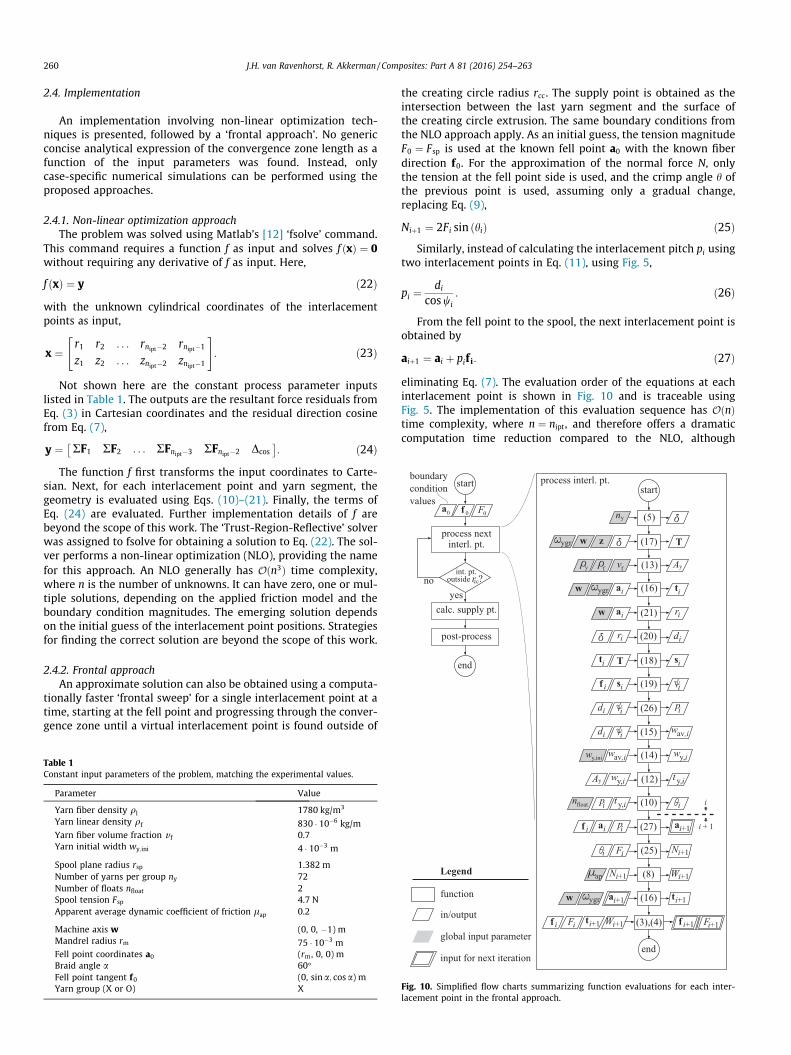
It was made sure that the process was in steady state to avoidnon-prescribed transient braid angles [13]. For this purpose, a dis-tance of 500 mmwas overbraided and the braid angle was assertedto be 60 degrees using a goniometer. It is noted that immediatelyafter stopping the machine, the yarns show a viscous-like yarnmotion which is not modeled. Fiber breakage and entanglementsoccurred at the scale ranging from single fibers to yarns, some-times leading to situations as shown in Fig. 14, significantly affect-ing the yarn geometry in the convergence zone. Besides theentanglement that can be visualized in photographs, the entireconvergence zone is permanently covered with a very fine webof detached fibers. Close-range photogrammetry was used to tracethe 3D trajectory of yarns. During this measurement, the yarnswere not touched. For this purpose, a tubular frame was builtand put around the mandrel to hold coded targets as referencepoints for the measurement. Using Photomodeler [14], a genericphotogrammetry software, ten warp yarn curves were extractedas piecewise linear curves with a negligible measurement error.Close to the fell points, individual yarns segments could not beproperly distinguished and were not processed further.

5. Results and discussion

The yarns were modeled using the frontal approach for a rangeof friction coefficients, from l ¼ 0 to 3 and transformed to emergefrom a single spool as shown in Fig. 15. Analogously, the experi-mentally obtained yarn polylines were added to the same viewfor comparison. In the model and experiment, the yarn curves inthe convergence zone are not planar. The yarn curvature is rela-tively large near the fell front and rapidly decreases towards thespools. The experimental yarns are closest to the modeled yarnwith lap ¼ 0:3. This value is higher than the value of 0.2 used in

Fig. 13. Experimental setup at Eurocarbon. Top right: Fell front with pairwise yarnclustering. The dashed region is magnified in Fig. 14.

to fell front

to spools

Fig. 14. A magnification of the region indicated in Fig. 13, showing a cluster ofbroken fibers, emphasized by the dashed line, and the effect after entanglementwith yarns, causing the yarns to kink as indicated by the white arrows. The yarnmoving direction is indicated by the black arrows.

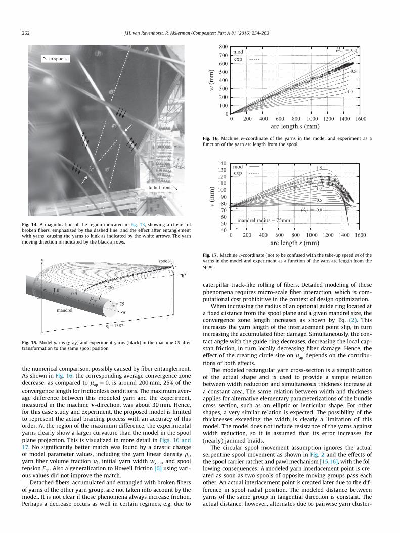
Fig. 15. Model yarns (gray) and experiment yarns (black) in the machine CS aftertransformation to the same spool position.

Fig. 16. Machine w-coordinate of the yarns in the model and experiment as afunction of the yarn arc length from the spool.

Fig. 17. Machine v-coordinate (not to be confused with the take-up speed v) of theyarns in the model and experiment as a function of the yarn arc length from thespool.

262 J.H. van Ravenhorst, R. Akkerman / Composites: Part A 81 (2016) 254–263

the numerical comparison, possibly caused by fiber entanglement.As shown in Fig. 16, the corresponding average convergence zonedecrease, as compared to lap ¼ 0, is around 200 mm, 25% of theconvergence length for frictionless conditions. The maximum aver-age difference between this modeled yarn and the experiment,measured in the machine v-direction, was about 30 mm. Hence,for this case study and experiment, the proposed model is limitedto represent the actual braiding process with an accuracy of thisorder. At the region of the maximum difference, the experimentalyarns clearly show a larger curvature than the model in the spoolplane projection. This is visualized in more detail in Figs. 16 and17. No significantly better match was found by a drastic changeof model parameter values, including the yarn linear density ql,yarn fiber volume fraction v f , initial yarn width wy;ini, and spooltension Fsp. Also a generalization to Howell friction [6] using vari-ous values did not improve the match.

Detached fibers, accumulated and entangled with broken fibersof yarns of the other yarn group, are not taken into account by themodel. It is not clear if these phenomena always increase friction.Perhaps a decrease occurs as well in certain regimes, e.g. due to

caterpillar track-like rolling of fibers. Detailed modeling of thesephenomena requires micro-scale fiber interaction, which is com-putational cost prohibitive in the context of design optimization.

When increasing the radius of an optional guide ring located ata fixed distance from the spool plane and a given mandrel size, theconvergence zone length increases as shown by Eq. (2). Thisincreases the yarn length of the interlacement point slip, in turnincreasing the accumulated fiber damage. Simultaneously, the con-tact angle with the guide ring decreases, decreasing the local cap-stan friction, in turn locally decreasing fiber damage. Hence, theeffect of the creating circle size on lap depends on the contribu-tions of both effects.

The modeled rectangular yarn cross-section is a simplificationof the actual shape and is used to provide a simple relationbetween width reduction and simultaneous thickness increase ata constant area. The same relation between width and thicknessapplies for alternative elementary parameterizations of the bundlecross section, such as an elliptic or lenticular shape. For othershapes, a very similar relation is expected. The possibility of thethicknesses exceeding the width is clearly a limitation of thismodel. The model does not include resistance of the yarns againstwidth reduction, so it is assumed that its error increases for(nearly) jammed braids.

The circular spool movement assumption ignores the actualserpentine spool movement as shown in Fig. 2 and the effects ofthe spool carrier ratchet and pawl mechanism [15,16], with the fol-lowing consequences: A modeled yarn interlacement point is cre-ated as soon as two spools of opposite moving groups pass eachother. An actual interlacement point is created later due to the dif-ference in spool radial position. The modeled distance betweenyarns of the same group in tangential direction is constant. Theactual distance, however, alternates due to pairwise yarn cluster-

J.H. van Ravenhorst, R. Akkerman / Composites: Part A 81 (2016) 254–263 263

ing as shown in Fig. 13, caused by violating axisymmetry. Thisleads to the two distinct groups (each containing warp and weftyarns) of experimental data points in Figs. 16 and 17. All modeledyarns are subjected to the same constant tension. The actual ten-sion fluctuates, optionally affected by empty carriers. For the ficti-tious case of a machine radius that is much larger than the mandrelradius and the neglect of ratcheting, the tension waveform wouldbe similar to the spool amplitude waveform. For radial braidingmachines, this geometrical fluctuation is almost eliminated. Conse-quently, the yarn interlacement geometry shown in Fig. 8 is a fairlycoarse approximation.

Finally, the assumed coincidence of the fell point and an inter-lacement point is generally incorrect. However, in the commoncase of full mandrel coverage, adjacent yarns of a single groupare approximately in lateral contact with each other, reducingthe error to the order of one yarn width.

6. Conclusions

A yarn interaction model was developed for the axisymmetricalbiaxial braiding process, implemented with non-linear optimiza-tion techniques and a computationally faster frontal approach.Comparison of the two approaches showed no significant differ-ence in the resulting yarn geometry. A parametric study usingthe frontal approach showed that the result is mainly affected bythe coefficient of friction for the case under consideration. A valida-tion with a physical experiment using carbon yarns shows that amodeled coefficient of friction value around 0.3 provides the clos-est match between model and experiment. For this value, both themodel and the experiment show a significant convergence zonedecrease around 25% with respect to the frictionless model forthe particular case studied here. This confirms that yarn interactiondoes significantly affect the convergence zone length. Hence, whengenerating machine control data for accurate results, neglect ofthis change in convergence zone length can cause significant braidangle errors. The main limitations of this model and many otherbraiding simulation models including those using a finite elementapproach are that they do not capture the effect of broken,detached and entangled fibers with a large effect on the inter-yarn forces. In addition, the model presented here neglects thenon-axisymmetrical features, especially tension fluctuation andpairwise yarn clustering.

7. Recommendations

More experiments are needed to evaluate if the model resultsremain consistent with the experiments. To remove the effect offiber damage, a different, possibly tape-like yarn can be chosen.However, the bending stiffness should remain as low as possiblein order to match the model, or the model should be extended toinclude bending stiffness. The latter would advocate a finite ele-ment approach, although this still neglects the effects of fiberdamage.

Benchmarking of the frontal approach and kinematic models ingeneral against finite element approaches can be performed toevaluate the trade-off between accuracy and speed.

For larger braiding machines, gravity effects may become morepronounced, varying the resulting braid angle as a function of thecircumferential position. Again, a finite element approach is pre-ferred for this purpose.

The model can be integrated into kinematic braiding simulationsoftware like Braidsim [17] and can be used to generate take-upspeed profiles for the production of braids with braid angles thatsatisfy the tolerances better than the results from models neglect-ing it. To include guide rings, the frontal approach can be extended.

For more generic process configurations including deviationsfrom axisymmetry and the addition of stem yarns, differentapproaches like finite elements or kinematics without yarn inter-action are required. However, in the component design phase gen-erally the former is too slow and the latter is too inaccurate.Therefore current research focuses on the generalization of thepresented yarn interaction model to work with arbitrary mandrelcross-sections and further research in this area is required.

Acknowledgement

The support of Eurocarbon B.V. is gratefully acknowledged.

References

[1] van Ravenhorst JH, Akkerman R. Circular braiding take-up speed generationusing inverse kinematics. Compos Part A: Appl Sci Manuf 2014;64:147–58.

[2] Ebel C, Brand M, Drechsler K. Effects of fiber damage on the efficiency of thebraiding process. In: TexComp-11 conference. 16–20 September 2013, Leuven;2013.

[3] Du GW, Popper P. Analysis of a circular braiding process for complex shapes. JText Inst 1994;85:316–37.

[4] Zhang Q, Beale D, Broughton RM. Analysis of circular braiding process, Part 1:theoretical investigation of kinematics of the circular braiding process. J ManufSci Eng 1999;121:345–50.

[5] Zhang Q, Beale D, Broughton RM. Analysis of circular braiding process, Part 2:mechanics analysis of the circular braiding process and experiment. J ManufSci Eng 1999;121:351–9.

[6] Howell HG, Mazur J. Amonton’s law and fiber friction. J Text Inst 1953;44(2):T59–69.

[7] Mazzawi A. The steady state and transient behaviour of 2D braiding. Ph.D.thesis. University of Ottawa; 2001.

[8] Pickett A, Erber A, von Reden T, Drechsler K. Comparison of analytical and finiteelement simulation of 2D braiding. Plast Rubber Compos 2009;38:387–95.

[9] Cornelissen B, Rietman AD, Akkerman R. Frictional behaviour of highperformance fibrous tows: friction experiments. Compos Part A: Appl SciManuf 2013;44:95–104.

[10] Brunnschweiler D. Braids and braiding. J Text Inst Proc 1953;44(9):666–86.[11] Ko FK, Pastore CM, Head AA. Handbook of industrial braiding. Atkins and

Pearce; 1989.[12] www.mathworks.com; 2015a.[13] Nishimoto H, Ohtani A, Nakai A, Hamada H. Prediction method for temporal

change in fiber orientation on cylindrical braided preforms. Text Res J 2010;80(9):814–21.

[14] www.photomodeler.com; 2015b.[15] Ma G, Branscomb DJ, Beale DG. Modeling of the tensioning system on a

braiding machine carrier. Mech Mach Theory 2012;47(0):46–61.[16] Rosenbaum JU. Flechten: rationelle Fertigung faserverstärkter

Kunststoffbauteile. Verl. TÜV Rheinland; 1991. ISBN 9783885859796.[17] www.braidsim.com; 2015c.