arX

iv:a

stro

-ph/

0105

231v

1 1

4 M

ay 2

001

Composite Quasar Spectra From the Sloan Digital Sky Survey1

Daniel E. Vanden Berk2, Gordon T. Richards3, Amanda Bauer4, Michael A. Strauss5, Donald P.

Schneider3, Timothy M. Heckman6, Donald G. York7,8, Patrick B. Hall5, Xiaohui Fan5,9, G. R.

Knapp5, Scott F. Anderson10, James Annis2, Neta A. Bahcall5, Mariangela Bernardi7, John W.

Briggs7, J. Brinkmann11, Robert Brunner12, Scott Burles2, Larry Carey10, Francisco J.

Castander7,13, A. J. Connolly14, J. H. Crocker6, Istvan Csabai6,15, Mamoru Doi16, Douglas

Finkbeiner17, Scott Friedman6, Joshua A. Frieman2,7, Masataka Fukugita18, James E. Gunn5, G.

S. Hennessy19, Zeljko Ivezic5 , Stephen Kent2,7, Peter Z. Kunszt6, D.Q. Lamb7, R. French Leger10,

Daniel C. Long11, Jon Loveday20, Robert H. Lupton5, Avery Meiksin21, Aronne Merelli12,22,

Jeffrey A. Munn23, Heidi Jo Newberg24, Matt Newcomb22, R. C. Nichol22, Russell Owen10,

Jeffrey R. Pier23, Adrian Pope6,22, Constance M. Rockosi7, David J. Schlegel5, Walter A.

Siegmund10, Stephen Smee6,25, Yehuda Snir22, Chris Stoughton2, Christopher Stubbs10, Mark

SubbaRao7, Alexander S. Szalay6, Gyula P. Szokoly6, Christy Tremonti6, Alan Uomoto6, Patrick

Waddell10, Brian Yanny2, Wei Zheng6

– 2 –

ABSTRACT

We have created a variety of composite quasar spectra using a homogeneous data

set of over 2200 spectra from the Sloan Digital Sky Survey (SDSS). The quasar sample

spans a redshift range of 0.044 ≤ z ≤ 4.789, and an absolute r′ magnitude range of

−18.0 to −26.5. The input spectra cover an observed wavelength range of 3800−9200A

1Based on observations obtained with the Sloan Digital Sky Survey, which is owned and operated by the Astro-

physical Research Consortium.

2Fermi National Accelerator Laboratory, P.O. Box 500, Batavia, IL 60510

3Department of Astronomy and Astrophysics, The Pennsylvania State University, University Park, PA 16802

4Department of Physics, University of Cincinnati, 400 Physics Bldg., Cincinnati, OH 45221

5Princeton University Observatory, Princeton, NJ 08544

6Department of Physics and Astronomy, The Johns Hopkins University, 3701 San Martin Drive, Baltimore, MD

21218

7The University of Chicago, Department of Astronomy and Astrophysics, 5640 S. Ellis Ave., Chicago, IL 60637

8The University of Chicago, Enrico Fermi Institute, 5640 S. Ellis Ave., Chicago, IL 60637

9Institute for Advanced Study, Olden Lane, Princeton, NJ 08540

10University of Washington, Department of Astronomy, Box 351580, Seattle, WA 98195

11Apache Point Observatory, P.O. Box 59, Sunspot, NM 88349-0059

12Department of Astronomy, California Institute of Technology, Pasadena, CA 91125

13Observatoire Midi Pyrenees, 14 ave Edouard Belin, Toulouse, F-31400, France

14Department of Physics and Astronomy, University of Pittsburgh, Pittsburgh, PA 15260

15Department of Physics of Complex Systems, Eotvos University, Pazmany Peter setany 1

16Department of Astronomy and Research Center for the Early Universe, School of Science, University of Tokyo,

Hongo, Bunkyo, Tokyo, 113-0033, Japan

17University of California at Berkeley, Departments of Physics and Astronomy, 601 Campbell Hall, Berkeley, CA

94720

18University of Tokyo, Institute for Cosmic Ray Reserach, Kashiwa, 2778582, Japan

19U.S. Naval Observatory, 3450 Massachusetts Ave., NW, Washington, DC 20392-5420

20Astronomy Centre, University of Sussex, Falmer, Brighton BN1 9QJ, United Kingdom

21Royal Observatory, Edinburgh, EH9 3HJ, United Kingdom

22Dept. of Physics, Carnegie Mellon University, 5000 Forbes Ave., Pittsburgh, PA-15232

23U.S. Naval Observatory, Flagstaff Station, P.O. Box 1149, Flagstaff, AZ 86002-1149

24Physics Department, Rensselaer Polytechnic Institute, SC1C25, Troy, NY 12180

25Department of Astronomy, University of Maryland, College Park, MD 20742-2421

– 3 –

at a resolution of 1800. The median composite covers a rest wavelength range from

800 − 8555 A, and reaches a peak signal-to-noise ratio of over 300 per 1 A resolution

element in the rest frame. We have identified over 80 emission line features in the

spectrum. Emission line shifts relative to nominal laboratory wavelengths are seen for

many of the ionic species. Peak shifts of the broad permitted and semi-forbidden lines

are strongly correlated with ionization energy, as previously suggested, but we find that

the narrow forbidden lines are also shifted by amounts which are strongly correlated

with ionization energy. The magnitude of the forbidden line shifts is . 100 km s−1,

compared to shifts of up to 550 kms−1 for some of the permitted and semi-forbidden

lines. At wavelengths longer than the Lyα emission, the continuum of the geometric

mean composite is well-fit by two power-laws, with a break at ≈ 5000 A. The frequency

power law index, αν , is −0.44 from ≈ 1300 − 5000 A, and −2.45 redward of ≈ 5000 A.

The abrupt change in slope can be accounted for partly by host galaxy contamination

at low redshift. Stellar absorption lines, including higher-order Balmer lines, seen in the

composites suggest that young or intermediate age stars make a significant contribution

to the light of the host galaxies. Most of the spectrum is populated by blended emission

lines, especially in the range 1500 − 3500A, which can make the estimation of quasar

continua highly uncertain unless large ranges in wavelength are observed. An electronic

table of the median quasar template is available.

Subject headings: quasars: emission lines — quasars:general

1. Introduction

Most quasar spectra from ultraviolet to optical wavelengths can be characterized by a fea-

tureless continuum and a series of mostly broad emission line features; compared with galaxies or

stars, these spectra are remarkably similar from one quasar to another. The first three principal

components spectra account for about 75% of the intrinsic quasar variance (Francis, Hewett, Foltz

& Chaffee 1992). Subtle global spectral properties can be studied by combining large numbers of

quasar spectra into composites. The most detailed composites (Francis et al. 1991; Zheng et al.

1997; Brotherton et al. 2000) use hundreds of moderate resolution spectra, and typically cover a

few thousand A in the quasar rest frame. These high signal-to-noise ratio (S/N) spectra reveal

variations from a single power law in the general continuum shape, and weak emission features that

are rarely detectable in individual quasar spectra.

The Sloan Digital Sky Survey (York et al. 2000, SDSS) already contains spectra for over 2500

quasars as of June 2000, and by survey end will include on the order of 105 quasar spectra. The

identification and basic measurement of this sample will be done using an automated pipeline,

part of which uses templates for object classification and redshift determination. As one of the

first uses of the initial set of spectra, we have created a composite quasar spectrum for use as a

– 4 –

template. The large number of spectra, their wavelength coverage, relatively high resolution, and

high signal-to-noise ratio, make the current SDSS sample ideal for the creation of composite quasar

spectra. The resulting composite spectrum covers a vacuum rest wavelength range of 800−8555 A.

The peak S/N per 1 A resolution element is over 300 near 2800A – several times higher than the

previous best ultraviolet/optical composites (e.g. Francis et al. 1991; Zheng et al. 1997; Brotherton

et al. 2000).

In addition to serving as a cross-correlation template, the composite is useful for the pre-

cise measurement of emission line shifts relative to nominal laboratory wavelengths, calculation of

quasar colors for improved candidate selection and photometric redshift estimates, the calculation

of K-corrections used in evaluating the quasar luminosity function, and for the estimation of the

backlighting flux density continuum for measurements of quasar absorption line systems. Compos-

ites can also be made from sub-samples of the input spectra chosen according to quasar properties

such as luminosity, redshift, and radio loudness. The dependence of global spectral characteristics

on various quasar properties will be the subject of a future paper (Vanden Berk et al. 2001). Here

we concentrate on the continuum and emission line properties of the global composite. We describe

the SDSS quasar sample in § 2, and the method used to generate the composite spectra in § 3.

The continuum and emission line features are measured and discussed in §§ 4 and 5. Wavelengths

throughout the paper are vacuum values, except when using the common notation for line identifi-

cation (truncated air values for wavelengths greater than 3000A, and truncated vacuum values for

wavelengths less than 3000A). We use the following values for cosmological parameters throughout

the paper: H0 = 100 km s−1, Ωm = 1.0, ΩΛ = 0, (q0 = 0.5).

2. The SDSS Quasar Sample

The spectra were obtained as part of the commissioning phase of the Sloan Digital Sky Survey.

Details of the quasar candidate target selection and spectroscopic data reduction will be given in

future papers (Richards et al. 2001b; Newberg et al. 2001; Frieman et al. 2001). The process is

summarized here. Quasar candidates are selected in the color space of the SDSS u′g′r′i′z′ filter

system (Fukugita et al. 1996), from objects found in imaging scans with the SDSS 2.5m telescope

and survey camera (Gunn et al. 1998). The effective central wavelengths of the filters for a power-law

spectrum with a frequency index of α = −0.5, are approximately 3560, 4680, 6175, 7495, and 8875A

for u′g′r′i′z′ respectively. Quasar candidates are well-separated from the stellar locus in color

space, and the filter system allows the discovery of quasars over the full range of redshifts from

z = 0 to z ≈ 7. The locations of known quasars in the SDSS color space as a function of redshift

are shown by Fan et al. (1999, 2000, 2001); Newberg et al. (1999); Schneider et al. (2001) and

especially Richards et al. (2001a) who plot the locations of over 2600 quasars for which there is

SDSS photometry. Quasar candidates are selected to i′ ≈ 19 in the low-redshift (z . 2.5) regions of

color space, and no discrimination is made against extended objects in those regions. High-redshift

quasar candidates are selected to i′ ≈ 20. Objects are also selected as quasar candidates if they

– 5 –

are point sources with i′ ≤ 19 and match objects in the VLA FIRST radio source catalog (Becker,

White & Helfand 1995). Thus, quasars in the SDSS are selected both by optical and radio criteria.

These data were taken while the hardware, and in particular the target selection software, was

being commissioned. Therefore, the selection criteria for quasars has evolved somewhat over the

course of these observations, and will not exactly match the final algorithm discussed in Richards

et al. (2001b). Because of the changing quasar selection criteria and the loose definition of ’quasar’,

discretion should be exercised when using the global composite spectra generated from this quasar

sample as templates for quasars in other surveys, or subsets of the SDSS quasar sample.

The candidates were observed using the 2.5m SDSS telescope (Siegmund et al. 2001) at Apache

Point Observatory, and a pair of double fiber-fed spectrographs (Uomoto et al. 2001). Targeted

objects are grouped into 3 degree diameter “plates”, each of which holds 640 optical fibers. The

fibers subtend 3′′ on the sky and their positions on the plates correspond to the coordinates of

candidate objects, sky positions, and calibration stars. Approximately 100 fibers per plate are

allocated to quasar candidates. At least three 15 minute exposures are taken per plate. So far,

spectra have been taken mainly along a 2.5 degree wide strip centered on the Celestial Equator, with

a smaller fraction at other declinations. The spectra in this study were grouped on 66 plates which

overlap somewhat to cover approximately 320 square degrees of sky covered by the imaging survey.

The plates were observed from October, 1999 to June, 2000. The raw spectra were reduced with the

SDSS spectroscopic pipeline (Frieman et al. 2001), which produces wavelength- and flux-calibrated

spectra that cover an observed wavelength range from 3800 − 9200A at a spectral resolution of

approximately 1850 blueward of 6000A, and 2200 redward of 6000A. These spectra and more will

be made publicly available – in electronic form – in June 2001 as part of the SDSS Early Data

Release (Stoughton et al. 2001).

The flux calibration is only approximate at this time, and a point which deserves elaboration

since it is the most important source of uncertainty in the continuum shapes of the spectra. Light

losses from differential refraction during the observations are minimized by tracking guide stars

through a g′ filter – the bluest filter within the spectral range. Several F subdwarf stars are selected

for observation (simultaneously with the targeted objects) on each plate. One of these – usually the

bluest one – is selected, typed, and used to define the response function. This process also largely

corrects for Galactic extinction, since the distances to the F subdwarfs employed are typically

greater than 2.5kpc, and all of the survey area is at high Galactic latitude. Uncertainties can arise

in the spectral typing of the star, and from any variation in response across a plate. A check on the

accuracy of the flux calibration is made for each plate by convolving the calibrated spectra with

the filter transmission functions of the g′, r′, and i′ bands, and comparing the result to magnitudes

derived from the imaging data using an aperture the same diameter as the spectroscopic fibers. For a

sample of about 2300 SDSS quasar spectra, the median color difference between the photometric and

spectral measurements, after correcting the photometric values for Galactic extinction (Schlegel,

Finkbeiner, & Davis 1998), was found to be ∆(g′ − r′) ≈ 0.01 and ∆(r′ − i′) ≈ 0.04. This means

that the spectra tend to be slightly bluer than expectations from photometry. For a pure power-law

– 6 –

spectrum with true frequency index of αν = −0.5, which is often used to approximate quasars, the

difference in both colors would result in a measured index which is systematically greater (bluer)

by about 0.1. Quasar spectra are not pure power-laws, and the color differences are well within

the intrinsic scatter of quasars at all redshifts (Richards et al. 2001a). Also, the SDSS photometric

calibration is not yet finalized, and the shapes of the filter transmission curves are still somewhat

uncertain, both of which could contribute to the spectroscopic vs. photometric color differences.

The colors of the combined spectra agree well with the color-redshift relationships found by Richards

et al. (2001a), (see §§ 4.2,5) which also leads us to believe that the flux calibrations are reasonably

good. However, we caution that the results here on the combined continuum shape cannot be

considered final until the SDSS spectroscopic calibration is verified.

Quasars were identified from their spectra and approximate redshift measurements were made

by manual inspection.26 We define quasar to mean any extra-galactic object with at least one broad

emission line, and that is dominated by a non-stellar continuum. This includes Seyfert galaxies

as well as quasars, and we do not make a distinction between them. Spectra were selected if the

rest-frame FWHM of the strong permitted lines, such as C iv , Mg ii , and the Balmer lines, were

greater than about 500 km s−1. In most cases those line widths well exceeded 1000 km s−1. Since

we require only one broad emission line, some objects which may otherwise be classified as “Type

2” AGN (those with predominantly narrow emission lines) are also included in the quasar sample.

Spectra with continua dominated by stellar features, such as unambiguous Ca H and K lines, or the

4308A G-band, were rejected. This definition is free from traditional luminosity or morphology-

based criteria, and is also intended to avoid introducing a significant spectral component from the

host galaxies (see § 5). Spectra with broad absorption line features (BAL quasars), which comprise

about 4% of the initial sample, were removed from the input list. We are studying BAL quasars in

the SDSS sample intensively, and initial results are forthcoming (Menou et al. 2001, e.g.); the focus

of the present paper is on the intrinsic continua of quasars, and BAL features can heavily obscure

the continua. Other spectra with spurious artifacts introduced either during the observations or

by the data reduction process (about 10% of the initial sample) were removed from the input

list.27 Spectra obtained as part of SDSS follow-up observations on other telescopes, such as the

high-redshift samples of Fan et al. (1999, 2000, 2001), Schneider et al. (2000, 2001), and Zheng

et al. (2000) were not included. Figure 1 shows the redshift distribution of the quasars used in the

composite, and the absolute r′ magnitudes vs. redshift. Discontinuities in the selection function for

the quasars, such as the fainter magnitude limit for high-redshift candidates, are evident in Figure 1.

The final list of spectra contains 2204 quasars spanning a redshift range of 0.044 ≤ z ≤ 4.789, with

a median quasar redshift of z = 1.253. The vast majority of the magnitudes lie in the range

17.5 < r′ < 20.5.

26Refined redshift measurements were made later as described in § 3.

27These artifacts are due to the inevitable problems of commissioning both the software and hardware, and the

problem rate is now negligible.

– 7 –

3. Generating the Composites

The steps required to generate a composite quasar spectrum involve selecting the input spectra,

determining accurate redshifts, rebinning the spectra to the rest frame, scaling or normalizing the

spectra, and stacking the spectra into the final composite. Each of these steps can have many

variations, and their effect on the resulting spectrum can be significant (see Francis et al. (1991)

for a discussion of some of these effects). The selection of the input spectra was described in the

previous section, and here we detail the remaining steps.

The appropriate statistical methods used to combine the spectra depend upon the spectral

quantities of interest. We are interested in both the large-scale continuum shape and the emission

line features of the combined quasars. We have used combining techniques to generate two compos-

ite spectra: 1) the median spectrum which preserves the relative fluxes of the emission features; and

2) the geometric mean spectrum which preserves the global continuum shape. We have used the

geometric mean because quasar continua are often approximated by power-laws, and the median

(or arithmetic mean) of a sample of power-law spectra will not in general result in a power-law

with the mean index. The geometric mean is defined as, 〈fλ〉gm = (∏n

i=1 fλ,i)1/n, where fλ,i is

the flux density of spectrum number i in the bin centered on wavelength λ, and n is the number

of spectra contributing to the bin. Assuming a power-law form for the continuum flux density,

fλ ∝ λ−(αν+2), it is easily shown that 〈fλ〉gm ∝ λ−(〈αν 〉+2), where 〈αν〉 is the (arithmetic) mean

value of the frequency power-law index. (The wavelength index, αλ, and the frequency index, αν ,

are related by αλ = −(αν + 2).)

The rest positions of emission lines in quasar spectra, especially the high-ionization broad lines,

are known to vary from their nominal laboratory wavelengths (Gaskell 1982; Wilkes 1986; Espey

et al. 1989; Zheng & Sulentic 1990; Corbin 1990; Weymann, Morris, Foltz & Hewett 1991; Tytler

& Fan 1992; Brotherton, Wills, Steidel & Sargent 1994; Laor et al. 1995; McIntosh, Rix, Rieke &

Foltz 1999), so the adopted redshifts of quasars depend upon the lines measured. In addition to

understanding the phenomenon of line shifts, unbiased redshifts are important for understanding

the nature of associated absorption line systems (Foltz et al. 1986), for accurately measuring the

intergalactic medium ionizing flux (Bajtlik, Duncan & Ostriker 1988), and understanding the dy-

namics of close pairs of quasars. If the redshifts are consistently measured, say using a common

emission line or by cross-correlation with a template, then the mean relative line shifts can be mea-

sured accurately with a composite made using those redshifts. For the redshifts of our quasars, we

have used only the [O iii] λ5007 emission line when possible, since it is narrow, bright, unblended,

and is presumed to be emitted at nearly the systemic redshift of the host galaxy (Gaskell 1982;

Vrtilek & Carleton 1985; McIntosh, Rix, Rieke & Foltz 1999). Some weak Fe ii emission is expected

near 5000A (Wills, Netzer & Wills 1985; Verner et al. 1999; Forster et al. 2001, e.g.), but after

subtraction of a local continuum (see § 4.2), contamination of the narrow [O iii] line by the broad

Fe ii complex should be less than a few percent at most. Additionally, we use only the top ≈ 50%

of the emission line peak to measure its position, which greatly reduces uncertainties due to line

asymmetry. An initial composite was made (as described below) using spectra with measured [O iii]

– 8 –

emission, and this composite was used as a cross-correlation template for quasars in which the [O iii]

line was not observable. In this way, all quasars were put onto a common redshift calibration, i.e.

relative to the [O iii] λ5007 line. We now explain this in detail.

3.1. Generating the [O iii] Template

The [O iii] based spectrum was made using 373 spectra with a strong [O iii] λ5007 emission

line unaffected by night sky lines, and includes quasars with redshifts from z = 0.044 to z = 0.840.

Spectra were combined at rest wavelengths which were covered by at least 3 independent spectra,

which resulted in a final wavelength coverage of 2070A < λ < 8555A for the [O iii] based spectrum.

The redshifts were based upon the peak position of the [O iii] λ5007 line, estimated by calculating

the mode of the top ≈ 50% of the line using the relation, mode = 3×median−2×mean, which gives

better peak estimates than the centroid or median for slightly skewed profiles (e.g. Lupton 1993).

Uncertainties in the peak positions were estimated by taking into account the errors in the flux

density of the pixels contributing to the emission line. The mean uncertainty in the peak positions

was 35 km s−1 (rest frame velocity). This is a few times larger than the wavelength calibration

uncertainty of < 10 km s−1, based upon spectral observations of radial velocity standards (York

et al. 2000). The wavelength array of each spectrum was shifted to the rest frame using the redshift

based on the [O iii] line. The wavelengths and flux densities were rebinned onto a common dispersion

of 1A per bin – roughly the resolution of the observed spectra shifted to the rest frame – while

conserving flux. Flux values in pixels which overlapped more than one new bin were distributed

among the new bins according to the fraction of the original pixel width covering each new bin. The

spectra were ordered by redshift and the flux density of the first spectrum was arbitrarily scaled.

The other spectra were scaled in order of redshift to the average of the flux density in the common

wavelength region of the mean spectrum of all of the lower redshift spectra. The final spectrum was

made by finding the median flux density in each bin of the shifted, rebinned, and scaled spectra.

The [O iii] based median composite was then used as a template to refine redshift estimates for

those spectra without measurable [O iii] emission and those for which the [O iii] line was redshifted

beyond 9200 A. We used a χ2 minimization technique, similar to that used by Franx, Illingworth

& Heckman (1989) to measure the redshifts. A low-order polynomial was fit to the composite

and to each spectrum to approximate a continuum, then subtracted. The composite spectrum

was shifted in small redshift steps and compared to the individual quasar spectra. The redshift

which minimized χ2 – the sum of the squared inverse-variance weighted residuals – was taken as

the systemic redshift. Quasars with χ2 and manual redshifts which differed by more than twice

the dispersion of the velocity differences of the entire sample (about 700 km s−1) were examined

for possible causes unrelated to the properties of the quasar. Spectra with identified problems

were either corrected (if possible) or rejected. A new composite was then made using all of the

spectra with either χ2 or [O iii] redshifts. The template matching and recombining process was

done in several progressively higher redshift ranges, so that there was sufficient overlap between

– 9 –

the templates and the input spectra that included at least two strong emission lines.

3.2. Generating the Composite Spectra

Both median and geometric mean composite spectra were then generated for the analysis of

emission features and the global continuum respectively. The final set of spectra were shifted to

the rest frame using the refined redshifts, then rebinned onto a common wavelength scale at 1 A

per bin, which is roughly the resolution of the observed spectra shifted to the rest frame. The

number of quasar spectra which contribute to each 1 A bin is shown as a function of wavelength

in Fig. 2. The median spectrum was constructed from the entire data set in the same way as

the [O iii] composite, as described in the previous section. The spectral region blueward of the

Lyα emission line was ignored when calculating the flux density scaling, since the Lyα forest flux

density varies greatly from spectrum to spectrum. The final spectrum was truncated to 800A on

the short wavelength end, since there was little or no usable flux in the contributing spectra at

shorter wavelengths. The median flux density values of the shifted, rebinned, and scaled spectra

were determined for each wavelength bin to form the final median composite quasar spectrum,

shown in Fig. 3 on a logarithmic scale. An error array was calculated by dividing the 68% semi-

interquantile range of the flux densities by the square root of the number of spectra contributing

to each bin. This estimate agrees well with the uncertainty determined by measuring the variance

in relatively featureless sections of the combined spectrum. The median spectrum extends from

800−8555 A in the rest frame. Figure 4 shows the S/N per 1 A bin, which approaches 330 at 2800 A.

The wavelength, flux density, and uncertainty arrays of the median spectrum are given in Table 1,

which is available as an electronic journal table.

To generate the geometric mean spectrum, the shifted and rebinned spectra were normalized

to unit average flux density over the rest wavelength interval 3020 − 3100 A, which contains no

strong narrow emission lines, and which is covered by about 90% of the spectra. The restriction

that the input spectra cover this interval results in a combined spectrum which ranges from about

1300 − 7300A, and is composed of spectra with redshifts from z = 0.26 − 1.92. The geometric

mean of the flux density values was calculated in each wavelength bin to form the geometric mean

composite quasar spectrum, shown in Fig. 5 on a logarithmic scale. The median and geometric

mean composites are quite similar, but there are subtle differences in both the continuum slopes

and the emission line profiles, discussed further in the next sections, which justify the construction

of both composite spectra.

– 10 –

4. Continuum, Emission, and Absorption Features

4.1. The Continuum

The geometric mean spectrum is shown on a log-log scale in Fig. 5, where a single power-law

will appear as a straight line. The problem of fitting the quasar continuum is complicated by the

fact that there are essentially no emission-line-free regions in the spectrum. Our approach is to

find a set of regions which give the longest wavelength range over which a power law fit does not

cross the spectrum (i.e. the end points of the fit are defined by the two most widely separated

consecutive intersections). The regions which satisfy this are 1350 − 1365 A and 4200 − 4230 A. A

single power-law fit through the points in those regions gives an index of αν = −0.44 (αλ = −1.56),

and fits the spectrum reasonably well from just redward of Lyα to just blueward of Hβ (Fig. 5).

The statistical uncertainty in the spectral index from the fit alone is quite small (≈ 0.005) owing

to the high S/N of the spectrum and the wide separation of the fitted regions. However, the

value of the index is sensitive to the precise wavelength regions used for fitting. More importantly,

the spectrophotometric calibration of the spectra introduces an uncertainty of ≈ 0.1 in αν (§ 2).

We estimate the uncertainty of the measured value of the average continuum index to be ≈ 0.1,

based mainly on the remaining spectral response uncertainties. Redward of Hβ the continuum flux

density rises above the amount predicted by the power-law; this region is better fit by a separate

power-law with an index of αν = −2.45 (αλ = 0.45) (Fig. 5), which was determined using the

wavelength ranges 6005 − 6035A and 7160 − 7180A. The abrupt change in the continuum slope is

discussed in § 5.

As a comparison, we have also measured the power-law indices for the median composite, which

are αν = −0.46 (αλ = −1.54) and αν = −1.58 (αλ = −0.42) for the respective wavelength regions

(Fig. 3). The index found for the Lyα to Hβ region is almost indistinguishable from that found

for the geometric mean composite. The indices for both spectra redward of H β are significantly

different however, and are a result of the different combining processes. The geometric mean should

give a better estimate of the average index, but comparison with mean or median composite spectra

from other studies is probably reasonable in the Lyα to Hβ region, given the small difference in the

indices measured for our composite spectra. The continuum blueward of the Lyα emission line is

heavily absorbed by Lyα forest absorption, as seen in Fig. 3. However, because the strength of the

Lyα forest is a strong function of redshift, and a large range of redshifts was used in constructing

the sample, no conclusions can be drawn about the absorption or the continuum in that region.

4.2. Emission and Absorption Lines

The high S/N and relatively high resolution (1 A) of the composite allows us to locate and

identify weak emission features and resolve some lines that are often blended in other composites.

It is also possible that our sample includes a higher fraction of spectra with narrower line profiles,

– 11 –

which could also help in distinguishing emission features. For example, close lines that are clearly

distinguished in the spectrum include Hα/[N ii] (λλ6548, 6563, 6583), Si iii]/C iii] (λλ1892, 1908),

the [S ii] (λλ6716, 6730) doublet, and Hγ/[O iii] (λλ4340, 4363). Emission line features above the

continuum were identified manually in the median spectrum. Including the broad Fe ii and Fe iii

complexes, 85 emission features were detected. The end points of line positions, λlo and λhi,

were estimated to be where the flux density was indistinguishable from the local “continuum”. The

local continuum is not necessarily the same as the power-law continuum estimated in § 4.1, since the

emission lines may appear to lie on top of other emission lines or broad Fe ii emission features. The

peak position of each emission line, λobs, was estimated by calculating the mode of the top ≈ 50%

of the line – the same method used for measuring the [O iii] λ5007 line peaks in § 3.1. Uncertainties

in the peak positions include the contribution from the flux-densisty uncertainties, but none from

uncertainties in the local continuum estimate. Fluxes and equivalent widths were measured by

integrating the line flux density between the end points and above the estimated local continuum.

Line profile widths were estimated by measuring the rms wavelength dispersion, σλ, about the

peak position – i.e. the square-root of the average flux-weighted squared differences between the

wavelength of each pixel in a line profile and the peak line position. Asymmetry of the line profiles

was measured using Pearson’s skewness coefficient, skewness = 3 × (mean−median)/σλ. Lines

were identified by matching wavelength positions and relative strengths of emission features found

in other objects, namely the Francis et al. (1991) composite, the Zheng et al. (1997) composite,

the narrow-lined quasar I Zw 1 (Laor, Jannuzi, Green & Boroson 1997; Oke & Lauer 1979; Phillips

1976), the ultra-strong Fe ii emitting quasar 2226-3905 (Graham, Clowes & Campusano 1996), the

bright Seyfert 1 galaxy NGC 7469 (Kriss, Peterson, Crenshaw & Zheng 2000), the high-ionization

Seyfert 1 galaxy III Zw 77 (Osterbrock 1981), the extensively observed Seyfert 2 galaxy NGC 1068

(Snijders, Netzer & Boksenberg 1986), the powerful radio galaxy Cygnus A (Tadhunter, Metz &

Robinson 1994), and the Orion Nebula HII region (Osterbrock, Tran & Veilleux 1992). Identification

of many Fe ii complexes was made by comparison with predicted multiplet strengths by Verner et al.

(1999); Netzer & Wills (1983); Grandi (1981); and Phillips (1978), and multiplet designations are

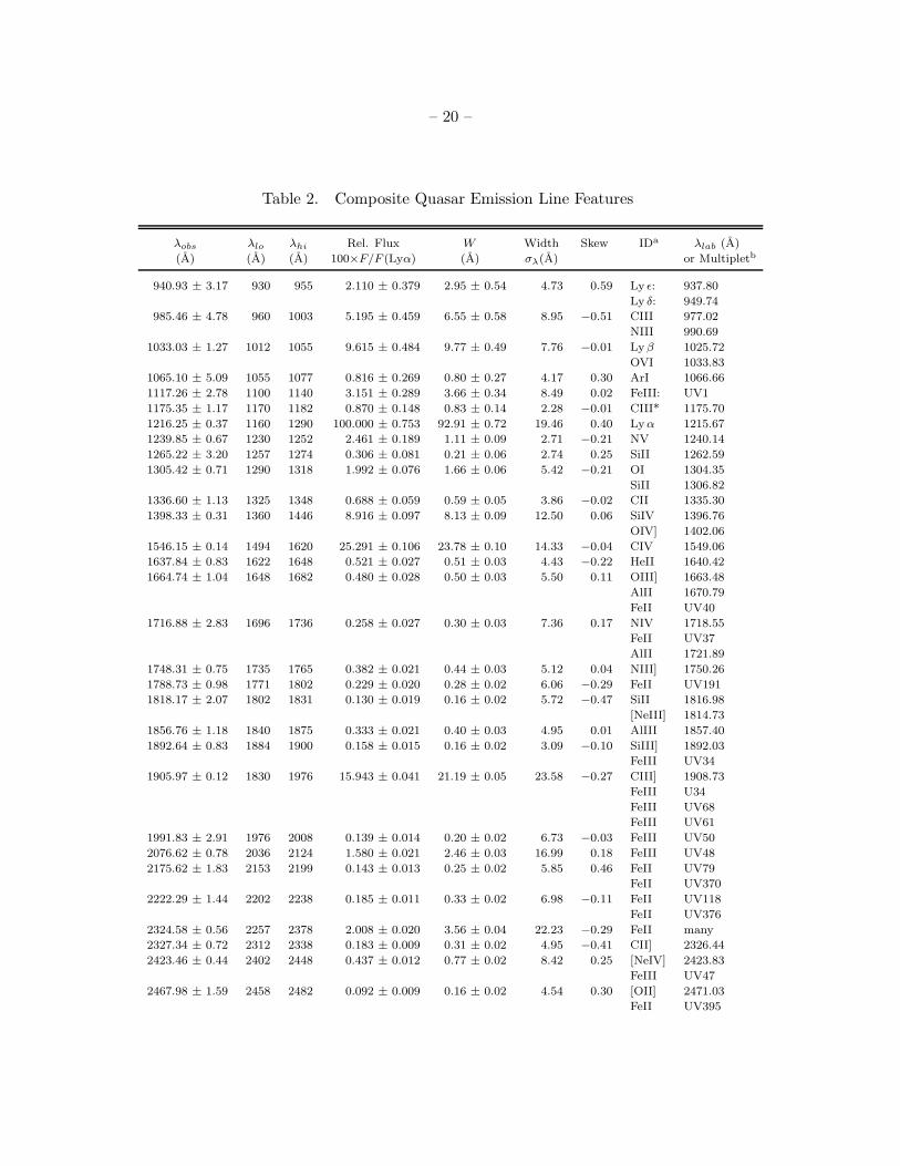
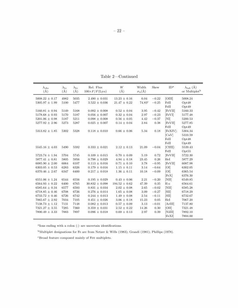
taken from those references. Table 2 lists the detected lines, their vacuum wavelength peak positions,

relative fluxes, equivalent widths, profile widths, skewness, and identifications. Rest wavelengths

were taken from the Atomic Line List28. Wavelengths of lines consisting of multiple transitions

were found by taking the oscillator-strength weighted average in the case of permitted lines, and

the adopted values from the above references for forbidden lines. In all cases, the permitted rest

wavelength values agreed with the (vacuum) values adopted in the above references. Fig. 6 shows

an expanded view of the quasar composite on a log-linear scale with the emission features labeled.

It is clear from Fig. 6 that most of the UV-optical continuum is populated by emission lines.

Most strong emission lines show “contamination” by blends with weaker lines, as seen in the

expanded profiles of 12 emission line regions in Fig. 7. The very broad conspicuous feature from

28The Atomic Line List is hosted by the Department of Physics and Astronomy at the University of Kentucky;

(http://www.pa.uky.edu/∼peter/atomic/).

– 12 –

≈ 2200 − 4000 A is known as the 3000 A bump (Grandi 1982; Oke, Shields & Korycansky 1984),

and consists of blends of Fe ii line emission and Balmer continuum emission (Wills, Netzer & Wills

1985). The Fe ii and Fe iii complexes are particularly ubiquitous, and contribute a large fraction of

the emission line flux. Using this composite, these complexes have been shown to be an important

contributor to the color-redshift relationships of quasars (Richards et al. 2001a).

Several absorption features often seen in galaxies are also identifiable in the median composite

quasar spectrum. These lines are listed in Table 3 along with several measured quantities, and

include H9 λ3835, H 10 λ3797, the Ca ii λ3933 K line, and Ca ii λλ8498, 8542 – two lines of a

triplet (the second-weakest third component would fall beyond the red end of the spectrum). The

MgI λλ5167, 5172, 5183 triplet lines may also be present in the spectrum, but they would lie inside

a strong complex of Feii emission and near several other expected emission lines. The locations of

other common stellar absorption lines seen in galaxies, such as the lower-order Balmer lines and the

Ca ii λ3968 H line, are dominated by emission lines. The presence of stellar absorption lines argues

for at least some host galaxy contamination in the quasar composite spectrum, despite the fact that

we rejected objects with obvious stellar lines in individual galaxies. To examine this further, we

have created a low-redshift median composite using only quasars with redshifts zem ≤ 0.5, which

is almost equivalent to selecting only quasars with restframe absolute r′ magnitude Mr′ ≥ −21.5

(calculated using a spectral index of αν = −0.44). The low-z composite covers a rest wavelength

range of 2550− 8555A. The absorption lines found in the low-z spectrum are marked in Fig. 8, and

listed in Table 3. More absorption lines are detected in the low-z composite spectrum than the

full-dataset spectrum, and the lines in common are stronger in the low-z spectrum – as expected if

host galaxy contamination is the source of the absorption lines. We discuss the absorption lines in

more detail in § 5.

The 2175A extinction bump often seen in the spectra of objects observed through the Galactic

diffuse interstellar medium, and usually attributed to graphite grains (Mathis, Rumpl & Nordsieck

1977), is not present at a detectable level in the composite spectrum. This agrees with the non-

detection of the feature by Pitman, Clayton & Gordon (2000) who searched for it in other quasar

spectral composites.

4.3. Systematic Line Shifts

Because the composite was constructed using redshifts based upon a single emission line posi-

tion ([O iii] λ5007) or cross-correlations with an [O iii]-based composite, we can check for systematic

offsets between the measured peak positions and the [O iii]-based wavelengths. Several emission

lines – C iv λ1549 for example – are offset from their laboratory wavelengths, as evident from Fig. 7.

Such line shifts have been detected previously (e.g. Grandi 1982; Wilkes 1986; Tytler & Fan 1992;

Laor et al. 1995; McIntosh, Rix, Rieke & Foltz 1999), and are present for many of the lines listed

in Table 2. Real line position offsets can be confused with apparent “shifts” which can arise from

several sources, including contamination by line blends, incorrect identifications, and line asymme-

– 13 –

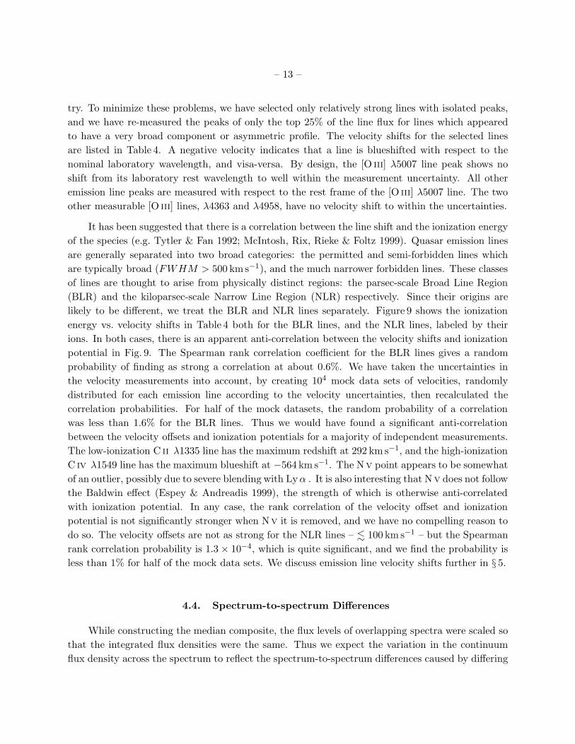
try. To minimize these problems, we have selected only relatively strong lines with isolated peaks,

and we have re-measured the peaks of only the top 25% of the line flux for lines which appeared

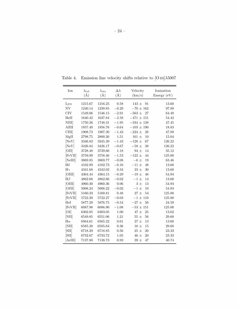
to have a very broad component or asymmetric profile. The velocity shifts for the selected lines

are listed in Table 4. A negative velocity indicates that a line is blueshifted with respect to the

nominal laboratory wavelength, and visa-versa. By design, the [O iii] λ5007 line peak shows no

shift from its laboratory rest wavelength to well within the measurement uncertainty. All other

emission line peaks are measured with respect to the rest frame of the [O iii] λ5007 line. The two

other measurable [O iii] lines, λ4363 and λ4958, have no velocity shift to within the uncertainties.

It has been suggested that there is a correlation between the line shift and the ionization energy

of the species (e.g. Tytler & Fan 1992; McIntosh, Rix, Rieke & Foltz 1999). Quasar emission lines

are generally separated into two broad categories: the permitted and semi-forbidden lines which

are typically broad (FWHM > 500 kms−1), and the much narrower forbidden lines. These classes

of lines are thought to arise from physically distinct regions: the parsec-scale Broad Line Region

(BLR) and the kiloparsec-scale Narrow Line Region (NLR) respectively. Since their origins are

likely to be different, we treat the BLR and NLR lines separately. Figure 9 shows the ionization

energy vs. velocity shifts in Table 4 both for the BLR lines, and the NLR lines, labeled by their

ions. In both cases, there is an apparent anti-correlation between the velocity shifts and ionization

potential in Fig. 9. The Spearman rank correlation coefficient for the BLR lines gives a random

probability of finding as strong a correlation at about 0.6%. We have taken the uncertainties in

the velocity measurements into account, by creating 104 mock data sets of velocities, randomly

distributed for each emission line according to the velocity uncertainties, then recalculated the

correlation probabilities. For half of the mock datasets, the random probability of a correlation

was less than 1.6% for the BLR lines. Thus we would have found a significant anti-correlation

between the velocity offsets and ionization potentials for a majority of independent measurements.

The low-ionization C ii λ1335 line has the maximum redshift at 292 km s−1, and the high-ionization

C iv λ1549 line has the maximum blueshift at −564 km s−1. The Nv point appears to be somewhat

of an outlier, possibly due to severe blending with Lyα . It is also interesting that Nv does not follow

the Baldwin effect (Espey & Andreadis 1999), the strength of which is otherwise anti-correlated

with ionization potential. In any case, the rank correlation of the velocity offset and ionization

potential is not significantly stronger when Nv it is removed, and we have no compelling reason to

do so. The velocity offsets are not as strong for the NLR lines – . 100 km s−1 – but the Spearman

rank correlation probability is 1.3× 10−4, which is quite significant, and we find the probability is

less than 1% for half of the mock data sets. We discuss emission line velocity shifts further in § 5.

4.4. Spectrum-to-spectrum Differences

While constructing the median composite, the flux levels of overlapping spectra were scaled so

that the integrated flux densities were the same. Thus we expect the variation in the continuum

flux density across the spectrum to reflect the spectrum-to-spectrum differences caused by differing

– 14 –

continuum shapes and emission line fluxes and profiles. (This does not, however, address spectral

time variability.) Fig. 10 shows the 68% semi-interquantile range divided by the median spectrum,

after the contribution from the combined flux density uncertainties of each spectrum were removed

in quadrature. The individual spectral uncertainties include statistical noise estimates, but not

uncertainties in the (un-finalized) flux calibration. The largest relative variations from the median

spectrum occur in the narrow emission lines such as the [O iii] λλ4958, 5007 lines, and the cores of

broad emission lines such as C iv λ1549 and Lyα λ1215. Variations of the broad components of Hα

λ6563 and Mg ii λ2798 are evident, but less so for Hβ λ4861 and C iv λ1549, and there is little sign

of variation in the C iii] λ1908 line. Most of the broad Fe ii complexes show significant variation.

The Lyα forest region varies considerably, as expected, since structure in the forest can be partly

resolved in the individual spectra, and the forest strength changes with redshift so the combination

of spectra at different redshifts will naturally give rise to a high variance. An additional feature of

some interest is the pair of variation peaks at 3935 A and 3970 A, which correspond precisely to the

Ca ii doublet. These are detected in absorption in the median composites (although [Ne iii] and

H ǫ emission interfere with Ca iiλ3970), and the variation may indicate that spectral contamination

by the host galaxy is fairly common. A full analysis of spectrum-to-spectrum variations requires

other means such as principal component analysis (Boroson & Green 1992; Francis, Hewett, Foltz

& Chaffee 1992; Brotherton, Wills, Francis & Steidel 1994; Wills et al. 1999), which we plan for a

future project.

5. Discussion

The Large Bright quasar Survey (LBQS) composite (kindly provided by S. Morris) updated

from Francis et al. (1991), the First Bright quasar Survey (FBQS) composite (available electron-

ically, Brotherton et al. (2000)), and our median composite, are shown for comparison in Fig. 11.

The spectra have been scaled to unit average flux density in the range 3020 − 3100A. All three

spectra are quite similar in appearance except for slight differences. The strength of the Lyα line

and some of the narrow emission lines in the FBQS composite are stronger than for the other

composites. The difference is probably due to that fact that the FBQS sample is entirely radio

selected, and there is a correlation between line strengths and radio loudness (Boroson & Green

1992; Francis, Hewett, Foltz & Chaffee 1992; Brotherton, Wills, Francis & Steidel 1994; Wills et

al. 1999). Otherwise, the relative fluxes are similar for the lines in common among the various

composites. The higher resolution and higher S/N of our composite has allowed us to identify

many more lines than listed for the other spectra (although a number of the features we find are

present at a lower significance level in the other spectra). We have identified a total of 85 emission

features in the median spectrum. All of the features have been identified in other quasar or AGN

spectra, but not in any single object. A large number of the identified features are attributed to

either Fe ii or Fe iii multiplets. The combination of these features has been shown to greatly affect

the color-redshift relationship for quasars (Richards et al. 2001a).

– 15 –

A single power-law is an adequate fit to the continuum between Lyα and Hβ , especially given

the predicted strengths of the Fe ii and Fe iii emission line complexes in that range (Verner et al.

1999; Netzer & Wills 1983; Laor, Jannuzi, Green & Boroson 1997). The index we find, αν = −0.44,

is in good agreement with most recent values found in optically-selected quasar samples. Table 5

lists average power-law indices from various sources over the past decade. The LBQS composite,

FBQS composite, and Hubble Space Telescope (HST) composite (Zheng et al. 1997) spectra are

available electronically, so for consistency, we have also remeasured the power-law indices of those

spectra using the technique described in § 4.1. The remeasured values are not significantly different

from the values given in the papers.

Most of the composite measurements agree with averages over continuum fits to individual

spectra. One outlier is the measurement by Zheng et al. (1997), who find a steeper (redder)

continuum with αν = −0.99 using a composite made with spectra from HST. The difference is

attributed to the lower redshift of the Zheng et al. (1997) quasar sample and a correlation between

redshift and steeper UV continuum (Francis 1993). To test this, we have created a low-redshift

geometric mean composite using only those quasars which cover a rest wavelength of 5000 A (z <

0.84). Since the 1350A wavelength region we have used to measure continuum slopes is not covered

by the low-z composite, we used instead the flux density in the wavelength range 3020 − 3100A

multiplied by a factor of 0.86, which is the ratio of the flux density of the power-law fit to the

flux density of the spectrum for the full-sample geometric mean composite in that range. We find

a steeper index for the low-redshift composite, αν = −0.65, than for the full-sample composite,

αν = −0.44, although the difference is not as great as with the Zheng et al. (1997) composite.

Another apparently discrepant value is the result from Schneider et al. (2001), who find αν =

−0.93 for a sample of very high-redshift quasars. Similar values for high-z samples have been found

by Fan et al. (2001) and Schneider, Schmidt & Gunn (1991). The steep indices measured for high-z

quasars may be due to the restricted wavelength range typically used in fitting the continua, as

suggested by Schneider et al. (2001), and not to a change in the underlying spectral index at high

redshift. At high redshifts, only relatively short wavelength ranges redward of Lyα are avaliable

in optical spectra, and these tend to be populated by broad Fe ii and Fe iii complexes. If, for

example, the regions of the median composite near 1350A and 1600A (just redward of the C iv

emission line) are taken as continuum (as Schneider et al. (2001) did), we find a power-law index

of αν = −0.93. This example demonstrates the generic difficulty of measuring continuum indices

without a very large range of wavelength, or some estimate of the strength of the contribution from

blended emission lines.

The continuum slope changes abruptly near 5000 A and becomes steeper with an index of

αν = −2.45, which is a good fit up to the red end of the spectrum (8555 A). This change is also

evident in the FBQS composite, and has been noted in the spectra of individual quasars (Wills,

Netzer & Wills 1985). An upturn in the spectral energy distribution of quasars – the so-called

near-infrared inflection, presumably caused by emission from hot dust – has been seen starting

between 0.7 and 1.5µm (e.g. Neugebauer et al. 1987; Elvis et al. 1994). This may be in part what

– 16 –

we are seeing at wavelengths beyond ≈ 5000A, but it is unlikely that the sublimation temperature

of dust would be high enough for the emission to extend to wavelengths below 6000A (Puget, Leger,

& Boulanger 1985; Efstathiou, Hough, & Young 1995).

Another possible contributor to the long wavelength steepening is contamination from the

host galaxies. The 3′′ optical fiber diameter subtends much if not all of the host galaxy image,

even for the lowest redshift quasars. The best evidence for the contribution of host galaxy light

is the presence of stellar absorption lines in the composite spectra. The lines become stronger as

the redshift, and equivalently, luminosity, distributions of the quasar sample are lowered. This

is seen by comparing the absorption line strengths of the low-redshift median composite (§ 4.2)

with the full-sample composite. The strengths of the absorption lines in the low-redshift median

composite, assuming a typical elliptical galaxy spectrum, imply a contribution to the composite

quasar light from stars of about 7− 15% at the locations of Ca ii λ3933 and Na iλ5896, and about

30% at the locations of Ca iiλλ8498, 8542. The trend of a greater contribution from starlight with

increasing wavelength is expected because the least luminous quasars, in which the relative host

galaxy light is presumably most important, contribute the majority of spectra to the composite

at longer wavelengths. This trend has also been seen in the spectral light from the nuclei of

individual low-redshift Seyfert galaxies and other AGN (Terlevich, Diaz, & Terlevich 1990; Serote

Roos, Boisson, Joly, & Ward 1998), which suggest a significant contribution from starburst activity

dominated by red supergiants (Cid Fernandes & Terlevich 1995). The mean absolute r′ magnitude

of the quasars making up the low-z composite is Mr′ = −21.7 (Fig. 1), which implies a host galaxy

magnitude of about Mr′ = −19.2 (assuming a host contribution of ∼ 10%) – a moderately luminous

value in the SDSS filter system (Blanton et al. 2001). We conclude that both stellar light from the

host galaxies and a real change in the quasar continuum cause the steepening of the spectral index

beyond 5000A.

The detection of stellar Balmer absorption lines implies that young or intermediate age stars

make a substantial contribution to the light of the host galaxies. This is at odds with the conclusions

based on host-galaxy spectra (Nolan et al. 2001), and two-dimensional image modeling (McLure

et al. 1999; McLure & Dunlop 2000) that the hosts of quasars and radio galaxies are “normal”

giant ellipticals. The discrepancy cannot immediately be attributed to redshift differences, since

the McLure & Dunlop (2000) sample extends to z ≈ 1, and we detect Balmer absorption lines in

the full-sample composite with a mean redshift of z = 1.25. More likely, the difference is due to the

fact that our spectra include only the inner 3′′ of the galaxy light while the spectra taken by Nolan

et al. (2001) sample only off-nuclear (5′′ from nucleus) light, and the image modeling includes the

entire profile of the galaxies. This suggests that the stellar population near the nuclei of quasar host

galaxies – near the quasars themselves – is substantially younger than that of the host galaxies.

Velocity shifts in the BLR lines relative to the forbidden NLR lines – taken to be at the

systemic host-galaxy redshift – are seen for most quasars and are similar to the values we find

for the composite BLR lines relative to [O iii] λ5007 (e.g. Tytler & Fan 1992; Laor et al. 1995;

McIntosh, Rix, Rieke & Foltz 1999). The origin of the shifts is not known, but explanations

– 17 –

include gas inflows and outflows (e.g. Gaskell 1982; Corbin 1990), attenuation by dust (Grandi

1977; Heckman, Butcher, Miley & van Breugel 1981), relativistic effects (Netzer 1977; Corbin 1995,

1997; McIntosh, Rix, Rieke & Foltz 1999), and line emission from physically different locations

(e.g. Espey et al. 1989). The magnitudes of the shifts seem to depend upon the ionization energies

(Gaskell 1982; Wilkes 1986; Espey et al. 1989; Tytler & Fan 1992; McIntosh, Rix, Rieke & Foltz

1999) in the sense that more negative velocities (blueshifts) are seen for higher ionization lines. We

have confirmed this correlation using a large number of BLR lines (§ 4.3).

It is often assumed that the NLR lines are at the systemic redshift of the quasar, since the

lines are thought to originate in a kpc-scale region centered on the quasar, and the lines show

good agreement (to within 100 km s−1) with the redshifts of host galaxies determined by stellar

absorption lines (Gaskell 1982; Vrtilek & Carleton 1985), and H i 21 cm observations (Hutchings,

Gower & Price 1987). However, for some of the higher-ionization forbidden lines, such as [O iii]

λ5007, Nevλ3426, Feviiλ6086, Fexλ6374, and Fexiλ7892, seen in quasars and Seyfert galaxies,

significant velocity shifts, usually blueshifts, have been detected in the past (Heckman, Butcher,

Miley & van Breugel 1981; Mirabel & Wilson 1984; Penston et al. 1984; Whittle 1985; Appenzeller

& Wagner 1991, e.g.). The large number (17) of NLR lines we have been able to measure cover

a wide range in ionization potentials. These lines are shifted with respect to one another and the

shifts are correlated with ionization energy. This appears to be a real effect, since we have been

careful to select only those lines which have well-defined non-blended peaks. Another verification

of the accuracy of the velocity measurements is that lines originating from the same ion but at

different rest wavelengths almost always have consistent velocity offsets within the measurement

uncertainties (Table 4 & Fig. 9).

The NLR velocity shifts and their correlation with ionization potential suggest that the same

mechanism responsible for the shifts of the BLR lines also applies to the NLR lines, although the

effect is weaker. One possible explanation is that the BLR contains some lower density forbidden

line emitting gas, as first suggested by Penston (1977). The correlation is strong, but the effect

is subtle, so follow-up work will likely have to involve both higher quality optical spectra and

observations in the near-IR in order to detect a sufficient sample of narrow forbidden lines.

We have implicitly assumed that the velocity differences are independent of other factors such

as redshift and luminosity. However, McIntosh, Rix, Rieke & Foltz (1999) found that higher-z

quasars tend to have greater velocity offsets relative to the [O iii] line. For quasars in our sample

with z > 0.84, the [O iii] emission line is redshifted out of the spectra, which is why we used

a cross-correlation technique to estimate the center-of-mass redshifts. If the true velocity offsets

depend upon redshift, the relation will be weakened by the cross-correlation matching which finds

the best match to a lower-redshift template, and thus will tend to yield the lower-redshift emission

line positions. A desirable future project is extending the wavelength coverage to the near-infrared

at higher redshift and to the ultraviolet at lower redshift in order to simultaneously detect low

and high velocity lines. Such a program of even a relatively modest sample size would be highly

beneficial to many quasar studies.

– 18 –

6. Summary

We have created median and geometric mean composite quasar spectra using a sample of over

2200 quasars in the Sloan Digital Sky Survey. The resolution and signal to noise ratio exceed

all previously published UV/optical quasar composites. Over 80 emission line features have been

detected and identified. We have been able to measure velocity shifts in a large number of both

permitted and forbidden emission line peaks, most of which have no such previous measurements.

Power-law fits to the continua verify the results from most recent studies. The composites show

that there is a lack of emission-free regions across most of the UV/optical wavelength range, which

makes fitting quasar continua difficult unless a very wide wavelength range is available.

The SDSS is rapidly producing high-quality spectra of quasars which cover a wide range of

properties. Composite spectra can therefore be made from numerous sub-samples in order to

search for dependencies of global spectral characteristics on a variety of quasar parameters, such

as redshift, luminosity, and radio loudness – a program which is currently underway. We are also

using other techniques such as principal component analysis to examine trends among the diversity

of quasar spectra.

The median composite is being used as a cross-correlation template for spectra in the SDSS,

and many other applications are imaginable. The median composite spectrum is likely to be of

general interest, so it is available as an electronic table (Table 1).

The Sloan Digital Sky Survey (SDSS)29 is a joint project of The University of Chicago, Fermi-

lab, the Institute for Advanced Study, the Japan Participation Group, The Johns Hopkins Univer-

sity, the Max-Planck-Institute for Astronomy, New Mexico State University, Princeton University,

the United States Naval Observatory, and the University of Washington. Apache Point Observa-

tory, site of the SDSS telescopes, is operated by the Astrophysical Research Consortium (ARC).

Funding for the project has been provided by the Alfred P. Sloan Foundation, the SDSS member

institutions, the National Aeronautics and Space Administration, the National Science Foundation,

the U.S. Department of Energy, Monbusho, and the Max Planck Society. We thank Simon Morris

for making an electronic version of the LBQS composite quasar spectrum available to us, and Bev

Wills for helpful comments. MAS acknowledges support of NSF grant AST-0071091. DPS and

GTR acknowledges support of NSF grant AST-990703.

29The SDSS Web site is http://www.sdss.org/.

– 19 –

Table 1. Median Composite Quasar Spectruma

λ fλ fλ Uncertainty

(A) (Arbitrary Units) (Arbitrary Units)

800.5 0.149 0.074

801.5 0.000 0.260

802.5 0.676 0.227

803.5 0.000 0.222

804.5 0.413 0.159

805.5 0.338 0.326

806.5 0.224 0.159

807.5 0.122 0.360

808.5 0.612 0.346

809.5 0.752 0.304

810.5 0.197 0.257

811.5 0.187 0.189

812.5 0.000 0.126

813.5 0.000 0.171

814.5 0.502 0.181

Note. — The complete version of this table

will appear in the electronic edition of the Jour-

nal. The printed edition contains only a sample.

The full table can be found temporarily at

ftp://sdss.fnal.gov/pub/danvb/qsocomposite/sdss qso median.tab1

– 20 –

Table 2. Composite Quasar Emission Line Features

λobs λlo λhi Rel. Flux W Width Skew IDa λlab (A)

(A) (A) (A) 100×F/F (Lyα) (A) σλ(A) or Multipletb

940.93 ± 3.17 930 955 2.110 ± 0.379 2.95 ± 0.54 4.73 0.59 Ly ǫ: 937.80

Ly δ: 949.74

985.46 ± 4.78 960 1003 5.195 ± 0.459 6.55 ± 0.58 8.95 −0.51 CIII 977.02

NIII 990.69

1033.03 ± 1.27 1012 1055 9.615 ± 0.484 9.77 ± 0.49 7.76 −0.01 Lyβ 1025.72

OVI 1033.83

1065.10 ± 5.09 1055 1077 0.816 ± 0.269 0.80 ± 0.27 4.17 0.30 ArI 1066.66

1117.26 ± 2.78 1100 1140 3.151 ± 0.289 3.66 ± 0.34 8.49 0.02 FeIII: UV1

1175.35 ± 1.17 1170 1182 0.870 ± 0.148 0.83 ± 0.14 2.28 −0.01 CIII* 1175.70

1216.25 ± 0.37 1160 1290 100.000 ± 0.753 92.91 ± 0.72 19.46 0.40 Lyα 1215.67

1239.85 ± 0.67 1230 1252 2.461 ± 0.189 1.11 ± 0.09 2.71 −0.21 NV 1240.14

1265.22 ± 3.20 1257 1274 0.306 ± 0.081 0.21 ± 0.06 2.74 0.25 SiII 1262.59

1305.42 ± 0.71 1290 1318 1.992 ± 0.076 1.66 ± 0.06 5.42 −0.21 OI 1304.35

SiII 1306.82

1336.60 ± 1.13 1325 1348 0.688 ± 0.059 0.59 ± 0.05 3.86 −0.02 CII 1335.30

1398.33 ± 0.31 1360 1446 8.916 ± 0.097 8.13 ± 0.09 12.50 0.06 SiIV 1396.76

OIV] 1402.06

1546.15 ± 0.14 1494 1620 25.291 ± 0.106 23.78 ± 0.10 14.33 −0.04 CIV 1549.06

1637.84 ± 0.83 1622 1648 0.521 ± 0.027 0.51 ± 0.03 4.43 −0.22 HeII 1640.42

1664.74 ± 1.04 1648 1682 0.480 ± 0.028 0.50 ± 0.03 5.50 0.11 OIII] 1663.48

AlII 1670.79

FeII UV40

1716.88 ± 2.83 1696 1736 0.258 ± 0.027 0.30 ± 0.03 7.36 0.17 NIV 1718.55

FeII UV37

AlII 1721.89

1748.31 ± 0.75 1735 1765 0.382 ± 0.021 0.44 ± 0.03 5.12 0.04 NIII] 1750.26

1788.73 ± 0.98 1771 1802 0.229 ± 0.020 0.28 ± 0.02 6.06 −0.29 FeII UV191

1818.17 ± 2.07 1802 1831 0.130 ± 0.019 0.16 ± 0.02 5.72 −0.47 SiII 1816.98

[NeIII] 1814.73

1856.76 ± 1.18 1840 1875 0.333 ± 0.021 0.40 ± 0.03 4.95 0.01 AlIII 1857.40

1892.64 ± 0.83 1884 1900 0.158 ± 0.015 0.16 ± 0.02 3.09 −0.10 SiIII] 1892.03

FeIII UV34

1905.97 ± 0.12 1830 1976 15.943 ± 0.041 21.19 ± 0.05 23.58 −0.27 CIII] 1908.73

FeIII U34

FeIII UV68

FeIII UV61

1991.83 ± 2.91 1976 2008 0.139 ± 0.014 0.20 ± 0.02 6.73 −0.03 FeIII UV50

2076.62 ± 0.78 2036 2124 1.580 ± 0.021 2.46 ± 0.03 16.99 0.18 FeIII UV48

2175.62 ± 1.83 2153 2199 0.143 ± 0.013 0.25 ± 0.02 5.85 0.46 FeII UV79

FeII UV370

2222.29 ± 1.44 2202 2238 0.185 ± 0.011 0.33 ± 0.02 6.98 −0.11 FeII UV118

FeII UV376

2324.58 ± 0.56 2257 2378 2.008 ± 0.020 3.56 ± 0.04 22.23 −0.29 FeII many

2327.34 ± 0.72 2312 2338 0.183 ± 0.009 0.31 ± 0.02 4.95 −0.41 CII] 2326.44

2423.46 ± 0.44 2402 2448 0.437 ± 0.012 0.77 ± 0.02 8.42 0.25 [NeIV] 2423.83

FeIII UV47

2467.98 ± 1.59 2458 2482 0.092 ± 0.009 0.16 ± 0.02 4.54 0.30 [OII] 2471.03

FeII UV395

– 21 –

Table 2—Continued

λobs λlo λhi Rel. Flux W Width Skew IDa λlab (A)

(A) (A) (A) 100×F/F (Lyα) (A) σλ(A) or Multipletb

2626.92 ± 0.99 2595 2654 0.398 ± 0.013 0.81 ± 0.03 9.93 0.00 FeII UV1

2671.89 ± 1.78 2657 2684 0.067 ± 0.008 0.14 ± 0.02 5.10 0.05 AlII] 2669.95

OIII 2672.04

2800.26 ± 0.10 2686 2913 14.725 ± 0.030 32.28 ± 0.07 34.95 −0.06 MgII 2798.75

2964.28 ± 0.79 2910 3021 2.017 ± 0.017 4.93 ± 0.04 22.92 −0.03 FeII UV78

3127.70 ± 1.07 3100 3153 0.326 ± 0.012 0.86 ± 0.03 9.38 −0.13 OIII 3133.70

FeII Opt82

3191.78 ± 0.99 3159 3224 0.445 ± 0.013 1.17 ± 0.03 12.77 −0.04 HeI 3188.67

FeII Opt6

FeII Opt7

3261.40 ± 2.70 3248 3272 0.032 ± 0.008 0.09 ± 0.02 3.27 0.06 FeI Opt91

FeII Opt1

3281.74 ± 3.15 3272 3297 0.036 ± 0.008 0.10 ± 0.02 4.39 0.56 FeII Opt1

3345.39 ± 0.75 3329 3356 0.118 ± 0.008 0.35 ± 0.02 5.50 −0.41 [NeV] 3346.82

3425.66 ± 0.46 3394 3446 0.405 ± 0.012 1.22 ± 0.04 9.09 −0.62 [NeV] 3426.84

3498.92 ± 1.60 3451 3537 0.432 ± 0.014 1.38 ± 0.05 16.79 −0.24 FeII Opt4

FeII Opt16

3581.70 ± 4.48 3554 3613 0.100 ± 0.011 0.34 ± 0.04 7.98 0.79 [FeVII] 3587.34

HeI 3588.30

3729.66 ± 0.18 3714 3740 0.424 ± 0.009 1.56 ± 0.03 3.32 −0.24 [OII] 3728.48

3758.46 ± 0.56 3748 3771 0.078 ± 0.007 0.29 ± 0.03 3.71 0.12 [FeVII] 3759.99

3785.47 ± 1.31 3775 3799 0.056 ± 0.006 0.22 ± 0.03 4.24 0.13 FeII: Opt15

3817.41 ± 2.46 3800 3832 0.124 ± 0.007 0.51 ± 0.03 7.33 −0.10 FeII: Opt14

3869.77 ± 0.25 3850 3884 0.345 ± 0.008 1.38 ± 0.03 5.31 −0.50 [NeIII] 3869.85

3891.03 ± 1.28 3882 3898 0.020 ± 0.005 0.08 ± 0.02 2.02 −0.27 HeI 3889.74

H8 3890.15

3968.43 ± 0.91 3950 3978 0.104 ± 0.007 0.45 ± 0.03 5.32 −0.62 [NeIII] 3968.58

H ǫ 3971.20

4070.71 ± 1.18 4061 4079 0.039 ± 0.005 0.18 ± 0.03 3.20 0.01 [FeV] 4072.39

[SII] 4073.63

4102.73 ± 0.66 4050 4152 1.066 ± 0.013 5.05 ± 0.06 18.62 0.03 H δ 4102.89

4140.50 ± 0.96 4135 4145 0.026 ± 0.004 0.13 ± 0.02 1.83 −0.38 FeII Opt27

FeII Opt28

4187.55 ± 1.97 4157 4202 0.154 ± 0.009 0.76 ± 0.04 9.77 −0.40 FeII Opt27

FeII Opt28

4239.85 ± 2.07 4227 4260 0.107 ± 0.008 0.53 ± 0.04 5.73 −0.05 [FeII] Opt21F

4318.30 ± 0.78 4315 4328 0.038 ± 0.005 0.17 ± 0.02 2.31 0.58 [FeII] Opt21F

FeII Opt32

4346.42 ± 0.38 4285 4412 2.616 ± 0.017 12.62 ± 0.08 20.32 0.12 H γ 4341.68

4363.85 ± 0.68 4352 4372 0.110 ± 0.007 0.46 ± 0.03 3.10 −0.18 [OIII] 4364.44

4478.22 ± 1.13 4469 4484 0.029 ± 0.006 0.14 ± 0.03 2.20 −0.69 FeII Opt37

HeI: 4472.76

4564.71 ± 1.56 4435 4762 3.757 ± 0.029 19.52 ± 0.15 61.69c 0.23 FeII Opt37

FeII Opt38

4686.66 ± 1.04 4668 4696 0.139 ± 0.009 0.72 ± 0.05 5.92 −0.57 HeII 4687.02

4853.13 ± 0.41 4760 4980 8.649 ± 0.030 46.21 ± 0.16 40.44 0.61 Hβ 4862.68

4930.75 ± 1.13 4920 4941 0.082 ± 0.007 0.40 ± 0.04 3.98 −0.02 FeII Opt42

4960.36 ± 0.22 4945 4972 0.686 ± 0.014 3.50 ± 0.07 3.85 −0.22 [OIII] 4960.30

– 22 –

Table 2—Continued

λobs λlo λhi Rel. Flux W Width Skew IDa λlab (A)

(A) (A) (A) 100×F/F (Lyα) (A) σλ(A) or Multipletb

5008.22 ± 0.17 4982 5035 2.490 ± 0.031 13.23 ± 0.16 6.04 −0.22 [OIII] 5008.24

5305.97 ± 1.99 5100 5477 3.522 ± 0.036 21.47 ± 0.22 74.83c −0.25 FeII Opt48

FeII Opt49

5160.81 ± 0.94 5149 5168 0.092 ± 0.008 0.52 ± 0.04 3.95 −0.42 [FeVII] 5160.33

5178.68 ± 0.93 5170 5187 0.056 ± 0.007 0.32 ± 0.04 2.97 −0.23 [FeVI] 5177.48

5201.06 ± 0.98 5187 5211 0.098 ± 0.008 0.56 ± 0.05 4.42 −0.37 [NI] 5200.53

5277.92 ± 2.96 5273 5287 0.025 ± 0.007 0.14 ± 0.04 2.84 0.38 [FeVII] 5277.85

FeII Opt49

5313.82 ± 1.85 5302 5328 0.118 ± 0.010 0.66 ± 0.06 5.34 0.18 [FeXIV]: 5304.34

[CaV] 5310.59

FeII Opt48

FeII Opt49

5545.16 ± 4.03 5490 5592 0.333 ± 0.021 2.12 ± 0.13 21.09 −0.04 [ClIII]: 5539.43

FeII Opt55

5723.74 ± 1.94 5704 5745 0.109 ± 0.015 0.70 ± 0.09 5.19 0.72 [FeVII] 5722.30

5877.41 ± 0.81 5805 5956 0.798 ± 0.029 4.94 ± 0.18 23.45 0.26 HeI 5877.29

6085.90 ± 2.00 6064 6107 0.113 ± 0.016 0.71 ± 0.10 3.78 −0.95 [FeVII] 6087.98

6303.05 ± 0.53 6283 6326 0.179 ± 0.016 1.15 ± 0.11 3.14 −0.64 [OI] 6302.05

6370.46 ± 2.67 6347 6400 0.217 ± 0.018 1.36 ± 0.11 10.18 −0.09 [OI] 6365.54

[FeX] 6376.30

6551.06 ± 1.24 6544 6556 0.195 ± 0.029 0.43 ± 0.06 2.21 −0.20 [NII] 6549.85

6564.93 ± 0.22 6400 6765 30.832 ± 0.098 194.52 ± 0.62 47.39 0.35 Hα 6564.61

6585.64 ± 0.34 6577 6593 0.831 ± 0.034 2.02 ± 0.08 2.65 −0.02 [NII] 6585.28

6718.85 ± 0.46 6708 6726 0.276 ± 0.014 1.65 ± 0.08 3.09 −0.27 [SII] 6718.29

6733.72 ± 0.46 6726 6742 0.244 ± 0.013 1.49 ± 0.08 2.54 −0.11 [SII] 6732.67

7065.67 ± 2.92 7034 7105 0.451 ± 0.026 3.06 ± 0.18 15.23 0.05 HeI 7067.20

7138.73 ± 1.12 7131 7148 0.082 ± 0.013 0.57 ± 0.09 3.13 −0.01 [ArIII] 7137.80

7321.27 ± 3.55 7285 7360 0.359 ± 0.031 2.52 ± 0.22 14.26 0.30 [OII] 7321.48

7890.49 ± 3.33 7883 7897 0.096 ± 0.018 0.69 ± 0.13 2.97 0.39 [NiIII] 7892.10

[FeXI] 7894.00

aIons ending with a colon (:) are uncertain identifications.

bMultiplet designations for Fe are from Netzer & Wills (1983); Grandi (1981); Phillips (1978).

cBroad feature composed mainly of Feii multiplets.

– 23 –

Table 3. Composite Quasar Absorption Line Features

λobs W Width ID λlab

(A) (A) σλ(A) (A)

Median Composite Using All Spectra

3800.38 ± 1.09 0.35 ± 0.03 4.14 H10 3798.98

3837.12 ± 1.49 0.46 ± 0.03 5.96 H9 3836.47

3934.96 ± 0.55 0.91 ± 0.03 7.11 Ca ii 3934.78

8502.80 ± 7.22 1.11 ± 0.61 3.85 Ca ii 8500.36

8544.17 ± 1.89 2.22 ± 0.44 3.87 Ca ii 8544.44

Low-Redshift Median Composite (zem ≤ 0.5)

3737.82 ± 1.03 0.16 ± 0.03 0.97 H13: 3735.43

3749.45 ± 1.13 0.31 ± 0.04 2.96 H12: 3751.22

3774.09 ± 1.27 0.36 ± 0.04 3.56 H11 3771.70

3799.71 ± 0.89 0.84 ± 0.05 4.86 H10 3798.98

3837.77 ± 1.16 0.95 ± 0.05 5.69 H9 3836.47

3934.94 ± 0.48 1.64 ± 0.06 6.94 Ca ii 3934.78

3974.66 ± 0.88 0.36 ± 0.04 2.42 Ca iia 3969.59

5892.66 ± 1.24 0.44 ± 0.05 3.72 Na ii 5891.58

5897.56

8502.80 ± 7.22 1.11 ± 0.61 3.85 Ca ii 8500.36

8544.17 ± 1.89 2.22 ± 0.44 3.87 Ca ii 8544.44

aContaminated by emssion from [Ne iii]λ3967 and H ǫ.

– 24 –

Table 4. Emission line velocity shifts relative to [O iii]λ5007

Ion λlab λobs ∆λ Velocity Ionization

(A) (A) (A) (km/s) Energy (eV)

Lyα 1215.67 1216.25 0.58 143 ± 91 13.60

NV 1240.14 1239.85 −0.29 −70 ± 162 97.89

CIV 1549.06 1546.15 −2.91 −563 ± 27 64.49

HeII 1640.42 1637.84 −2.58 −471 ± 151 54.42

NIII] 1750.26 1748.31 −1.95 −334 ± 128 47.45

AlIII 1857.40 1856.76 −0.64 −103 ± 190 18.83

CIII] 1908.73 1907.30 −1.43 −224 ± 28 47.89

MgII 2798.75 2800.26 1.51 161 ± 10 15.04

[NeV] 3346.82 3345.39 −1.43 −128 ± 67 126.22

[NeV] 3426.84 3426.17 −0.67 −58 ± 38 126.22

[OII] 3728.48 3729.66 1.18 94 ± 14 35.12

[FeVII] 3759.99 3758.46 −1.53 −122 ± 44 125.00

[NeIII] 3869.85 3869.77 −0.08 −6 ± 19 63.46

Hδ 4102.89 4102.73 −0.16 −11 ± 48 13.60

Hγ 4341.68 4342.02 0.34 23 ± 30 13.60

[OIII] 4364.44 4364.15 −0.29 −19 ± 48 54.94

Hβ 4862.68 4862.66 −0.02 −1 ± 14 13.60

[OIII] 4960.30 4960.36 0.06 3 ± 13 54.94

[OIII] 5008.24 5008.22 −0.02 −1 ± 10 54.94

[FeVII] 5160.33 5160.81 0.48 27 ± 54 125.00

[FeVII] 5722.30 5722.27 −0.03 −1 ± 110 125.00

HeI 5877.29 5876.75 −0.54 −27 ± 56 24.59

[FeVII] 6087.98 6086.90 −1.08 −53 ± 151 125.00

[OI] 6302.05 6303.05 1.00 47 ± 25 13.62

[NII] 6549.85 6551.06 1.21 55 ± 56 29.60

Hα 6564.61 6565.22 0.61 27 ± 13 13.60

[NII] 6585.28 6585.64 0.36 16 ± 15 29.60

[SII] 6718.29 6718.85 0.56 25 ± 20 23.33

[SII] 6732.67 6733.72 1.05 46 ± 20 23.33

[ArIII] 7137.80 7138.73 0.93 39 ± 47 40.74

– 25 –

Table 5. Measurements of the optical power-law continuum index for quasars.

αν Sample Measurement Redshift Median Source

Selection Method Range Redshift

−0.44 optical and radio composite spectrum 0.04− 4.79 1.25 (1)

−0.93 optical average value from spectra 3.58− 4.49 3.74 (2)

−0.46 radio composite spectrum 0.02− 3.42 0.80 (3)

−0.43 radio composite spectrum (remeasure) 0.02− 3.42 0.80 (3), (1)

−0.39 radio photometric estimates 0.38− 2.75 1.22 (4)

−0.33 optical average value from spectra 0.12− 2.17 1.11 (5)

−0.99 optical and radio composite spectrum 0.33− 3.67 0.93 (6)

−1.03 optical and radio composite spectrum (remeasure) 0.33− 3.67 0.93 (6), (1)

−0.46 optical photometric estimates 0.44− 3.36 2.00 (7)

−0.32 optical composite spectrum NAa 1.3 (8)

−0.36 optical composite spectrum (remeasure) NAa 1.3 (8), (1)

−0.67 optical composite spectrum 0.16− 3.78 1.51 (9)

−0.70 radio composite spectrum NAa NAa (9)

aThe value was not given in the reference nor derivable from the data.

References. — (1) This paper; (2) Schneider et al. (2001); (3) Brotherton et al. (2000); (4) Carballo

et al. (1999); (5) Natali, Giallongo, Cristiani & La Franca (1998); (6) Zheng et al. (1997); (7) Francis

(1996); (8) Francis et al. (1991); (9) Cristiani & Vio (1990).

– 26 –

REFERENCES

Appenzeller, I. & Wagner, S. J. 1991, A&A, 250, 57

Bajtlik, S., Duncan, R. C. & Ostriker, J. P. 1988, ApJ, 327, 570

Becker, R. H., White, R. L. & Helfand, D. J. 1995, ApJ, 450, 559

Blanton, M. et al. 2001, ApJ, submitted

Boroson, T. A. & Green, R. F. 1992, ApJS, 80, 109

Brotherton, M. S., Wills, B. J., Francis, P. J. & Steidel, C. C. 1994, ApJ, 430, 495

Brotherton, M. S., Wills, B. J., Steidel, C. C. & Sargent, W. L. W. 1994, ApJ, 423, 131

Brotherton, M. S., Tran, H. T., Becker, R. H., Gregg, M. D., Laurent-Muehleisen, S. L., & White,

R. L. 2000, ApJ, in press (astro-ph/0008396)

Carballo, R., Gonzalez-Serrano, J. I., Benn, C. R., Sanchez, S. F. & Vigotti, M. 1999, MNRAS,

306, 137

Cid Fernandes, R. J. & Terlevich, R. 1995, MNRAS, 272, 423

Corbin, M. R. 1990, ApJ, 357, 346

Corbin, M. R. 1995, ApJ, 447, 496

Corbin, M. R. 1997, ApJ, 485, 517

Cristiani, S. & Vio, R. 1990, A&A, 227, 385

Efstathiou, A., Hough, J. H., & Young, S. 1995, MNRAS, 277, 1134

Elvis, M. et al. 1994, ApJS, 95, 1

Espey, B. & Andreadis, S. 1999, ASP Conf. Ser. 162: Quasars and Cosmology, 351

Espey, B. R., Carswell, R. F., Bailey, J. A., Smith, M. G. & Ward, M. J. 1989, ApJ, 342, 666

Fan, X. et al. 1999, AJ, 118, 1

Fan, X. et al. 2000, AJ, 119, 1

Fan, X. et al. 2001, AJ, 121, 31 R. J., Peterson, B. M., Sun, L., Malkan, M. A. & Chaffee, F. H.

1986, ApJ, 307, 504

Foltz, C. B., Weymann, R. J., Peterson, B. M., Sun, L., Malkan, M. A., & Chaffee, F. H. 1986,

ApJ, 307, 504

– 27 –

Forster, K., Green, P. J., Aldcroft, T. L., Vestergaard, M., Foltz, C. B., & Hewett, P. C. 2001,

ApJS, in press (astro-ph/0011373)

Francis, P. J. 1996, Publications of the Astronomical Society of Australia, 13, 212

Francis, P. J. 1993, ApJ, 407, 519

Francis, P. J., Hewett, P. C., Foltz, C. B. & Chaffee, F. H. 1992, ApJ, 398, 476

Francis, P. J., Hewett, P. C., Foltz, C. B., Chaffee, F. H., Weymann, R. J. & Morris, S. L. 1991,

ApJ, 373, 465

Frieman, J. A., et al. 2001, in preparation

Franx, M., Illingworth, G. & Heckman, T. 1989, ApJ, 344, 613

Fukugita, M., Ichikawa, T., Gunn, J. E., Doi, M., Shimasaku, K. & Schneider, D. P. 1996, AJ, 111,

1748

Gaskell, C. M. 1982, ApJ, 263, 79

Graham, M. J., Clowes, R. G. & Campusano, L. E. 1996, MNRAS, 279, 1349

Grandi, S. A. 1977, ApJ, 215, 446

Grandi, S. A. 1981, ApJ, 251, 451

Grandi, S. A. 1982, ApJ, 255, 25

Gunn, J. E. et al. 1998, AJ, 116, 3040

Heckman, T. M., Butcher, H. R., Miley, G. K. & van Breugel, W. J. M. 1981, ApJ, 247, 403

Hutchings, J. B., Gower, A. C. & Price, R. 1987, AJ, 93, 6

Kriss, G. A., Peterson, B. M., Crenshaw, D. M. & Zheng, W. 2000, ApJ, 535, 58

Laor, A., Bahcall, J. N., Jannuzi, B. T., Schneider, D. P. & Green, R. F. 1995, ApJS, 99, 1

Laor, A., Jannuzi, B. T., Green, R. F. & Boroson, T. A. 1997, ApJ, 489, 656

Lupton, R. H., 1993, Statistics in Theory and Practice, (Princeton University Press)

Mathis, J. S., Rumpl, W. & Nordsieck, K. H. 1977, ApJ, 217, 425

McIntosh, D. H., Rix, H.-W., Rieke, M. J. & Foltz, C. B. 1999, ApJ, 517, L73

McLure, R. J., Kukula, M. J., Dunlop, J. S., Baum, S. A., O’Dea, C. P., & Hughes, D. H. 1999,

MNRAS, 308, 377

– 28 –

McLure, R. J. & Dunlop, J. S. 2000, MNRAS, 317, 249

Menou, K., et al. 2001, AJ, submitted

Mirabel, I. F. & Wilson, A. S. 1984, ApJ, 277, 92

Natali, F., Giallongo, E., Cristiani, S. & La Franca, F. 1998, AJ, 115, 397

Netzer, H. 1977, MNRAS, 181, 89

Netzer, H. & Wills, B. J. 1983, ApJ, 275, 445

Neugebauer, G., Green, R. F., Matthews, K., Schmidt, M., Soifer, B. T. & Bennett, J. 1987, ApJS,

63, 615

Newberg, H. J., et al. 2001, in preparation

Newberg, H. J., Richards, G. T., Richmond, M., & Fan, X. 1999, ApJS, 123, 377

Nolan, L. A., Dunlop, J. S., Kukula, M. J., Hughes, D. H., Boroson, T., Jimenez, R. 2001, MNRAS,

submitted, (astro-ph/0002020)

Oke, J. B. & Lauer, T. R. 1979, ApJ, 230, 360

Oke, J. B., Shields, G. A. & Korycansky, D. G. 1984, ApJ, 277, 64

Osterbrock, D. E. 1981, ApJ, 246, 696

Osterbrock, D. E., Tran, H. D. & Veilleux, S. 1992, ApJ, 389, 305

Penston, M. V. 1977, MNRAS, 180, 27P

Penston, M. V., Fosbury, R. A. E., Boksenberg, A., Ward, M. J., & Wilson, A. S. 1984, MNRAS,

208, 347

Phillips, M. M. 1976, ApJ, 208, 37

Phillips, M. M. 1978, ApJS, 38, 187

Pitman, K. M., Clayton, G. C. & Gordon, K. D. 2000, PASP, 112, 537

Puget, J. L., Leger, A., & Boulanger, F. 1985, A&A, 142, L19

Richards, G. T., et al. 2001, AJ, 121, in press.

Richards, G. T., et al. 2001, in preparation

Schlegel, D. J., Finkbeiner, D. P., & Davis, M. 1998, ApJ, 500, 525

Schneider, D. P., Schmidt, M. & Gunn, J. E. 1991, AJ, 101, 2004

– 29 –

Schneider, D. P. et al. 2000, PASP, 112, 6

Schneider, D. P. et al. 2001, AJ, in press

Serote Roos, M., Boisson, C., Joly, M., & Ward, M. J. 1998, MNRAS, 301, 1

Siegmund, W., et al. 2001, in preparation

Snijders, M. A. J., Netzer, H. & Boksenberg, A. 1986, MNRAS, 222, 549

Stoughton, C. et al. 2001, in preparation

Tadhunter, C. N., Metz, S. & Robinson, A. 1994, MNRAS, 268, 989

Terlevich, E., Diaz, A. I., & Terlevich, R. 1990, MNRAS, 242, 271

Tytler, D. & Fan, X. 1992, ApJS, 79, 1

Uomoto, A., et al. 2001, in preparation

Vanden Berk, D. E., et al. 2001, in preparation

Verner, E. M., Verner, D. A., Korista, K. T., Ferguson, J. W., Hamann, F. & Ferland, G. J. 1999,

ApJS, 120, 101

Vrtilek, J. M. & Carleton, N. P. 1985, ApJ, 294, 106

Weymann, R. J., Morris, S. L., Foltz, C. B. & Hewett, P. C. 1991, ApJ, 373, 23

Whittle, M. 1985, MNRAS, 216, 817

Wilkes, B. J. 1986, MNRAS, 218, 331

Wills, B. J., Laor, A., Brotherton, M. S., Wills, D., Wilkes, B. J., Ferland, G. J. & Shang, Z. 1999,

ApJ, 515, L53

Wills, B. J., Netzer, H. & Wills, D. 1985, ApJ, 288, 94

York, D. G. et al. 2000, AJ, 120, 1579

Zheng, W., Kriss, G. A., Telfer, R. C., Grimes, J. P. & Davidsen, A. F. 1997, ApJ, 475, 469

Zheng, W. et al. 2000, AJ, 120, 1607

Zheng, W. & Sulentic, J. W. 1990, ApJ, 350, 512

This preprint was prepared with the AAS LATEX macros v5.0.

– 30 –

Fig. 1.— Redshift distribution of the 2204 quasars used for the composite spectra (top), and the

absolute r′ magnitude, Mr′ , vs. redshift (bottom). The median redshift is z = 1.253.

– 31 –

Fig. 2.— Number of quasar spectra combined in each 1 A bin of the composite as a function of rest

wavelength.

– 32 –

Fig. 3.— Composite quasar spectrum using median combining. Power-law fits to the estimated

continuum flux are shown. The resolution of the input spectra is ≈ 1800, which gives a wavelength

resolution of about 1A in the rest frame.

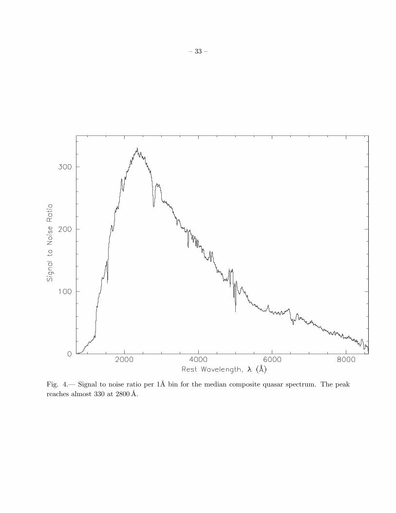
– 33 –

Fig. 4.— Signal to noise ratio per 1A bin for the median composite quasar spectrum. The peak

reaches almost 330 at 2800 A.

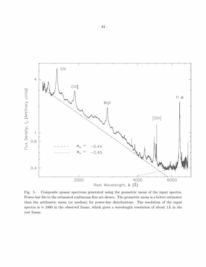
– 34 –

Fig. 5.— Composite quasar spectrum generated using the geometric mean of the input spectra.

Power-law fits to the estimated continuum flux are shown. The geometric mean is a better estimator

than the arithmetic mean (or median) for power-law distributions. The resolution of the input

spectra is ≈ 1800 in the observed frame, which gives a wavelength resolution of about 1A in the

rest frame.

– 35 –

Fig. 6.— Expanded view of median quasar composite on log-linear scale, with emission features

labeled by ion. Labels ending with a colon (:) are uncertain identifications. The two power-law

continuum fits are shown by dashed and dotted lines. The flux from 1600-3800 A is also composed

of heavily blended Fe ii and Fe iii lines, and Balmer continuum emission.

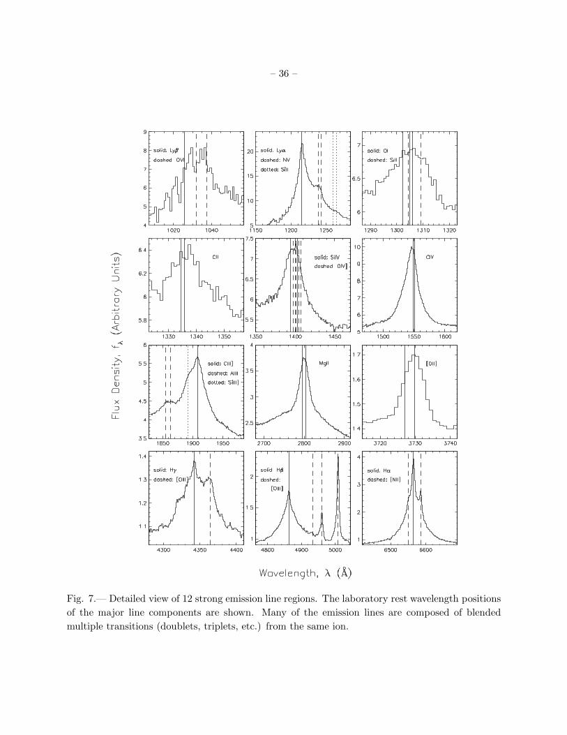
– 36 –

Fig. 7.— Detailed view of 12 strong emission line regions. The laboratory rest wavelength positions

of the major line components are shown. Many of the emission lines are composed of blended

multiple transitions (doublets, triplets, etc.) from the same ion.

– 37 –

Fig. 8.— Detailed view of absorption line regions in the low-redshift composite quasar spectrum

(solid line). The laboratory rest wavelength positions of detected absorption lines are labeled by

ion. Several strong emission lines are also labeled. The Ca iiλ3968 line is contaminated by emission

from [Ne iii]λ3967 and H ǫ. The full-sample composite spectrum (dashed line, offset) is also shown

for comparison in the top two panels (the spectra are identical in the wavelength region covered in

the bottom panel).

– 38 –

Fig. 9.— Emission line velocity offsets relative to laboratory rest wavelengths as a function of

ionization potential for selected emission lines. Error bars show the 1 standard deviation uncertainty

in the velocity measurement. The points are labeled by ion. Ionization potentials corresponding to

the same ion are slightly offset from each other for clarity. Permitted and semi-forbidden lines are

shown in the top panel, and forbidden lines are shown in the bottom panel.

– 39 –

Fig. 10.— Spectrum-to-spectrum variation of the quasar composite flux density relative to the

median flux as a function of rest wavelength.

– 40 –

Fig. 11.— Comparison of the SDSS median quasar composite spectrum (solid) with the LBQS

(dotted) and FBQS (dashed) composites. The spectra are scaled to the same average flux density

between 3020 and 3100A. Several major emission lines are labeled for reference.