
COMPOSITE AIRCRAFT COMPONENTS - Monash University
281
SQUEEZE FLOW DURING ASSEMBLY OF NOVEL JOINTS IN COMPOSITE AIRCRAFT COMPONENTS By Dipl.-Ing. Patryk Burka This thesis is submitted in fulfillment of the requirements for the degree of Doctor of Philosophy, Department of Mechanical & Aerospace Engineering Monash University December 2009
Transcript of COMPOSITE AIRCRAFT COMPONENTS - Monash University

SQUEEZE FLOW DURING ASSEMBLY OF NOVEL JOINTS IN
COMPOSITE AIRCRAFT COMPONENTS
By
Dipl.-Ing. Patryk Burka
This thesis is submitted in fulfillment of
the requirements for the degree of Doctor of Philosophy,
Department of Mechanical & Aerospace Engineering
Monash University
December 2009


Page i
Summary
An adhesive bonding process for composite spar-to-skin structures which can be found
in various aircraft components is proposed. In this process, referred to as the Insertion
Squeeze Flow (ISF) bonding process, a spar is inserted into a substructure which is
integrated into the composite skin. The cross-sectional shape of the substructure is similar
to the Greek letter π (Pi), the roof of the π being attached to the skin, and this substructure
is referred to as a Pi-slot. Before the insertion process is started, adhesive is placed into the
Pi-slot bottom and due to the insertion of the spar distributes into the gaps, or flow
channels, between the spar and the Pi-slot.
The adhesives that can be used for the conduction of the ISF processes were analysed in
order to develop an adhesive material model that can be used to represent the adhesive in
computational analysis. The adhesives Hysol EA 9395 and Hysol EA 9396 were selected
to be used for the ISF bonding process. A mixing ratio by weight of 70 – 30 EA 9395 to
EA 9396 was determined to have the lowest acceptable viscosity. The upper viscosity limit
was determined as the viscosity of EA 9395, which is the more viscous of the two
adhesives. Rheological tests showed that all studied adhesives are non-Newtonian, shear
thinning fluids. Furthermore, their time dependence appeared to be small and their
elasticity negligible. Constitutive material models (a Power law model and a five
parameter rational model) were derived based on shear viscosity versus shear strain rate
results.
In order to develop a two-dimensional (2D) numerical model for ISF using
computational fluid dynamics (CFD) software, a simplified ISF process was studied first.
A Newtonian fluid was specified as the fluid to be displaced by the insertion process and
numerical predictions were compared to the solutions of a derived analytical model for the
same problem setup, showing good agreement. To simulate the actual ISF bonding
process, the material models developed for the adhesives were implemented into this
numerical model. The agreement between experimental data and numerical predictions
was good.
ISF bonding processes conducted at constant insertion speed were studied numerically
applying the developed numerical 2D model. Insertion forces and pressures acting along
the Pi-slot walls were predicted and discussed for various insertion speeds, adhesive
viscosities, flow channel widths and insertion plate head designs. The main findings were a

Page ii
linear relationship between the insertion force and the insertion speed as well as a linear
relationship between the maximum pressure along the Pi-slot walls and the insertion speed.
The pressure was found to distribute approximately linearly along the Pi-slot wall, with a
maximum reached at the root of the Pi-slot wall. The ratio between the insertion force and
the maximum pressure was found to be independent of the insertion speed and the adhesive
viscosity. The established understanding of forces and pressures during ISF supports the
development of an ISF bonding process in terms of component design and in terms of
bonding facility design.
The effect of lateral misalignment was studied numerically in order to ensure complete
adhesive distribution during ISF. A dimensionless parameter ξ was defined referring the
wide to the narrow flow channel width and its effect on the adhesive distribution evaluated.
A second dimensionless parameter ψ was introduced which defines the ratio between the
flow front in the narrow and the flow front in the wide flow channel. One main finding of
this evaluation was that these two dimensionless parameters were found to be linearly
related with each other. Furthermore, it was found that this relationship was not affected by
the insertion speed, adhesive viscosity, initially applied adhesive volume and scarcely
affected by the insertion plate width variation. It was, however, affected by the shape of the
insertion plate head, with the rectangular head shape found to be the one most difficult to
fill. Procedures were proposed to ensure entire filling of the flow channels, consequently
leading to a desired Pi-joint quality, for this rectangular head shape.
Finally, the developed 2D numerical model was extended in regard to four aspects: the
consideration of the insertion control (at constant insertion speed or constant insertion
force), the consideration of a slight variation of the ISF process (ISF with adhesive pre-
application), the involvement of a fluid-structure-interaction (FSI) and finally the
consideration of ISF modelled three-dimensionally (3D). An ISF process conducted at
constant insertion force control was implemented into the numerical model and predictions
showed that relationships derived from constant insertion speed simulations were also
valid for constant force insertions. The effect of a FSI on the adhesive showed a negative
effect on the adhesive distribution compared to rigid Pi-slot walls, and two suggestions
were proposed to eliminate this effect in practice. Finally, three-dimensional (3D)
simulations were conducted to study the effect of a longitudinal misalignment. In the
considered range the adhesive flow was scarcely affected by this misalignment.
The detailed understanding of the adhesive flow during ISF is supportive for the design
of an adhesive bonding process that can be used to join spar-to-skin structures as found in

Page iii
aircraft components. The outcomes of the presented research work can be used as a guide
to ensure the joint quality of these spar-to-skin structures.

Page iv
Declaration of Originality
I, Patryk Burka, declare that this thesis contains no material which has been accepted for
the award of any other degree or diploma in any university or other institution.
To the best of my knowledge, this thesis contains no material previously published or
written by another person, except where due reference is made in the text of the thesis.
Patryk Burka, December 2009

Page v
Acknowledgements
I would like to thank the following people for their support during the conduction of this
work: first of all, my supervisors Professor John Sheridan and Professor Mark Thompson
and Dr. Xiaolin Liu, who have provided excellent continuous guidance throughout the
candidature.
Also, Dr. Duc At Nguyen and Dr. Peter Uhlher from the Chemical Engineering
Department at Monash University for their support during the rheological studies; John
Freeman and Rowan Paton from the CRC-ACS Ltd. during the conduction of experimental
studies; Dr. Llorenc Llopart Prieto, Anton Maier and Jochen Scholler from EADS MAS
for their input during my secondment to Munich; and Jane Moodie from the Faculty of
Engineering.
I would like to thank my parents and my brother, and last but not least my partner Leonie,
who has proven to be very patient during my candidature.
Further, thanks to my colleagues and friends, especially Joe Berry, Dr. Martin Griffith, Dr.
Justin Leontini, Dr. Hyeok Lee, Mehdi Nazarinia and Elham Tolouei, who all have
contributed in their own way to this work.
Finally, the financial assistance by the Department and the CRC-ACS Ltd. is also greatly
appreciated.

Page vi
Contents
Summary............................................................................................................................. i
Declaration of Originality................................................................................................ iv
Acknowledgements............................................................................................................ v
Contents............................................................................................................................. vi
List of Tables...................................................................................................................... x
List of Figures .................................................................................................................. xii
Abbreviations and Acronyms....................................................................................... xxii
Nomenclature................................................................................................................ xxiii
1 Introduction ............................................................................................................. 1
2 Literature Review .................................................................................................... 4
2.1 Techniques for Joining of Fibre-Reinforced Structures................................... 4
2.2 Adhesive Bonding of Fibre-Reinforced Structures.......................................... 7
2.2.1 Secondary bonding and co-curing...................................................... 7
2.2.2 Effects of joint designs and load cases............................................... 9
2.2.3 Spar-to-skin structures ..................................................................... 15
2.3 Adhesive Bonding using Pi-shaped Sub-Structures....................................... 20
2.4 Penetration and Squeeze Flows...................................................................... 28
2.4.1 Penetration flows.............................................................................. 28
2.4.2 Squeeze flows................................................................................... 33
2.5 Non-Newtonian Material Models .................................................................. 36
2.6 Summary ........................................................................................................ 42
3 Numerical and Experimental Method ................................................................. 43
3.1 Numerical Method ......................................................................................... 43

Page vii
3.2 Discretisation Schemes................................................................................... 46
3.2.1 Spatial discretisation......................................................................... 46
3.2.2 Temporal discretisation .................................................................... 47
3.3 Multiphase Flow, Non-Newtonian Fluids and Moving Boundaries .............. 48
3.3.1 Multiphase flow applying the Volume-of-Fluid method.................. 48
3.3.2 Non-Newtonian fluid viscosity......................................................... 50
3.3.3 Dynamic mesh model ....................................................................... 51
3.4 Validation ....................................................................................................... 54
3.4.1 Spinning bowl problem .................................................................... 54
3.4.2 Penetration flow in an open rectangular container ........................... 55
3.4.3 Domain size, resolution and mesh type independence..................... 59
3.4.4 Convergence ..................................................................................... 66
3.4.5 Time step tests .................................................................................. 67
3.5 Problem Setup and Post Processing ............................................................... 67
3.5.1 Problem setup ................................................................................... 68
3.5.2 Post processing ................................................................................. 71
3.5.3 Dimensionless parameters ................................................................ 74
3.6 Experimental Method..................................................................................... 75
3.6.1 Experimental equipment................................................................... 75
3.6.2 Dimensions of specimens, process parameter and materials............ 77
3.7 Summary ........................................................................................................ 79
4 Development of the Constitutive Adhesives Material Model............................. 80
4.1 Selection of Adhesives ................................................................................... 80
4.2 Methodology of Rheological Tests ................................................................ 81
4.3 Calibration and Validation of Equipment ...................................................... 86
4.4 Rheological Results........................................................................................ 91
4.4.1 Shear viscosity versus time .............................................................. 92
4.4.2 Shear viscosity versus shear rate ...................................................... 96
4.4.3 Time-dependence ........................................................................... 103
4.4.4 Viscoelastic properties.................................................................... 106

Page viii
4.4.5 Constitutive model development.................................................... 111
4.5 Summary ...................................................................................................... 114
5 Insertion Squeeze Flow at Constant Insertion Speed....................................... 115
5.1 Analytical and Numerical Solutions for Insertion Squeeze Flow with
Newtonian Fluids ................................................................................................... 115
5.2 Insertion Squeeze Flow at Low Insertion Speeds ........................................ 121
5.3 Insertion Squeeze Flow at High Insertion Speeds ....................................... 134
5.3.1 Results and discussion for insertion forces .................................... 134
5.3.2 Results and discussion for the Pi-slot wall pressure ...................... 137
5.3.3 Insertion force and Pi-slot wall pressure dependence .................... 140
5.3.4 Insertion force and Pi-slot wall pressure for different adhesive
material models ............................................................................................ 144
5.3.5 Effect of insertion speed on specific insertion force and Pi-slot
wall pressure ................................................................................................ 148
5.4 Insertion Squeeze Flow at High Insertion Speeds with Different Insertion
Head Shapes ........................................................................................................... 150
5.5 Experimental Study of ISF at High Insertion Speeds .................................. 155
5.6 Summary ...................................................................................................... 161
6 Insertion Squeeze Flow considering Lateral Misalignment............................. 162
6.1 Possible Misalignments during Insertion..................................................... 162
6.2 Causes of Lateral Misalignment .................................................................. 163
6.2.1 Manufacturing tolerances............................................................... 164
6.2.2 Spring-in effect............................................................................... 165
6.2.3 Process induced Pi-slot distortion .................................................. 166
6.3 Lateral Misalignment Effect on the Adhesive Flow .................................... 168
6.3.1 Results and discussion.................................................................... 169
6.3.2 Explanation of asymmetrical adhesive flow .................................. 186
6.3.3 Effect of different insertion head shapes........................................ 189
6.4 Mitigating the Effects of Lateral Misalignment........................................... 192

Page ix
6.4.1 Use of spacers................................................................................. 192
6.4.2 Bending forces on insertion plate due to spacers ........................... 195
6.5 Summary ...................................................................................................... 195
7 Extensions of the Numerical Model for Insertion Squeeze Flow..................... 197
7.1 Insertion Squeeze Flow at Constant Insertion Force.................................... 197
7.1.1 Introduction .................................................................................... 197
7.1.2 Numerical Method.......................................................................... 198
7.1.3 Results and discussion.................................................................... 200
7.2 Insertion Squeeze Flow with Adhesive Pre-Application ............................. 211
7.3 Insertion Squeeze Flow including Fluid-Structure Interaction .................... 214
7.3.1 Introduction .................................................................................... 214
7.3.2 Numerical method .......................................................................... 215
7.3.3 Results and discussion.................................................................... 219
7.4 3D Numerical Model for Insertion Squeeze Flow ....................................... 227
7.4.1 Problem setup ................................................................................. 227
7.4.2 Results and discussion.................................................................... 229
7.5 Summary ...................................................................................................... 231
8 Conclusions and Future Work............................................................................ 233
8.1 Conclusions .................................................................................................. 233
8.2 Future Work ................................................................................................. 236
References ...................................................................................................................... 239
Appendix A..................................................................................................................... 245
Appendix B..................................................................................................................... 248

Page x
List of Tables
Table 1: Advantages and disadvantages of mechanical fastening and adhesive bonding
as presented in Matthews (1987b)..................................................................... 5
Table 2: A summary of advantages and disadvantages enumerated for adhesive
bonding and co-curing of joints. ....................................................................... 9
Table 3: The dimensions of the I-beam components that were tested (Potter, 2001a). .... 17
Table 4: Force ratios derived for three models that describe the seating of a crown for
two different distances between the crown and the tooth (Cook, 1982). ........ 32
Table 5: Spring-damper models for the description of various polymer deformation
characteristics as described in Menges et al. (2002). ...................................... 38
Table 6: Comparison of calculated and numerically predicted insertion forces for
different density and viscosity ratios at various insertion speeds. .................. 58
Table 7: Drag coefficient variation for varying sizes of the outflow region..................... 60
Table 8: The effect of the grid resolution on the drag coefficient..................................... 63
Table 9: Mesh type independence analysis results............................................................ 65
Table 10: Effect of convergence criteria on the drag coefficient at the body. .................. 66
Table 11: Time step size effect on the solution................................................................. 67
Table 12: Test matrix for ISF experiments conducted at low insertion speed. ................. 78
Table 13: Specimen dimensions for the second row of ISF experiments. ........................ 79
Table 14: Investigated adhesive mixing ratios for determination of lowest ratio. ............ 81
Table 15: The shear viscosity of a cannon certified viscosity standard liquid silicone at
different temperatures as provided by the manufacturer................................. 87
Table 16: Apparent shear viscosities at different shear rates for two adhesive viscosity
ratios, indicating the deviation between two different measurements. ........... 90
Table 17: Comparison of shear indices that were determined for EA 9395 for four
different data sets. ........................................................................................... 91

Page xi
Table 18: Effect of the test type – either apparent or quasi-dynamic viscosity - on
shear viscosity data at three different shear rates. ........................................... 98
Table 19: Adhesive shear viscosities determined from apparent and quasi dynamic
tests at different shear rates for 70 – 30 weight percentage mixtures of
EA 9395 to EA 9396. .................................................................................... 101
Table 20: Adhesive shear viscosities determined from apparent and quasi dynamic
tests at different shear rates for 85 – 15 and 70 – 30 weight percent
mixtures of EA 9395 to EA 9396. ................................................................. 103
Table 21: Parameters for the five parameter rational model fit that are used to define
the adhesive mixtures viscosities................................................................... 114
Table 22: Nominal dimensions and baseline parameters applied for the first set of ISF
experiments.................................................................................................... 129
Table 23: Insertion speeds, adhesive viscosities and insertion plate widths for the
tested specimens in low insertion speed ISF experiments............................. 133
Table 24: Insertion force/maximum pressure – ratio for dimensionless times of 1 and
1.54 for different insertion speeds and adhesive shear viscosities. ............... 141
Table 25: Maximum pressure at Pi-slot walls for five parameter rational adhesive
viscosity models at t* = 1 for different adhesive viscosities and insertion
speeds............................................................................................................. 147
Table 26: Manufacturing tolerances as specified in the Mojo project (MoJo, 2007) and
the resulting flow channel widths.................................................................. 164
Table 27: Fill levels in the narrow and the wide flow channel for different ξ for
dimensionless times of 1 and 1.57................................................................. 173

Page xii
List of Figures
Figure 2-1: Different configurations of commonly used joint types (Hart-Smith, 1987). 10
Figure 2-2: The Pi-joint design is illustrated with different insertion head shapes........... 10
Figure 2-3: Typical shear and transverse tensile stress distribution in a double-lap
joint, as presented by Adams (Adams, 1986).................................................. 13
Figure 2-4: Steel-CFRP joints with varying taper-adhesive fillet combinations as
investigated by Adams (Adams, 1986). .......................................................... 14
Figure 2-5: I-beam design that was analysed in Potter et al. (2001a). .............................. 16
Figure 2-6: Tooling for the assembly of an I-beam using a secondary bonding
technique (Potter, 2001a). ............................................................................... 18
Figure 2-7: A Pi-joint assembly for structural connections as presented in
Kilwin (2006a); the Pi-joint contains the spar (1), the Pi-sub-structure (2),
the skin (3) and the adhesive (4). .................................................................... 24
Figure 2-8: Standoffs (3) to assure a minimum bond thickness in a Pi-joint, and self
locating features (1, 2) ensure the spar position in the joint (Kilwin, 2006a). 26
Figure 2-9: Schematic demonstration of a cylinder with radius Ri penetrating into a
Newtonian fluid contained in a vessel with radius ro (Malkin, 1994)............. 28
Figure 2-10: Idealized model used for the derivation of acting forces for the seating of
a crown in a cross-sectional view, studied in Cook (1982)............................. 30
Figure 2-11: Three models used to describe the problem of the seating of a crown by
Cook (1982): Parallel plate model (1), Pochettino geometry model (2,
cylindrical) and penetrometer geometry model (3, cylindrical)...................... 31
Figure 2-12: Typical stress-strain characteristic of a glassy polymer below the glass
transition temperature...................................................................................... 39
Figure 3-1: Two-dimensional illustration of a control volume. ........................................ 45
Figure 3-2: Log viscosity versus log shear rate plot for a shear thinning fluid................. 51
Figure 3-3: Penetration flow in a rectangular container analysed as a validation case
for the adhesive flow in ISF. ........................................................................... 56

Page xiii
Figure 3-4: Comparison between calculated and numerically predicted insertion force
with respect to flow time for an insertion speed of 5 mm/min and a constant
viscosity of 1000 Pas. ...................................................................................... 57
Figure 3-5: Typical mesh set-up and domain size used for the simulation of adhesive
flow in ISF bonding processes......................................................................... 59
Figure 3-6: Drag coefficient of insertion plate against element number indicating the
effect of grid resolution on the predictions...................................................... 62
Figure 3-7: Spatial resolution study for maximum applicable insertion speed and
adhesive viscosity. ........................................................................................... 64
Figure 3-8: Key dimensions for 2D flow simulations (schematic and corresponding
mesh). .............................................................................................................. 69
Figure 3-9: Mesh domain details indicating the moving boundaries and the necessary
interfaces between sliding elements. ............................................................... 70
Figure 3-10: Different insertion plate bottom shapes (also referred to as insertion head
shapes). ............................................................................................................ 71
Figure 3-11: Typical pressure-contour plot during ISF..................................................... 72
Figure 3-12: Pressure distribution at the slot wall for the above presented pressure-
contour plot...................................................................................................... 73
Figure 3-13: Phases distribution within the flow domain and a detailed interface of the
flowfronts (adhesive coloure red, air in blue).................................................. 74
Figure 3-14: Experimental test setup to measure the insertion force versus
displacement during an ISF bonding process. ................................................. 76
Figure 4-1: Test set-up and results for suitable weight percentage ratios of EA 9395 to
EA 9396........................................................................................................... 81
Figure 4-2: Cone and plate viscometer illustration of the equipment used for the
rheological tests. .............................................................................................. 83
Figure 4-3: Method of measurements for viscosity versus stepwise increasing shear
rate tests. .......................................................................................................... 84
Figure 4-4: Applied shear rate with respect to time graph for the thixotropic
measurements. ................................................................................................. 85

Page xiv
Figure 4-5: Shear viscosity of a calibration liquid with respect to time at a constant
shear rate of 1 s-1. ............................................................................................ 86
Figure 4-6: Polynomial fit of the calibration liquid viscosity versus temperature............ 87
Figure 4-7: Two apparent shear viscosity graphs as a function of time for EA 9395 at a
shear rate of 0.1 s-1. ......................................................................................... 92
Figure 4-8: Two apparent shear viscosity graphs as a function of time for EA 9395,
each at shear rates of 1 s-1 and 10 s-1. .............................................................. 94
Figure 4-9: Two apparent shear viscosity graphs as a function of time for a 70 – 30
weight percentage mixture between EA 9395 and EA 9396, each at shear
rates of 0.1 s-1 and 1 s-1.................................................................................... 95
Figure 4-10: Four data sets showing shear viscosity as a function of shear rate
measurements for 100% EA 9395................................................................... 96
Figure 4-11: Three data sets showing shear viscosity as a function of shear rate
measurements for 70 – 30 weigth percentage mixtures of EA 9395 to
EA 9396......................................................................................................... 100
Figure 4-12: Shear viscosity as a function of shear rate measurements from two data
sets for a 85 – 15 weigth percentage mixture of EA 9395 to EA 9396......... 102
Figure 4-13: Shear stress versus shear rate for a thixotropic loop test for 100%
EA 9395 (300 s loop). ................................................................................... 104
Figure 4-14: Shear stress versus shear rate for a thixotropic loop test for 100%
EA 9395 (20 s loop). ..................................................................................... 104
Figure 4-15: Thixotropic 300 s loop for a shear rate range from 0.1 to 10 s-1 for 100 %
EA 9395......................................................................................................... 105
Figure 4-16: Shear stress versus shear rate for a 20 s- and a 300 s-loop up to 10 s-1 for
an EA 9395 to EA 9396 mixing ratio of 70 – 30 by weight. ........................ 106
Figure 4-17: Storage and loss modulus versus strain at a frequency of 100 rad/s (100 –
0)................................................................................................................... 107
Figure 4-18: Storage and loss modulus versus strain at a frequency of 100 rad/s (70 –
30)................................................................................................................. 108

Page xv
Figure 4-19: Storage and loss modulus versus frequency for a constant strain of 0.5 %
for 100 % EA 9395........................................................................................ 109
Figure 4-20: Storage and loss modulus versus frequency for a constant strain of 1 %
for 100 % EA 9395........................................................................................ 109
Figure 4-21: Storage and loss modulus versus frequency for a constant strain of 1 %
(70-30). .......................................................................................................... 110
Figure 4-22: Power law viscosity fits for EA 9395 and mixtures of EA 9395 and
EA 9396......................................................................................................... 112
Figure 4-23: Five parameter rational model fit for all adhesives mixtures. .................... 113
Figure 5-1: Key dimensions for the analysis of insertion squeeze flow with a
Newtonian fluid. ............................................................................................ 115
Figure 5-2: Force balance between pressure and shear stress on an infinitesimally
small Newtonian fluid element (Schroeder, 2000). ....................................... 116
Figure 5-3: Numerically and analytically predicted insertion forces as a function of
dimensionless time for different insertion speeds for an ISF process with a
Newtonian fluid. ............................................................................................ 118
Figure 5-4: Numerically and analytically predicted insertion forces as a function of
dimensionless time for different fluid viscosities for an ISF process with a
Newtonian fluid. ............................................................................................ 119
Figure 5-5: Comparison of the velocity distribution with respect to flow channel
position predicted from the analytical and numerical models. ...................... 120
Figure 5-6: Numerically predicted shear rates in the adhesive within the flow channel
for insertion speeds of 2 and 10 mm/min. ..................................................... 122
Figure 5-7: Viscosity fields at t* = 0.21 at an insertion speed of 10 mm/min for a) a
70-30 weight percentage ratio of EA 9395 to EA 9396 and b) 100 %
EA 9395......................................................................................................... 123
Figure 5-8: Insertion force as a function of dimensionless time at different insertion
speeds for EA 9395........................................................................................ 125
Figure 5-9: Pressure contours at one specified dimensionless time of t* = 1.11 for an
insertion speed of 2.5 mm/min and EA 9395. ............................................... 126

Page xvi
Figure 5-10: Insertion force versus dimensionless time for different adhesive
viscosities at an insertion speed of 5 mm/min............................................... 127
Figure 5-11: Two insertion forces versus dimensionless time plots for vins = 5 mm/min
and ηadh = 70 – 30 as measured in the ISF experiments. ............................... 130
Figure 5-12: Comparison between measured and predicted insertion forces with
respect to insertion speed at t* = 1. ............................................................... 131
Figure 5-13: Comparison between measured and predicted insertion forces with
respect to adhesive viscosity at t* = 1. .......................................................... 132
Figure 5-14: Predicted transient insertion force and images of specified flow fronts at
three different times for baseline parameters. ............................................... 135
Figure 5-16: Predicted insertion forces versus dimensionless time for different
insertion speeds and adhesive viscosities...................................................... 136
Figure 5-17: Pressure distribution along the Pi-slot wall boundary for baseline
parameters at t*=0.89. ................................................................................... 138
Figure 5-18: Effect of insertion speeds and adhesive shear viscosities on transient
maximum Pi-slot wall pressure. .................................................................... 139
Figure 5-19: Effect of the insertion speed and the adhesive viscosity on the insertion
force/maximum Pi-slot wall pressure – ratio with respect to dimensionless
time................................................................................................................ 143
Figure 5-20: Effect of the adhesive material model on the predicted transient insertion
force for two adhesive viscosities. ................................................................ 145
Figure 5-21: Shear viscosity field at an insertion speed of 120 mm/min at t* = 0.21 for
a) the power law model and b) the five parameter rational model................ 146
Figure 5-22: Measured adhesive viscosity with respect to shear rate for three samples
of a 70 – 30 mix of EA 9395 to EA 9396. .................................................... 146
Figure 5-23: Effect of the adhesive viscosity (70-30 left, 100-0 right hand side) on the
insertion force/maximum Pi-slot wall pressure – ratio with respect to
dimensionless time, predicted applying the five parameter rational model. . 148
Figure 5-24: Insertion speed effect on a) specific insertion forces and b) maximum
pressures on the Pi-slot walls at t* = 1 and a 70 – 30 adhesive mix. ............ 149

Page xvii
Figure 5-25: Insertion head shape variations................................................................... 151
Figure 5-26: Predicted transient insertion force for different insertion head shapes....... 152
Figure 5-27: Initial adhesive distribution for the four investigated head shapes.
Adhesive is represented by the red colour, air is blue. .................................. 153
Figure 5-28: Transient maximum pressure along the Pi-slot wall with respect to
different insertion head shapes. ..................................................................... 154
Figure 5-29: Test setup for the second set of experiments to measure the insertion
force during an ISF bonding process. ............................................................ 156
Figure 5-30: Measured insertion forces plotted against dimensionless time for the
rounded and the tapered insertion plate heads in comparison to numerical
results for the same cases with a total flow channel width of 1 mm. ............ 157
Figure 5-31: A Pi-joint after bonded applying the ISF process at constant speed; three
spacers were used to align the insertion plate in the Pi-slot. ......................... 158
Figure 5-32: Numerically predicted insertion forces for a narrow and a wide total flow
channel width compared to experimentally measured insertion forces,
plotted with respect to dimensionless time for the tapered insertion head
shape. ............................................................................................................. 160
Figure 6-1: Possible misalignments that can occur during ISF: a) Lateral (x-axis) and
angular misalignment around z-axis; b) Angular misalignment around y-
axis; c) Angular misalignment around x-axis................................................ 162
Figure 6-2: Key dimensions that define the Pi-slot structure and that are specified in
the MoJo project (MoJo, 2007). .................................................................... 163
Figure 6-3: The permissible flatness deviation as defined in Mojo (2007)..................... 165
Figure 6-4: Two back-to-back flanged laminates approximating the Pi-slot for the
description of the spring-in effect (Liu, 2009). ............................................. 165
Figure 6-5: Lay-up of the Pi-slot; the fibre layers can be distinguished through the
different colours, and fibre-orientation is specified in the legend through
different line types. ........................................................................................ 166

Page xviii
Figure 6-6: Illustration of the Pi-slot wall deflection due to insertion pressure leading
to a broadening of the flow channel; the pressure is caused by the flow of
the adhesive. .................................................................................................. 167
Figure 6-7: Beam model to approximate the Pi-slot wall deflection; boundary
conditions at the bottom of the Pi-slot is fixed into the wall as a cantilever. 168
Figure 6-8: Schematic illustration of lateral misalignment resulting in different flow
channel widths δ1 and δ2,, shown as a top- and a cross-sectional view......... 169
Figure 6-9: Numerically predicted fill heights with respect to dimensionless time for a
perfectly aligned insertion represented by 826 points within an interval of
1.6 dimensionless time units t*. .................................................................... 170
Figure 6-10: Numerically predicted fill heights in the narrow and the wide flow
channel with respect to dimensionless time for ξ = 1, ξ = 0.667 and ξ =
0.430. ............................................................................................................. 171
Figure 6-11: Numerically predicted fill heights with respect to dimensionless time in
the narrow flow channel for different ξ ratios............................................... 172
Figure 6-12: Numerically predicted flow front ratio ψ versus t* for different flow
channel width ratios ξ.................................................................................... 174
Figure 6-13: Relationship between the flow front ratio and the flow channel width
ratio derived from the numerical predictions. ............................................... 175
Figure 6-14: Flow front ratios for different flow channel width ratios after the adhesive
has reached the outflow in the wide flow channel. ....................................... 177
Figure 6-15: Relation between the flow front ratio and flow channel width ratio for a
specifed dimensionless time of t*=1.35. ....................................................... 178
Figure 6-16: Predicted fill heights with respect to dimensionless time in the wide and
narrow flow channel (ξ = 0.430) for two different insertion speeds and 70 –
30 weight percent EA 9395 to EA 9396. ...................................................... 179
Figure 6-17: Predicted fill heights with respect to dimensionless time in the wide and
narrow flow channel (ξ = 0.430) for two different adhesive viscosities at an
insertion speed of 60 mm/min. ...................................................................... 179

Page xix
Figure 6-18: Fill height as a function of dimensionless time in the narrow channel for a
ξ ratio of 0.430 for different initial adhesive amounts. ................................. 180
Figure 6-19: Definition of H0, total which is used for the second procedure to ensure
entire filling of the narrow flow channel in a misaligned insertion process.. 181
Figure 6-20: Effect of the total flow channel width on the fill height versus
dimensionless time for a) ξ = 0.667, b) ξ = 0.430, and c) ξ = 0.333. ............ 184
Figure 6-21: Flow channel width effect on the flow front ratio ψ, resulting from a
variation of the insertion plate width, plotted for three different flow
channel width ratios ξ. ................................................................................... 185
Figure 6-22: Static pressure distribution within the flow domain for t*=0.28 for a
perfectly aligned insertion of a) ξ = 1 and a laterally misaligned insertion
defined by b) ξ = 0.430.................................................................................. 186
Figure 6-23: Streamlines implying the flow of the adhesive for a misaligned insertion
defined by ξ = 0.430 at t* = 0.28. .................................................................. 187
Figure 6-24: Pressure distribution along the insertion plate bottom for differently
misaligned cases for t*=0.28. ........................................................................ 188
Figure 6-25: Pressure gradients along the insertion plate bottom for different
misaligned cases for t*=0.28. ........................................................................ 189
Figure 6-26: Transient fill height in the wide (W) and narrow (N) flow channels for
different insertion head shapes. ..................................................................... 190
Figure 6-27: Flow front ratios for different head shapes for a misaligned insertion
defined by ξ =0.667. ...................................................................................... 191
Figure 6-28: Variables defining the dimensions of the insertion plate............................ 193
Figure 6-29: Circularly bended insertion plate before and after restrained by spacers... 194
Figure 6-30: Geometrical relations for estimating the number of spacers (not to scale).194
Figure 6-31: A simple supported beam model applied for the calculation of the
bending force that acts at the insertion plate due to spacers.......................... 195
Figure 7-1: Schematic problem set-up and definition of parameters for the force
balance. .......................................................................................................... 198

Page xx
Figure 7-2: Block diagram showing the interaction between the constant force UDF
and the Fluent software. ................................................................................ 200
Figure 7-3: Insertion plate velocity as a function of the insertion plate position for a
constant force of 3000 N/m. The crosses show results from constant speed
tests when the insertion force is equal to 3000 N/m. .................................... 201
Figure 7-4: Insertion force versus insertion plate position for an insertion speed of
30 mm/s. ........................................................................................................ 202
Figure 7-5: Insertion plate speed plotted against dimensionless time for a constant
force insertion at 3000 N/m........................................................................... 203
Figure 7-6: Drag force on the insertion plate with respect to dimensionless time shown
by the solid line. The pressure acting at the Pi-slot walls (dotted line) with
respect to dimensionless time is also shown. ................................................ 204
Figure 7-7: Displacement of the insertion plate from its original position plotted
against process time for different applied forces........................................... 207
Figure 7-8: Adhesive flow comparison between a misaligned and a perfectly aligned
constant force ISF process............................................................................. 208
Figure 7-9: Flow front ratio as a function of dimensionless time (ξ=0.667). ................. 209
Figure 7-10: Initial adhesive distribution including pre-applied adhesive on the
insertion plate side walls. Blue shows the initial location of the adhesive. .. 213
Figure 7-11: Comparison of fill heights for a pre-applied and a standard ISF bonding
process as a function of dimensionless time. The pre-applied variant was
conducted with two and with three phases, which are presented by the
dotted lines. ................................................................................................... 214
Figure 7-12: Schematic of the actual and assumed pressure distribution along the Pi-
slot wall. This pressure results from the adhesive flow which is also shown
in the figure for one examplary time. ............................................................ 216
Figure 7-13: Illustrated simplification of Pi-slot wall as a cantilever beam;
representation of the deflection of the beam due to the acting pressure. ...... 217

Page xxi
Figure 7-14: Flow chart for updating the Pi-slot wall boundary nodes based on the
adhesive flow front position and pressure distribution along the Pi-slot
walls............................................................................................................... 218
Figure 7-15: Mesh set-up for the FSI simulations; the rightmost image emphasizes the
Pi-slot- and insertion plate-boundaries. ......................................................... 219
Figure 7-16: Pi-slot wall top distortion due to the adhesive flow for baseline
parameters...................................................................................................... 220
Figure 7-17: A comparison between the distortion of the left and the right Pi-slot wall
for baseline parameters. ................................................................................. 222
Figure 7-18: Pi-slot distortion as a function of dimensionless time for different
composite stiffnesses and adhesive viscosities.............................................. 223
Figure 7-19: Insertion force as a function of dimensionless time for different Pi-slot
wall stiffnesses and adhesive viscosities. ...................................................... 224
Figure 7-20: Transient fill height for an aligned and a misaligned FSI simulation......... 225
Figure 7-21: The effect of flexible vs. rigid boundary conditions on fill
heights (ξ=0.667). .......................................................................................... 226
Figure 7-22: Flow domains for 3D ISF simulations........................................................ 227
Figure 7-23: Illustration of misalignment around the y-axis as analysed in the 3D ISF
simulations..................................................................................................... 228
Figure 7-24: Adhesive distribution (shown as red) for an aligned symmetrical 3D ISF
simulation; the rest of the flow domain is filled with air (in blue). ............... 229
Figure 7-25: Adhesive fill height versus dimensionless time for a longitudinally
misaligned insertion plate. ............................................................................. 230

Page xxii
Abbreviations and Acronyms
AFRL/ML Air Force Research Laboratory and Manufacturing Directory
BC boundary condition
CAI Composite Affordability Initiative
CCD charged couple device (camera)
CFD computational fluid dynamics
CFL Courant-Lewy
CFRP carbon-fibre-reinforced plastics
CPU computer processing unit
EWI Edison Welding Institute
FEA finite element analysis
FEM finite element modelling
FRP fibre-reinforced polymers
FSI fluid structure interaction
ISF insertion squeeze flow
LCD liquid crystal display
MBM modified Bautisto-Manero (model)
MOJO Modular Joints for Composite Aircraft Structures
MTI mouldable thermoplastic interface
NCF non crimp fabric
NDT non-destructive testing
RAM random access memory
VARTM vacuum assisted resin transfer moulding

Page xxiii
Nomenclature
A shear viscosity extrapolated to zero shear rate
a half insertion plate width
a thermal diffusivity
b half Pi-slot width
c flow front
cD drag coefficient
cN flow front (narrow channel)
cW flow front (wide channel)l
D drag force
DP rate of plastic shape change
E Youngs (in-plane) modulus
e error
F bending force
F insertion force
F tensile loading
Fc constant insertion force
Ff acting shear forces
Fp pressure force
FτW wall shear force
h distance between tooth and crown

Page xxiv
h* remaining possible insertion plate displacement
H height of a layer within the gap between cylinder and vessel
H height of insertion plate
H* fill height
H0 initial adhesive height
H0,stop entire possible insertion plate displacement
H1 Pi-slot height
H1* non-dimensionalised Pi-slot height
I Moment of inertia
K consistency factor
k Boltzman constant
L insertion plate length
L overlap length
Lspacer distance between spacers
l distance between cylinder and vessel bottom
l distance between insertion plate and Pi-slot bottom
M bending moment
N narrow (flow channel)
N normalized deviatoric portion of the driving stress state
n Power law index
p pressure

Page xxv
Ri inner radius of vessel,
Ro outer radius of cylinder
T* stress state
t Pi-slot wall thickness
t time
U insertion speed (in analytic model)
vc (r) velocity distribution in flow between cylinder and vessel walls
vi insertion velocity
vins insertion speed
w Pi-joint length
W wide (flow channel)
W insertion plate width
α volume fraction
Δ circular bended insertion plate distance before spacers
δ circular bended insertion plate distance after spacers
δ distance between cylinder and vessel walls
δ flow channel width
γ& shear rate
η shear viscosity
θ temperature
κ1 Newtonian shear viscosity

Page xxvi
κ2 non-Newtonian shear viscosity
ξ flow channel width ratio
ρ density
σPM lowest principal stress
σTM transverse stress
τ shear stress
τ0 Yield stress
φ any physical quantity, e.g. p, u, v, w
ψ flow front ratio
ω net angle of rotation between initial and activated configuration of
thermal diffusivity

Page 1
1 Introduction
Much research has focussed on adhesive bonding of composite components for various
applications in the past two decades. This stems from the substitution of conventionally
used metals with composite materials in many applications due to their superior specific
mechanical properties, so that costs can be lowered and weight saved. Due to these benefits
the use of composites for aircraft components is of major interest and has led to an
increased use.
Various bonding techniques to join the composite components have been used.
Conventional bonding of metal components was achieved through mechanical fastening
such as riveting, screwing or bolting, and past research has enumerated the disadvantages
of these techniques if they are applied for composite materials. For the joining of
composite components adhesive bonding, though, offers great potential since it is
considered as a more fibre-friendly bonding method, lacking stress concentration around
holes as required for mechanical fastening, and is also considered to reduce weight.
However, there has not been enough research on the quality adhesive bonding to substitute
mechanical bonding entirely. Hence, adhesive bonding is not applied as the only bonding
method, but supported through mechanical fastening techniques, hence eliminating
benefits gained from adhesive bonding. More research into adhesive bonding is thus
needed to ensure it guarantees equal joint qualities as those which are achievable with
mechanical fastening, so that the advantages through adhesive bonding can be realised.
A typical composite joint is a spar-to-skin application, which can be found in aircraft
doors, wings and flap track beams. Some research has been conducted to adhesively bond
spars to skins, applying different design approaches. All of these designs have been
considered as beneficial in cost and weight savings. One specific design, which uses a π-
shaped substructure that is attached to the skin, is additionally considered as being capable
of reducing undesired peel stresses. This substructure is referred to as Pi-slot. Its roof can
be co-cured or stitched to the skin, creating one component. The spar can then be inserted
into the Pi-slot and adhesively bonded to it, creating an adhesively bonded Pi-joint.
However, most studies of Pi-joint applications did not include any description of the
adhesive bonding techniques applied. Where adhesive bonding techniques were described,
they appeared to be quite complex. Furthermore, a number of the techniques could only be

Page 2
used with low viscous adhesives, while many adhesives are high viscous. Thus, a detailed
investigation of an alternative adhesive distribution technique is required.
This alternative adhesive distribution technique is referred to as an insertion squeeze
flow (ISF) bonding process. There are advantages of the ISF bonding process compared to
other adhesive distribution techniques described in the literature, of which the main are that
there is no restriction to the type of adhesive used and the simplicity of the setup of the ISF
process. In the proposed research study, an insertion squeeze flow (ISF) bonding process is
analysed. The adhesive is placed in the bottom of the Pi-slot and the spar (insertion plate)
is inserted into the Pi-slot, penetrating into the adhesive and displacing the adhesive into
the gaps, or flow channels, that are formed between the insertion plate and the Pi-slot.
Fully cured, an adhesive bond is formed between the insertion plate and the Pi-slot.
Research studies have investigated similar squeeze flow types, however, the investigated
geometries differed from the considered design and the displaced fluids varied from the
investigated adhesives.
The broad aim of the project is to study the adhesive flow during the ISF bonding
process and to use this understanding to enable the development of an ISF bonding process
for composite components. The study of adhesive flow is conducted analytically,
experimentally, and particularly numerically.
A specific aim of the project is to predict insertion forces acting during ISF and
pressures on the Pi-slot walls from the numerical analysis. An adhesive model developed
to represent the adhesive viscosity has to be implemented into the numerical model in
order to conduct the simulation of ISF. Knowledge of forces and pressures would be
supportive in designing an ISF bonding process. The predictions should be obtained for
ISF bonding processes conducted at constant speed and at constant force insertions.
Another specific aim of the project is to predict adhesive flow for misaligned insertions
in order to specifie tolerances and guidelines to ensure Pi-joint quality. Pi-joint quality
requires that the adhesive distributes evenly between the insertion plate (spar) and the Pi-
slot (skin plus substructure). Dimensionless parameters defining the adhesive distribution
have to be determined and their effect on the bonding quality evaluated.
Another specific aim is the consideration of how the Pi-slot wall stiffness affects the
adhesive distribution compared to the case if the Pi-slot walls are rigid. This includes the
incorporation of a fluid-structure-interaction (FSI) type of problem; the adhesive flow
implies a pressure on the Pi-slot walls, which may lead to a distortion of the Pi-slot walls,
which may in turn affect the adhesive flow.

Page 3
In this thesis, a comprehensive literature review relavant to the study is conducted in
Chapter 2. It includes the general consideration of conventional bonding and adhesive
bonding methods for composite structures, especially focussing on advantages and
disadvantages of those. Alternative bonding methods are introduced and reviewed,
followed by the consideration of Pi-joint application, especially the adhesive distribution
during the bonding process. Chapter 2 is concluded with the review of penetration and
squeeze flows, and with the presentation of proposed viscosity material models.
The numerical and experimental methodology is described in Chapter 3. The bulk of
Chapter 3 deals with the description of the computational method used for the development
of the numerical model. It also includes spatial and temporal resolution studies and the
two-dimensional (2D) set-up and definition of the problem.
In Chapter 4 the selected adhesives are described in detail and appropriate mixing ratios
determined. Results from various rheological tests are presented and the Chapter is
concluded with the proposition of two adhesive material models.
Chapter 5 reports a numerical study of ISF conducted at constant speed. Insertion forces
and Pi-slot wall pressures for ISF applying the adhesive material model are related to the
insertion speed and adhesive viscosities.
Chapter 6 reports on the effect of lateral misalignment on the adhesive distribution
during ISF obtained from numerical simulations. It outlines the effect of input variables as
insertion speed, adhesive viscosity, initially applied adhesive volume, total flow channel
width and insertion plate head design on the adhesive distribution in laterally misaligned
insertions.
In Chapter 7, the extension of the 2D numerical model for ISF is outlined. The
extensions are the simulation of an ISF bonding process conducted at constant insertion
force, the simulation of an ISF bonding process with pre-applied adhesive on the insertion
plate side walls, the simulation of a fluid-structure-interaction problem for ISF and finally
the three-dimensional (3D) consideration of ISF conducted at constant insertion speed.
Chapter 8 concludes the thesis and suggestions for future work are given.

Page 4
2 Literature Review
In Chapter 432H2, a broad discussion of some of the aspects that are potentially relevant to
insertion squeeze flow problems applied for adhesive bonding are examined. In
Section (433H2.1) different joining techniques for fibre-reinforced materials are introduced and
compared. Section 434H2.2 focuses on one particular bonding method, the adhesive bonding of
fibre-reinforced structures, and comparisons are made between two joining techniques,
which are the secondary bonding and the co-curing. Joint design analysis for adhesively
bonded joints is also presented within this section. Following, Section 435H2.3 details the
utilisation of Pi-shaped substructures in order to adhesively bond composite structures.
Then, in Section 436H2.4, penetration flows of Newtonian fluids are discussed first, followed by
discussion on squeeze flows of Newtonian and non-Newtonian fluids between two
approaching boundaries. Finally, material models developed for the characterisation of
rheological behaviour of non-Newtonian fluids are presented in Section 437H2.5.
2.1 Techniques for Joining of Fibre-Reinforced Structures
A good introduction into the topic of joining fibre-reinforced plastics is provided by
Matthews in “Joining Fibre-Reinforced Plastics” (Matthews, 1987a). Within this work,
joint designs for adhesive bonding and mechanical fastening are compared. Analytical and
finite element analysis methods for stress strain analysis of parts joined in both techniques
are presented and advantages and disadvantages of each technique are specified.
First, Matthews gives a brief introduction into joining techniques in general (Matthews,
1987b). It is stated that theoretically a structure is desired to lack any joints as those are
considered as a source of weakness and excess weight. Practically, though, limitations on
component size due to manufacturing processes, inspection requirements and accessibility,
repair, transportation and finally assembly mean that loaded joints are inevitable in large
structures.
Two techniques are generally applicable for joining fibre-reinforced plastics:
mechanical fastening and adhesive bonding. The advantages and disadvantages are
summarized in 438HTable 1 according to Matthews (1987b):

Page 5
Table 1: Advantages and disadvantages of mechanical fastening and adhesive bonding as
presented in Matthews (1987b).
+ -
Mechanically fastened joints − Disassembly possible
− No surface preparation
required
− Stress concentration at
holes
− Large weight due to
design requirements
and fasteners
− ‘Fibre-unfriendly’
method
Adhesively bonded joints − ‘Fibre-friendly’ method
and stress minimization
− Weight and cost-savings
− Disassembly
impossible
− Environmentally
effectible
− Complex inspection
methods
− Requires quality
assurance during
manufacturing
On the one hand, mechanical fastening of joints allows disassembly and does not
require surface preparation prior to joining. On the other hand, disadvantageous are stress
concentrations around the holes that are provided for fasteners. Due to design requirements
as a minimum thickness of the bonding partners and due to the fasteners’ weight, weight in
excess of the one expected for an adhesively bonded joint may be experienced. Adhesive
bonding, however, can be considered as a ‘fibre-friendly’ joining technique as fibres are
not damaged through the process of hole drilling. Disassembly of adhesively bonded joints
is not possible. Complex inspection methods may be prevented through quality assurance
during manufacturing of the bonding partners. Furthermore, joint strength may decrease
due to environmental effects.

Page 6
Considering mechanical fastening more in detail first, Collings (1987) provides a good
overview about common mechanical joining techniques. Mechanically fastened joints can
be subdivided due to the fastener that is implied. Screws, rivets and bolts have been
applied with varying success (Collings, 1987).
Self-tapping screws are considered as a simple and inexpensive connection but
accessibility of the reverse side of a joint is impossible. As thread stripping is likely, self-
trapping screws are not recommended where frequent demounting is required (Collings,
1987).
The use of rivets is suitable for laminate thicknesses of up to 3 mm (Collings, 1987).
Different types and forms are available, varying in being hollow or solid and for a range of
head and bolt types and sizes. The riveting process might cause damage to the laminate as
discussed by Matthews (Matthews, 1976), where an optimum level of constraint caused by
clamping is derived and suggested. In general, non-countersunk rivets are preferred to
countersunk ones (Matthews, 1980). Furthermore, the use of solid rivets compared to
hollow rivets results in stronger joints.
Finally, bolting is considered as the technique of choice in applications where
disassembly due to inspections and maintenance is required. Collings investigated a wide
range of variables as lay-up, fibre orientation and bolt diameter and stated bolted joints to
be the most efficient form of mechanical fastener (Collings, 1987).
An investigation of effects on mechanically fastened joint strengths always has to
consider failure modes (Collings, 1987, Matthews, 1987b). Collings (1987) enumerates
five different failure modes: tension, shear, bearing, cleavage and pull-out. The joint
strength of mechanically fastened composite joints can be affected by the fibre and matrix
material, lay-up, stacking sequence, fibre-orientation or hole and fastener
diameter (Collings, 1987, Matthews, 1987b).
Comparing the two bonding methods, there is a vital difference in the size of the
adherends whether the bonding method is mechanical fastening or adhesive bonding. A
mechanical fastener usually demands adherends of several millimetre thickness compared
to fractions of a millimetre for adherends that are bonded applying an adhesive (Matthews,
1987b). In case of adhesive bonding, the bonding mechanism is achieved through adhesion
between the adherends and the adhesive. Joint strength is affected by surface ply
orientation, stacking sequence, joint geometry, loading, matrix and adhesive material. In
many cases the matrix might be much weaker than the structural adhesive so that failure

Page 7
may occur through delamination or interplane fracture (Matthews, 1987b). Other failure
modes are listed and explained in sub-Section 439H2.2.2.
2.2 Adhesive Bonding of Fibre-Reinforced Structures
In this section, different adhesive bonding techniques for fibre-reinforced structures are
considered, which are the adhesive bonding (secondary bonding) and a technique referred
to as co-curing (primary bonding). The techniques are explained and compared with each
other. Also, work is presented that deals with stress analysis in secondary adhesively
bonded fibre-reinforced structures.
2.2.1 Secondary bonding and co-curing
Two methods to join composite structures are adhesive bonding and co-curing.
Adhesive bonding, on the one hand, is referred to as secondary bonding which means that
the bonding partners (adherends) are manufactured first and then bonded in a second
process step. During co-curing, on the other hand, the partners to be bonded are
manufactured and joined in-situ. The joint is formed during the composite curing process
of each component. This technique is referred to as primary bonding as no additional
process step is required. Advantages and disadvantages of primary and secondary bonding
are pointed out below.
Shin and Lee (2003) analysed the fatigue behaviour of double lap joints that were co-
cured for different bonding parameters such as surface roughness of the steel adherend and
stacking sequence of the composite adherend. They considered co-curing to be
advantageous compared to secondary bonding as the manufacturing process is simpler.
Curing and bonding is conducted at the same time and excessive matrix material from the
composite adherend functions as the adhesive (Shin, 2003).
In 2000, Shin, Lee and Lee studied the lap shear strength of a co-cured single lap joint
experimentally. Investigated parameters were bond length, surface roughness of the steel
adherend and stacking sequence of the composite adherend. The lap shear strength was
found to significantly be affected by the bond length and the stacking sequence of the
composite laminate. Surface treatment of the adherends, however, appeared to only
minorly affect the lap shear strength. In this paper, it was pointed out that co-curing is
considered as the most advantageous bonding method. This was based on two
comparisons: firstly, a comparison between mechanical fastening and adhesive bonding
supported the advantages proposed in the previous section, which are that there is no need

Page 8
for holes which lead to delamination, fibre cut and stress concentration around the holes,
and that adhesive bonding generates a larger stress bearing area, a uniform stress
distribution, superior resistance to fatigue or cyclic loads and an attractive strength to
weight ratio (Shin et al., 2000). Secondly, comparing primary and secondary bonding, Shin
et al. concluded that, due to the aspect that surface treatment only has a minor effect on the
lap shear strength of the composite adherends, and hence is not required for co-curing, but
for adhesive bonding, the most convenient joining method is co-curing.
However, several other authors considered secondary bonding to be advantageous to
primary bonding.
Work by Potter et al. in 2001 investigated adhesive crack propagation in bonded
joints (Potter, 2001b). Their scope was the establishing of a measure to control the progress
of cracks in adhesives in bonded joints. They selected paste adhesive instead of film
adhesive for two reasons: first, an adhesive bonding process can be applied – in contrast to
adhesive film bonding – without pressure. This allows bonding of complex geometry joints
and also is preferable when tight tolerances cannot be guaranteed. Second, paste adhesives
can accommodate incorporation of geometrical details such as reverse chamfers and
adhesive fillets. As shown by Adams (Adams, 1986), the level of induced through
thickness stresses can be reduced significantly when applying fillets and tapers at the edges
of the joint.
Matthews (1987), Liechti (1987), Adams (1987), and Potter et al. (2001) stated that the
tensile and shear stress distribution along a joint is not uniform. Moreover, it reaches
maximum values at the edges of the joint. Therefore, a design modification can improve
the joint strength significantly and is achievable in a simple way when using secondary
adhesive bonding.
A summary of advantages and disadvantages of both bonding techniques is given in
440HTable 2.

Page 9
Table 2: A summary of advantages and disadvantages enumerated for adhesive bonding
and co-curing of joints.
+ -
Adhesively bonded joints Pressure-free process
allows complex joint
designs
Incorporation of
geometrical details
Additional process
step
Surface
preparation
required
Complex
inspection
methods
Co-cured joints Simpler: curing and
bonding conducted
simultaneously
No surface
preparation required
Pressure required
during assembly
No geometrical
design freedom to
encounter against
non-uniform stress
distribution in
joints
It has been shown that both techniques bare advantages and disadvantages, and
depending on the structures to be bonded, the one might be more beneficial than the other.
In the presented study, secondary bonding was selected in particular due to the possibility
of joining complex structures without pressure (MoJo, 2006).
2.2.2 Effects of joint designs and load cases
In order to use adhesives for the bonding of composite materials the understanding of
joint design and loading type effects on the joint strength is substantial. Additionally,
failure modes have to be taken into consideration (Adams, 1986).
Joint designs and failure modes are introduced briefly below. Then, work on the stress-
strain characterization of joints is presented, including analytical and finite element
methods. Finally, the work by Adams et al. (1986) is discussed.

Page 10
Adhesively bonded joints are used in different configurations. Some of the most
common configurations are presented in 441HFigure 2-1:
1
2
3
4
5
6
7
8
9
Figure 2-1: Different configurations of commonly used joint types (Hart-Smith, 1987).
From 1 to 8, the joint types can be labelled as follows: bonded doubler (1), unsupported
single-lap joint (2), single-strap joint (3), tapered single-lap joint (4), double-lap joint (5),
double-strap joint (6), tapered strap joint (7), stepped-lap joint (8) and scarf joint (9).
Their relative usage can be placed in perspective by their bonded joint strength and
complexity of the joint, for example a complicated scarfed or stepped-lap joint is able to
transfer higher loads than rather simple single-lap or double-strap joints (Hart-Smith,
1987).
The joint that is considered in the presented work is a Pi-joint, which is presented
schematically in 442HFigure 2-2, illustrated with three alternative insertion plate head shape
designs.
Figure 2-2: The Pi-joint design is illustrated with different insertion head shapes.
None of the common used joint types agrees fully with the Pi-joint. Clearly, all single
joints differ significantly from the Pi-joint design. However, there are similarities between
the Pi-joint and the double joints as double-lap and double-strap joints, but also between
the Pi-joint and the stepped or scarf joint, because all of these designs are comprised of an
enveloping and a centre component. Hence, stress-strain analysis of these designs is

Page 11
considered beneficial for the stress-strain characterisation of Pi-joints. Investigations of the
joint design will take into account the bottom shape of the centre adherend of the Pi-joint,
as demonstrated in 443HFigure 2-2.
A brief description of failure modes for adhesively bonded joints is given next.
Strongest joints fail outside the joint area and show equal to the strength as the adherends.
The next highest strengths occur when the joint fails due to the shear strength of the
adhesive. Finally, the weakest failure mode is considered to be the one when the joint fails
by failure of the adhesive under peel loads (Hart-Smith, 1987). Therefore, peel stresses in
the adhesive should be avoided as far as possible. Hart-Smith (1987) suggests tapering to
be a good method to avoid peel stresses in the adhesive.
The stress-strain characteristic can be determined analytically and numerically through
finite element analysis (FEA) (Keller, 2005). FEA has the advantage of including specific
geometries and fillets, or anisotropy and non-linearity in material behaviour when
predicting joint strengths. It was shown that these features affect the joint strength
significantly (Adams, 1986).
In the literature both ways – analytical and FEA – were investigated frequently. Some
examples showing the development of analytical descriptions of stress-strain behaviour are
Volkersen’s shear lag analysis (Volkersen, 1938, Volkersen, 1965), which only takes shear
stresses into consideration and assumes the adherends to be absolutely rigid. This study
was extended by Goland and Reissner (1944) who took into account the resulting bending
moment in single lap joints. These bending moments cause stresses acting in the through
thickness direction and are referred to as peel stresses. Peel stress is the least desirable
stress in joints (MoJo, 2006, Russel, 2006). Volkersen (1965) considered bending effects
as he introduced a through thickness peel stress variable. Renton and Allaman included
bending, shear and normal stresses in their models (Renton, 1977), and Tsai et al. and Tsai
and Morton (Tsai, 1994, Tsai, 1998) showed that Oplinger’s method, who added the effect
of large deflection in the bonding area of single lap joints (Oplinger, 1994), is only valid
for thin and flexible adhesives.
FEA was investigated by Adams et al. (Adams, 1986), Adams (Adams, 1987), and
Richardson et al. (1993). Several other studies concentrated on the failure modes and crack
propagation in the adhesive (Hart-Smith, 1987, Hart-Smith, 2002, Potter, 2001b). The
scope of the presented study is not a stress-strain analysis, though, and therefore the
aforementioned papers are not reviewed in detail. However, the design of the joint is a
parameter that is modified in the presented investigation and as shown above affects the

Page 12
joint strength. Therefore, one particulat study, Adams et al. (1986), is considered in more
detail.
Adams et al. (1986) evaluated strengths of cabon-fibre-reinforced plastics (CFRP)/steel
double-lap joints loaded in tension. According to Adams et al. (1986), adhesive bonding is
a most attractive method for joining carbon fibre reinforced plastics (CFRP) for many
reasons. When compared to optional bonding techniques as riveting and bolting, the main
advantages adhesive bonding offers are improved fatigue resistance, the possibility to
disregard a minimum sheet thickness required for bolting and riveting and greater design
flexibility (Adams, 1986). To fully utilise these advantages, a proper understanding of
various design parameters which affect the strength of adhesively bonded joints is
necessary. Among others, their main aims were “i) to analyse the stress distributions in the
joints, […], iv) to use these studies to optimise the design of the joint in order to attain a
significantly increased failure strength”, p. 30, ll. 11-14. These aspects are important for
the conducted research for a number of reasons: firstly, when considering the effects of
insertion plate head shape on the adhesive distribution within the Pi-joint, the choice of the
head shape design should be made regarding the effect of design on the joint strength.
Secondly, the resulting distance between the bonding partners in the bottom area of the Pi-
joint is considered. And thirdly, the adhesive fillet design at the top of the Pi-slot should be
created according to the outcomes presented in Adams (1986).
It is expected and found that a double-lap joint does not fail by shear but by tensile
loading. In 444HFigure 2-3 the shear and transverse tensile stress distribution along the overlap
length L in an adhesive layer are considered (Adams, 1986).

Page 13
Region of elasticdeformation
Region of plasticdeformation
Region of plasticdeformation
Yield stress ofadhesive
Shear stress distributionin adhesiveτ
σt
Transverse tensile (normal) stressdistribution in the adhesive
-
+
0
0 L
L
Figure 2-3: Typical shear and transverse tensile stress distribution in a double-lap joint,
as presented by Adams (Adams, 1986).
The shear stress distribution shows a constant yield stress of adhesive in the region of
plastic deformation at the edges of the overlap length. An elastic deformation region is
found in between. The transverse tensile stress distribution shows maximum values at the
edges of the overlap length, which, if possible, should be avoided.
Several joint designs were investigated by Adams et al. (1986) to avoid these maxima.
The designs were modified by locally changing the geometry in the regions where the
maximum loads occur. Special attention was given to the shape of the fillet and the
tapering of the adherend edges. 445HFigure 2-4 shows the designs that were investigated, with
design 1 being the top one and design 5 being the one on the bottom.

Page 14
Steel Adhesive CFRP
Basic design
Outside taper
Inside taper
Adhesive fillet
Inside taper and adhesive fillet
Figure 2-4: Steel-CFRP joints with varying taper-adhesive fillet combinations as
investigated by Adams (Adams, 1986).
A finite element analysis (FEA) of the effect of the tensile stresses normal to the loading
direction was conducted in both the CFRP inner adherend and in the adhesive layer.
Details about methodology of the FEA can be found in Adams et al. (1986). The maximum
transverse stresses σtm in the CFRP occurred in the region adjacent to the edges of the outer
steel adherends, as expected. Essentially, the use of a taper only as in the designs 2 and 3
shows a minor effect on the maximum transvers stresses σtm (Adams, 1986). However,
comparing the transverse stress distribution between designs 1 (basic design) and
design 5 (inside taper and adhesive fillet) showed that the stress concentration could be
reduced from a maximum of σtm = 35 MPa for design 1 to a maximum of σtm = 6 MPa for
design 5, which is a reduction of 83 % (Adams, 1986).
An analysis of the principal stress distribution σpm in the adhesive layer for different
designs underlines the effect that the use of an adhesive fillet combined with an inner taper
in the steel adherends also provided the best results, meaning lowest principle stress
maxima σpm. The principal stress maximum can be reduced from σpm = 101 Mpa for
design 1 to σpm = 28.9 Mpa for design 5.
The comparison between experiment and theory shows that in all experimental cases the
mode of failure was not due to a shear failure of the adhesive but was due to interlaminar

Page 15
fracture of the inner CFRP. More specifically, the interlaminar fracture occurred at the
region of the overlap length where the steel outer adherends terminated. This failure is
obviously caused by the transverse tensile stresses in the joint. It was found that two
possible failure mechanisms could account for the interlaminar fracture; either transverse
tensile stresses at the edge of the joint close to the interface in the CFRP or concentrations
of principal stresses in the adhesive resulting in yielding and straining to failure under
predominantly tensile forces. The latter might lead to interlaminar failure as well as cracks
would run through the adhesive to the interface of the CFRP. Considering those two failure
mechanisms is important when considering the theoretical predictions as the predictions
would be different depending on the assumed failure mechanism.
Essentially important for the presented research work is the effect the inside taper and
the adhesive fillet have on the failure load. Failure load significantly increased when an
inside taper was applied and combined with an adhesive fillet (design 5). This was
observed for both the experimental results and the theoretical predictions. These results
will be taken into consideration when the effects of designs of the head shape on the
adhesive flow are studied.
2.2.3 Spar-to-skin structures
An adhesive bonding application for a spar to skin composite structure is presented in
the following. A summary of the work is conducted and comparisons are drawn to the Pi-
joint design that will be investigated in the presented study.
In 2001, Potter et al. (Potter, 2001a) investigated adhesive bonding in secondarily
bonded I-beam composite structures. The work was carried out as part of the IMI
programme ‘Innovative Approaches to Composite Structures’ and was contributed to by
Bristol University, BAE Systems, Airbus, Ltd Filton (BAE), and Cranfield University.
Aim of the programme was the demonstration of ‘feasibility of utilising bonded
construction in heavily loaded composite structures’ (Potter, 2001a). Potter enumerates
various advantages that justify their investigation on adhesive bonding, being reduced parts
count compared to mechanical fastening and minimising necessity of drilling or machining
of components (Potter, 2001a). The I-beam test piece was intended to represent a wing skin
and spar in the wing box of a commercial jetliner. Details of ultimate shear flows and shear
stresses that had to be carried by the test piece can be found in Potter et al. (2001a). After
design, manufacture and testing in three-point and four-point bending a post-test evaluation

Page 16
was conducted to obtain an understanding of the bondline quality and to identify the cause
of failure.
The I-beam design is shown as a cross-section in 446HFigure 2-5.
Skin (flange)
Corner piece (L)
Adhesive
Spar (web)
Figure 2-5: I-beam design that was analysed in Potter et al. (2001a).
The design represents two T-joints where the middle I-beam is chosen as the spar within
a wing box and the top and bottom parts represent the skin. The modules are considered to
be bonded secondarily meaning that they are manufactured first and than adhesively
bonded. The separate corner pieces are to strengthen the skin-to-spar-joint and to allow
tolerances in the spar height and the skin thickness. Dimensions of the test piece are
summarized in 447HTable 3 and were determined by means of scaling.

Page 17
Table 3: The dimensions of the I-beam components that were tested (Potter, 2001a).
Component Length [mm]
Spar depth 150
Skin width 150
Skin thickness 10
Spar thickness 8
Overall length 2000
For further details about choice of lay-up design it is referred to Potter et al. (2001a). A
more detailed description about the application of the finite element analysis (FEA)
method used for determination of the joint design can be found there as well. The
methodology provided investigates design freedoms as overlap length and geometry of the
ends of the joints, development of the three dimensional analysis using a linear elastic
model, and three-dimensional analysis including non-linearity and non-linear adhesive
properties.
The manufacturing of the I-beam joint is described in the following. All components
used were manufactured using prepreg lay up and autoclave technology. On all surfaces
peel ply was used to minimise surface contamination. Furthermore, all bonding surfaces
were manually grid blasted. Although a cabinet grid blasting model generally would
provide a more even activated bonding surface, the manual option was chosen to simulate
the manufacturing according to the feasibility of utilising it for large scale components.
A tooling system had to be developed for the adhesive bonding process. The system
should generate the desired adhesive bondline thicknesses without use of spacers. The
developed tooling system used is illustrated in 448HFigure 2-6.

Page 18
1 2
Figure 2-6: Tooling for the assembly of an I-beam using a secondary bonding
technique (Potter, 2001a).
After coating part 1 with mould release and setting it on a bench horizontally, adhesive
is applied to the first pair of corner pieces. The adhesive is applied on the side facing the
spar and the corner pieces are set into place on the tooling side part 1. Then, adhesive is
applied on one side of the spar and the spar is lowered on the corner pieces afterwards.
Once in place, adhesive is distributed on the other side of the spar which is facing up. The
second pair of corner pieces is prepared with further adhesive and placed with its other side
on part 2 of the tooling system. Part 2 including corner pieces is then brought into correct
register with part 1, squeezing out excessive adhesive during this process. Next, skins are
prepared with adhesive and set on the corner pieces. Once in place, skin clamps are
tightened up until the skins sit in the correct position of the set up. Finally, the set up is
placed in an oven and the adhesive is cured according to the manufacturer’s cure schedule.
This assembly procedure provides possibilities of air entrapment and appears quite
complicated. This is confirmed by comments about the assembly found in the article: ‘The
assembly tooling was rather clumsy in use and would not be suitable for much larger
structures, but did allow a series of beams to be manufactured to consistent dimensions’,
ll. 29-32, page 394, Potter et al. (2001a). Incompletely formed fillets and voids in the

Page 19
adhesive fillets were exhibited in the first test specimen. In latter specimens (2, 3 and 4),
improved quality was achieved and ultrasonic non destructive testing (NDT) showed no
major defects.
For details about the testing procedure it is referred to Potter et al. (2001a) again. In
terms of testing results, the three-point bending test specimens failed at 77% of the
predicted load with a scatter of less than 1% of mean strength. The failure load was well
above the design ultimate required (123%). Sample 4 was tested in four-point bending and
failed at approximately 105% of prediction which was according to 165% of design
ultimate load.
Post-test evaluation included video tape evidence, acoustic emission evidence and strain
gauge evidence. Furthermore, an inspection of the failed surfaces followed attempting to
determine the bondline quality and final failure source.
The test specimens were essentially in three pieces, the tensile surface and the left and
right half of the rest of the I-beam. Each halve consisted of the spar, the compression
surface and the corner pieces. For an understanding of the causes of failure, the midpoint
of the detached tensile skin is the main feature of interest. The rest of the detached tensile
skin is separated via delamination in the skin. At the midpoint, though, the separation is
within the corner pieces and through the adhesive. This was considered as the initial point
of failure. Cracks propagated from the corner pieces through the adhesive and into the
tensile skin, resulting in delamination within the tensile skin and leading to separation
between the tensile skin and the rest of the beam.
Marks left from the edge of the spar on the adhesive layer indicate the weak bonding at
this point. According to Potter et al. (2001a), the bond between the spar and the adhesive
must be regarded as of reduced strength. Furthermore, there are areas on the corner pieces
showing little or no adhesion at all. Especially some beams show large voids within the
adhesive bond line which cover several cm2 in some cases.
In the discussion, it is mentioned that the preparation of large areas for bonding by hand
is very difficult. Despite the limitations of the test assemblies the performance of the beam
specimens was very good, exceeding all requirements comfortably.
Comparing Adam’s work with the presented research, similarities exist as both studies
deal with applications of adhesive bonding for spar-to-skin structures. The difficulties
experienced with the method proposed in Potter et al. (2001a) are considered to lay in the
assembly of the I-beam and in the preparation of large areas for bonding. The cause of
failure was seen to be in the rather weak adhesion between the spar and the adhesive and

Page 20
some areas of the corner pieces showed large void areas. The present study might
contribute to the improvement of spar to skin bonding quality. A different adhesive
bonding technique is investigated being insertion squeeze flow (ISF) bonding, where the
bonding partners are designed in a different way. Less air entrapment during the bonding
process is expected as air is expected to be pushed out of the bonding area in front of the
adhesive flow front. The ISF technique is also believed to provide a simpler assembly as
less modules are involved. The Pi-joint legs fulfil a similar function as the corner pieces in
the I-joint. Both constrain the middle structure and are bonded to it. The roof of the Pi-joint
is attached to the skin through stitching and co-curing so that the Pi-joint is already
integrated. A T-shaped structure is then achieved when the I-shaped counterpart is inserted
into the Pi-joint.
2.3 Adhesive Bonding using Pi-shaped Sub-Structures
Pi-joints – the name originating from the similarity to the Greek letter П – have been
used in various projects and applications involving adhesive bonding before. Some of these
applications are summarized below, presenting what was investigated and which results
were obtained. Furthermore, it reviews those applications and provides comparisons to the
presented research work.
A relatively early example where a Pi-joint design was applied for the bonding of
composite structures for aircraft components can be found in Wong (1992). Wong (1992)
presents the development of sandwich constructions for the all-composite aircraft
“Starship” by the Beech Aircraft Company, Wichita, Kansas. Examples for sandwich
construction components are the main wing, forward wing, pressure vertical stabilizer and
the control surfaces (Wong, 1992).
It is said that the main wing is a typical low part count bonded structure. The sandwich
skins are manufactured first as a one piece cure each, the lower skin having a stiffener
assembled into it. Adhesive and scrim cloth is applied into the upper skin which is than
lowered into the lower skin, creating a bond with the stiffener. Wong (1992) states that the
“key to be successful of this assembly technique is Beech patented 3 dimensional woven
fibre joint[s],” ll. 7-8, page 2. Bonding is realized by utilising a cure paste adhesive. Beside
the low part count approach advantages are seen in the elimination of peel stresses.
Further low part count structures are the forward wing and the pressure cabin. The
forward wing is a structure including two spars and its assembly is completed in a single
cure cycle. The spars are held in position through silicon rubber bags inside each wing box

Page 21
cell while the upper and lower skins are held in a matched female tool. Bonding is realized
through co-curing. The pressure cabin consists of a left and right pre-cured half that are
bonded together through the utilisation of hot temperature paste adhesive.
In September 2005 the revision of a Navy ManTech program was published that
summarized some results from a research program titled “Aircraft Primary Structure
Adhesive Bonding Development” (Navy, 2005). Participants of the program were the
Edison Welding Institute (EWI), Lockheed Martin Aeronautical Systems, Boeing
Integrated Defense Systems and NAVAIR. In the problem description and objectives the
potential of adhesive bonding for primary structures is pointed out first: significant cost
and weight savings. However, the difficulties in the controllability of manufacturing
tolerances lead to a lack of confidence in fulfilling Navy Aircraft service requirements,
resulting in an avoiding of adhesive bonding usage. Bonded-bolted designs are used
instead. The objective of the Navy ManTech program was the investigation of effects of
defects and of manufacturing process variability with the purpose of improving
producibilty and reliability of adhesive bonded joints.
Studied process variables were “influences of nominal differences in materials, Pi-joint
design variations, assembly and bonding process variations such as adhesive thickness,
web offset, poor offset condition, improper cure and joint porosity,” ll. 22-26, (Navy,
2005). The results were obtained from testing over 800 specimens and these data were
transferred to the Navy/Air Force and Composite Affordability Initiative (CAI), another
program investigating the application of adhesive bonding for composite primary aircraft
structures that is discussed below.
The revision considers the Navy ManTech program of being a technical success. It is
stated that the applicability of adhesive bonded primary structures is seen for fixed-wing
aircraft programs. Lockheed Martin used results from the program for the design of the
Joint Strike Force (JSF) inlet duct. Benefits resulting from this application are stated to be
$200,000 cost and 80 lbs weight savings. Further applications of improved adhesive
bonding are for existing co-bonded structures and in repair. Summing up, additional
benefits are a 95% reduction of mechanical fasteners for the example of the JSF duct and
an improved aerodynamic and signature performance, leading to a more robust and
efficient aircraft.
The aforementioned Composite Affordability Initiative (CAI) program is presented
next. Russel (2006) summarizes the contents and achievements of the CAI. Motivation for
the program was due to the fact that despite the potential of composites for weight

Page 22
reduction in aircraft “the aircraft industry was reluctant to implement them in new
aircraft”, ll. 8-9, Russel (2006). Perceived risks and barriers for the implementation of
advanced composites in aircraft had to be addressed. Participants of this eleven-year effort
were the Air Force Research Laboratory Materials and Manufacturing
Directorate (AFRL/ML) and Air Vehicles Directorate, the Office of Naval Research-
ManTech, Bell Helicopter Textron, The Boeing Company, Lockheed Martin Corporation,
and Northrop Grumman Corporation. It is said that to afford the integration of advanced
composites in aircraft the assembly costs had to be cut. The most suitable way to do so was
considered in minimizing the number of thousands of parts and hundreds of thousands of
fasteners, as this would make drilling holes and installing fasteners unnecessary. Thus, a
major source of labour and rework in aircraft structures would be avoided. Part integration
and structural assembly through bonding were chosen to track the problem. The objective
of the CAI is formulated as “to ‘establish the confidence to fly large integrated and bonded
structures’”, ll. 31-32, page 1, Russel (2006).
The primary technology for the manufacturing of integrated composite structures was
vacuum assisted resin transfer moulding (VARTM). In this technology, vacuum is applied
to suck the liquid resin into a cavity where the composite preform has been placed before.
The main advantages towards state-of-art manufacturing processes are the abandonment of
an autoclave leading to reduced capital equipment costs. The second main advantage is
seen in the VARTM resins which cure at lower temperatures. This enables the use of more
inexpensive tooling reducing system development costs. Several parts were demonstrated
and showed fibre-volumes and per ply thickness comparable to autoclave cured parts.
VARTM was considered to be a production process ready for aerospace industry (Russel,
2006).
Of greater importance for the conducted research work is the consideration of the
bonding process involved in the CAI. Pi-joint bonded primary structure design was chosen
as the bonding technique for large integrated structures. The reluctant use of adhesive
bonding for primary structures is said to be based on concerns about the judge ability of
bond quality. For example, they stated that the distinguishing between a joint where the
adhesive is properly distributed and a joint where the bonding partners are in touch with
each other without adhesive between them (kissing joint) is difficult to achieve. However,
Russel points out the benefits for a proper designed and processed adhesive joint to be
what was stated by several other publications, the reduced part and fastener count and
reduced assembly times.

Page 23
The bonded joint design of choice was the Pi-joint (π-joint). The roof of the Pi (π) can
be co-cured or co-bonded to the skin. Acting as a stiffener the Pi-joint provides benefits in
terms of structural redundancy and is said to be stronger than a double-lap joint.
Furthermore reduced assembly times are achieved through the providing of a determinate
assembly feature. It is stated that in typical skin and spar bonding processes adhesive out
times are experienced. The distribution of the adhesive in the clevis of the Pi-joint is
expected to take significantly less time which means out times are avoided. Furthermore
adhesive areas exposed to air are smaller for the Pi-joint. The paper gives no information
about the way the adhesive is distributed between the adherends within the Pi-joint.
Coupons to full scale testings proved the Pi-joints’ robust and predictable performance.
One key finding was that the adhesively bonded Pi-joints strength was three to five times
higher than the strength of the part of the Pi-joint that was co-cured to the skin.
Consequently, the Pi-joint is not considered to be the weak link in the primary structure.
Pi-joints with defects as thick bondlines, canted blades, blades skewed to one side of the
clevis, voids and peel plies that were not removed prior to bonding still performed well.
Tested applications were the X-45A wing carry through and the X-45C wing to design
limit load, design ultimate load and finally to failure. According to Russel (2006) “these
structural and ballistic test show that bonded structures can meet structural requirements
for military aircraft”, ll. 38-41, page 3, Russel (2006). Assembly times could be reduced
from 50 – 80% depending on the structure, and cost savings ranged from 20 – 50%.
Within the project, the development of key supporting tools and technologies was also
considered. For example computational tools allowing more accurate analysis taking into
account peel as well as shear stresses, damage progression evaluation tools, non-
destructive testing for production and maintenance and certification approaches were
amongst those. For more details it is referred to Russel (2006).
Summing up, Russel considers the CAI to be a “huge technical success”, ll. 73-74,
page 4, Russel (2006). He states that “technology applications are increasing and are
anticipated to continue to expand”, ll. 78-79, page 4, Russel (2006). No information could
be found investigating the adhesive distribution in the Pi-joint. It is not clear if the adhesive
bonding process was conducted using the insertion squeeze flow method that is
investigated within the presented research work. Even if the insertion squeeze flow method
was applied in the CAI no publishing could be found. Thus, investigations on insertion
squeeze flow bonding of composite structures appear to be meaningful and of major

Page 24
importance, especially considering the huge potential it offers for composite structure
applications in aircrafts according to Russel (2006).
A very similar publication dealing with the Composite Affordability Initiative was
Russel (2007). Basically, the same approach and results are presented (Russel, 2007).
An article by Ritter published in July 2005 (Ritter, 2005) summarizes the outcomes of
the previously discussed works, which were the Navy ManTech program (Navy, 2005) and
the Composite Affordability Initiative (Russel, 2006). In general, it states that adhesive
bonding was investigated for applications in primary aircraft structures. It repeats the main
benefits gained from adhesive bonding compared to the use of mechanical fastening. No
additional information is published compared to the prior discussed works.
The Patent Application Publication “Minimum Bond Thickness Assembly Feature
Assurance” presents a feature to assure minimum bond thickness for a Pi-joint (Kilwin,
2006a). It is said that Pi-joint assemblies are becoming more prevalent for the assembly of
two structures especially if one or both structures are made of composites. Using this
assembly may provide a way to reduce weight of the structure and may provide an
increased structural strength.
The Pi-joint assembly is shown in 449HFigure 2-7.
1
2
4
3
Figure 2-7: A Pi-joint assembly for structural connections as presented in Kilwin (2006a);
the Pi-joint contains the spar (1), the Pi-sub-structure (2), the skin (3) and the
adhesive (4).
It consists of a spar (1), the Pi-member (2) and the skin (3). To connect the spar with the
Pi-member an adhesive (4) is filled in the gap between the spar and the Pi-member. A

Page 25
disadvantage is seen, however, in the complicated alignment between the Pi-member and
the spar prior to filling the gaps with adhesive.
According to Kilwin (2006a), there is a known process to align the parts by the use of
holes that are drilled into the parts. This is done when the parts are assembled, then the
parts are disassembled to remove any drill lubricant, chips and other foreign matter
introduced into the part during the drilling process. Afterwards the parts are assembled
again using fasteners to hold them in place to each other. Shims or wires can be used to
generate a minimum bondline thickness. These shims or wires are removed after the
adhesive starts to set and the so created voids are filled with additional adhesive. In ll. 62-
67, page 1, Kilwin (2006a), Kilwin et al. state that “[t]he additional steps of locating,
drillilng, cleaning, reassembly, fastening, shimming, unfastening, unshimming, and filling
voids […] are termed ‘waste’ which may be disadvantageous because time and money are
lost due to the additional albeit necessary steps for the present method of assembly.” To
avoid this “waste”, Kilwin states that an improved assembly method is required, a
reduction of the tooling during the assembly, and an elimination of the usage of shims and
wires.
Lean manufacturing concepts are introduced to identify a way to eliminate “waste”. It is
built on two fundamental principles being the elimination of waste and the accelerating of
the process. It is stated that this “attempt is to eliminate all activities that do not add to the
value of the assembly or the process”, ll. 87-88, page 1, Kilwin (2006a). After a process is
fully understood it is possible to improve and optimize it in order to increase its efficiency,
for example through simplifications of the design or standardization of the assembly
processes.
One concept that is briefly announced for an improved locating and aligning of the Pi-
assembly members is the use of a snap joint technology. This technology provides a robust
way to position and align several structures with each other. No details are given about this
technology.
It follows the description of the invention. The “minimum bond thickness assurance
feature for a Pi-joint assembly” allows the spar and the Pi-member to be self located. A
thickness control between the bonding partners is provided through “standoffs” that are
machined in the part that is inserted into the Pi-member. Optionally, self locating features
may be used together with the standoffs providing “horizontal control, vertical control,
alignment control, depth control, or edge control,” ll. 1-2, page 2, Kilwin (2006a). 450HFigure

Page 26
2-8 presents a minimum bond thickness assurance feature and a self locating feature,
respectively.
2
13
Figure 2-8: Standoffs (3) to assure a minimum bond thickness in a Pi-joint, and self
locating features (1, 2) ensure the spar position in the joint (Kilwin, 2006a).
A patent from 2006 presents an adhesive injection process for Pi-joint assemblies for
composite structures (Kilwin, 2006b). In this process a vacuum is created to distribute the
adhesive in the gaps. The steps involved in the presented patent start with the drilling of at
least two holes into the Pi-leg. Those holes act as ports for a vacuum that is applied to
distribute the adhesive between the bonding partners. Filler has to be inserted into the gap
between the female (Pi-member) and the male (spar/web) part and a sealant is applied
above the filler. After the set up is finished, a vacuum is created at one port and the
adhesive is injected into the other port as it is drawn into the gap towards the first port. In
background descriptions of Kilwin (2006b), alternative methods are described for the
adhesive distribution within the male and female part and their disadvantages are
explained. One alternative is the “plunge method” where the Pi-member is filled with the
adhesive. The spar is than plunged into the pool of adhesive. Kilwin (2006b) mentions
disadvantages of the plunge method in the control of spill over so that excessive adhesive
needs to be removed and the joint cleaned. The relative positioning between the parts is
seen as a second disadvantage.

Page 27
An alternative state-of-art method is the tube withdrawal method. A tube is placed in the
bottom of the female part and the male part is positioned above the tube. All openings
except for the opening where the tube will be withdrawn are closed via tapes. The adhesive
is inserted into the gaps through the tube while this is removed within a certain time frame
from the gap. Problems are seen in the appropriate speed of the withdrawal of the tube
which might either lead to voids and air pockets if the withdrawal is to fast or to spilling of
the adhesive if the withdrawal is to slow. Removal of the tape before setting of the
adhesive starts is mentioned as another difficulty.
The last alternative filling method is an injection method that uses one drilled hole as a
port to inject the adhesive into the gaps. To avoid spill out of the adhesive all openings are
closed with tape. As the pressure applied to push the adhesive into the gaps has to be quite
large depending on the viscosity and the gap dimensions, the tape is difficult to be kept in
place. This would lead to spill out resulting in need for cleaning. It is also stated that ports
are needed about every 12 in depending on the adhesive properties and the gap.
The adhesive injection process for Pi-joint assemblies is described as providing
increased productivity for Pi-joint assemblies.
The method of choice for the presented investigation is similar to the one described in
Kilwin (2006b) as plunge method. Although disadvantages are considered in the spilling
out of the adhesive resulting in a necessary cleaning, this can as well be considered as an
advantage as a proper fillet, which could be created through an appropriate removal of the
outspilled adhesive, can provide additional strength to the bonded joint (Adams, 1987,
Hart-Smith, 1987, Potter, 2001a, Potter, 2001b). The second disadvantage mentioned,
which was the relative positioning of the spar and the Pi-structure, is subject of analysis in
the presented research.
The adhesive injection process as presented in Kilwin (2006b) for Pi-joint assembly is
considered to have some disadvantages, one being the restrictions of the adhesive that can
be applied because its viscosity must be low so that it can be distributed through the
applied vacuum. This restriction is not expected in the investigated insertion squeeze flow
bonding process. According to the lean technology the drilling of holes into the Pi-legs can
be considered as waste of time and waste of money as the holes do not contribute in any
way to the Pi-joint. Lastly, it appears that the assembly steps involved in the ISF are less
complicated and less preparation is required compared to the adhesive injection process.
Main process steps in the ISF bonding process involve the filling of the Pi-member bottom
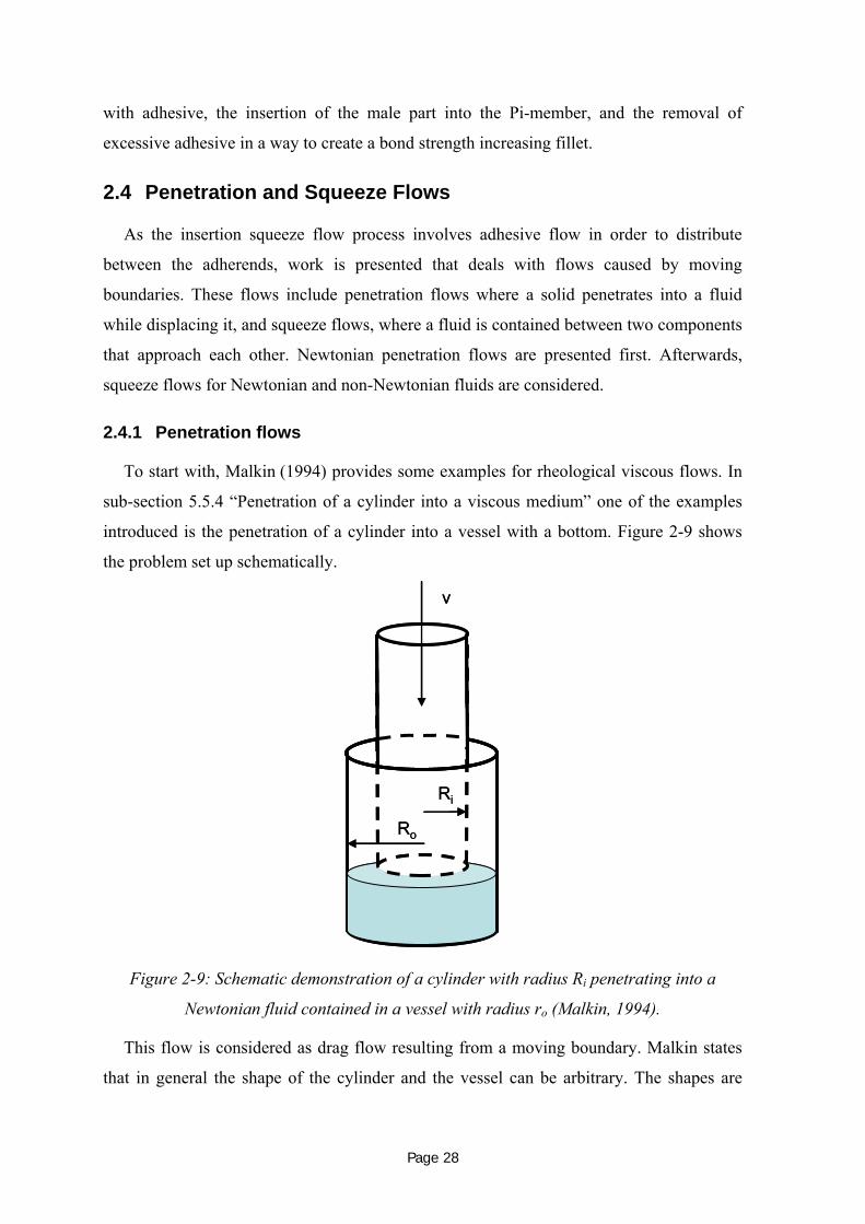
Page 28
with adhesive, the insertion of the male part into the Pi-member, and the removal of
excessive adhesive in a way to create a bond strength increasing fillet.
2.4 Penetration and Squeeze Flows
As the insertion squeeze flow process involves adhesive flow in order to distribute
between the adherends, work is presented that deals with flows caused by moving
boundaries. These flows include penetration flows where a solid penetrates into a fluid
while displacing it, and squeeze flows, where a fluid is contained between two components
that approach each other. Newtonian penetration flows are presented first. Afterwards,
squeeze flows for Newtonian and non-Newtonian fluids are considered.
2.4.1 Penetration flows
To start with, Malkin (1994) provides some examples for rheological viscous flows. In
sub-section 5.5.4 “Penetration of a cylinder into a viscous medium” one of the examples
introduced is the penetration of a cylinder into a vessel with a bottom. 451HFigure 2-9 shows
the problem set up schematically.
v
Ri
Ro
v
Ri
Ro
Figure 2-9: Schematic demonstration of a cylinder with radius Ri penetrating into a
Newtonian fluid contained in a vessel with radius ro (Malkin, 1994).
This flow is considered as drag flow resulting from a moving boundary. Malkin states
that in general the shape of the cylinder and the vessel can be arbitrary. The shapes are

Page 29
determined by the cylinder radius Ri(z) and the vessel radius R0(z) where the z-axis is the
axis of the cylinder and vessel.
One main parameter of interest is determined to be the resistance force that has to be
applied in order to push the cylinder into the viscous fluid. The resistance force consists of
two components: the force due to viscous friction along the sides of the cylinder and the
force due to the pressure that acts at the bottom of it. In case Ri(z) is not constant, and the
cylinder is shaped in a way that it consists of a flat and a tapered region, the pressure force
consists of two parts: the force acting on the tapered areas, which is termed Fp,1,and the
force acting on the flat bottom, termed Fp,2.
If the gap between the cylinder and the vessel is small, the flow can be treated as one-
dimensional (1D). When a constant velocity is applied on the cylinder, at an initial state it
starts to touch the liquid and penetrate into it, forcing some liquid to be displaced into the
gap. H is specified as the variable height of a displaced fluid layer within the gap and l is
variable distance between the cylinder bottom and the bottom of the vessel, both being a
function of time.
According to Malkin (1994) information on resistance force can be found by knowing
the pressure and velocity distribution. An analytical solution for a Newtonian Fluid is
presented. A Newtonian fluid is characterized through a proportional shear stress - shear
rate behaviour. For a non-Newtonian fluid, however, the shear stress varies with shear rate
nonlinearly. More detail about Newtonian and non-Newtonian fluids is given in
Section 2.5. The velocity distribution in the flow between cylinders is known
through (Malkin 1994):
⎟⎟⎟⎟
⎠
⎞
⎜⎜⎜⎜
⎝
⎛ −−
∂∂
+−=
0
20
0
2
2
0
0
ln
lnln
41
ln
ln)(
RR
RrRR
rRr
zp
RR
Rr
vrvi
ii
iz η
(2-1)
The pressure gradient has to be found and substituted into equation 452H(2-1). The shear
stresses at the solid surface can be found from equation 453H(2-2):
rvz
∂∂
=ησ (2-2)
The solutions for the acting shear force Ff and the two parts of the acting pressure forces
Fp,1 and Fp,2 can be found on pages 158-159 in Malkin (1994). Those solutions can be
simplified when assuming a small distance δ between the cylinder and vessel walls. For a

Page 30
cylinder with constant radius Ri(z) = R penetrating into a cylindrical vessel, the following
equation for the resistance force is derived (Malkin, 1994):
⎟⎟⎠
⎞⎜⎜⎝
⎛+= 3
34 623
δπη HR
lRvF (2-3)
Within the brackets, the first term represents the viscous forces and the second term
represents the pressure forces. It is a reasonable assumption that viscous forces are small
compared to pressure forces (Malkin, 1994). In comparison to Malkin’s work, the main
differences to the here presented research are that the fluid that is displaced is non-
Newtonian and that the geometry used is, considering a cross-section, a rectangular plate
and a rectangular container.
A similar problem was investigated by Cook (1982). For the process of the seating of a
dental crown, different filling materials were investigated and shear rates and acting forces
were calculated. As the chosen materials are non-Newtonian but can be considered
Newtonian for small shear rates, Newtonian governing equations were used for the
modelling of the flow problem. The seating of a crown is shown schematically in 455HFigure
2-10,
h
b
crown
tooth
h
b
crown
tooth
Figure 2-10: Idealized model used for the derivation of acting forces for the seating of a
crown in a cross-sectional view, studied in Cook (1982)
where h is the transient distance between the tooth and the crown, and b defines the
smallest radius of the crown which is found at its bottom.
Cook separates the problem into three models referring to different flow processes.
These models are shown in 454HFigure 2-11.

Page 31
F, v
h
2a
(1)
F, v
2a
2b
c
(2)
F, v
c2a
2b
(3)
F, v
h
2a
(1)
F, v
2a
2b
c
(2)
F, v
c2a
2b
(3)
Figure 2-11: Three models used to describe the problem of the seating of a crown by
Cook (1982): Parallel plate model (1), Pochettino geometry model (2, cylindrical) and
penetrometer geometry model (3, cylindrical).
The parallel plate model (1) represents the flow of the fluid out of the occlusal area
which is referred to as squeeze flow. The Pochettino geometry model (2) describes fluid
flow between two cylindrical walls. Finally, the penetrometer geometry model (3) is a
combination of (1) and (2), representing most authentically what happens in terms of fluid
motion, shear rates and acting forces. Subdividing the flow problem as stated above
allowed an interpretation of the relative magnitude of the acting forces. Cook (1982)
derived equations from Oka (Oka, 1960) and Smith et al. (Smith et al., 1948) to calculate
the acting forces due to the fluid motion for each model as shown in 456Figure 2-11 and
compared these. The force equations and forces for the different models for two different
distances h are presented in 457HTable 4.

Page 32
Table 4: Force ratios derived for three models that describe the seating of a crown for two
different distances between the crown and the tooth (Cook, 1982).
Model Force equation h=1 mm h=0.01 mm
Parallel plate geometry 3
4
1 23
hVaF ηπ
= 5.0 x 10⁻⁴ 4.0 x 10⁻⁸
Pochettino geometry
]ln)[(
42
⎟⎠⎞
⎜⎝⎛+
=
abab
VcaF ηπ 9.0 x 10⁻⁴ 8.0 x 10⁻³
Penetrometer geometry
])()([ln
2
22
223
abab
ab
VcF
+−
−⎟⎠⎞
⎜⎝⎛
=ηπ
1 1
Cook (1982) concludes from these results that the major forces acting during the seating
of a crown are due to the flow from the occlusal area into the gap between the walls.
Finally, Smith et al. (1948) investigated a rod moving axially into a fluid in a closed
tube. Cook’s and Oka’s equations describing the penetration flow are based on Smith’s et
al. (1948) derivations. Acting forces during the rising of the fluid between the walls of the
rod and the closed tube were derived. Starting from the general integral form of the
velocity distribution in Poiseuille flow, the velocity was determined to be defined as
BrL
AL
prV ++−
= ln24
2
πηη. (2-4)
Within equation 458H(2-4) V is the axial velocity of the displaced liquid that is flowing up
between the walls, p is the pressure acting within the liquid below the rod, r is the radius at
which the velocity is determined and finally L is the length between the bottom of the rod
and the maximum height of the displaced liquid (also refered to as flow front). A and B are
integration constants which result from the double integration of the balanced force
equation between the viscous and pressure forces, and can be determined from boundary
conditions.
The pressure term can be derived applying the continuity equation as the amount of
displaced liquid below the rod has to match the rising liquid 459H(2-5):

Page 33
∫=a
i
r
rii drrvrv ππ 22 (2-5)
Solving the integral and rearranging, the pressure term is derived as:
)()ln()(
42222
iai
aia
i
rrrrrr
Lvp
−−+=
η (2-6)
It is assumed that the resistance force is made up of two components, similar to the
approach applied by Malkin (1994), which are the shear forces on the side walls of the
cylinder and the pressure forces on the bottom of the cylinder. This can be expressed as
prrVLrF i
rri
i
22 πηπ +⎟⎠⎞
⎜⎝⎛∂∂
==
. (2-7)
Substitution of the three unknown variables (A, B and p) into equation 460H(2-7) gives the
following equation for the resisting force:
( )( ) ( ) ⎟⎟
⎠
⎞⎜⎜⎝
⎛+
⎟⎟⎠
⎞⎜⎜⎝
⎛⎥⎦
⎤⎢⎣
⎡−−⎟⎟
⎠
⎞⎜⎜⎝
⎛−
−=
i
a
i
i
aia
i
aia
iai
rrLV
rr
rrrr
rr
rrLVF
ln
2
lnln
2
2222
22 πηπη
(2-8)
From this equation, it can be seen that the force necessary for a rising of the fluid is a
linear function of the insertion velocity Vi of the rod, the viscosity η of the fluid and the
flow front L (Smith et al., 1948). Furthermore, the force is the sum of two terms which
represent the viscous and the pressure forces.
2.4.2 Squeeze flows
Many studies have investigated squeeze flows of various fluid types that are enclosed
between two parallel approaching discs or plates. Studied variables were material
properties, boundary conditions, dimensions and process parameters.
Adams et al. (Adams et al., 1997) presented a finite element solution for an elasto-
viscoplastic material that is squeezed between two approaching plates. No-slip and
lubricated wall boundary conditions were considered, with a Coulombic boundary
condition for the latter. Fluids exhibiting apparent yield behaviour as pastes or
concentrated suspensions were focussed on. For those fluids the constitutive material
behaviour is commonly described by one-dimensional forms of the Bingham or Herschel-

Page 34
Bulkey relationships (Herschel, 1926). However, for more complex flows as the
investigated squeeze flows inconsistencies in the flow field are experienced. Therefore,
Adams et al. (1997a) suggested the usage of a von Mises yield criterion combined with a
linear elastic response and a post-yield viscoplastic constitutive relationship. Experiments
were used to validate the finite element solution and good agreement was found for
compression forces, radial displacement fields and wall normal and shear stress
distributions.
Laun et al. (Laun, 1999) investigated squeeze flows of viscous fluids between parallel
approaching plates for a Newtonian and a power-law fluid. Their objective was to establish
a relationship between the squeeze force and the squeezing speed for partial slip boundary
conditions. The slip velocity is increasing linearly with increasing radius of the parallel
plates reaching a rim slip velocity at the edges of the plates. A procedure is proposed to
determine the rim slip velocity from squeeze flow experiments when a constant rim shear
stress is imposed. This procedure is based on derivations describing the relation between
squeezing speed and force. The derivation is conducted in two steps; the derivation for the
Newtonian material and small gaps is presented first, then the derivation for the power law
fluid is presented. According to Laun et al. (1999) partial slip occurs due to the presence of
a thin lubrication layer near the wall.
Newtonian fluids and Non-Newtonian soft solids were investigated experimentally in
(Meeten, 2004) while being squeezed between two parallel glass plates, with the motion
realised through the application of a constant force. For plate roughnesses varying between
0.3 and 31 μm the separation h(t) and the squeeze rate V(t) were measured. Non-
Newtonian soft solids showed boundary-slip being decreased or removed if plate
roughness was increased towards the upper range. Even with optically polished plates no
perfect slip could be achieved. According to Meeten (2004), a perfect slip boundary
condition can be described as an equibiaxial extensional strain on the material. This allows
measurement of the extensional rheology of a material. For a no-slip case, however, the
material squeezed suffers from an extensional and a shear strain. For R >> h and sufficient
boundary friction, the extensional contribution to the squeeze force is negligible (Meeten,
2002, Meeten, 2004).
Jackson et al. (2006) investigate squeeze flow between two approaching plates in order
to analyse a process called “mouldable thermoplastic interface” (MTI) which was
developed at the CRC-ACS Ltd., Fishermen’s Bend, Australia. MTI is described as a
manufacturing process with the purpose of locally altering dimensions of composite

Page 35
components (Jackson, 2006). It involves the co-curing of a thermoplastic layer on the
laminate and can be used for profiling, tolerancing or locating other components. During
the MTI process the thermoplastic material is squeezed between the approaching plates so
that some material flows out of the approaching area. To determine the final thickness of
the thermoplastic layer between the approaching plates, a flow model is derived from the
lubrication theory by Scott (1931). It is essential to know the viscosity to predict the final
thickness. However, consecutive viscosity measurements in a temperature range from 180-
200°C did not provide a repeatable result and the viscosity varied between 20,000 and
100,000 Pa.s. Those test showed a shear thinning fluid characteristic with increasing shear
rate, which was found to be approximatable by a power-law relation. Ultimately, the
viscosity was determined from squeeze flow tests when a pressure was applied and the
displacement of the plates was measured for isothermal conditions. This test allowed a
determination of the viscosity values which then were used to calculate the final thickness
with respect to various MTI process parameters.
Finally, an example using computational fluid dynamics (CFD) for the analysis of
squeeze flows was discussed by Mannan et al. (Mannan, 1995). An analytical and a CFD
model was developed to analyse the bonding of liquid crystal display (LCD) chips on glass
substrates. Particular interest was given to the establishing of dependences between applied
pressure, temperature, adhesive viscosity, and process time. When the pressure is applied,
the adhesive flows out of the bonding area while excessive adhesive is squeezed out,
similar to processes described above. The process is conducted isothermally near the
melting temperature of the thermoplastic adhesive. Several rheological properties had to be
determined in order to predict the process time. Viscosity and temperature versus shear rate
measurements were conducted as well as relaxation time tests to predict viscoelasticity. A
power law relation was found to best represent the adhesives shear thinning fluid
characteristics. The relaxation time was determined and was significantly smaller than the
expected process time. In this case – according to Leider (1974) – viscoelasticity can be
assumed to be negligible (Leider, 1974). To predict the motion of the plates as a function
of time analytically, the Scott equation was applied (Scott, 1931). The analytical
predictions varied from those predicted by the commercial finite element CFD code
FIDAP. Main reason for this discrepancy were found to be due to the different shapes of
the plates, as in the analytical case rounded plates were assumed and in the numerical case
the predictions were for square chips.

Page 36
2.5 Non-Newtonian Material Models
In the following section publications are presented that developed constitutive models
for the description of Non-Newtonian materials.
An introduction into the topic of flow of polymers is given in Chapter 5 of Menges et
al. (Menges, 2002). This Chapter deals with the flow of melted polymers which are
considered to be high-viscous fluids. The flow characteristics of high-viscous fluids are
governed by their stress-strain behaviour. Two types of deformations are
distinguished (Menges, 2002): shear deformation and strain deformation. Another
important property of melted polymers is viscoelasticity. A viscoelastic material is
characterized through its delayed stress release. Its behaviour is described as a mixture
between an elastic solid and a viscous fluid.
During polymer manufacturing processes a polymer melt typically experiences shear
deformations (Menges, 2002). This results from the melt’s sticking to the walls of the
manufacturing machines. The melt usually is high viscous and flows slowly, which results
in low Reynolds numbers (Re) and laminar flow. These flows can be described by
Newton’s two plate model. Herein, one of the two plates moves while the other is not. The
material between the plates experiences shear stress and becomes deformed. The shear rate
is derived from this model, and it is defined as the transient change of the shear
angle (Carreau, 1997, Menges, 2002).
If the viscous flow is independent of time, elastic effects do not have to be taken into
consideration. A stationary flow can be achieved when the volume flow and the flow
geometry are constant. The resistance against flowing results from the inner structure of
the material. This flow resistance is defined through the division between shear stress τ and
shear rate γ& and is defined as the shear viscosity η. Some fluids have a viscosity that is
shear rate dependent. In this case, the fluid is described as a non-Newtonian fluid. To
characterize fluids as Newtonian or non-Newtonian, their shear-stress-shear-rate
dependence or viscosity-shear-rate relation has to be determined. If the shear stress
increases with shear rate with a gradient smaller than one– as experienced by most polymer
melts according to Menges et al. (2002) – the fluid is considered as shear-thinning. In this
case, the viscosity decreases with increasing shear rate. If the shear stress increases with
shear rate with a gradient higher than one, the fluid is shear thickening. If the shear stress
increases proportional to the shear rate, the fluid is Newtonian. Finally, if the fluid shows a

Page 37
yield stress τ0 before flowing and the shear stress increases proportional to the shear rate
the fluid can be described as a Bingham fluid.
Some empirical models describing shear-thinning fluids are also introduced in Menges
et al. (2002). These are the power law model according to Ostwald/de Waele and the
Carreau model. Considering viscosity versus shear rate on a double logarithmic scale
shows two linear regions. These can be expressed through the power law:
1
*−•
=n
K γη (2-9)
K is called the consistency factor or one-viscosity which is the viscosity of the material
at a shear rate of 11 −= sγ& . For a Newtonian fluid the viscous exponent n is 1. For most
shear-thinning materials it is said that it varies between 0.7 and 0.2. The disadvantage of
this model is the description of the viscosity for very low shear rates as in this case the
viscosity gets infinitely large. For some fluids, the viscosity is constant in this region so
that the material acts as a Newtonian fluid. According to Menges et al. (2002) this is not
the case for rubbers and thermosetting materials so that the power law model is suitable for
this type of materials.
The Carreau model is a three parameter model and describes the shear rate dependant
viscosity as follows:
C
B
A
⎟⎠⎞
⎜⎝⎛ +
=⋅
⋅
γγη
1)(
(2-10)
A is the extrapolated viscosity at a shear rate of 0, B is the reciprocal transition shear
rate and C is the slope of the viscosity versus shear rate curve for the shear thinning region.
This model can be applied for materials that show Newtonian behaviour for small shear
rates and shear-thinning behaviour for larger shear rates.
Menges et al. (2002) state that polymers – independant whether in a solid or a melted
state – are considered to be viscoelastic if they experience a deformation that changes with
time; in this case the stresses within the material are released with a delay. This differs
from an entirely viscous material behaviour as for viscous materials stresses are
proportional to the shear rate (Ferry, 1961, Menges, 2002).
Several mechanical models exist that describe viscoelastic material properties. Many
models use spring or damper elements and different combination of both. For example, an
energy-elastic behaviour is described by a single spring and an entire viscous behaviour is

Page 38
described as a single damper. A combination of both is the Maxwell model where spring
and damper are set in line with each other. The deformation behaviour of the Maxwell
model is characterized as hard-elastic and flow resistance decreases with time. 461HTable 5
shows some spring-damper models(Menges, 2002).
Table 5: Spring-damper models for the description of various polymer deformation
characteristics as described in Menges et al. (2002).
Deformation
characteristic
Model Symbol Equation
Hard-elastic Energy-elastic, Hook
behaviour
εσ ⋅= 1E
Plastic Viscous behaviour
εησ &⋅= 1
Hard-elastic and
less flow resistance
with time
Maxwell-Model
11
11η
εσ+
=
E
Delayed high
plasticity
Voigt-Model
εεησ ⋅+⋅= 22 E&
In Boyce et al. (1988) a constitutive law describing the inelastic deformation behaviour
of glassy polymers near the glass transition temperature is developed. The deformation
behaviour is characterized by the yield depending on pressure, strain rate and temperature
as well as softening and hardening after yield. Significance for this work is considered in
warm manufacturing processes as extrusion, drawing, blow moulding and calendering in
order to avoid expensive trial and error procedures (Boyce, 1988).

Page 39
A typical schematic description of yield and post-yield behaviour for a glassy polymer
at a temperature below the glass transition temperature is shown in 462HFigure 2-12:
Strain
Stre
ss
Strainsoftening
Strainhardening
Yield: rate, pressure andtemperature – dependent
Strain
Stre
ss
Strainsoftening
Strainhardening
Yield: rate, pressure andtemperature – dependent
Figure 2-12: Typical stress-strain characteristic of a glassy polymer below the glass
transition temperature.
The development of the constitutive model is based on the assumption that the sources
of resistance to moving are twofold (Argon, 1973, Haward, 1968): first, prior to initial
yield, the material must be stressed to overcome its molecular resistance to segment
rotation. Second, once the material flows, molecular alignments occur altering the
materials configurational entropy. Boyce et al. (1988) start from the formulation of the
kinematics of finite strain and determine the rate of plastic shape change DP to be:
ND PP γ&= (2-11)
In equation 463H(2-11) Pγ& is the plastic shear strain rate and N is the normalized deviatoric
portion of the driving stress state, T*. The driving stress state is the difference between the
true stress and the temperature dependent entropic hardening, and describes the true stress
dependence on true strain.
The plastic shear strain rate Pγ& , which can be determined applying equation 464H(2-12), was
derived taking into consideration the strain rate and temperature dependencies below the
transition temperature, the entropic molecular resistance which was derived

Page 40
by Parks (Parks, 1984), strain softening effects as shown in Figure 2-12, and the pressure
dependence of intermolecular resistances:
⎥⎥⎦
⎤
⎢⎢⎣
⎡⎟⎟⎠
⎞⎜⎜⎝
⎛⎟⎠⎞
⎜⎝⎛−−=
6/5
0 ~1~
exps
sAP τθ
γγ && (2-12)
The parameter s~ depends on the pressure and on the athermal shear resistance s; A is a
function of the net angle of rotation ω of the molecular segment between the initial
configuration and the activated configuration of the thermal diffusivity a and the
Boltzmann’s constant k; θ is the temperature and τ is the shear stress. For a detailed
derivation of equation 465H(2-12) and its parameters it is referred to Boyce et al. (1988).
A constitutive equation for an epoxy resin is proposed in Wang et al. (2005). The model
is proposed on the basis of two assumptions: first, a Bingham model takes into account the
yield stress of a material but not its shear thinning characteristics (Spencer, 2001). Second,
a shear thinning material can be modelled by a power law (Dupaix, 2007, Menges, 2002)
but, however, the power law model does not include presence of elastic properties and
yield stress (Sabar, 2002).
Wang et al. (2005) base their investigation on shear stress and viscosity versus shear
rate measurements of an uncured epoxy. According to their viscosity measurements in a
shear rate region between 0 s-1 and 0.08 s-1, it was stated that “a little yield stress exists”,
l. 10, page 178. Wang et al. (2005) considered the yield stress to be caused by experimental
error or that it actually existed.
The established constitutive model is as follows (Wang, 2005):
nγκγκττ && 210 ++= (2-13)
Within equation 466H(2-13) τ0 is the yield stress, κ1 is stated to be the shear viscosity that is
caused by the Newtonian characteristic of the material and κ2 is denoted to the non-
Newtonian effect on the shear viscosity. Finally, n is the power law index.
The measurement of viscosities for very low shear rates, for example being in the orders
smaller than O(-2), is difficult to conduct (Menges, 2002). Thus, it remains unclear from
the presented paper by Wang et al. (2005) if an uncured epoxy resin indeed possesses a
yield stress. Furthermore, yield stress was said to be rather low (τ0 = 0.2 Pa) and it was
determined from an extrapolation of measured shear stress versus shear strain data.
Seevaratnam et al. (Seevaratnam, 2007) studied the effect of a shear thinning fluid on its
dynamic wetting of a moving boundary. Motivation for their study is stated to be due to the

Page 41
fact that although some fluids are considered Newtonian, in regions of high shear rates
they actually behave shear thinning. High shear regions appear close to moving boundaries
as velocity gradients are large (Seevaratnam, 2005).
In this study, aqueous solutions of Xantham gum were chosen as test fluids for the
measurements of dynamic contact angles. The fluids show shear thinning behaviour after
exceeding a critical shear rate. The Xantham gum solutions’ elasticity is considered to be
negligible. Apparatus and experimental set up consist of a Pyrex tube (r ~ 70 mm) which
penetrates at different speeds (6 µm/s < U < 500 µm/s) into the test fluid. During
penetration the advancing interface shape is captured with a long distance microscope and
a CCD camera (15 frames per second).
From rheological measurements using a cone and plate geometry a constitutive model
to describe the viscosity of Xanthum solutions with respect to shear rate was derived,
specifying the viscosity for two shear rate ranges:
γγηη && ≤= cfor0
γγγγηη &&&
&≥⎟⎟
⎠
⎞⎜⎜⎝
⎛=
−
c
n
c
for1
0
(2-14a)
(2−14b)
For shear rates smaller than a critical shear rate cγ& the viscosity equals a specified zero
viscosity 0η ; 0η can be found through the extrapolation of viscosity versus shear rate data.
For shear rates larger 0η the viscosity is expressed through equation (14b).
A benchmark was conducted to analyse the wetting behaviour of Xantham gum and a
model was selected that was developed to describe wetting of a Newtonian fluid (Cox,
1986, Dussan, 1991, Hocking, 1982).
Sherwood (2008) investigated transient flow of a viscoelastic thixotropic fluid in a vane
rheometer (Sherwood, 2008). The investigated fluid is a solution and modelled using the
modified Bautista-Manero (MBM) model described by Boek (Boek, 2005). The MBM
model predicts the shear stress to be proportional to shear rate in very low shear rate
regions for steady shear flows.
The solution is contained between two cylinders of which the inner one rotates. After
the inner rotor of the vane rheometer starts to rotate, the shear stress increases to a
maximum before decaying to a steady shear stress plateau. The aim of Sherwood (2008)

Page 42
was to investigate how likely viscoelasticity is to alter stresses that occur during the early
stages of rotation.
As mentioned above the investigated fluid is a solution. Therefore the derivation of the
constitutive model is based on the assumption that the shear stress consists of two
components being the solvent shear stress and the particle shear stress. This is also
applicable for the viscosity.
Sherwood (2008) shows that – as widely known in literature – the stress maximum
cannot be considered to be a static yield stress if the stress maximum changes for different
vane rotation speeds. If the final steady stress is independent of shear rate the fluid can be
considered to have a yield stress over the investigated shear rates. However, the MBM
modelled fluid does not have a yield stress, because if the rate of rotation decreases
sufficiently so does the final steady shear stress.
Summing up, the reviewed publications for this section defined several material models
that describe the rheological characteristics of selected fluids. These pieces of information
may be applicable for the development of a material model for the adhesives that are used
for the conduction of an ISF bonding process. Depending on the results of a number of
rheological tests, some of the presented models may be suitable to support the development
of a constitutive material model for the viscosity of the selected adhesives.
2.6 Summary
Within the review of the literature, advantages and disadvantages of conventional
mechanical fastening methods and adhesive bonding techniques were enumerated and
adhesive bonding was found to be the better bonding method for fibre-reinforced materials.
Adhesive bonding was considered to be suitable for a wider range of structures compared
to alternative bonding techniques as co-curing where scarcely any complex structures were
reported to be joinable. Concerning load case considerations, it was found that the use of a
taper and adhesive fillet combination can significantly increase the failure load. Alternative
adhesive distribution processes for Pi-joints were found to be complex and in some cases
restricted to the type of adhesive that can be applied. Penetration and squeeze flows were
reviewed; no studies could be found investigating the geometry and fluid under
consideration in the presented study. Finally, material models describing the rheological
properties of selected fluids were presented and suitable models may be applied for the
development of a constitutive material model for the adhesives.

Page 43
3 Numerical and Experimental Method
3.1 Numerical Method
The numerical work conducted in the current investigation was performed using the
commercial computational fluid dynamics (CFD) software Fluent 6. Fluent utilizes a finite-
volume approach to numerically solve the Navier-Stokes equations. Its multiphysics
capabilities enables the user to simulate a wide range of various physical phenomena, such
as solidification of materials, chemical reactions, heat transfer and radiation, turbulence,
acoustics, porous flows and free-surface flows. The slight penalty for this diversity is that
Fluent is not optimized for one particular problem and as a consequence requires increased
computational resources (i.e. cpu-time and memory) to yield solutions.
The state of the system under consideration can be described by the equations governing
conservation of momentum and mass. A brief description of the technique to solve these
equations is provided. Further details of the technique and a good discussion on the finite
volume method in general is given in Versteeg & Malalasekera (Versteeg & Malalasekera,
1995).
The continuity equation or conservation of mass equation which is solved is shown in
equation 467H(3-1):
)( uρρ⋅∇=
∂∂
t (3-1)
Within equation 468H(3-1) ρ is the fluid density and u is the fluid velocity vector. Taking the
fluid density as constant, the mass conservation equation 469H(3-2) reduces to the constraint:
0=⋅∇ u (3-2)
For an incompressible Newtonian fluid, i.e. assuming the viscous stresses to be
proportional to the rate of change of deformation, the Navier-Stokes equations given in
equation 470H(3-3) can be derived from the conservation of momentum equations:
guPuuu ρηρρ +∇+∇−=∇+∂∂ 2)(
t (3-3)
Within equation 471H(3-3) P is the pressure, η is the dynamic viscosity and g is the body
force vector (typically gravity).

Page 44
The scalar continuity equation (equation 472H(3-2)) and the vector Navier-Stokes
equation (equation 473H(3-3)) are non-trivial to solve. This is due to two features: they are non-
linear; and there is no explicit equation for the pressure. The latter shortcoming is
overcome through the SIMPLE algorithm by Pantankar and Spalding (Pantankar &
Spalding, 1972). The SIMPLE algorithm can be thought of as a guess-and-correct iterative
procedure, starting from an initial guess for the pressure field P*. Using P* in the
discretised momentum equations one obtains an initial approximation for the velocity field
u*. As the velocity has to satisfy continuity as well, a correction of the velocity is required.
By using the continuity equation, corrections for the velocity and pressure can be
determined such that the final velocity field will satisfy continuity by the end of the
iterative process. Variations to this approach have been used successfully to solve a wide
range of flow problems. The iteration terminates when a specified level of convergence is
reached. This is judged by the accuracy to which the discretised equations are satisfied.
For numerical simulations involving skewed rectangular elements, a modified version
of the SIMPLE algorithm, called SIMPLEC (also described in Versteeg and
Malalasekera (1995)), was applied. It yields better convergency for some of the cases
examined in this thesis.
As Versteeg and Malalasekera (1995) show, within a finite volume framework, the
governing equations must be converted into algebraic expressions first before they can be
solved numerically. This conversion is achieved through the integration of the governing
equations over each control volume or finite volume of a mesh. The integrations result in
discretized equations, which are equations describing the discrete conservation of
momentum within each control volume. A general transport equation for any quantity φ ,
which can be u, v, w or any other scalar quantity such as the volume fraction, is given by
Versteeg and Malalasekera (1995) as:
φφφρφρ St d +∇Γ⋅∇=⋅∇+∂
∂ )(()( u ︶ (3-4)
Here, Γd is the diffusion coefficient, which is u in case of the momentum equation, and
the body forces and pressure gradients are contained in the source term φS if required.
Integrating the general transport equation over each control volume CV, one obtains
dVSdVdVdVt CVCV
dCVCV
∫∫∫∫ +∇Γ⋅∇=⋅∇+∂
∂φφφρρφ )(()( u ︶ . (3-5)

Page 45
Applying the divergence theorem, the second term (convective term) and third
term (diffusive term) can be re-written as integrals over the surface A of the control
volume:
dVSdA)(dA(dV)(t
CVAd
ACV∫∫∫∫ +∇⋅=⋅+
∂∂
φφΓφρφρ nu ︶n . (3-6)
In words equation 474H(3-6) states that (Versteeg & Malalasekera, 1995):
Rate of
increase
of φ +
Rate of
decrease of φ
from convection
across
boundaries
=
Rate of
increase of φ
from diffusion
across
boundaries
+
Rate of
creation of
φ
(Rate
of change) (Convection) (Diffusion) (Source)
For a two-dimensional control volume as shown in 475HFigure 3-1, the rate of change of any
quantity φ has to balance the convective and diffusive fluxes across the north, south, east
and west boundaries as well as the rate of its creation within the control volume.
(x, y)
North
South
EastWest
(x, y)
North
South
EastWest
Figure 3-1: Two-dimensional illustration of a control volume.
From this balance an algebraic expression relating values of φ for the cell and its
neighbours is derived. As in Fluent the quantities φ are stored at the cell centre – consider
476HFigure 3-1 – but for the convection terms face values are required, these quantities have to

Page 46
be interpolated. This interpolation is accomplished through so-called upwind schemes,
which means that the face quantity values are obtained through interpolation between the
considered control volume and its neighbouring control volume in an upstream direction of
the flow. Several upwind schemes are available, e.g. first and second order upwind, or the
QUICK (Quadratic Upwind Interpolation for Convective Kinetics) scheme. A description
of the discretisation scheme, which is used, will be presented in the Section 477H3.2.
Finally, it should be noted that for the current investigation a segregated solver is used.
This approach iterates the component momentum equations sequentially, uncoupled from
one another. The converged solution is obtained after many iterations if the method
converges. Tolerances are specified to terminate the iterative process. These are referred to
as convergence criteria. These are the maximum differences allowed in satisfying the
discrete equations, generally measured as an average value, such as an rms error.
3.2 Discretisation Schemes
3.2.1 Spatial discretisation
The spatial discretisation of the momentum equation is generally achieved through the
application of the first- or the second-order upwind scheme.
The first-order upwind scheme is, as the name implies, only first-order accurate;
however, convergence of the iterative approach is generally better than for higher-order
schemes. The cell quantity value φ is held constant throughout the entire cell. As a result
the face quantity fφ is obtained by simply setting it to be equal to the cell quantity value φ
of the upstream cell.
For the second-order upwind scheme, the cell face quantities fφ are computed using a
multidimensional linear reconstruction approach (Barth & Jespersen, 1989). Second-order
accuracy is achieved through a Taylor series expansion of the cell-centred solution about
the cell centroid. A detailed discussion can also be found in Versteeg and
Malalasekera (1995), and in Fletcher (Fletcher, 1991). Basically, the face value of any
quantity is calculated as
sΔφφφ ⋅∇+= ff , (3-7)
where fφ and fφ∇ are the cell-centred value and its gradient in the upstream cell, and
Δs is the displacement vector between the cell-face centroid and the cell centroid of the

Page 47
upstream cell. Applying the divergence theorem, the required gradient fφ∇ in each cell can
be calculated as
∑=∇ Aff~
Vφφ 1 , (3-8)
where fφ~ is computed as the average of the two cells adjacent to the face.
3.2.2 Temporal discretisation
For the simulation of transient problems the governing equations have to be discretised
in both space and time. The spatial discretisation remains the same for both steady and
transient simulations. The temporal discretisation effectively involves integrating all terms
in the governing equations over a time step Δt.
The approach is demonstrated by considering the generic ordinary differential equation
for the time evolution of a variable φ (equation 478H(3-9)):
)(φφ Ft=
∂∂ (3-9)
Within equation 479H(3-9) )(φF incorporates terms which have already been discretised in
space. A first-order accurate temporal discretisation, introducing a truncation error of
O(Δt), is given by
)(1
φφφ Ft
nn
=Δ−+
, (3-10)
where the method can be implicit or explicit depending on when the )(φF is evaluated.
For the current implementation of Fluent, the first-order implicit temporal discretisation
had to be chosen as it was the only option if the volume-of-fluid method and the transient
segregated solver were used. Therefore only the first-order implicit temporal discretisation
method is described.
The implicit temporal discretisation solves for )(φF at a future time level:
)(Ft
nnn
11
++
=− φΔ
φφ , (3-11)
which is solved by initializing iφ to nφ and iterating the equation to

Page 48
)( ini Ft φφφ ⋅Δ+= . (3-12)
Using the segregated solver – as done in the present study – the overall time
discretisation error is comprised of two parts: the order of the temporal discretisation
scheme, i.e. first or second-order implicit, and the accuracy in which the scheme is
advanced from one time level to the next. The latter is referred to as the time-advancement
scheme. Temporal discretisation introduces a truncation error whose order depends on the
order of the temporal discretisation scheme: O(Δt) for first-order implicit and O(Δt2) for
second-order implicit. The advancement to the next time level introduces a splitting error,
which is controlled by an iterative time-advancement scheme in the present study. In this
scheme, for a given time step Δt all equations are solved iteratively until convergence
criteria are met. Thus, several outer iterations are performed before advancing to the next
time level. These iterations consist of the following steps:
− Solve the momentum equations,
− Solve the pressure correction,
− Correct the pressure velocity flux,
− Solve for scalars,
− Check for convergence;
− If convergence is not met: repeat the iteration;
− If convergence is met: advance to the next time level.
3.3 Multiphase Flow, Non-Newtonian Fluids and Moving Boundaries
3.3.1 Multiphase flow applying the Volume-of-Fluid method
To model a fluid-fluid interface the volume-of-fluid (VOF) method is used. This is
incorporated in Fluent. The VOF method is described in Hirt and Nichols (Hirt & Nichols,
1981). The main assumption made for the VOF method is that the fluids do not
interpenetrate. The physical properties that are assigned to a cell are based upon the
volume fraction of each phase within the cell. In solving the volume fraction equation the
interface is tracked while ensuring the amount of fluid in a cell is conserved.
The transport equation for the volume fraction is given by:

Page 49
011 =∇⋅+
∂∂
αα
ut
, (3-13)
with α1 being the volume fraction of phase 1. Volume fractions of all phases sum up to a
value of 1. The physical properties for each cell are calculated by:
2212 )1( φαφαφ +−= , (3-14)
where φ can be the phase density or the phase viscosity.
A single momentum equation is solved throughout the entire domain resulting in a
velocity field that is shared among the different phases. The drawback of the VOF method
is that for cases in which large velocity differences exist between the two phases the
interface becomes less certain. This can be overcome by using higher resolution in the
areas where significant velocity differences are expected.
Some details follow about the tracking of the interface. If a cell is occupied by two
phases an interpolation near the interface has to be conducted in order to maintain a
required balance between convective and diffusive fluxes into a cell. For the interpolation
near the interface, the geometric reconstruction scheme is used. The geometric
reconstruction scheme is a piecewise linear approach providing the most accurate interface
shape and is generalized for unstructured meshes from the work of Youngs (Youngs,
1982). The scheme assumes that the interface between two fluids has a linear slope within
each cell. It starts from calculating the position of the linear interface relative to the centre
of each partly occupied cell based on local volume fraction information. The second step is
to calculate the amount of fluid convected through each cell face using the interface
position and the velocity field information. Finally the volume fraction in every cell is
calculated using the flux balance from the previous step.
This section concludes with information about setting up transient VOF
simulations (Fluent, 2005d). The time step Δt used for the volume fraction calculations
differs from the time step used for the rest of the transport equations. The time step for
VOF is refined automatically based on the maximum Courant Number allowed near the
interface. The Courant Number is a dimensionless parameter that compares the time step in
a calculation (Δt) to the characteristic time of transit of a fluid element across a control
volume (ΔxCV / vFluid):
fluidCV v/xtCo
ΔΔ
= , (3-15)

Page 50
The characteristic time of transit is the time taken to traverse the cell given the fluid
velocity within. Based upon this characteristic time of transit and the maximum allowed
Courant Number near the interface, a time step is computed for use in VOF calculations.
For a default (given) Courant Number of 0.25, which is the Courant Number used in the
current analysis, the time step is restricted to be 25% of the minimum transit time for any
cell near the interface.
3.3.2 Non-Newtonian fluid viscosity
For incompressible (constant density) Newtonian fluids, the shear stress is proportional
to the rate-of-deformation tensor Dij:
ijij Dητ = , (3-16)
where the shear viscosity η is constant and the rate-of-deformation tensor Dij is defined
as:
⎟⎟⎠
⎞⎜⎜⎝
⎛
∂∂
+∂
∂=
j
i
i
jij x
uxu
D . (3-17)
For some non-Newtonian fluids the shear-stress can similarly be written as
( ) ijijij DDητ = . (3-18)
The shear viscosity η in general is a function of all three invariants of the rate-of-
deformation tensor. In the viscosity models available in Fluent (Fluent, 2005d), though, the
viscosity is defined as a function of the shear rate γ& which is related to the second
invariant of the rate-of-deformation tensor as follows:
ijij DD21
=γ& . (3-19)
The non-Newtonian viscosity models that are available in Fluent are the Power law
model, the Carreau model for pseudo-plastics, the Cross model and the Herschel-Bulkey
model for Bingham type of plastics. Further there is an option to implement an alternative
model via a user-defined function (UDF). This option was chosen in many of the
conducted simulations, and the model developed to relate the shear viscosity to the shear
rate will be described in sub-Section 480H4.4.5. The Power law model is the other model that
was applied and therefore is described here briefly.

Page 51
The non-Newtonian power law model relates the shear viscosity and the shear rate in a
power law form:
TT
n ek0
1−= γη & . (3-20)
Within equation 481H(3-20) k is the consistency coefficient and n is the Power law index,
which is less than 1 for shear-thinning fluids. T0 is the reference temperature, so that the
last term in equation 482H(3-20) becomes one for isothermal considerations.
An upper and lower viscosity limit has to be specified for smallest and greatest shear
rates, respectively. A typical viscosity versus shear rate relation for a shear thinning fluid is
illustrated in 483HFigure 3-2:
log η
ηmax
ηmin
γ&log
log η
ηmax
ηmin
γ&log
Figure 3-2: Log viscosity versus log shear rate plot for a shear thinning fluid.
3.3.3 Dynamic mesh model
The dynamic mesh model incorporated into Fluent enables simulations where the
domain changes with time due to motion of domain boundaries. Details are given in the
Fluent User Guide in the section on flow modelling in moving and deforming
zones (Fluent, 2005d). The motion of the boundaries can be either a prescribed motion, i.e.
a specified velocity profile is attached to a boundary, or an unprescribed motion, i.e. a
subsequent motion which is determined based upon the results of the current time
step (such as due to the force on the boundary). The available mesh updating schemes that
can be used to alter the domain will be discussed shortly. First the governing equations
applicable to the dynamic mesh model are introduced.
The conservation equation for a general scalar quantity φ on an arbitrary control
volume V with a moving boundary can be expressed as

Page 52
∫ ∫ ∫∫ +=−+∂∂
V dV Vg
V
dVSdd)(dVt φφΓΔρφρφ AAuu . (3-21)
The nomenclature is specified according to the definitions used for equation 484H(3-4) on
page 485H44. Note, ug specifies the grid velocity of the moving mesh. The first term – the time
derivative with respect to the control volume – is defined as
( ) ( )t
VVdVt
nn
V Δρφρφρφ −
=∂∂ +
∫1
. (3-22)
The superscripts indicate the time levels with n indicating the current time level. For the
following time level, i.e. the (n+1)th time level, the volume Vn+1 is
tdtdVVV nn Δ+=+1 . (3-23)
The volume time derivative of the control volume is the dot product between the grid
velocity of the moving mesh ug and the face area vector of face j, as is defined in equation
486H(3-24):
∑∫ ==∂∂
∂
fn
jjgj
Vg d
tV AuAu . (3-24)
Finally the dot product in equation 487H(3-24) is evaluated through the following relation:
tV
Au jjgj Δ
δ= . (3-25)
δVj represents the volume that has been swept out over the control volume face during
the time step Δt.
As mentioned above there are different schemes available in Fluent to conduct the
remeshing of the domain that changes with time. These methods can be subdivided into
three groups: smoothing methods, dynamic layering methods and local remeshing
methods.
The spring-based smoothing method can be idealized as a network of interconnected
springs between the edges of any two mesh nodes. This method is applied when the
domain consists of triangular elements. The displacement of a specific boundary results in
a force proportional to the displacement along all springs so that applying Hooke’s Law
this force can be written as

Page 53
( )ijij xxF ΔΔ −= ∑in
ji k . (3-26)
where Δxi and Δxj represent the displacement of one cell i and its neighbour j, ni is the
number of nodes connected to node i, and kij is the spring constant between nodes i and j.
As the net force must be zero at equilibrium an iterative equation results from this
condition (Fluent, 2005d):
∑∑ Δ
=Δ +
i
i
n
j ij
n
jmjijm
ik
k xx 1 . (3-27)
Equation 488H(3-27) can be solved applying a Jacobi sweep and knowing the displacement
at the boundaries after boundary node positions have been updated, so that the positions
can be updated according to
convergedmi
ni
ni
,1 xxx Δ+=+ . (3-28)
Here, n and n+1 denote positions at the current and the next time step.
For meshes containing rectangular or hexahedral elements the dynamic layering method
can be applied. Layers of cells are removed or added adjacent to the moving boundary. An
ideal layer height hideal is specified and using a layer split factor αs for the addition of cells,
a cell height is allowed to increase according to the condition
( ) ideals hh α+> 1min . (3-29)
For the deletion of a cell layer, a collapse factor αc is used and the condition for the
collapsing of a layer is given by:
idealc hh α<min . (3-30)
Finally, for zones with triangular meshes involving large displacements compared to
local cell sizes a local remeshing scheme is applied. It can also be used in combination
with the spring-based smoothing method. Cells are marked based on cell skewness and
minimum and maximum length scales, which can be defined. Thus remeshing takes place
if e.g. cell skewness is greater than a specified maximum skewness or a length scale is
smaller than a minimum specified length scale.

Page 54
3.4 Validation
Multiphase flow problems can be solved in Fluent with the Volume-of-Fluid (VOF)
method. Hirt and Nichols (Hirt & Nichols, 1981) simulated a spinning bowl containing two
fluids initially at rest to validate the VOF method. Reichl (Reichl, 2002) used this problem
to validate the implementation of Fluent and investigate its ability to obtain accurate
results. Details and outcomes are presented in sub-Section 489H3.4.1. In sub-Section 490H3.4.2, a
comparison is drawn between analytic results and numerical predictions for a flow very
similar to the one expected during insertion squeeze flow (ISF), analysed two-
dimensionally. Next, a mesh resolution study and a mesh type independence
investigation (triangular versus rectangular elements) are performed and the results
presented. This section concludes with the determination of appropriate convergence
criteria required for solving the momentum and continuity equations to sufficient accuracy.
3.4.1 Spinning bowl problem
To test the ability of the volume-of-fluid (VOF) method to model multiphase flows, and
the Fluent implementation, Reichl (2002) chose the problem of a spinning bowl containing
two fluids initially at rest. This problem has been used as a validation problem before, e.g.
by Hirt & Nichols (1981). One advantage lies in the opportunity to compare numerical
results with analytical results for the same flow process as done by Reichl (2002). The
analytical solution is given by Hughes & Brighton (Hughes & Brighton, 1991). It indicates
that the free surface position of the heavier fluid at the bottom is described by a paraboloid
of revolution with the following form:
grzz2
22
0 ω+= (3-31)
This parabolic free surface shape results from a rotational motion of the container.
Through this motion the fluid starts to move through the action of viscous shear.
Eventually a steady state solution results with the prescribed parabolic free-surface shape.
It is assumed that only pressure differences are responsible for balancing the centripetal
acceleration experienced by the fluid. This assumption is based on the assumption that
acceleration is constant with time.
The analysis performed by Reichl focussed on the density and viscosity ratios of the
two fluids involved. The results for the position of the free surface when a steady-state is
reached were compared with the analytic results calculated using equation 491H(3-31). In

Page 55
general, the comparison showed good agreement with the variation of the L2 error norm
ranging in an order of magnitude between 10-3 and 10-4. The L2 error is given by the
square root of the sum of squares of the differences between the numerical and analytical
results, divided by the number of grid points.
Concerning the effect of density ratio it was found that good agreement was obtained
for ratios of 100 and 811; however, for the higher ratio it was found harder to obtain
convergence. When the density ratio was decreased to 10 the agreement was poorer with
over- and under-prediction in different regions. The explanation given was that for the
analytical solution a vacuum is assumed above the free surface and therefore no resistance
to the movement of the heavier fluid is expected. In terms of the viscosity ratio there was
only little impact noticed on the solution for viscosity ratios between 60 and 500.
The conclusion from these tests was that the VOF method produced reasonably accurate
predictions for this and presumably similar two phase flow problems.
3.4.2 Penetration flow in an open rectangular container
As a further test, a simplified ISF process is setup and modelled in Fluent. This is
conducted two-dimensionally, with a justification of this simplification provided in the
problem set-up description (Section 3.5.1). The VOF and dynamic remeshing features are
included in this simulation. Outcomes are compared with an idealised analytical solution
that is derived for the identical flow problem.
The problem setup is illustrated in 492HFigure 3-3:

Page 56
Width into page:w
t = t0 t > t0
2b
2a
F,U
Rectangular body
Rectangular container
Newtonianfluid
Displaced fluid
Flowdomainx
y
Width into page:w
t = t0 t > t0
2b
2a
F,U
Rectangular body
Rectangular container
Newtonianfluid
Displaced fluid
Flowdomain
Width into page:w
t = t0 t > t0
2b
2a
F,U
Rectangular body
Rectangular container
Newtonianfluid
2b
2a
F,U
Rectangular body
Rectangular container
Newtonianfluid
Displaced fluid
Displaced fluid
Flowdomain
Flowdomainx
y
x
y
Figure 3-3: Penetration flow in a rectangular container analysed as a validation case for
the adhesive flow in ISF.
The rectangular body is forced to move down with a prescribed constant velocity into a
Newtonian fluid contained in the bottom of an open rectangular container. The fluid
becomes displaced into the channels that are formed between the body and the container
walls. The widths of the body and the container are 2a = 5.0 mm and 2b = 6.0 mm,
respectively. The prescribed velocity v is one of two varied input parameters; the other is
the Newtonian fluid viscosity. In the numerical model, the rest of the flow domain, which
is illustrated as a sketch on the right hand side of 493HFigure 3-3, is filled with a second
phase (lighter gas).
Based on work by Smith, Ferry & Schremp (Smith et al., 1948), we derive an analytical
solution for the flow problem under consideration. This derivation enables us to calculate
the drag forces that act on the body during the insertion process. In the following the drag
force will be referred to as the insertion forces. A detailed derivation of the analytical
solution will be presented in Section 494H5.1. The insertion force is made up of the pressure
force that resists the downward motion at the bottom of the body plus the viscous forces
that act on the side walls of the body.

Page 57
( )( ) ⎥
⎦
⎤⎢⎣
⎡
−+
−+
+−=
bababa
baatUwF 132 3
22η (3-32)
The symbols used in equation 495H(3-31) have the following meanings:
F: Insertion force;
η: Shear viscosity of Newtonian fluid at container bottom;
w: Length;
U: Insertion velocity;
t: Flow time;
a: Half width of insertion plate;
b: Half width of Pi-slot.
The insertion force was calculated applying this equation. One comparison between the
calculated and computationally predicted insertion force for a particular case is presented
in 496HFigure 3-4:
Figure 3-4: Comparison between calculated and numerically predicted insertion force
with respect to flow time for an insertion speed of 5 mm/min and a constant viscosity of
1000 Pas.

Page 58
The insertion force increases linearly with increasing flow time for both cases.
Considering 497HFigure 3-3 again we understand that the amount of displaced fluid increases as
well as the body displacement with increasing flow time. Therefore an increase in insertion
force would be expected due increasing resistance towards flow resulting in an increasing
pressure underneath the insertion plate; further, increasing shear stresses that result from an
increasing surface area along the body walls being covered with the displaced fluid, also
add to the insertion force.
One fluid parameter (the shear viscosity) and one process parameter (the insertion
velocity) were varied and the effect on the insertion force and on the accuracy was studied.
Results are presented in 498HTable 6:
Table 6: Comparison of calculated and numerically predicted insertion forces for different
density and viscosity ratios at various insertion speeds.
ρ1/ρ2 η1/η2 U [mm/min] 1-Fnum/Fanalyt
1000/10 1000/1 2 5.55 10-2
1000/10 500/1 5 3.60 10-2
1000/10 1000/1 5 3.96 10-2
1000/10 2000/1 5 3.78 10-2
1000/10 1000/1 10 4.66 10-2
Subscripts 1 and 2 in 499HTable 6 denote the fluid and gas, respectively. The fluid density is
adjusted according to the density of the adhesives that will be used for ISF. The choice of
the density ratio is based on the findings of Reichl (2002) i.e., that a density ratio of 100 is
sufficient to produce very similar predictions to those closer to the density ratio of about
1000, without requiring excessive computer-time and under-relaxation (see sub-
Section 500H3.4.1). The shear viscosity of the heavier fluid was varied between 500 and
2000 kgm-1s-1, the shear viscosity of the lighter phase remaining at 1 kgm-1s-1. The
insertion velocity was varied from 2 to 10 mm/min.
According to Table 6 the differences between the analytical and numerical insertion
force are relatively small and vary between 3.6 % and 5.6 %. Note that these values
represent average differences. These relatively small discrepancies are not surprising

Page 59
considering slightly different assumptions made for the two solutions. On the one hand, the
analytic predictions are based on a single phase, without the presence of air above the
fluid. For this case it is also assumed that movement of fluid into the gaps occurs as a plug
flow. On the other hand, the numerical solution takes the density of the lighter phase into
consideration, which is artificially inflated by an order of magnitude relative to air, and
hence is expected to slightly over-predict the insertion force relative to the analytic case
which does not have a second phase, or the physical situation where air is actually
displaced.
3.4.3 Domain size, resolution and mesh type independence
3.4.3.1 Domain size
A typical flow domain that is used to perform various tests on domain sizes, mesh
resolutions and mesh type interdependencies is shown in 502HFigure 3-5:
Figure 3-5: Typical mesh set-up and domain size used for the simulation of adhesive flow
in ISF bonding processes.

Page 60
Additional details about the problem setup are given in Section 503H3.5. The key dimensions
in 504HFigure 3-5 are:
Insertion plate width = 5.0 mm,
pi-slot width = 6.0 mm,
pi-slot height = 35.5 mm,
flow channel width each side = 0.5 mm and
outflow region = 10 x 10 mm2 or 20 x 20 mm2.
The outflow region is the part of the domain above the Pi-slot. Its purpose is to
accommodate the adhesive that is displaced out of the flow channels. A second purpose is
to allow the specification of a pressure outlet boundary condition at a position that is
furthest away from the part of the flow domain which is of most interest. The position of
the pressure outlet boundary is selected this way as to prevent an effect on the flow within
the channels.
To investigate the effect of the size of the outflow region and thus the position of the
pressure outlet boundary on the solution, two different grids were tested varying only in
the size of the outflow region. Another consideration is to avoid the excessive size of the
outflow regions to reduce the computational time requirement. As the flow in the outflow
region is not really considered in the investigation, a relatively coarse triangular mesh was
developed for this part of the domain.
The results obtained for the two grids are presented in 505HTable 7. The key parameter that
is compared is the drag coefficient on the insertion plate. The drag coefficient is selected as
it is a useful global measure of the accuracy, efficiency and robustness of the solution. It is
of interest for the development of an ISF process, as well as for pressure predictions along
the Pi-slot walls. The drag coefficient along the insertion plate is a measure for the drag
force along the plate, which consists of the pressure forces on the bottom of the plate and
wall shear forces at the side walls of the plate.
Table 7: Drag coefficient variation for varying sizes of the outflow region.
Outflow region [mm2] Drag coefficient cD
10 x 10 705.98
20 x 20 709.85

Page 61
The presented results are obtained with specification of the following input parameters:
− a prescribed moving boundary condition of 10 mm/min,
− a power-law viscosity material model for the adhesive (K = 337.97 kgm-1 and
n = 0.3795) and a density of 1270 kgm-1s-1,
− an air density and air viscosity of 0.1 kgm-1 and 0.001 kgm-1s-1,
− convergence criteria of 10-4 for the mass and momentum equations,
− a time step of 0.1 s and
− a mesh domain with 34249 elements.
It is noticed that the variation in drag coefficient was only 0.545 %. Therefore in further
investigations a 10 x 10 mm2 size for the outflow regions is used if not otherwise specified
since it yields solutions at lower computational costs, without seriously compromising
accuracy.
3.4.3.2 Resolution
Seven different grids were used to examine the effect of varying the grid resolution on
the force predictions. The grids comprise of mostly rectangular elements except in minor
regions within the radius of the Pi-slot and the outflow regions. The domain sizes and
geometrical specifications are held constant for this study. Thus, the insertion velocity was
selected as 10 mm/min and the shear viscosity of the fluid representing the adhesive was
specified as a power-law fluid with the viscosity given by equation 506H(3-33):
1−⋅= nK γη & , (3-33)
with K = 337.97 [kgm-1] and n = 0.3795, as described above.
If not otherwise specified these input variables remain constant for all cases in sub-
Section 507H3.4.3.
The grid resolutions are increased from 14053 cells to 136724 cells for the finest mesh.
The grid resolution variation is based on the variation of the vertical number of cells within
the flow channels. The resolution within the flow channels appears to be the most critical
as highest velocity and pressure gradients are expected there. Furthermore, a main outcome
of the study is the distribution of the adhesive within the flow channels, so a sufficiently
well resolved flow field has to be guaranteed in this region. Note that the flow channel is
divided into eight vertical cell layers in the case of a total cell number of 14053 elements
and into 20 vertical cell layers in the case of 136724 elements.

Page 62
508HFigure 3-6 indicates the level of convergence for each studied grid. The drag coefficient
of the insertion plate is plotted against the number of cells:
Figure 3-6: Drag coefficient of insertion plate against element number indicating the effect
of grid resolution on the predictions.
509HTable 8 summarizes the variation of the drag coefficient from the value of the finest
grid.

Page 63
Table 8: The effect of the grid resolution on the drag coefficient.
Number of elements Drag coefficient at body Percentage difference
from highest resolution
14053 712 2.3
21001 709 1.8
34249 706 1.4
43142 701 0.8
54949 697 0.08
95674 697 0.08
136724 696 0
As presented the drag coefficient variations are within 1 % of the finest grid value for
the four finest grids studied. The number of mesh points increases approximately 10 fold
between the coarsest and finest grids, equating to an increase in (linear) mesh resolution of
about 3 fold. Thus, it can be assumed that the highest resolution is sufficiently well
resolved to not warrant further testings of even finer grids. The result obtained for the case
with 43142 grid cells is sufficiently well resolved to suggest this mesh is appropriate for
the remainder of the study. A finer resolution will result in only minor changes to the
solution accuracy while increasing the required computational time substantially.
Further validation studies were conducted to investigate the effects of different process
parameters on solution convergence and accuracy. It was found that convergence is more
difficult to achieve for those simulations in which the insertion speed and the adhesive
viscosity are highest. Hence, the most extreme test case is for the highest insertion plate
speed of 120 mm/min and the adhesive with the highest viscosity (EA 9395). Note the
material model used to represent the adhesive viscosity with respect to shear rate is the five
parameter rational model. The development of this model will be discussed in sub-Section
510H4.4.5 in detail.
In 511HFigure 3-7, the drag coefficient on the insertion plate is plotted against the number of
elements:
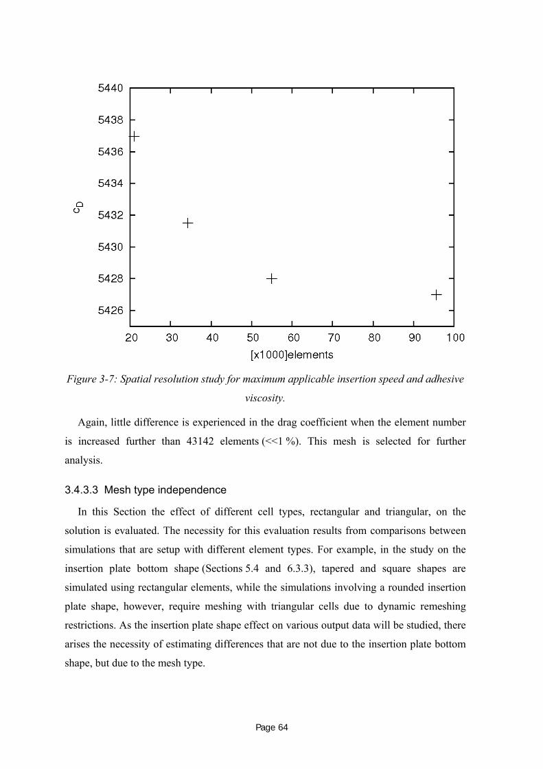
Page 64
Figure 3-7: Spatial resolution study for maximum applicable insertion speed and adhesive
viscosity.
Again, little difference is experienced in the drag coefficient when the element number
is increased further than 43142 elements (<<1 %). This mesh is selected for further
analysis.
3.4.3.3 Mesh type independence
In this Section the effect of different cell types, rectangular and triangular, on the
solution is evaluated. The necessity for this evaluation results from comparisons between
simulations that are setup with different element types. For example, in the study on the
insertion plate bottom shape (Sections 512H5.4 and 513H6.3.3), tapered and square shapes are
simulated using rectangular elements, while the simulations involving a rounded insertion
plate shape, however, require meshing with triangular cells due to dynamic remeshing
restrictions. As the insertion plate shape effect on various output data will be studied, there
arises the necessity of estimating differences that are not due to the insertion plate bottom
shape, but due to the mesh type.

Page 65
For the same problem set up in terms of design, dimensions, process and material
parameters, a comparison is conducted between the solution obtained from a simulation
that contained mainly rectangular cells and solutions for four different simulations from
meshes built up of triangular cells only. The numbers of cells for the triangular grids are
24083, 49061, 110150 and 153418. The triangular-cell based meshes were constructed in a
similar way to the construction of the rectangular-cell based meshes, i.e. the entire number
of cells was adjusted according to the number of vertical cell layers in the flow channels.
Results are compared to those from the simulation for the rectangular-cell based
mesh (43142 elements). In 514HTable 9 the drag coefficients at the insertion plate are presented
for the different solutions as well as the percent difference between the results of the
triangular and rectangular meshes.
Table 9: Mesh type independence analysis results.
Mesh type Number of elements Drag coefficient Percent difference
from rectangular
grid
triangular 24083 749 6.4
triangular 49061 729 3.7
triangular 110150 714 1.8
triangular 153418 714 1.8
mainly rectangular 43142 701 0
The drag coefficientsfor the triangular grids indicate that the predictions become
accurate to within a few percent for a mesh size of 100000 cells. Further increases in
resolution appear unwarranted given the associated increase in the computational
requirements.
Note that the difference between the triangular and the rectangular drag predictions on
the finest meshes used is 1.8 %. The reason for this difference is probably due to a
combination of factors including: errors induced due to the different remeshing schemes
for the different mesh types, under-convergence during the iterations involved in each
timestep, and small solution errors even on the finest meshes.

Page 66
It is decided to use the mesh of 110150 elements for simulations where triangular
meshes are required. The chosen meshes, both rectangular and triangular, are consistent
with prediction accuracy of a few percent.
3.4.4 Convergence
As the numerical technique applied solves for the flow variables iteratively, it is
necessary to specify a limit at which the iterative process terminates. The difference
between all numerical solutions and the solutions of the discretised equations is referred to
as a residual. The average of these residuals over all cells is specified as the global
residual, which is used as the limit to terminate further iteration. The minimal global
residuals for convergence tests are set to 10-3, 10-4 and 10-5. This means that for each
timestep iteration continues until the mass and momentum equations are satisfied to better
than these fractional accuracies. As before, the variable selected for comparison is the drag
coefficient of the insertion body. Results for the simulations are presented in 515HTable 10:
Table 10: Effect of convergence criteria on the drag coefficient at the body.
Convergence criteria Drag coefficient at body Percentage difference from
highest resolution
10-3 704.4 0.44
10-4 701.5 0.02
10-5 701.3 0
Relative to a convergence criterion of 10-4 an increase to 10-5 improved the solution
accuracy only marginally – about 0.02 %. However, the higher accuracy required results in
a significant increase in computer time. Thus, a convergence criterion of 10-4 is found to
resolve the simulation sufficiently well in a reasonable computation time and is chosen for
further simulations if not otherwise stated. Note that Fluent allows the convergence criteria
for each equation to be selected independently; however, for the simulations reported in
this thesis, the same criterion was used for all equations.
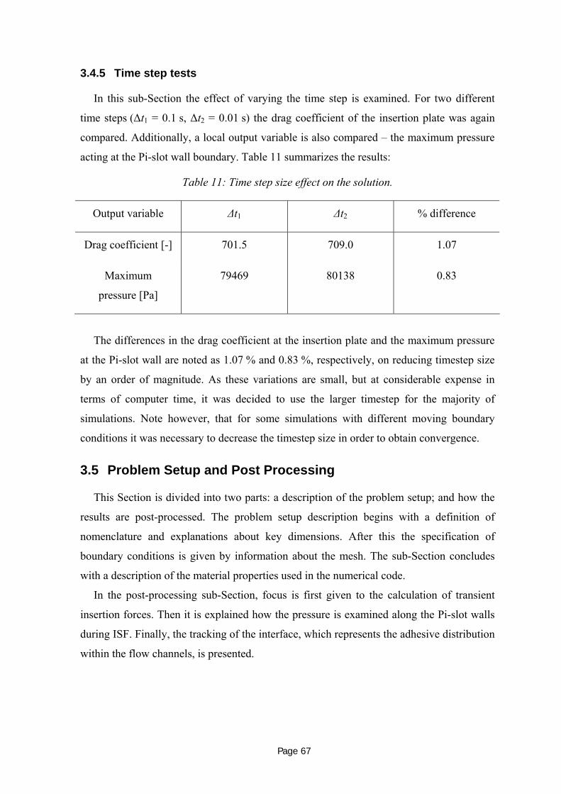
Page 67
3.4.5 Time step tests
In this sub-Section the effect of varying the time step is examined. For two different
time steps (Δt1 = 0.1 s, Δt2 = 0.01 s) the drag coefficient of the insertion plate was again
compared. Additionally, a local output variable is also compared – the maximum pressure
acting at the Pi-slot wall boundary. 516HTable 11 summarizes the results:
Table 11: Time step size effect on the solution.
Output variable Δt1 Δt2 % difference
Drag coefficient [-] 701.5 709.0 1.07
Maximum
pressure [Pa]
79469 80138 0.83
The differences in the drag coefficient at the insertion plate and the maximum pressure
at the Pi-slot wall are noted as 1.07 % and 0.83 %, respectively, on reducing timestep size
by an order of magnitude. As these variations are small, but at considerable expense in
terms of computer time, it was decided to use the larger timestep for the majority of
simulations. Note however, that for some simulations with different moving boundary
conditions it was necessary to decrease the timestep size in order to obtain convergence.
3.5 Problem Setup and Post Processing
This Section is divided into two parts: a description of the problem setup; and how the
results are post-processed. The problem setup description begins with a definition of
nomenclature and explanations about key dimensions. After this the specification of
boundary conditions is given by information about the mesh. The sub-Section concludes
with a description of the material properties used in the numerical code.
In the post-processing sub-Section, focus is first given to the calculation of transient
insertion forces. Then it is explained how the pressure is examined along the Pi-slot walls
during ISF. Finally, the tracking of the interface, which represents the adhesive distribution
within the flow channels, is presented.

Page 68
3.5.1 Problem setup
Shown on the left-hand side of 517HFigure 3-8 is a typical example of a joint considered
during the current research. This is composed of an insertion plate and a Pi-slot for the
simulation of the adhesive flow. As the joint made by the ISF process is relatively
long (typically to be more than 1000 mm in length), and the adhesive will be pre-applied
into the Pi-slot relatively uniformly along the length, it was assumed that for most cases the
adhesive flow could be simplified as a two-dimensional (2D) flow on a cross section of the
joint. Key dimensions defining the geometry to be simulated included: height of the Pi-
slot, H1, initial height of the adhesive, H0, and widths of the insertion plate and Pi-slot, 2a
and 2b, respectively. The length of the joint (dimension into the paper) is defined by w.
On the right-hand side the corresponding flow domain is illustrated. The initial adhesive
would be contained below the insertion plate before this boundary starts its downward
motion with a prescribed velocity. The rest of the domain is filled with air. The domains
above the flow channels are referred to as outflow regions. Their purpose is to provide
space to accommodate displaced adhesive and specify pressure outlets to avoid
compression.
In the flow model setup, each solid wall was specified as a wall entity, which was rigid
and impermeable with a no-slip boundary condition applied. The flow domain was then
defined between these walls and is illustrated on the right-hand side of 518HFigure 3-8.
Furthermore the insertion plate walls are specified as moving walls. A prescribed
translational motion is attached to these boundaries.

Page 69
Insertion plate
Adhesive
Pi-slot
2b
2a
H0
H1
Insertion plate width 2a
Pi-slot width 2b
Pi-slot height H1
Flow channel width δ
Outflowregions
Pressure outlets
x
y
z
c
Insertion plate
Adhesive
Pi-slot
2b
2a2a
H0
H1
Insertion plate width 2a
Pi-slot width 2b
Pi-slot height H1
Flow channel width δ
Outflowregions
Pressure outlets
x
y
x
y
zz
c
Figure 3-8: Key dimensions for 2D flow simulations (schematic and corresponding mesh).
In practice, the insertion plate can be inserted into the slot with either constant force or
constant speed. Most simulations considered a constant speed insertion. In these
simulations, the insertion plate is forced to move down at a constant speed and, in turn, the
adhesive is displaced into the side-gaps formed between the insertion plate and the Pi-slot.
Assuming a perfect alignment between the insertion plate and Pi-slot, the gap width on
each side of the insertion plate was b-a for the geometry considered. These gaps will be
referred to as flow channels in the following discussions. They become bond-lines if fully
filled by the adhesive and cured.
To enable the moving boundary, interfaces between the mesh domain that is below the
insertion plate and the mesh domain representing the flow channels have to be applied.
These interfaces are emphasized in 519HFigure 3-9.

Page 70
Moving boundary
Interfaces along vertical motion
Triangular mesh domain
Moving boundary
Interfaces along vertical motion
Triangular mesh domain
Figure 3-9: Mesh domain details indicating the moving boundaries and the necessary
interfaces between sliding elements.
The purpose of the interface is to allow a sliding between adjacent cells of different
mesh domains. In addition, in 520HFigure 3-9 the moving boundary is indicated. A triangular
mesh is used in part of the domain due to the difficulty in meshing with only quadrilateral
elements.
Except for the indicated regions and the coarse mesh domains in the outflow regions,
the rest of the domain was meshed with rectangular cells. A very similar mesh was
developed for other geometries, such as when the insertion plate bottom shape is
tapered (see 521HFigure 3-10). The insertion plate bottom shape is referred to as insertion head
shape in the following discussion. A third design uses a rounded insertion head shape. All
head shape designs are illustrated in 522HFigure 3-10. In the case of the rounded head shape
only triangular cells are used for meshing as already was indicated in the mesh type
validation study, sub-Section 523H3.4.3.3. As a consequence, a different remeshing scheme had
to be applied, which is explained in sub-Section 524H3.3.3.

Page 71
rectangular tapered roundedrectangular tapered rounded
Figure 3-10: Different insertion plate bottom shapes (also referred to as insertion head
shapes).
The fluids within the domain were modelled as two phases: air and adhesive. Material
properties that are chosen for the two phases are investigated and results are presented in
Section 525H3.4. Thus, the density of air is selected for most simulations as ρair = 1 kgm-3 and
air viscosity is specified as ηair = 0.001kgm-1s-1. In cases where convergence difficulties
were experienced these parameters had to be adjusted. The adjustment involved an
increase of air density with the limitation that the condition ρair / ρadhesive ≤ 0.01 is met. This
is in line with the free surface spinning-bowl test, discussed above, which indicated that the
predictions for the heavies phase are not sensitive to the viscosity ratio if it was at least
100. In addition, air viscosity always remains ≤ 1 kgm-1s-1. Again, previous tests indicate
that the predictions for the heavier phase are not sensitive to the viscosity ratio.
Adhesive density is specified as ρadhesive = 103 kgm-3 as given in the data sheet.
Adhesive viscosity varies according to the mixture of adhesives components. This is
modelled with the code using the power law model and the five parameter rational model.
The development of these models and the determination of coefficients characterizing each
model will be discussed in Chapter 526H4.4.5.
3.5.2 Post processing
One variable of considerable interest is the insertion force, which is equivalent to the
drag force of the insertion plate resulting from its downward motion. The insertion force
direction is the same the motion of the insertion plate. As mentioned earlier, the insertion
force is made up of two components, the pressure force at the bottom of the plate and the
viscous forces on the side walls. The insertion force can be determined from the transient

Page 72
drag coefficient along the insertion plate in the y-direction. The drag coefficient is defined
as
AUFcD 2
2ρ
= , (3-34)
with ρ being the reference density, U being the reference velocity, A being the reference
area and F being the drag force. The drag coefficient can be directly obtained from the
simulation so that the insertion force can be calculated.
The reference values can be specified and are used for post-processing only. By default,
the reference values are specified as a value of one for velocity and area and the density is
specified as air density, so that the drag coefficient and the insertion force are related as
Dc]kgms[.F 261250 −= . (3-35)
A second output variable of interest for the ISF process is the pressure distribution in
the flow domain. Pressure builds up below the insertion plate during its downward motion.
A pressure-contour plot within the flow domain as obtained from the software is illustrated
in 527HFigure 3-11:
Figure 3-11: Typical pressure-contour plot during ISF.

Page 73
The pressure distribution in the flow domain can be used to predict the quantitative
pressure that loads the composite Pi-slot walls (528HFigure 3-12). This information is vital as it
is necessary for the design of composite Pi-joints. These might distort during ISF or even
get damaged. To obtain these pieces of information from experiments would be very
complicated. The gauge pressure is plotte along the Pi-slot wall, which is indicated in
529HFigure 3-11:
Figure 3-12: Pressure distribution at the slot wall for the above presented pressure-
contour plot.
In the real case, the Pi-slot walls distort in response to the pressure resulting in an
increase in flow channel width; these events are the subject of analysis in the fluid-
structure interaction (FSI) (Section 530H7.2).
To obtain information about the distribution of both phases within the flow domain, the
VOF method is implemented. VOF prescribes flow characteristics for each cell according
to the volume fraction of each phase within each cell. In the phase transition region – that
close to the fluid-fluid interface – the volume fraction of both phases changes rapidly from
0 to 1. As this change in general occurs over a range of finite thickness, the location of the
fluid-fluid interface becomes smeared. The thickness of this interface region is largely

Page 74
determined by the spatial resolution in this region. 531HFigure 3-13 indicates the interface for a
sufficiently resolved spatial simulation:
Figure 3-13: Phases distribution within the flow domain and a detailed interface of the
flowfronts (adhesive coloure red, air in blue).
Red and blue colours represent adhesive and air, respectively. In 532HFigure 3-13 the
insertion plate has already moved into the adhesive and displaced it into the flow channels.
The remainder of the flow channels and the outflow chambers are filled with air. The
position and shape of the adhesive flow fronts are clearly indicated. For the simulations
conducted the resolution of the interface is believed to be sufficient. This view is based on
examining predictions of the interface shape and position from meshes with other
resolutions. The right-hand side of 533HFigure 3-13 illustrates a magnified view emphasizing
the shape of the adhesive flow fronts.
3.5.3 Dimensionless parameters
The adhesive flow during ISF can be characterised through two dimensionless
parameters: the Reynolds number and the Weber number.
The Reynolds number is a measure of the ratio of the inertia force on a fluid element to
the viscous force on an element (Munson, 2006). It is defined as

Page 75
ηρ lVRe = . (3-36)
In the present study, the Reynolds number is << 1, indicating viscous forces to be much
greater than inertial forces. These types of flows are referred to as Stokes flows.
The second dimensionless number, the Weber number, is important for flows with an
interface between two fluids. It relates the inertia force to the surface tension force of a
fluid element. The Weber number is defined as
σρ lVWe
2
= , (3-37)
and is less than 1 for the considered ISF. Hence surface tension forces are dominant
compared to inertial forces and are taken into consideration.
Relating the Weber number to the Reynolds number through We/Re, and hence
comparing the visous forces to the surface tension forces, we determine a value of an order
of 101 for insertion speeds of O (10-3) indicating viscous forces being dominant compared
to surface tension forces. However, reducing the insertion speed has a higher impact on the
Weber number (quadratic dependence compared to linear dependence for Re), so that
consequently surface tension forces become more important for insertions at low speeds.
3.6 Experimental Method
Over the period of the conducted research work, two sets of experimental tests on the
insertion squeeze flows were conducted with the purpose of measuring insertion forces
during insertion. These tests mainly differed in the sample sizes (short and long) and the
insertion speeds (low and high); additional information about the tests is given in the sub-
sections below.
3.6.1 Experimental equipment
Both sets of tests were conducted with the aid of an Instron universal test rig. The test
rig is a dual column system suitable for tension and compression applications. The capacity
of the machine is 10 kN, which is sufficient for insertion forces that are expected during
ISF. The tests are conducted at constant speed while recording the acting forces with
respect to time or displacement.
To eliminate effects of machine load train compliance, which might cause inaccuracies
when attempting to measure the insertion plate position using crosshead displacement, the

Page 76
displacement is measured using a linear variable differential transformer (LVDT) that is
mounted to the test sample. Machine load train compliance may be experienced through
bending of machine parts which would falsify measured displacement, which therefore is
expected to be more accurately measurable with the use of LVDTs. This inductive
displacement transducer measures the position of the insertion plate and transfers the data
to a computater. For a second set of tests – that is for the longer test samples – a second
and third LVDT were mounted on each side of the Pi-slot sample to measure the distortion
of the Pi-slot walls. The test rig, including the crosshead [1], is shown together with a
sample [2] and the mounted LVDTs [3] in 534HFigure 3-14 .
Figure 3-14: Experimental test setup to measure the insertion force versus displacement
during an ISF bonding process.
As the adhesives to be used are two component paste materials, the components have to
be mixed before inserting the adhesives into the Pi-slot and starting the ISF process.
Therefore, during the first set of experiments a dual asymmetric centrifugal mixing device
(trademark SpeedMixerTM) is used to uniformly mix the components
together (SpeedMixerTM, 2009). The rotational speed in revolutions per minute (rpm) and
the mixing time are adjustable and are chosen in a way to mix both components

Page 77
sufficiently while avoiding prolonged or intense mixing, thus avoiding viscous heating and
potential premature curing. For the second set of tests the components had to be mixed by
hand as a mixing device was not available.
3.6.2 Dimensions of specimens, process parameters and materials
As stated above the main difference between the two sets of conducted tests is the
dimension of the specimens. For the first conducted experiments, the nominal length
Linsertion plate of the square insertion plate specimen was 99.2 mm. The width 2a of the
specimen varied due to the manufacturing process between 5.02 and 5.21 mm. The
insertion plate head shape for all conducted experiments was rectangular.
The Pi-slot width 2b was 6.2±0.02 mm, the Pi-slot height H1 was 35.5 mm and the Pi-
slot length LPi-slot was 100 mm. The resulting flow channel width for a perfectly aligned
joint therefore is b-a. The Pi-slot is closed at its ends to avoid sideways adhesive outflow.
The insertion speeds for the first set of experiments were 2, 5 and 10 mm/min. The
speed was kept constant during insertion. The amount of adhesive inserted initially is about
25 volume-percent in excess of the necessary amount to fill the flow channels.
Furthermore, the viscosity is adjusted through mixing two different adhesives with each
other. These adhesives are the paste Henkel Hysol EA 9395 and the less viscous Henkel
Hysol EA 9396. The mixing ratios by weight were selected to be 70-30, 85-15 and 100-0,
EA 9395 to EA 9396. Two or three repetitions were conducted for each tested parameter
combination. A test matrix below summarizes the input parameters.

Page 78
Table 12: Test matrix for ISF experiments conducted at low insertion speed.
Test
number
2 5 10 70-30 85-15 100-0
- mm/min mm/min mm/min Weight-
percent
EA 9395 –
EA 9396
Weight-
percent
EA 9395 –
EA 9396
Weight-
percent
EA 9395 –
EA 9396
1-3 x x
4, 5 x x
6-8 x x
9, 10 x x
11, 12 x x
The composites specimens were manufactured using the vacuum assisted infusion
process (VAP). The composites comprise high tensile strength (HTS) biaxial and
unidirectional carbon fibre clutch and RTM 6 resin according to AIMS 05-04-100, IPS 05-
04-100-01, with the lay-up as described within the MoJo deliverable specification
D2.1.1 (MoJo, 2007). A detailed characterization of the two applied adhesives can be
found in Section 535H4.2.
The second set of ISF experiments was conducted at a higher constant insertion
speed (60 mm/min). This is in accordance with the required ISF process time. The
insertion plate and Pi-slot dimensions are as follows.

Page 79
Table 13: Specimen dimensions for the second row of ISF experiments.
Dimensions [mm] Insertion plate Pi-slot
2a 4.85 – 5.14 -
2b - 6.06 – 6.27
H1 200 35.5
L 279 280
Furthermore, the insertion head shape was varied, unlike for the first set of experiments.
The insertion head was not rectangular in all tests: also tested were the tapered head shown
in Figure 3-10, with tapers extending 5 mm vertically and 2 mm on each side horizontally,
and the rounded head, shown in the same figure, with 2.5 mm radii. The adhesive amount
applied initially is again 25 volume-percent in excess of the total amount necessary to fill
the flow channels. Also, the Pi-slot ends are closed in a similar fashion to the first set of
experiments.
3.7 Summary
This chapter presents a brief overview of the numerical methodology used for the
numerical experiments conducted as part of this research program. Validation studies are
performed both to test the implementation of various physical models within Fluent and
perhaps more importantly to establish that the input of the model into Fluent is set up
correctly within the software. The resolution, iterative convergence and domain size
studies establish that predictions, at least for insertion forces and pressure, have a
characteristic accuracy of a few percent or better. The chapter also provides information on
setting up the problem, assumptions made and implementation of boundary conditions.
Finally, the parameter matrices for the two sets of experiments are provided and briefly
discussed in terms of the relevance to the numerical program and the proposed ISF
applications specified as part of the Mojo program.

Page 80
4 Development of the Constitutive Adhesives Material Model
In Chapter 538H4 the development of a constitutive material model representing the
rheological properties of the adhesives used for ISF is presented. The material model will
be implemented in the computational fluid dynamics software. The materials to be
modelled are adhesives by Loctite Aerospace, Loctite Corporation, Bay Point, California,
brand names Hysol EA 9395 and Hysol EA 9396.
Within this chapter, the selection of suitable adhesive mixing ratios is presented first.
Then, in Section 539H4.2, an overview of material data provided by the manufacturer is given,
then the equipment used for the measurements is described and finally the rheological tests
to be conducted are introduced and explained. In Section 540H4.3 calibration and validation
tests are presented and discussed. In Section 541H4.4 all rheological results and the
development of the constitutive adhesive models used in the modelling are presented. The
chapter is summarised in Section 4.5.
4.1 Selection of Adhesives
As mentioned previously, two different adhesives were chosen with the purpose of
adjusting the shear viscosity. An important requirement for the choice of the mixing ratio
is that the mixture should not flow under the action to gravitation. Therefore, a test was
developed to determine the lowest mixing ratio to meet this condition. Highest viscosities
were simply determined by using only EA 9395.
A plate was placed at an angle of 60° from the horizontal and six different ratios were
mixed and applied on specified positions on the plate. Time between mixing and
application was chosen to be 120 s for each ratio. After a further 300 s the flow behaviour
was evaluated. The test set up and the final stage of all mixing ratios is shown in 542HFigure
4-1.

Page 81
Figure 4-1: Test set-up and results for suitable weight percentage ratios of EA 9395 to
EA 9396.
The mixing ratios for the samples shown are presented in 543HTable 14, numbered by
sample, with sample 1 being the leftmost one and sample 6 being the one on the far right:
Table 14: Investigated adhesive mixing ratios for determination of lowest ratio.
Amount of
adhesive
by weight-
%
Sample 1 Sample 2 Sample 3 Sample 4 Sample 5 Sample 6
EA 9395 50 60 70 80 90 100
EA 9396 50 40 30 20 10 0
From the right photograph in 544HFigure 4-1 no flow is evident for samples 4 – 6, which are
80% EA 9395, 90% EA 9395 and EA 9395. Samples 3, 2 and 1 show clear signs of flow.
However, the flow for sample 3 was quite small and so that a ratio of 70:30 weight percent
EA 9395 to EA 9396 was selected as the lowest acceptable adhesive viscosity mixture.
Ratios of 85 – 15 and 100 – 0 EA 9395 to EA 9396 mixing ratios by weight were also
investigated.
4.2 Methodology of Rheological Tests
Both the adhesives used are epoxy resins. EA 9395 contains a non-metallic filler and
therefore can be considered a suspension. EA 9396 is less viscous than EA 9395 and was

Page 82
added to adjust the viscosity. From experience little effect on the adhesive bonding
properties would be expected.
According to the material manufacturer EA 9395 is characterized as an ambient
temperature curing two-component adhesive with excellent strength properties (Loctite,
2007). Viscosities for EA 9395 were determined on a Brookfield, HBT rheometer and
ranged between 100 and 300 Pas at 25°C. Furthermore, the adhesive is characterized as
thixotropic. The two parts were mixed with each other in a 100:17 weight percent ratio of
part A to part B. The pot life is given as 95 – 100 min for a mixture of 450 g at 25°C.
EA 9396 is a low viscous two-component ambient temperature curing adhesive. Its
viscosity compared to EA 9395 is lower and the value provided by the manufacturer is
3.5 Pas measured on a Brookfield HBT rheometer at 2.1 rad/s at 25°C. The recommended
mixing ratio is 100:30 (part A: part B) by weight percent. Pot life is specified as 75 to
90 min at 25°C for a mass of 450 g.
The rheological measurements were conducted on a rotational type rheometer with the
brand name “Rheometrics Fluid Spectrometer II (RFS II)” by Rheometrics Inc., New
Jersey, USA. Several references have previously used this type rheometer and
recommended it for the measurements such as those conducted. Malkin (1994),
Sheney (1999) and Menges (2002) recommend a rotational rheometer as being suitable for
conducting rheological tests in which the shear viscosity is to be plotted versus time or
shear rate. Also, testing standards ASTM D 2196 – 05 (ASTM, 2005) and ASTM D 4440 –
01 (ASTM, 2001), which provide the recommended procedures and equipment for
rheological tests, suggest the use of a rotational or Brookfield type rheometer. As further
evidence in support of using such a rheometer it is noted that the manufacturer provided
data obtained on a Brookfield rotational rheometer.
The RFS II consists of the Control Computer, the System Control, the test station and
the test control and analysis station (Rheometrics, 1991). An oscillatory, steady or step
shearing mode is applied to the test sample and the precise response (e.g. torque) is
measured. Correlating the applied strain and resulting response the rheological properties
were determined. Principally, the RFS II contains three subsystems which are the actuator,
transducer and environmental control. All of these are directed and monitored by the
control computer which controls and directs instructions to each subsystem and receives all
information from the subsystems. The central processing unit (CPU) and the random
access memory (RAM) contain test sequences and store data, respectively. When preparing
the sample and device, linear and rotational servo control systems of the force rebalanced

Page 83
transducer (FRT) ensure that no normal force or torque is applied to the sample during
loading of the apparatus.
The set-up of the rotational discs can either contain two parallel flat plates or a cone and
plate. The advantage of the cone and plate is that the shear rate is constant across the whole
cone surface (Sheney, 1999). The cone and plate geometry was used for all testings. The
upper plate is shaped conically and mounted to the transducer. The flat circular bottom
plate is mounted to the actuator and rotates at a controlled angular velocity. A sketch of the
apparatus is shown in 545HFigure 4-2:
0.05 mmβdcone-plate
Stationary conical disc
Rotating flat disc
Testsample
Actuator
Transducer
25 mmr
θ
0.05 mmβdcone-plate
Stationary conical disc
Rotating flat disc
Testsample
Actuator
Transducer
25 mmr
θθ
Figure 4-2: Cone and plate viscometer illustration of the equipment used for the
rheological tests.
As illustrated in 546HFigure 4-2 the diameter of both discs is 25 mm and the minimum gap
between the conical and flat disc is 0.05 mm. The cone angle β of the upper plate is 0.1 rad
(5.7296°) and is determined according to the previously stated condition that a constant
shear rate should be reached on the cone surface (Sheney, 1999). The shear rate is
calculated as follows:
βθγ γγ
1== K,K && (4-1)
Within equation 547H(4-1), β is the cone angle (rad), Kγ is the strain constant (rad-1) and θ& is
the actuator angular velocity (rad/s). The dynamic strain is calculated using:
θγ γ *K= (4-2)

Page 84
To transform the measured torque T into shear stress the following relationship is
applied (Sheney, 1999):
∫ ==R
RdrrT0
2132
21 322 τππτ (4-3)
Thus, shear stress is calculated from the measured torque as:
323
RTπ
τ = (4-4)
When making the measurements, it is important that the material sample covers the
whole fixture surface without overflow. Otherwise the prior presented equations will not
obtain correct results.
The following tests were conducted:
− Shear viscosity versus time measurements for several constant shear rates, also
referred to as apparent viscosity measurements in ASTM D 2196 – 05,
− shear viscosity versus step-wise increasing shear rate measurements according to
ASTM D 2196 – 05, to derive the shear thinning characteristics of the adhesives,
also referred to as quasi-dynamic viscosity,
Time
Shear rateShear rate
ViscosityMeasurement
Time
Shear rateShear rate
ViscosityMeasurement
Figure 4-3: Method of measurements for viscosity versus stepwise increasing shear rate
tests.
− thixotropic loop test measurements of the shear viscosity with increasing and then
decreasing shear rates as described in ASTM D 2196 – 05 and Malkin (1994), to
derive the adhesives’ time-dependence,

Page 85
Time
Shear rate
Time
Shear rate
Figure 4-4: Applied shear rate with respect to time graph for the thixotropic
measurements.
− and finally viscoelastic measurements, according to ASTM D 4440 – 01, to
describe whether elastic effects have to be taken into account.
The shear viscosity versus time measurements were conducted to determine the time for
the adhesive viscosity to reach a constant value. The shear viscosity of shear thinning non-
Newtonian fluids can change at the start of measurement as described in the literature (e.g.
Menges 2002, Malkin 1994) due to the restructuring processes of macromolecules. As the
second test – the shear viscosity versus shear rate – was conducted in a step wise manner, it
is important that the shear viscosities are measured when the viscosity has reached a
constant value.
For the shear viscosity versus shear rate measurements the range of shear rates
occurring during the ISF process needs to be determined before measurements can be
conducted. Predictions for this shear rate range were determined from CFD results for a
Newtonian fluid with constant viscosity. This would not affect the acting shear rates as the
shear rate is independent of viscosity. From these simulations, the highest acting shear
rates can be expected for the highest applied insertion speeds (120 mm/min) and the
smallest flow channel widths. The shear rate range for this case was determined to be
between 0 and 200 s-1. Spatially, the highest shear rates were found to occur close to the
boundaries, hence along the Pi-slot and insertion plate walls.
Due to equipment limitations meaningful viscosity measurements can only be
conducted for shear rate ranges between 0.1 and about 30 s-1. Below 0.1 s-1 the applied test
standards cannot be applied and the transducer has insufficient sensitivity. Above 30 s-1 a
careful consideration of the sample must be conducted during testing in order to check
whether the whole cone surface area is covered. This is important because centrifugal
forces acting on the sample can cause some material under test to flow out of the testing
area, falsifying measurements.

Page 86
There are shear rates experienced during ISF that are out of the possible shear rate range
that can be tested. The developed material models cover that part of the viscosity curve in
the missing range by extrapolation of the measured values.
4.3 Calibration and Validation of Equipment
Before all measurements were taken the equipment was calibrated. This included
normal force, torque, angular velocity and alignment calibrations.
After the final measurement the equipment was again tested with a calibration liquid.
For this purpose shear viscosity was measured with respect to time and the following
results were obtained:
Figure 4-5: Shear viscosity of a calibration liquid with respect to time at a constant shear
rate of 1 s-1.
From 548HFigure 4-5 an average shear viscosity of 1.0103 Pa.S at a temperature of 22.8°C
could be determined. This shear viscosity value was compared with values provided by
Cannon ( 549HTable 15):

Page 87
Table 15: The shear viscosity of a cannon certified viscosity standard liquid silicone at
different temperatures as provided by the manufacturer.
T [°C] η [Pa.S]
20 1.123
23 1.055
25 1.033
At a temperature of 22.8°C the shear viscosity can be calculated to be 1.0595 Pa.S
applying an exponential fit between the shear viscosities at 20°C and 23°C (see 550HFigure
4-6).
Figure 4-6: Polynomial fit of the calibration liquid viscosity versus temperature.
For a temperature of 22.8°C the deviation between the manufacturer data and the
measured data was calculated as:

Page 88
04870048711010310595111 ....
measured
fitlinear =−=−=−=η
ηχ (4-5)
According to ASTM D 2196 – 05, section 7, it is reasonable to assume that a viscometer
is calibrated if the measured viscosity is within ±5% of the stated value, which is true for
the presented case. The calibration liquid viscosity was also measured for 10 1/s and
returned an average of 1.0106 Pa.S. As this is slightly higher than the shear viscosity for
100 1/s (η100 1/s = 1.0103 Pa.S) this measurement is also within the specified tolerance.
Thus, after conducting the measurements the equipment still was correctly calibrated
according to ASTM D 2196 – 05.
The procedure that was applied during the adhesive testings is described next. For each
sample preparation, the components were weighed and mixed first. The necessary mass to
fill the volume between the cone and plate was calculated to be 1.07 g. As the mixing ratio
of component A to component B of EA 9395 is 100:17 by weight it was convenient to use
1 g of component A and 0.17 g of component B. This ensured entire filling of the testing
capacity. Excessive adhesive was squeezed out and removed using a spatula as described
in ASTM D 2196 – 05 and ASTM D 4440 – 01. The procedure for mixing and weighing
when a mixture of EA 9395 and EA 9396 was used was the same except for the amount of
material applied. It was decided to mix and apply a sample of 2 g as otherwise the fractions
would get very small and therefore hard to mix and weigh. From an uncertainty analysis of
the mass applied the calculated uncertainties were 0.58 % and 0.60 % for a sample size of
2 g, hence four components, and 1 g, hence two components, respectively (Holman, 1994).
At this stage a comment is needed on the sample size proposed in ASTM D 2196 – 05:
this standard was used as it describes testing methods for rheological properties of non-
Newtonian materials. However, this testing standard applies to material samples of paint,
and therefore the sample sizes proposed are 0.5 l, i.e. very large in the current context. The
sample sizes specified in ASTM D 4440 – 01 are very small amounts of material,
approximately 3 to 5g. The ASTM D 4440 – 01 standard normally applies to materials
such as thermoplastic resins. Therefore an application of the test standard described in
ASTM D 2196 – 05 using an amount of material sample that is small and inline with the
recommendations of ASTM D 4440 – 01 seemed justified and was used in the presented
study.
As the material was mixed manually after weighing, it was decided to apply a delay
before starting the measurements. The purpose was to suppress any effects introduced into
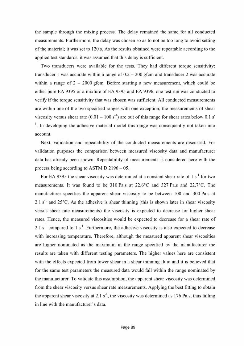
Page 89
the sample through the mixing process. The delay remained the same for all conducted
measurements. Furthermore, the delay was chosen so as to not be too long to avoid setting
of the material; it was set to 120 s. As the results obtained were repeatable according to the
applied test standards, it was assumed that this delay is sufficient.
Two transducers were available for the tests. They had different torque sensitivity:
transducer 1 was accurate within a range of 0.2 – 200 gfcm and transducer 2 was accurate
within a range of 2 – 2000 gfcm. Before starting a new measurement, which could be
either pure EA 9395 or a mixture of EA 9395 and EA 9396, one test run was conducted to
verify if the torque sensitivity that was chosen was sufficient. All conducted measurements
are within one of the two specified ranges with one exception; the measurements of shear
viscosity versus shear rate (0.01 – 100 s-1) are out of this range for shear rates below 0.1 s-
1. In developing the adhesive material model this range was consequently not taken into
account.
Next, validation and repeatability of the conducted measurements are discussed. For
validation purposes the comparison between measured viscosity data and manufacturer
data has already been shown. Repeatability of measurements is considered here with the
process being according to ASTM D 2196 – 05.
For EA 9395 the shear viscosity was determined at a constant shear rate of 1 s-1 for two
measurements. It was found to be 310 Pa.s at 22.6°C and 327 Pa.s and 22.7°C. The
manufacturer specifies the apparent shear viscosity to be between 100 and 300 Pa.s at
2.1 s-1 and 25°C. As the adhesive is shear thinning (this is shown later in shear viscosity
versus shear rate measurements) the viscosity is expected to decrease for higher shear
rates. Hence, the measured viscosities would be expected to decrease for a shear rate of
2.1 s-1 compared to 1 s-1. Furthermore, the adhesive viscosity is also expected to decrease
with increasing temperature. Therefore, although the measured apparent shear viscosities
are higher nominated as the maximum in the range specified by the manufacturer the
results are taken with different testing parameters. The higher values here are consistent
with the effects expected from lower shear in a shear thinning fluid and it is believed that
for the same test parameters the measured data would fall within the range nominated by
the manufacturer. To validate this assumption, the apparent shear viscosity was determined
from the shear viscosity versus shear rate measurements. Applying the best fitting to obtain
the apparent shear viscosity at 2.1 s-1, the viscosity was determined as 176 Pa.s, thus falling
in line with the manufacturer’s data.

Page 90
When analysing measured values against criteria for repeatability (as specified in
ASTM D 2196 – 05) it is observed that the data lies within the specified tolerance. The
tolerance specified in ASTM D 2196 – 05 is 7 % for apparent shear viscosity
measurements and 9 % for the shear thinning index. Comparing the apparent shear
viscosity data first, 551HTable 16 shows apparent viscosities determined for EA 9395 and 70 –
30 weight percent mixtures of EA 9395 to EA 9396. Deviations for each case are also
included:
Table 16: Apparent shear viscosities at different shear rates for two adhesive viscosity
ratios, indicating the deviation between two different measurements.
Weight-%
EA 9395 –
EA 9396
100 – 0 70 – 30
Shear rates
[s-1]
η1 [Pa.S] η2 [Pa.S] Deviation
(ηmax/ηmin
-1)*100
[%]
η1 [Pa.S] η2 [Pa.S] Deviation
(ηmax/ηmin -
1)*100
[%]
0.1 2350 2230 5.38 423 452 6.8
1 311 327 5.14 90 86.3 4.3
10 81.2 79.4 2.27 X X X
All presented measurements lie within the tolerances specified in ASTM D 2196 – 05
for apparent shear viscosities.
Considering shear viscosity versus shear rate measurements, ASTM D 2196 – 05
proposes comparative shear thinning indices. The shear thinning index is the ratio of the
shear viscosity at a small shear rate and the shear viscosity at a ten times larger shear rate,
e.g. shear viscosities at 0.1 and 1 s-1, 1 and 10 s-1 etc. Shear thinning indices were
determined for the conducted measurements. According to ASTM D 2196 – 05,
discrepancies are acceptable within 9%.
For EA 9395, the shear thinning indices were calculated for four shear viscosity versus
shear rate measurements. All shear thinning indices for a fraction based on shear rates of

Page 91
0.1 and 1 s-1 are within the specified tolerance, the largest deviation between two
measurements being 6.3 % (552HTable 17):
Table 17: Comparison of shear indices that were determined for EA 9395 for four different
data sets.
Shear thinning
index
Data set 1 Data set 2 Data set 3 Data set 4
η0.1/η1*100[%] 6.6 6.2 6.5 6.3
For the other considered adhesive mixtures – 70 – 30 and 85 – 15 weight percent
EA 9395 to EA 9396 – the same method was applied to judge repeatability. Both mixtures
were found to be within a deviation of 9%, the lower viscous (70 – 30) mixtures differing
by less than maximum 7.8% and the higher viscous (85 – 15) mixture showing differences
of less than 4.1%. Hence, repeatability criteria according to ASTM D 2196 – 05 were met
for all shear viscosity versus shear rate measurements.
The thixotropic loop test can be conducted according to ASTM D 2196 – 05 and the
degree of thixotropy can be determined. The degree of thixotropy is the fraction of the
shear viscosity at the lowest increasing shear rate to the shear viscosity at the lowest
decreasing shear rate. The higher determined fraction is the higher the amount of
thixotropy in the material (ASTM, 2005).
Viscoelastic measurements were conducted according to ASTM D 4440 – 01. The
storage and loss modulii were determined with respect to dynamic oscillation within the
linear viscoelastic region of the material. The linear viscoelastic region was determined
first. The relaxation time sought is defined as ( ) 12 −= fπλ , with the frequency f defined as
that when loss and storage modulus are equal (Mannan, 1995). Knowing the relaxation
time and the process time the Deborah number De can be calculated, giving an indication
whether elastic effects can be neglected or not.
4.4 Rheological Results
In this Section, shear viscosity versus time measurements are summarized before shear
viscosity versus shear rate results are presented; the adhesives’ time-dependent rheological
characteristics were determined and results of thixotropic loop tests are discussed;
measured loss and storage modulus versus strain and frequency are then presented. Results

Page 92
for both pure EA 9395 and a mixture of 70 – 30 weight-% EA 9395 to EA 9396 are
presented. Shear viscosity versus shear rate results are also presented for a mixture of 85 –
15 weight percent of EA 9395 to EA 9396. The Section concludes with a presentation of
how the material models for ISF adhesives were determined.
4.4.1 Shear viscosity versus time
EA 9395
To determine the apparent shear viscosities, the shear viscosity was measured at a
constant shear rate with respect to time. The shear viscosities were determined for three
different shear rates: 0.1, 1 and 10 s-1. Two data sets showing the apparent shear viscosity
at a constant shear rate of 0.1 s-1 are shown in 553HFigure 4-7. The first measurement (data set
1) was conducted for a period of 1200 s. The second measurement, however, was
conducted for a period of 500 s only. This was because no major changes in shear viscosity
could be detected for the first data set after about 250 s (554HFigure 4-7) and so this time period
was considered to be sufficiently long for the adhesive’s shear viscosity to reach a constant
value.
Figure 4-7: Two apparent shear viscosity graphs as a function of time for EA 9395 at a
shear rate of 0.1 s-1.

Page 93
555HFigure 4-7 demonstrates that the shear viscosity increases with time and shows how it
reaches a value of about 2320 Pa.s after 250 s for data set 1. For data set 2, at a time of
250 s the shear viscosity is 2160 Pa.s and continues to increase. This increase is relative
small compared to the entire measured data. It is 0.9 % from a measurement time of 250 s
till the end of measurement. However, the measurement time of 250 s was considered as
too long to be used in the shear viscosity versus shear rate measurements, as will be
explained in the final paragraph of this sub-Section. Therefore, a shorther measurement
time was sought, and the shear viscosities at a time of 100 s were considered more in
detail; after 100 s the shear viscosities were 2220 Pa.s and 2020 Pa.s for data set 1 and 2,
respectively, which means that the changes in apparent shear viscosities from a time of
100 s to 250 s (when the change in apparent shear viscosity is small) were 4.3 % for data
set 1 and 6.5 % for data set 2 (average of 5.4 %). Consequently, at a shear rate of 0.1 s-1 the
shear viscosity would actually be about 5.4 % higher than the one measured in shear
viscosity versus shear rate tests. Those tests are used to derive a material model for the
adhesive. The impact of the 5.4 %-discrepancy on the model derivation depends on the
accuracy of the apparent shear viscosity measurements at 100 s at shear rates higher than
0.1 s-1, which is discussed in the following paragraph.
Shear viscosities were also determined at constant shear rates of 1 and 10 s-1. The
results are presented in 556HFigure 4-8 for two data sets per shear rate:

Page 94
Figure 4-8: Two apparent shear viscosity graphs as a function of time for EA 9395, each
at shear rates of 1 s-1 and 10 s-1.
It is noticed that there is a slight overshoot in apparent shear viscosity in the first 30 s
for a shear rate of 1 s-1 and in the first 15 s for a shear rate of 10 s-1. Following this a
constant value is reached, which is an average of about 320 Pa.S and about 80 Pa.S for 1
and 10 s-1, respectively. Given these results, the material model development would hardly
be affected by the 5.4 % discrepancy experienced at 0.1 s-1.
As described previously in Section 557H4.2 the purpose of the viscosity versus time
measurements was to determine the time after which the shear viscosity reaches a constant
value. According to the results this time can be specified as 100 s. Thus, for further tests,
the shear rate was held constant for this time in the shear viscosity versus shear rate
tests (Chapter 558H4.4.2). After 100 s it was increased to the next shear rate and the same
process applied. Five measurements were taken per decade.
If the time period was taken as 250 s, based on 559HFigure 4-7, the measurements for one
decade would have taken 1250 s. Three shear rate decades had to be measured (0.1 to
100 1/s) which means a testing time of 3750 s. This time would have resulted in curing
effects becoming evident during measurements, which clearly was undesirable. Therefore,
as changes in shear viscosity of about 5% were determined to occur after 100 s (discussion

Page 95
560HFigure 4-7), this time period was applied for the shear viscosity versus shear rate
measurements. The total measurement time was then 1500 s which is a reasonable
compromise in providing accurate results without material setting effects.
EA 9395 and EA 9396 mixture (70 – 30)
The same procedure as described for the 100% EA 9395 was applied for the 70 – 30
weight percentage mixture of EA 9395 to EA 9396. The tested shear rates were 0.1 and 1 s-
1. No tests were conducted for 10 s-1 because it is assumed that similar trends would be
observed to those seen for 100% EA 9395; this is that a constant apparent shear viscosity is
reached earlier for higher shear rates. This trend is also observed for the 70 – 30
measurements, as illustrated in 561HFigure 4-9, where the shear viscosity is plotted with respect
to time for 0.1 and 1 s-1:
Figure 4-9: Two apparent shear viscosity graphs as a function of time for a 70 – 30 weight
percentage mixture between EA 9395 and EA 9396, each at shear rates of 0.1 s-1 and 1 s-1.
562HFigure 4-9 shows that for 0.1 s-1 the shear viscosity increases continuously for a time of
500 s. However, major changes occur only at the start of the measurement. From 100 to
500 s the shear viscosity of data set 1 changes 8.9 % and that of data set 2 12 %. As the

Page 96
changes from 100 s onwards are relative small, a period of 100 s was selected as the
constant shear rate time for the shear viscosity versus shear rate measurements.
Apparent viscosity measurements at a constant shear rate of 1 s-1 do not show any major
changes after the initial peak. Data set 2 remains constant; data set 1 shows a 3.5 %
increase with time so it was considered justified neglecting it. As discussed previously for
the EA 9395 adhesives only, for shear viscosity versus shear rate measurements a testing
period per constant shear rate of 100 s appeared to be a good compromise to ensure
meaningful results in a reasonable testing time.
4.4.2 Shear viscosity versus shear rate
EA 9395
Four measurements of the shear viscosity versus stepwise increasing shear rate are
presented in 563HFigure 4-10. The shear rates range from 0.01 to 100 s-1 but due to difficulties
experienced during testing only one measurement (data set 2) was conducted over the full
range. The other measurements had to be terminated after 39.8 s-1(data set 3 and 4) and
25.1 s-1(data set 1).
Figure 4-10: Four data sets showing shear viscosity as a function of shear rate
measurements for 100% EA 9395.

Page 97
All graphs are very similar in shape indicating a non-Newtonian, shear thinning material
behaviour. An initially minor increase is followed by a continuous decrease of the
logarithmic shear viscosity with logarithmic shear rate. In Section 564H4.3 we mentioned that
data below 0.1 s-1 is less accurate due to insufficient transducer resolution for the very
small shear rates. Hence, the region between 0.01 and 0.1 s-1 was not be considered when
deriving the adhesive material model.
However, this initial increase was still considered with a view to explaining it.
Measurements of shear viscosity versus constant shear rate for shear rates of 0.01 s-1,
which are not presented here, showed that after a period of 100 s the apparent shear
viscosity still increased quite significantly, most probably as restructuring processes of
macromolecules within the sample still occur. Hence, considering the results presented
here we believe that for the second constant shear rate of 0.0251 s-1 the unfinished
restructuring processes of macromolecules lead to an increased shear viscosity.
The differences experienced between the different data sets are most probably due to
differences in temperature during testing which varied between 20.4 and 21.7°C. For data
set 1 the testing temperature was the lowest compared to the other data sets. The derivation
of the material model was based on the average data from these measurements for a shear
rate range between 0.1 and 25.1 s-1.
Inconsistencies between data sets where data is available occur for shear rates higher
than 25.1 s-1 e.g. data set 2 shows a sudden drop in shear viscosity between 25.1 and 39.8 s-
1. At this shear rate detachments of the sample and the cone surface were observed.
Equations 565H(4-3) and 566H(4-4) used to calculate torque and shear stress, respectively, are
restated to explain the effect detachment has on the determination of the shear viscosity:
∫ ==R
RdrrT0
2132
21 322 τππτ (4−3)
323
RTπ
τ = (4−4 )
The integration limit R in equation 567H(4-3) is smaller for the cases where the cone surface
was not covered completely with the sample. If R was smaller the shear stress value would
become larger (equation 568H(4-4)). If the shear stress was larger the shear viscosity would
become larger as the shear viscosity is the ratio of shear stress and shear
rate (equation 569H(4-6)):

Page 98
γτη&
= (4-6)
Thus, shear viscosity of data set 2 should be larger than presented at a shear rate where
detachment occurs, in this case 38.9 s-1.
Finally, we compare the averaged values of these measurements with results that were
obtained from apparent shear viscosity measurements.
Table 18: Effect of the test type – either apparent or quasi-dynamic viscosity - on shear
viscosity data at three different shear rates.
Shear rate Apparent shear viscosity Quasi dynamic shear viscosity
[1/s] [Pa.s] [Pa.s]
0.1 2120 1822.5
1 319 283.5
10 80 82.5
Discrepancies between data from both test types are evident and reasons for these
discrepancies are not obvious. One possible explanation is that the adhesive is time
dependent with the viscosity changing with time. To evaluate this explanation, thixotropic
loop tests were conducted and results are presented sub-Section 570H4.4.3.
Another explanation is the possibility of micro-curing occuring in the adhesive, causing
an increase in shear viscosity. Occurrence of micro-curing can be caused by the shearing of
the adhesives as this is larger for the shear viscosity versus shear rate measurements than
for the apparent viscosity measurements. Considering the viscosity change with increasing
shear rate, we notice that the rate of change is greater for the apparent shear viscosity
measurements. For example the apparent viscosities are greater for 0.1 and 1 s-1, but
smaller for 10 s-1, so the longer the quasi dynamic test lasts the greater its viscosity value
as more shear was induced on the sample.
It also is possible that the temperature variation, from 20.4 to 21.7°C, affects the shear
viscosities. However, this seems doubtful as no particular trend can be observed. The
apparent shear viscosity measurements were taken at higher as well as lower temperatures
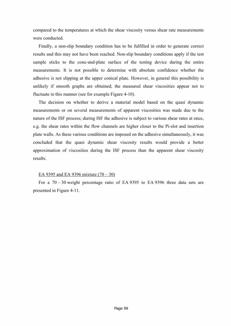
Page 99
compared to the temperatures at which the shear viscosity versus shear rate measurements
were conducted.
Finally, a non-slip boundary condition has to be fulfilled in order to generate correct
results and this may not have been reached. Non-slip boundary conditions apply if the test
sample sticks to the cone-and-plate surface of the testing device during the entire
measurements. It is not possible to determine with absolute confidence whether the
adhesive is not slipping at the upper conical plate. However, in general this possibility is
unlikely if smooth graphs are obtained; the measured shear viscosities appear not to
fluctuate in this manner (see for example 571HFigure 4-10).
The decision on whether to derive a material model based on the quasi dynamic
measurements or on several measurements of apparent viscosities was made due to the
nature of the ISF process; during ISF the adhesive is subject to various shear rates at once,
e.g. the shear rates within the flow channels are higher closer to the Pi-slot and insertion
plate walls. As these various conditions are imposed on the adhesive simultaneously, it was
concluded that the quasi dynamic shear viscosity results would provide a better
approximation of viscosities during the ISF process than the apparent shear viscosity
results.
EA 9395 and EA 9396 mixture (70 – 30)
For a 70 – 30 weight percentage ratio of EA 9395 to EA 9396 three data sets are
presented in 572HFigure 4-11.

Page 100
Figure 4-11: Three data sets showing shear viscosity as a function of shear rate
measurements for 70 – 30 weigth percentage mixtures of EA 9395 to EA 9396.
A similar graph shape as the one for EA 9395 is observed, indicating a shear thinning
material characteristic. In general, shear viscosities are lower compared to EA 9395. This
is expected as the lower viscous adhesive EA 9396 is added to the sample.
The shear viscosities at higher shear rates, i.e. above 25.1 s-1, seem to continue its
smooth decreasing shape. A judgement about detachment is hard to conduct but it appeared
that for these mixtures the cone surface remained covered with adhesive during the entire
testing period.
A comparison between apparent shear viscosity measurement data and quasi dynamic
shear viscosity data is presented in 573HTable 19.

Page 101
Table 19: Adhesive shear viscosities determined from apparent and quasi dynamic tests at
different shear rates for 70 – 30 weight percentage mixtures of EA 9395 to EA 9396.
Shear rate Apparent shear viscosity Quasi dynamic shear viscosity
[s-1] [Pa.s] [Pa.s]
0.1 423 452 424 401 346
1 90 86 83 83 74
Little differences are noticeable for shear viscosities for different test types. The
apparent shear viscosity values are slightly higher with one exception which is data set 1
for 0.1 s-1.
EA 9395 and EA 9396 mixture (85 – 15)
Lastly, shear viscosity versus stepwise increasing shear rates is presented for a mixing
ratio of 85 – 15 weight percent EA 9395 to EA 9396. The data are illustrated in 574HFigure
4-12.

Page 102
Figure 4-12: Shear viscosity as a function of shear rate measurements from two data sets
for a 85 – 15 weigth percentage mixture of EA 9395 to EA 9396.
A shear thinning non-Newtonian behaviour is observed as in the two previously
presented measurements within Chapter 575H4.4.2. A comparison with data for the 70 – 30
mixture is conducted and presented in 576HTable 20. In the table it is noticed that the shear
viscosity differences between 85 – 15 and 70 – 30 are larger for smaller shear rates. For
0.1 1/s the shear viscosity of 85 – 15 is almost double that for 70 – 30. For a shear rate of
100 1/s the shear rates are almost identical. This trend – that the shear viscosity differences
decrease with increasing shear rate – could be explained as follows: It is shown that
EA 9395 is clearly a non-Newtonian shear thinning fluid. The material manufacturer
provides a constant shear viscosity of 3.5 Pa.S for EA 9396, indicating that the adhesive
shear viscosity is independent of shear rate, and therefore a Newtonian fluid. If it is
assumed that EA 9395 is shear thinning and the addition of 15 weight percent EA 9396
decreases the shear viscosity, a combination between shear thinning and decreased shear
viscosity might lead to the observed results. For a 70 – 30 weight percent ratio the shear
thinning effect is smaller and therefore might lead to similar shear viscosities compared to
a 85 – 15 weight percent ratio mixture for higher shear rates.

Page 103
Table 20: Adhesive shear viscosities determined from apparent and quasi dynamic tests at
different shear rates for 85 – 15 and 70 – 30 weight percent mixtures of EA 9395 to
EA 9396.
Quasi dynamic shear viscosity
Shear rate 85 – 15 70 – 30
[s-1] [Pa.s] [Pa.s]
0.1 809 672 424 346
1 130 113 83 74
10 39 37 32 30
100 24 24 24 23
4.4.3 Time-dependence
During the thixotropic loop tests the shear rate was increased from 0.1 s-1 to 30 s-1 and
to 10 s-1 while recording the shear stress and then decreased through the same range. The
loop duration was 300 s in total, i.e. the shear rate was increased within the first 150 s and
then decreased within the next 150 s. This duration was varied in another measurement
where the entire loop was conducted within 20 s only. Two measurements were conducted
for each loop and the typical shear stress versus shear rate graphs are presented in 577HFigure
4-13 and 578HFigure 4-14 for EA 9395.

Page 104
Figure 4-13: Shear stress versus shear rate for a thixotropic loop test for 100% EA 9395
(300 s loop).
Figure 4-14: Shear stress versus shear rate for a thixotropic loop test for 100% EA 9395
(20 s loop).

Page 105
It is observed that the shear stress increases with increasing shear rate and then
decreases with decreasing shear rate. The degree of thixotropy is defined in ASTM D 2196
– 05 as the ratio between shear viscosity at the lowest shear rate for increasing shear rates
and shear viscosity at the lowest shear rate for decreasing shear rates. In the above
presented figures the degree of thixotropy is 1.20 and 1.04 for the 300 s loop and the 20 s
loop, respectively. According to Uhlherr (2009), these loops show little thixotropy.
The differences in the shear stress for the lowest shear rates for the increasing and the
decreasing shear rate range presented for the 300 s loop shown in 579HFigure 4-13 most
probably resulted again from difficulties experienced during the measurements at higher
shear rates (Uhlherr, 2009). At those shear rates outflow of the test sample due to
centrifugal forces can occur. To avoid the possible outflow and hence effect on the results,
the thixotropic loop for 300 s measurement time was repeated for a shear rate range from
0.1 to 10 s-1. Results are shown in 580HFigure 4-15.
Figure 4-15: Thixotropic 300 s loop for a shear rate range from 0.1 to 10 s-1 for 100 %
EA 9395.
The graphs obtained for both shear stress branches show little difference for the lowest
tested shear rates compared to the results presented in 581HFigure 4-13. The degree of
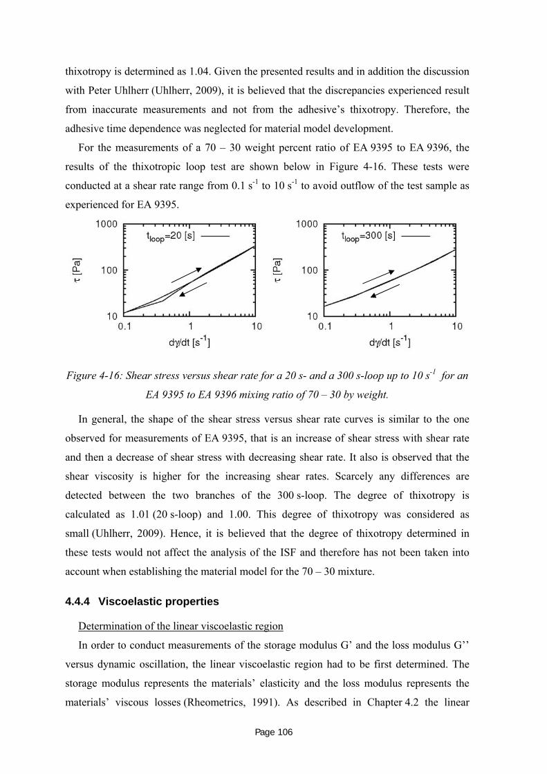
Page 106
thixotropy is determined as 1.04. Given the presented results and in addition the discussion
with Peter Uhlherr (Uhlherr, 2009), it is believed that the discrepancies experienced result
from inaccurate measurements and not from the adhesive’s thixotropy. Therefore, the
adhesive time dependence was neglected for material model development.
For the measurements of a 70 – 30 weight percent ratio of EA 9395 to EA 9396, the
results of the thixotropic loop test are shown below in 582HFigure 4-16. These tests were
conducted at a shear rate range from 0.1 s-1 to 10 s-1 to avoid outflow of the test sample as
experienced for EA 9395.
Figure 4-16: Shear stress versus shear rate for a 20 s- and a 300 s-loop up to 10 s-1 for an
EA 9395 to EA 9396 mixing ratio of 70 – 30 by weight.
In general, the shape of the shear stress versus shear rate curves is similar to the one
observed for measurements of EA 9395, that is an increase of shear stress with shear rate
and then a decrease of shear stress with decreasing shear rate. It also is observed that the
shear viscosity is higher for the increasing shear rates. Scarcely any differences are
detected between the two branches of the 300 s-loop. The degree of thixotropy is
calculated as 1.01 (20 s-loop) and 1.00. This degree of thixotropy was considered as
small (Uhlherr, 2009). Hence, it is believed that the degree of thixotropy determined in
these tests would not affect the analysis of the ISF and therefore has not been taken into
account when establishing the material model for the 70 – 30 mixture.
4.4.4 Viscoelastic properties
Determination of the linear viscoelastic region
In order to conduct measurements of the storage modulus G’ and the loss modulus G’’
versus dynamic oscillation, the linear viscoelastic region had to be first determined. The
storage modulus represents the materials’ elasticity and the loss modulus represents the
materials’ viscous losses (Rheometrics, 1991). As described in Chapter 583H4.2 the linear

Page 107
viscoelastic region can be evaluated through measurements of the storage and loss moduli
with respect to strain for a constant frequency. Results presented in 584HFigure 4-17 and 585HFigure
4-18 illustrate shear and loss moduli measurements for increasing strains at a constant
frequency of 100 rad/s for EA 9395 and the 70 – 30 weight percent ratio mixtures of
EA 9395 to EA 9396.
Figure 4-17: Storage and loss modulus versus strain at a frequency of 100 rad/s (100 – 0).
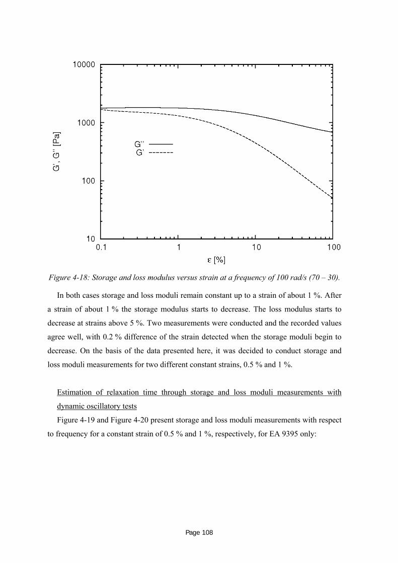
Page 108
Figure 4-18: Storage and loss modulus versus strain at a frequency of 100 rad/s (70 – 30).
In both cases storage and loss moduli remain constant up to a strain of about 1 %. After
a strain of about 1 % the storage modulus starts to decrease. The loss modulus starts to
decrease at strains above 5 %. Two measurements were conducted and the recorded values
agree well, with 0.2 % difference of the strain detected when the storage moduli begin to
decrease. On the basis of the data presented here, it was decided to conduct storage and
loss moduli measurements for two different constant strains, 0.5 % and 1 %.
Estimation of relaxation time through storage and loss moduli measurements with
dynamic oscillatory tests
586HFigure 4-19 and 587HFigure 4-20 present storage and loss moduli measurements with respect
to frequency for a constant strain of 0.5 % and 1 %, respectively, for EA 9395 only:

Page 109
Figure 4-19: Storage and loss modulus versus frequency for a constant strain of 0.5 % for
100 % EA 9395.
Figure 4-20: Storage and loss modulus versus frequency for a constant strain of 1 % for
100 % EA 9395.
λ0.5% = 1/(2πf)

Page 110
Both moduli increase with increasing frequency, and the loss modulus in both cases
shows a steeper slope. The frequency at which the two graphs intersect is 55 rad/s for
0.5 % and 45 rad/s for 1 % strain. The reciprocal multiplied by 2π determines the
relaxation time which results in λ0.5% = 2.865 10-3 s and λ1% = 3.501 10-3 s.
For a 70 – 30 weight percent mixing ratio the measurements were only conducted at a
strain of 1 % as a longer relaxation time was known to occur for EA 9395 in this case.
Results are shown in 588HFigure 4-21:
Figure 4-21: Storage and loss modulus versus frequency for a constant strain of 1 % (70-
30).
As for EA 9395 the storage and loss moduli increase with frequency at different rates,
the loss modulus increases at a higher rate. The graphs intersect at a frequency of 30 rad/s,
resulting in a relaxation time of λ70-30, 1% = 5.305 10-3 s.
All relaxation times presented here are in the order of 10-3 s. Estimated process times
for ISF are about 60 s. To calculate the Deborah number De the relaxation time is divided
by process time (Menges, 2002).

Page 111
processtDe λ
= (4-7)
Taking the longest relaxation time determined, which is for 70 – 30 weight percent
EA 9395 to EA 9396 (λ70-30, 1% = 3.979 10-3 s), the De was calculated to 6.63 10-5. As
De << 1, elastic effects are assumed to be negligible for the adhesives used in ISF.
4.4.5 Constitutive model development
The adhesive material model development for EA 9395 was based on the average of
four different shear viscosity versus shear rate measurements that were presented in sub-
section 589H4.4.2. A shear viscosity plot with respect to stepwise increasing shear rate was
illustrated in 590HFigure 4-10 on page 96.
According to ASTM D 2196 – 05 the testing should only be applied for shear rates
higher than 0.1 s-1 and, as mentioned previously, our transducer resolution was insufficient
for measuring shear viscosities below 0.1 s-1. Hence, shear viscosities below 0.1 s-1 have
not been included in the adhesive model development. Furthermore, measurements taken
above a shear rate of 25.1 s-1 were also not considered due to the sample detachment
problems, also previously explained. For the 85 – 15 and 70 – 30 mixtures the average was
taken out of two and three measurements for the same shear rate ranges.
In 591HFigure 4-22, material models derived for EA 9395 and mixtures of EA 9395 to
EA 9396 are shown based on results presented in sub-section 592H4.4.2:

Page 112
Figure 4-22: Power law viscosity fits for EA 9395 and mixtures of EA 9395 and EA 9396.
In all cases the shear viscosities were fit with a power law relationship to shear rate. The
power law models appear to provide only an approximate fit to the measure of shear
viscosities. It is clear that they do not account for all variation, given the residual curvature
when plotted in log-log form. This necessitates a refined fit, which is outlined and
discussed below.
When applying the power law model, the specification of minimum and maximum
viscosity limits for very high and very low shear rates was required. If this were not done
at these extreme shear rates the viscosity would tend towards infinity for very low shear
rates and zero for very high shear rates; this would clearly be contradictory to the adhesive
behaviour in those shear rate regions.
Hence, a second fit was proposed. For all adhesives, a five parameter rational fit was
applied and is plotted in combination with experimental data in 593HFigure 4-23:

Page 113
Figure 4-23: Five parameter rational model fit for all adhesives mixtures.
The new fit matches the recorded measurements better than the power law model,
especially for higher shear rates, and also agrees well for low shear rates. Furthermore, no
viscosity limits have to be applied for very low or high shear rates as would be necessary
for the power law models. The equation for the five parameter rational model fitting is:
2
2
1 γγγγη&&
&&
edcba
++++
= . (4-8)
The parameters for EA 9395, 85 – 15 and 70 – 30 weight percent ratios of EA 9395 to
EA 9396 can be found in 594HTable 21:

Page 114
Table 21: Parameters for the five parameter rational model fit that are used to define the
adhesive mixtures viscosities.
Weight
percentage
EA 9395 –
EA 9396
a b c d e
100-0 16024.99 13515.67 1080.79 83.276 23.120
85-15 5293.645 6541.795 891.0529 66.909 36.160
70-30 1738.666 2216.062 318.678 38.981 13.796
4.5 Summary
Appropriate mixing ratios between the adhesives EA 9395 and EA 9396 according to
ISF bonding process requirements were determined as 70 – 30 weight percent of EA 9395
to EA 9396 for the lowest and 100 % EA 9395 for the highest possible adhesive viscosity.
The methodology of rheological testings was presented along with calibration of the
equipment and description and validation of the tests to be conducted. The adhesives tested
showed small time-dependence and small viscoelasticity. Two material models were
determined to specifiy the adhesive shear viscosity with respect to shear rate best, the
power-law and the five parameter rational model.

Page 115
5 Insertion Squeeze Flow at Constant Insertion Speed
5.1 Analytical and Numerical Solutions for Insertion Squeeze Flow with Newtonian Fluids
An analytic solution was derived for the flow of a Newtonian fluid during ISF
conducted at constant insertion speed. We adopted a method that was applied for a similar
flow problem and modified it where necessary. This method was applied by Smith, Ferry
and Schremp (Smith et al., 1948) to investigate the force required when a rod penetrates
into a Newtonian fluid contained in a cylinder; the fluid, in turn, is forced to rise between
the walls of the cylindrical vessel and the rod. While the problem that they analysed is axi-
symmetric, we assumed in-plane two-dimensional (2D) flow in our problem. A perfect
alignment between the insertion plate and Pi-slot was also assumed such that only half of
the domain needed to be considered.
The set up of our problem is illustrated in Figure 5-1. In the figure, h is the displacement
of the insertion plate, V is the constant insertion speed, c is the adhesive flow front in the
flow channel referenced to the initial adhesive height H0, and v(x) is the adhesive flow
velocity in negative y-direction (insertion direction) and was assumed to be a function of x
only.
Width into page: w
V, F
NewtonianFluid, η
t = t0 t > t0
2a
2b
c,v(x)
hH0
x
y
Width into page: w
V, F
NewtonianFluid, η
t = t0 t > t0
2a
2b
c,v(x)
hH0
Width into page: w
V, F
NewtonianFluid, η
t = t0 t > t0
2a
2b
c,v(x)
hH0
x
y
x
y
Figure 5-1: Key dimensions for the analysis of insertion squeeze flow with a Newtonian
fluid.

Page 116
The relationship between c and h was derived by applying the principle of mass
conservation, from which the flow front c can be determined, as follows:
aba)hH(c−
−=0
(5-1)
Balancing pressure and viscous forces on an infinitesimally small Newtonian fluid
element in the flow channel led to (Schroeder, 2000)
02
2
=∂∂
+∂∂
−xv
yp η (5-2)
where p is pressure and η is the viscosity. Note that the derivation presented was based
on two assumptions to simplify the model: the pressure p and velocity v are functions of y
and x, respectively, only.
2dx
x∂∂
+ττ
2dx
x∂∂
−ττ
2dy
ypp
∂∂
−
2dy
ypp
∂∂
+
2dx
x∂∂
+ττ
2dx
x∂∂
−ττ
2dy
ypp
∂∂
−
2dy
ypp
∂∂
+
Figure 5-2: Force balance between pressure and shear stress on an infinitesimally small
Newtonian fluid element (Schroeder, 2000).
Double integration of the force balance equation 595H(5-2) with regard to x and solving for
the integration constants with no-slip boundary conditions at x = a and at x = b, the
following expression for the velocity distribution with respect to x was obtained:
21
21
21 2 ab
yp
ηbabVxba
yp
ηbaVx
yp
ηv(x)
∂∂
+−
+⎟⎟⎠
⎞⎜⎜⎝
⎛ +∂∂
−−
−+∂∂
= (5-3)
To determine the pressure gradient the principle of mass conservation was used again.
The mass flow rates into and out of the control volume have to be equal. The following
expression was obtained:

Page 117
36)ba(
abVyp
−
+=
∂∂ η (5-4)
Assuming a linear pressure increase in the negative y-direction, the pressure gradient
with respect to y can be written as
cP
yp
−=∂∂ , (5-5)
where P is the pressure acting on the insertion plate.
Combining Equations 596H(5-5) and 597H(5-6), the pressure P was obtained as
36)ba(
abcVP−+
−= η . (5-6)
Finally, the total insertion force was considered to be made up of two
components (Smith et al., 1948): a pressure force due to pressure built up at the bottom of
the moving insertion plate and a viscous drag force at the contact surface between the
insertion plate and the Newtonian fluid. This can be expressed as
PAxvAPAAF
aywall 2121 +
∂∂=+=
=ητ , (5-7)
where F is the insertion force, τwall is the viscous drag shear stress, and A1 and A2 are the
areas on which the viscous drag shear stress and pressure act, respectively.
Substituting each of the above-derived expressions into Equation 598H(5-7), the insertion
force required for a Newtonian fluid was determined per length-unit as
⎥⎥⎦
⎤
⎢⎢⎣
⎡
−+
−
++−=
ba)ba(
)ab)(ba(cVwF 132
3η . (5-8)
The above equation indicates that for a Newtonian fluid, the insertion force increases
linearly with viscosity, insertion speed and flow front.
Insertion forces calculated applying equation 599H(5-8) were compared with numerical
predictions of the insertion forces and results are presented in 600HFigure 5-3 and in 601HFigure 5-4.
Dimensions, insertion speed and Newtonian fluid viscosity were identical for both models.
In 602HFigure 5-3 the input parameter that was varied is the insertion speed.

Page 118
Figure 5-3: Numerically and analytically predicted insertion forces as a function of
dimensionless time for different insertion speeds for an ISF process with a Newtonian
fluid.
The insertion force increases linearly with respect to time over the time range
considered. Further, the insertion force also increases linearly with respect to insertion
speed. For example, increasing the insertion force by a factor of two (5 to 10 mm/min)
leads to an approximately doubling of the insertion force (at t* = 1, the numerical
predictions were 4842 N/m to 9782 N/m).
The numerically predicted and analytically calculated insertion forces exhibited small
differences. At 2 mm/min the differences are 5.6 %, at 5 mm/min they are 4.0 % and at
10 mm/min 4.7 %. The numerical model consistently predicts higher insertion forces.
The differences observed between the analytical and numerical insertion force
predictions are caused by simplifications in the analytical model. The factors include the
neglect of hydrostatic pressure and the air phase, and the simplification to just one-
dimensional flow. In addition, as discussed previously, the second phase (air) density for
the numerical model is increased by an order of magnitude to improve the stability of the
computations. Of these factors, the neglect of hydrostatic pressure and the different

Page 119
treatment of the second phase should account for a difference of less than a percent
between the models. The main difference is presumably caused by the simplification to
one-dimensional flow in the analytic model. At the base of the insert the flow must be two-
dimensional as the fluid passes from the bottom region into the gaps.
The effect of a variation of the fluid viscosity on the insertion force was also compared:
Figure 5-4: Numerically and analytically predicted insertion forces as a function of
dimensionless time for different fluid viscosities for an ISF process with a Newtonian fluid.
Similar to the above-presented effect of the insertion speed on the insertion force, it is
found that the insertion force varies linearly with the viscosity. The insertion force also
increases linearly with time. The numerical model again predicts higher insertion forces
than the analytical model. The discrepancies are 3.60 %, 3.96 % and 3.78 % for 2000, 1000
and 500 Pa.s, respectively. The causes of these differences are the same as those discussed
above for the effect of insertion speed.
Finally, the flow velocity distribution v(x) within the flow channel was compared using
one specific case of vins = 5 mm/min and ηfluid = 1000 Pa.s. The results are illustrated in
603HFigure 5-5.

Page 120
Figure 5-5: Comparison of the velocity distribution with respect to flow channel position
predicted from the analytical and numerical models.
An x-position of 0 and 0.5 mm represents the right insertion plate side wall and the right
Pi-slot wall, respectively. The fluid velocity is negative and equal in magnitude to the
insertion speed of the insertion plate at x = 0 mm. At the other boundary the fluid velocity
is 0. Both observations can be explained through the conditions set at the wall boundaries,
where the no-slip condition was applied, resulting in the fluid velocity being equal to the
velocity of the boundaries.
The integrated area under the two graphs is identical. This area is the volume flow per
unit length and represents the amount of displaced fluid. Given the areas are equal it can be
deduced that the continuity condition is fulfilled.
There is a small discrepancy in the shape of the velocity distributions, with the
analytical solution showing a slightly higher maximum. This is attributable to the
assumptions made when solving the problem analytically. The flow velocity v in the flow
channel was assumed to vary only with x, and the pressure in the flow channel in the
insertion direction was assumed to vary only with y. As equation 604H(5-3) shows, the flow
velocity is considered a function of the pressure distribution in the insertion direction so

Page 121
the pressure constraints will also affect the fluid velocity. These simplifications were not
imposed on the numerical model, hence it is expected that they account for some small
discrepancies in the solutions, which are expressed through the observed small differences
in the velocity profiles.
In summary, an analytical solution for the considered squeeze flow problem for purely
Newtonian fluids in the specified geometry has been presented. A comparison was
conducted between analytical and numerical predictions for the insertion force and the
maximum difference was found to be 5.6 %. The difference results from differing
assumptions for the numerical and the analytical model. In both models the insertion force
has been found to linearly depend on the insertion speed and also to linearly depend on the
fluid viscosity. Another comparison was drawn between the flow velocity distributions
within the flow channels and it has been found that the flow velocities are identical for
both models at the wall boundaries and, further, that continuity is maintained in both cases.
5.2 Insertion Squeeze Flow at Low Insertion Speeds
The main objective of this section was to draw a comparison between numerically
predicted and experimentally measured insertion forces acting during ISF at low constant
insertion speeds. First, the effects of insertion speed and adhesive viscosity on the insertion
force were examined by analysing predictions obtained from the CFD simulation. Then,
results from insertion force measurements during ISF experiments conducted on a
universal Instron testing rig are presented. Finally, a comparison is made between the
numerical and experimental insertion forces.
As described in Section 605H3.5 the ISF process was modelled two-dimensionally (2D) on a
cross section of the joint (consider 606HFigure 3-8 on page 607H69). A constant speed condition was
applied on the wall boundaries that represent the insertion plate walls. Due to this motion
the adhesive was displaced into the flow channels that form between the insertion plate
side wall and the Pi-slot wall boundaries. The input parameters that were varied were the
insertion speed and the adhesive viscosity. The insertion speeds investigated were 2.5, 5
and 10 mm/min.
The adhesive viscosity was adjusted according to suitable weight percent ratios of the
higher viscous EA 9395 and the lower viscous EA 9396. The selected ratios were 70 – 30,
85 – 15 and 100 – 0 weight percent EA 9395 to EA 9396 which were derived in
Section 608H4.1. The material model to represent the adhesive viscosity was the power law
model although the five parameter rational model provided a much closer approximation of

Page 122
the measured viscosities (compare 609HFigure 4-22 and 4─23). The power law model offers an
easily implemented and low computational cost viscosity model that results in small errors
at the low strain rates that would be found at low insertion speeds. However, it is clear that
for a broader range of insertion speeds a better model is needed and this is discussed
below.
Shear rate distributions within one flow channel for the highest and the lowest applied
insertion speeds are shown in 610HFigure 5-6.
Figure 5-6: Numerically predicted shear rates in the adhesive within the flow channel for
insertion speeds of 2 and 10 mm/min.
The x-axis represents the position along a horizontal line within the flow channel that is
fully occupied by adhesive. The 0 mm x-position is at the wall boundary of the insertion
plate while an x-position of 0.5 mm represents the Pi-slot wall boundary. The shear rate
maxima are found at the insertion plate wall boundary and are 19 s-1 and 5.2 s-1 for the
higher and the lower insertion speed, respectively. With increasing distance from this
boundary the shear rate decreases and reaches a minimum at an x-position of 0.255 mm.
As the shear rate is defined as a function of the second invariant of the rate-of-deformation
tensor (see equations 611H(3-17) and 612H(3-19) on page 613H50) and the y-component of the velocity

Page 123
vector reaches its maximum at an x-position of 0.255 mm (see 614HFigure 5-5), the shear rate at
this position is expected to be 0 given the rate of change of the x-component of the velocity
vector is negligible. This indeed is predicted in the numerical model but not illustrated in
615HFigure 5-6 due to insufficient resolution in the region around 0.25 mm. In fact the shear
rate, which is effectively |∂v/∂x|, will have a discontinuous gradient as it reaches zero. The
shear rate increases steadily towards the other wall boundary, which is the Pi-slot wall. As
conservation of mass is one principle applied within the CFD, the velocity distribution, and
hence the velocity gradient, within the adhesive in the flow channel is constant with
respect to its vertical position (y-position). Thus, the shear rate is also constant with respect
to its vertical position as the width of the flow channel remains constant. Consequently, the
viscosity must remain constant in the flow channel with respect to its vertical position,
which is demonstrated by the viscosity field illustrated in Figure 5─7. The viscosity field
for the entire flow domain is presented for an insertion speed of 10 mm/min and adhesive
viscosities of the 70 – 30-mix and 100 percent EA 9395.
a) b)
Figure 5-7: Viscosity fields at t* = 0.21 at an insertion speed of 10 mm/min for a) a 70-30
weight percentage ratio of EA 9395 to EA 9396 and b) 100 % EA 9395.
The viscosity fields show that highest viscosities for both adhesives are in the region
underneath the insertion plate and in the middle of the flow channel, hence where the
lowest shear rates are expected. The viscosity field for 100 % EA 9395 shows overall
higher viscosities compared to the 70 – 30 adhesive mixture of EA 9395 to EA 9396, as
expected.

Page 124
In general, the shear rate is a function of the derivative of the velocity vector as stated
above, and so shear rate maxima are expected at highest velocity gradients. Velocity
gradients depend on two parameters: the velocity magnitude and the flow channel width.
As the flow channel width is held constant at 0.5 mm, it can be concluded that the shear
rate depends on the moving boundary velocity magnitude only. Thus it is believed that the
highest acting shear rates during the ISF occur at the highest insertion speeds. So, the
highest shear rate that was predicted from the numerical model is 19 s-1 (as shown in
616HFigure 5-6) which is lower than the highest shear rate used to derive the adhesive material
model which was 25.1 s-1; within this shear rate region the adhesive viscosity is
represented reasonably well by the Power law model, as was shown in 617HFigure 4-22.
As stated above, there was a second reason to select the power law model within this
Section. A power law-like material model can be selected for a fluid viscosity in the Fluent
software by simply providing values for the non-Newtonian exponent n and the
consistency factor K. An implementation of the five parameter rational model, though,
requires the development of a script file to be used as a user defined function (UDF) that
can then be implemented in Fluent. The power law model promised to provide results for
the ISF process in a much shorter time. For those two reasons it appeared meaningful to
begin with the Power law model for representing the adhesive viscosity.
Other input parameters that remained constant throughout this Section were both flow
channel widths, δ = 0.5 mm. The Pi-slot height H1 was 35.5 mm. Material properties of air
were density = 1 kgm-3 and viscosity = 0.001 kgm-1s-1. The initial adhesive amount was
105 volume percent of the amount necessary to fill the flow channels completely at a final
bonding position. The initial adhesive height H0 could be derived from this amount.
The effect of insertion speed on the insertion force with respect to dimensionless time is
presented in 618HFigure 5-8 for an adhesive viscosity according to a EA 9395.

Page 125
Figure 5-8: Insertion force as a function of dimensionless time at different insertion speeds
for EA 9395.
The insertion force presented in 619HFigure 5-8 is composed of two components, the
pressure force that acts perpendicular to the insertion plate head and the shear force acting
along the side walls of the insertion plate. The insertion force acts in the y-direction due to
the resistance of the adhesive to move. The dimensionless time is defined as the ratio
between the process time and a time T which is the duration for the adhesive to fill both
flow channels entirely in a non-misaligned insertion process. For t* greater than one, the
adhesive flows out of the top of the flow channel.
From 620HFigure 5-8, it can be seen that the insertion force increases linearly with respect to
dimensionless time followed by a significant increase that begins to appear at a
dimensionless time of about 1.05. This significant increase results from a significant
pressure increase underneath the insertion plate which in turn is a result of the insertion
plate closely approaching the Pi-slot boundaries. A pressure distribution that is typical of
those seen when these boundaries are close to each other is shown for a dimensionless time
of 1.11 in 621HFigure 5-9.

Page 126
Figure 5-9: Pressure contours at one specified dimensionless time of t* = 1.11 for an
insertion speed of 2.5 mm/min and EA 9395.
This pressure-contours plot shows a pressure of about 1.1 MPa underneath the insertion
plate and about atmospheric pressure within the flow channels. It also shows that the
distance between the insertion plate corners and the Pi-slot bottom has almost vanished. To
fulfil the law of continuity, the velocities between the insertion plate and the Pi-slot must
become very high as the area between these boundaries becomes increasingly small. Only
a small amount of adhesive can flow through the gap in-between the boundaries as this
becomes very small until finally, when the boundaries touch, no adhesive can be displaced.
This eventually results in the pressure being equal in the entire flow channel area. The
adhesive remaining under the insertion plate therefore experiences a higher resistance to
flow which is expressed as the increased pressure. This results in the much higher insertion
force seen in the latter stages of the insertion, as shown in the figure.
It can be seen that with increasing insertion speed the insertion force also increases.
However, this dependence is weaker compared to that observed for Newtonian fluids, as
described in Section 622H5.1. At a dimensionless time of t* = 1, the insertion force is 29.4 N/m
for an insertion speed of 2.5 mm/min. Doubling the insertion speed results in an insertion
force of 38.9 N/m and a further increase by a factor of 2 leads to an insertion force of
51.5 N/m. Thus doubling the insertion speed results in an insertion force increase of

Page 127
33.3 % and 32.4 % when the insertion speed is increased from 2.5 to 5 mm/min and from 5
to 10 mm/min, respectively. This indicates a quasi-linear relation between the insertion
force and the insertion speed. Comparing this relation with the one derived for the
Newtonian material in the previous section, for both the numerical and the analytical
models studied the insertion force was predicted to increase 100 % with a 100 %-increase
of the insertion speed. The difference between the relations derived for the non-Newtonian
and the Newtonian fluids can be explained through the shear thinning material
characteristic of non-Newtonian adhesives. With increasing shear rate due to increasing
insertion speed the viscosity would not decrease but for a Newtonian fluid it would remain
constant. This would result in a stronger effect of the insertion speed on the insertion force
compared to the one for a non-Newtonian, shear thinning fluid.
The second input parameter varied was the adhesive viscosity. For a constant insertion
speed of 5 mm/min, the insertion forces are plotted in 623HFigure 5-10 with respect to
dimensionless time for different adhesive viscosities.
Figure 5-10: Insertion force versus dimensionless time for different adhesive viscosities at
an insertion speed of 5 mm/min.

Page 128
The full line represents the transient insertion force for an insertion speed of 5 mm/min
and an adhesive viscosity according of EA 9395. The same data is plotted in 624HFigure 5-8 as
the full line. The graphs in 625HFigure 5-10 show that an addition of 15 weight percent of the
lower viscous adhesive EA 9396 to the higher viscous EA 9395 decreases the insertion
force by more than 50 %. Again the insertion force values were compared with each other
at a dimensionless time of t* = 1; when EA 9395 only is applied the insertion force was
38.9 N/m. The insertion force decreases to 16.1 N/m after addition of the first 15 weight
percent of EA 9396 (a decrease of 58.6 %). Increasing the amount of EA 9396 within the
mixture to 30 weight percent results in an insertion force at t* = 1 of 12.4 N/m which
represents a decrease of another 23.0 %.
One objective of this sub-section was to draw a comparison between measured and
predicted insertion forces. The experimental approach used was the ISF test described in
Section 626H3.6. The experiments were conducted at low insertion speeds and were referred to
as the first set of experiments in Section 627H3.6. The tests were conducted in a 10 kN universal
testing machine using specimens made of carbon epoxy composites and which were
100 mm in length. In terms of the Pi-slot and the flow channel, all specimens were made to
the baseline dimensions with the nomenclature defined in 628HFigure 3-8. The nominal
dimensions and baseline parameters are as follows:

Page 129
Table 22: Nominal dimensions and baseline parameters applied for the first set of ISF
experiments.
Labelling Unit Symbol Value
Insertion plate width [mm] 2a 5.0
Pi-slot width [mm] 2b 6.0
Flow channel width [mm] δ 0.5
Pi-slot height [mm] H1 35.5
Initial adhesive amount [%] V0/V100% 1.25
Insertion speed [mm/min] vins 5
Adhesive viscosity [kgs-1m-1] ηadh 100 – 00F
1
To ensure good alignment between the insertion plate and the Pi-slot, spacer wires were
used. The wire diameter was adjusted based on the actual flow channel width, as
determined by the insertion plate and Pi-slot dimensions. These can vary from the nominal
values due to manufacturing issues. The initial adhesive amount placed into the Pi-slot
before starting the insertion process was 125 volume percent of the amount necessary to
fill the flow channels completely at the final bonding position.
630HFigure 5-11 shows two typical insertion force measurements with respect to
dimensionless time.
1 The values are derived from the viscosity for EA 9395 only

Page 130
Figure 5-11: Two insertion force versus dimensionless time plots for vins = 5 mm/min and
ηadh = 70 – 30 as measured in the ISF experiments.
The dimensionless time was derived as described above for the numerical results. The
measurements were taken at an insertion speed of 5 mm/min and 70 – 30 weight percent
ratio EA 9395 to EA 9396. At the start of the insertion, a slower increase in the insertion
force was recorded, resulting from the compaction of the initially uneven adhesive surface.
For the second specimen, however, this compaction is not observed due to a more even
adhesive surface. For both specimens a linear increase in insertion force with time is
observed until the adhesive starts to flow out of the flow channels at t* = 1. The insertion
force becomes approximately constant after this before increasing significantly when the
insertion plate and Pi-slot wall become very close and finally touch. The insertion forces
that were used for comparison and which are presented in the following analysis were
taken when the adhesive flows out of the flow channels, i.e. at t* = 1. They are referred to
as typical insertion forces in the following discussion.
The typical insertion forces compared in 631HFigure 5-12 are those for the adhesive with 100
weight percent EA 9395.

Page 131
0
10
20
30
40
50
60
2 5 10vins [mm/min]
F ins
[N/0
.1 m
] numerical
experimental
Figure 5-12: Comparison between measured and predicted insertion forces with respect to
insertion speed at t* = 1.
From the figure it can be observed that there is good agreement between the predicted
and measured typical insertion forces. The measurements shown were the result of
averaging over two or three experiments for each insertion speed. The error bars indicate
repeatability, which was within ± 2.5 %.
The effect of adhesive viscosity on the measured and predicted typical insertion forces
is presented in 632HFigure 5-13 for three different mixing ratios and a constant insertion speed
of 5 mm/min. Good agreement exists between the predicted and measured insertion forces
for each of the adhesives considered. The typical insertion forces measured experimentally
are slightly higher than the predicted ones. This is mainly caused by the differences in
specimen dimensions resulting from the manufacturing process. The widths (thicknesses)
of the insertion plates were found to vary between 5.08 and 5.20 mm and this is wider
(thicker) than the insertion plate width modelled (5.00 mm). This results in slightly
narrower flow channel widths for the test specimens, and hence higher insertion forces
being recorded during the experiments.
Page 132
0
5
10
15
20
25
30
35
40
45
100 85 70Amount EA 9395 [%]
F ins
[N/0
.1 m
]
numerical
experimental
Figure 5-13: Comparison between measured and predicted insertion forces with respect to
adhesive viscosity at t* = 1.
To support this reasoning a consideration of the insertion plate width and the process
parameters for each experiment conducted are provided in 633HTable 23. Note that the thicker
the insertion plate the greater the measured typical insertion force. For example, for the last
four specimens, for which the viscosity was varied, the insertion plate widths were larger
than those of the previous specimens. Hence, those experiments in which the adhesive
viscosity was varied provide larger typical insertion force values than those predicted
numerically.

Page 133
Table 23: Insertion speeds, adhesive viscosities and insertion plate widths for the tested
specimens in low insertion speed ISF experiments.
Specimen number Insertions speed Viscosity Insertion plate width
[-] [mm/min] [weight-% EA 9395] [mm]
1 5 100 5.10 – 5.17
2 5 100 5.10 – 5.13
3 5 100 5.09 – 5.15
4 2 100 5.09 – 5.12
5 2 100 5.09 – 5.12
6 2 100 5.08 – 5.16
7 10 100 5.08 – 5.09
8 10 100 5.09 – 5.12
9 5 85 5.14 – 5.20
10 5 85 5.12 – 5.18
11 5 70 5.14 – 5.19
12 5 70 5.13 – 5.18
To summarise, results for the insertion forces acting during ISF at low constant speed
were presented. The parameters varied were the insertion speed and the viscosity of the
adhesive. Good agreement was obtained between the experimentally measured and the
numerically predicted typical insertion forces. Discrepancies between both are caused by
differences between the numerical model and the conducted experiments.

Page 134
5.3 Insertion Squeeze Flow at High Insertion Speeds
The results presented so far were for ISF processes conducted at low insertion speeds,
while now results for an ISF process at insertion speeds typical of those expected in
practice are presented. The insertion speeds investigated were 60 mm/min and
120 mm/min. This ensures that the process time for ISF remains around one minute or less.
The insertion speed effect and the effect of adhesive viscosity on the insertion force were
studied with the results presented in sub-Section 636H5.3.1. In sub-Section 637H5.3.2, a second
output variable, the pressure on the Pi-slot walls during insertion, was evaluated, with the
independent variables remaining as the insertion speed and the adhesive viscosity.
Relationships between the insertion force and the pressure were established and are
presented in sub-Section 638H5.3.3. The effect of using the two developed adhesive material
models on both the insertion force and the Pi-slot wall pressure was analysed and is
presented in sub-Section 639H5.3.4. This section concludes with the effect of the entire insertion
speed range on the specific insertion force and Pi-slot wall pressure.
5.3.1 Results and discussion for insertion forces
Nominal dimensions and baseline process parameters remain the same as presented in
640HTable 22 except for the insertion speed and adhesive viscosity. The baseline insertion
speed was 60 mm/min and the baseline adhesive shear viscosity was 70 – 30 weight
percent EA 9395 to EA 9396. In the figures these are the graph labels “100 – 0” or “70 –
30”. To model the shear viscosity of the adhesive, the power law model derived in sub-
Section 641H4.4.5 was used. In these simulations the insertion head shape was rectangular until
the set of experiments in which the insertion head shape was varied is discussed
(Section 642H5.4).
The output variable considered was the drag force that acts on the insertion plate. The
drag force is referred to as the insertion force as it specifies the force necessary to push the
insertion plate into the adhesive, which forces the adhesive to distribute in the flow
channels. A typical transient insertion force curve is plotted below in 643HFigure 5-14; the
figure also includes illustrations of the flow fronts for specified times.

Page 135
Figure 5-14: Predicted transient insertion force and images of specified flow fronts at
three different times for baseline parameters.
The insertion force increases with dimensionless time. Initially, the adhesive which is
coloured red in the images in 644HFigure 5-14 is contained below the insertion plate (air is
blue). The increase is linear until the flow channels are completely filled with
adhesive (t* = 1). As an excess amount of adhesive was placed within the Pi-slot initially,
the insertion plate has not reached the bottom of the Pi-slot at that time and thus can
continue to move downwards. From t* = 1 onwards, the insertion force increases at a lower
rate than the linear increase experienced between t* = 0 and t* = 1. At a dimensionless
time of 1.57 the insertion plate touches the Pi-slot walls. Slightly earlier the insertion force
increases significantly because the adhesive is being forced to squeeze through the
narrowing gap between the approaching wall boundaries of the insertion plate head and the
Pi-slot bottom. This increase is enhanced when the wall boundaries actually touch, at this
point the simulation diverges. In practice the ISF process would terminate at a pre-defined
position before the insertion plate and the Pi-slot touch. Thus, this divergence would not be
seen critical.
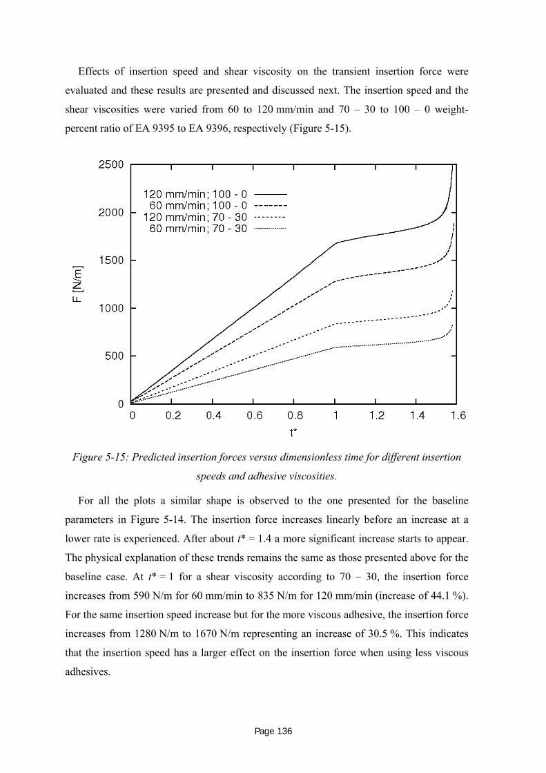
Page 136
Effects of insertion speed and shear viscosity on the transient insertion force were
evaluated and these results are presented and discussed next. The insertion speed and the
shear viscosities were varied from 60 to 120 mm/min and 70 – 30 to 100 – 0 weight-
percent ratio of EA 9395 to EA 9396, respectively ( 645HFigure 5-15).
Figure 5-15: Predicted insertion forces versus dimensionless time for different insertion
speeds and adhesive viscosities.
For all the plots a similar shape is observed to the one presented for the baseline
parameters in 646HFigure 5-14. The insertion force increases linearly before an increase at a
lower rate is experienced. After about t* = 1.4 a more significant increase starts to appear.
The physical explanation of these trends remains the same as those presented above for the
baseline case. At t* = 1 for a shear viscosity according to 70 – 30, the insertion force
increases from 590 N/m for 60 mm/min to 835 N/m for 120 mm/min (increase of 44.1 %).
For the same insertion speed increase but for the more viscous adhesive, the insertion force
increases from 1280 N/m to 1670 N/m representing an increase of 30.5 %. This indicates
that the insertion speed has a larger effect on the insertion force when using less viscous
adhesives.

Page 137
For a constant insertion speed of 60 mm/min, the insertion forces for 70 – 30 and 100 –
0 weight percent EA 9395 to EA 9396 are 590 N/m and 1280 N/m, an increase of 117 %.
Similarly, comparing the insertion forces at a higher insertion speed level of 120 mm/min,
there was an increase of 100 % (from 835 to 1670 N/m). This indicates that the insertion
force can be significantly reduced by lowering the adhesive viscosity. Furthermore, this
reduction has a higher impact for lower insertion speeds. This aspect is supported by the
results obtained for lower insertion speeds, as reported in Section 647H5.2. The insertion force
increases from 124 N/m to 389 N/m, an increase of 214 %, when the viscosity is changed
from 70 – 30 weight percent EA 9395 to EA 9396 to 100 percent EA 9395 at an insertion
speed of 5 mm/min.
Compared to the solutions derived for a Newtonian fluid in Section 648H5.1, the effect of the
insertion speed on the insertion force is weaker for the non-Newtonian, shear thinning
adhesives. There are two effects taking place simultaneously for a shear thinning adhesive
when the insertion speed is increased: on the one hand, the insertion force is increased due
to the increased insertion speed; on the other hand, the viscosity is decreased as the
increased insertion speed increases the shear rate, which for a shear thinning material
means a decrese in viscosity. The decrease in viscosity leads to a decrease in insertion
force. Both effects together result in an increase of insertion force due to insertion speed,
but at a lower rate than for Newtonian materials.
5.3.2 Results and discussion for the Pi-slot wall pressure
Another variable of interest in the development of ISF bonding processes is the pressure
distribution on the Pi-slot walls. This is important as high pressures could distort or even
damage the composite Pi-slots. A distortion of the Pi-slot walls would increase the flow
channel width and this would affect the flow of the adhesive in the flow channels.
649HFigure 5-16 illustrates the pressure distribution along the Pi-slot wall for the baseline
case at a process time shortly before the flow channels are filled completely (t* = 0.89):

Page 138
Figure 5-16: Pressure distribution along the Pi-slot wall boundary for baseline
parameters at t*=0.89.
The y-axis represents the non-dimensionalised height of the Pi-slot wall, H1*, a value of
0 is at the bottom of the Pi-slot and 1 at the top. The adhesive flow front at t*=0.89 is at a
position of about H1* = 0.91. At that position the absolute pressure is equal to ambient
pressure and the gauge pressure is zero. From this position downwards there is a linear
increase of pressure. The maximum is reached at H1*=0.13, the position of the insertion
head at that time. From this point down the pressure remains constant to the bottom of the
Pi-slot. The maximum pressure is the output variable of interest for analysing the distortion
or predicting the damage of the Pi-slots. Therefore the transient maximum pressure is
predicted with respect to different input variable effects in the following discussion.
In 650HFigure 5-17, the effect of insertion speed and shear viscosity of the adhesive on the
transient maximum pressure is shown. The maximum pressure is plotted with respect to
dimensionless time:

Page 139
Figure 5-17: Effect of insertion speeds and adhesive shear viscosities on transient
maximum Pi-slot wall pressure.
The pressure increases linearly with time until the adhesive reaches the top of the flow
channels (t* = 1). From that time onwards, the pressure increases at a low rate before
reaching an asymptotic value at a dimensionless time of about 1.3. This shows that the
flow channel width is the main parameter causing the pressure at the Pi-slot walls to
increase with respect to time. Once the adhesive flows out of the flow channels, which
means that the adhesive is not constrained by the flow channel width above the flow
channels, the transient pressure remains approximately constant.
The effect of the insertion speed and the adhesive viscosity on the pressure is similar to
their effect on the insertion force. The pressure increases with increasing insertion speed
and with increasing adhesive viscosity.
The maximum pressures for the studies cases are considered at t* = 1, taken from
651HFigure 5-17. Increasing the insertion speed from 60 to 120 mm/min at a lower adhesive
viscosity level (70 – 30) results in a pressure increase from 109 kPa to 154 kPa (increase of
41.3 %). For the higher viscous adhesives, an increase from 236 kPa to 308 kPa, which is
an increase of 30.5 %, is noticed. This trend agrees well with what has been observed from

Page 140
the insertion force data, that the insertion speed effect is greater for lower adhesive
viscosities. An increase of insertion speed leads to an increase in pressure, however this
effect is expected to be greater for a Newtonian material, as the viscosity would remain
constant. For a shear thinning fluid, however, the viscosity would decrease with increasing
insertion speed, as the shear rate would also be increased.
A similar trend is observed when comparing an increase of adhesive shear viscosities at
different insertion speed levels. Increasing the shear viscosity at the lower insertion speed
level (60 mm/min) results in a pressure increase of 117 % (from 109 kPa to 236 kPa). A
pressure increase of 100 % (from 154 kPa to 308 kPa) is noticed for the higher insertion
speed level. Again, the trend between the insertion speed and viscosity effect on pressure is
similar to the one noticed for the insertion force. The higher the insertion speed level the
less is the increase in pressure due to increasing adhesive viscosities. Here, the same
explanation can be used as in the previous paragraph. At higher insertion speeds the effect
of increasing the adhesive viscosity is smaller because the pressures are lower. The
pressures are lower as the viscosities are lower due to higher shear rates that result from the
higher insertion speed. This effect is more prevalent in materials that have a stronger shear
thinning material characteristic, i.e. their viscosity dependence on the shear rate is stronger.
This is the case for 100 – 0 EA 9395 and 70 – 30 EA 9395 to EA 9396, with the latter one
being the less shear-thinning material.
5.3.3 Insertion force and Pi-slot wall pressure dependence
Due to the similar trends observed for both the insertion force and the Pi-slot wall
pressure with respect to time, it was postulated that there could be a correlation between
those two parameters. Hence, the maximum pressure on the Pi-slot walls was compared
with the insertion force at t* = 1 and t* = 1.54 (652HTable 24). The dimensionless time of 1.54
was chosen as it is the time when the insertion plate head and the Pi-slot walls are 0.4 mm
apart in the vertical direction. For the analysed ISF process setup this distance would
represents a suitable position at which to terminate the motion of the insertion plate, due to
the use of spacers to align the insertion plate within a required tolerance inside the Pi-slot.
(A detailed discussion about the use of spacers is presented in sub-Section 653H6.4.1).
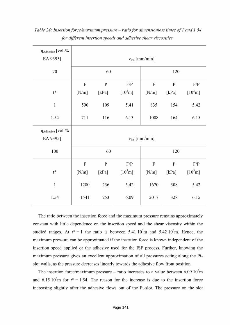
Page 141
Table 24: Insertion force/maximum pressure – ratio for dimensionless times of 1 and 1.54
for different insertion speeds and adhesive shear viscosities.
ηAdhesive [vol-%
EA 9395] vins [mm/min]
70 60 120
t*
F
[N/m]
P
[kPa]
F/P
[103m]
F
[N/m]
P
[kPa]
F/P
[103m]
1 590 109 5.41 835 154 5.42
1.54 711 116 6.13 1008 164 6.15
ηAdhesive [vol-%
EA 9395] vins [mm/min]
100 60 120
t*
F
[N/m]
P
[kPa]
F/P
[103m]
F
[N/m]
P
[kPa]
F/P
[103m]
1 1280 236 5.42 1670 308 5.42
1.54 1541 253 6.09 2017 328 6.15
The ratio between the insertion force and the maximum pressure remains approximately
constant with little dependence on the insertion speed and the shear viscosity within the
studied ranges. At t* = 1 the ratio is between 5.41 103m and 5.42 103m. Hence, the
maximum pressure can be approximated if the insertion force is known independent of the
insertion speed applied or the adhesive used for the ISF process. Further, knowing the
maximum pressure gives an excellent approximation of all pressures acting along the Pi-
slot walls, as the pressure decreases linearly towards the adhesive flow front position.
The insertion force/maximum pressure – ratio increases to a value between 6.09 103m
and 6.15 103m for t* = 1.54. The reason for the increase is due to the insertion force
increasing slightly after the adhesive flows out of the Pi-slot. The pressure on the slot

Page 142
walls, however, remains approximately constant as shown in 654HFigure 5-17. The reason for
the slight force increase seems likely to be caused by the increase in shear forces along the
insertion plate walls due to an area increase as the insertion plate continues to move down,
which would appear even after the adhesive flows out at the top of the Pi-slot. The
pressure, however, is not affected by this increase. Therefore, the ratio between the
insertion force and pressure has to increase after the adhesive flows out of the flow
channels.
This finding is particularly important for the design of the composite Pi-slot. If the
insertion force is known, the maximum pressure acting on the Pi-slot walls can be
approximated. For the considered parameter range and assuming a spacer diameter of
0.4 mm, this pressure could be estimated by multiplying the insertion force by a factor of
6.15 103m. Having a method to predict the pressure is important because of the difficulty
of measuring it experimentally.
To show how the dependence between the insertion force and Pi-slot wall pressure is
affected by the process time, the force-pressure-ratio is plotted against dimensionless time
in 655HFigure 5-18 for simulations varying in the insertion speed and the adhesive viscosity.

Page 143
a) b)
c) d)
Figure 5-18: Effect of the insertion speed and the adhesive viscosity on the insertion
force/maximum Pi-slot wall pressure – ratio with respect to dimensionless time.
The transient ratio initially shows an increase from about 5.3 103m to 5.4 103m because
the shear forces do not contribute to the insertion force as they do after t* = 0.05, when the
velocity profile and hence velocity gradients within the flow channels have developed. The
pressure, however, is not affected by this process. Until the flow channels are filled
entirely, the ratio remains approximately constant. An increase can be observed after
t* = 1.2. The shear forces at the insertion plate lead to an increase in insertion force but not
in pressure on the Pi-slot walls. The insertion terminates when the insertion plate can no
longer move further down, this happens when the insertion plate head and the Pi-slot
bottom boundaries become very close to each other, leading to a significant increase in the
insertion force. The flow velocities within the narrow gap between the boundaries become
very large, resulting in high pressures being required under the plate to overcome the
resistance to the flow with a consequent rapid increase in insertion force. However, the
pressure within the flow channels and hence the Pi-slot wall pressure hardly increases
when this occurs as only a small amount of adhesive can still be squeezed through the

Page 144
narrowing gaps between the insertion plate head and the Pi-slot bottom. This is the same as
was shown for a different case in 656HFigure 5-9.
657HFigure 5-18 can be used to estimate the maximum pressure at the Pi-slot walls for
different process times if the insertion force is known. When designing an ISF process, the
total process time would normally be known in advance as the necessary initial adhesive
amount is known. Assuming there is a nominated intended stop of the insertion plate’s
motion, the maximum pressure at the Pi-slot walls at that time could be estimated.
Thus, the maximum pressure at the Pi-slot walls for perfectly aligned cases can be
estimated for the entire ISF process. This is valid for the considered insertion speed range
(60 – 120 mm/min) and adhesive viscosities (70 – 30 and 100 – 0 weight percent EA 9395
to EA 9396) for given insertion forces. However, based on the arguments presented here it
is expected that the form of the relationship between the variables would also be more
generally applicable.
5.3.4 Insertion force and Pi-slot wall pressure for different adhesive material models
As shown in 658HFigure 4-23 on page 659H113 (sub-Section 660H4.4.5) the shear viscosity versus
shear rate data can be more accurately represented by the five parameter rational model,
especially at higher shear rates. Thus, the prediction of the insertion force with respect to
time was predicted again applying this model. The resulting insertion forces were
compared with those predicted using the power law model for an insertion speed of
60 mm/min and an adhesive viscosity of to 70 – 30 weight percent EA 9395 to EA 9396.
Other input parameters were the standard set used above. The resulting insertion forces are
plotted in 661HFigure 5-19:

Page 145
Figure 5-19: Effect of the adhesive material model on the predicted transient insertion
force for two adhesive viscosities.
The plotted graphs have a similar shape to those previously seen. A linear insertion
force increase is followed by an increase at a lower rate after the flow channels are filled
entirely before a significant increase is noted when the insertion plate head approaches the
Pi-slot boundary. However, the differences resulting from the different viscosity models
are quite substantial, as is expected given that the Power law models provide a rough
approximation of the measured viscosities.
The predictions were considered at t* = 1. At the lower shear viscosity level of 70 – 30,
the insertion forces are predicted as 590 N/m and 993 N/m for the power law and the five
parameter rational model, respectively. For the higher shear viscosity level (100 – 0) the
insertion forces are 1280 N/m and 2232 N/m for the power law and the five parameter
rational model, respectively.
The reason for these differences can be explained with the different shear viscosities
within the flow domain for the different adhesive models. The viscosity fields for a 70 – 30
mix and an insertion speed of 120 mm/min at t* = 0.21 are illustrated for the power law
and the 5 parameter rational model in 662HFigure 5-20.

Page 146
a) b)
Figure 5-20: Shear viscosity field at an insertion speed of 120 mm/min at t* = 0.21 for a)
the power law model and b) the five parameter rational model.
The measured shear viscosity with respect to shear rate as presented in sub-
Section 663H4.4.2 is illustrated again in 664HFigure 5-21.
Figure 5-21: Measured adhesive viscosity with respect to shear rate for three samples of a
70 – 30 mix of EA 9395 to EA 9396.

Page 147
At an insertion speed of 120 mm/min, which is high for the in this study considered
insertion speed ranges, the shear rates are high, therefore it is important to consider the
lower limits of the viscosity field, as the viscosity decreases with increasing shear rates.
The problems in using the power law model are evident in Figure 5-20, in which there
are regions where the adhesive viscosity is between 0 and 20 kg m-1s-1 in contrast with the
measured adhesive viscosities in Figure 5-21, which shows no values below 20 kgm-1s-1. In
contrast, the results of simulations using the five parameter model are consistent with the
measured results across the full range of shear rates.
Due to the fact that the predictions at higher insertion speed were inaccurate when the
Power law model was used for the adhesive, the maximum pressure was predicted at the
Pi-slot walls again using the adhesive viscosities predicted by the five parameter model for
t* = 1 in 668HTable 25.
Table 25: Maximum pressure at Pi-slot walls for five parameter rational adhesive viscosity
models at t* = 1 for different adhesive viscosities and insertion speeds.
ηadh [weight-percent EA 9395 to
EA 9396]
vins [mm/min]
70 – 30 100 – 0 60 120
Pmax [kPa]
at t* = 1
X X 184
X X 513
X X 348
X X 748
The physical effect of insertion speed and adhesive viscosity on the pressure is as
discussed previously, 669HTable 25 provides the quantitative values of using the five parameter
rational model. To show that the insertion force – Pi-slot wall – pressure dependence
which was derived is not affected by the adhesive material model, the force/maximum Pi-
slot wall pressure-ratio is plotted with respect to dimensionless time for the 70 – 30 mix
and 100 % EA 9395 in 670HFigure 5-22.

Page 148
Figure 5-22: Effect of the adhesive viscosity (70-30 left, 100-0 right hand side) on the
insertion force/maximum Pi-slot wall pressure – ratio with respect to dimensionless time,
predicted applying the five parameter rational model.
The dependence between the insertion force and the maximum Pi-slot wall pressure
presented in 671HFigure 5-22 is identical to that presented in 672HFigure 5-18. Hence, the maximum
pressure and also the pressure distribution along the entire Pi-slot can be estimated if the
insertion force is known, providing important information for the support of Pi-slot design
for ISF processes.
As the effect of the adhesive material model on the output variables is quite significant
quantatively, and in addition having shown that the five parameter model predicts the
adhesive viscosity more accurately for high shear rates, from the following sub-
Section 673H5.3.5 onwards, the predictions shown were obtained using the five parameter
rational material model instead of the power law model.
5.3.5 Effect of insertion speed on specific insertion force and Pi-slot wall pressure
Here the effect of the insertion speed on the insertion force and the maximum pressure
acting along the Pi-slot walls is examined for the entire insertion speed range considered.
The adhesive viscosity (70 – 30 mixture) was represented by the five parameter rational
model and the results presented are compared at one specific time (t*=1). The specific
insertion force and the maximum pressure along the Pi-slot wall are shown with respect to
insertion speed in 674HFigure 5-23:

Page 149
a) b)
Figure 5-23: Insertion speed effect on a) specific insertion forces and b) maximum
pressures on the Pi-slot walls at t* = 1 and a 70 – 30 adhesive mix.
A linear fit applied to the force and maximum pressure agrees well with the numerical
predictions. The agreement between the linear fit and the values for the insertion forces is
an over four values averaged 8.6 N according to the root square mean deviation (1.6 kPa
for the pressure values). Hence, to predict the specific insertion force using a 70 – 30
weight-percent mixture of EA 9395 to EA 9396 a linear relation of the form
24932415 .v.F insspec += with 5 < vins < 120 mm/min (5-9)
can be used and the maximum pressure can be predicted as
07698272 .v.p insmax += with 5 < vins < 120 mm/min. (5-10)
The linear relation between the maximum pressure and the insertion speed as shown in
equation 675H(5-10) results from the linear relation between the insertion force and the insertion
speed as shown in equation 676H(5-9). This is because the maximum pressure depends on the
insertion force, which was presented in sub-sections 677H5.3.3 and 678H5.3.4. So the relation
between the insertion force and the insertion speed is considered in more depth, as findings
can also be applied to explain the dependence between the maximum pressure and the
insertion speed.
The adhesive flow under consideration is a low Re flow (Re < 1). For these types of
flow the drag force is expected to be a function of the velocity (Munson, 2006). The drag
force on the insertion plate in the considered problem is the insertion force, consisting of
viscous and pressure forces. Both are linearly related to the insertion speed, so it would be
expected that the insertion force is a linear function of the insertion speed, which is the
case, as seen from equation 679H(5-9). The gradient in equation 680H(5-9) results from the adhesive

Page 150
viscosity and the dimensions of the insertion plate and the Pi-slot. The maximum pressure
therefore is also linearly dependant on the insertion speed.
The linear fit is only valid where the insertion force is dependent on viscous and
pressure forces arising from the insertion process, hence when the insertion plate is in
motion. This was also applied in the force balance of the analytical model (Section 5.1). At
initiation of the insertion process, non-linearities are likely to exist and hence equations
(5-9) and 675H(5-10) may not be valid. According to equation 680H(5-9), an insertion speed of 0
does not result in an insertion force of 0, as is physically expected. More analysis would be
needed to clarify events at very low insertion speeds. As the bonding process time is
expected to be within seconds, however, insertion speeds in the range smaller than
60 mm/min are considered to be of minor importance. Given this requirement, a further
analysis at very low insertion speeds, typically smaller than 2 mm/min, would be
considered as unjustified.
It also is highly likely that at higher insertion speeds than those under consideration
other forces become dominant and again non-linearities are expected.
5.4 Insertion Squeeze Flow at High Insertion Speeds with Different Insertion Head Shapes
In sub-Section 682H3.5.1 it was indicated that the insertion head shape was another
parameter to be varied during this research. The term “insertion head shape” specifies the
design of the bottom of the insertion plate that is inserted into the Pi-slot. The insertion
head shape used up until this point was rectangular (Sections 683H5.1 to 684H5.3).
Three alternative insertion head shapes were analysed. Two of them were tapered,
varying in the length of the taper and consequently in the taper angles, and one was
rounded. These are illustrated in 685HFigure 5-24 together with the studied rectangular shape:

Page 151
R 2
Shape 3Shape 1
1
5
1
Shape 2
3
Shape 4
5R 2
Shape 3
R 2
Shape 3Shape 1
1
5
Shape 1
11
555
1
Shape 2
3
1
Shape 2
33
Shape 4
5
Shape 4
55
Figure 5-24: Insertion head shape variations.
Given that the mechanical effectiveness of the bonded joints is known to be influenced
by the shape of the insertion head shape, the effect of different head shapes on the insertion
forces and slot pressures were examined for the higher insertion velocity of 60 mm/min,
which is more like the speed that would be used in practical applications.
The dimensions and process parameters were as presented in Table 22. The adhesive
viscosity was a 70 – 30 weight percent EA 9395 to EA 9396, modeled using the five
parameter rational model. The adhesive was initially applied at 125 volume-percent, noting
that this means the absolute volume varies for the different head shapes, which results in
different initial adhesive heights.
In 687HFigure 5-25 the insertion force is plotted with respect to time for the three alternative
insertion head shapes and the already presented case when the insertion head shape is
rectangular.

Page 152
Figure 5-25: Predicted transient insertion force for different insertion head shapes.
The insertion force increases linearly for all cases until the flow channels are filled, and
this is followed by an increase at a lower rate. When the insertion plate approaches the Pi-
slot a significant increase occurs. This occurs earliest for shape 3, then for shape 4 and
finally for shapes 2 and 1. These differences result from the differences in insertion head
shapes and in the consequential different absolute initial adhesive amounts. For example in
the case of shape 3 less adhesive is necessary because the insertion plate and the Pi-slot can
approach each other more closely compared to the other cases where more “free volume”
remains in the final bonding position.
From 688HFigure 5-25, it can also be seen that it is only for shape 4 that the insertion force
starts increasing immediately. For all other cases a delay is observed. This delay can be
explained by illustrating the initial adhesive distribution within the flow channels as shown
in 689HFigure 5-26, which also indicates the differences in the initial adhesive amount.

Page 153
Figure 5-26: Initial adhesive distribution for the four investigated head shapes. Adhesive is
represented by the red colour, air is blue.
It can be seen that different parts of the insertion plate are in contact with the adhesive.
For the two tapered shapes only the flat bottom touches the adhesive initially. The adhesive
does not start to flow into the flow channels until the area between the tapered head and the
Pi-slots is filled. When this area is filled with adhesive, the insertion force begins to
increase. Thus the delay observed in 690HFigure 5-25 is characterised as the time to fill the area
between the tapered walls of the insertion plate and the Pi-slot walls. Similarly, for the
rounded case a delay is observed that is smaller than the one for the tapered heads. The
delay is caused by the filling of the area between the rounded parts of the insertion plate
and the Pi-slot. As this area is smaller than the area for the tapered insertion plates the
filling time and thus the delay is shorter. No delay is observed for the rectangular shape as
the adhesive flows into the flow channels directly.
The graph shows that the rounded shape (shape 3) results in the highest insertion forces.
This is due to the fact that in case of shape 3 the insertion plate can descend further than
shape 4 and as a result the insertion plate and the Pi-slot would touch later. The lowest
insertion forces occur for the longer tapered head shape (shape 1). The main reason for this
is that the pressure that acts within the Pi-slot bottom is smaller compared to the rounded
or rectangular shape. The comparable pressure is smaller for the tapered shape as more
space is provided between the insertion plate head and the Pi-slot bottom. Thus the
pressure force component of the drag force is smaller resulting in the lowest total insertion
force observed.

Page 154
For the maximum pressure at the Pi-slot wall variation with flow time, the different
insertion head shapes have similar effects to those observed for the transient insertion
forces. This can be seen in 691HFigure 5-27.
Figure 5-27: Transient maximum pressure along the Pi-slot wall with respect to different
insertion head shapes.
692HFigure 5-27 presents the transient local maximum pressure value along the Pi-slot. The
local maximum pressure can be found as presented in 693HFigure 5-16 on page 694H138 at the edge
of the Pi-slot wall. The maximum pressure increases roughly linearly with time. When the
adhesive reaches the top of the flow channels the transient pressure increases at a lower
rate as the resistance towards flowing of the adhesive through the flow channel widths
disappears above the top of the Pi-slots.
The highest pressures acting along the Pi-slot walls are detected for the same case as the
highest drag coefficients, this is for shape 3. As the insertion plate can move down further
than the rectangular plate and also provides less space compared to the two tapered heads,
the pressure within the Pi-slot is considerably larger. As found for the insertion force and
for the same reasons, the lowest pressures are detected due to the reasons described for the
insertion forces for shape 1.

Page 155
Finally, the dependence between the insertion force and the Pi-slot wall pressure was
evaluated and is presented. Dividing the insertion force by the maximum Pi-slot wall
pressure results in the following factor for the investigated head shapes if the adhesive flow
front is within the 0.5 mm wide region of the flow channel:
− Shape 1: 5.35 103m;
− Shape 2: 5.38 103m;
− Shape 3: 5.50 103m;
− Shape 4: 5.41 103m.
Again, if the insertion force is known the maximum pressure can be approximated,
providing a useful approach for the design of Pi-slot components to be used for ISF.
5.5 Experimental Study of ISF at High Insertion Speeds
The experimental approach used was as described in Chapter 695H3.6. The insertion force at
constant insertion speed was measured with respect to time on a 10 kN Instron universal
testing rig. Test specimen length in the longitudinal direction (z-direction) were 282 mm
and 283 mm for the insertion plates and the Pi-slots, respectively, with all other dimensions
being according to baseline parameters. The insertion plate head shapes were rounded
(R=2.5 mm) and tapered (2 mm vertical, 5 mm horizontal), according to 696HFigure 5-24, and
two measurements per head type were conducted. To connect the insertion plate to the
cross head of the test rig, the insertion plate was clamped to a rigid steel angle. The other
end of the steel angle was clamped to the cross head of the testing machine. This can be
seen in 697HFigure 5-28, where the experimental test set up is illustrated; the same image is
shown in 698HFigure 3-14.

Page 156
Figure 5-28: Test setup for the second set of experiments to measure the insertion force
during an ISF bonding process.
For three of the experiments two wires were used to ensure that good alignment was
maintained between the insertion plate and the Pi-slot. For the last experiment, the number
of wires was increased to three.
The insertion force was plotted with respect to time for the experiments for the rounded
and tapered insertion plate heads in 699HFigure 5-29. The measurements were conducted at an
insertion speed of 60 mm/min and an adhesive mixing ratio of 70 – 30 EA 9395 to
EA 9396. Also shown in 700HFigure 5-29 are the numerical results for the rounded and the
short tapered insertion head for a total flow channel width of 1 mm.

Page 157
Figure 5-29: Measured insertion forces plotted against dimensionless time for the rounded
and the tapered insertion plate heads in comparison to numerical results for the same
cases with a total flow channel width of 1 mm.
Before analysing the differences between the numerically predicted and the
experimentally measured insertion forces, the general shape of the insertion force is
discussed, followed by a discussion of discrepancies detected between two experiments for
the same set, as indicated by the error bars. After this analysis, a comparison between the
numerical results and the experiments is made.
Two insertion force regions are noticed for both insertion heads: in the very beginning,
the measured and predicted insertion forces are only slightly above zero, which is when the
insertion plate heads touches the adhesive. The little force detected results from the filling
of the area around the insertion plate radius and the tapered ends of the insertion plate,
respectively, with adhesive, before the adhesive is displaced into the flow channels (0 –
0.2 s). In the experiments, this increase might also correspond to the compaction of the
initially uneven adhesive surface. The second region shows an insertion force increase at a
higher rate until the adhesive eventually flows out of the flow channels at t* = 1, which
was not achieved for all of the experiments.
From observations of the previous set of experiments as well as of numerical results for
insertion forces at constant insertion speed a plateau-like region would be expected to
occur before a final significant increase indicates the touch between the insertion plate and
the Pi-slot. However, this is not observed here. Analysis of the specimens indicated that the
adhesive in some cases did not fill both flow channels entirely. For the experiments in
which two spacers were used, the adhesive flowed out in the middle on one side and at the
ends on the other side of the insertion plate. This adhesive distribution implies a bending of
the insertion plate. A possible explanation is that the clamping of the insertion plate to the

Page 158
steel angle imposes an angular misalignment. Due to the spacers that are wrapped around
the head of the insertion plate, the angular misalignment might lead to a bending around
the spacers – a similar bending effect as experienced during a three point bending test.
Calculations of the loads necessary to bend the insertion plate show that a loading of less
than 10 N/m would be sufficient to bend the insertion plate (sub-section 701H6.4.2). This
possible explanation was supported by two further observations; first, the adhesive
distribution is the same for all three experiments conducted with two spacers, being that
the insertion plate side where the adhesive flows out at the ends faces the angle. Second,
the adhesive is distributed evenly along the joint for the last conducted experiment when
three wires were used. The Pi-joint bonded with three spacers is shown in 702HFigure 5-30.
Figure 5-30: A Pi-joint after bonded applying the ISF process at constant speed; three
spacers were used to align the insertion plate in the Pi-slot.
Considering 703HFigure 5-29 again, possible explanations are given for the differences
between the two conducted experiments, as indicated by the error bars:
− Variation of joint dimensions may lead to differences in flow channel widths,
− weighing of four different components of the adhesive can lead to different
adhesive viscosities, calculated as 0.545 % by uncertainty analysis (Holman, 1994)
− due to manual mixing a proper distribution of the components cannot be
guaranteed,

Page 159
− different amounts of different adhesive components may remain in the mixing
devices leading to different adhesive viscosities.
The last two uncertainties cannot be estimated, but they are expected to be within a
similar range for each experiment because same procedures were applied for every
experiment.
The width of the flow channels is the parameter that mainly would affect the insertion
forces. More discussion on the point that the flow channel width is the main cause for
discrepancies is provided in the following comparison between the numerical and
experimental results.
Comparing the insertion forces at t* = 1, these were found to be an average of 732 N/m
for the rounded insertion head from the experiments, but 1044 N/m from numerical
predictions. For the tapered insertion head (shape 2) the measured insertion force at t* = 1
was 621 N/m, while the numerically predicted one was 985 N/m. This is a difference of
30 % for the rounded and of 37 % for the tapered head.
The total flow channel width for the rounded insertion plate varied between 1.07 mm
and 1.38 mm, whereas the one for the tapered insertion plate head resulted in a variation
between 0.92 mm and 1.42 mm. As mentioned above, this was suspected to be the main
reason for the differences experienced between the numerical and experimental results.
Hence, two more numerical simulations were setup matching the smallest and the largest
resulting flow channel widths. The insertion plate widths and the Pi-slot widths were setup
according to those used for the most extreme cases appearing in the experiments, so that
the insertion plate width for the first simulation was 5.14 mm and the Pi-slot width was
6.06 mm, and for the second simulation these were 4.85 mm and 6.27 mm. The simulations
were conducted for the tapered insertion head. The results are shown in 704HFigure 5-31:

Page 160
Figure 5-31: Numerically predicted insertion forces for a narrow and a wide total flow
channel width compared to experimentally measured insertion forces, plotted with respect
to dimensionless time for the tapered insertion head shape.
It was found that the numerical predictions of the insertion force for the widest and for
the narrowest flow channel width derived from the experiments envelope the insertion
force measurements. This shows that the numerical and the experimental insertion forces
do not contradict. Hence, the differences experienced and shown in 705HFigure 5-29 clearly
result from the different dimensions used for the experiments and the numerics.
For the rounded design, this strongly suggests that the discrepancies experienced are
also caused by the different flow channel widths for the experiments and numerical
simulations. The flow channel widths in those experiments were larger than 1 mm, varying
between 1.07 mm and 1.38 mm, thus being expected to predict lower insertion forces than
those predicted when the flow channel width is 1 mm.
The conclusions obtained from the above presented experiments are as follows:
− The test rig concept should be designed to guarantee a symmetrical loading of the
insertion plate so that bending of the bonding partners is circumvented which in
general may occur at low loadings;

Page 161
− the adhesive amount applied initially should be at least 50 weight-percent in excess
of the necessary amount if the insertion head shape is rounded; this becomes even
more important when the accuracy of the component’s dimensions are unknown;
the usage of optical measurement devices is suggested, and this would also support
the selection of spacer diameters;
− from the conducted experiments it appears that three spacers or more along a
280 mm long joint are necessary to ensure the desired adhesive distribution;
however it is believed that the test rig setup had inadequacies that led to the
unequal distribution so that the number of spacers most likely can be reduced if the
test rig concept enables a symmetrical loading of the insertion plate during
clamping;
To sum up, there was a discrepancy of about 30 % detected between the measured and
predicted insertion forces, which was shown to be due to different flow channel widths,
and numerical predictions from two further simulations did not contradict the insertion
forces measured. It was difficult to conduct experiments that agree entirely with the
numerical setup so that results can be used to conduct correct comparisons.
5.6 Summary
In this chapter analytical and numerical predictions for insertion forces and velocity
distributions within the flow channels were compared for a Newtonian ISF process and
showed good agreement. Insertion force predictions also agreed well with experimental
results obtained for ISF conducted at low insertion speed. A further output variable that
was predicted by the numerical model is the pressure distribution along the Pi-slot walls,
which is maximum at the root of the Pi-slot. How this pressure varies with the insertion
force was also found and specifed. The insertion force and the maximum Pi-slot wall
pressure were found to vary linearly with the insertion speed. Experiments were also
conducted at high insertion speeds with the insertion force being measured. Discrepancies
between the experimentally measured insertion forces and the numerically predicted
insertion forces were found and attributed to differences between the setups, which were
different in terms of flow channels width. Insertion force predictions for the widest and
smallest flow channel width did not contradict with experimental insertion forces.
Suggestions were provided for the conduction of an ISF process in practice.

Page 162
6 Insertion Squeeze Flow considering Lateral Misalignment
In Chapter 706H6 the dimensional variations that are possible during ISF, and which
consequently affect adhesive flow, are introduced in Section 707H6.1. Causes of lateral
misalignments are presented in Section 708H6.2. Lateral misalignment effects on the adhesive
flow are evaluated numerically in Section 709H6.3. Procedures are then proposed to estimate a
minimum necessary initial adhesive amount to ensure complete flow channel filling, with
reasons for asymmetrical flow during ISF being discussed. Chapter 710H6 concludes with an
estimation of the number of spacers that should be used to ensure minimum flow channel
widths during insertion.
6.1 Possible Misalignments during Insertion
Misalignments that might occur during ISF are illustrated in 711HFigure 6-1:
x
y
x
y
x
y
x
z
x
z
x
z
z
y
z
y
z
y
a) b) c)
Figure 6-1: Possible misalignments that can occur during ISF: a) Lateral (x-axis) and
angular misalignment around z-axis; b) Angular misalignment around y-axis; c) Angular
misalignment around x-axis.

Page 163
Misalignments can be either angular or lateral. The two flow channels are affected by
lateral misalignment relative to the x-axis and by angular misalignment around the y-axis
and z-axis (712HFigure 6-1 a) and b)). Angular misalignment around the x-axis (713HFigure 6-1 c)),
however, would not necessarily affect the flow channel width, but might cause significant
adhesive flow in the z-direction.
Lateral misalignment is expected to be the most common dimensional variation and
hence is discussed in depth in the following Sections 714H6.2 and 715H6.3.
6.2 Causes of Lateral Misalignment
The nominal dimensions of a Pi-slot cross section typically used for ISF are presented
in 716HFigure 6-2:
x
y
x
y
x
y
60.5
2.5
R3
12
R3
35
34
70
3.50.5
3
x
y
x
y
x
y
60.5
2.5
R3
12
R3
35
34
70
3.50.5
3
Figure 6-2: Key dimensions that define the Pi-slot structure and that are specified in the
MoJo project (MoJo, 2007).
Of particular interest for the analysis of ISF bonding is the Pi-slot height (35.5 mm),
which is referred to as H1 throughout the studies, and the Pi-slot width (6.0 mm), also
referred to as 2b. The counter part to be bonded with the Pi-slot is the insertion plate. Its
nominal width (2a) is 5.0 mm. When the insertion plate is aligned exactly symmetrically
between the Pi-slot walls, the resulting flow channel widths (δ) on both sides of the
insertion plate are equal and 0.5 mm.

Page 164
However, in practice a number of issues have lead to dimensional variations in Pi-joints.
These dimensional variations are caused by
− manufacturing tolerances of the composite components,
− process induced distortions during ISF and
− misalignments between the composite bonding partners during insertion of the
insertion plate.
All of these lead to flow channel width variations and consequently affect the adhesive
flow during ISF. As the quality of a Pi-joint is significantly influenced by the bondlines, an
improper adhesive distribution would have a significant impact on the Pi-joint quality.
6.2.1 Manufacturing tolerances
In Mojo (2007), various dimensional tolerances of composite laminates have been
defined. 717HTable 26 lists those that are relevant for the current study:
Table 26: Manufacturing tolerances as specified in the Mojo project (MoJo, 2007) and the
resulting flow channel widths.
Feature Nominal
length [mm]
Minimum
tolerance [mm]
Maximum
tolerance [mm]
Expected
range [mm]
Insertion plate
width
5.0 -0.2 0.2 4.8 – 5.2
Pi-slot width 6.0 0 0.2 6.0 – 6.2
Minimum total
flow channel width
δmin = 6.0 – 5.2 = 0.8
Maximum total
flow channel width
δmax = 6.2 – 4.8 = 1.4
From the manufacturing tolerances a total flow channel width range was derived. An
additional tolerance of interest is the straightness or flatness deviation, illustrated in 718HFigure
6-3:

Page 165
h1
h2
Figure 6-3: The permissible flatness deviation as defined in Mojo (2007).
No definition is provided of a length scale over which the permissible flatness
deviations h1 and h2 are defined in (MoJo, 2007). Hence, for the purpose of the present
work we assumed the length scale to be defined as the approximate length of the side
panels of the A-level demonstrator (MoJo, 2009), 1320 mm.
6.2.2 Spring-in effect
The Pi-joint under consideration can be approximated by two back to back flanged
laminates (Liu, 2009). A well known distortion of flange laminates – also referred to as the
spring-in effect – might occur after de-moulding due to thermal contractions as well as
resin cure shrinkage in both the in-plane and through-thickness directions. Less contraction
is expected in the circumferential direction, so that consequently the flange angle tends to
close (Liu, 2006). 719HFigure 6-4 illustrates the Pi-joint representation by two back to back
flanged laminates and the expected deflection of the laminates.
Figure 6-4: Two back-to-back flanged laminates approximating the Pi-slot for the
description of the spring-in effect (Liu, 2009).
It is believed, however, that a flanged laminate’s distortion would in the present case
actually result in a slight opening-up. This is mainly due to the lay-up of the Pi-slot, which
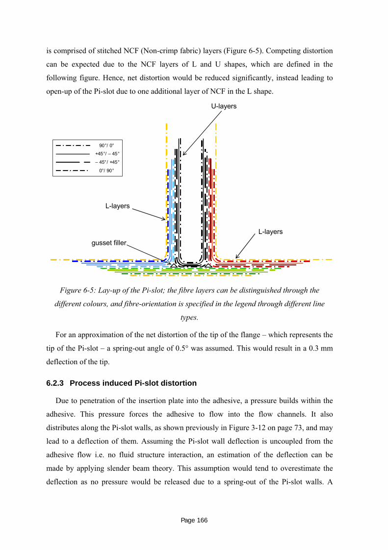
Page 166
is comprised of stitched NCF (Non-crimp fabric) layers (720HFigure 6-5). Competing distortion
can be expected due to the NCF layers of L and U shapes, which are defined in the
following figure. Hence, net distortion would be reduced significantly, instead leading to
open-up of the Pi-slot due to one additional layer of NCF in the L shape.
90°/ 0°
+45°/ – 45°
– 45°/ +45°
0°/ 90°
L-layers
gusset fillerL-layers
U-layers
Figure 6-5: Lay-up of the Pi-slot; the fibre layers can be distinguished through the
different colours, and fibre-orientation is specified in the legend through different line
types.
For an approximation of the net distortion of the tip of the flange – which represents the
tip of the Pi-slot – a spring-out angle of 0.5° was assumed. This would result in a 0.3 mm
deflection of the tip.
6.2.3 Process induced Pi-slot distortion
Due to penetration of the insertion plate into the adhesive, a pressure builds within the
adhesive. This pressure forces the adhesive to flow into the flow channels. It also
distributes along the Pi-slot walls, as shown previously in 721HFigure 3-12 on page 722H73, and may
lead to a deflection of them. Assuming the Pi-slot wall deflection is uncoupled from the
adhesive flow i.e. no fluid structure interaction, an estimation of the deflection can be
made by applying slender beam theory. This assumption would tend to overestimate the
deflection as no pressure would be released due to a spring-out of the Pi-slot walls. A

Page 167
process induced deflection of the Pi-slot wall due to insertion pressure is illustrated in
723HFigure 6-6.
x
y
Pi-slot
Adhesive at specific
flow front
Resulting pressure
distribution px(y)
Deflected Pi-slot
due to acting pressure
Changed flow
channel width
x
y
Pi-slot
Adhesive at specific
flow front
Resulting pressure
distribution px(y)
x
y
x
y
Pi-slot
Adhesive at specific
flow front
Resulting pressure
distribution px(y)
Deflected Pi-slot
due to acting pressure
Changed flow
channel width
Deflected Pi-slot
due to acting pressure
Changed flow
channel width
Figure 6-6: Illustration of the Pi-slot wall deflection due to insertion pressure leading to a
broadening of the flow channel; the pressure is caused by the flow of the adhesive.
A cantilever beam model was derived to estimate the Pi-slot wall distortion, with the
boundary condition at the bottom being fixed into the wall as a cantilever. An illustration
of this model can be seen in 724HFigure 6-7.

Page 168
x
y
Pi-slot
Adhesive at specific
flow front
Resulting pressure
distribution px(y)
x
y
x
y
Pi-slot
Adhesive at specific
flow front
Resulting pressure
distribution px(y)
Figure 6-7: Beam model to approximate the Pi-slot wall deflection; boundary conditions at
the bottom of the Pi-slot is fixed into the wall as a cantilever.
An investigation of the effect of Pi-slot wall deflection on adhesive flow was conducted
and is reported on in Section 725H7.3. There, the problem is presented assuming a coupling
between the adhesive flow and the Pi-slot deflection, hence taking into account a fluid
structure interaction.
6.3 Lateral Misalignment Effect on the Adhesive Flow
In Section 726H6.2 the causes of lateral misalignment in the adhesive’s flow during the ISF
processes were discussed. Flow channel widths vary in laterally misaligned insertions so
that an asymmetric adhesive distribution may be experienced.
This would result in a deterioration of the Pi-joint quality once the adhesive in the flow
channels cures and the bondlines are built. Different flow channel widths and an expected
adhesive distribution are demonstrated in 727HFigure 6-8.

Page 169
δ 1
δ 2δ1≠ δ2
Insertion plate
Pi-slot
Adhesive
x
z
δ2
δ1
x
y
δ 1
δ 2δ1≠ δ2
Insertion plate
Pi-slot
Adhesive
x
z
x
z
δ2
δ1
δ2
δ1
x
y
x
y
Figure 6-8: Schematic illustration of lateral misalignment resulting in different flow
channel widths δ1 and δ2,, shown as a top- and a cross-sectional view.
The results of how lateral misalignment affects the adhesive flow within the flow
channels are discussed first, and ISF-specific dimensionless parameters are derived. In sub-
Section 728H6.3.1.2 the emphasis is on the sensitivity of lateral misalignment effects on the
insertion speed and in sub-Section 729H6.3.1.3 on the adhesive viscosity. The initial adhesive
amount effect on the adhesive distribution was analysed and results are presented in sub-
Section 730H6.3.1.4. Furthermore, the effect of the total flow channel widths on adhesive flow
is considered. The last two sections of this chapter deal with the analysis of causes for
asymmetrical adhesive flow (sub-Section 731H6.3.2) and with the effect of insertion head shape
on the adhesive flow.
6.3.1 Results and discussion
6.3.1.1 Effect of the flow channel width ratio
The results presented were obtained for insertion speeds of 60 mm/min and adhesive
viscosities for the 70 – 30 weight percent EA 9395 to EA 9396 and using the five
parameter rational model discussed in sub-Section 732H4.4.5. The initially applied adhesive
volume was 125 volume-percent of the volume to be filled. The dimensions of the joint

Page 170
were 5.0 mm and 6.0 mm for the insertion plate and the Pi-slot width, respectively,
resulting in a total flow channel width of δtotal = 1.0 mm. The asymmetry of the two flow
channels is represented by the ratio between the narrow (N) and the wide (W) flow channel
widths, it is referred to as ξ=N/W.
Firstly the adhesive distribution for a perfectly aligned case is shown, for this case the
resulting flow channel widths are 0.5 mm:
Figure 6-9: Numerically predicted fill heights with respect to dimensionless time for a
perfectly aligned insertion represented by 826 points within an interval of 1.6
dimensionless time units t*.
In 733HFigure 6-9 H* is defined as the flow front c plus the initial adhesive height H0
divided by the total Pi-slot height H1 and is plotted against dimensionless time. We defined
this parameter as the fill height:
1HHcH 0+
=* (6-1)
The definition of c, H0 and H1 can be found in 734HFigure 3-8 on page 735H69. At a
dimensionless time t*=1 the flow front reaches the top of the slot, hence H* is 1. As
expected, for an insertion without misalignment the flow fronts in both channels are

Page 171
identical. The initial adhesive amount of 125 volume percent is represented for this
particular geometry by an initial fill height of 0.25.
In 736HFigure 6-10 the effect of laterally misaligned cases on the fill height is shown with
respect to time. Results of three simulations are presented where the flow channel widths
were as follows: 0.5 mm on both sides of the insertion plate equivalent to the case
presented in 737HFigure 6-9; 0.4 mm and 0.6 mm, thus a misaligned case of 0.1 mm; and finally
0.3 mm and 0.7 mm, thus a misalignment of 0.2 mm. A parameter that was introduced
above and is now used is the ratio between the narrow and the wide flow channel, specified
by ξ. For the results presented in 738HFigure 6-10, ξ = 0.5/0.5 = 1 for the simulation without
misalignment, ξ = 0.4/0.6 = 0.667 and ξ = 0.3/0.7 = 0.430 for the 0.1 mm and the 0.2 mm
misaligned case, respectively.
Figure 6-10: Numerically predicted fill heights in the narrow and the wide flow channel
with respect to dimensionless time for ξ = 1, ξ = 0.667 and ξ = 0.430.
The results demonstrate that the wider channels fill quicker than the narrower channels.
For ξ = 0.667 the wide as well as the narrow flow channel could be filled completely as
can be seen through the short dashed line and the dotted line which both reach a fill height

Page 172
of 1. However, the narrow flow channel for ξ = 0.430 (dot-dashed line) could not be filled
completely. H* is only about 0.8 when the insertion stops.
Further cases that were studied include a 0.3 mm misaligned case (ξ = 0.2/0.8 = 0.250)
as well as a 0.4 mm misaligned case (ξ = 0.1/0.9 = 0.111). From the results shown in
739HFigure 6-10 it can be concluded – and was obtained from the simulations – that the wider
channels can be filled completely. These results are therefore not shown in 740HFigure 6-11.
Instead, only the flow of the adhesive in the narrow flow channels is presented:
Figure 6-11: Numerically predicted fill heights with respect to dimensionless time in the
narrow flow channel for different ξ ratios.
The initial adhesive amount remained constant at about 0.25 as indicated by the fill
height at t* = 0. The 0.1 mm wide flow channel exhibits hardly any flow of the adhesive
during the flow process. Almost the entire adhesive amount is displaced into the wider
channel. At the end of the flow process the fill height for the 0.1 mm wide channel is 0.33.
A higher fill height is achieved for the 0.2 mm wide channel with about 0.52. The other
results are as presented in 741HFigure 6-10.
In 742HTable 27 the fill heights for results plotted in 743HFigure 6-11 are summarised for two
specific dimensionless times.
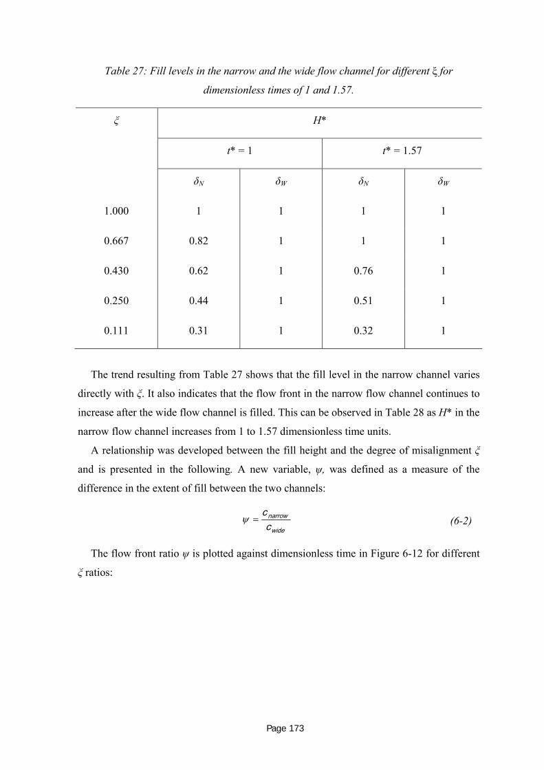
Page 173
Table 27: Fill levels in the narrow and the wide flow channel for different ξ for
dimensionless times of 1 and 1.57.
H*
t* = 1 t* = 1.57
ξ
δN δW δN δW
1.000 1 1 1 1
0.667 0.82 1 1 1
0.430 0.62 1 0.76 1
0.250 0.44 1 0.51 1
0.111 0.31 1 0.32 1
The trend resulting from 744HTable 27 shows that the fill level in the narrow channel varies
directly with ξ. It also indicates that the flow front in the narrow flow channel continues to
increase after the wide flow channel is filled. This can be observed in Table 28 as H* in the
narrow flow channel increases from 1 to 1.57 dimensionless time units.
A relationship was developed between the fill height and the degree of misalignment ξ
and is presented in the following. A new variable, ψ, was defined as a measure of the
difference in the extent of fill between the two channels:
wide
narrow
cc
=ψ (6-2)
The flow front ratio ψ is plotted against dimensionless time in 745HFigure 6-12 for different
ξ ratios:

Page 174
Figure 6-12: Numerically predicted flow front ratio ψ versus t* for different flow channel
width ratios ξ.
We notice that for different flow channel width ratios ξ different constant flow front
ratios ψ were obtained. Note the dimensionless time scale, which is terminated at 0.8 units.
At this time the adhesive begins to flow out of the wider flow channel. The flow front ratio
is independent of the flow front position only while both flow channels are not filled
entirely, which is not true for t*>0.8. In sub-section 746H6.3.2 the causes that lead to the
asymmetrical adhesive distribution for laterally misaligned insertions will be discussed.
There it will be shown that the position of a pressure maximum underneath the insertion
plate causes the adhesive distribution. The pressure maximum position depends on the ξ-
ratio. As long as both the adhesive flow front in the narrow and in the wide flow channel
remain within the flow channels, i.e. do not flow out at the top of the flow channel, the
pressure maximum position remains unchanged. Consequently, the flow front ratio ψ is
independent of the dimensionless time within this range.
In 747HFigure 6-13, the flow front ratio is plotted with respect to the flow channel width
ratio.

Page 175
Figure 6-13: Relationship between the flow front ratio and the flow channel width ratio
derived from the numerical predictions.
Clearly, from an inspection of Fig.6.13, the relationship between flow front ratio and the
flow channel width is linear. If this is fitted by regression one obtains
0728006831 .. −= ξψ . (6-3)
However, this is clearly wrong at a flow channel width ratio of 0, i.e. when the narrow
flow channel width is closed; here, the flow of the adhesive can only be into the wide
channel and consequently the flow front ratio must also be 0. Given the form of the data
and applying this constraint, it would seem that a physically better and more general fit
would be ξ = ψ, i.e. the flow front ratio is always equal to the flow channel width ratio. The
argument below presents a rational basis for such a relationship.
ξψ = (6-3a)
The cause of the adhesive distribution will be shown in sub-Section 6.3.3 to be the
maximum pressure position underneath the insertion plate. This position depends on the
flow channel width ratio, being shifted closer to the narrow flow channel with decreasing
flow channel width ratio. Given that the flow distribution is equal for ξ = 1 and, as stated

Page 176
above, if ξ = 0 ψ must be 0, and finally for all other investigated flow channel width ratios
ξ the approximation ξ = ψ is close, equation (6─3a) is valid for the considered range of
parameters.
Hence, for a given flow channel width ratio ξ the flow front ratio ψ can be derived for
the considered input parameters. The dependence of the relation on the input parameters
was also tested and results will be reported on in the following sub-section.
Then, assuming the adhesive begins to flow out of the wider flow channel, the flow
front in the narrow flow channel can also be derived, and the missing amount of adhesive
in the narrow flow channel can be calculated. This amount can then be added to the initial
adhesive amount so that complete flow channel filling is ensured if equation 748H(6-3a) is
independent of the initial adhesive amount. This is validated in sub-Section 749H6.3.1.4. We
summarised the procedure to ensure entire filling of both flow channels for laterally
misaligned insertions:
a) Measure dimensions of the Pi-slot and insertion plate,
b) derive minimum adhesive volume to theoretically fill flow channels and area
underneath the insertion plate head entirely,
c) include a safety factor of e.g. 1.1,
d) calculate the minimum initial adhesive height in the Pi-slot, 0H , resulting from the
adhesive volume,
e) estimate lateral misalignment which results from the spacer diameter (spacer
diameter should be chosen as perfectly aligned flow channel width minus 10 %, so
0.45 mm for a 0.5 mm flow channel width),
f) calculate the resulting worst case flow channel width ratio ξ,
g) estimate flow front in narrow flow channel when wide flow channel just fills
according to ξψ 11 HHcN == ,
h) calculate H2, which specifies the unfilled narrow flow channel length,
NcHH −= 12 ,
i) and update H0 according to addition of H2 and 0H .
This approach is conservative because as shown in 750HTable 27 the flow front in the narrow
flow channel continues to increase after the adhesive flows out of the wide flow channel.
Hence, a 2nd equation was derived, which would be valid after the adhesive flows out of
the wide flow channel.

Page 177
First, the flow front ratios with respect to dimensionless time for different flow channel
width ratios were considered (751HFigure 6-14). The time period was defined from the point
when the adhesive flows out of the wide flow channel until either the flow front in the
narrow flow channel reaches the top (e.g. for ξ = 0.667 in 752HFigure 6-14) or until the end of
the flow process (all other ξ ratios in 753HFigure 6-14) is reached.
Figure 6-14: Flow front ratios for different flow channel width ratios after the adhesive
has reached the outflow in the wide flow channel.
The flow front ratio decreases linearly with dimensionless time for all misalignments.
The rate of decrease increases with increasing ξ. One dimensionless time to derive a
relation between the flow front ratio ξ and the flow channel width ratio ψ was specified,
which would provide a worst case scenario; this is when the ISF process terminates
because the flow front ratio value ψ is minimum. In the cases considered in Figure 6-14
this time is 1.6. For the ξ =0.667 case, the ψ value chosen was the one when the adhesive
flows out of the narrow flow channel at t*=1.37. The relations are plotted in 754HFigure 6-15:

Page 178
Figure 6-15: Relation between the flow front ratio and flow channel width ratio for a
specifed dimensionless time of t*=1.35.
Again an approximately linear relation was obtained between the flow front ratio ψ and
the flow channel width ratio ξ. The flow front ratio is now referred to as ψ2:
08520916702 .. −= ξψ (6-4)
A second procedure is proposed to estimate the necessary initial adhesive amount to
ensure complete flow channel filling. This procedure will be presented in sub-
Section 755H6.3.1.4 where the effect of initial adhesive amount on adhesive flow was evaluated.
The effect of insertion speed, adhesive viscosity, insertion plate width and insertion plate
head shape is also considered in the following sub-section.
6.3.1.2 Effect of the insertion speed
Absolute Pi-joint dimensions remained unchanged to those presented in the previous
sub-section. The flow channel width ratio was specified as 0.430. For these parameters the
insertion speed was derived for an adhesive viscosity of 70 – 30 weight percent EA 9395 to
EA 9396 and the fill height H* determined with respect to dimensionless time (756HFigure
6-16).

Page 179
Figure 6-16: Predicted fill heights with respect to dimensionless time in the wide and
narrow flow channel (ξ = 0.430) for two different insertion speeds and 70 – 30 weight
percent EA 9395 to EA 9396.
At different insertion speeds (60 and 120 mm/min), small differences can be observed
from the predicted fill heights for different process conditions. Hence, for the range of
input variables considered here the effect of insertion speed on the fill height is negligible.
It is highly likely that the insertion speed does not affect the ξ-ψ-relationship, however
further study is necessary to validate this.
6.3.1.3 Effect of the adhesive viscosity
The input parameters remained the same as in the previous sub-section 757H6.3.1.2. At low
insertion speeds of 60 mm/min, the adhesive viscosity was varied and the fill height H*
was predicted. The effect of the adhesive viscosity on the fill height H* is illustrated in
758HFigure 6-17.
Figure 6-17: Predicted fill heights with respect to dimensionless time in the wide and
narrow flow channel (ξ = 0.430) for two different adhesive viscosities at an insertion speed
of 60 mm/min.

Page 180
The adhesive viscosity scarcely affects the transient fill height. Hence, it was concluded
that most probably the adhesive viscosity does not affect the relationship derived between
the flow channel width ratio and the flow front ratio in the considered range. In general, it
is assumed that this relationship is not affected by the adhesive viscosity. To ensure this
independence, an extension of the adhesive viscosity range simulated is needed.
6.3.1.4 Effect of the initial adhesive amount
Using baseline input variables, the initial adhesive amount applied into the Pi-slot
before starting the bonding process was varied. To evaluate this effect on the adhesive
flow, a flow channel width ratio of 0.430 was considered. This parameter was selected as
the previous simulations had found that the narrow flow channel could not be entirely
filled for an initial adhesive amount of 125 volume-percent. Plots illustrating fill heights in
the narrow channel for four simulations differing in the initial adhesive amount are
presented in 759HFigure 6-18.
Figure 6-18: Fill height as a function of dimensionless time in the narrow channel for a ξ
ratio of 0.430 for different initial adhesive amounts.

Page 181
As expected, fill heights increase with dimensionless time for all considered
simulations. The total flow time until the ISF process terminates varies with the initial
adhesive amount. The initial adhesive fill height H* at t* = 0 is also affected by the initial
adhesive amount. The initial fill height is 0.410 for an initial adhesive amount of
200 volume percent whereas for 125 volume-percent the fill height is 0.25. It can be seen
that the narrow flow channel can be filled for the case where 200 volume percent was
applied (t* = 2.30). For none of the other cases presented here can the top of the flow
channel be reached. An approximately linear increase can be seen initially in the slopes of
the plots, followed by a slightly flatter second increase. This again indicates that the
outflow of the adhesive has occurred in the wider channel, which clearly occurs earlier for
the initially higher filled channels.
Deriving the flow front ratio ψ from the numerical results presented in Figure 6-17 with
equation 760H(6-3), it was found that for this value of ξ the flow front ratios varyied between
0.38 and 0.39 for initial adhesive amounts between 125 and 200 volume percent as long as
both flow channels were not filled entirely.
As indicated in sub-Section 761H6.3.1.1, a second procedure was developed to ensure full
filling of flow channels that can be applied for times after the wide flow channel is filled
with adhesive entirely. This procedure was applied to the results for varying flow channel
widths for a flow channel width ratio of 0.430. The following variables were defined:
− H0, stop was defined as the distance the insertion plate can travel from its initial
position until touching the Pi-slot bottom;
H0H0, totalH0H0, total
Figure 6-19: Definition of H0, total which is used for the second procedure to ensure entire
filling of the narrow flow channel in a misaligned insertion process.

Page 182
− cW0 and cN0 were defined as the flow front positions in the wide and the narrow
flow channel, respectively, when the adhesive flows out of the wider channel, and
cW2 and cN2 were the flow fronts after that time;
− cN2,total was defined as the sum cN0 and cN2, and cN2, missing was defined as the flow
channel height H1 minus the initial adhesive height H0 plus cN2,total
− H0* was the entire distance travelled at that time, and h* was the remaining
possible travel distance before the insertion plate and Pi-slot touch.
Having defined these variables, the procedure was as follows:
1 Assume H0 and calculate H0, stop;
2 calculate cW0 and cN0 with
010 HHcw −= (6-5)
0
0072800683331W
N
cc
)..( =−= ξψ ; (6-6)
3 calculate H0* and h* with
wwNN cc*aH δδ 0002 += (6-7)
*HH*h total, 00 −= ; (6-8)
4 calculate cN2 from
2
22 0852091670
W
N
cc
)..( =−= ξψ (6-9)
wwNN cc*ah δδ 222 += (6-10)
222
12ψδδ
ψNW
N *ahc+
=⇒ ; (6-11)
5 calculate c2,total which results from cN0 and cN2, and add to the initial
adhesive height H0, and subtract from H1, to find out missing flow front in
narrow channel, hence cN2, missing = H1 - H0 + cN0 + cN2;
6 finally, terminate if cN2, missing is less than 0, but add cN2, missing to H0 and start
from 1 if cN2, missing is greater 0.
This procedure was applied for ξ=0.430 when the initial adhesive amount was defined
as 125 volume percent. It was calculated that applying an initial adhesive amount of

Page 183
189 volume percent should result in a complete filling of the narrow flow channel.
Comparing this with 762HFigure 6-18 we notice that complete filling is achieved somewhere
between 175 and 200 initial volume percent, hence the estimation is in line with the
numerical results. Compared with the procedure proposed in sub-Section 763H6.3.1.1, this
approach requires more calculation in determining the minimum required initial adhesive
amount; however, this second procedure is more accurate, being consistent with the
numerical predictions, and hence has the capacity to reduce adhesive wastage.
6.3.1.5 Effect of the total flow channel width
The effect of varying the insertion plate width on the distribution of the adhesive within
the flow channels was also investigated. For this purpose the Pi-slot width was kept
constant (6.0 mm) and the insertion plate width was varied between 4.8 and 5.2 mm. Other
input variables that were kept constant were the insertion speed (60 mm/min), the adhesive
viscosity (70 – 30 volume percent ratio mixture of EA 9395 to EA 9396) and the initial
adhesive amount (125 volume percent).
764HFigure 6-20 presents the fill heights within the narrow channel with respect to
dimensionless time for three different ξ ratios (1.5, 2.3 and 3), each for three different total
flow channel widths (0.8, 1.0, 1.2 mm).

Page 184
a) ξ = 0.667 b) ξ = 0.430
c) ξ = 0.333
Figure 6-20: Effect of the total flow channel width on the fill height versus dimensionless
time for a) ξ = 0.667, b) ξ = 0.430, and c) ξ = 0.333.
The graphs show that the dimensionless adhesive amount at time t*=0 varies slightly for
different δtotal. This is because the initial adhesive amount of 125 volume percent differs for
different absolute dimensions, with the widest total flow channel width of 1.2 having the
highest adhesive amount at t*=0 in all three cases.
Considering a ξ ratio of 0.667 ( 765HFigure 6-20 a)), it appears that there is less resistance to
the flow in those cases where δtotal is smaller. Consequently, the gradient H*/t* is highest
for δtotal = 0.8 mm, indicating the fastest filling out of the three investigated cases. The
slowest filling rate occurs for the widest total channel. This trend can also be observed
when the ξ ratio is decreased. For example, 766HFigure 6-20 b) (ξ ratio 0.430) indicates fastest
filling for the narrowest flow channels, although the flow channels cannot be filled
completely. For the smallest ξ ratio investigated the difference in filling the flow channels
for different total flow channel widths is not as strong as for the lower ξ ratios. From these
results it is concluded that there is little dependence on the filling of the flow channels

Page 185
from the total flow channel width. This can be seen from the different filling gradients. The
effect seems to weaken for higher ξ ratios.
To emphasize the effect of total flow channel width on flow front ratios ψ these are
plotted for the above-presented flow channel width ratios in 767HFigure 6-21.
Figure 6-21: Flow channel width effect on the flow front ratio ψ, resulting from a variation
of the insertion plate width, plotted for three different flow channel width ratios ξ.
768HFigure 6-21 shows that there is little difference in the flow front ratios for the differenct
widths. With increasing flow channel width the flow front ratios appear to decrease
slightly. For example for the highest flow channel width ratio considered (0.667), the flow
front ratio decreases from 0.645 to 0.624 for an increase in total flow channel width from
0.8 to 1.2 mm. This trend weakens for smaller ξ ratios, for example for ξ = 0.333 ψ only
decreases from 0.272 to 0.269.
In summary, it has been shown that there is a dependence between the ξ ratio and the
adhesive distribution during an ISF process. The flow within the narrow channel was
examined for a number of simulations where several input parameters were varied, i.e. the
insertion speed and adhesive viscosity. Both have little effect on the adhesive flow fronts.
Similarly, the initial adhesive fill height also only slightly affected the flow front ratio ψ,

Page 186
Finally, it has been found that the flow front ratio ψ decreases slightly with increasing total
flow channel width δtotal. This effect was stronger for higher flow channel width ratios ξ.
6.3.2 Explanation of asymmetrical adhesive flow
Within this sub-section the causes of an asymmetrical adhesive distribution within
misaligned joints are examined. The sample used for the analysis was the ξ ratio case of
0.430 with an insertion plate width of 5.0 mm and Pi-slot width of 6.0 mm, i.e. a
misalignment of 0.2 mm. The resulting flow channel widths were 0.7 mm and 0.3 mm. The
input parameters were 60 mm/min for the insertion speed and 70-30 weight percent
EA 9395 to EA 9396 adhesive viscosity.
The pressure distributions underneath the insertion plate for a symmetrically aligned
case and ξ = 0.430 are shown in 769HFigure 6-22 at t* = 0.28.
a) b)
Figure 6-22: Static pressure distribution within the flow domain for t*=0.28 for a perfectly
aligned insertion of a) ξ = 1 and a laterally misaligned insertion defined by b) ξ = 0.430.
A pressure maximum exists in the area centred underneath the insertion plate bottom for
the aligned case (770HFigure 6-22 a)). In 771HFigure 6-22 b), the pressure maximum is positioned
closer to the narrow channel. As the particles’ motion would be expected to be away from
the maximum pressure, and in addition given there is only one pressure peak in the flow
domain, the position of the maximum pressure is considered as the main cause for the
distribution of the adhesive.

Page 187
Streamlines within the flow domain of the ξ = 0.430 case for the same time to illustrate
the flow of the adhesive where considered and are illustrated in 772HFigure 6-23.
Figure 6-23: Streamlines implying the flow of the adhesive for a misaligned insertion
defined by ξ = 0.430 at t* = 0.28.
These streamlines indicate that the main flow direction from underneath the insertion
plate is directed towards the wider flow channel. The streamlines are directed away from
the maximum pressure location; as there is only one maximum pressure in the flow
domain, its location is considered as the cause for the distribution of the adhesive.
For the cases studied in sub-Section 773H6.3.1.1 the pressure distributions underneath the
insertion plate were determined at t* = 0.28. The results are displayed in 774HFigure 6-24.
Within 775HFigure 6-24 an x-position of -3 mm represents the left Pi-slot wall position and the
right wall is at 3 mm. For the perfectly aligned case of equal 0.5 mm flow channel width
on both sides the left insertion plate wall is located at -2.5 mm and the right insertion plate
wall is located at +2.5 mm.

Page 188
Figure 6-24: Pressure distribution along the insertion plate bottom for differently
misaligned cases for t*=0.28.
For all cases in 776HFigure 6-24 there is a similar shape to the pressure profile along the x-
axis. The pressure is always higher underneath the insertion plate compared to the pressure
that is in the flow channels, hence next to the insertion plate. As the degree of
misalignment increases the left flow channel width decreases, which is indicated by the
shift of the graph to the left hand side for higher misalignments. The insertion plate width
remains constant for all cases at 5.0 mm.
777HFigure 6-24 shows that the pressure distribution under the insertion plate changes only
slightly with misalignment. For each case a pressure maximum was detected, with its
position depending on the misalignment. For example, in the non-misaligned case this
maximum is located in the middle underneath the insertion plate bottom. It is displaced
towards the narrower flow channel when the insertion plate is misaligned with greater
displacements for greater misalignments (decreasing ξ).
To emphasize the maximum pressure location, the dp/dx gradient along the insertion
bottom plate for the same cases is plotted in 778HFigure 6-25.

Page 189
Figure 6-25: Pressure gradients along the insertion plate bottom for different misaligned
cases for t*=0.28.
For the symmetrically aligned case and misalignments of 0.1 mm (ξ = 0.667) and
0.2 mm (ξ = 0.430) there are three zero dp/dx-position in the middle region underneath the
insertion plate.This area is where the maximum pressures are found for these cases, and as
described above, the particles’ motion was away from these positions. For the other
misaligned cases the position of the maximum pressure is located out of the plotting region
and melds with another pressure peak which is located at the corner of the insertion plate at
the narrow flow channel side. For these cases the adhesive flow is also away from the
pressure maximum location, which results in more adhesive flowing towards the wider
flow channel side.
6.3.3 Effect of different insertion head shapes
The effect of the insertion plate gemetry on the adhesive distribution was investigated to
see whether there is a favourable design that would allow improved filling of the narrow
flow channel if the plate is misaligned. The investigated insertion head shape designs were
those illustrated in 779HFigure 5-24 on page 780H151.

Page 190
Keeping the insertion plate and Pi-slot widths constant, the insertion plate was
misaligned with 0.1 mm. The resulting flow channel width ratio ξ is 0.4/0.6 = 0.667.
Material and process parameters were adhesive viscosity =70 – 30 mix, insertion
speed =60 mm/min and the initial adhesive amount =125 volume percent; all remained
constant for these tests. The fill height with respect to the time is plotted for the four
different insertion head shapes in 781HFigure 6-26.
Figure 6-26: Transient fill height in the wide (W) and narrow (N) flow channels for
different insertion head shapes.
As expected, the wider flow channels fill more quickly than the narrow ones but there is
some difference in the rate at which the wider flow channel fills with head shape.
Interestingly the rectangular design (shape 4) fills first, then the rounded head (shape 3)
and finally the two tapered heads, with design 1 filling last. This general trend results from
the initial adhesive flow; for the rectangular head the adhesive flows directly into the flow
channels. However, for the rounded and more so for the tapered heads, the adhesive fills
the tapered or rounded areas of the insertion plate head between the insertion head and the
Pi-slot walls first, and only then begins to fill the flow channels. Hence the filling is slower
simply due to the law of mass conservation and due to larger areas for the rounded and
tapered heads to be filled compared to the rectangular head.

Page 191
In all but one case (the rounded shape) all the narrow flow channels filled. For the
rounded case the narrow channel did not fill due to the having an insufficient initial
adhesive amount. As mentioned previously, when applying 125 volume percent the
absolute amount of adhesive flowing out at the top of the flow channels for the rounded
case is considerably smaller than the amount in, for example, the rectangular case.
Applying more initial adhesive amount than 125 volume percent would be needed when
the insertion plate head is rounded to ensure complete filling. In general, the quickest
filling is achieved with the rectangular head due to the reason that the adhesive fills the
flow channels directly, which is not the case for all other investigated head shapes, as
described in the previous paragraph.
To evaluate the effect of insertion head shapes on the adhesive flow in both flow
channels we derived flow front ratios for the investigated ξ ratio with respect to insertion
head shape (782HFigure 6-27):
Figure 6-27: Flow front ratios for different head shapes for a misaligned insertion defined
by ξ =0.667.
More equal adhesive distributions are predicted for both tapered insertion head shapes,
which referred to as shape 1, which has a longer taper, and shape 2, which is tapered

Page 192
shorter. The more equal filling with tapered insertion heads is due to the initial adhesive
distribution before the adhesive flows into that flow channel’s area which remains constant
in width. The equal filling of the area between the tapered region of the insertion head and
the Pi-slot walls can be explained as follows: the ratio of the flow channel widths in this
area is close to 1 because the total flow channel width is large. In the initial stages of the
process the local flow channel width ratio for the longer tapered shape (shape 1) would be
ξlocal = 2.65/2.85 = 0.93. The adhesive flow would behave as in an almost perfectly aligned
case. Once the adhesive is displaced further and reaches the region where the flow channel
widths are different, the distribution becomes asymmetrical, as can be observed from
783HFigure 6-26 for the longer tapered shape (shape 1) after about 2.5 s.
To sum up, adhesive distribution was affected by the insertion head shape, with the
most symmetric adhesive flow observed for tapered heads. The rectangular insertion plate
head which was modelled in most of the presented simulations throughout this research
showed the least equal adhesive distribution. Hence, simulating the rectangular shape can
be considered as a worst case scenario.
6.4 Mitigating the Effects of Lateral Misalignment
In this section, the number of spacers needed to control alignment between the insertion
plate and the Pi-slot, and hence flow channel width, is discussed. The results of a
calculation of the bending forces on the insertion plate through applied spacers are also
discussed.
6.4.1 Use of spacers
If the insertion plate and the Pi-slot were perfectly straight, did not vary in thickness,
and remained so during the ISF only two spacers, one positioned at each end of the joint,
would be needed to allow perfect alignment between the two components. However, in
Section 784H6.1 it was shown that manufacturing tolerances and process-induced distortion are
very common and will affect the flow channel widths. To ensure a pre-defined required
flow channel width ratio, more spacers need to be applied over the Pi-joint length to force
the insertion plate to bend back within the Pi-slot. The number of required spacers was
estimated and results of the necessary number of spacers for a certain set-up are presented
within this sub-section. In sub-Section 785H6.4.2, the force necessary to bend the insertion plate
is calculated.

Page 193
The minimum distance between two spacers required was derived by applying the
following assumptions (Liu, 2009):
− The insertion plate is rectangular with dimensions as specified in 786HFigure 6-28 being
300 mm, 5 mm and 1320 mm for the height H, width W and length L;
x
y
z
L
WHx
y
z
L
WH
Figure 6-28: Variables defining the dimensions of the insertion plate.
− There is no penetration of spacer into the composites (i.e. the spacers restrain the
insertion plate);
− the Pi-slot is perfectly straight and does not deform during ISF;
− bending of the insertion plate in the z-direction is assumed to form a circular
arc (MoJo, 2007);
− as illustrated in 787HFigure 6-29 after the spacers are applied the insertion plate region
between the two spacers also bends as a circular arc;
− the deflection limit is set to 10% of the total flow channel width of a standard Pi-
joint, hence 0.1 mm.

Page 194
R
Δ
R
δLspacer
R
Δ
R
Δ
R
δLspacer
Figure 6-29: Circularly bended insertion plate before and after restrained by spacers.
To calculate the radius of bending, geometrical relations according to 788HFigure 6-30 and
provided in equation 789H(6-12) were used:
ΔΔ
22 22 )/L(R +
= (6-12)
R
Δ = 1 mm
δ
Lspacer
L = 1320 mm
R
Δ = 1 mm
δ
Lspacer
L = 1320 mm
Figure 6-30: Geometrical relations for estimating the number of spacers (not to scale).
The radius R was calculated to 217.8 m if L and Δ were substituted into equation 790H(6-12).
Rearranging and solving for Lspacer according to the geometrical relations from 791HFigure 6-30,
the distance between two spacers can be calculated as:
222 δδ −= RLspacer (6-13)
For the specified values of L (1320 mm) and deflections limits for δ (0.1 mm) the
calculated distance was 417.4 mm. Hence five spacers would be needed with an actual
distance between each spacer of 330 mm.

Page 195
6.4.2 Bending forces on insertion plate due to spacers
To calculate the bending forces acting on the insertion plate due to applied spacers, we
assumed the insertion plate to behave as a simply supported beam, as shown in 792HFigure 6-31
for the case considered in sub-Section 793H6.4.1:
FFFF
Figure 6-31: A simply supported beam model applied for the calculation of the bending
force that acts at the insertion plate due to spacers.
The middle spacer was substituted with a force F. Before calculating F, the actual
distance between spacers was derived to be 1320 mm/5 = 330 mm and from equation
794H(6-13) the actual deflection to be δ = 0.06 mm. Now, applying the classic beam
theory (efunda, 2009), the force to cause a deflection of δ can be calculated as:
( ) ( )336
2
48
spacerspacer L
EI
L
EIF δδ −=−= (6-14)
E specifies the Young’s modulus (in-plane) of the insertion plate, which is taken as
50 GPa, and which was provided for the insertion plate as a good approximation although
considered as isotropic, which indeed is not the case for a composite. I is the moment of
inertia of the beam section and Lspacer was taken as 330 mm. I can be calculated as
433
312512
530012
mm*HWI === . (6-15)
Substituting all variables into equation 795H(6-14) results in a force of 1.57 N.
6.5 Summary
Misalignments that may occur during ISF are angular or lateral, with the latter found to
be the most critical one for the adhesive distribution as it affects the flow channel widths.
Lateral misalignment and a variation of flow channel widths can be caused by
manufacturing tolerances, composite spring-in effects and can be induced through the
insertion process.

Page 196
It was found that the adhesive flow strongly depends on the flow channel width ratio,
showing a linear relation between the flow front ratio and the flow channel width ratio of
the narrow and wide flow channel. This relation is not affected by the insertion speed, the
adhesive viscosity nor the initial adhesive amount for the ranges considered, and scarcely
depends on the total flow channel width. Following the research done here, two procedures
were proposed to ensure entire filling of the narrow flow channel.
The insertion plate head shape was found to affect the relation between the flow front
ratio and the flow channel width ratio. The rectangular shape is found to be the one that
results in the poorest filling of the channels in terms of equal adhesive distribution, while
the most equal filling of the flow channels is found for the longer tapered insertion head
design.
Finally, mitigation of lateral misalignment effects can be achieved through the use of
spacers. The distance between the spacers depends on the required tolerancing, using the
case studied here as an example, an approach was developed for determining spacer
placement to meet tolerancing required. The consequential bending forces acting on the
insertion plate due to the spacers were also calculated.

Page 197
7 Extensions of the Numerical Model for Insertion Squeeze Flow
This chapter contains four sections. First, insertion squeeze flow (ISF) at constant
insertion force is considered. Following this a variation of the ISF process is examined,
which considers the pre-application of adhesive onto the Pi-slot walls. Third, the effect of
the fluid structure interaction (FSI) on the adhesive flow during ISF at constant speed is
analysed, i.e., to examine the effect of slot distortion during the process due to the high
pressures on the walls. Finally, the two-dimensional (2D) numerical model presented in
previous chapters is extended into a three-dimensional (3D) model to consider possible 3D
flow variations and the effect of spanwise misalignment. The chapter is summarised with
concluding remarks.
7.1 Insertion Squeeze Flow at Constant Insertion Force
7.1.1 Introduction
An ISF process can be conducted using controlled insertion, with either constant speed
or constant force. In a constant force controlled insertion mode, as implied, the insertion
plate movement is achieved through the application of a constant force upon the insertion
plate. In practice, a constant force insertion can be achieved through the use of pneumatic
pressure cylinders.
Considering basic physical relations describing the problem, drag forces acting on the
insertion plate resist the motion of the insertion plate. As mentioned earlier, these drag
forces can be subdivided into two components: the shear force on the sidewalls and the
pressure force on the bottom wall of the insertion plate. In the constant speed insertion
analysis, these force components represent the retarding force, that frequently has been
referred to as the insertion force. For constant speed insertions, this force was observed to
increase with displacement of the insertion plate. Hence, it would be expected that during a
constant force insertion, the motion of the insertion plate would slow the further it
descends into the adhesive because of the increasing resisting pressure and shear.
Within Section 796H7.1 a numerical model is developed which simulates an ISF process
conducted at constant force insertion. The variables recorded include the insertion plate
speed, acting forces and pressures, as well as the adhesive flow in the flow channels. For

Page 198
validation purposes, we considered if the above described physical actions can actually be
observed. A comparison is made between the constant force and the constant speed
variants with reference to the insertion speed versus displacement behaviour.
7.1.2 Numerical Method
Within Fluent the velocity components can be set to apply a prescribed motion to a
specified boundary. A force cannot directly be specified to act at a boundary. The time-
dependent velocity of a moving boundary that results from an applied force has to be
calculated as part of the time-stepping procedure.
The approach applied to derive the moving boundary velocity is based on a force
balance on the moving object, which in this case is the insertion plate. 797HFigure 7-1 illustrates
the problem set-up again at the left. On the right, parameters are introduced which have to
be taken into consideration for a force balance on a moving insertion plate.
2b
2a
H0
H1
c
2b2b
2a2a
H0
H1
c FτW
Fp
m
a, Fc
FτW
Fp
mm
a, Fca, Fc
2b
2a
H0
H1
c
2b2b
2a2a
H0
H1
c FτW
Fp
m
a, Fc
FτW
Fp
mm
a, Fca, Fc
Figure 7-1: Schematic problem set-up and definition of parameters for the force balance.
On the right hand side of 798HFigure 7-1, a represents the acceleration of the insertion plate,
Fc is the constant force applied to the insertion plate, Fp is the pressure force and FτW is the

Page 199
wall shear force. It is assumed that the insertion is strictly in the verical direction so that
only the verical force balance is of interest. The mass of the insertion plate is represented
by the symbol m.
Applying a force balance on the insertion plate in the vertical direction gives:
cWp FFFma −+=⋅ τ (7-1)
Writing the acceleration a in terms of the rate of change of the velocity (dv/dt) and
rearranging gives an expression for the change in insertion plate velocity over a timestep:
[ ]cWp FFFmdtdv −+⋅= τ (7-2)
Thus the velocity can be incremented each timestep to maintain the constant insertion
force. In this expression, Fc and m are constant, while Fp, FτW (and possibly dt) are time-
dependent variables, hence an iterative update is required. This can be accomplished by
using a user-defined function (UDF) within the Fluent software to return the velocity given
the force components.
The Fluent UDF manual states that “A user-defined function, or UDF, is a function […]
that can be dynamically loaded with the Fluent solver to enhance the standard features of
the code”, ll. 16-17, p. 1-1,(Fluent, 2005a). It is written by the user in the C programming
language and makes use of predefined macros that are provided by Fluent and defined in
header files (Fluent, 2005a). The Fluent UDF user guide (Fluent, 2005c) gives details on
the construction of UDFs.
In the case considered here, a constant-force moving-boundary UDF was programmed
and applied to simulate a constant force ISF process. The programmed UDF file is
provided in Appendix A.
The following block diagram is provided to show the interaction of the UDF and the
flow solver of Fluent:

Page 200
UDF:
balancing acting forces, determining dv,
adjusting v += dv
FLUENT:
moving insertion plate with v,predicting resisting forces
Providing resistingforces to UDF
Providing insertion velocity to FLUENT
Figure 7-2: Block diagram showing the interaction between the constant force UDF and
the Fluent software.
Based on the forces acting, within the UDF the force balance calculation is conducted
according to equation 799H(7-2). The computed velocity change is added to the velocity at the
previous time step (n-1), which is passed to the flow solver to define the plate boundary
velocity. Fluent then applies the newly determined velocity for timestep n to the moving
boundary and advances to the next timestep (n+1) when iteration terminates if convergence
criteria of the continuity and momentum equations are reached. The boundary moves
according to this velocity. Pressure and shear forces along the insertion plate walls are
calculated and provided to the UDF. Using these newly obtained forces, the rate of velocity
change for the next time step (n+1) is calculated within the UDF, then the velocity is
updated and provided to Fluent again. This procedure is conducted every time step.
7.1.3 Results and discussion
The results presented in this section were obtained from the numerical model for
constant force insertion for the set of the baseline parameters unless otherwise stated. The
baseline parameters were a constant insertion force of 3000 N/m, an adhesive viscosity for

Page 201
a 70-30 weight percent ratio EA 9395 to EA 9396 implemented according to the five
parameter rational model, and standard dimensions, which were 5.00 mm insertion plate
width, 6.00 mm Pi-slot width and 35.5 mm Pi-slot height. The Pi-slot bottom inner radius
was 3 mm. The selected value for the standard constant insertion force was set from an
estimation of the imposed pneumatic cylinder pressure on the insertion plate during the
practical insertion process (Scholler, 2007). The widths of the gaps between the insertion
plate and the Pi-slot wall (flow channel widths) were 0.5 mm for the aligned case. The
volume of adhesive was specified as 125% of the volume required to fill the flow channels
completely when the insertion plate reaches its final position. The shape of the insertion
plate head was rectangular.
800HFigure 7-3 shows a plot of the insertion plate speed as a function of the displacement of
the insertion plate during the ISF process.
Figure 7-3: Insertion plate velocity as a function of the insertion plate position for a
constant force of 3000 N/m. The crosses show results from constant speed tests when the
insertion force is equal to 3000 N/m.

Page 202
The y-axis shows the speed of the insertion plate in the vertical direction that results
from the constant force induced motion. This speed is plotted against the insertion plate
position.
The solid line shows the results for the insertion plate speed directly obtained from a
simulation at constant applied force. The crosses indicate results from constant speed
insertion studies at 60, 40, 30, 20, 10 and 5 mm/s. These points correspond to when the
insertion force is 3000 N/m. They were determined from insertion force versus insertion
plate displacement graphs for the constant speed cases. An example is provided in 801HFigure
7-4 below showing the behaviour for an insertion speed of 30 mm/s.
Figure 7-4: Insertion force versus insertion plate position for an insertion speed of
30 mm/s.
In the magnified inset within 802HFigure 7-4 an insertion force of 3000 N/m can be seen to
correspond to a displacement of 0.57 mm. This displacement matches well with the value
for constant force insertion (also 0.57 mm). When comparing results from the constant
force insertion and constant speed insertion tests it is clear that that the values agree very
well. Further constant force-constant speed comparisons not presented here also show the
same tight match. Hence it was concluded that it is possible to determine the insertion plate

Page 203
speed versus position behaviour indirectly from several constant speed insertion
simulations.
In 803HFigure 7-5 a plot is illustrated of insertion plate speed versus dimensionless time t*
for an insertion force at 3000 N/m:
Figure 7-5: Insertion plate speed plotted against dimensionless time for a constant force
insertion at 3000 N/m.
The time was non-dimensionalised by dividing the process time by the time period for
the adhesive to reach the top of the flow channels. The insertion speed increases
significantly in the initial stages of the process (until t* = 0.00125) before decelerating
afterwards. The insertion speed appears to reach an asymptotic value from a dimensionless
time of about 1 onwards.
The behaviour of the insertion speed versus time reflects what would be expected
during insertion under a constant force: to begin with, the plate speed would increase as the
plate accerlerates until drag increases to a value that is higher than the imposed constant
force. Thus subsequently the plate will decelerate, leading to a slowing of the motion.
The initial insertion plate speed increase can be explained by considering equation 804H(7-2)
and 805HFigure 7-6. In 806HFigure 7-6 the drag force on the insertion plate, i.e. the pressure force at

Page 204
the insertion plate bottom and the shear forces along the insertion plate side walls, is
plotted against dimensionless time.
Figure 7-6: Drag force on the insertion plate with respect to dimensionless time shown by
the solid line. The maximum pressure acting at the Pi-slot walls (dotted line) with respect
to dimensionless time is also shown.
The drag force increases initially (hardly seen in the figure), reaches its peak before
decreasing to a magnitude of slightly in excess of 3000 N/m after about t* = 0.05. The
smaller the drag force over the beginning stage of the process, the larger the resultant
downward force and hence the larger the (negative) acceleration. Hence, as long as the
constant applied force is higher than the drag force the insertion plate speed will
increase (t*<0.00125).
The speed reaches its peak at the moment when the drag force values become greater
than the applied force. After this time the acceleration becomes positive, leading to a
positive dv value and thus to a decrease in the insertion speed (t*>0.00125). For this case,
these events are summarised.

Page 205
[ ]cWp FFFmdtdv −+⋅= τ
cWpdrag FFFF:.*t <+=<≤ τ0012500
0<⇒ dv
11 +− >⇒+= nnnn vvdvvv
cdrag FF:.*t >> 001250
10 −<⇒>⇒ nn vvdv
(7−2)
(7-3)
After reaching a peak, the drag force plotted in 807HFigure 7-6 decreases slowly until it
reaches a similar, but slightly larger, value to the applied constant force. This is reflected in
the continuing deceleration of the insertion plate. The slowing continues reasonably
smoothly until a non-dimensional time of approximately one. At that time the adhesive
reaches the top of the Pi-slot and starts to be extruded out the ends. Hence after this time, it
could be expected that the configuration contributing to the drag, i.e., the adhesive in the
filled gaps applying a shear force to the plate and the pressure at the plate end, does not
change at the same rate. Thus it could be expected that the insertion velocity would
maintain an almost constant value beyond this time. The observed insertion speed variation
with displacement, or time, supports this explanation. Note that there is some variation of
the drag from the constant applied force especially at larger times. It is unclear whether this
is a resolution/convergence issue or a result of nonlinear flow effects associated with the
adhesive flowing out into the open domain or secondary flows at the bottom of the slot.
The pressure acting along the Pi-slot walls is now considered in view of the fact that it
can potentially cause distortion of the slot. Recall that for the constant speed simulations, a
relationship could be established between the insertion force and the pressure on the Pi-slot
walls. For the constant force insertion results here, it is again noticed that there might be a
relationship between these two parameters. Therefore in 808HFigure 7-6 the maximum pressure
acting at the side walls of the Pi-slots is plotted with respect to dimensionless time, shown
by the dotted line. Also, from the constant insertion speed simulation results, it was shown
that the local pressure maximum was always found at the root of the Pi-slot wall (809HFigure
5─17, page 810H138).

Page 206
Considering the pressure graph presented in 811HFigure 7-6, it is noticed that the pressure
increases significantly at the very beginning, then decreases slightly before becoming
constant. A similar trend was detected for the transient drag forces acting on the insertion
plate; hence, it was supposed that a connection between the (plate) force and the (Pi-slot)
pressure exists.
After the initial, sharp increase, followed by a less severe decrease, the pressure levels
out at a magnitude of about 555 kPa. Dividing the drag force of approximately 3000 N/m
by the pressure acting as was previously done for the constant speed simulations in 812HTable
24, page 813H141, the value of F [N/m] / p [kPa] = 5.405 [103m] is obtained. This is within
0.2 % to the force-pressure ratio derived for the constant insertion speed simulations (see
sub-Section 814H5.3.3).
An important parameter for ISF processes conducted at constant force is the process
time. Several simulations were set up with varying constant force values and their effect on
the process time was studied. The simulations used the baseline parameters specified
earlier and the constant applied force levels set to 400 N/m and 2000 N/m in addition to the
already presented case of 3000 N/m. A ‘stop’-position was defined at which the process
time is compared for different values of the applied force. The chosen ‘stop’-position
corresponds to after the insertion plate has travelled 8 mm from its starting positition; the
closest distance between the insertion plate head and the Pi-slot bottom is then 1 mm. The
y-displacement of the insertion plate with respect to flow time is presented in 815HFigure 7-7:
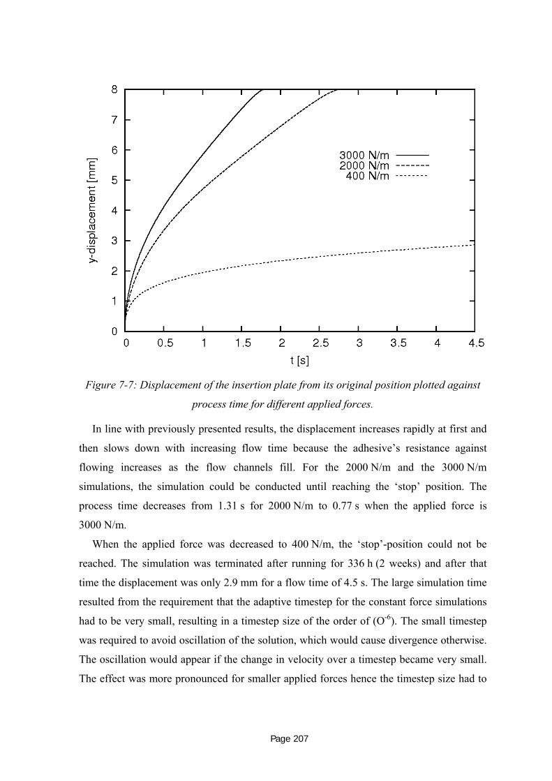
Page 207
Figure 7-7: Displacement of the insertion plate from its original position plotted against
process time for different applied forces.
In line with previously presented results, the displacement increases rapidly at first and
then slows down with increasing flow time because the adhesive’s resistance against
flowing increases as the flow channels fill. For the 2000 N/m and the 3000 N/m
simulations, the simulation could be conducted until reaching the ‘stop’ position. The
process time decreases from 1.31 s for 2000 N/m to 0.77 s when the applied force is
3000 N/m.
When the applied force was decreased to 400 N/m, the ‘stop’-position could not be
reached. The simulation was terminated after running for 336 h (2 weeks) and after that
time the displacement was only 2.9 mm for a flow time of 4.5 s. The large simulation time
resulted from the requirement that the adaptive timestep for the constant force simulations
had to be very small, resulting in a timestep size of the order of (O-6). The small timestep
was required to avoid oscillation of the solution, which would cause divergence otherwise.
The oscillation would appear if the change in velocity over a timestep became very small.
The effect was more pronounced for smaller applied forces hence the timestep size had to

Page 208
be decreased compared with the timestep size specified for the higher force
simulations (2000 N/m, 3000 N/m).
Finally, the effect of a misalignment during plate insertion on the adhesive distribution
is considered. The dimensions of the insertion plate and the Pi-slot remained the same but
the insertion plate was displaced laterally by a value of 0.1 mm. Resulting flow channel
widths for this misaligned case were therefore 0.6 and 0.4 mm for the wide and the narrow
channel. This corresponds to a dimensionless flow channel width ratio ξ = 0.667.
816HFigure 7-8 illustrates the behaviour of the fill height H* versus non-dimensionalised
time.
Figure 7-8: Adhesive flow comparison between a misaligned and a perfectly aligned
constant force ISF process.
The time scale used to non-dimensionalise was the time for the complete filling of both
flow channels for the aligned case. As indicated in 817HFigure 7-8 filling of both flow channels
for a misaligned insertion with a flow channel width ratio of 0.667 is possible. The wider
flow channel fills more quickly; the narrower flow channel is filled after a dimensionless
time of about 1.55.

Page 209
These observations tally with those for constant insertion speed insertions. Agreement
between the simulations with ξ = 0.667 is obtained, in the sense that both flow channels fill
and, of course, that the wider flow channel fills first.
Next, the positions of the flow fronts in the channels were considered by examining the
height ratio of the narrow and wide channel, referred to as ψ. This ratio is plotted against
time in 818HFigure 7-9.
Figure 7-9: Flow front ratio as a function of dimensionless time (ξ=0.667).
Except at the very beginning, the graph shows that the flow front ratio is independent of
time for the considered case of ξ = 0.667, at least up to a dimensionless time of t*=0.6.
This time corresponds to the period before the adhesive starts to flow out of the wider
channel. The ratio remains constant with a value of 0.638.
Recalling the results for the constant speed insertion again, especially considering
819HFigure 6-12 on page 820H174, it can be seen that for ξ = 0.667 the values obtained from the
constant speed insertion and the values from the constant force insertion are very close to
each other. This result indicates that 821HFigure 6-12 can be applied for constant force
insertions as well. To support this suggestion, an explanation is provided why the constant

Page 210
insertion speed and the constant insertion force insertions provide similar relationships
between the output parameters.
The Reynolds numbers for both constant speed and constant force insertion were
considered. For a constant speed insertion, the Reynolds number is in the order of 10-4,
calculated with the following values:
− Density ρ = 103 kg/m3,
− Flow velocity v = 10-2 m/s, derived from insertion speed of 60 mm/min,
− Length scale L = 10-3 m, derived from the flow channel width,
− Adhesive viscosity η = 10 kg/(ms), derived from viscosity versus shear rate graphs
at high shear rates which correspond to the flow velocity;
− All applied values are conservative values within a reasonable range in a sense to
derive a Re number as high as possible.
For a constant force insertion, the Reynolds number is in the order of 10-2, calculated
with the following values:
− Density ρ = 103 kg/m3,
− Flow velocity v = 101 m/s, derived from a maximum insertion speed at a constant
force insertion with 3000 N/m,
− Length scale L = 10-3 m, derived from the flow channel width,
− Adhesive viscosity η = 10 kg/(ms), derived from viscosity versus shear rate graphs
at high shear rates which correspond to the flow velocity;
− All applied values are conservative values within a reasonable range in a sense to
derive a Re number as high as possible.
Hence, the Reynolds numbers for both insertion types are clearly considerably less than
unity, constituting a low Reynolds number flow. This flow typically is governed by a
balance between pressure and viscous forces with inertia effects being negligibly
small (Munson, 2006). For immersed body flows such as the one considered here, the drag
force D consists of two parts; the friction drag due to wall shear stresses and the pressure
or form drag due to pressure forces (Munson, 2006). Furthermore, the drag coefficient cD,
defined as D/(1/2 ρv2A), becomes inversely proportional to the Reynolds number. The
relation between the Reynolds number and the acting drag for the provided information is
considered:

Page 211
AvDcD
2
2
ρ=
Wpdrag FFFD τ+==
constantdependentshapebodyabeingC1;Reif <= ;ReCcD
2
ReC
AvDcD
2
2
2 ==ρ
LAvC
Lv
AvC
Re
AvCFFD Wp
η
ηρ
ρρτ ===+= 2
22
222
(3−35)
(7-4)
(7-5)
It is clear from equation (7-5) that the drag is a function of the flow velocity. In
addition, the pressure varies linearly along the flow channel. This is true for both the
constant speed and the constant force cases, hence there is a correlation between them and
results obtained for one are valid for the other insertion technique.
In conclusion, it was shown that for cases such that Re < 1, the different methods of
insertion (constant speed or constant force) provide equivalent results. This means that for
the considered range of input parameters presented within this research, relationships
established from the constant speed insertion can be applied to constant force insertions.
7.2 Insertion Squeeze Flow with Adhesive Pre-Application
One variation of the ISF process might include pre-applying a thin layer of adhesive on
the insertion plate side walls before conducting the ISF process. A favourable adhesive
flow could be expected in practice as the adhesive would flow over a smoother surface. To
generate this layer adhesive would be applied on the insertion plate walls and excessive
material would be wiped off using a spatula or some similar device. Remaining adhesive
would fill valleys in the composite surface that result from the manufacturing process due
to the use of peel-plies.
When numerically setting up this modified ISF process, the layer of cells adjacent to the
insertion plate was patched with adhesive. Two cases were studied: one where the same

Page 212
adhesive was applied for the layer and into the Pi-slot bottom and a second where the
adhesives differed from each other. The two adhesives were of different viscosity
according to adhesive mixtures that represent the highest and lowest possible viscosities.
An analysis was undertaken to determine in which way the pre-applied adhesive affected
the adhesive flow within the flow channels.
The mesh used for this analysis differed slightly from the standard mesh used for the
previously presented results in the way that more vertical cell layers within the flow
channels were used. Furthermore, the cell layers became finer the closer they were to the
insertion plate wall.
The characteristic flow dimensions were held constant according to the previously
presented results for aligned studies. In terms of input parameters, the insertion speed was
specified as 60 mm/min. The shear viscosity was selected according to adhesive mixtures
between EA 9395 and EA 9396 of 100 – 0 and 70 – 30 weight percent. For the case where
the same adhesive was pre-applied along the insertion plate walls and within the Pi-slot
bottom, the lower viscous mixture was modelled. For the case that involved a three-phase
analysis – when the adhesive on the insertion plate walls differed from the adhesive placed
in the bottom of the Pi-slot – a mixture of 100 – 0 was applied into the Pi-slot and the
lower viscous adhesive was patched onto adjacent layers next to the insertion plate walls.
In Fluent, it was not possible to patch two different UDF material models to regions within
the flow domain. Consequently, the five-parameter rational model could not be
implemented for the three phase flow analysis. The adhesive shear viscosity was defined
according to the Power law. To ensure comparability, the adhesive was also implemented
as a Power law fluid for the two-phase flow simulation.
To illustrate the adhesive pre-application the initial adhesive distribution is shown in
825HFigure 7-10.

Page 213
Figure 7-10: Initial adhesive distribution including pre-applied adhesive on the insertion
plate side walls. Blue shows the initial location of the adhesive.
The red colour represents air and the blue colour represents adhesive. The adhesive that
is pre-applied on the side walls can be, as mentioned earlier, either the same or a different
material.
The output obtained from this analysis provides information about the filling
characteristics of the flow channels. The filling resulting from a standard ISF process was
compared to that from an adhesive pre-applied ISF process. The results are presented in
826HFigure 7-11 as the fill height versus dimensionless time. The fill height H* was defined
previously in equation 827H(6-1) as the the flow front c plus the initial adhesive height H0
divided by the total flow channel height H1.,
1HHcH 0+
=* . (6-1)

Page 214
Figure 7-11: Comparison of fill heights for a pre-applied and a standard ISF bonding
process as a function of dimensionless time. The pre-applied variant was conducted with
two and with three phases, which are presented by the dotted lines.
There is clearly little difference between the two- and three-phase flow pre-applied
cases. The pre-application cases generally fills more quickly due to the adhesive already
within the flow channels. However, using this procedure would add another labour-
intensive step to the ISF process and in turn increase the total process time. A further
consideration would appear to be from oxidization of a micro-layer of the pre-applied
adhesive. There is evidence that joint quality would be affected due to the reduction of
bonding strength from oxidization (Petrie, 2004).
7.3 Insertion Squeeze Flow including Fluid-Structure Interaction
7.3.1 Introduction
For the numerical results presented so far, the Pi-slot wall boundaries are assumed to be
rigid. However, in practice the Pi-slot walls may deflect if the pressure acting on them is
large enough, increasing the width of the flow channels. Consequently, the flow of the

Page 215
adhesive would be affected, and the pressure resulting from the adhesive flow would
change as well. This fluid-structure interaction will be investigated further in this section.
In sub-Section 828H7.3.2, the methodology and problem set-up for the fluid-structure
interaction (FSI) is introduced. Sub-Section 829H7.3.3 deals with results obtained from
numerical simulations which take the FSI into consideration, investigating the effect of
input variables such as Pi-slot wall stiffness and adhesive viscosity on output variables
such as the deflection of the Pi-slot walls and the adhesive flow within the flow channels.
7.3.2 Numerical method
From the results for constant speed insertions, a pressure distribution along the Pi-slot
walls could be determined, for example, as presented in 830HFigure 5-16 on page 831H138. The
pressure maximum was found at the root of the Pi-slot and decreased linearly within the
flow channel dropping to zero gauge pressure at the adhesive flow front. To derive a wall
deflection equation, the pressure is assumed to decrease linearly from the root to the flow
front position. In fact, in the area underneath the insertion plate head, the pressure is
uniform along the Pi-slot wall. This was observed within 832HFigure 5-16 where the pressure
remained constant between a Pi-slot position of 0 mm and 5 mm. It was assumed that the
linear pressure distribution has a minor effect on the results due to two reasons: first, the
distance between the insertion head plate and Pi-slot bottom decreases with respect to time,
indeed, approaching an entirely triangular distribution. Second, in the very beginning,
when the greatest differences exist between the assumed and actual pressure distribution,
the pressure is comparably small. The pressure increases with time, as can be observed in
833HFigure 5-17, page 834H139, and hence is expected to cause a larger distortion towards the end of
the insertion process. By that time, the area of uniformly distributed pressure becomes
even smaller and the pressure distribution is nearly linearly distributed along the Pi-slot,
with a maximum at the root and a minimum at the flow front. 835HFigure 7-12 illustrates the
actual and assumed pressure distribution:

Page 216
Assumed pressure
distribution px(y)
L
H1
y
Pi-slot
Adhesive
flow front
Actual pressure
distribution px(y)
y
x
Assumed pressure
distribution px(y)
L
H1
y
Assumed pressure
distribution px(y)
L
H1
y
Pi-slot
Adhesive
flow front
Actual pressure
distribution px(y)
y
x
Pi-slot
Adhesive
flow front
Actual pressure
distribution px(y)
y
x
y
x
Figure 7-12: Schematic of the actual and assumed pressure distribution along the Pi-slot
wall. This pressure results from the adhesive flow which is also shown in the figure for one
examplary time.
For the assumed and the actual pressure distribution, the error was calculated for
analytical solutions when the adhesive reaches the top of the flow channel. This error is in
the order of
%lH
H%
lHHH
e 100110011
131
41
41
⎟⎟⎠
⎞⎜⎜⎝
⎛−
−=⎟⎟⎠
⎞⎜⎜⎝
⎛
−−= . (7-6)
Given the values for the Pi-slot height H1 = 35.5 mm and the remaining distance
between the insertion plate head and the Pi-slot bottom l = 0.65 mm, the error e = 1.87%.
Given that the error is only very small and conservative, meaning that the distortion
resulting from the actual pressure distribution would be smaller, it was decided that the
assumed pressure distribution is justified to be used for the simulations.
To derive a beam deflection equation for the Pi-slot wall distortion, the Euler Bernoulli
beam equation was applied, modelling the Pi-slot wall as a cantilever beam.
⎟⎠⎞
⎜⎝⎛ −= 104
14
Lyq
dywd
EI for 0 ≤ y ≤L (7-7)
042
4
=dy
wdEI for L ≤ y ≤H1 (7-8)

Page 217
Within equations 836H(7-7) and 837H(7-8), E is the stiffness of the composite, I is the second
moment of area, w is the deflection in the y-direction, q0 is the loading per unit length and
L is the position of the adhesive flow front.
Based on these equations, a function is derived for the deflection of the cantilever
beam (Pi-slot wall):
( )32234531 10105
10LyLyLyy
ELtp
)y(w max −+−= for 0 ≤ y ≤L (7-9)
( )342 5
10yLL
Etp
)y(w max −= for L ≤ y ≤H1 (7-10)
Within equations 838H(7-9) and 839H(7-10), the load per length q0 was substituted by the
maximum pressure pmax multiplied with the length l of the Pi-slot in the z-direction. The
second moment of area I was substituted by 1/12*l*t3, with t being the thickness of the Pi-
slot wall. The deflection is illustrated schematically in 840HFigure 7-13:
x
y
Pi-slot
Adhesive
flow front
Assumed pressure
distribution py(x)
L
H1
w1(y)
w2(y)
L
x
y
Pi-slot
Adhesive
flow front
Assumed pressure
distribution py(x)
L
H1
x
y
x
y
Pi-slot
Adhesive
flow front
Assumed pressure
distribution py(x)
L
H1
w1(y)
w2(y)
L w1(y)
w2(y)
L
Figure 7-13: Illustrated simplification of Pi-slot wall as a cantilever beam; representation
of the deflection of the beam due to the acting pressure.
To implement the Pi-slot deflection into Fluent, several UDF c-files had to be
developed. The first type of UDF had the purpose of determining the flow front of the
adhesive within the flow channel. The flow front was expressed through the variable L. A
“DEFINE_EXECUTE_AT_END”-macro was used for this purpose (Fluent, 2005b). This

Page 218
UDF was called once every time-step, meaning that the exchange of information takes
place once per time-step.
The second type of UDF was called every iteration to update the maximum pressure
value, calculate the deflection of the Pi-slot wall boundaries and send the accordingly
updated Pi-slot wall node position back to Fluent. This second UDF used two pre-defined
macros: a “DEFINE_ADJUST”- and a “DEFINE_GEOMETRY”-macro ((Fluent, 2005b).
One c-file for each UDF type is attached in Appendix B. 841HFigure 7-14 shows a flow chart
that illustrates the interaction between the UDF-files and Fluent:
Fluent:
Calculates pressure distribution along Pi-slot walls
based on updated node positions every iteration;Adhesive volume fraction
determined every dt
Deflection UDF:
Calculates Pi-slot wall deflection based on updated
maximum pressure and adhesive flow front
Convergence criteria met?
No=> provide pressure distributionto deflection UDF every iteration
Flow front UDF:
Calculates adhesive flow front based on volume fraction
within flow channels
Yes => provide volume fraction to flow front UDF every dt
Provide adhesive flow front to deflection UDF
Provides updated nodevalues to Fluent every iteration
Figure 7-14: Flow chart for updating the Pi-slot wall boundary nodes based on the
adhesive flow front position and pressure distribution along the Pi-slot walls.
The meshes developed and used for the simulation are shown in 842HFigure 7-15:

Page 219
Insertion plate boundaries
Pi-slot boundaries
Insertion plate boundaries
Pi-slot boundaries
Figure 7-15: Mesh set-up for the FSI simulations; the rightmost image emphasizes the Pi-
slot- and insertion plate-boundaries.
In 843HFigure 7-15, the leftmost mesh was used to simulate the FSI within the ISF process
with a simplified, rectangular bottom shape of the Pi-slot; the second mesh employed the
original Pi-slot shape used in all results presented so far (inner radius of 3.0 mm for the Pi-
slot bottom); the third image in the Figure emphasizes the Pi-slot and insertion plate
boundaries. The purpose of the mesh domain that is outside of the Pi-slot walls is to allow
motion of the nodes that represent the Pi-slot wall boundary.
7.3.3 Results and discussion
The FSI simulations were conducted for baseline input parameters: insertion speed was
60 mm/min, adhesive viscosity was adjusted according to 70 – 30 weight percent ratio of
EA 9395 to EA 9396 using the five parameter rational model, Pi-slot stiffness was 50 GPa,

Page 220
the resulting flow channel width was 0.5 mm as insertion plate thickness and Pi-slot width
were 5.0 mm and 6.0 mm, respectively. Pi-slot height remained at 35.5 mm and the
adhesive amount applied was 125 volume-percent. The insertion plate head shape was
rectangular.
For all the aligned simulations, the Pi-slot bottom was not modelled with an inner
radius, but was rectangular, as shown in the left mesh of 844HFigure 7-15. The reason for this
change was to simplify the geometry.
For the results analysing adhesive flow in misaligned cases, the original Pi-slot
geometry, as presented in the middle illustration of 845HFigure 7-15, was used. First, we
considered the Pi-slot deflection at the top of the Pi-slot walls for a baseline case and
results are presented in 846HFigure 7-16:
Figure 7-16: Pi-slot wall top distortion due to the adhesive flow for baseline parameters.
Δx shows the displacement of the left and right Pi-slot wall tops with respect to non-
dimensionalised time. The usual procedure was applied of non-dimensionalising the flow
time, dividing by a time T specified as the time period needed to fill both flow channels of
the baseline geometry completely. Both Pi-slot walls are deflected outwards, hence Δx is
negative for the left Pi-slot wall and positive for the right. The magnitude of the maximum

Page 221
deflection is about 0.11 mm, which corresponds to an overall widening of the flow channel
of 22 %. A visible deflection is not noticed before a dimensionless time of about 0.175.
The Pi-slot walls begin to widen from this time onwards at increasing rate. When the
adhesive begins to flow out of the flow channels, the Pi-slot width at the top has increased
to about 6.2 mm. The rate of widening of the Pi-slot decreases afterwards.
The observed widening continues at an increasing rate until t*=1. This behaviour is now
considered in more depth. First, the deflection equation w2(y) at the top of the Pi-
slot (y=H1) is restated:
( )31
4312 5
10yHL
Etp
)Hy(w max −== for L ≤ y ≤H1 (7-11)
The deflection at the Pi-slot top w2(y) is a 1st order function of the maximum pressure
and a 4th order function of the adhesive depth. The flow front position is directly
proportional to flow time, and hence dimensionless time. Given the deflection is a 4th order
function of the flow front, the deflection would be expected to increase at an increasing
rate. Further, the transient maximum pressure acting at the Pi-slot walls for constant
insertion speeds was determined to increase linearly up to t*=1 (sub-Section 847H5.3.2).
However, this was for rigid boundaries. For flexible boundaries, the pressure increases at
decreasing rates. This can be derived from the drag coefficient history along the insertion
plate which is shown below in 848HFigure 7-19 on page 849H224 and which indicates the transient
pressure. Overall the deflection increases at an increasing rate because of the sensitivity to
flow front position.
Next, a comparison of the deflection of each Pi-slot wall to the other (850HFigure 7-17) is
made to determine the accuracy of the numerical solution:

Page 222
Figure 7-17: A comparison between the distortion of the left and the right Pi-slot wall for
baseline parameters.
Until a dimensionless time of about 1.1, only relatively minor differences can be
observed between both deflections. These most probably are due to spatial discretisation
differences, which might lead to slightly different solution errors and thus slightly different
pressure distributions in the two flow channels. The differences become more apparent
from a dimensionless time of about 1.1 onwards. This might be caused by the coarser mesh
in the flow domain above the flow channels, in which the adhesive begins to flow out at
that time. The accuracy of the solution appears to be acceptable as the flow channel width
variation, which has an impact on the adhesive flow, only varies on O(10-2) mm.
The effect of different Pi-slot wall stiffness as well as adhesive viscosities on the
deflection is illustrated in 851HFigure 7-18.

Page 223
Figure 7-18: Pi-slot distortion as a function of dimensionless time for different composite
stiffnesses and adhesive viscosities.
In line with expectations, a higher Pi-slot wall stiffness increases rigidity and hence
leads to smaller deflections. The impact of an increased adhesive viscosity also becomes
obvious: the drag coefficient along the insertion plate increases for higher adhesive
viscosities, hence the pressure acting along the Pi-slot walls increases. Consequently, the
Pi-slot walls deflect to a higher degree.
The insertion force is plotted with respect to dimensionless time in 852HFigure 7-19.

Page 224
Figure 7-19: Insertion force as a function of dimensionless time for different Pi-slot wall
stiffnesses and adhesive viscosities.
Up to a dimensionless time of about 0.5, the increase of the insertion force is
approximately linear. The increase happens at a lower rate between a dimensionless time
of 0.5 and 1.2. The widening of the Pi-slot and hence an increased width of the flow
channels is assumed to be responsible for the below-linear increase. Additionally, after a
dimensionless time of 1 unit the adhesive flowing out of the flow channels enhances this
effect.
Considering the effect of different wall stiffness on the insertion force, it is observed
that the force is higher for stiffer walls. The flexibility allows the Pi-slot walls to be
deflected comparably to a greater degree, consequently leading to wider flow channels. It
has been shown previously (855HFigure 5-31 on page 856H160) that lower insertion forces are
detected for greater flow channel widths. The adhesive viscosity effect remains the same as
determined in previous chapters, so that higher insertion forces result from increased
viscosities.
The consideration of FSI was continued with a study of its effect on the adhesive flow
within a misaligned joint. As mentioned above, we considered a Pi-slot geometry with a

Page 225
rounded bottom. The misalignment ratio considered was ξ = 0.667, so that the flow
channel widths were 0.6 mm and 0.4 mm for the wide and narrow flow channel,
respectively. The adhesive flow resulting from this simulation was compared to an aligned
insertion simulation with the same rounded Pi-slot bottom. In 857HFigure 7-20, the flow front
plus the initial adhesive height divided by the total flow channel height is plotted against
dimensionless time.
Figure 7-20: Transient fill height for an aligned and a misaligned FSI simulation.
For the aligned case it is noticed that the adhesive flow fronts in both flow channels
agree very well. This shows the small effect of discrepancies in the Pi-slot wall deflection
discussed earlier and illustrated in 858HFigure 7-17. Considering the misaligned case, the
adhesive still fills both flow channels. The duration of filling is longer for both flow
channels when compared with the simulations where the flow channel width remained
constant (859HFigure 6-10 on page 860H171). This would be expected as the flow channel area to be
filled is comparably larger in the simulations where FSI is taken into consideration. To
emphasize this comparison, 861HFigure 7-21 is plotted to compare the flow fronts.

Page 226
Figure 7-21: The effect of flexible vs. rigid boundary conditions on fill heights (ξ=0.667).
Clearly, the time period to fill the flow channels is larger when taking into consideration
the flexibility of the Pi-slot walls. This effect becomes enhanced for longer process times
as the walls deflect further due to increasing pressure. The process time to fill the narrow
flow channel in the case of flexible Pi-slot walls is 10.6 % longer than the one for rigid
walls. In generating a robust ISF process, it may be preferable to minimize the opening of
the Pi-slot walls in order to accelerate the filling of the flow channels. One possibility
would be to support the Pi-slot walls during insertion to minimise deflection. A second
possibility would be to stop the insertion process and wait for the adhesive pressure to
ease, which would allow a springing back of the composite Pi-slot walls to their original
shape. This second option would further lead to a filling of the flow channels with
adhesive. Therefore it is proposed to stop the insertion process after the time corresponding
to the filling of an undeflected case, so that the Pi-slot walls would retract and fill the
remaining space of the fill channel.
To conclude, the results obtained from FSI simulations of the ISF process are
considered as physically meaningful. Effects of stiffness of the Pi-slot walls and adhesive
viscosity are in line with expectations. This shows that the ISF process can be modelled

Page 227
numerically while taking into account the interaction between the adhesive and the Pi-slot
walls. Indeed, the adhesive flow causes a widening of the flow channels, hence affecting
the adhesive flow. Two options were suggested to minimize Pi-slot walls deflection during
insertion.
7.4 3D Numerical Model for Insertion Squeeze Flow
7.4.1 Problem setup
In sub-Section 862H3.5.1 on page 863H68 the two-dimensional (2D) problem setup was
introduced. In this section, the general parameters remain as they were defined for the 2D
simulation. An insertion plate and Pi-slot comprise the joint and the flow domain to
consider adhesive flow in the flow channels. Key dimensions defining the geometry to be
simulated can be found on page 864H68. In addition, the Pi-slot bottom was changed from
round to rectangular. Length of the joint, specified as w, equals 3H1. Two flow domains
were developed and are shown in 865HFigure 7-22.
Figure 7-22: Flow domains for 3D ISF simulations.
On the left the setup is symmetrical along the z-axis. The flow channel width remained
constant as b-a = 0.5 mm. On the right hand side of 866HFigure 7-22, a different setup is
illustrated, lacking symmetry along the z-axis, which is shown schematically in 867HFigure
7-23. This setup was used to include a misalignment around the y-axis of the insertion plate
relative to the Pi-slot. Hence the flow channel width ratio varies along the z-axis, being
perfectly laterally aligned on one end (0.5 – 0.5 mm) and altering to a laterally misaligned
joint (0.4 – 0.6 mm) at the other. It is referred to the wide and narrow flow channel sides.
The wide flow channel side is defined as that flow channel which varies from 0.5 mm to

Page 228
0.6 mm along the z-axis. In the narrow flow channel side the flow channel varies from
0.5 mm to 0.4 mm. An illustration clarifies this situation (868HFigure 7-23).
δ 1
δ 2
Insertion plate
Pi-slotAdhesive
0.5
0.5
0.4
0.6
Wide flow channel side
Narrow flow channel side
z
x
δ 1
δ 2
Insertion plate
Pi-slotAdhesive
0.5
0.5
0.4
0.6
Wide flow channel side
Narrow flow channel side
δ 1
δ 2
Insertion plate
Pi-slotAdhesive
0.5
0.5
0.4
0.6
Wide flow channel side
Narrow flow channel side
z
x
z
x
Figure 7-23: Illustration of misalignment around the y-axis as analysed in the 3D ISF
simulations.
No changes other than the mentioned symmetry were applied to define boundary
conditions in the model compared to those already used for the 2D simulations; hence, all
walls were specified as rigid and impermeable with no slip boundary conditions, the flow
domain being confined between these walls. The side boundary conditions in the z-
direction were specified as symmetry. Moving walls with a prescribed translational motion
define the insertion plate walls. Only a constant speed ISF process is considered in this
section. Interface surfaces ensure sliding of mesh elements between the domain contained
underneath the insertion plate and the domain representing the flow channels in that
domain region.
A purely rectangular mesh was used except for the outflow volumes above the flow
channels. In the z-direction, the mesh was coarse, due to the aspect ratio w/(b-a) being >>1,
with the major flow variation expected in the y-direction. Ten elements along the flow
channel width were specified as for the spatially resolved 2D case. For spatial mesh
resolution purposes in the z-direction, two simulations were setup, using a coarser and a
finer mesh in the z-direction. Both meshes produced essentially identical results in terms of
adhesive distribution. Furthermore, a consideration of the adhesive distribution for the first
setup was conducted; it was tested whether the adhesive distributes equally in the z-
direction, as would be expected for a constant flow channel width, and this was observed,
and is presented in the following sub-section. Consequently, the simulations show
evidence of being spatially resolved.

Page 229
7.4.2 Results and discussion
Input variables applied for the symmetrical case are specified as 60 mm/min for
constant insertion speed, 70 – 30 adhesive viscosity according to weight percentage mixing
ratio of EA 9395 to EA 9396, applying the five-parameter rational model for viscosity
calculations and 125 volume percent initial adhesive amount. 869HFigure 7-24 shows the
adhesive distribution (red colour) within the flow domain, at the moment when the
insertion plate has almost reached the Pi-slot bottom.
Figure 7-24: Adhesive distribution (shown as red) for an aligned symmetrical 3D ISF
simulation; the rest of the flow domain is filled with air (in blue).
Within the flow domain, air (shown as blue) is only contained in the outflow region at
the top of the flow channels. The adhesive is distributed evenly within the flow channels
and excessive adhesive partially fills the outflow region.
Next, the effect of a longitudinal misalignment (misalignment around the y-axis) on the
adhesive flow applying a numerical 3D analysis is investigated. The second flow domain
described in sub-Section 870H7.4.1 was used for this purpose. Input parameters remain as
specified previously for the symmetrical case. The fill height H* (defined through the flow
front height c and initial adhesive height H0 divided by the Pi-slot height H1) is plotted
against non-dimensionalised time t* in 871HFigure 7-25.

Page 230
Figure 7-25: Adhesive fill height versus dimensionless time for a longitudinally misaligned
insertion plate.
As usual, the flow time is non-dimensionalised by the time taken to entirely fill the flow
channels. An adhesive flow distribution is observed similar to the one determined during
the 2D simulations; in the laterally misaligned region of the joint the wider flow channel
fills first after approximately 0.83 dimensionless time units. The adhesive in the narrower
channel does not start to flow out before approximately 1.38 dimensionless time units.
To obtain an understanding of the effect of the longitudinal misalignment, that region of
the joint is considered where no lateral misalignment (graphs marked as Wξ=1.000 and
Nξ=1.000 in 872HFigure 7-25) occurs. For no longitudinal misalignment it is known from 2D
simulations that at t* = 1 the adhesive reaches the flow channel top.
Considering this non-misaligned region of the joint, the flow channels fill after different
time periods. The flow channel that is on the wider flow channel side – marked as Wξ = 1.000
in 873HFigure 7-25 – fills after about 0.98 dimensionless time units, whereas the other flow
channel fills after about 1.02 dimensionless time units. Hence it is concluded that there is
only a very small effect of longitudinal misalignment on the distribution of the adhesive

Page 231
during ISF which, in the presented case (so a longitudinal misalignment of 0.1 mm for a
length over 3*H1), shows a filling time over the length of t* = 1±0.02 units.
This affects the ISF process in a way that the insertion plate has to be moved down
further compared to a perfectly aligned joint to ensure filling of both flow channels. For the
adhesive to reach the top of the flow channel in the narrower flow channel side in the
aligned region, the insertion plate has to move the following further distance:
mm.s/mms..vT*tvth insins 108250141255020 =⋅⋅=⋅⋅=⋅= (7-12)
After moving down an additional 0.10825 mm, the adhesive reaches the top of the flow
channel on the narrow flow channel side in the perfectly aligned region. This distance
could be added to the initial adhesive amount H0 to suppress the effect of longitudinal
displacement for the current setup.
The wider flow channel side most probably fills more quickly as the lateral
misalignment leads to an unequal adhesive distribution in the x-direction. More adhesive in
general flows into the wider channel. However, the effect experienced due to misalignment
around the y-axis for the considered dimensional range hardly seriously impacts the
adhesive distribution. This variation was evaluated to be negligibly small in terms of
affecting the Pi-joint quality.
To sum up, two different 3D simulations were set up and used to obtain information on
adhesive flow during constant speed ISF. A particular focus was on the effect of
longitudinal misalignment, which cannot be considered in 2D simulations. Indeed, there
appears to be an effect of longitudinal misalignment on the adhesive flow, but it has been
evaluated to be very small. An increase in the initial amount of adhesive was presented as a
solution to minimise this effect.
7.5 Summary
In this chapter, simulations of the ISF process for constant applied insertion forces were
presented. It was found that dependences determined from ISF simulations at constant
insertion speed remain valid for ISF under constant force. These dependences include
those between the insertion force and the pressure acting on the Pi-slot walls, and the
adhesive distribution for one laterally misaligned insertion study. This observed behaviour
can be traced to the low Reynolds numbers involved given the material properties of the
adhesive, and the slot geometry and typical insertion times. The Reynolds numbers are
typically considerably less than one so the nonlinear term in the governing Navier-Stokes

Page 232
equations can be ignored. This means that the insertion flows are (non-Newtonian) Stokes
flows – effectively reversible and not sensitive to the history to define the flow state.
Also considered was a numerical model for the simulation of an ISF process for which
the Pi-slot walls have a thin layer of pre-applied adhesive. Indeed, the flow channels fill
more quickly for this modified process; however, in practice this would mean an additional
process step.
Furthermore, fluid-structure interaction was incorporated into the numerical model for
ISF at constant insertion speed. The deflection of the Pi-slot walls with respect to time for
simulations including varying adhesive viscosities and composite stiffnesses were
determined. The effect of flexible Pi-slot walls on the adhesive flow was compared to
adhesive flow when the Pi-slot walls were specified as rigid. It was found that it becomes
more difficult to fill the narrow flow channel; support of the Pi-slot walls or stopping the
insertion process to release adhesive pressure were proposed to overcome eventual
difficulties in practice.
Finally, in the 3D numerical model for ISF at constant insertion speed, the misalignment
in a longitudinal direction resulting from a rotation around the y-axis was presented and its
effect on the adhesive flow evaluated. It was shown that this type of misalignment has only
a minor effect on the adhesive flow for the considered realistic misalignment range.
Page 233
8 Conclusions and Future Work
8.1 Conclusions
The broad aim of this research work was to obtain an understanding of the adhesive
flow during insertion squeeze flow (ISF) in order to support the development of an
adhesive bonding process for a skin-to-spar structure that is used in various aircraft
components. The adhesive flow during an ISF process was numerically modelled with
computational fluid dynamics (CFD) software, and the model predictions led to a detailed
understanding so that the development of an ISF bonding process can be supported.
Concerning suitable adhesives for the ISF process, two adhesives were selected and
tested: the high viscous Hysol EA 9395 and the low viscous Hysol EA 9396. The two
adhesives were mixed to taper required viscosities. According to ISF process requirements
for the adhesive viscosity, suitable mixing ratios were determined as 85 – 15 and 70 – 30
weight percent of EA 9395 and EA 9396 for the lowest viscosity ratio. The highest
adhesive viscosity was specified as EA 9395 only.
The adhesives investigated were found to be shear-thinning, non-Newtonian fluids. The
adhesives showed little time-dependence and negligible elasticity. In simulating the
insertion squeeze flow, a power law and a five parameter rational model were selected to
represent the adhesive viscosities with respect to shear rate. The power law model proved
less accurate in predicting the adhesives’ shear viscosities and was unacceptably inaccurate
at higher shear rates. The five parameter rational model provided a more accurate
prediction over the entire shear rate region under consideration.
A numerical model to simulate adhesive flow during ISF at constant insertion speed was
developed. From a simplified two-dimensional (2D) numerical model for ISF using a
Newtonian fluid (constant shear viscosity), the insertion force was found to depend linearly
on the insertion speed and on the shear viscosity. This agreed well with findings of Smith
et al. (Smith et al., 1948), and also with predictions that have been determined from a
derived analytical model for Newtonian ISF.

Page 234
The numerical model for ISF was further developed through the implementation of the
constitutive adhesive material models derived and used to predict insertion forces and
pressures during ISF at constant insertion speed for perfectly aligned insertions.
The main findings from this numerical model include:
− The insertion force increases linearly with time until the adhesive reaches the top
of the flow channels. The insertion force increases at a lower rate afterwards.
When the insertion plate head and the Pi-slot bottom are close, a significant
insertion force increase can be observed with decreasing distance. This can be
explained through the principles of mass conservation.
− For a 70 – 30 weight percent mixture of EA 9395 to EA 9396, the insertion force
was found to be linearly related to the insertion speed for a dimensionless time of
1. When fitted by regression analysis the data gave a fit of
24932415 .v.F insspec += with 5 < vins < 120 mm/min. (8-1)
Clearly, this fit is unphysical at zero insertion speed and also may not apply at
very low and very high speeds. Hence, it should only be applied for the tested
insertion speed range.
− Considerably lower insertion forces were predicted if the lower viscous adhesive
EA 9396 is added to EA 9395.
− The gauge pressure acting on the Pi-slot walls was determined as zero at the flow
front, increasing linearly towards the root of the Pi-slot wall. The pressure was
caused by the adhesive flow into the flow channels between the insertion plate
and the Pi-slot walls. It was found that the maximum pressure was dependent on
the insertion force. The maximum pressure [kPa] acting on the Pi-slot wall could
be estimated by multiplying the insertion force [N/m] with a factor of 5.4 m-3 for
a rectangular insertion plate head shape. This relationship was also derived for
two tapered and one rounded insertion head shape design, but with slightly
different factors.
− Considering the insertion speed effect on the maximum pressure for one specific
time (t* = 1), the following relationship was found, similarly to the dependence
of the insertion force on the insertion speed, and is also valid for the investigated
insertion speed range:
07698272 .v.p insmax += with 5 < vins < 120 mm/min (8-2)

Page 235
− This was determined for an adhesive mixture between EA 9395 and EA 9396 of
70 – 30 weight percent. Equivalent to the predictions of the insertion forces, the
maximum pressure along the Pi-slot walls could also be decreased considerably
if EA 9396 was prevalent in the adhesive.
One main requirement to guarantee Pi-joint quality was the even adhesive distribution
within the flow channels. Possible misalignments were enumareted and determined as
angular or lateral, with the latter affecting the adhesive distribution significantly.
Consequently, analysis focussed on adhesive distribution in laterally misaligned joints.
In the numerical model the effect of lateral misalignment on the adhesive flow was
evaluated and the main findings are as follows:
− The adhesive distribution in laterally misaligned joints was mainly governed by
the flow channel width ratio ξ, which was defined as the narrow flow channel
width divided by the wide one. In general, the wide flow channel filled more
quickly compared to the narrow flow channel.
− If 125 volume percent adhesive was used initially, both flow channels could be
filled for ξ = 0.4/0.6 = 0.667; this corresponded to a lateral misalignment of
0.1 mm in case of a total flow channel width of 1.0 mm.
− A linear relation was derived between ξ and the flow front ratio ψ as long as the
flow channels were not entirely filled (ξ = ψ). A second linear relation with a
smaller gradient was derived after the adhesive flowed out of the wide channel.
− Two procedures were proposed to ensure entire filling of both flow channels,
applying the derived relationships.
− Insertion speed, adhesive viscosity, insertion plate width and initial adhesive
amount showed minor effects on the ξ-ψ-relation for the considered ranges. The
insertion plate head shape, however, influenced this relation, and it was found
that the rectangular insertion plate head shape was the one with the most unequal
adhesive distribution, hence could be considered as the most conservative
approach.
From the extensions of the proposed 2D numerical model to simulate ISF, the following
main outcomes were derived:

Page 236
− 2D numerical simulations of ISF at constant force insertion were conducted and
the computer time has been found to increase with decreasing applied constant
insertion forces.
− The relationships derived for filling of laterally misaligned joints for constant
speed ISF have been found to be also valid for constant force ISF (ξ =0.667).
The relations are likely to be also valid for other ξ –ratios, but this has not yet
been tested. Further work, at different flow channel width ratios at constant force
insertions, would be needed to test this.
− The same relation between insertion force and maximum pressure along the Pi-
slot walls that was found for constant insertion speed ISF has also been derived
for constant force ISF.
− Incorporating fluid structure interaction (FSI) into the numerical model for
constant insertion speed ISF showed an effect on the adhesive distribution. In
comparison with an ISF process conducted with rigid Pi-slot walls, the filling of
the narrow flow channel takes 10.6 % longer if Pi-slot walls are flexible. This
was determined for a misaligned case of ξ = 0.667 and an initial adhesive volume
of 125 %.
− Two possibilities have been proposed and are considered as highly likely to
eliminate widening of the Pi-slot due to adhesive pressure: first, interrupting the
insertion process would allow the pressure to release and, hence, the Pi-slot walls
to bounce back; second, an external Pi-slot wall support would restrict the Pi-slot
deflection.
− Three-dimensional (3D) simulations indicated little effect on adhesive
distribution for a misalignment in the longitudinal direction (z-direction, rotation
around the y-axis) for a misalignment defined as a 0.1 mm along a length of
3 H1. It is considered possible that stronger longitudinal misalignments would
have a stronger effect on the adhesive distribution, which would have to be
validated in future studies.
8.2 Future Work
Due to the detailed understanding of the ISF bonding process developed during this
study, there arises the urgent need to conduct the ISF bonding process in practice, with the
aim of applying this technique in production scale.

Page 237
With this broad aim in mind, there are a number of specific aspects that should be
considered in order to develop a simple and robust practical ISF process:
To avoid the use of spacers for ensurance of minimal bondline thickness, it is suggested
to integrate spacers during the manufacturing process of the composites. For example,
appropriate tool design could leave space for the creation of resin pools on the surface of
the insertion plate. These pools would remain on the insertion plate, should be positioned
in the region of lowest shear stresses (i.e. in the middle of the Pi-slot height), and ensure a
minimal achievable bondline thickness.
A device for the dispension of adhesive is required. ISF experiments have shown that
the distribution of the adhesive into the Pi-slot before the insertion was started was a
challenging task when conducted manually. Further, an equal distribution of the adhesive
within the Pi-slot could not be ensured. Consequently, there exists the necessity for the
development of a suitable device to distribute the adhesive automatically into the Pi-slot.
For tapered Pi-slot ends (in the z-direction), the development of features to stop
adhesive side-flow were briefly investigated in the current research work (results not
presented), with an end dam solution promising significant reduction of adhesive side flow.
Integration of this or a slightly altered solution into the ISF bonding process is required.
Finally, the design of a bonding device to conduct the ISF bonding process should be
realised, in a way that the process can be conducted in a relatively simple way.
There also exists the possibility to extend the numerical studies based on the predictions
from the numerical model for ISF:
Simulatios for problem setups considering different lateral misalignments for ISF at
constant force might be tested. Results can be compared with the ξ-ψ-relationship obtained
from constant speed simulations. If the trends observed are confirmed, the determined ξ-ψ-
relationship is ensured to also be valid for constant force ISF over a larger lateral
misalignment range.
Further 3D-simulations with different longitudinal misalignments could be beneficial to
analyse its effect on adhesive distribution. A relation between the degree of longitudinal
misalignment and the affected adhesive distribution may be derived and guidelines for
required tolerances established.
Finally, the variation of the insertion plate width could be tested on its effect on the
relationship between the insertion force and the maximum pressure on the Pi-slot wall. The

Page 238
relation could be adjusted if required in a way that another variable (the insertion plate
width) would be embedded within the relationship.

Page 239
References
ADAMS, M. J., AYDIN, I., BRISCOE, B. J. & SINHA, S. K. (1997) A finite element analysis of the squeeze flow of an elasto-viscoplastic paste material. Journal of Non-Newtonian Fluid Mechanics, 71, 41-57.
ADAMS, R. D. (1987) Theoretical Stress Analysis of Adhesively Bonded Joints. IN
MATTHEWS, F. L. (Ed.) Joining fibre-reinforced plastics. London and New York, Elsevier Applied Science, 185-226.
ADAMS, R. D., ATKINS, R.W., HARRIS, J.A., KINLOCH, A.J. (1986) Stress Analysis
and Failure Properties of Carbon-Fibre-Reinforced-Plastic/Steel Double-Lap Joints. Journal of Adhesion, 20, 29 - 53.
ARGON, A. S. (1973) A theory for the low-temperature plastic deformation of glassy
polymers. Philosophical Magazine, 28, 839-865.
ASTM International (2001), D 4440 - 01. Standard Test Method for Plastics: Dynamic Mechanical Properties Melt Rheology. ASTM International, West Conshohocken, PA, United States.
ASTM International (2005), D 2196 - 05. Standard Test Methods for Rheological
Properties of Non-Newtonian Materials by Rotational (Brookfield type) Viscometer. ASTM International, West Conshohocken, PA, United States.
BARTH, T. J. & JESPERSEN, D. (1989) The design and application of upwind schemes
on unstructured meshes. Technical Report AIAA-89-0366. AIAA 27th Aerospace Sciences Meeting. Reno, Nevada.
BOEK, E. S., PADDING, J.T., ANDERSON, V.J., TARDY, P.M.J., CRAWSHAW, J.P.,
PEARSON, J.R.A. (2005) Constitutive equations for extensional flow of wormlike micelles: stability analysis of the Bautista-Manero model. Journal of Non-Newtonian Fluid Mechanics, 126, 39-46.
BOYCE, M. C., PARKS, D.M., ARGON, A.S. (1988) Large inelastic deformation of
glassy polymers. Part I: Rate dependent constitutive model. Mechanics of Materials, 7, 15-33.
CARREAU, P. J., DE KLEE, D.C.R., CHHABRA, R.P. (1997) Rheology of Polymeric
Systems, Carl Hanser Verlag, Muenchen.
COLLINGS, T. A. (1987) Experimentally Determined Strength of Mechanically Fastened Joints. IN MATTHEWS, F. L. (Ed.) Joining fibre-reinforced plastics. London, New York, Elsevier Applied Science Publishers LTD, 9 - 63.
COOK, W. (1982) Rheological studies of the setting of water-based cements. Australian
Dental Journal, 29, 44 - 49.

Page 240
COX, R. G. (1986) The dynamics of the spreading of liquids on a solid surface. Journal of Fluid Mechanics, 168, 169-194.
DUPAIX, R. B., BOYCE, M.C. (2007) Constitutive modeling of the finite strain behaviour
of amorphous polymers in and above the glass transition. Mechanics of Materials, 39, 39-52.
DUSSAN, E. B., RAME, V., GAROFF, S. (1991) On identifying the appropriate boundary
conditions at a moving contact line: An experimental investigation. Journal of Fluid Mechanics, 230, 97-101.
EFUNDA (2009) Euler Bernoulli Beam Equation. 164Hwww.efunda.com
FERRY, J. D. (1961) Viscoelastic Properties of Polymers, John Wiley & Sons, New York,
London.
FLETCHER, C. A. J. (1991) Computational Techniques for Fluid Dynamics, Springer Verlag.
FLUENT (2005a) UDF User guide: Chapter 1, Starting and executing Fluent.
FLUENT (2005b) UDF User guide: Chapter 4, Reading and writing files.
FLUENT (2005c) UDF User guide: Chapters 1 - 12.
FLUENT (2005d) User Guide.
HART-SMITH, L. J. (1987) Design of Adhesively Bonded Joints. IN MATTHEWS, F. L.
(Ed.) Joining fibre-reinforced plastics. London, New York, Elsevier Applied Science Publisher LTD., 271-311.
HART-SMITH, L. J. (2002) Adhesive bonding of composite structures - progress to date
and some remaining challenges. Journal of Composites Technology and Research, 24, 133-153.
HAWARD, R. N., THACKRAY, G. (1968) The use of a mathematical model to describe
isothermal stress-strain curves in glassy thermoplastics. Proceedings of the Royal Society of London, Series A: Mathematical and Physical Sciences, 302, 453-472.
HERSCHEL, W. H., BULKLEY, R. (1926) Measurement of consistency as applied to
rubber-benzene solutions. Proceedings of the American Society for Testing Materials, 26, 621-633.
HIRT, C. W. & NICHOLS, B. D. (1981) Volume of fluid (vof) method for the dynamics of
free boundaries. Journal of Computational Physics, 39, 201-225.
HOCKING, L. M., RIVERS, A.D. (1982) The spreading of a drop by capillary action. Journal of Fluid Mechanics, 121, 425.
HOLMAN, J. P., (1994) Experimental Methods for Engineers, McGraw-Hill.

Page 241
HUGHES, W. F. & BRIGHTON, J. A. (1991) Fluid Dynamics, Schaum's Outline Series.
JACKSON, A., LIU, X., PATON, R. (2006) Squeeze Flow Characteristic of Thermoplastic Polymer. Composite Structures, 75, 179-184.
KELLER, T., VALLÉE, T. (2005) Adhesively bonded lap joints from pultruded GFRP
profiles. Composites: Part B, 36, 331 - 340.
KILWIN, J. J., NEWCOMER, R.J. (2006a) Minimum Bond Thickness Assembly Feature Assurance. Patent Application Publication, BOEING. US2006/0113451 A1, United States
KILWIN, J. J., PISZAR, J.S., MATHIESEN, C.B. (2006b) Adhesive Injection Process For
Pi-Joint Assemblies. Patent Application Publication, BOEING. US 2006/0243382 A1, United States
LAUN, H. M., RADY, M., HASSEGER, O. (1999) Analytical solution for squeeze flow
with partial wall slip. Journal of Non-Newtonian Fluid Mechanics, 81, 1-15.
LEIDER, P. J. (1974) Squeezing flow between parallel disks II. Industrial and Engineering Chemical Fundamentals, 13, 342-346.
LIU, X. (2006) Prediction of distortion in flanged laminates using viscoelastic model.
CRC-ACS TM07006.
LIU, X., BURKA, P, SHEARIDAN, J, THOMPSON, M, PATON, R (2009) Deliverable D7.2.2: "On Tolerance Control of Pi-joints during ISF Bonding Process".
LOCTITE (2007) Hysol EA 9395 Epoxy Paste Adhesive - Material Data Sheet. Bay Point,
CA, Loctite Corporation.
MALKIN, A. (1994) Rheology Fundamentals, Toronto, Canada, ChemTech Publishing.
MANNAN, S. H., WHALLEY, D.C., OGUNJIMI, Y.O., WILLIAMS, D.J. (1995) Modelling of the initial stages off the anisotropic adhesive joint assembly process. IEEE Electronic Manufacturing Technology Symposium. Omiya, Japan.
MATTHEWS, F. L. (1987a) Joining Fibre-Reinforced Plastics, Elsevier Science &
Technology.
MATTHEWS, F. L. (1987b) Joining Fibre-Reinforced Plastics: Introduction. IN MATTHEWS, F. L. (Ed.) Joining Fibre-Reinforced Plastics. London, New York, Elsevier Applied Science Publishers LTD, 4-8.
MATTHEWS, F. L., LEONG, W.K. (1980) Proc. 3rd Int. Conference on Composite
Materials.

Page 242
MATTHEWS, F. L., NIXON, A. AND WANT, G.R. (1976) Bolting and riveting in fibre-reinforced plastics. Proc. Reinforced Plastics Congress. Brighton, The British Plastics Federation, London.
MEETEN, G. H. (2002) Constant-force squeeze flow of soft solids. Rheological Acta, 41,
557-566.
MEETEN, G. H. (2004) Effects of plate roughness in squeeze flow rheometry. Journal of Non-Newtonian Fluid Mechanics, 124, 51-60.
MENGES, G., HABERSTROH, E., MICHAELI, W., SCHMACHTENBERG, E. (2002)
Verhalten in der Schmelze. Werkstoffkunde Kunststoffe. Carl Hanser Verlag München Wien, 87-111.
MOJO (2006) Modular Joints for Composite Aircraft Components. Appendix I.
Description of Work.
MOJO (2007) Deliverable D2.1.1: Report of load cases and overall geometry for verification structure, including material and process requirements.
MOJO (2009) Deliverable D2.3.2.2, "Final drawing set of A-level components: composite
parts".
MUNSON, B., YOUNG, DF, OKIISHI, TH (2006) Fundamentals of Fluid Mechanics, New Jersey, John Wiley & Sons, Inc.
NAVY (2005) Aircraft Primary Structure Adhesive Binding Development. Status Report
September 2005.
OKA, S. (1960) The Principles of Rheometry. IN EIRICH, F. (Ed.) Rheology - theory and practice. New York, Academic Press, 17-82.
OPLINGER, D. W. (1994) Effects of adherend deflections in single lap joints.
International Journal of Solids and Structures, 31, 2565-2587.
PANTANKAR, S. V. & SPALDING, D. B. (1972) A calculation procedure for hear, mass and momentum transfer in three-dimensional flows. International Journal of Heat and Mass Transfer, 15, 1787 - 1806.
PARKS, D. M., ARGON, A.S., BAGEPALLI, B. (1984) Large elastic-plastic deformation
of glassy polymers. MIT program in Polymer Science and Technology Report.
PETRIE, E. (2004) Handbook of Adhesives and Sealants. McGraw-Hill.
POTTER, K. D., DAVIES, R., BARRETT, M., GODBEHERE, A., BATEUP, L., WISNOM, M., MILLS, A. (2001a) Heavily loaded bonded composite structure: design, manufacture and test of 'I' beam specimens. Composite Structures, 51, 389-399.

Page 243
POTTER, K. D., GUILD,F.J., HARVEY, H.J., WISNOM, M.R. , ADAMS, R.D. (2001b) Understanding and control of adhesive crack propagation in bonded joints between carbon fibre composite adherends I. Experimental. International Journal of Adhesion & Adhesives, 21, 435-443.
REICHL, P. (2002) Flow Past A Cylinder Close To A Free Surface. Department of
Mechanical Engineering. Melbourne, Monash University.
RENTON, V. J., VINSON, J.R. (1977) Analysis of adhesively bonded joints between panels of composite materials. Journal of Applied Mechanics, 44, 101-107.
RHEOMETRICS (1991) Rheometrics Fluids Spectrometer II (RFS II) Owner's Manual,
New Jersey, USA.
RITTER, G. (2005) Adhesive bonding studied for joints in aricraft structures. Advanced Materials and Processes, July 1, 2005, 21.
RUSSEL, J. D. (2006) Composites Affordability Initiative: Transitioning Advanced
Aerospace Technologies through Cost and Risk Reduction. The AMMTIAC Quarterly, 1.
RUSSEL, J. D. (2007) Market Trends: The Composite Affordability Initiative, Part I.
165Hhttp://www.compositesworld.com/columns/market-trends-the-composites-affordability-initiative-part-i.aspx
SABAR, H., BERVEILLER, M., FAVIER, V., BERBENNI, S. (2002) A new class of
micro-macro models for elastic-viscoplastic heterogeneous materials. International Journal of Solids and Structures, 39, 3257-3276.
SCHOLLER, J. (2007) Pneumatic cylinder pressure. Augsburg.
SCHROEDER, W. (2000) Fluidmechanik, Aachen, Wissenschaftsverlag Mainz in Aachen.
SCOTT, J. R. (1931) Theory and application of parallel-plate plastometer. Trans. Int.
Rubber Ind., 7, 169-175.
SEEVARATNAM, G., WALKER, L.M., RAME, E., GAROFF, S. (2005) Wetting by simple room-temperature polymer melts: Deviations from Newtonian behavior. Journal of Colloid Interface Science, 284, 265-270.
SEEVARATNAM, G. K., SUO, Y., RAME, E., WALKER, L.M., GAROFF, S. (2007)
Dynamic wetting of shear thinning fluids. Physics of Fluids, 19, 012103-1 - 012103-9.
SHENEY, A. V. (1999) Rheology of filled polymer systems, Kluwer Academic Publisher,
The Netherlands.
SHERWOOD, J. D. (2008) Transient flow of viscoelastic, thixotropic fluid in a vane rheometer or infinite slot. Journal of Non-Newtonian Fluid Mechanics, 154, 109-119.

Page 244
SHIN, K. C., LEE, J. J. & LEE, D. G. (2000) A study on the lap shear strength of a co-
cured single lap joint. J. Adhesion Sci. Technol., 14, 123-139.
SHIN, K. C., LEE, J.J. (2003) Effects of bond parameters on fatigue characteristics of a cocured double lap joint subjected to cyclic tensile load. The Journal of Adhesion, 79, 581-596.
SMITH, T., FERRY, J. & SCHREMP, F. (1948) Measurements of the Mechanical
Properties of Polymer Solutions by Electromagnetic Transducers. Journal of Applied Physics, 20, 144-153.
SPEEDMIXERTM, F. I. (2009) Specializing in centrifugal mixing technology; DAC 150
Series. 166Hhttp://www.speedmixer.com/dac150series.php
SPENCER, A. J. M. (2001) A theory of viscoplasticity for fabric-reinforced composites. Journal of Mechanics and Physics of Solids, 49, 2667-2687.
TSAI, M. Y., MORTON, J. (1994) An evaluation of analytical and numerical solutions to
the single-lap joint. International Journal of Solids and Structures, 31, 2537-2563.
TSAI, M. Y., OPLINGER, D.W., MORTON, J. (1998) Improved theoretical solutions for adhesive lap joints. International Journal of Solids and Structures, 35, 1163-1185.
UHLHERR, P. (2009) Discussion about thixotropic measurements results. Monash
University, Clayton Campus, Melbourne, Victoria.
VERSTEEG, H. K. & MALALASEKERA, W. (1995) An introduction to Computational Fluid Dynamics, The Finite Volume Method, Logman Scientific and Technical.
VOLKERSEN, O. (1938) Die Nietkraftverteilung in zugbeanspruchten konstanten
Laschenquerschnitten. Luftfahrtforschung, 15, 41-47.
VOLKERSEN, O. (1965) Recherches sur la théorie des assemblages collés. Journal metallique, 4.
WANG, Y., DU, X. (2005) Nonlinear Constitutive Model of Uncured Epoxy Resin.
Journal of Macromolecular Science, Part B: Physics, 44, 177-184.
WONG, R. (1992) Sandwich Constructions in the Starship. SAMPE Symposium and Exhibition: Materials working for you in the 21st Century, 37, 186-197.
YOUNGS, D. L. (Ed.) (1982) Time-Dependent Multi-Material Flow with Large Fluid
Distortion, Academic Press.

Page 245
Appendix A
The constant force UDF developed to impose a velocity to the moving boundary within
a constant force controlled insertion process is provided below. A define centre of gravity
motion (DEFINE_CG_MOTION) macro function provided by Fluent is used to impose the
motion of the boundary to the required thread (insertion plate walls). Required parameters
are provided by Fluent for each time step, i.e. the pressure force and wall shear forces, and
their values are used to conduct a force balance with the purpose to derive the actual
velocity of the insertion plate caused by the implied constant force.
#include "udf.h"
static real v_prev = 0.0;
DEFINE_CG_MOTION(constant_force, dt, vel, omega, time, dtime)
{
Domain *d;
Thread *t;
Thread *insertionbottom;
Thread *insertionleft;
Thread *insertionright;
face_t f;
real NV_VEC(A);
real force, wall_shear_force_left, wall_shear_force_right, total_force, dv;
int zoneID1 = 8;
int zoneID2 = 9;
int zoneID3 = 7;
float constant_force = 3000.0;
float weight_force = 0;

Page 246
float mass_plate = 10;
/* set scalar velocities - indicated by capital S in NV_S - to 0.0 */
NV_S(vel, = , 0.0);
NV_S(omega, = , 0.0);
if (!Data_Valid_P())
return;
d = Get_Domain(1);
/* get the thread pointer from the fluent solver for which this
motion will be defined */
t = DT_THREAD(dt);
/* compute the pressure force by getting the pressure
for each face from fluent in looping over all faces;
multiply the pressure for each cell with its vector
magnitude */
insertionbottom = Lookup_Thread(d,zoneID1);
force = 0.0;
begin_f_loop(f,insertionbottom)
{
F_AREA(A,f,insertionbottom);
force += F_P(f,insertionbottom) * NV_MAG(A);
}
end_f_loop(f,insertionbottom);
Message ("pressure_force = %f \n", force);
/* calculate wall shear forces left wall */
insertionleft = Lookup_Thread(d,zoneID2);

Page 247
wall_shear_force_left = 0.0;
begin_f_loop(f,insertionleft)
{
F_AREA(A,f,insertionleft);
wall_shear_force_left += NV_MAG(F_STORAGE_R_N3V(f,insertionleft,
SV_WALL_SHEAR)); // sum up wall shear forces along left insertion wall
}
end_f_loop(f,insertionleft)
Message ("wall_shear_force_left = %f \n", wall_shear_force_left);
/* calculate wall shear forces right wall */
insertionright = Lookup_Thread(d,zoneID3);
wall_shear_force_right = 0.0;
begin_f_loop(f,insertionright)
{
F_AREA(A,f,insertionright);
wall_shear_force_right += NV_MAG(F_STORAGE_R_N3V(f,insertionright,
SV_WALL_SHEAR));
}
end_f_loop(f,insertionright)
Message ("wall_shear_force_right = %f \n", wall_shear_force_right);
/* calculate the change in velocity according to force balance on body */
total_force = force + wall_shear_force_left + wall_shear_force_right;
dv = dtime / mass_plate * (total_force - constant_force - weight_force);
v_prev += dv;
Message ("time = %f, y_vel = %f, force = %f\n", time, v_prev, total_force);
/* set y-component of velocity */
vel[1] = v_prev;
}

Page 248
Appendix B
The fluid structure interaction UDF developed to consider flexibility of Pi-slot walls is
provided below. A define geometry (DEFINE_CG_MOTION) macro function provided by
Fluent is used to generate an every time step updating thread along which the tip of the Pi-
slot walls is able to move. A DEFINE_ADJUST macro function is developed to calculate –
based on the adhesive pressure and the flow front position, which is called from another
UDF – the deflection of the Pi-slot walls and supply Fluent with this information. The flow
front UDF is developed on the basis of a DEFINE_EXECUTE_AT_END UDF. More
details can be found in (Fluent, 2005b)
#include "udf.h"
DEFINE_GEOM(fsi_plane_left, domain, dt, position)
{
position[1] = 0.0345;
}
DEFINE_ADJUST(slot_left_FSI,d)
{
Thread *tf;
Thread *slot_left_bottom;
face_t f;
Node *node_p;
real x,y;
real E = 50000000000;
real w = 0.0025;
real h = 1.35;
real u;
real L;
real V = 0.0;

Page 249
int i = 0;
int n;
int zoneID1 = 5;
int zoneID2 = 14;
float p_max;
/* Get the maximum pressure that is used in the beam deflection */
/* calculation to predict the deflection of the slot walls */
slot_left_bottom = Lookup_Thread(d,zoneID1);
p_max = 0.0;
begin_f_loop(f,slot_left_bottom)
{
F_P(f,slot_left_bottom);
p_max = F_P(f,slot_left_bottom);
//Message ("pmax = %f \n", p_max);
}
end_f_loop(f,slot_left_bottom);
Message ("p_max = %f \n", p_max);
/* Get the flow front values so that it is known at which position */
/* of the adhesive is in order to use the correct beam defl. eqn. */
tf = Lookup_Thread(d,zoneID2);
begin_f_loop(f,tf)
{
i = i + 1;
//Message ("F_UDSI() = %f\n", F_UDSI(f,tf,0));
V += F_UDSI(f,tf,0);
//Message (" V = %f \n", V);
}

Page 250
end_f_loop(f,tf);
Message (" V = %f \n", V);
F_UDMI(f,tf,0) = V / i;
if(V == 0)
L = 0.0064;
else
L = 0.0355 * (1 - F_UDMI(f,tf,0));
Message ("F_UDMI = %f \n", F_UDMI(f,tf,0));
Message ("L = %f \n", L);
/* Set/activate the deforming flag on adjacent cell zone, which */
/* means that the cells adjacent to the deforming wall will also be */
/* deformed, in order to avoid skewness. */
SET_DEFORMING_THREAD_FLAG (THREAD_T0 (tf));
/* Loop over the deforming boundary zone's faces; */
/* inner loop loops over all nodes of a given face; */
/* Thus, since one node can belong to several faces, one must guard */
/* against operating on a given node more than once: */
begin_f_loop (f, tf)
{
f_node_loop (f, tf, n)
{
node_p = F_NODE (f, tf, n);
/* Update the current node only if it has not been */

Page 251
/* previously visited: */
// if (NODE_POS_NEED_UPDATE (node_p))
// {
/* Set flag to indicate that the current node's */
/* position has been updated, so that it will not be */
/* updated during a future pass through the loop: */
NODE_POS_UPDATED (node_p);
y = NODE_Y (node_p);
if(y <= L)
{
x = NODE_X (node_p);
x = -0.003 + p_max *(pow(y,5) - 5*pow(y,4)*L +
10*pow(y,3)*pow(L,2)
- 10*pow(y,2)*pow(L,3)) / (10*E*L*pow(w,3));
NODE_X (node_p) = x;
}
else if (y > L)
{
x = NODE_X (node_p);
x = -0.003 + p_max *(pow(L,4) - 5*pow(L,3)*y) /
(10*E*pow(w,3));
NODE_X (node_p) = x;
}
}
// }
}
end_f_loop (f, tf);
Message ("x-coord-left = %f, y-coord-left = %f, PMAX-left = %f \n", x, y, p_max);
}
/****************************END OF UDF******************************/

Page 252
# include "udf.h"
# define domain_ID 2
DEFINE_EXECUTE_AT_END(volume_fraction_left)
{
Domain *domain;
Thread *tf;
face_t f;
int zoneID1 = 14;
float i = 0.0;
float V = 0.0;
domain = Get_Domain(domain_ID);
tf = Lookup_Thread(domain,zoneID1);
Message("i = %f \n", i);
/* Fill UDS with the variable. */
begin_f_loop (f,tf)
{
i = i + 1;
F_UDSI(f,tf,0) = F_VOF(f,tf);
//V += F_UDSI(f,tf,0);
/*V = V / i;
F_UDMI(f,tf,0) = V;
Message("F_UDSI = %f V = %f \n", F_UDSI(f,tf,0), V);*/
}
end_f_loop (f,tf)
Message("i = %f \n", i);
V = V / i;

Page 253
F_UDMI(f,tf,0) = V;
Message("V / i = %f \n", V);
Message("F_UDMI(0) = %f \n", F_UDMI(f,tf,0));
Message("F_UDSI(0) = %f \n", F_UDSI(f,tf,0));
}
/****************************END OF UDF******************************/