COMPONENTIZATION

This white paper outlines how analytical

data is stored and utilized within the

Waters UNIFI™ Scientific Information

System in a compound-centric approach.

It describes how UNIFI associates data

from all available data channels into a

single data and application independent

format. The association of data across

channels is termed Componentization and

this approach has been adopted across UNIFI.

2

INT RODUCT ION

UNIFI Scientific Information System is Waters next generation informatics platform. It enables users to

seamlessly acquire, process, access and share data and knowledge throughout an organization. It amplifies

what can easily be accomplished with high-end mass spectrometry and chromatography and integrates all of

the results into a single software solution. The UNIFI interface seamlessly connects raw and processed data

with state-of-the-art storage and reporting, thus allowing users to comprehensively manage data and have

ready access to the information that will help drive their next key decisions.

This white paper outlines how analytical data is stored and utilized within UNIFI in a compound-centric

approach. It describes how UNIFI associates data from all the available data channels into a single data and

application independent format. The association of data across channels is termed Componentization and this

approach has been adopted across UNIFI.

PEAK DET ECT ION

If any approach that utilizes emission based spectrometry is to be successful, it first must accurately and

reliably identify all of the features within the data. In line with the standardization of best functionality within

UNIFI, the industry-leading Apex peak detection algorithm has been selected.

The Apex peak detection algorithm works by detecting the peak apexes of all the ion responses based on their

2, 3 or 4 dimensional peak shape. A typical dataset in 3D looks analogous to a mountain range, with each

detected ion contributing a response.

The Peak List Generator (PLG) underlying the Apex peak detection algorithm first smoothes and filters the data

to find the local maximum. If the point is above the peak detection threshold and the required signal-to-noise,

it is then considered to be a peak-feature. To determine the peak apex, the chromatographic and mass spectral

profiles are extracted around the peak-feature. For each peak numerous properties are recorded, including peak

apex (mass and retention time), peak width, integrated intensity (counts) and a multitude of other values.

Figure 1. This three dimensional dataset was derived from an UPLC®/Tof MSE acquisition of a blank celery extract.

3

After detecting all of the peaks across the available data channels it is possible to perform certain

application-specific data processes. Having so many detected peaks (masses) in a sample could easily

lead to false identifications. In order to make sense of the peaks detected, a means of associating

related peaks with one another is required. Given the wealth of information available in the isotopic

distribution, adducts and product ions, the componentization approach organizes the data so that it can

be utilized.

Figure 2. This illustration shows the number of peaks that are detected in the low energy function of an MSE data acquisition of a blank celery extract. In total, 5700 peaks have been detected.

4

COMPONENT IZAT ION

Once all of the peaks have been detected across the available channels, the data is organized and structured

using the following workflow:

Peak Detection

Raw Data

Isotope Clustering

Adduct Grouping

Fragment Grouping

Additional Features

Peak List Generator

Isotope 3D

Identification Stage

Peaks

AMRT

Target Component

Identifies multiply charged species (not adducts). Align (via RT) high energy AMRT

with low energy AMRTs

Identifies adducts based on method

Identifies other components features such as

chromatographic peaks

Figure 3. The componentization workflow

5

During this initial assignment each high-energy AMRT could be

associated with several low energy AMRTs.

Since the MSE method of data acquisition involves switching

between low and high collision energy uniformly during the

sample acquisition, associated precursor and product ions will

exhibit the same chromatographic profile. This is an important

feature in relating the product ions back to their parents. With

UPLC-compatible scan speeds, the precursor and product ion

profiles contain sufficient points across the peaks to enable

accurate chromatographic peak shape and peak apex detection.

For MS data channels the first step in componentization is Isotope

Clustering via an algorithm known as Isotope 3D. This process

groups the peaks into isotope clusters and calculates their charge.

The isotopic clusters are then organized into a single Accurate

Mass Retention Time (AMRT) pair. An AMRT therefore contains one

or more detected peaks. In the example above each isotope cluster

is collapsed into one AMRT, represented as a single peak with an

intensity that is the sum of all the contributing isotopic peaks.

With an MSE acquisition, where alternating low and high collision

energy is applied, two MS channels exist. The first low energy

channel predominantly contains the intact chemical precursor ions

while the second high-energy channel contains the fragmented

product ions. The product ions will also include isotopes, and

could also be multiply charged. For this reason the product ions

undergo Isotope Clustering in the same way as the low energy

channel to form AMRTs. At this point an initial alignment is made

between the low and high-energy AMRTs based on apex retention time.

PLG Peaks

AMRTs

m/z

RT

I

m/z

RT

I

m/z

RT

I

Low Energy AMRTs

m/z

RT

I

High Energy AMRTs

Figure 4. Graph of isotope clusters being collapsed into individual AMRTs. (Top) The retention time aligned isotopic clusters (PLG peaks) showing two components,shown as green and blue. (Bottom) Each isotopic cluster has been collapsed to an individual peak.

Figure 5. These diagrams illustrate how the blue AMRTs are associated with five high-energy AMRTs at the same retention time.

6

The next stage of componentization is the creation of candidates. In this step all of the ‘interesting’

features at each retention time are gathered together. Depending on how the system is configured this

might be a set of integrated peaks in different multiple reaction monitoring (MRM) chromatograms, but in

the case of Peptide Mapping, Screening or Metabolite Identification, it is an AMRT.

Up to this point the processing has been independent of the application type and it only knows whether

the analysis is for small or large molecules. Now the componentization process starts to consider the

application specific details which will have been specified in the Analysis Method such as any targets

(pesticides, drugs), adducts (H+, Na+, multiple charges). The target list may also be automatically

expanded by UNIFI to include metabolites and/or dealkylations and modified protein digest products or

intact proteins.

During the identification stage an attempt is made to identify each target component with the

detected candidates. This would include the identification of adducts and multiple-charged species

for each target. For instance during the identification stage we may have identified CANDIDATE_1 as

COMPONENT_A (+H), CANDIDATE_2 as COMPONENT_A (+2H) and CANDIDATE_3 as COMPONENT_A (+Na).

Figure 6. This figure shows the chromatographic profiles for the XIC of the Dicrotophos precursor and three product ions. This clearly shows that they have the same chromatographic profile and are related to the same chemical entity, thus illustrating the alignment across the low and high-energy functions.

7

The user interface may choose not to show the parent component

(COMPONENT_A) and only show the “derived target” components

COMPONENT_A(+H) and COMPONENT_A(+Na); this would be a

common workflow for Intact Protein and Peptide Mapping analyses.

The final stage of componentization brings together other related

properties of the target component; for instance, the identification

of any product ions, and responses in the other channels such as

UV, FLR, ELSD, RAD, etc.

CAN

DIDA

TE_1

m/z

RT

I

Low Energy AMRTs

(+H)

CAN

DIDA

TE_3

CAN

DIDA

TE_2

(+2H) (+Na ) COMPONENT_A

Figure 7. A graph of target components derived from a parent component.

The diagram above shows that CANDIDATE_1, which has been

identified as COMPONENT_A(+H), is associated with the blue

high-energy product ions and a peak in the mass chromatogram at

the same retention time.

Figure 8. Graph of a candidate’s low energy AMRT and how it relates to high-energy AMRTs and a Chromatogram.

RT

I

Chromatogram

COM

PON

ENT_

A

m/z

RT

I

Low Energy AMRTs

m/z

RT

I

High Energy AMRTs

8

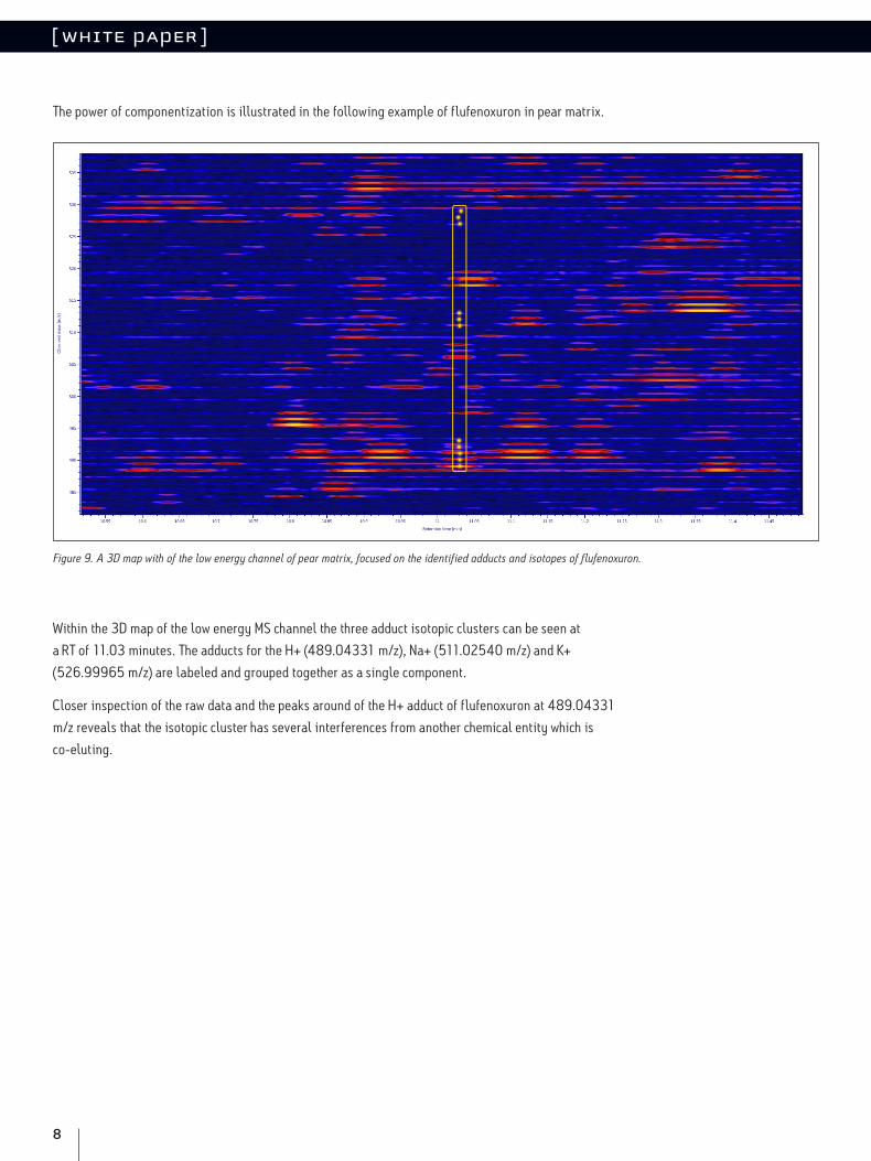
The power of componentization is illustrated in the following example of flufenoxuron in pear matrix.

Within the 3D map of the low energy MS channel the three adduct isotopic clusters can be seen at

a RT of 11.03 minutes. The adducts for the H+ (489.04331 m/z), Na+ (511.02540 m/z) and K+

(526.99965 m/z) are labeled and grouped together as a single component.

Closer inspection of the raw data and the peaks around of the H+ adduct of flufenoxuron at 489.04331

m/z reveals that the isotopic cluster has several interferences from another chemical entity which is

co-eluting.

Figure 9. A 3D map with of the low energy channel of pear matrix, focused on the identified adducts and isotopes of flufenoxuron.

9

The componentization algorithm can differentiate co-eluting species from the flufenoxuron isotopic

cluster. Assuming we are dealing with a singly charged species, the interfering peaks cannot be part of

the 1 Da isotopic difference pattern for flufenoxuron and must therefore be part of a separate isotopic cluster.

Figure 10. The raw mass spectrum (top) and the mass measured spectrum (bottom) for the H+ adduct of Flufenoxuron in pear matrix. The masses belonging to the Flufenoxuron isotopic cluster are highlighted in yellow in the mass measured spectrum.

10

As a further illustration of the power of componentization, the following diagram shows the two

co-eluting masses identified as separate candidate components.

Figure 11. A 3D map with the low energy channel of pear matrix, focused on the co-eluting candidate component at 491.3840 m/z.

11

The following example shows how componentization aligns the candidate components across the two

MSE functions even in complex matrices.

Figure 12. The low and high-energy component spectra graphs of the pesticide Dicrotophos in red pepper matrix.

In the low energy component spectrum (top) the isotopic clusters for the three identified adducts

(H+, Na+ and K+) are highlighted by the green shading. The aligned high-energy product ions are shown

in the bottom spectrum. In this case, the three confirmatory products ions are labeled. As with the

previous examples, both the low and high-energy channels show very clean spectra.

Waters Corporation 34 Maple Street Milford, MA 01757 U.S.A. T: 1 508 478 2000 F: 1 508 872 1990 www.waters.com

Waters and UPLC are registered trademark of Waters Corporation. The Science of What’s Possible and UNIFI are trademarks of Waters Corporation. All other trademarks are the property of their respective owners.

©2013 Waters Corporation. Produced in the U.S.A.April 2013 720004597EN SC-PDF

SUMMARY

This document outlines some of the benefits of the componentization approach in conjunction with MSE data.

It provides a unique and powerful technique for analyzing analytical data. The key benefits include:

■ Organization of complex data

■ Simple data visualization

■ Clean MS spectra

– Separation of co-eluting components

■ Full utilization of product ion information generated

during an MSE data acquisition

■ Full use of MSE datasets, providing both precursor and

product ion information for all components

■ Very little/no need to re-inject samples

■ Can be used to fulfill confirmatory criteria

■ Utilized for the identification of unknowns

– Search for diagnostic or common fragments

– Search for neutral losses

■ Storage of all data, methods and libraries within a

relational database

■ Searchable

■ Accessible to all

■ Helps with future decisions