Complexity Theory in Axiomatic Designweb.mit.edu/pccs/pub/2003/tlee-complexity.pdf · Complexity...

Complexity Theory in Axiomatic Design

by

Taesik Lee

Submitted to the Department of Mechanical Engineeringin partial fulfillment of the requirements for the degree of

Doctor of Philosophy in Mechanical Engineering

at the

MASSACHUSETTS INSTITUTE OF TECHNOLOGY

May 2003

c© Massachusetts Institute of Technology 2003. All rights reserved.

Author . . . . . . . . . . . . . . . . . . . . . . . . . . . . . . . . . . . . . . . . . . . . . . . . . . . . . . . . . . . . . .Department of Mechanical Engineering

May 15, 2003

Certified by. . . . . . . . . . . . . . . . . . . . . . . . . . . . . . . . . . . . . . . . . . . . . . . . . . . . . . . . . .Nam P. Suh

Ralph E & Eloise F Cross Professor of Mechanical EngineeringThesis Supervisor

Accepted by . . . . . . . . . . . . . . . . . . . . . . . . . . . . . . . . . . . . . . . . . . . . . . . . . . . . . . . . .Ain Sonin

Chairman, Department Committee on Graduate Students

Complexity Theory in Axiomatic Design

by

Taesik Lee

Submitted to the Department of Mechanical Engineeringon May 15, 2003, in partial fulfillment of the

requirements for the degree ofDoctor of Philosophy in Mechanical Engineering

Abstract

During the last couple of decades, the term complexity has been commonly found inuse in many fields of science, sometimes as a measurable quantity with a rigorous butnarrow definition and other times as merely an ad hoc label. With an emphasis onpragmatic engineering applications, this thesis investigates the complexity conceptdefined in axiomatic design theory to avoid vague use of the term ’complexity’ inengineering system design, to provide deeper insight into possible causes of complexity,and to develop a systematic approach to complexity reduction.

The complexity concept in axiomatic design theory is defined as a measure ofuncertainty in achieving a desired set of functional requirements. In this thesis, itis revisited to refine its definition. Four different types of complexity are identi-fied in axiomatic design complexity theory: time-independent real complexity, time-independent imaginary complexity, time-dependent combinatorial complexity andtime-dependent periodic complexity. Time-independent real complexity is equiva-lent to the information content, which is a measure of a probability of achievingfunctional requirements. Time-independent imaginary complexity is defined as theuncertainty due to ignorance of the interactions between functional requirements anddesign parameters. Time-dependent complexity consists of combinatorial complexityand periodic complexity, depending on whether the uncertainty increases indefinitelyor occasionally stops increasing at certain point and returns to the initial level ofuncertainty. In this thesis, existing definitions for each of the types of complexity arefurther elaborated with a focus on time-dependent complexity. In particular, time-dependent complexity is clearly defined using the concepts of time-varying systemranges and time-dependent sets of functional requirements.

Clear definition of the complexity concept that properly addresses the causes ofcomplexity leads to a systematic approach for complexity reduction. As techniques forreducing time-independent complexity are known within and beyond axiomatic designtheory, this thesis focuses on dealing with time-dependent complexity. From the def-inition of time-dependent complexity, combinatorial complexity must be transformedinto periodic complexity to prevent the uncertainty from growing unboundedly. Time-dependence of complexity is attributed to two factors. One is a time-varying system

3

range and the other is a time-dependent set of functional requirements. This the-sis shows that achieving periodicity in time-varying system ranges and maintainingfunctional periodicity of time-dependent sets of functional requirements prevent asystem from developing time-dependent combinatorial complexity. Following this ar-gument, a re-initialization concept as a means to achieve and maintain periodicity ispresented. Three examples are drawn from different fields, tribology, manufacturingsystem, and the cell biology, to support the periodicity argument and illustrate there-initialization concept.

Thesis Supervisor: Nam P. SuhTitle: Ralph E & Eloise F Cross Professor of Mechanical Engineering

Committee Members:Professor Jung-Hoon ChunProfessor Seth LloydDr. Hilario Larry OhDr. Jeffrey Thomas

4

Acknowledgments

I have to confess that writing this section of acknowledgement was indeed most chal-

lenging and exciting at the same time. Looking back last six years of my life at MIT

gave me an overwhelmingly long list of people that more than deserve a place for

their name in this humble thesis.

This thesis would not have been possible without the help of Professor Nam Suh.

Ever since the very first day I met him in the fall of 1997, he has always believed

in what I am doing and trusted what I am able to do, oftentimes more than I do

to myself. That has been the thrust with which I was able to go through so many

ups and downs. Most importantly, knowing his trust and confidence in me made me

comfortable criticizing myself when necessary. He is more than a thesis advisor to

me: a true teacher only those most fortunate can have.

Dr. Hilario Larry Oh is another figure in my life at MIT whose influence goes well

beyond this thesis work. I got to know Larry as my mentor for projects I carried out

under MIT-SVG partnership program, and soon he became the one I discuss almost

everything with. Our conversations, may it be a technical or non-technical, never

ended within thirty minutes, and we really enjoyed bouncing ideas back and forth. In

addition to all the technical lessons he taught me, I will always remember his passion,

creativity, and vision.

I would like to say very special thanks to my other committee members, professor

Jung-Hoon Chun, professor Seth Lloyd, and Dr. Jeffrey Thomas. They helped me

through by guiding my work to be on the right track, providing fresh perspectives,

and raising critical questions. I truly appreciate their support and patience.

Former and current members of the axiomatic design group gave me a great mem-

ory of fun as well as contributions to this thesis. Dr. Derrick Tate was a Ph.D. student

when I joined the group, and offered hands so many times when I needed. Jinpyung

Chung has been my office-mate making my life in 31-061 more than enjoyable, and

most happily made it to Ph.D. degree together at the same time. I am glad that I

have become a close friend with Jason Melvin who consistently showed his ingenuity

5

and many other things that made me want to learn from him. Hrishkesh Deo always

asks critical questions that other people take for granted. I would also like to thank

Dr. Rajesh Jugulum and Dr. Il-Yong Kim for their support and encouragement.

Times spent with my friends – Yongsuk, Sangjun, Sokwoo, Daekeun, Soohaeng,

and all the KGSAME members – here are a big part of my memory at MIT. They are

better persons than I am in many ways, and nurtured me to become a better person.

My parents have been the greatest to me. I know that they are the ones mostly

delighted by my becoming a Ph.D. than anyone else in the world. They are my

teachers, friends, and supporters throughout my entire life. As a parent myself, they

are role models that I would like to see myself being any close to.

The most graceful and exciting things that have happened to me during my years

at MIT are my becoming a husband of Alice Haeyun Oh and a father of the most

precious girl Herin. This thesis would not have any meaning without them in my life.

Alice is the one that made this thesis possible. I cannot say in words how much I love

Alice and Herin. Ever since they came into my life, they are the reasons of my life.

6

Contents

1 Introduction 19

1.1 General Concept of Complexity . . . . . . . . . . . . . . . . . . . . . 20

1.2 Object of Complexity Measure: Complexity of What? . . . . . . . . 25

1.3 Complexity in System Design . . . . . . . . . . . . . . . . . . . . . . 28

1.4 Objectives: Why do we introduce the concept of complexity? . . . . . 31

1.5 Complexity in Axiomatic Design . . . . . . . . . . . . . . . . . . . . . 33

1.6 Summary . . . . . . . . . . . . . . . . . . . . . . . . . . . . . . . . . 38

2 Time-independent Complexity 41

2.1 Real Complexity . . . . . . . . . . . . . . . . . . . . . . . . . . . . . 42

2.1.1 Information Content in Axiomatic Design and its Computation 42

2.1.2 Information Content and Information Theory . . . . . . . . . 48

2.1.3 Dealing with Real Complexity . . . . . . . . . . . . . . . . . . 51

2.2 Imaginary Complexity . . . . . . . . . . . . . . . . . . . . . . . . . . 54

2.2.1 Ignorance in Design Process . . . . . . . . . . . . . . . . . . . 54

2.2.2 Iteration in Design Process and Imaginary Complexity . . . . 55

2.3 Information Content vs. Complexity . . . . . . . . . . . . . . . . . . 58

2.4 Summary . . . . . . . . . . . . . . . . . . . . . . . . . . . . . . . . . 59

3 Time-dependent Complexity 61

3.1 Time-dependent Complexity . . . . . . . . . . . . . . . . . . . . . . . 62

3.1.1 Time-varying System Range . . . . . . . . . . . . . . . . . . . 63

3.1.2 Unpredictability of Functional Requirements in Future . . . . 69

7

3.2 Functional Periodicity . . . . . . . . . . . . . . . . . . . . . . . . . . 76

3.3 Summary . . . . . . . . . . . . . . . . . . . . . . . . . . . . . . . . . 79

4 Periodicity, Predictability and Complexity 81

4.1 Combinatorial vs. Periodic Complexity . . . . . . . . . . . . . . . . . 82

4.2 Transformation of Complexity . . . . . . . . . . . . . . . . . . . . . . 83

4.2.1 Time-varying System Range . . . . . . . . . . . . . . . . . . . 84

4.2.2 Time-dependent Functional Requirement . . . . . . . . . . . . 87

4.3 Summary . . . . . . . . . . . . . . . . . . . . . . . . . . . . . . . . . 97

5 Periodicity in a Simple Manufacturing System 101

5.1 Background: Scheduling of a Cluster Tool . . . . . . . . . . . . . . . 102

5.1.1 Throughput Rate of a Cluster Tool . . . . . . . . . . . . . . . 102

5.1.2 Scheduling for Deterministic System . . . . . . . . . . . . . . 104

5.2 Maintaining a Periodicity in a Manufacturing System . . . . . . . . . 111

5.2.1 Example: Wafer Processing System . . . . . . . . . . . . . . . 112

5.3 Summary . . . . . . . . . . . . . . . . . . . . . . . . . . . . . . . . . 129

6 Periodicity in a Biological System: The Cell Cycle 133

6.1 Background: Cells . . . . . . . . . . . . . . . . . . . . . . . . . . . . 134

6.1.1 Cell structure and the Cell Cycle . . . . . . . . . . . . . . . . 135

6.1.2 Regulating the Cell Cycle: Cyclin and Cdk . . . . . . . . . . . 137

6.1.3 Transition of Phases in the Cell Cycle . . . . . . . . . . . . . . 140

6.2 Identifying Functional Requirements in the Cell Cycle . . . . . . . . . 143

6.2.1 Functional Decomposition for G1 phase . . . . . . . . . . . . . 144

6.3 Centrosome Cycle . . . . . . . . . . . . . . . . . . . . . . . . . . . . . 152

6.3.1 Centrosome: Microtubule Organizing Center . . . . . . . . . . 153

6.3.2 The Centrosome Cycle . . . . . . . . . . . . . . . . . . . . . . 155

6.4 Synchronization of Centrosome Cycle and Chromosome Cycle . . . . 157

6.5 Summary . . . . . . . . . . . . . . . . . . . . . . . . . . . . . . . . . 162

8

7 Geometric Periodicity in Designing Low Friction Surface 165

7.1 Background: Mechanism of Friction . . . . . . . . . . . . . . . . . . . 165

7.2 Introducing Periodicity . . . . . . . . . . . . . . . . . . . . . . . . . . 167

7.2.1 Undulated Surface . . . . . . . . . . . . . . . . . . . . . . . . 168

7.3 Summary . . . . . . . . . . . . . . . . . . . . . . . . . . . . . . . . . 170

8 Conclusions 171

8.1 Complexity in Axiomatic Design . . . . . . . . . . . . . . . . . . . . . 171

8.2 Reduction of Complexity . . . . . . . . . . . . . . . . . . . . . . . . . 173

8.3 Suggestions for Future Research . . . . . . . . . . . . . . . . . . . . . 175

9

List of Figures

1-1 Order, midpoint between order and disorder, and disorder. Figure is

taken from [1] . . . . . . . . . . . . . . . . . . . . . . . . . . . . . . . 21

1-2 General complexity concept in the context of engineering system . . . 31

1-3 Representation of a design in axiomatic design theory . . . . . . . . . 34

2-1 ps is the probability that a functional requirement (FR) is within the

specified design range. . . . . . . . . . . . . . . . . . . . . . . . . . . 43

2-2 2-FR joint probability density function, f(FR1, FR2) . . . . . . . . . 45

2-3 (a)Information content vs. (b)Entropy . . . . . . . . . . . . . . . . . 50

2-4 Design iteration can be non-converging by (a) selecting inappropriate

DP for FR or (b) singularity . . . . . . . . . . . . . . . . . . . . . . . 56

3-1 Time-varying system range for a single FR . . . . . . . . . . . . . . . 64

3-2 (a) Joint p.d.f. of (FR1, FR2) is defined over the parallelograms, (b)

marginal p.d.f. of FR2, and (c) marginal p.d.f. of FR1 . . . . . . . . 65

3-3 (a) Modified joint p.d.f. of (FR1, FR2) is defined over the parallelo-

grams, (b) marginal p.d.f. of FR2, and (c) marginal p.d.f. of FR1 . . 66

3-4 Cause-and-effect diagram . . . . . . . . . . . . . . . . . . . . . . . . . 67

3-5 Knob design example (adapted from [2]) . . . . . . . . . . . . . . . . 69

3-6 Desired FR values are changing as a function of time, and thus dynamic

FR. From design perspective, however, T*(t) is not different from

T**(t). . . . . . . . . . . . . . . . . . . . . . . . . . . . . . . . . . . . 70

3-7 A representation that separates design process and operational signal

flow. Time-dependence is now part of the input instead of FR. . . . . 71

11

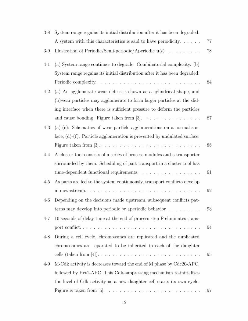
3-8 System range regains its initial distribution after it has been degraded.

A system with this characteristics is said to have periodicity. . . . . . 77

3-9 Illustration of Periodic/Semi-periodic/Aperiodic u(t) . . . . . . . . . 78

4-1 (a) System range continues to degrade: Combinatorial complexity. (b)

System range regains its initial distribution after it has been degraded:

Periodic complexity. . . . . . . . . . . . . . . . . . . . . . . . . . . . 84

4-2 (a) An agglomerate wear debris is shown as a cylindrical shape, and

(b)wear particles may agglomerate to form larger particles at the slid-

ing interface when there is sufficient pressure to deform the particles

and cause bonding. Figure taken from [3]. . . . . . . . . . . . . . . . 87

4-3 (a)-(c): Schematics of wear particle agglomerations on a normal sur-

face, (d)-(f): Particle agglomeration is prevented by undulated surface.

Figure taken from [3]. . . . . . . . . . . . . . . . . . . . . . . . . . . . 88

4-4 A cluster tool consists of a series of process modules and a transporter

surrounded by them. Scheduling of part transport in a cluster tool has

time-dependent functional requirements. . . . . . . . . . . . . . . . . 91

4-5 As parts are fed to the system continuously, transport conflicts develop

in downstream. . . . . . . . . . . . . . . . . . . . . . . . . . . . . . . 92

4-6 Depending on the decisions made upstream, subsequent conflicts pat-

terns may develop into periodic or aperiodic behavior. . . . . . . . . . 93

4-7 10 seconds of delay time at the end of process step F eliminates trans-

port conflict. . . . . . . . . . . . . . . . . . . . . . . . . . . . . . . . . 94

4-8 During a cell cycle, chromosomes are replicated and the duplicated

chromosomes are separated to be inherited to each of the daughter

cells (taken from [4]). . . . . . . . . . . . . . . . . . . . . . . . . . . . 95

4-9 M-Cdk activity is decreases toward the end of M phase by Cdc20-APC,

followed by Hct1-APC. This Cdk-suppressing mechanism re-initializes

the level of Cdk activity as a new daughter cell starts its own cycle.

Figure is taken from [5]. . . . . . . . . . . . . . . . . . . . . . . . . . 97

12

4-10 (a) Combinatorial complexity. (b) Periodic complexity: re-initialization 98

5-1 Cluster tool with seven process steps: A cluster tool is characterized

by a a group of modules organized around a transporter. . . . . . . . 103

5-2 If there is no process constraint and thus delays are allowed at all the

process steps, there exists a trivial schedule that achieves FP ∗. In the

figure, horizontal arrows indicate delay times, and all the process times

are extended to have the same length as bottleneck process. . . . . . 107

5-3 (a) 1-part cycle gives a throughput rate of 113

while 2-part cycle shown

in (b) yields higher throughput rate of 110

. . . . . . . . . . . . . . . . 109

5-4 Subsystem X and Y are joined together to subject wafers to a series of

processes. . . . . . . . . . . . . . . . . . . . . . . . . . . . . . . . . . 112

5-5 Part-flow timing diagram. Each row represents the individual panels

being processed by different machines. Transport task (3 4)-(9 10) and

(1 2)-(5 6) are in conflicts. . . . . . . . . . . . . . . . . . . . . . . . . 116

5-6 10 seconds post-process delay times at process b and d resolve the

conflicts. . . . . . . . . . . . . . . . . . . . . . . . . . . . . . . . . . . 117

5-7 Steady state scheduling solution with CTY at constant 90 seconds . . 118

5-8 Variation in subsystem Y’s cycle time . . . . . . . . . . . . . . . . . . 120

5-9 Information at the instant of re-initialization . . . . . . . . . . . . . . 121

5-10 [1 2], [3 4] are pre-fixed. No-transport-time is indicated by X’s. . . . . 121

5-11 Resulting schedule for case 2 . . . . . . . . . . . . . . . . . . . . . . . 122

5-12 Steady state operation with sending period of 70 seconds . . . . . . . 123

5-13 . . . . . . . . . . . . . . . . . . . . . . . . . . . . . . . . . . . . . . . 124

5-14 . . . . . . . . . . . . . . . . . . . . . . . . . . . . . . . . . . . . . . . 124

5-15 . . . . . . . . . . . . . . . . . . . . . . . . . . . . . . . . . . . . . . . 124

5-16 . . . . . . . . . . . . . . . . . . . . . . . . . . . . . . . . . . . . . . . 124

5-17 . . . . . . . . . . . . . . . . . . . . . . . . . . . . . . . . . . . . . . . 125

5-18 . . . . . . . . . . . . . . . . . . . . . . . . . . . . . . . . . . . . . . . 125

5-19 . . . . . . . . . . . . . . . . . . . . . . . . . . . . . . . . . . . . . . . 125

13

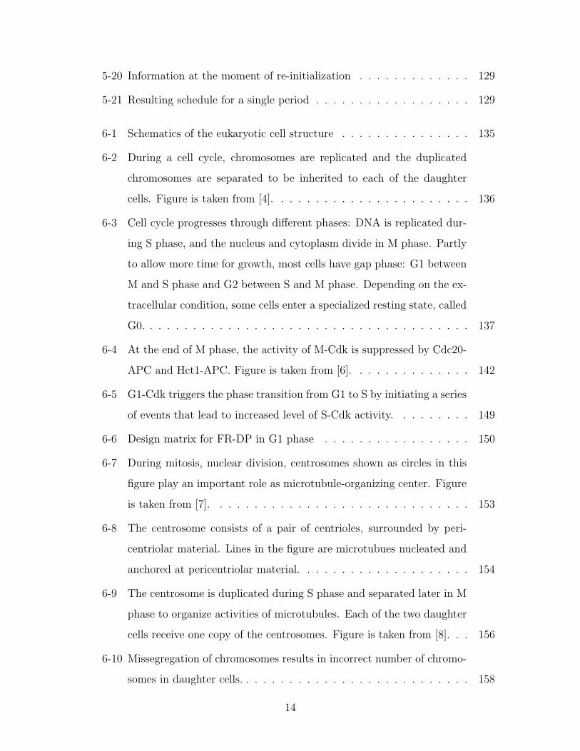
5-20 Information at the moment of re-initialization . . . . . . . . . . . . . 129

5-21 Resulting schedule for a single period . . . . . . . . . . . . . . . . . . 129

6-1 Schematics of the eukaryotic cell structure . . . . . . . . . . . . . . . 135

6-2 During a cell cycle, chromosomes are replicated and the duplicated

chromosomes are separated to be inherited to each of the daughter

cells. Figure is taken from [4]. . . . . . . . . . . . . . . . . . . . . . . 136

6-3 Cell cycle progresses through different phases: DNA is replicated dur-

ing S phase, and the nucleus and cytoplasm divide in M phase. Partly

to allow more time for growth, most cells have gap phase: G1 between

M and S phase and G2 between S and M phase. Depending on the ex-

tracellular condition, some cells enter a specialized resting state, called

G0. . . . . . . . . . . . . . . . . . . . . . . . . . . . . . . . . . . . . . 137

6-4 At the end of M phase, the activity of M-Cdk is suppressed by Cdc20-

APC and Hct1-APC. Figure is taken from [6]. . . . . . . . . . . . . . 142

6-5 G1-Cdk triggers the phase transition from G1 to S by initiating a series

of events that lead to increased level of S-Cdk activity. . . . . . . . . 149

6-6 Design matrix for FR-DP in G1 phase . . . . . . . . . . . . . . . . . 150

6-7 During mitosis, nuclear division, centrosomes shown as circles in this

figure play an important role as microtubule-organizing center. Figure

is taken from [7]. . . . . . . . . . . . . . . . . . . . . . . . . . . . . . 153

6-8 The centrosome consists of a pair of centrioles, surrounded by peri-

centriolar material. Lines in the figure are microtubues nucleated and

anchored at pericentriolar material. . . . . . . . . . . . . . . . . . . . 154

6-9 The centrosome is duplicated during S phase and separated later in M

phase to organize activities of microtubules. Each of the two daughter

cells receive one copy of the centrosomes. Figure is taken from [8]. . . 156

6-10 Missegregation of chromosomes results in incorrect number of chromo-

somes in daughter cells. . . . . . . . . . . . . . . . . . . . . . . . . . . 158

14

6-11 Centrosomal abnormalities are common in human tumor cells: Tumor

colon tissues(b) contains amplified centrosomes compared to normal

cells(a), indicated by bright spots; Human prostate tumor(d),(e) has

multipolar spindles shown by dark spots while normal cell(c) has a

bipolar spindle. Images are taken from [8]. . . . . . . . . . . . . . . . 158

6-12 (a) A schematic comparison of centrosome cycle and chromosome cycle.

This figure is taken from [8]. (b) Coordination of two cycles bears

resemblance to the manufacturing system example presented in chapter

5. . . . . . . . . . . . . . . . . . . . . . . . . . . . . . . . . . . . . . . 160

6-13 Synchronization of chromosome and centrosome cycles involve at least

three mechanisms: S-Cdk acting as a signaling agent to initiate both

cycles at the same time, checkpoints to ensure the completion of du-

plication process in both cycles, and Cdk-inhibitory mechanism to ini-

tialize the level of Cdk at the end of the cell cycle. . . . . . . . . . . . 161

7-1 A spherical particle entrapped at the sliding interface is indenting into

(a) two identical metals, (b) soft metal when one metal is much harder

than the other. The dimensions of the particles are shown in (c).

Figure is taken from [9]. . . . . . . . . . . . . . . . . . . . . . . . . . 166

7-2 Friction coefficient due to plowing component increases nonlinearly as

a function of the depth of penetration of the wear particle. Figure is

taken from [9]. . . . . . . . . . . . . . . . . . . . . . . . . . . . . . . . 167

7-3 (a) An agglomerate wear debris is shown as a cylindrical shape, and

(b)wear particles may agglomerate to form larger particles at the slid-

ing interface when there is sufficient pressure to deform the particles

and cause bonding. Figure is taken from [3]. . . . . . . . . . . . . . . 168

7-4 (a)-(c): Schematics of wear particle agglomerations on a flat surface,

(d)-(f): Particle agglomeration is prevented by undulated surface. Fig-

ure is taken from [3]. . . . . . . . . . . . . . . . . . . . . . . . . . . . 169

15

7-5 Friction coefficient versus sliding distance in copper on (a)flat Zinc

surface and (b)undulated zinc, sliding at 2.5N normal load and 0.01m/s

sliding speed [3]. . . . . . . . . . . . . . . . . . . . . . . . . . . . . . 170

8-1 Four types of complexity are identified in axiomatic design. Depending

on the uncertainty’s time-dependence, it is divided into time-independent

and time-dependent complexity. Time-independent complexity con-

sists of real and imaginary complexity, and time-dependent complexity

has combinatorial and periodic complexity. . . . . . . . . . . . . . . . 172

16

List of Tables

1.1 Various complexity definitions/measures and their intended applica-

tion . . . . . . . . . . . . . . . . . . . . . . . . . . . . . . . . . . . . 27

3.1 Marginal probability of success for FR2 increases while the overall

probability of success decreases. . . . . . . . . . . . . . . . . . . . . . 66

5.1 Parameters for Case 1 . . . . . . . . . . . . . . . . . . . . . . . . . . 115



6.1 Cyclins and their Cdk partners for vertebrate cell and budding yeast [10]138

17

Chapter 1

Introduction

The term, complexity is commonly found in use throughout virtually all fields of

science including physics, biology, sociology, to name a few. In the discipline of

engineering, the term “complex” or “complexity” are also getting popular as the

objects of its study tend to demand unprecedented way of treatments in many ways.

Despite the abundance of currently available diverse definitions and descriptions,

this thesis introduces still another concept that shares the name, complexity. The

scope of complexity concept discussed in this thesis remains mainly in the pragmatic

domain, particularly in the area of engineering system design. The peculiarity of the

complexity concept discussed in this thesis lies in its emphasis on the relative aspect

with respect to the functional requirements, i.e. what we want to achieve/know. It

has its theoretical basis on axiomatic design theory. In this introductory chapter,

common notions of complexity concept are discussed with some examples, followed

by a brief survey of some of the formal complexity study. Next, the complexity is

discussed in relation to engineering design. In particular, the concept of complexity

defined in axiomatic design theory is briefly introduced, and the difference in its

perspective from the others is emphasized.

19

1.1 General Concept of Complexity

Arguably the most fundamental question around the subject matter is “what is com-

plexity?” What makes us to judge that an entity – may it be a system, phenomenon,

problem, etc. – is complex? Perhaps in its most naıve sense, it is the difficulty in

dealing with1 the entity under consideration. Indeed, many of formal and informal

complexity discussions are centered around this basic notion of difficulty. Efforts are

focused on characterizing and quantifying the difficulty. It is not surprising to see

that there is no consensus on the definition of complexity so far. For example, some

people define complexity as a degree of disorder. Others use the minimum length of

description to define complexity. The amount of resource such as time or memory to

solve a certain problem is another example of complexity definition. Combination of

these definitions yields still other definitions. Before discussing some of the existing

concept of complexity, let us begin with a few examples to highlight some of the issues

in defining the concept2.

• A cell vs. the potato it was taken from

If the complexity is some absolute quantity inherent to a system, it would make

most sense to say that a subsystem cannot be more complex than the system that

it is a part of. For example, regardless of the complexity of a cell, an organism

is more, or at least no less, complex than a cell since a cell cannot take away the

complexity of other cells. However, that is not obvious any more when viewed from

different frameworks. It seems natural to judge a cell under a microscope to be much

more complex than the potato it was taken from. That is because human beings

intrinsically choose different framework with a different level of granularity to filter

out unnecessary information. This example suggests that defining problem itself play

an important role in understanding complexity and that absolute complexity concept

could be inappropriate way of looking at the problem.

1This vague expression is intentionally used because depending on the context, it could be ‘un-derstanding’, ‘solving’, ‘modeling’, etc.

2These examples are taken from [11]

20

Figure 1-1: Order, midpoint between order and disorder, and disorder. Figure istaken from [1]

• Motion of the planets

One may want to ascribe its complexity to the system of planets itself and quantify

its absolute value. That can possibly be done by relying on some framework for which

privilege is claimed, e.g. entropy. As a consequence of doing so, one would have to

consider all feasible models as equally complex since a model is simply a description

of what is being modeled. Thus, no matter what language is used to model the

system, the complexity of a system itself should remain same. However, clearly

different degree of complexity, in some sense, is perceived depending on the required

specificity and the models chosen to describe a system. For example, motion of the

planets will be considered extremely complex to describe if the required error level

is prohibitively tight. On the other hand, it can be as simple as a drawing on the

back of the envelop if all we need is a very general description. Perceived level of

complexity also depends on the model chosen to describe the system. For example,

the exact motions of the planets seem so complicated when we describe them in terms

of epi-cycles but much simpler in terms of ellipses. From this example, we can see

that the absolute complexity concept can potentially overlook important part of the

problem such as specificity and the role of model and tool.

• Ordered/disordered pattern

When asked which of the above three patterns in figure 1-1 is most complex,

we can possibly consider how difficult it is to represent each pattern or to generate

21

them. Instead of a single right answer, there could be several different opinions

depending on the assumptions or a particular perspective held by an observer. For

example, one might say the second (middle) is the most complex pattern since both

the first and the third have simple rules behind – simple repetition and randomness

(no-rule), respectively –, and thus easy to generate. On the other hand, in terms

of representation, the third figure is most complex because there is no regularity

at all. Therefore, it is almost incompressible, which means the amount of required

information is that of raw data. This example shows that depending on the particular

aspect of the problem, the same system – pattern in this case – can present different

level of complexity.

As shown in the above examples, there could be a large ambiguity in discussing

the concept of complexity unless it is carefully delineated: for example, the language

(model) chosen to describe the object, scale or level of detail, specificity, and particu-

lar aspect being considered must be part of the complexity discussion. Even though

the different concepts share the same name, complexity, and probably address same

fundamental question of difficulty, they rely on different assumptions and therefore

lead to different implications. To avoid such ambiguity, many of the formal complex-

ity research have attributed the complexity to some absolute quantity by considering

only one aspect of the problem, considering the minimal size, or limiting its scope

to a certain type of problems/systems. This will be evident by looking at the well-

established complexity measures. Formal ways of discussing the subject of complexity

fall largely into three classes of definition: probabilistic, algorithmic, and computa-

tional approaches. Here, a few examples in each of three classes are presented.3

Examples of the first class include Boltzmann-Gibbs entropy and Shannon Infor-

mation. Equation 1.1 is the general form of the definition of entropy in statistical

mechanics:

S = −k∑

pi ln pi (1.1)

3For more comprehensive survey of complexity measures, readers are recommended to refer to[11].

22

where k is an arbitrary constant that depends on the unit of entropy, and pi is the

probability that particle ‘i’ will be in a given microstate for a certain macrostate.

Since the advent of statistical mechanics in the late 1800’s and early 1900’s, en-

tropy, which has its root in the second law of thermodynamics, has been considered

an effective measure of disorder. The concept gained a statistical interpretation, i.e.

a measure of uncertainty about the actual microscopic state of a system. This aspect

of entropy interpretation was enriched when Shannon introduced the information the-

ory in the middle of twentieth century [12],[13],[14]. It is by no means a coincidence

that Shannon’s entropy shares the same mathematical formula as Shannon proved in

[15]. Not only is the mathematical formula common to both concepts, but also is the

core interpretation: they measure uncertainty. It is this statistical interpretation that

enabled the concept of entropy to reach the realm outside the thermodynamics and

to have become one of the norms in the complexity discussion later on. The central

idea of this approach is that the more disordered a system is, the more information

is needed to describe it and thus the system is more complex.

Algorithmic complexity4 and logical depth are the examples of the second kind.

Algorithmic complexity, sometimes called AIC (Algorithmic Information Content) or

Kolmogorov complexity, is defined for a string of symbols, x, as the length of the

shortest program that instructs a Turing machine to produce output x and then halt

[17],[16]. Formally,

KU(x) = minp:U(p)=x

l(p)

where U is a universal computer (or Turing machine), p is any program that print

x and halt, and l(p) is the length of a program. A Turing machine is an abstract

representation of a computing device. It uses an infinite tape as its unlimited mem-

ory. It has a read/write head that can read and write symbols and move around on

the tape. Initially the tape contains only the input string and is blank everywhere

4The ideas of this algorithmic complexity, i.e. minimal length of description, were put forthindependently and almost simultaneously by Kolmogorov, Solomonoff and Chaitin [16]. Thus, it iscommonly referred to as Kolmogorov complexity or Kolmogorov-Solomonoff-Chaitin complexity.

23

else. The machine scans the tape, writes information on the tape if necessary, and

changes its state. It continues computing until it decides to produce an output. From

the definition, we see that the algorithmic complexity does not require probability

distribution when defining complexity. Another example of algorithmic definition of

complexity is logical depth, which is a variation of algorithmic complexity. Bennet[18]

defines logical depth as the running-time to generate an object in question with near-

incompressible program. Strictly, the depth of a string x at level s is

Ds(x) = min {T (p)| |p| − |p∗| < s ∧ U(p) = x}

where T (p) is the time taken by program p, and p∗ is the shortest program that

computes x. It is thus combination of Kolmogorov complexity and computational

complexity which is discussed below.

The last class is computational complexity. The computational complexity is the

amount of time, memory, or other resources required for solving a computational

problem with respect to the size of a problem [17]. This is a very useful concept when

analyzing computational algorithms. Computational algorithms are evaluated based

on the running time to reach a solution for a problem. In turn, once the best algorithm

is discovered for a certain type of problems, such problems are categorized to different

classes of computational complexity, e.g. class P, NP, etc. Here, the term complexity

is equated to the difficulty of solving a problem strictly in terms of computational

resources, given the best algorithm known so far. Therefore it has well-bound scope

of application: the study of computation and computational algorithm.

As mentioned earlier, the desire that has led to the above formulation is to at-

tribute complexity purely objectively to a physical process or a system and thereby

eliminate potential ambiguity in the concept. Such absolute-complexity standpoint

excludes the relative aspect of the problem, which is indeed a crucial part of the

problem from a pragmatic standpoint. From a pragmatic perspective, complexity is

a quantity or quality perceived by an observer (or designer, solver, etc.). Therefore,

various factors involved in the act of observation must be taken into account in as-

24

sessing the complexity. From this reasoning, some claim that the complexity is more

critically dependent on the choice of a particular model rather than what is being

modeled itself. In other words, complexity can be defined only in relation to scientific

modeling. In that sense, the complexity is defined as “the difficulty associated with a

model’s form when given almost complete information about the data it formulates”

[11], or “the property of a real world system that is manifest in the inability of any one

formalism being adequate to capture all its properties” [19]. The previous examples

of “planet motion” and “cell vs. potato” may illustrate the point.

After all, from axiomatic design standpoint whose emphasis is pragmatically on

design, one of the most valuable outcomes of the study of complexity would be the

deep insight into the causes of complexity, but it can hardly be found in the exist-

ing complexity discussions. Substantial part of complexity study is to quantify (or

sometimes just describe) the difficulty associated with the object under question. It

is as much or even more of interest in engineering domain to know what causes the

difficulty and, from there, to figure out how to actually reduce the level of difficulty.

1.2 Object of Complexity Measure: Complexity of

What?

An attempt to answering the first question – what is the complexity? – leads to

another question: “of what entity are we discussing the complexity?” To list a few,

it could be the complexity of a natural system, phenomenon, artifact, or a computa-

tional problem. In discussing complexity, especially complexity measure, the object

of being complex – the entity that is judged to be complex – is oftentimes implicit.

A metric that works very well for a certain subject may not be suitable at all for

the complexity of other subjects. Indeed, that accounts for much of the confusion,

and explains why a survey of wide range of complexity definitions seems unproduc-

tive. The question, ‘what is complexity’ is ambiguous until the target of the question

is specified. Once we specify the object to which the concept of complexity is ap-

25

plied, then the first question can be rephrased such that it becomes a more tangible

question. For example, why is ‘this pattern’ complex, and how complex? What is

the complexity of ‘this computational problem’? Depending on the context of the

complexity question, it focuses on a certain aspect of the problem and accordingly

requires different formulation. Consequently, it carries different meaning with, possi-

bly, a unique metric. Therefore, one of the very first steps in discussing the subject

matter of complexity is to clarify the object of the question, i.e. ‘complexity of what?’

Table1.1 summarizes such relationship. In the left column listed are various def-

initions or measures5 of complexity, and the right column shows what is considered

by the relevant complexity concept. As you can see, some of the complexity con-

cept, for example cognitive complexity, has a very specific target application that is

behavioral personality. On the other hand, a size as a complexity measure is very

general concept that can be used in many different context: for example, size of rules

is used to represent complexity of a pattern, and size (number) of variables to indicate

complexity of modeling.

Even without knowing details about the individual complexity measures listed

in the table, one can immediately tell that many of the complexity measures have

limited scope, which, if not properly recognized, would create unnecessary confusion.

For example, albeit they share part of their name, cognitive complexity is not even

close to Kolmogrov complexity in any dimension. The objects of the study for two

complexity concepts are so remote that each measure aims completely different aspect

of the problem. In many cases, an attempt to use one complexity definition for

different object results in an inappropriate force-fitting. Therefore, any complexity

definition or measure must be understood in the context of its intended use, and

care should be given when discussing different kinds of complexity definitions and

measures.

Secondly, many of the measures address the complexity indirectly. Some of them

are potentials that can lead to large complexity but not necessarily. For example,

‘size’ of the problem, i.e. number of variables or dimensions, is the potential at-

5These complexity definitions and/or measures are taken from Edmonds’ survey [11].

26

Complexity definition/measure ObjectKolmogorov complexity (AIC), Shannon’s in-formation/entropy

An object with information, e.g. stringbit, pattern

Size (size in many different context) GeneralVariety, Irreducibility (Biological) SystemDimension, Ability to surprise, Irreducibility System (as an object of modeling)Connectivity, Cyclomatic number, Ease of de-composition

System with network characteristic(components are interconnected)

Stochastic complexity Physical processes or dataSize of rules (or grammars), Midpoint betweenorder and disorder, Logical depth, Sophistica-tion

Pattern (if viewed as a result of pro-duction rules in a language)

Boltzmann-Gibson entropy, AIC, Improbabil-ity, Thermodynamic depth, Total information

(Thermodynamic) System or state

Sober’s minimum extra information, Expres-sivity, Logical complexity, Kemeny’s mea-sures, Goodman’s complexity

Statement, Language, (Theory)

Size of minimal characteristic matrix LogicCognitive complexity Personality, Cognitive/behavioralTime (processing/execution/preparation) A taskResources (time/memory/others), Ignorance,Information in loose sense

Solving a problem

Table 1.1: Various complexity definitions/measures and their intended application

27

tribute for a complex system, but having a large size does not necessarily mean that

the system is complex. One can augment this simple measure by including additional

features such as connectivity, cyclomatic number, but still it cannot be the sufficient

condition for being complex. Some of them are more of an indicator or symptom

of being complex. Such measures include computational time, length of description

(information), irreducibility, logical depth, and ease of decomposition. They are use-

ful in comparing two or more objects that present same symptoms. For example,

computational time measure enables us to say that problem A is more complex than

problem B because it takes longer time to solve. However, these concepts generally

have a strict scope due to the fact that they tend to focus on a specific symptom.

Lastly, based on the observation on table 1.1, it seems that for most of the com-

plexity concepts, the name, complexity has been given to those concepts and measures

ad hoc. In other words, in the course of the study of particular subject, the associ-

ated difficulty – in any sense – is termed as complexity of the entity and a suitable

metric is provided. It explains very well the lack of universal complexity definition

and measure. That, in turn, justifies our attempt to introduce another concept of

complexity.

1.3 Complexity in System Design

Having emphasized the significance of clarifying the object of complexity measure,

this thesis limits the scope within engineered system, a system being a collection of

physical/non-physical entities (design parameters) that cooperatively deliver overall

functional requirements. This would include typical engineering systems, biological

systems, and economic systems, while excluding patterns, logic, and computational

problems. It will be discussed in section 1.5 that the complexity concept presented in

the thesis is based on the axiomatic design framework. In this section, current notion

of complexity in the context of engineering system (design) is briefly discussed.

In engineering system design, the term ‘complex’ is often considered as a synonym

28

of ‘complicated’ just as they are in English dictionaries.6 However, if we want to be

precise in using the terminologies, there is a subtle difference in their connotations.

A distinction can be made between the two by emphasizing the aspect of ‘interde-

pendence’ of complex system. Complex systems have components whose behavior is

dependent on the interactions with other components in the system. On the other

hand, the interactions of the components of complicated systems are simply additive,

and thus their behavior is generally independent of those interactions. In other words,

the properties of an individual component in a complex system cannot be determined

without considering the whole system, whereas they can be determined from local

consideration for a complicated system. Yet, the use of the terminologies is relatively

casual and so is the meaning of them. Thus they are considered as synonyms by and

large. Little work has been done to define ‘complexity’ in the context of engineering

design, and we simply depend on its ordinary dictionary definition. Despite the lack

of formal definition, it is well accepted that modern engineering systems are becom-

ing more and more ‘complex’. Typical examples of using the term ‘complexity’ or

‘complex’ would be ‘Boeing-737 is a complex system’; ‘An automobile is less complex

than an aircraft’; ‘This manufacturing system is complex’; ‘A large system has large

complexity’; ‘A system with modular design has low complexity.’

We can immediately generate a list of intuitive reasons that lead to the above

example sentences.

• has a large physical structure (e.g. huge part count)

• performs many different functions as a result of a collective behavior

• has multi-level interactions or chained interactions among its constituents

• does not have clear cause-effect relations

• is difficult to understand/make

The first thing you may notice from the list is that the last one is the essential

attribute of so-called complex system and the other four are potential causes of it.

6complex: Consisting of parts or elements not simply coordinated, but some of them involved invarious degrees of subordination; complicated, involved, intricate; not easily analyzed or disentan-gled. complicated: Consisting of an intimate combination of parts or elements not easy to unravelor separate; involved, intricate, confused. From Oxford English Dictionary 2nd edition, 1989.

29

Without difficulty in understanding (or making, operating, etc.), a system is not said

to be complex. For example, the intricate interactions among its component is not

sufficient reason for a system to be complex. Secondly, the notion of complexity, in

the context of engineering system design, almost always implies the system concept.

Indeed, the first three are commonly considered as the attributes of a ‘system.’ Thus,

the complexity is a property of a system. Then, the last two will be what distinguishes

between a complex system and non-complex system.

Having said so, complexity is the property of a system that makes it difficult to

understand as a whole through the collection of knowledge about its constituents. Or

in other words, one of the essential characteristics of complex system is its emergent

(or collective) behavior that is not readily understandable/predictable from individual

components’ properties. “Understanding” means being able to explain its causality

and thus being able to predict its behavior (output) given initial conditions (input).

When it is properly understood, one should be able to explain ‘how’ the overall

behavior is produced from the collective behavior of its components. It is particularly

challenging to understand a complex system because “pushing on a system ‘here’

often has effects ‘over there’ due to interdependence of parts.”7 So, the complexity is

a property of a system that makes it difficult to understand the causality between its

overall function or behavior and the components’ properties given external condition

or input. Figure1-2 summarizes such a general concept of complexity.

Although the above paragraph defined complexity based on the common intuitive

reasons why a system is complex, it is merely an elaboration of what is defined in

an ordinary dictionary. Indeed, this loose definition represents general notion of the

complexity in engineering system design as suggested by a couple of examples.

This informality may be an indication of its inclination to pragmatism in engi-

neering domain. With this casual treatment of the subject, the complexity is only a

metaphor to signify the difficulty associated with a system under question. It does

not matter whether the system is truly complex or not, or exactly how complex a

system is. What matters is the particular aspect that the so-judged complex system

7Cited from http://necsi.org/guide/whatis.html

30

COMPLEXITY

Property of a System-Collection of subsystems/elements/parts-Has overall functions that can only result from the collective behavior

Difficult to Understand “HOW” these functions come about

How the interrelationship produces such collective behavior

-Know causality-Be able to predict

Be able to engineer a desired functions

-(minimum) Length of description-(minimum) Amount of time to create

In engineering design domain, how to get to this minimum would be of critical interests

mea

sure

Figure 1-2: General complexity concept in the context of engineering system

has, e.g. large and interconnected structure. The message to convey when saying ‘this

is a complex system’ is most likely that this system is not subject to straightforward

engineering practice. In that sense, the complexity per se is a conceptual (qualitative)

property that may be distinguished by several measurable or observable quantities,

and apparently unavoidable property that must be handled sophisticatedly. Each of

those measurable quantities is the subject of a specific technique. Then the collection

of the activities and the results is abstracted as “coping with complexity.” Therefore,

the study of complexity almost immediately becomes the study of complex systems,

i.e. how to cope with complexity. However, the lack of fundamental definition of the

complexity itself results in failure to address one important question: how to reduce

complexity. Without understanding the complexity itself, we cannot deal with this

critical question. That is why we introduce the complexity in axiomatic design theory.

1.4 Objectives: Why do we introduce the concept

of complexity?

We see that there exist wide range of complexity definitions as briefly discussed in

section 1.1 and 1.2. Despite the abundance of diverse definitions and descriptions

currently available, this thesis still introduces another different concept that shares

31

the common name, complexity. That is justified by the fact that most of the existing

complexity concepts are defined ad hoc per each of the research objectives, and thus

the result of such research is not readily transferable to our concern, i.e. engineering

system design. Not only is it justified, but also the effort is motivated by the lack

of established complexity concept in engineering design domain. The peculiarity of

the complexity concept introduced here lies in its emphasis on the relative aspect

with respect to functional requirements, i.e. what you want to achieve/know. This

complexity concept has its theoretical basis on axiomatic design theory.

The introduction of axiomatic design’s complexity concept is intended to achieve

the following objectives:

• To avoid the vague usage of the term in the engineering design discipline.

As mentioned in section 1.3, the term is commonly used in a vague way within

engineering domain. Such a vague use of the term may be justified by the intrinsic

pragmatism of the discipline. However, it probably has been so simply due to the

lack of proper definition of it. A clear definition of complexity cannot be counter-

productive since it will open up a channel for communication by eliminating the

ambiguity and the confusion caused by it. To this end, the complexity concept defined

in axiomatic design theory can definitely contribute.

• To acquire deeper insight into possible causes of complexity in engineering de-

sign.

The next step of the research is to investigate the potential causes of complexity.

What makes this system complex? Is there a sufficient condition for being complex?

Or a necessary condition? The understanding of the cause of complexity will bear

significant practical implications. Once this insight is gained, it will be reflected to

the design process for complexity reduction.

• To develop a systematic approach to complexity reduction.

32

The ultimate goal of the complexity study here is to develop a systematic ap-

proach to reduce complexity. Note that this objective assumes that the complexity

is a reducible quantity. That is very different from many other complexity concepts

which attribute complexity purely objectively to the physical entity itself. Also, it

implies that the complexity is the consequence of certain causes that are subject to

engineering activities.

This thesis explores the axiomatic design’s complexity concept in detail to make

some progress toward these goals.

1.5 Complexity in Axiomatic Design

The very first appearance of the concept of complexity in axiomatic design can be

found in [20], and two years later came a more detailed discussion as a book chapter

in [2]. Axiomatic design theory8 is centered around the concept of functional require-

ment (FR), design parameters (DP) and their quantitative/qualitative interrelations

represented by design matrix ([DM]). A set of functional requirements, {FR} are the

functional deliverables of the designed artifact, and design parameters {DP} are the

means to achieve the {FR}. Then, [DM] signifies how they are related; it could have

a form of sensitivity, model, transfer function, or qualitative description. Then, a

design is defined as an interplay between functional domain – FR domain – and phys-

ical domain – DP domain –, and it is represented by a hierarchy of {FR}, {DP} and

[DM] as shown in figure 1-3.

There are two design axioms, namely Independence axiom and Information axiom:

Independence Axiom: Maintain the independence of functional re-

quirements

Information Axiom: Minimize the information content

A design that satisfies the two design axioms is considered a good design that

delivers intended functions with minimum information content.

8Those who are not familiar with the subject are recommended to refer to [2]

33

Functional Physical

FR1

FR1.1 FR1.2

FR1.2.1 FR1.2.2

DP1

DP1.1 DP1.2

DP1.2.1 DP1.2.2

��

XO

OX

��

XX

OX

Figure 1-3: Representation of a design in axiomatic design theory

Suh defined complexity in axiomatic design while trying to answer to the ques-

tion “why some sets of {FR} are more difficult to achieve than others?” Having

said the ultimate goal of design is to satisfy the desired functional requirements, the

answer he came up with is ‘complexity’. It is defined as a measure of uncertainty in

achieving a set of desired functional requirements [2]. In other words, complexity is

the property of a design – represented by {FR}, {DP} and [DM] – that makes the

desired functional requirements difficult to achieve (or improbable to satisfy). Note

that uncertainty of achieving desired functional requirement is interpreted as the un-

likelihood of achieving them. Usually, ‘uncertainty’ implies being not sure about the

outcome, and thus uniform probability about the outcome, as in a fair coin toss, is

most uncertain with the least predictability. However, axiomatic design theory is

extremely interested in ‘getting head’ in an arbitrary coin toss, i.e. how ‘likely’ it is

to obtain head in a coin toss. Therefore, when we say ‘it is very uncertain to get

head in a coin toss,’ it means ‘it is very unlikely to get head’ rather than ‘it is not

certain whether we are going to get head or tail.’ In other words, if the probability

of head is 0.001, it is quite certain that the outcome will be the tail side. Saying that

it is very ‘uncertain’ to get head out of the coin toss may sound strange since we are

quite ‘certain’ that we will not get head as the outcome. It is clearer to say it is very

unlikely to get head out of the coin toss. To summarize, “a measure of uncertainty

in achieving desired functional requirement” must be understood as “a measure of

34

un-likelihood of achieving desired functional requirement.

At a first glance, this particular definition of complexity – large complexity means

large uncertainty – may seem counter-intuitive. One might say, for example, bio-

logical systems have been evolved into more and more complex system to cope with

surrounding environment more effectively, i.e. to reduce the uncertainty in achieving

the desired functional requirement – survival. So, uncertainty in achieving a desired

set of functional requirements is reduced as a system becomes more complex. In

other words, as a result of decreasing the uncertainty, systems typically become more

complex. Some extends this argument further to state that complexity is the result

of robustness: ‘the robustness drives the complexity’ [21]. The above argument is

partially right in that as a result of an effort to reduce uncertainty, some physical

quantities tend to increase. Such quantity could be number of components, inter-

connectivity of its network representation, number of functions, etc. But, axiomatic

design’s complexity concept does not necessarily agree with the reasoning that those

quantities represent the complexity. In axiomatic design’s complexity perspective, a

single-cell amoeba can be more complex than a human being with more than tens of

trillions of cells; a bicycle can be more complex than Boeing 737. These seemingly

counter-intuitive statements can be understood when considering its relative aspect

of function-oriented definition. It emphasizes functional view over physical view. Be-

ing physically complicated is not necessarily equated to being complex. It is also a

strictly relative concept while most of us are used to an absolute or objective complex-

ity concept such as size. Axiomatic design complexity can be discussed only after the

system’s functional requirements are properly defined. In other words, the complexity

discussion must be put into some context. On what basis are we discussing the com-

plexity of an amoeba vs. a human being? Recall the cell-potato example presented

early in this chapter. On what basis is the comparison justified? Is it meaningful to

compare a cell with potato within a single framework? Axiomatic design complexity

is always relativised with respect to system’s functional requirements. Complexity

of a system strongly depends on the question we pose. Based on axiomatic design’s

complexity definition, the antonym of ‘complex’ is not ‘simple’ but ‘certain’ in terms

35

of achieving a desired set of functional requirements.

Axiomatic design complexity can also be justified in intuitive sense, i.e. com-

plicated ≈ complex if the realization process, {DP}-{PV} is taken into account.

Achieving FR is essentially a two-step process: come up with means to achieve a

desired set of FRs, and physically realize the mechanism of {DP}→{FR}. If the

embodiment process, {DP}-{PV}, is complicated, then the second step can present

large uncertainty. Take, for instance, a high-precision machine such as a lithography

machine used in semiconductor manufacturing process. If there is a well-established

mechanism that guarantees the conformance of its output to the desired design range,

then it is not considered complex anymore within {FR}-{DP} domain. But, phys-

ically realizing the mechanism in {DP}-{PV} domain can still be very challenging

with large uncertainty due to tight manufacturing tolerance, which eventually adds to

the uncertainty of achieving FRs. In that sense, defining complexity as uncertainty

in achieving functional requirements is largely consistent with the common notion

of being complex. In this thesis we will limit the scope within the functional and

physical domain.

As discussed above, axiomatic design’s complexity concept implies difficulty: par-

ticularly the difficulty in achieving {FR}. The difficulty is assumed to have roots in

the uncertainty of the way {FR} is achieved, i.e. {FR}-{DP} relation. To summarize,

the following are the aspects of the axiomatic design complexity definition:

Difficulty: It all began with the question about difficulty in achieving {FR}.

Degree of difficulty associated with the task of achieving functional requirements of

a system is a function of design – {FR}, design range, {DP}, and [DM]. Complexity

is measured for the task of achieving functional requirements, and thus is a function

of design.

Uncertainty: By the definition of axiomatic design complexity, it is a measure of

uncertainty in achieving the {FR}. As noted earlier in this section, this uncertainty

is interpreted as un-likelihood of FR’s being achieved. The ultimate goal of design

is to achieve desired {FR}, and thus any uncertainty in accomplishing the goal is

considered to incur complexity. When the uncertainty of achieving the desired {FR}

36

is low, we tend to perceive the design as a non-complex design since we expect it to

happen without a need to do extra work.

Relativity: It should be emphasized that axiomatic design’s complexity is a rela-

tive concept rather than absolute one. It should always be discussed in relation to the

functional requirements in question, design range of each functional requirement, and

the specific {DP} chosen for the design. For example, measuring 60 seconds within

+/- 5 second is quite a simple design task if we are simply given any kind of timepiece

with a second hand, while measuring 60 seconds within +/- 0.1 second with the same

equipment is rather formidable. Before specifying all the constituents of a design –

{FR}, design range, {DP}, [DM] –, complexity cannot be assessed. Axiomatic design

complexity concept opposes to the idea that the complexity is inherent quantity (or

quality) that can be attributed to an object.

Information (Information content): Information is an effective measure of

uncertainty since it is what is required to resolve any uncertainty. In that sense, com-

plexity should be proportional to the information [22]. Axiomatic design theory also

has the quantity called information content which is quite similar to that of Shan-

non’s. Since axiomatic design complexity is explicitly defined in terms of uncertainty,

it is natural to relate complexity to information. Indeed, as will be shown later, one of

the four kinds of axiomatic design complexity is directly measured by the information

content.

Ignorance: Uncertainty can be increased by the ignorance or lack of knowledge

about a design. Here, the term ‘ignorance’ is used in a semantic sense, not as a

measure of lack of syntactic information. For example, the semantic ignorance about a

coin toss is ‘not knowing the probability of head or tail,’ whereas a syntactic ignorance

would mean ‘not knowing the result of a coin toss given the probability of head or

tail.

Having defined the complexity as a measure of uncertainty in achieving the de-

sired functional requirements, Suh came up with different kinds of uncertainties, and

thereby identified four types of complexity.

• Time-independent real complexity

37

• Time-independent imaginary complexity

• Time-dependent combinatorial complexity

• Time-dependent periodic complexity

First, based on the dependence on time, he defined time-independent complexity

and time-dependent complexity. Time-independent complexity, as its name suggests,

captures the complexity of a system where describing its functional requirement set

or determining overall uncertainty in achieving those functional requirements does

not require time dimension. Time-independent complexity is embedded in its design

– how a given set of functional requirements is achieved by design parameters –,

and remains constant unless the design changes. On the other hand, time-dependent

complexity involves time as one of its determinants. Note that it does not necessarily

mean that the complexity is an explicit function of time. Rather, it means that in

determining the complexity of a given system (design), one has to pay attention to

the change of functional requirements or their behavior with time.

Time-independent complexity is further divided into real complexity and imag-

inary complexity, depending on its root cause. Time-dependent complexity is also

divided into two different kinds: combinatorial complexity and periodic complexity.

Each of these four types of complexity is discussed in the following chapters. In

Chapter 2, time-independent complexity is revisited to discuss its meaning with more

detail, followed by detailed discussion on time-dependent complexity in Chapter 3

and 4.

1.6 Summary

During the last couple of decades, the term, complexity, has been commonly found in

use, sometimes as a measurable quantity with rigorous definition and also as merely

an ad hoc label. Among the various definitions of the concept, well-known formalisms

are found in the probabilistic definition – e.g. entropy and information –, algorithmic

definition – AIC –, and computational definition – computational complexity. Most

of these definitions have attributed the complexity to some absolute quantity by

38

considering only one aspect of the problem, considering the minimal size, or limiting

its scope to a certain type of problems/systems. Consequently, it is uncommon that

a complexity concept defined in a particular research context can be applied to other

circumstances. It is more evident when cross-examining various complexity concepts.

In engineering, partially due to its natural inclination to practicality and also

due to the lack of fundamental concept, complexity per se does not convey much

significance and the emphasis is on the study of coping with complex systems. It is

understandable to some degree, but prevents the development of systematic under-

standing of the subject. Axiomatic design’s complexity concept aims to achieve the

following goals:

• To avoid the vague usage of the term, complexity, in the engineering design

discipline.

• To acquire deeper insight into possible cause of complexity in engineering design.

• To develop a systematic approach to complexity reduction.

AD complexity is defined as a measure of uncertainty in achieving the desired

functional requirements. It encompasses the aspect of difficulty, uncertainty, relativ-

ity, ignorance, and information, which are also part of general notion of complexity.

The peculiarity of AD complexity concept can be well understood once these aspects

are recognized.

There are four different sub-categories of AD complexity: time-independent real

complexity, time-independent imaginary complexity, time-dependent periodic com-

plexity, and time-dependent combinatorial complexity. The following chapters discuss

each of these complexity concepts in detail.

39

Chapter 2

Time-independent Complexity

In axiomatic design theory, complexity is defined as a measure of uncertainty in

achieving a desired set of functional requirements. Directly from this definition,

time-independent complexity requires the uncertainty be time-independent. Time-

independent complexity, as its name suggests, is the complexity where uncertainty

of achieving the desired functional requirements does not change over time. In other

words, time-independent complexity captures the complexity of a system in which

determining overall uncertainty in achieving the functional requirements does not

require time dimension. Uncertainty in achieving functional requirements is repre-

sented probabilistically by a resultant system range. Therefore, for a system with

time-independent complexity, its system range does not change with time. Non-

probabilistic factors also contributes to a system’s uncertainty. Since the uncer-

tainty is considered always in relation to a desired set of functional requirements,

time-independent complexity implies that the functional requirements are also time-

independent. In other words, describing its functional requirement set does not in-

volve time factor. Time-independent complexity is embedded in its design – how a

given set of functional requirements are achieved by design parameters –, and remains

constant unless the design changes.

Time-independent complexity is further divided into real complexity and imag-

inary complexity, depending on its root cause. Time-independent real complexity

is related to the uncertainty that arises from the random nature of a system, and

41

thus essentially equivalent to the information content. Time-independent imaginary

complexity, on the other hand, is due to the ignorance of the design. Ignorance, in

semantic sense, is difficult to effectively quantify, but axiomatic design’s imaginary

complexity addresses only one particular type of ignorance, i.e. lack of knowledge

about the structure of design matrix.

2.1 Real Complexity

Time-independent real complexity is related to the uncertainty that arises from the

random nature of a system. Randomness of a system may come from the variation

of input(design parameters), design matrix and noise factors. All of these contribute

to the variation of functional requirements, which represents the uncertainty of a

system. Since this type of uncertainty is mostly inevitable and it actually exists in

a system, it is called real complexity. Suh defined real complexity as a measure of

uncertainty when the probability of achieving the functional requirements is less than

1 because the common range is not identical to the system range [2]. This definition

can be restated as ‘the complexity caused by system range’s being outside of the

design range.’ By this definition of real complexity, it is essentially equivalent to the

information content. First, let us review the information content in axiomatic design.

2.1.1 Information Content in Axiomatic Design and its Com-

putation

Information content is defined, for a functional requirement, as the negative logarithm

of ps, probability of achieving the functional requirement. That is,

I(FR) = − log2 ps (2.1)

42

ps =

∫

design

range

f(FR)dFR for continuous FR

∑

{i|FRi∈

design range}

p(FRi) for discrete FR(2.2)

where, f is a probability density function for continuous FR, and p is a probability

mass function for a discrete FR. ps is called probability of success, and it is simply

the probability that the functional requirement value is within the specified design

range as shown in figure 2-1.

� � � � � � � � � � � � � � � � � � � � � � � � � � � � � � � � � � � � � � � � � � � � � � � � � � ��

FRdru

p.d.f.f(FR)

drl

System Range,p.d.f. f(FR)

Design Range

|sr|

Common Range,AC

|dr|

� � � � � � � � � � � � � � � � � � � � � � � � � � � � � � � � � � � � � � � � � � � � � � � � � � ��

FRdru

p.d.f.f(FR)

drl

System Range,p.d.f. f(FR)

Design Range

|sr|

Common Range,AC

|dr|

Figure 2-1: ps is the probability that a functional requirement (FR) is within thespecified design range.

Design range bounds acceptable values of the functional requirement, and it is

specified by designer(s). For example, suppose a required functional requirement is

‘rotate a spindle constantly at 300rpm.’ Given the nominal value of the functional

requirement, designer(s) specifies limits, typically upper and lower, within which the

functional requirement value is considered acceptable: e.g. +/- 10rpm. System range

represents the actual (or estimated) distribution of output functional requirement

value. Depending on variation of the chosen design parameter and its mechanism to

deliver the functional requirement, the functional requirement value follows certain

distribution. The resulting distribution of the functional requirement is called a

system range. The portion of the FR distribution, f(FR) that rests within the design

range is called a common range, and the common range represents the probability

that the output FR has an acceptable value. For most cases, evaluating system range

43

or f(FR) requires simulation or experiment using a prototype. In some cases where

the relationship between FR and DP can be analytically represented by a function u

as FR = u(DP ), p can be estimated from the design equation and the distribution of

design parameter. Let g be the probability density function of DP and FR = u(DP )

has inverse1 DP = v(FR), then it is not difficult to show that the probability density

function of FR, f(FR) is

f(FR) = |v′(FR)| × g[v(FR)] (2.3)

For example, in a simple linear case FR = a×DP with g(DP ), probability density

function of DP , the derived density function for FR is

f(FR) =1

|a|g(

FR

a

)

(2.4)

Therefore, if design equation and probability density of DP are known, then system

range of the FR can be easily estimated. ps, then, can be computed by integrating

the system range over the design range.

In the above definition of information content, a functional requirement that has a

range of continuous or discrete values is interpreted into a binary variable, i.e. success

or failure, using design range as a boundary. In some cases, however, a functional

requirement itself has a binary output. For example, a functional requirement, ‘pass

current through when X happens’ has a binary output if the amount of current and

the time it takes are not the concern. Thus, its output simply takes value 1(success)

or 0(failure). The probability of success, ps is,

ps = limN→∞

Nsuccess

N(2.5)

Information content is defined in the same way as in equation (2.1).

The above definition of the information content for a single functional requirement

1For simplicity, we assume that there exists a single-valued inverse.

44

Figure 2-2: 2-FR joint probability density function, f(FR1, FR2)

can be expanded to multi-functional requirements using joint probability.

I(FR1, FR2, · · · , FRn) = − log2 p1,2,...,n (2.6)

The joint probability that all the functional requirements are satisfied, p1,2,···,n is

p1,2,...,n =∫

design hyperspace

f(FR1, FR2, · · · , FRn)dFR1dFR2 · · · dFRn (2.7)

f(FR1, FR2, . . . , FRn) is a joint probability density function for n FRs, and p1,2,...,n

is the probability that all the functional requirements are within their design ranges.

Note that even a single FR’s being outside of design range (hyperspace) is considered

failure. An example of joint probability density for a simple 2-FR case is shown in

figure 2-2.

In case of uncoupled design, the functional requirements are statistically indepen-

dent2 to each other, and thus the joint probability density function (or mass function

for discrete FR) is simply the product of individual probability density functions.

Therefore, the probability of success and information content for an uncoupled sys-

2Statistical independence is different from functional independence in Axiom 1 (Independenceaxiom).

45

tem with multiple FR is,

p1,2,...,n =∫

dr1

∫

dr2

· · ·∫

drn

f(FR1, FR2, · · · , FRn)dFR1dFR2 · · · dFRn

=∫

dr1

f1(FR1)dFR1 ×∫

dr2

f2(FR2)dFR2 · · ·∫

drn

fn(FRn)dFRn (2.8)

= p1p2 · · · pn

I(FR1, FR2, · · · , FRn) = I(FR1) + I(FR2) + · · ·+ I(FRn) (2.9)

Each of the probability distribution functions, fi, can be derived from correspond-

ing DP’s distribution as in equation (2.3). When a design is decoupled or coupled,

however, total information content is not readily computable because the FRs are

not statistically independent. In decoupled case, one can alternatively evaluate con-

ditional probability according to the sequence in the design matrix. Suppose a hy-

pothetical design with n FR and n DP , and the design matrix is lower triangular

matrix. Then, probability of success is

p1,2,...,n =∫

dr1

∫

dr2

· · ·∫

drn

f(FR1, FR2, · · · , FRn)dFR1dFR2 · · · dFRn

=∫

dr1

· · ·∫

drn

f(FRn|FR1, · · · , FRn−1)f(FRn−1|FR1, · · · , FRn−2) (2.10)

· · · f(FR2|FR1)f(FR1)dFR1dFR2 · · · dFRn

Integration is carried out sequentially starting from f(FRn|FR1, · · · , FRn−1). The

conditional probability density function can be derived by equation (2.3) by simply

taking all other FRs as constants. By the time of the last integration of f(FR1),

it only involves one variable FR1. For example, consider the following 2-by-2 linear

decoupled design:

FR1

FR2

=

a 0

b c

DP1

DP2

(2.11)

Assume that DP1 and DP2 are independent and let g1 and g2 be the probability

density function of DP1 and DP2 respectively. According to equation (2.10), p1,2,

46

probability of success for both FRs is

p1,2 =∫

dr1

∫

dr2

f(FR1, FR2)dFR1dFR2

=∫

dr1

∫

dr2

f2|1(FR2|FR1)f1(FR1)dFR1dFR2 (2.12)

=∫

dr1

∫

dr2

f2|1(FR2|FR1)dFR2

f1(FR1)dFR1

From the design equation (2.11), we can express DP2 as a function of FR1 and FR2.

DP2 =1

cFR2 −

b

c·DP1 (2.13)

=1

c

(

FR2 −b

aFR1

)

Thus, if DP s are statistically independent, the conditional probability density func-

tion f2|1(FR2|FR1) is, by equation (2.3),

f2|1(FR2|FR1) =1

|c|g2

FR2 − b/a× FR1

c

(2.14)

Finally, f2|1 and f1 are plugged into equation (2.12) to compute p1,2.

p1,2 =∫

dr1

∫

dr2

1

|c|g2

FR2 − b/a× FR1

c

dFR2

1

|a|g1(

FR1

a)dFR1 (2.15)

In many cases, it seems reasonable to assume that DP s are statistically inde-

pendent to each other because in axiomatic design, DP s are selected by designers

typically as independent design variables. Yet, there may be situations where DP s

are not independent, and need more general approach to estimate p1,2. Then, equa-

tion (2.3) can be extended to multiple FR case. It does not require independence of

DP s. Given DP1 and DP2 with joint probability density function g(DP1, DP2), and

FR1 = u1(DP1, DP2) and FR2 = u2(DP1, DP2) each of which has the single-valued

inverse DP1 = v1(FR1, FR2) and DP2 = v2(FR1, FR2), the joint probability density

47

function f1,2 of FR1 and FR2 is

f1,2(FR1, FR2) = |J | g [v1(FR1, FR2), v2(FR1, FR2)]

J =

∣

∣

∣

∣

∣

∣

∣

∂DP1∂FR1

∂DP1∂FR2

∂DP2∂FR1

∂DP2∂FR2

∣

∣

∣

∣

∣

∣

∣

(2.16)

Then, f1,2 is integrated over the design range (space) to estimate the probability of

success.

Frey [23] developed an intuitive way to compute information content. The idea is

twofold: 1) map the design range of FRs into DP space via design matrix, and 2)

integrate the joint probability density function of n DP s over the mapped space. The

joint probability density function of DP s is simply the product of all of the individual

density function of DP if they are statistically independent to each other. This is

particularly easy when the design is decoupled.

2.1.2 Information Content and Information Theory

Since information content shares its name and mathematical formula with well-known

definition of information in traditional information theory – hereinafter referred to

as Shannon information –, it seems appropriate to clarify the difference between the

two.

The way the information content is defined in axiomatic design theory is that we

look at the event of a functional requirement’s ‘success,’ success being a functional

requirement value falls within the specified design range. Define a binary random

variable ui for FRi,

ui =

1 with pi

0 with 1− pi

(2.17)

where pi is the probability of success for FRi. Whether FRi is a discrete or continuous

variable, ui is always a binary variable of success(1) or failure(0). The information

48

content is, then, written as

I(FRi) = −log2(pi) = I(ui = 1) (2.18)

As you can see, the information is measured not directly for the variable FRi, but

for the interpreted variable ui which is the result of imposing a design range over the

distribution of FRi. It is the information of the event that a functional requirement

is achieved. Using the coin-toss analogy, it is the information of getting head side

in a coin toss. Having defined a binary random variable, both information content

in axiomatic design and Shannon information are exactly same quantity in regard

to their definition. However, interpretation of the information is subtly different.

Information content in axiomatic design is considered as the amount of ‘information’

required to resolve the uncertainty in achieving the functional requirement. On the

other hand, Shannon information is typically perceived as the amount of ‘surprise’ by

the happening of particular event. Besides the subtle difference in interpreting the

quantity, the information theory rarely discusses the quantity as it is. The theory is

based on another quantity, entropy, rather than the information of individual event.

Shannon entropy of a random variable X, H(X) is defined as

H(X) = −∑

pi · log2pi = E[I] (2.19)

It can be regarded as average information of a random variable X. Since ui is also a

random variable, the entropy can be written for ui:

H(ui) = −{p(ui = 1) · log2p(ui = 1) + p(ui = 0) · log2p(ui = 0)} (2.20)

But, axiomatic design theory does not employ the concept of Shannon entropy in

discussing information content. The reason why axiomatic design theory does not

define/use similar quantity as H is because of the way the information is intended to

be used. The following figures illustrate the point.

Figure 2-3(a) shows that information content, I(ui = 1) is zero when pi is 1, and

49

I ( p )

0

1

2

3

4

5

6

7

0 0.2 0.4 0.6 0.8 1

P (FR =success)

I(p

) [bi

t]

H (P )

0

0.1

0.2

0.3

0.4

0.5

0.6

0.7

0.8

0.9

1

0 0.2 0.4 0.6 0.8 1

P (FR=success)

H(p

) [b

it]

(a) (b)

I ( p )

0

1

2

3

4

5

6

7

0 0.2 0.4 0.6 0.8 1

P (FR =success)

I(p

) [bi

t]

H (P )

0

0.1

0.2

0.3

0.4

0.5

0.6

0.7

0.8

0.9

1

0 0.2 0.4 0.6 0.8 1

P (FR=success)

H(p

) [b

it]

(a) (b)

Figure 2-3: (a)Information content vs. (b)Entropy

increases logarithmically as pi decreases. On the other hand, H(ui) reaches maximum

when pi is 0.5 and is zero when it is either 0 or 1. Information content measures the

uncertainty of the occurrence of “success,” whereas the entropy measures the uncer-

tainty of the event itself. It can be rephrased as following: the information content

measures the uncertainty in achieving a functional requirement, whereas the entropy

measure the uncertainty in knowing whether a functional requirement is achieved

or not. Because of the way axiomatic design interprets the information content –

something necessary to resolve uncertainty in achieving functional requirement –,

the entropy is not quite appropriate quantity to be used in its context. Instead, it

simply uses the information as the metric for uncertainty in achieving a functional

requirement.

Since FR itself can be considered a random variable, it is possible to define entropy

for FR. For a continuous FRi, the entropy is defined as

h(FRi) =∫

f(FRi) · log2f(FRi)dFRi (2.21)

This quantity does not fit in to the context of information content discussion, either.

First of all, the above definition does not involve the design range which is of critical

interest from axiomatic design standpoint. One might suggest that we do integration

only over a design range. That is quite arbitrary, and does not resolve the problem:

50

when all FR values are within design range, this value is the same as equation (2.21),

while we want the quantity to be, say, zero. Secondly, some of the properties of h

are not acceptable in the context: for example, h(FRi + constant) = h(FRi), but

the shift in the functional requirement value has significant effect on the success or

failure of the design.

As discussed above, the emphasis on success, i.e. achieving functional require-

ment, makes the information content a judgemental concept instead of neutral one.

Consequently, entropy concept becomes irrelevant. The fact that axiomatic design

does not use the concept of entropy prevents the result of information theory from

being transferred and utilized since the information theory is based on the entropy.

The information content in axiomatic design simply changes the scale of the prob-

ability of success, and thus its implication does not quite go beyond the straight

probability discussion. In fact, that partially explains why the concept of complexity

is introduced in axiomatic design.

2.1.3 Dealing with Real Complexity

Typically, certain amount of real complexity is unavoidable because a system is sub-

ject to the randomness such as input variation and it has non-zero sensitivity with

respect to the variation while design range is finite. Large amount of real complexity

implies that the task of achieving functional requirements of a system is difficult and

thus it is perceived as a complex task. Thus, there is a definite need for some method-

ologies to reduce this type of complexity. Indeed, addressing the issue of reducing the

real complexity has been popular topics of engineering design research. To illustrate

these methods, it is useful to write down a ‘loose3’ mathematical expression.

−→FR−

−→FR

∗=

∂−→FR

∂−−→DP

∣

∣

∣

∣

∣

∣

~DP= ~DP∗

(−−→DP −

−−→DP

∗) +

∂−→FR

∂−→n

∣

∣

∣

∣

∣

∣

~n=0

∆~n +∂−→FR

∂−→C

∣

∣

∣

∣

∣

∣

~C= ~C∗

(−→C −

−→C

∗)

(2.22)

The term on the left-hand side represents a deviation of the functional require-

3It is loose in a sense that the expression is not mathematically rigorous.

51

ments from its target value,−→FR

∗. The objective of engineering effort is to minimize,

if not eliminate, the magnitude of this term. Right-hand side of the equation is the

Taylor expansion of the functional requirements, and the terms are clustered to three

categories: input (design parameter) variation, noise, and compensation. One evi-

dent source of output variation is the input variation, i.e. the deviation of the input

variable from its nominal value. It is represented by the first term on the right-hand-

side. Some of the output variation can be attributed to noise. Noise is the random

variation of parameters other than the input variables, and its impact on the output

variation is determined by its magnitude and the sensitivity of the output with re-

spect to the noise factors. The last term represents the compensation factor, which

is used to counteract to the variation induced by the first two terms. In the broadest

sense, there are three approaches to deal with the output variation: eliminate the

source of variation, desensitize the system, and compensate for the variation.

• Eliminate the source of variation

Eliminating the source of variation is to reduce or eliminate ∆~n or ∆−−→DP . This ap-

proach is usually effective in the first-order reduction of the variation. The strategy

is to identify the most troublesome noise factor and/or input variation, which has a

large sensitivity associated with it, and to either directly reduce the magnitude of it

or focus on the root cause of such variation. Examples of this approach include sta-

tistical process control (SPC) and Poka-yoke. SPC is dedicated to detect abnormal –

statistically out of control – behavior of a system response. Once the system is deter-

mined to experience abnormal behavior, every effort is made to find assignable cause

of the problem and eliminate it. Poka-yoke is a Japanese word that is interpreted

as “mistake-proofing device.” It is aimed to achieve 100 percent inspection, and its

central idea is to systematically prevent any mistake from occurring in manufactur-

ing process. Unfortunately, this approach of eliminating the source of variations is

generally limited since one may not have any control over those variations. Also, as

the level of variation becomes smaller, it can be unreasonably costly to reduce the

magnitude of the variation by these methods.

52

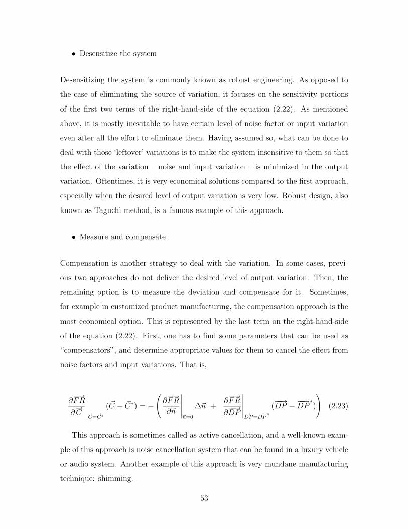
• Desensitize the system

Desensitizing the system is commonly known as robust engineering. As opposed to

the case of eliminating the source of variation, it focuses on the sensitivity portions

of the first two terms of the right-hand-side of the equation (2.22). As mentioned

above, it is mostly inevitable to have certain level of noise factor or input variation

even after all the effort to eliminate them. Having assumed so, what can be done to

deal with those ‘leftover’ variations is to make the system insensitive to them so that

the effect of the variation – noise and input variation – is minimized in the output

variation. Oftentimes, it is very economical solutions compared to the first approach,

especially when the desired level of output variation is very low. Robust design, also

known as Taguchi method, is a famous example of this approach.

• Measure and compensate

Compensation is another strategy to deal with the variation. In some cases, previ-

ous two approaches do not deliver the desired level of output variation. Then, the

remaining option is to measure the deviation and compensate for it. Sometimes,

for example in customized product manufacturing, the compensation approach is the

most economical option. This is represented by the last term on the right-hand-side

of the equation (2.22). First, one has to find some parameters that can be used as

“compensators”, and determine appropriate values for them to cancel the effect from

noise factors and input variations. That is,

∂−→FR

∂−→C

∣

∣

∣

∣

∣

∣

~C= ~C∗

( ~C − ~C∗) = −

∂−→FR

∂~n

∣

∣

∣

∣

∣

∣

~n=0

∆~n +∂−→FR

∂−−→DP

∣

∣

∣

∣

∣

∣

~DP= ~DP∗

(−−→DP −

−−→DP

∗)

(2.23)

This approach is sometimes called as active cancellation, and a well-known exam-

ple of this approach is noise cancellation system that can be found in a luxury vehicle

or audio system. Another example of this approach is very mundane manufacturing

technique: shimming.

53

2.2 Imaginary Complexity

In section 2.1, the uncertainty caused by the random nature of a system was dis-

cussed. It is represented by the probability of success of a set of desired functional

requirements, and this type of uncertainty is defined as a real complexity. The second

type of time-independent complexity in axiomatic design theory, imaginary complex-

ity, is defined as uncertainty that arises because of the designer’s lack of knowledge

and understanding of a specific design itself.

2.2.1 Ignorance in Design Process

Since the definition of imaginary complexity is centered on ‘ignorance’, which is quite

an ambiguous concept, it is necessary to explain what it really is. Recall that in

axiomatic design theory, a design is represented by a hierarchy of {FR}, {DP} and

[DM] as shown in figure 1-3. Thereby, ignorance, or lack of understanding can come

from these three sources.

Ignorance of {FR} is related to the failure to properly understand and define a

design task. For example, missing some of the essential functional requirements or

misinterpreting them, yields incomplete design as it addresses simply wrong problem.

Resulting design does not deliver truly desired functional requirements. While cap-

turing all of the essential functional requirements is critical, it should be noted that

having unnecessary functional requirements is not desirable as well since a larger set

of functional requirements tend to increase the uncertainty. To capture the functional

requirements no more and no less than necessary can be very challenging task. It is

particularly so when sociological/psychological factors are considered: for example,

in many consumer electronics, technologically unnecessary - or rarely appreciated -

functions can be added for marketing purpose. Missing some of those technically-

inessential functional requirements may lead to disastrous business consequence. The

importance of selecting the best set of functional requirements cannot be overempha-

sized. Specifying excessively tight design range is another type of ignorance of {FR}.

Obviously, that will make the design problem more challenging than it should be.

54

One can make any design problem arbitrarily difficult by requiring that its output be

infinitely precise. Therefore, it is crucial to know appropriate level of design range

for functional requirements. Unfortunately, the problem of assessing the right level of

design range throughout the system hierarchy has not been clearly understood yet,

which is part of the reason why tighter specification is common in practice. Overall,

ignorance of {FR} increases uncertainty of a system above what it really is, and thus

contributes to imaginary complexity.

Lack of knowledge required to synthesize or identify proper {DP} will increase the

uncertainty. This type of ignorance can be due to the sheer absence of technological

expertise in a particular subject matter or inability to predict emergent effect when

a particular solution is implemented. Oftentimes, advances in technology resolve the

problem. On the other hand, as seen from the planet motion example in section 1.1, it

could be due to wrong choice of model to solve the problem. The uncertainty caused

by the above is not inevitable, and thus imaginary.

Yet, these types of ignorance are very difficult to effectively measure because

the context of such ignorance is in the semantic domain. Therefore, even though

we can qualitatively argue that the uncertainty is the consequence of the lack of

knowledge on the subject matter, any degree of quantification seems formidable as

of now. However, the uncertainty caused by these types of ignorance is still part of

imaginary complexity in a qualitative sense. For the sake of quantification, complexity

discussion in axiomatic design theory limits the scope of the term to the ignorance of

the [DM] structure [2]. It focuses on the iteration in the design process, and comes

up with a particular measure for it.

2.2.2 Iteration in Design Process and Imaginary Complexity

Almost inevitably, design process involves some iterations. Iteration in design pro-

cess may have different meanings depending on the context, and here, it strictly

refers to the iteration to reach a set of target values of responses through successively

changing values of a set of inputs. Iteration process - number of iterations, sequence,

convergence, etc. - is dictated by the interrelationship among the inputs and target

55

responses. In axiomatic design framework, design parameters and functional require-

ments correspond to inputs and target responses respectively, and a design matrix is

used to represent the interrelationship among the FRs and DPs. For uncoupled de-

sign, which has a diagonal design matrix, DPs and FRs have one-to-one relationship,

and thus it does not require any iteration in getting each of the functional require-

ments on target value. For decoupled design, some of DPs affect more than one FRs

with one-to-many relationships. As a consequence, there exists a certain sequence

only through which target values for FRs can be reached without iteration. In case of

a coupled design, the desired FR values are obtained through a number of iterations.

In the attempt to satisfy all the desired functional requirements, one has to follow

a certain sequence dictated by the structure of the design matrix, if there exists such

sequence. Failure to do so will cause unnecessary iterations or even non-convergence

as shown in Figure 2-4, which eventually increases the uncertainty in achieving the de-

sired functional requirements. Therefore, it is important to understand the structure

of design matrix to avoid undesirable consequence. Based on the above reasoning,

the probability of selecting a correct sequence is associated with the uncertainty in

achieving functional requirements. The imaginary complexity is defined as following:

CI = log21

p(selecting a correct sequence)(2.24)

FRi

FRj

DPb

DPa

FR*j

FR*i?? FRi

FRj

DPb

DPa

FR*j

FR*i

(a) (b)

FRi

FRj

DPb

DPa

FR*j

FR*i?? FRi

FRj

DPb

DPa

FR*j

FR*i

FRi

FRj

DPb

DPa

FR*j

FR*i??

FRi

FRj

DPb

DPa

FR*j

FR*i?? FRi

FRj

DPb

DPa

FR*j

FR*i

FRi

FRj

DPb

DPa

FR*j

FR*i

(a) (b)

Figure 2-4: Design iteration can be non-converging by (a) selecting inappropriate DPfor FR or (b) singularity

For uncoupled design, p(selecting a correct sequence) is 1 since any arbitrary

56

sequence is valid. Iteration is not needed, which means no uncertainty associated

with additional iteration. Thus, CI is 0. For a coupled design, the probability is

not defined because there exists no right sequence in coupled design. In a decoupled

design, the probability is (z/n!) where z is the number of valid sequences and n is

the total number of functional requirements.

It is interesting to note that the probability is not a function of the size of design

matrix. It is rather a function of the precedence relationships among FRs and DPs,

which is roughly the number of off-diagonal elements in the matrix. For example, a

2×2 decoupled design has the same probability as a 7×7 matrix with one off-diagonal

element. For 2×2 decoupled matrix, z is 1 and n is two. Thus, the probability of

selecting the correct sequence is

p = 1/2! = 0.5 (2.25)

For 7×7 matrix with one off-diagonal element, there is only one precedence re-

lationship as in 2×2 case. Therefore, the probability should be also 0.5. z is

5!×(6C2 + 1), and n is 7. The probability is

p =

5!×

6

2

+ 6

7!(2.26)

= 0.5

which agrees with our intuition.

The definition of CI has some problems. First of all, strictly equating the probabil-

ity of finding a correct sequence to the probability of success is a bit of overstatement.

Selecting wrong initial sequence does not exclude the possibility of reaching a solu-

tion. It is very possible that the solution can be obtained through some iteration even

when the initial sequence tried is not the correct one. Also, the probability of (z/n!)

assumes completely random trial when changing DP values to satisfy functional re-

57

quirements, which is rarely the case in practice. Therefore, it is rather a lower bound

– worst case – in the presence of decoupled elements. The fact that it is only appli-

cable to decoupled design also weakens the utility of the concept. More fundamental

problem is, though, that the quantity CI carries little practical meaning because once

we are able to measure CI , it is not there anymore: measuring CI requires knowledge

about the structure of design matrix, which will, in turn, eliminate CI .

In spite of some controversial aspects in its metric, CI , the concept of imaginary

complexity is still valid in a pedagogic sense. It is very acceptable that failure to

recognize the structure of design matrix, i.e. interactions among FRs and DPs, will

cause some uncertainty even when the design solution is indeed good. That is clearly

undesirable and must be avoided. Therefore, the main message that needs to be em-

phasized regarding the imaginary complexity is “in order to minimize the uncertainty

in achieving functional requirements, one has to know what (s)he is doing before

doing it.”

2.3 Information Content vs. Complexity

Having followed the discussion on real complexity (and imaginary complexity), one

might suspect that the concept of complexity is not different from the information

content: complexity is defined as a measure of uncertainty, and the information con-

tent is defined in terms of probability of success for a functional requirement(s) that

is, in fact, uncertainty.

Let us revisit the definition of complexity in axiomatic design. Complexity is

a certain quality or quantity, perceived in regard to a designed system, that is a

consequence of the uncertainty in achieving a desired set of functional requirements.

Thus, strictly speaking, complexity is not the same as uncertainty. Since it is such an

abstract concept, there is no direct measure for it. In search of a metric, it is forced to

consider a reasonable surrogate. By hypothesizing that complexity is proportional to

the uncertainty in achieving functional requirements, the uncertainty itself is chosen

as a measure of complexity. Therefore, uncertainty is a measure of complexity, and

58

at the same time, complexity is a measure of uncertainty.

Generally, uncertainty is directly related to probability, and it is true that prob-

ability is a good metric for uncertainty. However, uncertainty in axiomatic design

can be understood in a probabilistic context and a non-probabilistic context. In

probabilistic sense, the uncertainty is related to the probability of success ps. Zero

probability gives infinite uncertainty, and probability of one yields zero uncertainty.

By the probabilistic nature of the concept, this type of uncertainty has its cause in

the randomness around a design, i.e. DP variation, noise, etc. Naturally, this type

of uncertainty is measured directly by information content, I = log21/ps. In non-

probabilistic context, the uncertainty cannot be easily quantified by probability. The

uncertainty in this context is improbability or un-likelihood that can be attributed to

non-probabilistic factors such as ignorance. In spite of the lack of quantitative mea-

sure, the existence of this type of uncertainty is out of doubt. Information content,

while a reasonable measure for uncertainty in probabilistic context, cannot extend

further to reach non-probabilistic regime of uncertainty. That is the main reason to

introduce the concept of complexity.

Imaginary complexity would not have been realized if we had focused only on

information content, and neither would time-dependent complexity concept. The

contribution of complexity concept is that it enables to investigate the subject of

uncertainty in various dimensions in addition to probabilistic perspective.

2.4 Summary

Time-independent complexity is the complexity where uncertainty in achieving func-

tional requirement is time-independent. It implies that its system range does not

change over time and that functional requirements are also time-independent. Two

types of time-independent complexity is defined in axiomatic design theory: real

complexity and imaginary complexity.

Real complexity accounts for random nature of a system, and is defined as a

measure of uncertainty when the probability of achieving the functional requirements

59

is less than 1 because the common range is not identical to the system range. By its

definition, it is equivalent to information content since information content measures

the uncertainty in the same probability context. Information content is defined as a

function of probability of success. Estimating probability of success typically requires

simulations or experiments, but if design equations are known and simple, it can be

easily derived. Information content is almost same as Shannon information, but two

concepts are subtly different because of the way information is interpreted.

Reducing real complexity is essentially reducing variation in functional require-

ments. Common engineering research and practice include 1)eliminating source of

variation, 2)desensitizing a system, and 3)compensating for the variation. Based on

technical and economic consideration, these three approaches must be combined for

optimal result.

Imaginary complexity, on the other hand, accounts for the uncertainty due to ig-

norance. Lack of proper understanding of functional requirements, lack of knowledge

or wrong choice of design parameters, and ignorance of design matrix structure in-

crease the uncertainty. Even though the ignorance is difficult to effectively measure,

the existence and its effect on uncertainty is out of doubt. Quantitative definition of

imaginary complexity in axiomatic design is limited and imperfect, but the message

is still valid.

60

Chapter 3

Time-dependent Complexity

As opposed to time-independent complexity, time-dependent complexity requires time

dimension as one of its determinants. Although it may not be an explicit function

of time, the behavior of functional requirements necessitates time factor for proper

description of it. According to Suh’s definition [2],[24], for time-dependent complexity,

the uncertainty changes as a function of time. Why would the uncertainty change

over time? The time-dependency can come from either 1) time-varying system range

or 2) unpredictability of functional requirements in future.

Time-dependent complexity is divided into two different kinds: combinatorial

complexity and periodic complexity. In a combinatorial complexity case, the uncer-

tainty grows indefinitely whereas it stops increasing and returns to the initial state

occasionally in case of periodic complexity. In some sense, a system with a com-

binatorial complexity behaves in a similar way as a chaos system does. Chaos, or

sometimes simply called a dynamic instability, is defined as the extreme sensitivity

to the initial condition. Two nearly indistinguishable initial conditions would result

in two final predictions which differ vastly from each other.

One of the most interesting issues in the study of time-dependent complexity sys-

tem is whether or not the presence of combinatorial complexity leads to unmanageable

design task and, if it does, whether or not it can be reduced to certain degree.

In this chapter, the origin of time-dependency is discussed: time-varying system

range and unpredictability of functional requirements in future. Then, functional

61

periodicity is introduced to define the concept of periodicity, semi-periodicity, and

aperiodicity. This discussion will serve as the theoretical basis for the work presented

in the remaining of this thesis.

3.1 Time-dependent Complexity

By Suh’s original definition, complexity is a measure of uncertainty in achieving a

desired set of functional requirements. This definition implies that the complexity is a

consequence of being uncertain about delivering required FRs or that the uncertainty

is a symptom of a system’s being complex. In section 2.3, it is argued that complex-

ity is a measure of uncertainty and at the same time, the uncertainty is a measure

of complexity. It is particularly explicit for time-independent real complexity: com-

plexity is measured by the information content, which measures the (probabilistic)

uncertainty. Either way, it is clear that time-dependency of complexity is related to

time-dependency of uncertainty. In other words, for time-dependent complexity, the

uncertainty changes as a function of time. So, if it changes with time, the direction

of change is going to be of our concern. If it decreases, then it is less of a problem.

For such case, major attention will be given to the initial uncertainty and the rate

at which it decreases. One example of such systems is a speech recognition system

with learning capability. The uncertainty in performing a given task, recognizing

natural spoken language, becomes smaller and smaller with time1. Unfortunately,

there are much more instances where the uncertainty increases with time. Systems

with dynamic instability, which many real world systems are considered as, present

increasing uncertainty. In a mechanical system, wear of its components typically in-

creases uncertainty in its functionality. This ever-increasing complexity can possibly

pose serious problems such as sustainability and stability. It is this increasing un-

certainty that axiomatic design’s time-dependent complexity discussion has its focus

on.

1Performance of such system improves as it processes more and more reference data. It is assumedthat the amount of data it processes is proportional to the time of its operation.

62

Recall that there are two types of uncertainty: quantitative (quantifiable) and

qualitative (non-quantifiable). The first type of uncertainty is subject to probabilistic

treatment, and thus is related to time-varying system range. The second type is

explained in terms of the unpredictability of functional requirements in future.

3.1.1 Time-varying System Range

Time varying system range is illustrated in figure 3-1 for a simple single-FR case.

Given a design range, suppose that a design solution initially yields a system range

indicated by a solid line. For a variety of reasons, after a certain time period, the

system range can change and deviate from its initial distribution as indicated by

dotted lines, thereby changing the probability of success. The new probability of

success at time t is,

pts =

∫

design

range

f t(FR)dFR (3.1)

Since FR is a function of design matrix and design parameter, this change can be

due to the shift in the mean of design parameter, increased variation of design param-

eter, and/or change in design matrix element. Uncoupled n-FR design is equivalent

to n single-FR problems and thus treated similarly as a single-FR case. The overall

probability of success is simply the product of the individual probability of success

for n FRs.

For decoupled and coupled n-FR design, change in any one of the FRs always

implies resulting change in the joint probability density of n FRs as well as its own

marginal probability. That is also the case with uncoupled design, but there is one

obvious but important difference. Unlike uncoupled design, the change in one FR in a

decoupled/coupled design may be associated with other FR’s distribution depending

on the structure of design matrix. For example in a hypothetical design of equation

(3.2), change in DP1 affects both FR1 and FR2 distributions whereas change in DP2

results only in FR2 distribution. This should be obvious once the design matrix

structure is understood.

63

FRdru

p.d.f.f(FR)

drl

System Range at time t0,f(FR, t0)

Design Range |dr|

t

FRdru

p.d.f.f(FR)

drl


Design Range |dr|

t

Figure 3-1: Time-varying system range for a single FR

Time-varying system range for multiple FR

Less obvious is the fact that monitoring individual marginal probability could be

quite misleading in making decisions regarding the change of system range. Even

though the FRs being monitored individually seem well under control, the overall

probability of success could be decreasing. In chapter 2, it was shown that correct

computation of probability of success for multi-FR, unless uncoupled, requires joint

probability density function be evaluated rather than marginal probability density

function. It has to be emphasized again that all of the relevant functional require-

ments have to be considered simultaneously, i.e. one must pay attention to the joint

probability rather than marginal probability. Consider, for example, the following

2-FR decoupled design.

FR1

FR2

=

1 0

1 1

DP1

DP2

(3.2)

For the sake of simplicity, assume that DP1 and DP2 initially follow uniform

distributions U[-1,1] and U[0,1.5] respectively. The joint probability density function

for (FR1, FR2) is a uniform probability of 13over the range shown in figure 3-2(a).

Marginal probability density functions for FR1 and FR2 are shown in figure 3-2(b)

64

p.d.fFR1

FR2

-1

-1 1

1.5

-1

0.5

FR2

FR1

p.d.f

-1 1

0.5

0.5

(a) (b)

(c)

2

-2Design range

Joint p.d.f.(FR1,FR2)

2.5 2.5

1

p.d.fFR1

FR2

-1

-1 1

1.5

-1

0.5

FR2

FR1

p.d.f

-1 1

0.5

0.5

(a) (b)

(c)

2

-2Design range


2.5 2.5

1

Figure 3-2: (a) Joint p.d.f. of (FR1, FR2) is defined over the parallelograms, (b)marginal p.d.f. of FR2, and (c) marginal p.d.f. of FR1

and (c) respectively. Suppose that p.d.f. of DP2, after some time t, has been changed

to U[-1,1.6]. Then, the joint probability density of (FR1, FR2) changes accordingly

as shown in figure 3-3(a). The value of new p.d.f. is p = 15.2

, and the parallelogram

is also changed. Note that the marginal probability density function for FR1 still

remains same for both cases: U[-1,1]. Therefore, until the change in FR2 or the joint

distribution of (FR1,FR2) is monitored, the overall system’s deterioration is hidden.

Monitoring the marginal distribution of FR2 will resolve the problem only partially:

it could lead to a wrong conclusion about the system’s performance. Suppose the

design range for FR1 and FR2 is [-0.5,0.5] and [-2,2] respectively. This design range

corresponds to a rectangle on FR1-FR2 plane as shown in figure 3-2 and 3-3. Table

3.1 summarizes the probability calculation for the system before and after the change.

As you can see, the marginal probability for FR1 remains same at 0.5 after the change,

and it even slightly increases by 0.007 for FR2. Given such information, it is likely to

conclude that the system is producing better output. On the contrary, however, the

overall probability of success, i.e. the probability determined by joint distribution,

shows slight decrease from 0.5 to 0.499. This example shows the effect of statistical

65

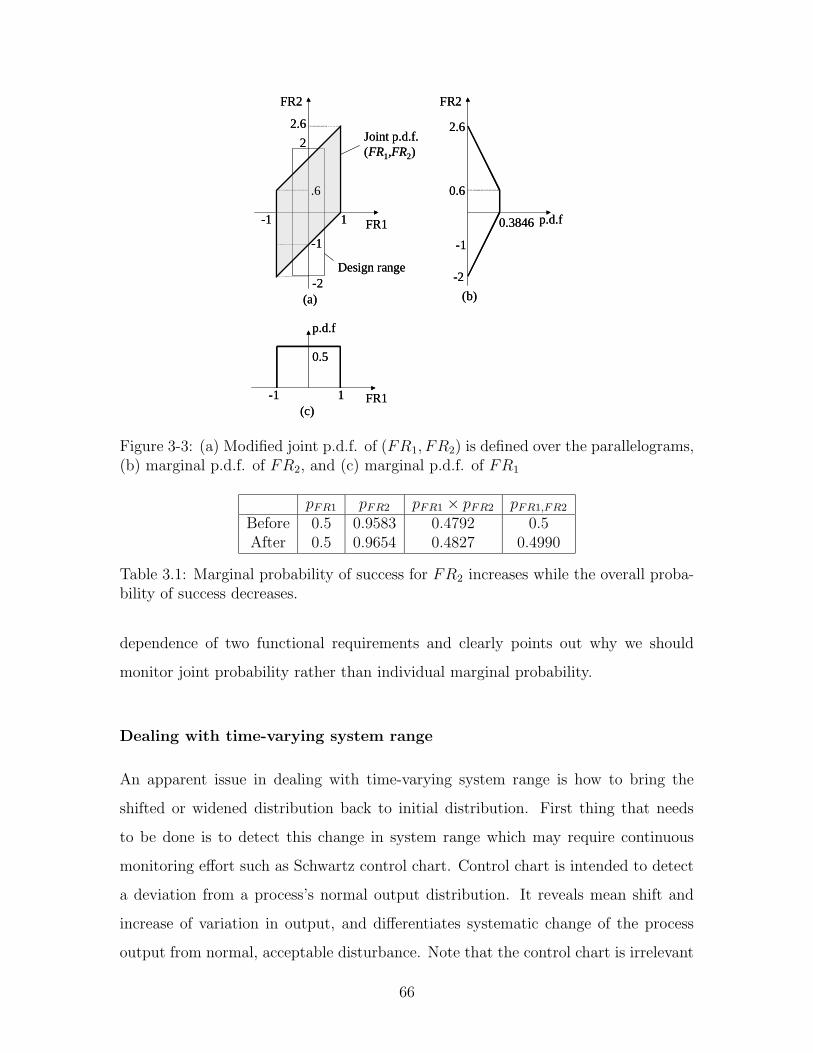
p.d.fFR1

FR2

-1

-1 1

-1

0.3846

FR2

FR1

p.d.f

-1 1

0.5

0.6

(a) (b)

(c)

2

-2Design range


2.6 2.6

.6

-2

p.d.fFR1

FR2

-1

-1 1

-1

0.3846

FR2

FR1

p.d.f

-1 1

0.5

0.6

(a) (b)

(c)

2

-2Design range


2.6 2.6

.6

-2

Figure 3-3: (a) Modified joint p.d.f. of (FR1, FR2) is defined over the parallelograms,(b) marginal p.d.f. of FR2, and (c) marginal p.d.f. of FR1

pFR1 pFR2 pFR1 × pFR2 pFR1,FR2

Before 0.5 0.9583 0.4792 0.5After 0.5 0.9654 0.4827 0.4990

Table 3.1: Marginal probability of success for FR2 increases while the overall proba-bility of success decreases.

dependence of two functional requirements and clearly points out why we should

monitor joint probability rather than individual marginal probability.

Dealing with time-varying system range

An apparent issue in dealing with time-varying system range is how to bring the

shifted or widened distribution back to initial distribution. First thing that needs

to be done is to detect this change in system range which may require continuous

monitoring effort such as Schwartz control chart. Control chart is intended to detect

a deviation from a process’s normal output distribution. It reveals mean shift and

increase of variation in output, and differentiates systematic change of the process

output from normal, acceptable disturbance. Note that the control chart is irrelevant

66

Figure 3-4: Cause-and-effect diagram

of design range. To be more useful, the information from control chart should be

used along with design range because it puts the information in the proper context.

As discussed above, for more than one FR case, unless the system is uncoupled,

functional requirements have to be monitored jointly, i.e. its joint distribution must

be monitored rather than individual marginal distribution.

Once deterioration from the original distribution is discovered, assignable causes

must be identified. A cause-and-effect diagram2(figure 3-4) is an example of common

practices to find root causes of the problem. Methods like Schwartz control chart and

cause-and-effect diagram are commonly termed as statistical process/quality control

(SPC/SQC). A complete decomposition of functional requirements and design pa-

rameters along with associated design matrix should be very helpful when identifying

the root cause of the problem. One of the reasons why it is typically hard to find out

the root cause is that they attempt to link directly between a symptom (high-level

FR) and low-level parameters. If the architecture of the system is well understood

and represented by {FR}-[DM]-{DP} hierarchy, it quickly narrows down the scope

of the problem of locating the root cause [25]. Indeed, the flow-diagram represen-

tation of system architecture in axiomatic design can be used as the platform of a

cause-and-effect diagram.

We know some of the common causes of varying system range always exist in

reality. Examples are tool wear, machine component wear, fatigue, etc. To avoid the

cost of system range deterioration, which could sometimes be significant, preventive

2It is interchangeably called ’fishbone diagram’ or ’Ishikawa diagram.’

67

maintenance can be carried out instead of waiting until the change has happened due

to the common causes. Obviously, frequency of preventive maintenance and the cost

associated with it must be traded off against the cost of losing process capability.

Although sometimes it may be the only option in practice, SPC approach to

recover original system range is not a fundamental solution to the problem. Funda-

mental solution that must be sought for whenever and wherever feasible is to make

a design more robust and reliable as much as possible. Following example illustrates

how a design change effectively delays the system range deterioration.

Example 3-1: Decoupling a Knob Design

Let us consider the “Knob design” example presented in [2]. It has to

satisfy two functional requirements:

FR1 = Grasp the end of the shaft tightly

FR2 = Turn the shaft

DPs are chosen such that the two FRs are satisfied. Refer to figure 3-5

for illustration:

DP1 = Interference fit (between the shaft and the inside diameter of the

knob)

DP2 = Flat surface

Design (a), one of the implementation of the above DPs, is a decoupled

design3 : when the torque is applied by the knob, the grip force on the

shaft decreases with the increase of the slot opening as a result of normal

load acting on the flat surface. As a result of coupling in design (a), the

knob will slide off the shaft after certain period of use. In other words,

FR1, grasping force, is getting out of design range as time elapses. One

way of dealing with this problem is to simply increase the wall thickness

3In [2], design matrix element (2,1) is said to have a small value, and accordingly the design wasconsidered ’weakly-coupled’. For the sake of our discussion, it can be ignored because the problemoccurs due to the dependence of FR1 from FR2 - design matrix element (1,2).

68

of the knob. It will increase the stiffness of the knob such that it has

bigger resistance to slot opening, and thus will sustain longer period of

use. However, it induces another problem: to make the interference fit

work without excessive force requirement in manufacturing process, a tight

control over the part dimensions must be maintained. This will bring up

the process control issue, and likely incur additional cost in manufacturing.

More fundamental approach is to get rid of the root cause, which is, in

this case, the dependency of FR1 on the FR2. Such a design is presented

in (b). In this design, the slot terminates where the flat part of the knob

begins. Because the flat surface is completely away from the slot, the

turning action does not force the slot to open and, therefore, the axial

grip is not affected. Achieving an uncoupled design by the slight design

change delays the system range deterioration.

��

��

�� ! �� "� � ��"� � # ��

$��

%

%

$�� &� � ��' � ��()%*%

+ � ,

+ ��,

�� ! �� "� � # � ��

(a) (b)

��

��

�� ! �� "� � ��"� � # ��

$��

%

%

$�� &� � ��' � ��()%*%

+ � ,

+ ��,

�� ! �� "� � # � ��

(a) (b)

Figure 3-5: Knob design example (adapted from [2])

3.1.2 Unpredictability of Functional Requirements in Future

Previous section discusses the time-dependent complexity caused by time-varying sys-

tem range. It implicitly assumes that functional requirements and their design ranges

are static. The second type of the source of time-dependency is the unpredictability of

FRs in future. This unpredictability is related to time-varying attribute of functional

69

tfinish t

T

Tini

tstart t

TTini

tfinishtstart

T*(t)T**(t)

(a) (b)

tfinish t

T

Tini

tstart t

TTini

tfinishtstart

T*(t)T**(t)

(a) (b)

Figure 3-6: Desired FR values are changing as a function of time, and thus dynamicFR. From design perspective, however, T*(t) is not different from T**(t).

requirements. The complexity in axiomatic design can only be defined in relation with

functional requirements, and thus the functional requirements’ dependence on time

makes associated complexity also dependent on time. It is possible that, even without

time-varying system range, there is time-dependence due to functional requirements.

There can be different types of time-varying behavior of functional requirements.

Functional requirements are considered time-dependent when 1) target FR values

are time-varying and 2) the elements of a set, {FR}, changes. The former was called

dynamic FR [26], and the latter was discussed by Suh[27] when defining large system.

Following example illustrates the concept of dynamic FR.

• FR: Control temperature profile of a heating chamber

This FR can be re-stated as “T = T ∗(t) while tstart ≤ t ≤ tfinish ”, and shown

in figure 3-6. As you can see, the functional requirement is surrogated by a specific

variable, i.e. T in this example, and the target value of it is varying as a function

of time. A sophisticated version of this FR can be found in photoresist processing

system in semiconductor manufacturing, and a mundane example would be a toaster

oven in your kitchen. Once the function is initiated, its target value is moving along

a specified trajectory as a function of time. It is obviously time-dependent in view of

its operation – FR value is changing over time –, but if we consider designing process,

time factor is not particular concern for this type of FR. For example, designing for

a trajectory T ∗ is not different from designing for T ∗∗ in figure 3-6. Also, time t is

not critical factor in a sense that achieving the FR - T (t) = T ∗(t) - at any time t1

is not necessarily more uncertain than achieving the FR at other time t2. If it does,

70

FUNCTIONALREQUIREMENT

DESIGN PARAMETER

Input:Target trajectory

tfinish t

T

Tini

tstart

T*(t)


tfinish t

T

Tini

tstart

T(t)

Output:Actual trajectory

Follow/Control temperature

FUNCTIONALREQUIREMENT

DESIGN PARAMETER


tfinish t

T

Tini

tstart

T*(t)

tfinish t

T

Tini

tstart

T*(t)


tfinish t

T

Tini

tstart

T(t)

Output:Actual trajectory

Follow/Control temperature

Figure 3-7: A representation that separates design process and operational signalflow. Time-dependence is now part of the input instead of FR.

it is more likely due to the value T than t. When the uncertainty does increase as

t increases, then this problem becomes the same type as time-varying system range

problem. The main concern of design is to come up with design parameter(s) to cover

the entire operating range, [T l, T u], with required error level, ε = T (t) − T ∗(t). It

is most likely that this functional requirement is accompanied by static (constant)

design range, which makes this type of problem less time-dependent. Therefore, even

though the functional requirement value is time-varying in operation, its design is

more like a static functional requirement from design perspective in a sense that we

deal with the same functional requirement – that FR happens to be two dimensional –

all the time. It can be shown more clearly if we take slightly different representation

of FR-DP with operational input and output concept. In representation shown in

figure 3-7, functional requirement is “Follow/Control temperature within the range

[T l, T u] with error level ε ≤ ε∗.” While the functional requirement is semantically

stated, the diagram representation treats the FR box as a kind of transfer function.

It takes the input, which is temperature trajectory, and the functional requirement

is achieved to produce actual output trajectory. Design parameter that can achieve

this function is shown in the box beneath the FR box. So, FR-DP mapping is

represented vertically, while the signal4 flows horizontally. Thereby, design for this

functional requirement - vertical interaction - is separated from time-dependent aspect

of operational input/output, and thus time-independent.

4It can also be material or energy.

71

The other type of time-dependency of FR arises when the elements of a set,

FR, changes as a function of time. It is meaningful only when multiple number

of functional requirements exist. Functional requirements are time-dependent in a

sense that they are relevant at certain time (or duration), and become irrelevant

at other time. For example, suppose a set FR consists of seven member FRs, i.e.

FR = {FRa, FRb, FRc, FRd, FRe, FRf , FRg}. At different times, different subset

of FR needs to be satisfied. That is,

t = t1 FR = {FRb, FRc, FRd, FRg}

t = t2 FR = {FRa, FRe}...

...

At a particular time, FR consists of different combinations of FRs, signifying

time – or sequence – as an important factor. In this case, one of the immediate issue

is to avoid coupling at every ti. First of all, number of available DP s must be no fewer

than number of FRs at any time. Theorem 1 in axiomatic design states that “when

the number of DPs is less than the number of FRs, either a coupled design results or

the FRs cannot be satisfied.” The theorem is modified to include this time-dependent

characteristics:

Theorem 1′: When the number of DPs is less than the number of active

FRs at any given time, either a coupled design results or the FRs cannot

be satisfied for the duration.

While we want enough number of DP s as a necessary condition to satisfy functional

requirements, it is not desirable either to have too many DP s. Having more than

necessary DP s results in redundant design and potentially inefficient design. By the

fact that not all FRs are active at the same time, it may be possible to use some

of DP s to satisfy multiple FRs without causing coupling. Using the same DP for

more than one functional requirement is sometimes called ‘function-sharing.’ By the

modified theorem 1, each FR’s belonging to different subset FR is the necessary

condition for successful function-sharing. In order to maintain optimal number of

DP s – neither fewer nor more than number of FR at any given time –, prediction

72

of FR(t) is necessary. If a system’s FR is unpredictable, it is difficult to achieve

the goal. Therefore, the predictability of FR(t) becomes important in a system with

time-dependent FR.

Time-dependency of FR implies that the functional requirements are recurring.

The recurrence of functional requirements brings up a couple of issues which have not

been considered for time-independent complexity. As discussed above, predictability

of the pattern of FR(t)is an important factor. Recurrence of FRs naturally relates

to periodicity of FR. In some cases, periodicity, which is defined in section 3.2, may

be necessary condition for a system to sustain its functionality without becoming

chaotic. Sometimes, sequence of functional requirements’ occurrence is of a concern.

Identifying correct precedence relationships between FRs and mechanism to ensure

such precedence relationships are among the important design tasks. Triggering and

stopping each of FRs at right moment is required. Completeness of FR is also an

essential problem. All FRs must be achieved when they become present. In some

cases, they have to be achieved once and only once (or twice and only twice, etc.)

within a certain period. The completeness of recurrence of FRs naturally relates to

periodicity of FR, and it is indeed the basis for defining periodicity.

Time-dependency of FR

In this section, ui, the binary random variable that was defined in section 2.1.2, is

revisited to represent time-dependency of functional requirements and periodicity.

Recall ui for time-independent functional requirements. ui for FRi, was defined as

following:

ui =

1 with pi

0 with 1− pi

(3.3)

The information content is, then, written as

I(ui = 1) = −log2(pi) (3.4)

73

If we consider ui as a state variable, then for multiple number of functional require-

ments, a state vector u, can be defined:

u = {u1, u2, . . . , uN} (3.5)

For time-independent case, the concerns are what is the probability of u = {1, 1, . . . , 1}

and how to increase the probability.

For time-dependent case, functional requirements are time-dependent in a sense

that they are present or absent at particular time period. The definition of ui is

modified to include time factor:

ui(t) =

ui for t ≥ τi

0 for t < τi

(3.6)

where, τi is the time when FRi emerges (or is decided whether achieved or not

achieved). This definition basically accounts for the fact that an FR does not exist

prior to certain time, t, which is peculiar to time-dependent FRs.

Then, the FR state vector, u becomes

u(t) = {u1(t), u2(t), . . . , uN (t)} (3.7)

By definition of ui(t), u(0) = {0, 0, . . . , 0} and after certain time T, when all the func-

tional requirements are achieved, u(T ) = {1, 1, . . . , 1}. Note that time-dependency

implies that functional requirements are recurring, i.e. they appear repeatedly and

need to be achieved every time. Otherwise, introducing time factor may have not

been necessary. Recurrence of functional requirements requires the issues such as

periodicity be resolved.

A set of functional requirements is said to be deterministic if all of τi are known

a priori. In such a deterministic set of functional requirements, u(t) is evidently a

function of time. For example, assume, 0 < τ1 < τ2 < τ3 < . . . < τN .

u(0 < t < τ1) = {0, 0, . . . , 0}

74

u(τ1 < t < τ2) = {u1, 0, . . . , 0}

u(τ2 < t < τ3) = {u1, u2, 0, . . . , 0}

u(τN < t) = {u1, u2, . . . , uN}

Given that time-dependent FR implies recurrence, it is obvious that if τi is constant

for all i, then the system is periodic.

Now that u(t) is defined, we can define probability of success for time-dependent

situation. Since ui(t < τi) is zero by definition, if we simply define the probability

of success as in time-independent case, it is always zero until t > τN . Therefore,

we need to introduce a modified version of the probability of success. In doing so,

it seems reasonable to define “success” at any given moment as achievement of the

ideal state at that moment, ideal state being a state where all the present functional

requirements are achieved. Then, probability of success becomes the probability of

u(t) = u∗(t), where * indicate the ideal state. That is,

ps(t) = p[u(t) = u∗(t)] (3.8)

For example, in the deterministic case,

u(τ2 < t < τ3)∗ = {1, 1, 0, . . . , 0}

u(τ2 < t < τ3) = {u1, u2, 0, . . . , 0}(3.9)

The probability of success at time τ2 < t < τ3, ps(τ2 < t < τ3) is p(u1 = 1, u2 =

1, 0 = 0, . . .). Since {0=0} is redundant, ps(τ2 < t < τ3) is p(u1 = 1, u2 = 1). That

is the joint probability of both FR1 and FR2 being achieved. ps(t < τ1) is 1 since

u(t) = 0 and u(t)∗ = 0. ps(t > τN) is p(u1 = 1, u2 = 1, . . . , uN = 1), which is the

probability of all FRs’ being achieved. The probability of success, as defined above, is

time-dependent, and that is one of the characteristics of time-dependent complexity.

75

3.2 Functional Periodicity

Having identified two different kinds of time-dependency – time-varying system range

and time-dependent {FR} –, this section introduces the concept of periodicity. In

axiomatic design, time-dependent complexity is divided into two different kinds: pe-

riodic complexity and combinatorial complexity. Criteria for differentiating the two

time-dependent complexity is the existence of periodicity.

First, the apparent periodicity can be defined by system range’s behavior. As

shown in figure 3-1, time-varying system range changes and deviates from its initial

desired distribution, decreasing probability of success. A system is said to have a

periodicity, and thus periodic complexity, if the system range regains its initial state

periodically (see figure 3-8). It should be noted that the periodicity is not defined in

terms of time as opposed to conventional perception of periodicity. The periodicity

in axiomatic design complexity discussion does not require regular interval – period

– as part of its definition. Definition of periodicity is based purely on the ability to

regain the initial state. When the system range retrieves its initial state, it is said to

be reinitialized. For this to happen, either internal of external action has to be taken,

and such action is called reinitialization.

Secondly, periodicity can be defined based on the time-dependency of functional

requirements. In the previous section, time-dependency of FR was represented by

time-varying set of {FR}, u(t). Here, u(t) is used again to define periodicity, partic-

ularly functional periodicity. Depending on its pattern of appearance, three different

types of functional periodicity can be defined: semi-periodic, periodic, and aperiodic.

Periodic There exist Ti such that u(0) = u(T1) = u(T2) = · · · with regular transition

pattern

Semi-periodic There exist Ti such that u(0) = u(T1) = u(T2) = · · · without regular

transition pattern

Aperiodic None of the above

If a system’s functional requirement set has the initial state where no FR is present

76

FRdru

p.d.f.f(FR)

drl


Design Range |dr|

t

f 0)

| |

Return to initial distribution

FRdru

p.d.f.f(FR)

drl


Design Range |dr|

t

f 0)

| |


Figure 3-8: System range regains its initial distribution after it has been degraded.A system with this characteristics is said to have periodicity.

and final state where all the FRs are accomplished once (or twice, thrice, etc.), and

they occur repeatedly, it is said to have semi-periodicity. If the pattern between the

initial state and final state is consistent, then it is periodic. If none of these conditions

are met, such system is said to be aperiodic. See figure 3-9 for illustration. Figure

3-9(a) represents periodic {FR}. A system begins with null state, u(0), and reaches

fully-active state, u(T − δ). Each of five FRs becomes active (relevant) in the same

sequence – FR1-FR4-FR3-FR2-FR5 – for every period. In semi-periodic case, the

system begins with null state and reaches fully-active state as with periodic case, but

the transitional pattern is different from one period to another: FR1-FR4-FR3-FR2-

FR5 for the first period, and FR5-FR2-FR3-FR1-FR4 for the next period. Still all

five FRs become active exactly once in a period. In that sense, the state at t = T1 is

not different from that of t = T2. Figure 3-9(c) shows no regularity at all, and thus

called aperiodic.

Aperiodic behavior is simply the behavior that occurs when no variable describing

the state of the system’s functional requirements undergoes a regular repetition of

values. Aperiodic behavior never repeats and it continues to manifest the effects of

any small perturbation; hence, any prediction of a future state in a given system that

77

u1

u0

u2

u3

u4

u5

t

FR S

tate

T1 T2

(a) Periodic

u1

u0

u2

u3

u4

u5

t

FR S

tate

(b) Semi-periodic

u

T1 T2

u1

u0

u2

u3

u4

u5

t

FR S

tate

(c) Aperiodic

u1

u0

u2

u3

u4

u5

t

FR S

tate

(c) Aperiodic

Figure 3-9: Illustration of Periodic/Semi-periodic/Aperiodic u(t)

is aperiodic is impossible unless it is completely deterministic.

It should be noted that the value Tk does not have to be a constant. The length

of the interval between null state to the next null state does not have to be a constant

value. This is equivalent to saying that we are interested only in the sequence and/or

completeness of {FR}, not in the actual time interval. Since we have not found

alternative terminology for proper name for it, we have no choice but to use the term,

periodicity. But, unlike conventional periodicity concept, the periodicity here does

not necessarily require regular interval as part of its definition. In other words, the

periodicity here means the functional periodicity rather than the temporal periodicity.

The length of period is indeed determined by the functional period.

Recall the probability of success for time-dependent case:

ps = p(u(t) = u(t)∗)

If it is either periodic or semi-periodic, we can say u(0) = 0 without loss of

generality. For periodic case, it is obvious. For semi-periodic case, since u(T1) =

u(T1) = · · · = c, where c is a constant vector, we can introduce a new variable,

w = u(Ti)− c and arbitrarily set the constant such that w is zero. Therefore, by the

78

definition, ps(0) = 1, which implies that the uncertainty for a periodic or semi-periodic

u(t), the uncertainty grows within a limited interval and comes back to 0.

3.3 Summary

By definition of complexity – measure of uncertainty in achieving functional require-

ments –, time-dependent complexity can be attributed to two factors. One is varying

system range, which is related to probabilistic aspect of uncertainty, and the other is

time-dependency of functional requirement.

The uncertainty of achieving functional requirements is time-dependent if ps, prob-

ability of success is time-dependent. ps changes with time if the system range of FR

is time-varying. For a system with time-varying system range, the change of system

range must be detected. Proper corrective actions are required to bring the degraded

system range back to the initial, desirable state. Statistical process control is one

example toward such goal. Although it may not be always possible, fundamental de-

sign solution must be sought to prevent system range deterioration. The uncertainty

is also time-dependent when functional requirements set, FR is time-dependent. A

functional requirement becomes relevant at certain time and irrelevant at other time.

Consequently, a system presents different subset of FR, each of which consists of

different combination of FRs. Time-dependency of FR can be clearly represented by

using the modified function state variable ui(t).

Apparent periodicity can be observed if a time-varying system range regains its

initial distribution periodically. Periodicity is the consequence of corrective actions

or events, and they are termed reinitialization. Depending on the transition pattern

of u(t), three different types of functional periodicity are defined: periodic, aperiodic,

and semi-periodic. In case of periodic and semi-periodic FR, the initial and final state

can be defined and the system returns to initial state repeatedly. If the transition

pattern from initial to final state is regular, it is said to be periodic. Aperiodic

FR does not have clearly defined initial and final state. It should be noted that

the periodicity concept in axiomatic design does not require regular time interval as

79

part of its definition. It is defined based on functional requirements, and thus called

a functional periodicity. The length of period is indeed determined by functional

periodicity.

Next chapter further discusses functional periodicity and its role in system’s sta-

bility/sustainment, and the work presented in this chapter serves as theoretical basis

for the discussion.

80

Chapter 4

Periodicity, Predictability and

Complexity

In chapter 3, origins of time-dependent complexity was discussed. They are time-

varying system range and time-dependent behavior of FR. As discussed in previous

chapters, complexity is a measure of uncertainty and real uncertainty is represented by

the relationship between system range and design range. Thus, time-varying system

range necessarily change the complexity as a function of time. On the other hand,

by the fact that complexity can only be defined in relation to FR, time-dependent

behavior of FR renders associated complexity time-dependent.

Two different types of time-dependent complexity are defined in axiomatic design’s

complexity theory: combinatorial complexity and periodic complexity. If the uncer-

tainty associated with a system’s functional requirement increases without bound as

time elapses, it is referred to as time-dependent combinatorial complexity. On the

other hand, if the uncertainty returns to the initial level from time to time and thereby

does not increase indefinitely, it is time-dependent periodic complexity. As part of

time-dependent complexity definition in chapter 3, concept of functional periodic-

ity was introduced. Whether a system presents periodicity in terms of time-varying

system range and time-dependent behavior of FR determines the type of complexity.

This chapter discusses the role of functional periodicity in system’s stability or

sustainability, and the re-initializing a system as a means of introducing/maintaining

81

periodicity is discussed.

4.1 Combinatorial vs. Periodic Complexity

Complexity is a measure of uncertainty in achieving functional requirements. From

the definition of complexity, time-dependent complexity is related to the uncertainty

that changes as a function of time. Depending on the type of such change, two dif-

ferent types of time-dependent complexity are identified: combinatorial complexity

and periodic complexity. Combinatorial complexity increases continuously while pe-

riodic complexity ceases to increase at certain point and returns to initial level of

uncertainty.

Combinatorial complexity increases indefinitely as time elapses due to two reasons:

1) system range’s continuous drift-away from design range, and 2) unpredictability of

functional requirements set FR(t).

In some cases, physical phenomena render the system range continue to drift away

from its design range both in mean and variation. There exist wide range of such

phenomena: for example, wear and fatigue in mechanical component, saturation in

desired chemical reaction, and some unknown factor that forces us to reboot our

PCs from time to time. Most of these phenomena move the original system range

consistently away from the design range, and thus increase uncertainty indefinitely.

Unpredictability of a set of functional requirements FR(t) in future also causes

combinatorial complexity. The goal of design is to achieve a set of FR(t) with as

much certainty as possible. Prerequisite of achieving a set of FR(t) with certainty

is knowing about FR(t) with certainty. If we do not know exactly when and which

functional requirements to satisfy, it will be difficult to achieve FR(t) with high

certainty. Thus, functional requirements set FR(t) that is unpredictable inevitably

increases uncertainty in achieving FR(t). Sometimes, the initial uncertainty am-

plifies the uncertainty that follows in time since decisions made to deal with initial

uncertainty affect later functional events. In this sense, the uncertainty increases as

its decision steps (& time) increases combinatorially.

82

Periodic complexity, on the other hand, refers to the uncertainty that stops in-

creasing at some point and returns to initial (or near initial) acceptable level of un-

certainty. Managing airline flight schedule is a good example [2]. During a day, many

unexpected events happen to number of flights: for example, mechanical problem

with an aircraft, delays due to air traffic at heavy-loaded airport, and bad weather.

When those events happen, a series of unplanned actions – flights are cancelled, crews

are relocated, passengers are routed to other flights, aircrafts are redirected, etc. – are

taken, which results in the loss of regular aircraft/crew/passenger schedule. However,

since most part of the airline schedule is periodic each day, the uncertainty during one

day and its consequences are not allowed to extend to the next day. Thus, the sched-

ule typically is able to recover from turmoil at the end of the day to near-normality

next morning.

From the above description of the combinatorial and periodic complexity, it is

clear that avoiding combinatorial complexity and achieving periodic complexity pre-

vents uncertainty from ever-increasing and thus helps maintaining complexity under

manageable limit. A system with combinatorial complexity needs to be somehow

transformed to a system with periodic complexity.

4.2 Transformation of Complexity

Combinatorial complexity problem must be transformed to periodic complexity prob-

lem to prevent uncertainty from increasing indefinitely. In chapter 3, time-varying

system range and time-dependence of functional requirements set FR(t) are identi-

fied as origins of time-dependency of complexity. Both of them contribute to devel-

opment of combinatorial complexity. The transformation requires different methods

depending on the origin of time-dependence. Still, the overall goal remains the same:

introduce periodicity in its uncertainty.

83

FRdru

p.d.f.f(FR)

drl


Design Range |dr|

t

FRdru

p.d.f.f(FR)

drl


Design Range |dr|

t

FRdru

p.d.f.f(FR)

drl


Design Range |dr|

t

f 0)

| |


(a) (b)

FRdru

p.d.f.f(FR)

drl


Design Range |dr|

t

FRdru

p.d.f.f(FR)

drl


Design Range |dr|

t

FRdru

p.d.f.f(FR)

drl


Design Range |dr|

t

f 0)

| |


FRdru

p.d.f.f(FR)

drl


Design Range |dr|

t

FRdru

p.d.f.f(FR)

drl


Design Range |dr|

t

FRdru

p.d.f.f(FR)

drl


Design Range |dr|

t

FRdru

p.d.f.f(FR)

drl


Design Range |dr|

t

FRdru

p.d.f.f(FR)

drl


Design Range |dr|

t

f 0)

| |


FRdru

p.d.f.f(FR)

drl


Design Range |dr|

t

f 0)

| |


(a) (b)

Figure 4-1: (a) System range continues to degrade: Combinatorial complexity. (b)System range regains its initial distribution after it has been degraded: Periodiccomplexity.

4.2.1 Time-varying System Range

Relationship between time-varying system range and combinatorial complexity is

straightforward. If the system range deviates from the desired design range in terms

of mean and variation (variance) and the deviation continues to grow as a function

of time, the system has combinatorial complexity (see figure 4-1(a)). When a system

experiences this type of complexity, its functional requirements are becoming more

difficult to achieve as time elapses. Periodically recovering the initial system range

becomes a central issue. Once that is achieved as in figure 4-1(b), it is equivalent to

transforming the combinatorial complexity to periodic complexity. The act of achiev-

ing this transformation is referred to as re-initialization, in a sense that the system is

re-initialized to its initial state in terms of the associated uncertainty.

Re-initialization to Recover Initial System Range

As mentioned earlier, the deterioration of the system range is oftentimes due to

some physical phenomenon such as wear. In such cases, a bruteforce approach to

re-initialization is preventive maintenance, one of the common engineering practices.

Preventive maintenance generally apply to design parameters or process variables, for

84

example component change and reconditioning of elements. Since it involves exter-

nal agent – people or other system –, it is external re-initialization. By periodically

performing preventive maintenance, a system is re-initialized and its system range

returns to initial or near-initial state. Sometimes preventive maintenance includes

inspection to determine whether the system range is deteriorated. If the system

range is determined to be acceptable, then the actual re-initialization is postponed

until next inspection. In many cases, however, it simply means unconditional re-

initialization. Adopting conditional or unconditional re-initialization in preventive

maintenance depends on the cost of inspection, re-initialization and failure. Since

preventive maintenance typically requires downtime of the system, the cost of down-

time is another important factor in the decision. The interval between preventive

maintenance is closely related to the system’s reliability, i.e. how fast the system

range gets deteriorated. One interesting example was presented in section 3.1.1. In

the knob example, functional coupling is identified as a key to increase the reliability

of the design over long period of use. When the coupling is eliminated, system range

deterioration is significantly delayed.

For a high-volume manufacturing system, statistical process control is another

common practice that aims to maintain a desired system range. Statistical process

control intends to detect deterioration of system range as immediately as possible.

In order to systematically detect the abnormal behavior of the system range, one of

the most important tools in statistical process control is Schwartz control chart. The

control chart is designed to detect a deviation from a process’s normal output distri-

bution. It reveals mean shift and increase of variation in output, and differentiates

systematic change of the process output from normal, acceptable disturbance. Once

abnormal change in system range is determined to be a systematic deterioration, cor-

rective actions are taken to remove cause of the change. Cause-and-effect diagram is

one way to find the cause.

Methods like preventive maintenance and statistical process control are external

re-initialization in that it requires some type of external agents to re-initialize the

system. The external re-initialization is perfectly acceptable way to bring the system

85

range back to the initial state. However, it is much better if the system has some kind

of autonomous mechanism that re-initializes itself before the system range becomes

too bad. Sometimes, this type of internal re-initialization can be achieved by actively

seeking design feature for periodicity. Following example demonstrates a way of

internal re-initialization by introducing geometrical periodicity.

Example 4-1: Design of Low Friction Surface

Friction at the sliding interface of metals is caused by the following mech-

anisms [28]:(a) plowing of the surface by wear debris and other particles,

(b) removal of asperities by asperity interactions at the interface, and

(c) adhesion of the sliding interface. While all three mechanisms collec-

tively contribute to the friction at the interface, plowing by particles is

a dominant factor for most engineering applications [29]. Particles are

generated when asperities are removed by asperity interactions. Plowing

by the particles generated earlier or by asperities also generates additional

particles.

Wear particles entrapped at the interface penetrate into the surface under

a normal load. When the interface slide against each other, these parti-

cles plow the surface so that work by external agent is required. The work

done per unit distance slid is what is known as the frictional force. The

friction force, thus, depends on the penetration depth. Indeed, friction

coefficient increases nonlinearly as a function of the depth of penetration

of the wear particle. As the interface slide continuously, wear particles

may agglomerate as shown in figure 4-2. As the particles agglomerate,

the applied normal load is carried by a smaller number of larger parti-

cles rather than by a large number of small particles. The agglomerated

particles penetrate deeper into the surface than the smaller particles do,

resulting in increased friction force.

Having understood the mechanism of surface friction, relevant design

86

Figure 4-2: (a) An agglomerate wear debris is shown as a cylindrical shape, and(b)wear particles may agglomerate to form larger particles at the sliding interfacewhen there is sufficient pressure to deform the particles and cause bonding. Figuretaken from [3].

range is the size of agglomerated wear particles. Then, the system range,

actual size of wear particle, drifts out of the design range as the interface

slides continuously. Thus, it has to be re-initialized to bring the system

range back to initial system range. That is to maintain the agglomerate

particle size below the desired level. Re-initialization is achieved by cre-

ating undulation on the surfaces. Central idea is that the agglomerated

particles fall into the pockets of undulated surface before they become too

large. Figure 4-3 compares the particle agglomeration on the flat surface

and prevention of it on the undulated surface. As illustrated by the fig-

ure, undulated surface plays a role of internal re-initialization and thereby

achieves low friction coefficient. 2

4.2.2 Time-dependent Functional Requirement

Time-dependent functional requirement set FR incurs time-dependent complexity.

This is evident if we represent FR using u(t). Probability of success is clearly time-

dependent as the ideal function state u∗(t) is time-dependent. In this case, whether

a system has combinatorial or periodic complexity depends mainly on the type of

87

Figure 4-3: (a)-(c): Schematics of wear particle agglomerations on a normal surface,(d)-(f): Particle agglomeration is prevented by undulated surface. Figure taken from[3].

periodicity present in time-dependent functional requirements set FR. In chapter 3,

three types of periodicity were defined for FR: periodic, aperiodic, and semi-periodic.

It can be shown that periodic and semi-periodic FR result in periodic complexity

whereas aperiodic FR leads to combinatorial complexity. Recall the probability of

success for time-dependent case:

ps(t) = p(u(t) = u∗(t)) (4.1)

For periodic and semi-periodic FR, u(0) = u(T1) = u(T2) = · · · by definition

of functional periodicity. Also, u(0) = 0 and u∗(0) = 0 without loss of generality.

Thus, probability of success for periodic FR at t = Ti, Ps(Ti) is 1. Since we have the

information about the initial state – u(0),u(T1), · · · – we can arbitrarily set u(0) = 0,

which gives the above property. Ps begins with the value 1 at t = Ti, and decreases

until t = Ti+1, but becomes 1 at t = Ti+1. In other words, the uncertainty of the

system returns to zero every time the system gets back to its initial state. Thus for

88

both periodic and semi-periodic FR, uncertainty grows only within a limited interval.

Since the uncertainty in periodic and semi-periodic FR is periodically reset to zero,

it is clearly periodic complexity.

On the other hand, probability of success for aperiodic FR continues to decrease

since u∗(t) increases in size continuously. In periodic or semi-periodic case, there

always is a final state where all the functional requirements are achieved, and the final

state triggers the initial state of next period. That way, the uncertainty is limited to

one period. Aperiodic FR, however, does not have such clear initial and final state.

Instead of considering probability of success in a single period with N number of

functional requirements, it has to take into account a continuous series of functional

requirements to measure probability of success. Therefore, the probability of success

is continuously decreasing as we look at certain point in further downstream.

Periodic, semi-periodic, and aperiodic FR has another important implication in

affecting the type of complexity. It is the unpredictability of FR. Unpredictable FR

inevitably increases uncertainty in achieving FR. Achieving FR with high certainty

requires complete knowledge about FR. Thus, if FR is not predictable, it necessarily

incurs uncertainty in achieving them. Therefore, by changing unpredictability to

predictability, we can eliminate some uncertainty that is due to not knowing FR. We

can prevent the system from going into certain states that can lead to fatal situation.

Periodic u(t) implies predictability. If a system has periodic FR, then knowledge

about a single period brings the predictability of the whole u(t). Even when little is

known about FR at the beginning, an observation of a single period gives complete

information about FR in future. On the other hand, unpredictable FR implies

aperiodicity in u(t). These can be expressed in propositional form:

(Periodicity) −→ (Predictability) · · ·(i)

(Unpredictability) −→ (Aperiodicity) · · ·(ii)

where ‘A −→ B’ means ’A implies B’.

Having said predictability of FR is prerequisite to reduce uncertainty in achieving

FR, the first proposition states periodicity is one way to reduced uncertainty. Propo-

sition (ii) is not quite interesting as it is, but its contraposition is. The contraposition

89

of a proposition p −→ q is ∼ q −→∼ p where ∼ indicates negation. A proposition

and its contraposition are equivalent. Thus, the contraposition of the proposition (ii)

is:

∼(Aperiodicity) −→ ∼(Unpredictability) · · ·(iii)

Negation of unpredictability is predictability. Thus, what this proposition says

is ‘if u(t) is not aperiodic, then it is predictable.’ Therefore, it states that periodic

or semi-periodic u(t) is sufficient condition for predictability, which in turn leads to

reduced uncertainty. Note that the inverse of the proposition (ii) – (Aperiodicity)

−→ (Unpredictability) – is not necessarily true: for example, some FR, if they are

deterministic and non-chaotic, are predictable even when they are aperiodic. So,

unpredictability FR means non-deterministic(or chaotic) as well as aperiodic FR.

Based on the above argument, if u(t) is periodic, FR is completely predictable. If

it is semi-periodic, it is still predictable in a sense that it is known that u(t) returns

to initial and final state periodically. When u(t) is aperiodic, it may or may not be

predictable depending on other factors.

Both probability of success argument and predictability argument favor peri-

odic and semi-periodic u(t) over aperiodic u(t), and thus justifies the effort to in-

troduce functional periodicity in FR. If complete periodicity cannot be achieved,

semi-periodicity should be pursued to obtain at least partial predictability. Avoiding

aperiodic u(t) plays an important role in preventing the development of combinatorial

complexity.

Re-initialization to maintain periodicity in FR

Functional periodicity in FR ensures that the ideal function state u∗(t) is known

at recurring initial states and that FR is (at least partially) predictable. Thereby,

it prevents a system from developing combinatorial complexity. Establishing the

initial state of FR in a system is called re-initialization. As with system range

re-initialization, functional periodicity can be obtained by external or internal re-

initialization. External re-initialization requires some intervention from outside of a

90

��

��

�

� �Robot

��

�

� �Robot

Part Process module for X

In/Out buffer

IN OUT

��

��

�

� �Robot

��

�

� �Robot


In/Out buffer

� � � � � � � � � � � � � �� IN OUT

Figure 4-4: A cluster tool consists of a series of process modules and a transportersurrounded by them. Scheduling of part transport in a cluster tool has time-dependentfunctional requirements.

system to gain periodicity. Example of this type of re-initialization is discussed in

chapter 5. On the other hand, sometimes functional periodicity is inherent to a system

and maintaining such periodicity is sufficient, which calls for internal re-initialization.

Following example illustrates maintaining functional periodicity in a system.

Example 4-2: Periodicity in Part-transport for a Cluster tool

A cluster tool is characterized by a transporter (robot) surrounded by

multiple process modules as shown in figure 4-4. Parts are continuously fed

into the tool to go through a series of processes. A robot is responsible for

moving parts from one module to the next module when process is finished

on the current module. Scheduling of part transport in a cluster tool is a

typical example of time-dependent functional requirement in that each of

the transport task represents individual sub-level functional requirements

and they occur at different times. Figure 4-5 shows that different transport

tasks, numbered squares, occur at different times as parts are processed

within the system.

Sometimes more than two parts are finished nearly at the same time and

compete for the robot. Such situation is referred to as transport conflict.

91

Part1 0 A 1 B 2 C 3 D 4 E 5 F 6

2 SP = 70 sec 0 A 1 B 2 C 3 D 4 E

3 SP = 70 sec 0 A 1 B 2 C 3

4 SP = 70 sec 0 A 1 B 2

5 SP = 70 sec 0 A

6 SP = 70 secTime

Figure 4-5: As parts are fed to the system continuously, transport conflicts developin downstream.

The goal of scheduling is to effectively resolve the conflicts to achieve

maximum productivity. Suppose that the process time for each of the

processes are as follows (in seconds): PA=50, PB=40, PC=60, PD=45,

PE=30, PF=50, PG=50. Transport time between modules is the time it

takes for a robot to move to a module to pick up a part therein and move

to the subsequent process module to place the part. Transport time for

all transport tasks is assumed to be 5 seconds. Given the process and

transport time, maximum steady state throughput time is [30]:

Pbottleneck + 2 · transport time = 70seconds

In steady state, the system cannot take new parts at faster pace than

its maximum throughput rate. Thus, the shortest sending period – time

between successive parts enter the system – is 70 seconds. As parts are

continuously fed into the system with 70 seconds sending period, transport

conflict starts to develop in the downstream of part flow as indicated by

a circle in figure 4-5.

The conflicts can be resolved by various means: rules such as priority can

be applied whenever the robot encounters a conflict [31], or intentional

delay times can be inserted to some of the process modules [32],[33]. Since

all the process times are constant and so is sending period, the system is

92

0 1 0 0 4

6

3

6

2 6 5 1 0 4 7

3

6

2

3 2 5 1 0

4

7 4 6

2

3 2 5 1 0

4

7 4

2

3

....

2

6

Figure 4-6: Depending on the decisions made upstream, subsequent conflicts patternsmay develop into periodic or aperiodic behavior.

expected to have periodic transport pattern. However, if the conflicts

are handled erroneously, e.g. applying wrong or inconsistent rules, the

transport functional requirements can develop aperiodic behavior. Figure

4-6 depicts a decision tree. Each of the numbered circles represents a

particular transport functional requirements. A conflict is shown as a

bifurcation node where a decision has to be made to resolve the conflict.

It should be noted that the decision made at a node in upper stream

affects the subsequent conflict patterns. While the lower branch from the

first conflict node ends up with the periodic pattern of transport functional

requirements as expected (3-2-6-5-1-0-4-7), aperiodic pattern may develop

if wrong decision is made at one of the conflict nodes. If the system

develops such aperiodic behavior of transport functional requirements,

predictability is lost and probability of success is decreasing as time elapses

as discussed earlier, which in turn lead to combinatorial complexity of the

system.

In case of rule-based scheduling scheme, a good set of rules must be applied

in a consistent manner in order to avoid aperiodic functional requirements.

A good set of rules need to be comprehensive, i.e. every possible conflict

has to be addressed, and also need to be verified to guarantee the maxi-

mum throughput rate. Except for very simple cases, it is time-consuming

to develop such a good and verified set of rules. A better alternative is

to prevent transport conflicts from occurring at the first place. That can

93

� � � � � � � � � ��

� � � � � � � � � � � � � � � � � � � � ��

Part1 G 7

2 F 6 G 7

3 D 4 E 5 F 6 G 7

4 C 3 D 4 E 5 F 6 G

5 B 2 C 3 D 4 E 5 F

6 0 A 1 B 2 C 3 D

7 SP = 70 sec 0 A 1 B 2 C

8 SP = 70 sec 0 A 1 B

9 SP = 70 sec 0Time

Figure 4-7: 10 seconds of delay time at the end of process step F eliminates transportconflict.

be achieved by designing in some intentional delay times to some of the

process steps [32],[33].

Figure 4-7 shows that intentional delay times of 10 seconds to process step

F eliminates potential transport conflicts. Resulting transport pattern

yields complete periodicity of (3-2-6-5-1-0-4-7), and it is repeated over and

over. Since there is no conflict situation, it will not need rules to resolve

conflicts. In addition, all parts experience exactly same delay times at

the same process steps, eliminating uncertainty in product quality. As

a consequence of maintaining periodicity in the system, it simplifies the

scheduling activity and potentially improves product quality. 2

Functional periodicity is inherent to many of the biological systems. Reproduction

of a certain organelle in a cell consists of a series of events that form a periodic cycle.

Human behavior typically follows a circadian cycle in everyday life. Many plants and

some animals have an annual cycle for their survival. Nature develops various mecha-

nisms to end one functional cycle and start a new one. Most of the biological systems

involve some form of re-initialization such as sleeping and hibernation. Maintaining

functional periodicity by re-initialization is crucial in sustaining life, and failure to do

so results in the death of individual cells and sometimes even the death of organisms.

Following example describes how a cell maintains functional periodicity by means of

94

Figure 4-8: During a cell cycle, chromosomes are replicated and the duplicated chro-mosomes are separated to be inherited to each of the daughter cells (taken from [4]).

re-initialization.

Example 4-3: Re-initialization of the Cell Cycle

One of the central mechanisms of living cell is its reproduction through

cell duplication and division. A cell, when it is in proliferation, duplicates

and divides itself to form daughter cells. Each of the daughter cells has

to inherit exactly one copy of DNA from their parent cell to survive and

properly perform its functions. Critical events that have to happen during

cell reproduction are, thus, precise replication of its chromosomes, which

contain DNA, and exact partition of the duplicated chromosomes into two

identical offspring (see figure 4-8). During the process, other intracellular

substances such as mitochondria are also distributed to the daughter cells.

A series of events occur during the process in an orderly sequence, forming

what is known as the cell cycle.

Depending on characteristic events, the cell cycle is typically divided into

four phases. Chromosomes are duplicated during S phase, and nuclear

division followed by cell division occurs during M phase. Between M and

95

S phase are called G1 and G2 phase respectively to allow some time for a

cell to grow and get ready for the crucial events in M and S phase. Thus,

cells in proliferation undergoes a cycle of G1-S-G2-M phases repeatedly.

A new cell begins its own cycle at G1 phase. When the cell grows enough

and the extracellular environment is favorable, it commits itself to the

subsequent phases by entering S phase. Transition from one phase to the

next is controlled by various factors. Two most fundamental components

in the cell cycle control mechanism are cyclin and Cdk (Cyclin dependent

kinase). Different cyclins interact with different Cdk partners to form

specific cyclin-Cdk complex to play dominant role in each phase. Con-

centration of specific cyclin rises and falls as the cell cycle progresses: for

example, in vertebrate cells, cyclin A becomes abundant during S phase

and binds Cdk2 to form S-Cdk. While timely activation of cyclin-Cdk

complex is critical in the cell cycle progress, it is just as important to

bring the activity of all of the cyclin-Cdk complexes at the end of the

cycle. Otherwise, the cell cycle might progress abnormally, resulting in

incomplete daughter cells. In other words, state of a cell in terms of Cdk

activity has to be re-initialized at the end of one cycle.

One of the re-initializing mechanisms comes from a protein complex, called

Cdc20-APC. Cdc20-APC is a protein complex responsible for triggering

separation of duplicated chromosomes (sister chromatids). While it ini-

tiates sister chromatids separation, it also inactivates M-Cdk by ubiq-

uitylating1 M-cyclin(cyclin that is present in high concentration during

M phase). Thus, as Cdc20-APC become more active toward the end of

M phase, M-Cdk level decreases. Interestingly, activation of Cdc20-APC

requires M-Cdk, and thus decreased level of M-Cdk leads to decreased

Cdc20-APC activity. By this feedback mechanism, the level of M-Cdk

and APC activity decrease simultaneously (see figure 4-9). As Cdc20-

1Ubiquitylation refers to a process where a protein complex is marked as targets for destructionby a special protein, called ubiquitin.

96

Hct1-APC activityM-Cdk activityCdc20-APCactivity

M phase G1 phase

Hct1-APC activityM-Cdk activityCdc20-APCactivity

M phase G1 phase

Figure 4-9: M-Cdk activity is decreases toward the end of M phase by Cdc20-APC,followed by Hct1-APC. This Cdk-suppressing mechanism re-initializes the level ofCdk activity as a new daughter cell starts its own cycle. Figure is taken from [5].

APC activity is inactivated, a cell needs different mechanisms to suppress

Cdk activity during G1 phase. They are Hct1-APC complex and CKI:

Hct1-APC complex that initiates the ubiquitylation of M-cyclin and CKI

(Cdk inhibitory protein) accumulation. The two and M-Cdk are mutually

inhibitory: Hct1-APC and CKI suppress M-Cdk, and M-Cdk suppreses

Hct1-APC and CKI. By this mutual inhibition, these mechanisms become

active with decrease in M-Cdk level (see figure 4-9). Thus as M-Cdk level

decreases In animal cells, these mechanisms are in effect and restrain-

ing Cdk activity until late G1 phase. As a result, a new daughter cell

starts its own cell cycle with same initial state and thereby each cycle is

independent from the cell cycle of the previous generation.

Chapter 6 discusses periodicity in the cell cycle in detail. 2

4.3 Summary

Combinatorial complexity increases continuously while periodic complexity ceases to

increase at certain point and returns to initial level of uncertainty. A system has

combinatorial complexity when (1) its system range continues to drift away from

design range and (2) the functional requirements set FR(t) is unpredictable. In

order to prevent uncertainty from ever-increasing and to maintain complexity under

97

FRdru

p.d.f.f(FR)

drl


Design Range |dr|

t

FRdru

p.d.f.f(FR)

drl


Design Range |dr|

t

FRdru

p.d.f.f(FR)

drl


Design Range |dr|

t

f 0)

| |


(a) (b)

FRdru

p.d.f.f(FR)

drl


Design Range |dr|

t

FRdru

p.d.f.f(FR)

drl


Design Range |dr|

t

FRdru

p.d.f.f(FR)

drl


Design Range |dr|

t

f 0)

| |


FRdru

p.d.f.f(FR)

drl


Design Range |dr|

t

FRdru

p.d.f.f(FR)

drl


Design Range |dr|

t

FRdru

p.d.f.f(FR)

drl


Design Range |dr|

t

FRdru

p.d.f.f(FR)

drl


Design Range |dr|

t

FRdru

p.d.f.f(FR)

drl


Design Range |dr|

t

f 0)

| |


FRdru

p.d.f.f(FR)

drl


Design Range |dr|

t

f 0)

| |


(a) (b)

Figure 4-10: (a) Combinatorial complexity. (b) Periodic complexity: re-initialization

manageable limit, combinatorial complexity should be avoided.

When a system experiences combinatorial complexity due to time-varying system

range issue, functional requirements are becoming more difficult to achieve as time

elapses. Thus, periodically recovering the initial system range is important. Once

that is achieved as in figure 4-10(b), it is equivalent to transforming the combinatorial

complexity to periodic complexity. The act of achieving this transformation is referred

to as re-initialization, in a sense that the system is re-initialized to its initial state

in terms of the associated uncertainty. Re-initialization of time-varying system range

can be done externally or internally. Preventive maintenance and statistical process

control are examples of external re-initialization. Clever design as in knob example

in section 3.1.1 can help minimizing the cost of external re-initialization.

Whether a system has combinatorial or periodic complexity can also depend on

the type of periodicity present in time-dependent functional requirements set FR.

Periodic and semi-periodic FR result in periodic complexity whereas aperiodic FR

leads to combinatorial complexity. For periodic and semi-periodic FR, probability of

success can be defined to be 1 repeatedly at Ti when initial state is established since we

have information about the initial states. Aperiodic FR, on the other hand, does not

present clear initial and final state, and thus it has to take into account a continuous

series of functional requirements to measure probability of success. Therefore, the

98

probability of success is continuously decreasing as we look at certain point in further

downstream. Relationship between FR periodicity and complexity can be argued

by unpredictability of FR. Unpredictable FR inevitably increases uncertainty in

achieving FR. Thus, by changing unpredictability to predictability, we can eliminate

some uncertainty that is due to not knowing FR. Periodic or semi-periodic FR

implies at least partial predictability in FR. When FR is aperiodic, it may or may

not be predictable depending on other factors. Therefore, from both probability or

predictability arguments, functional periodicity is preferred.

This chapter discussed the relationship between the type of complexity – com-

binatorial or periodic – and the origins of complexity – time-varying system range

and functional periodicity of FR. Following chapters present examples from different

discipline to demonstrate the practical implication of the functional periodicity.

99

Chapter 5

Periodicity in a Simple

Manufacturing System

This chapter presents an example of scheduling of part-transport in an integrated

cluster tools to illustrate the concept of time-dependent complexity transformation.

The example demonstrates the re-initialization of functional period as a means of

transforming a combinatorial complexity into a periodic complexity. Also, it shows

the consequence of the loss of functional periodicity in an integrated cluster tool with

variation.

When two different machines or subsystems with two different throughput rates

are joined together, they must be integrated to maximize the productivity of the entire

system. Consider a simple discrete-product manufacturing system, Z, consisting of

subsystem X and subsystem Y, which are physically connected to each other to make

products continuously. When the last operation in subsystem X is completed, the

part is transported to subsystem Y for the first operation in subsystem Y. Both

subsystems can have many physical modules in them to process a part by subjecting

it to a variety of different processes that require different process times. The process

time in each machine is different and specific to the part to be made. Throughput

rates of each subsystem may vary from the nominal values because of the various

factors such as process time variation.

Suppose that the throughput rate of subsystem X is α and that of subsystem Y is

101

β. If α < β (α > β), then the maximum throughput rate of the system Z should be

equal or very close to α (β). When α = β, the maximum rate of the system should

be nearly equal to α or β. In other words,

Throughput(Z) ≈ min[α, β]

However, the throughput rate of system Z may be substantially less than this the-

oretical maximum throughput rates due to many factors such as the random variation

in the process times, conflicts in scheduling the pick-up time of the robots, and con-

straints imposed on the system operations. Now the question is what causes positive

∆, where ∆ = min[α, β] - Throughput(Z), and how to minimize it.

Section 5.1 presents general background of scheduling part-transport in a cluster

tool. Then, section 5.2 discusses a particular example of part-transport scheduling in

an integrated cluster tool with process time variation, followed by a summary of the

chapter.

5.1 Background: Scheduling of a Cluster Tool

5.1.1 Throughput Rate of a Cluster Tool

A cluster tool refers to a group of process modules organized around a transporter

to sequentially perform a series of process steps on a part. This type of system is

commonly found in use for semiconductor manufacturing process. Figure 5-1 shows a

cluster tool with five process modules organized around one transporter. Parts enter

through [In] buffer and exit through [Out] buffer. Once the transporter takes a part

from the [In] buffer, the part is transported sequentially through a series of modules

to sequentially go through different processes. The throughput rate of cluster tool

is well studied in [34],[30],[35],[36]. In this chapter, we follow Perkinson’s notation

and result. Perkinson [30] shows that the maximum steady state throughput rate is

102

��

��

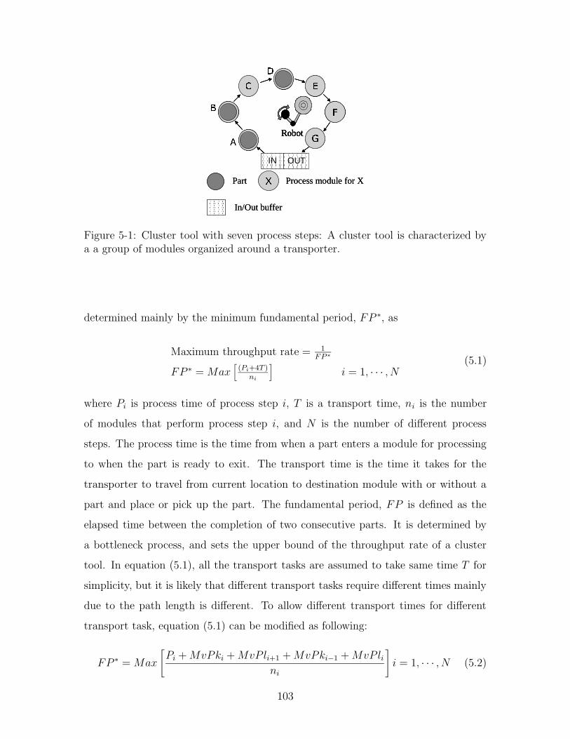
�� Robot

��

�

� �Robot


In/Out buffer

IN OUT

��

��

�� Robot

��

�

� �Robot


In/Out buffer

� � � � � � � � � � � � � �� IN OUT

Figure 5-1: Cluster tool with seven process steps: A cluster tool is characterized bya a group of modules organized around a transporter.

determined mainly by the minimum fundamental period, FP ∗, as

Maximum throughput rate = 1FP ∗

FP ∗ = Max[

(Pi+4T )ni

]

i = 1, · · · , N(5.1)

where Pi is process time of process step i, T is a transport time, ni is the number

of modules that perform process step i, and N is the number of different process

steps. The process time is the time from when a part enters a module for processing

to when the part is ready to exit. The transport time is the time it takes for the

transporter to travel from current location to destination module with or without a

part and place or pick up the part. The fundamental period, FP is defined as the

elapsed time between the completion of two consecutive parts. It is determined by

a bottleneck process, and sets the upper bound of the throughput rate of a cluster

tool. In equation (5.1), all the transport tasks are assumed to take same time T for

simplicity, but it is likely that different transport tasks require different times mainly

due to the path length is different. To allow different transport times for different

transport task, equation (5.1) can be modified as following:

FP ∗ = Max

[

Pi +MvPki +MvPli+1 +MvPki−1 +MvPlini

]

i = 1, · · · , N (5.2)

103

where MvPki is the time it takes for a transporter to move to process i module and

pick up a part, MvPlj is the time it takes for the transporter to move to process

j module and place a part. (+1) and (-1) in the subscripts indicate the next and

previous process step, respectively. For example, when i = 1, (i−1) is [In] and (i+1)

is 2. One of the assumptions made in deriving equation (5.1) and (5.2) is that when

it is empty-handed, the robot waits at its current position, and only begins moving

toward a destination module after the process therein is complete. It is sometimes

called as simple scheduling. Another assumption is that the system is in ’process-

limited mode’ of operation, meaning that one of the process modules is a bottleneck

of the system as opposed to the transporter being a bottleneck. For further details

on determining fundamental period, readers are recommended to refer to [30],[32].

5.1.2 Scheduling for Deterministic System

Scheduling in a cluster tool can be defined as assigning a sequence of transport tasks

to transporter(s). It can be a fixed sequence repeated over and over, or can be a long

sequence without a repeatable pattern. The most fundamental functional requirement

for scheduling task is to ‘transport a part from one station to the next station when

the current station finishes its processing on the part.’ In rare cases, a transporter may

be able to simply respond to all the transport requests without any trouble. If that

is the case, a schedule is simply the result of a transporter’s responding to transport

requests. One extreme example of such case is a system with only one process step

with one transporter. All it needs to do is to pick a finished part up from the process

module and place it to [Out] buffer, and pick up a new part from [In] buffer to place

it into the process module. With no complication, the simple sequence repeats itself.

However, except for a few instances, it is very likely that there is a situation where

two or more parts need to be transported nearly at the same time. Such situation

is called a conflict: a conflict between multiple transport tasks that share the same

transporter. Those conflicts can be resolved by various means, and depending on

the way they are resolved, different schedules will be obtained. Thus, scheduling

becomes an active design task rather than passive outcome of transporter’s reactions

104

to transport requests. Depending on which part is picked first by the transporter, the

subsequent pattern of the part flow and the subsequent schedule of the transporter

motion will be different. Each one of the decision points is a bifurcation point and

therefore, the number of the possible combinations for the flow paths for the parts and

for the transporter motion will increase with the number of such decisions made. Such

a system is defined as a time-dependent combinatorial complexity system – a system

in which follow-on decisions are always affected by previous decisions, increasing the

number of possible combinations.

Reacting to the conflict based on predetermined priority rules is one way to resolve

the conflicts. Planning a synchronized transport/process pattern is another way of

handling the problem [33],[32],[37]. Typically, the goal of scheduling is to achieve the

throughput time1 as close to FP ∗ as possible. In most cases, however, that is not

the only objective. Oftentimes, other objectives, such as minimizing makespan2 is

pursued, which makes the scheduling an optimization problem. Also, it is common

that scheduling is subject to process constraints, e.g. ‘a part has to leave the process

module immediately when the module finishes its process on the part.’

A cluster system is said to be deterministic if all the process times are constant,

transport times are constant and it does not have random events such as machine

breakdown. Although it is far from realistic assumption, a deterministic model char-

acterizes a system in terms of upper/lower bound of the system performance. For

deterministic system, the maximum performance – upper bound of the throughput

rate – is known to be FP ∗ which can be readily computed by equation 5.1 and 5.2.

Unless the system is handled erroneously, a deterministic system reaches a steady

state with its own fundamental period. Then, the goal of scheduling is to mini-

mize ∆ = (Actual throughput time) − FP ∗ while satisfying other objectives and

constraints.

As mentioned previously, top level functional requirement for scheduling is to

‘transport a part from one station to the next station when the current station finishes

1Throughput time is (throughput rate)−1. Sometimes, it is referred to as cycle time.

2Makespan: Time it takes for a system to process a batch, i.e. from when the first part entersthe system to when the last part of the batch leaves the system

105

its processing on the part.’ Given the process recipe and system configuration, a fixed

set of sub-level functional requirements can be explicitly defined:

Transport a part from [In] to M1 = FR0

Transport a part from M1 to M2 = FR1

Transport a part from M2 to M3 = FR2

:

Transport a part from MN to [Out] = FRN

Since the functional requirements appear at different times, ui(t) can be used to

appropriately represent these FRs. Recall the function state variable, ui(t) defined

by equation 3.6 and 3.7 in chapter 3.

ui(t) =

ui for t ≥ τi

0 for t < τi

(5.3)

u(t) = {u0(t), u1(t), . . . , uN (t)} (5.4)

Then, within one period, u(t) changes from the initial state, u(0) = {0, 0, · · · , 0}

to the final (completion) state, u(T) = {1, 1, · · · , 1}. The number of total (feasible &

infeasible) transition patterns is (N + 1)!. Particular transition pattern corresponds

to a particular schedule. Some of these patterns represent feasible patterns, and oth-

ers do not. Obviously, exhaustive search for feasible transition patterns and selecting

the best one by evaluating all of them is not an economic way to obtain the solution.

The priority-based ‘if-then’ type of reactive scheduling can be used as an alterna-

tive, but its developing process could be time-consuming because every single conflict

situation has to be addressed by rules. Indeed incomplete set of rules can develop

time-dependent combinatorial complexity in a system, and eventually fail the system.

Furthermore, it does not ensure the throughput rate until the priority rules are vali-

dated collectively. Better alternative is to deploy a deterministic scheduling scheme.

Since the deterministic system is completely predictable, we can effectively maintain

106

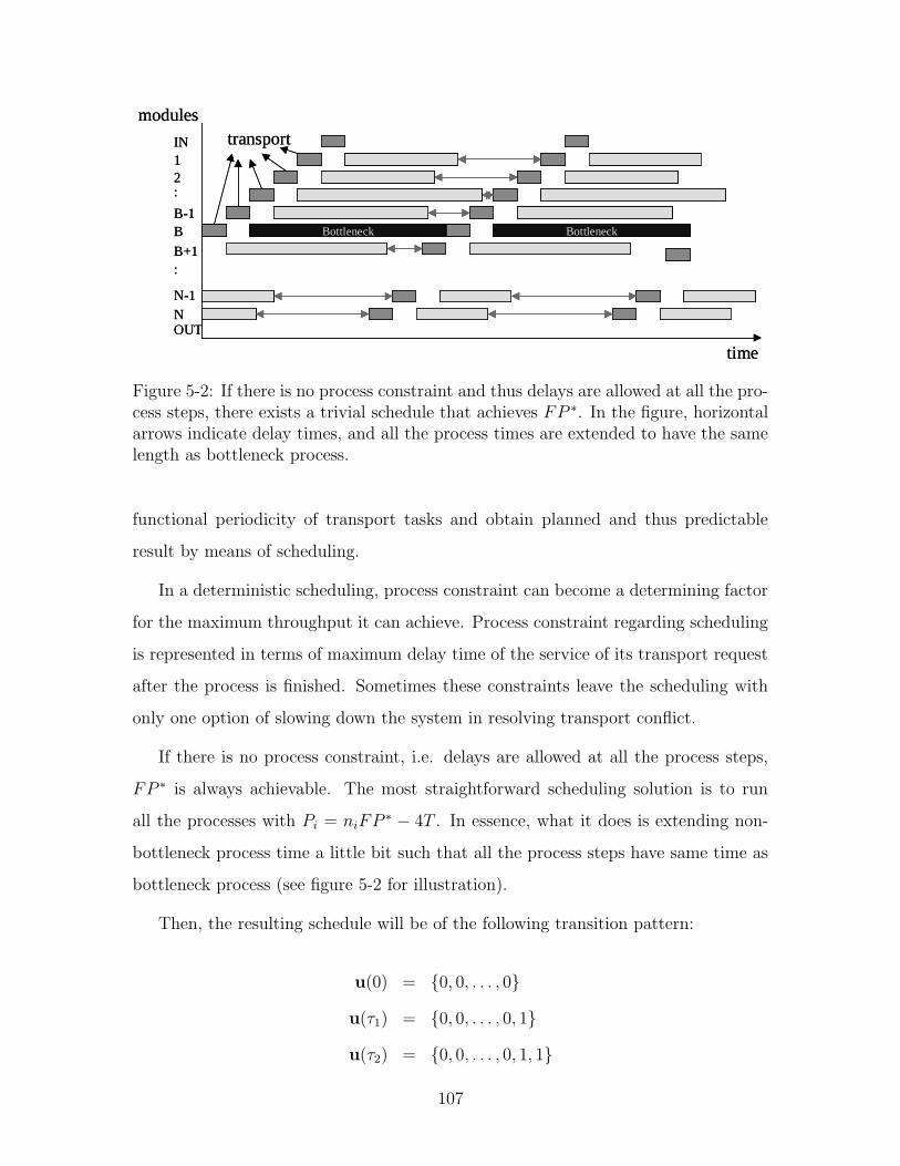
OUTNN-1

:B+1

BB-1

:21IN

time

Bottleneck Bottleneck

modulestransport

OUTNN-1

:B+1

BB-1

:21IN

time

Bottleneck BottleneckBottleneck BottleneckBottleneck Bottleneck

modulestransport

Figure 5-2: If there is no process constraint and thus delays are allowed at all the pro-cess steps, there exists a trivial schedule that achieves FP ∗. In the figure, horizontalarrows indicate delay times, and all the process times are extended to have the samelength as bottleneck process.

functional periodicity of transport tasks and obtain planned and thus predictable

result by means of scheduling.

In a deterministic scheduling, process constraint can become a determining factor

for the maximum throughput it can achieve. Process constraint regarding scheduling

is represented in terms of maximum delay time of the service of its transport request

after the process is finished. Sometimes these constraints leave the scheduling with

only one option of slowing down the system in resolving transport conflict.

If there is no process constraint, i.e. delays are allowed at all the process steps,

FP ∗ is always achievable. The most straightforward scheduling solution is to run

all the processes with Pi = niFP ∗ − 4T . In essence, what it does is extending non-

bottleneck process time a little bit such that all the process steps have same time as

bottleneck process (see figure 5-2 for illustration).

Then, the resulting schedule will be of the following transition pattern:

u(0) = {0, 0, . . . , 0}

u(τ1) = {0, 0, . . . , 0, 1}

u(τ2) = {0, 0, . . . , 0, 1, 1}

107

u(τ3) = {0, 0, . . . , 0, 1, 1, 1}

...

u(τn+1) = {1, 1, . . . , 1}

Although it may not be the best schedule in a sense that the delay times may be

excessive, it certainly is one of the scheduling solution that deliver FP ∗.

At the other extreme where all the delays are completely prohibited, FP ∗ is un-

likely to be achievable. If there exists any conflict when the system runs at throughput

rate of (FP ∗)−1, then the only degree of freedom to resolve conflict is its sending pe-

riod – time between part-feeding into the system. Since the sending period cannot

be shorter than FP ∗, using longer sending period is the only way to resolve conflicts.

In such case, r-part cyclic schedule is known to be equal or better than a single-part

cyclic schedule [38],[39][40]. In r-part cyclic schedule, r parts enter a system and r

parts leave the system within one period whereas a single-part cycle is defined by

one-part leaving and entering a system (see figure 5-3). In terms of sending period,

r-part cycle has r different sending periods that repeat as a whole set. 1-part cyclic

schedule is a special case of r-part cyclic schedule. In some cases, r-part cycle is

better than 1-part cycle, delivering higher throughput rate. Since 1-part cycle is a

special case of r-part cycle, r-part cycle can be said to be equal or better than 1-part

cyclic schedule. Consider, for example, a system with five process steps each with a

single process module [38]. Processing times Pi are as following: P1=3, P2=5, P3=3,

P4=4, P5=2. As shown in figure 5-3, while 1-part cycle delivers throughput time of

13 time units, the 2-part cycle that consists of sending periods of 7 and 13 units is

able to deliver throughput time of average of 10 units.

In r-part cyclic schedule, a set of r sending periods repeat themselves as the system

processes more than r parts. On the contrary, there can be a schedule that is perfectly

feasible for r parts but not repeatable for subsequent parts. This type of schedule is

called acyclic schedule. If we know that there will be exactly k parts to be processed,

we can come up with k-part acyclic schedule. In terms of maximum throughput rate,

this k-part cyclic schedule is equal or better than r-part cyclic schedule (r ≤ k) [40].

108

� � � � � � � � � � � � � � � � � � � � � � � � � � � � � � � � � � � � � � � � � � � � � � � � � � � � � � � � � � � � � � � � � ��

� � � � � � � � � � � � � � � � � � � � � � � � � � � � � � � � � � � � � � � � � � � � � � � � � � � � � � � � � � � � � � � � � �

� � � � � � � � � � � � � � � � � � � � � � � � � � � � � � � � � � � � � � � � � � � � � � � � � � � � � � � � � � � � � � � � � ��

� � � � � � � � � � � � � � � � � � � � � � � � � � � � � � � � � � � ��

a b c d e

SP1 = 13 a b c d e

SP1 = 13 a b c d

a b c d e

SP1 = 13 a b c d e

SP2 = 7 a b c d e

SP1 = 13 a b

(a) Best 1-part cycle at SP = 13 time unit

(b) Best 2-part cycle at SP1 = 13 time unit and SP2 = 7 time unit

Figure 5-3: (a) 1-part cycle gives a throughput rate of 113

while 2-part cycle shown in(b) yields higher throughput rate of 1

10

That is because the repeatability is, in a sense, a constraint in finding a scheduling

solution. 10-part cyclic schedule for 10 parts to process may be different from acyclic

schedule, and acyclic schedule may be better than cyclic schedule. However, it should

be noted that obtaining r-part acyclic schedule becomes computationally hard as r

gets large [40],[41].

Less extreme is the scheduling with some process constraints. Some of the process

steps require zero delay time for the part transport, but others are not so critical that

they can be used as temporary buffers. In such case, whether FP ∗ is achievable or not

depends on the conflict pattern with respect to the process constraints. For example,

suppose the process step j requires zero delay and conflict occurs between transport

[j → (j + 1)] and transport [(j − 1) → j]. If it were not for the constraint, delaying

the transport [j → (j + 1)] will resolve the conflict without necessarily slowing down

the system. However, due to the constraint, the only way to resolve the conflict is

to increase the sending period until the conflict is gone. In this example, the process

constraint on j is the limiting factor for the system’s throughput rate. If none of

process constraints is limiting factor, then the system will be able to achieve FP ∗ by

properly assigning delay times to non-critical process steps [32],[37].

If process constraint is limiting factor, it is easy to see that multi-part cycle may

deliver better throughput by the same reasoning in the case with fully-constrained

109

scheduling. r-part cycle implies a set of r sending period and possibly a set of r dif-

ferent delay times at non-critical process steps. However, in some cases, non-uniform

delay times for different parts could result in inconsistent quality since different parts

will experience different delay times.

To summarize, if delays are allowed at all the process stations, maximum through-

put rate can always be achieved at (FP ∗)−1. If a system is fully constrained, FP ∗

is unlikely to be achievable since even a single conflict cannot be resolved without

slowing down the system. For such system, multi-part cycle solution is equal or bet-

ter in terms of throughput rate than one-part cycle solution. However, finding the

global optimum solution, i.e. finding r∗ for r-part cyclic schedule that yields the best

throughput rate, is known to be computationally hard problem. If a system is par-

tially constrained at some of its process stations, the existence of schedule solution to

achieve FR∗ depends on constraints: process constraints may not be a limiting factor

and thus do not rule out a schedule for FP ∗. Or they render the scheduling problem

to be similar to fully-constrained problem and thereby force to slow down the sys-

tem. r-part cycle may give a better result. But then consistency in product quality

may be a problem because parts in different groups will experience different delay

times. In any case, preserving periodicity can take the benefit of the predictability in

a deterministic system, and result in predictable system performance.

Non-deterministic case is different form deterministic case, and the solution ob-

tained from the deterministic case would not work. Next section discusses the schedul-

ing problem for non-deterministic problem, and an interesting example is presented

to illustrate the consequence of the loss of periodicity. Also, a means of maintaining

functional periodicity, re-initialization, is discussed.

110

5.2 Maintaining a Periodicity in a Manufacturing

System

When two different subsystems with two different throughput rates are joined to-

gether, they must be integrated to maximize the productivity of the entire system.

Consider a simple system consisting of subsystem X and subsystem Y, which are

physically connected to each other to make a product. Both subsystems may consist

of many physical modules to process a part by subjecting it to a variety of different

processes that require different process times. The process time in each module is

different and specific to the part to be made. In addition, although the nominal pro-

cessing times are set for each subsystem, the throughput rate of each subsystem may

vary from the nominal value if there are variations in the processing times.

Obviously the modules in subsystems will complete their processes at different

times because parts arrive in each module at different times and also because their

process times are different. Furthermore, there will be inevitable random variations

in the process times of individual modules in the subsystems. Some of these parts

will be finished nearly at the same time, waiting to be picked up by a transporter –

hereinafter referred to as a robot – for the next operation. The role of scheduling is

to resolve such conflicts. Conflicts should be resolved such that the system does not

have a time-dependent combinatorial complexity since a system with combinatorial

complexity may not be able to achieve the maximum theoretical throughput rate.

For such a system to have the maximum productivity, it must be transformed into a

system with time-dependent periodic complexity. The reduction of the system com-

plexity through the transformation will maximize the productivity. In deterministic

case, the conflict pattern is predictable a priori, and thus appropriate schedule can be

constructed off-line to avoid combinatorial complexity. To create a system with time-

dependent periodic complexity in the presence of random variations, we introduce the

concept of “re-initialization.” Upon re-initialization, the initial states may vary due

to unexpected variations in process times as well as other reasons. Re-initialization

requires the following: (1) existence of a functional period in which all the functions

111

� � � � � � � � � � � � � � � � � � �� Md

� � � � � � � � � � � � � � � � � � ��

� � � � � � � � � � � � � � � � � � ��

Mc

� � � � � � � � � � � � � � � � � ��

In Out� � � � � � � � � � � � � � � � � � � � � � � � � � � � � � � � � � � � � � � � � � � � � � � ��

Subsystem Y

Subsystem X

Ma

Mb

� � � � � � � � � � � � � � � � � � �� Md

� � � � � � � � � � � � � � � � � � ��

� � � � � � � � � � � � � � � � � � ��

Mc

� � � � � � � � � � � � � � � � � ��

In Out

Subsystem Y

Subsystem X

Ma

Mb

Figure 5-4: Subsystem X and Y are joined together to subject wafers to a series ofprocesses.

are repeated, (2) at the beginning of each period, establishment of new initial con-

ditions, and (3) determination of the best schedule for the entire process from the

newly established initial conditions. The period begins when a key function – either

triggered internally or externally – re-initializes the system. We will demonstrate the

process using an example.

5.2.1 Example: Wafer Processing System

Consider a hypothetical wafer processing system3. The system is to be created by

integrating two subsystems X and Y. Figure 5-4 depicts a physical configuration of

the system under consideration. The configuration is characterized by a transporter

surrounded by multiple process machines – cluster tool. Subsystem X performs four

different functions in a given sequence, a, b, c, and d, to produce patterns on a wafer

continuously. Subsystem Y takes the semi-finished part from subsystem X and sub-

jects them to subsequent processes. Processes a through d are performed in subsystem

X by machine Ma through Md, respectively. Each machine Mi processes only one part

at a time. A robot located in subsystem X transports parts between machines in sub-

system X, and passes it on to subsystem Y. Process sequence along with specified

3This example is based on [42]

112

process times is often called a process recipe. The number of machines for each of

process steps is determined based on the process times and required throughput rate.

If a particular process step takes too long to meet required throughput rate, then

additional machine is added to the process step. For example, if the throughput time

requirement is 60 seconds and process a takes 80 seconds, then two machines, Ma,1

and Ma,2 are required to meet the target throughput time. This set of machines to

perform the same process step, {Ma,1,Ma,2}, is referred to as station a, Sa. Given

the system configuration along with process sequence, functional requirements for the

transporter is explicitly stated as following:

Transport a wafer from [In] to Sa = FR0

Transport a wafer from Sa to Sb = FR1

Transport a wafer from Sb to Sc = FR2

Transport a wafer from Sc to Sd = FR3

Transport a wafer from Sd to [Out] = FR4

The process time Pi for each of the process steps is the time between receipt of a

part and completion of the processing at machine Mi (when the part is ready to leave

Mi). The cycle time CTY of subsystem Y is defined as the time between receipt of a

part at subsystem Y and removal of the part from subsystem Y (when subsystem Y

is ready to take a new part).

In this example, we assume that the cycle time of subsystem Y varies significantly

compared to the variation of process times of subsystem X. Also, process c is assumed

to be critical such that a part in machine Mc must be removed as soon as process c

is completed. It is further assumed that considerations of economic efficiency render

the maximum utilization rate of subsystem Y highly desirable.

Equation (5.2) can be modified to better model the throughput of the integrated

system. In a particular setup of this example, FP of the whole system is determined

by the slower of the two subsystems. If subsystem X determines the pace of the

113

integrated system, fundamental period of the system is given by

FP = FPX

= Max

[

Pi +MvPki +MvPli+1 +MvPki−1 +MvPlini

]

(5.5)

i = a, b, c, d

If subsystem Y is slower than subsystem X, the fundamental period of the integrated

system is given by

FP = FPY = CTY +MvPkY −1 +MvPlY (5.6)

where MvPkY −1 is the time for the robot to move to the last process stage Sd in

subsystem X and pick up a part, and MvPlY is the time for a robot to move the part

to subsystem Y (Out). The fundamental period of the overall system, FP , is given

by the larger of FPX and FPY . That is,

FP = Max [FPX , FPY ] (5.7)

The following three cases illustrate the re-initialization of systems to achieve time-

dependent periodic complexity for different subsystem throughput relationships.

Case 1 Subsystem X is slower than subsystem Y: FPX > max[FPY ]

Case 2 Subsystem X is faster than subsystem Y: FPX < min[FPY ]

Case 3 Both subsystems are at approximately same speed: FPX ≈ FPY , i.e.

min{FPY } < FPX < max{FPY }

In each case, the maximum productivity (i.e. throughput rate) is attained when the

operations of the subsystems are subject to a repeated re-initialization implemented

after the completion of subsystem cycle. Re-initialization introduces periodicity and

thus changes the scheduling problem from that of a time-dependent combinatorial

complexity to a time-dependent periodic complexity problem. Each of the cases will

be considered separately.

114

Station Pi or CTY Number of machines MvPki MvPliIn - 1 5 -

a 30 1 5 5X b 40 1 5 5

c 60 1 5 5d 80 2 5 5

Y 60±5 1 - 5

Table 5.1: Parameters for Case 1

Case1: FPX >max[FPY ]

Case 1 addresses a system in which FPX is larger than FPY . As a consequence of

subsystem Y’s being faster than subsystem X, subsystem Y has to wait until a next

part finishes its processes in subsystem X. In other words, subsystem Y is operated

in a ‘starved’ mode. Therefore, it does not matter when subsystem Y finishes its

process and requests a new part as long as this relationship between FPX and FPY

holds. In short, the variation of CTY does not affect subsystem X’s operation. The

maximum productivity is achieved simply when the throughput of the integrated

system reaches that of subsystem X. Table 5.1 shows the process times for processes

a, b, c, d, the cycle time for subsystem Y, the number of machines for each process,

and the associated transport times.

According to equations (5.5), FPX is 80 seconds. As stated earlier, CTY is as-

sumed to vary within ±5 seconds, i.e. CTY = 55 ∼ 65 seconds. Thus, by equation

5.6, FPY is 65 ∼ 75 seconds. Given FPX and FPY , the fundamental period FP of

the integrated system is 80 seconds.

As mentioned above, subsystem Y operates in a starved mode since FPX is larger

than the maximum FPY . Therefore, variation in subsystem Y’s cycle time, 55∼65

seconds, will not affect the scheduling. Even if subsystem Y requests a wafer as it

is ready to process the next one, no wafer is available from subsystem X, and thus

subsystem Y has to wait for a while. The variation in CTY needs not be considered

in subsystem X’s transport scheduling. Since there is no variation issue in scheduling,

the steady state scheduling can be directly used.

To solve this problem, it is very useful to visualize the situation using a timing

115

Y START Y FINISHCTY = 60 sec

1 2

3 4 machine d2 1 2

b 5 6 machine c 3 4 machine d1 1 2

9 10 machine a 7 8 machine b 5 6 machine c 3 4

SENDING PERIOD = 80sec 9 10 machine a 7 8 machine b 5 6

SENDING PERIOD = 80sec 9 10 a

Y START Y FINISHCTY = 60 sec

1 2

3 4 machine d2 1 2

b 5 6 machine c 3 4 machine d1 1 2


SENDING PERIOD = 80sec 9 10 machine a 7 8 machine b 5 6


Figure 5-5: Part-flow timing diagram. Each row represents the individual panelsbeing processed by different machines. Transport task (3 4)-(9 10) and (1 2)-(5 6)are in conflicts.

diagram. Figure 5-5 is a part-flow timing diagram. The horizontal axis represents

time and the vertical axis (row) represents different parts processed by the system. In

particular, the first row represents the flow of a first part processed by the system, the

second row represents the flow of the second part processed by the system, etc. Since

FP is constant at 80 seconds, the incoming parts are assumed to be 80 seconds apart

from each other in steady state. In other words, the sending period is set to equal FP

of the system. Figure 5-5 shows that there are two transport conflicts between trans-

port task [1 2]-[5 6] and [3 4]-[9 10], and the conflicts occur repeatedly. It is clear that,

depending on which part is picked up first by the robot at the moment of the conflict,

the subsequent pick-up schedule will be affected by the decision. Thus, the number

of possible routes for the robot increases as additional decisions are made at the time

of the conflicts. The system is therefore subject to time-dependent combinatorial

complexity. To reduce the number of possible combinations and thereby facilitate

the robot scheduling, this time-dependent combinatorial complexity problem must

be converted into a time-dependent periodic complexity problem. If a sending period

and delay times at some of the process steps are appropriately selected, the complexity

of the subsystem X can be converted into a time-dependent periodic complexity.

From Figure 5-5, one can easily see, by inspection, that 10 seconds of post-process

delay time in machine Mb and another 10 seconds post-process waiting time in Md

will simply resolve these conflicts without the need for real-time decision-making. In

other words, those waiting times prevent conflicts from occurring at the first place.

116

� � � � � � � � � � � � � � � � � � � � � ��

� � � � � � � � � � � � � � � � � � � � � � ��

� � � � � � � � � � ��

Y START Y FINISHCT Y = 60 sec

machine d1 1 2 Y START

c 3 4 machine d2 1 2

b 5 6 machine c 3 4 machine d1


SENDING PERIOD = 80sec 9 10 machine a 7 8 machine b


Figure 5-6: 10 seconds post-process delay times at process b and d resolve the conflicts.

Figure 5-6 shows such scheduling solution with the waiting time indicated by hatched

area. Note that the time subsystem Y starts processing is determined by subsystem

X, which is not affected by the variation in CTY . This solution gives the following

periodic u(t):

u(0) = {0, 0, 0, 0, 0}

u(τ0) = {1, 0, 0, 0, 0}

u(τ3) = {1, 0, 0, 1, 0}

u(τ2) = {1, 0, 1, 1, 0}

u(τ4) = {1, 0, 1, 1, 1}

u(τ1) = {1, 1, 1, 1, 1}

u(FP ) = {0, 0, 0, 0, 0}

Case 1 is equivalent to a scheduling problem with no variation since subsystem

X, that has no process time variation, determines the pace of the whole system.

Therefore, steady-state scheduling method such as [32] can be used directly to provide

scheduling solution as in Figure 5-6.

Case2: FPX < FPY

Table 5.2 shows the process times for processes a, b, c, d, the cycle times for subsystem

Y, the number of machines for each process, and the associated transport times.

Based on the equations (5.5)-(5.7), the fundamental period of the integrated system

117

Station Pi or CTY Number of machines MvPki MvPli

In - 1 5 -a 30 1 5 5

X b 40 1 5 5c 50 1 5 5d 80 2 5 5

Y 80±5 1 - 5


Y STARTCT Y = 80 sec Y FINISH

1 2 Y STARTCT Y = 80 sec Y FINISH

3 4 machine d2 1 2

machine b 5 6 machine c 3 4 machine d1 1 2


New panel SP=90sec 9 10 machine a 7 8 machine b

New panel SP=90sec

Y STARTCT Y = 80 sec Y FINISH

1 2 Y STARTCT Y = 80 sec Y FINISH

3 4 machine d2 1 2

machine b 5 6 machine c 3 4 machine d1 1 2


New panel SP=90sec 9 10 machine a 7 8 machine b

New panel SP=90sec

Figure 5-7: Steady state scheduling solution with CTY at constant 90 seconds

is determined by subsystem Y to be 85∼95 seconds. If CTY were constant at 80

seconds, which would yield 90 seconds of FPY , assigning appropriate delay times

with the system’s sending period set to 90 seconds would simply solve the scheduling

problem as in case 1. The pattern shown in Figure 5-7 would be one of legitimate

scheduling solutions that repeat itself. However, as opposed to Figure 5-7, the pattern

of timing diagram under the variation will not be the same for each period. Subsystem

Y takes a part from subsystem X once every 85∼95 seconds non-deterministically, and

thus the temporal location of the transport task from subsystem X to Y, [1 2], is not

fixed with respect to other transport tasks. Therefore, the constant waiting time

solution as in Figure 5-7 is not valid, and the schedule for robot motion must be

recomputed each time subsystem Y picks up a semi-finished part from subsystem X.

Recall that there are two constraints on subsystem X. First, the part just processed

at machine Mc must be immediately picked up for transport. Second, a part and the

robot must be available for subsystem Y when it is ready to take the part. Depending

on the variation in the cycle time CTY and the inherent conflict patterns, the task of

scheduling can be significantly unfavorable. In particular, the difficulty in scheduling

118

results from the randomness in the transport conflict pattern due to CTY variation.

The variation in CTY along with decisions made at ‘current’ conflict can lead to

combinatorial complexity. As previously described, time-dependent combinatorial

complexity problem must be converted into a periodic complexity problem. The

conversion requires that a functional period be imposed on the system. In such a

period, the same set of tasks are performed cyclically and, therefore, a limited number

of scheduling possibilities exist. The period is initiated by an internal or external key

event, or re-initializing event, that needs to be appropriately defined. In this example,

a part-request from subsystem Y, FR4 is chosen to be the re-initializing event for three

reasons. First, subsystem Y limits the pace of the integrated system. Also, the pace of

the integrated system has to be adjusted to accommodate the variations in the cycle

time of subsystem Y. Third reason is that a basic constraint on the system requires

that delivery of a part to subsystem Y be completed immediately upon the request.

Because a part-request issued by subsystem Y is treated as the re-initializing event,

the length of each period depends on CTY . Even though the length of each period is

generally different, the same set of functions, i.e. transport tasks, are completed by

the robot in the subsystem X within each period.

The central idea is to force the system to have a periodicity whose initiation

is defined by the re-initializing event that is FR4. At the time of re-initialization,

the current state of subsystem X – which machines are available and the remaining

process times of occupied machines – is determined. Appropriate delay times are

then calculated for each of the occupied machines, which determines a schedule for

the current period. First, to ensure that the robot is always available during the time

slot of the next re-initializing event, a no-transport-time interval is defined:

No transport time =

{t|t ∈ [(MvPkY −1 +MvPlY ) +min[CTY ], (MvPkY −1 +MvPlY ) · 2 +max[CTY ]]}

where t=0 at the moment of the current re-initializing event. Transport of parts must

be scheduled such that none of the transport tasks is assigned during this time interval

119

� � � � ��

� � � � � � � � � � � � � � � � � � � � � � � � � � � � � � � � � � � � � � � � � � � � � � � � � � � � � � � � � � � � � � � � � � � � � � � � � � � � � � � � � � � � � � � � � � � � � � � � � � � � � � � � � � � � � � � � � � � � � � � � � � � � ��

� � � � � � � � � � � � � � � � � � � � � � � � ��

� � � � � � � � � � � � � � � � � � � � � � � � � � � � � � � � � ��

Y FINISHY START

CT Y = 80 sec Y FINISH1 2 Y START

Y FINISHMachine d2 1 2 CT Y = 80 sec Y START

Max[CT Y] = 85 secMachine c 3 4 Machine d1 1 2

Min[CT Y] = 75 secMachine b 5 6 Machine c 3 4 Machine d2

Machine a 7 8 Machine b 5 6 Machine c Transport (next period)

SP=90sec 9 10 Machine a 7 8 Machine b

SP=90sec 9 10 Machine a

Instant of Reinitialization

Figure 5-8: Variation in subsystem Y’s cycle time

to ensure immediate delivery of parts to subsystem Y. Second, assign all transport

tasks which are determined at the instant of re-initialization (i.e., pre-fixed transport

tasks). Pre-fixed tasks include transport [1 2] by the definition of the re-initializing

event, and transport [3 4] due to the process constraint at machine Mc. Remaining

transport tasks are then allocated accordingly. Figure 5-8 depicts a part-flow timing

diagram for the steady state operation, showing a potential variation in cycle time

CTY at the right end. The vertical lines indicate the time when subsystem Y requests

a part from subsystem X and therefore represent the moment of re-initialization. As

shown in the last period, due to the variation in CTY , subsystem Y requests a semi-

finished part from subsystem X at some time at least 85 seconds but no more than 95

seconds after the re-initialization (75∼85 second cycle time plus 10 second transport

time for [1 2]). Therefore, the transport task is scheduled so that the robot is available

for the period from 85 seconds to 105 seconds after the re-initialization.

After a part-request is issued by subsystem Y (vertical line), a renewal signal is

generated to re-initialize the database of processes. First, the state of each machineMi

is identified as busy or idle, and empty or occupied. For example, at the onset of the

second re-initialization (second vertical line), the following information is identified:

Empty {}

Busy { Ma, Mb, Mc, Md2 }

Occupied { Md1 }

Once busy machines are identified, their remaining process times are monitored.

120

t' = initialized t 0 5 10 15 20 25 30 35 40 45 50 55 60 65 70 75CTY 0 5 10 15 20 25 30 35 40 45 50 55 60 65

stateMachine a 15 aMachine b 15 bMachine c 15 cMachine d1 ocpMachine d2 15 d2

t' = initialized t 0 5 10 15 20 25 30 35 40 45 50 55 60 65 70 75CTY 0 5 10 15 20 25 30 35 40 45 50 55 60 65


Figure 5-9: Information at the instant of re-initialization

t' = initialized t 0 5 10 15 20 25 30 35 40 45 50 55 60 65 70 75 80 85 90 95 ##CTY 0 5 10 15 20 25 30 35 40 45 50 55 60 65 70 75 80

stateMachine a 15 a 7 8 9 10 aMachine b 15 b 5 6 bMachine c 15 c 3 4 IDLE c 3 4Machine d1 ocp 1 2 d1Machine d2 15 d2

robot 1 2 3 4 5 6 7 8 9 10 X X X X

t' = initialized t 0 5 10 15 20 25 30 35 40 45 50 55 60 65 70 75 80 85 90 95 ##CTY 0 5 10 15 20 25 30 35 40 45 50 55 60 65 70 75 80

stateMachine a 15 a 7 8 9 10 aMachine b 15 b 5 6 bMachine c 15 c 3 4 IDLE c 3 4Machine d1 ocp 1 2 d1Machine d2 15 d2

robot 1 2 3 4 5 6 7 8 9 10 X X X X

Figure 5-10: [1 2], [3 4] are pre-fixed. No-transport-time is indicated by X’s.

Figure 5-9 depicts the remaining process times for the busy machines. Based on this

information, the transport schedule is constructed. In this example, no-transport-time

is {t′|85 < t′ < 105}. Transport task [1 2] and [3 4] are pre-fixed tasks. Transport

task [1 2] occurs 0 to 10 seconds after the moment of re-initialization. Another

task, [3 4] must occur from 15 to 25 seconds after re-initialization because the part

in machine Mc must be removed as soon as process c is complete. The allowable

transport timeslots are computed and the remaining transport tasks are assigned in

the timeslots. One possible schedule is shown in Figure 5-10 in which the X’s signify

the no-transport-time interval. Transport task [5 6] is delayed for a while due to

the no-transport-time condition for the following task [3 4] in the next period. This

delay indeed ensures every transport task appears exactly once in a period as well as

maximizes utilization of subsystem Y. Transport tasks [7 8] and [9 10] simply follow

task [5 6] at the earliest possible time according to fundamental conditions for part

transport – the current machine is finished, the next machine is empty, and the robot

is available.

By applying the above-mentioned approach repeatedly, schedule for the next pe-

121

Y FINISH Y START1 2

CT Y = 80 sec Y FINISH Y STARTd2 1 2

CT Y = 75 sec Y FINISHc 3 4 Machine d1 1 2 Y START

85 secb 5 6 Machine c 3 4 Machine d2 1 2

a 7 8 Machine b 5 6 Machine c 3 4 Machine d1

9 10 Machine a 7 8 Machine b 5 6 Machine c 3 4

New panel SP=90sec 9 10 Machine a 7 8 Machine b

New panel SP=85sec 9 10 Machine a

New panel SP=95sec

Y FINISH Y START1 2

CT Y = 80 sec Y FINISH Y STARTd2 1 2

CT Y = 75 sec Y FINISHc 3 4 Machine d1 1 2 Y START

85 secb 5 6 Machine c 3 4 Machine d2 1 2

a 7 8 Machine b 5 6 Machine c 3 4 Machine d1

9 10 Machine a 7 8 Machine b 5 6 Machine c 3 4

New panel SP=90sec 9 10 Machine a 7 8 Machine b

New panel SP=85sec 9 10 Machine a

New panel SP=95sec

Figure 5-11: Resulting schedule for case 2

riod can be determined relatively easily regardless of when subsystem Y picks up the

part exiting subsystem X. Figure 5-11 depicts multiple intervals with different cycle

times CTY for subsystem Y, and it is clear that the variation is well accommodated.

Indeed, every interval is independent from the previous intervals except for the im-

mediately preceding interval. In other words, the initial state of u(0) is attained

repeatedly so that the effect from the variation of the CTY does not propagate to the

later periods.

Case3: FPX ≈ FPY

Case 3 is a mixture of case 1 and case 2 because FPY is sometimes less than the

FPX and at other times is larger than FPX . It is tempting to think that the effect of

the period where subsystem Y is slower is canceled out by that of faster periods over

the long run, and thus it is possible to operate subsystem X at subsystem Y’s pace.

Unfortunately, the faster period, when CTY has the value of min[CTY ], cannot be

used to directly offset the slower period, when CTY is max[CTY ], because the duration

of the actual cycle time CTY for the next period is not known a priori. Since it is not

known when subsystem Y will request its next part, subsystem X has to be ready to

deliver a part at the earliest possible request time by subsystem Y if it is to satisfy

the constraint of maximum utilization of subsystem Y. Therefore, it is equivalent to

operating subsystem X at the faster pace than its maximum capability, which cannot

be achieved.

122

Station Pi or CTY Number of machines MvPki MvPli

In - 1 5 -a 30 1 5 5

X b 40 1 5 5c 50 1 5 5d 80 2 5 5

Y 60±5 1 - 5


Y FINISH

Y START Y FINISHCT Y = 60 sec Transport

1 2 Y START (next period)Max[ CT Y] = 6 5 sec

Machine d1 1 2Min[CT Y ] = 55 sec

Machine c 3 4 Machine d2

Machine b 5 6 Machine c 3 4 Machine d1

Machine a 7 8 Machine b 5 6 Machine c


SP=70sec 9 10 Machine aNew panel

New panel

Y FINISH

Y START Y FINISHCT Y = 60 sec Transport

1 2 Y START (next period)Max[ CT Y] = 6 5 sec

Machine d1 1 2Min[CT Y ] = 55 sec

Machine c 3 4 Machine d2

Machine b 5 6 Machine c 3 4 Machine d1

Machine a 7 8 Machine b 5 6 Machine c


SP=70sec 9 10 Machine aNew panel

New panel

Figure 5-12: Steady state operation with sending period of 70 seconds

The process times, number of machines and associated transport times are shown

in Table 5.3. According to equation (5.5) and (5.6), FPX is 70 seconds, and FPY is

65∼75 seconds. That is, the pace of the integrated system is sometimes determined

by subsystem X, and at other times by subsystem Y. Figure 5-12 depicts one mode

of steady state operation of subsystem X with a sending period equal to nominal FP

of 70 seconds. Limited to the illustrated instance, subsystem X appears capable of

providing a part to subsystem Y even if subsystem Y has a cycle time CTY of 55

seconds. In particular, the fundamental conditions for part-transport are satisfied

because a part is ready at machine Md2, the robot is available, and subsystem Y is

ready to accept a part. Would it be acceptable as it appears? Would subsequent

intervals with CTY of 65 seconds compensate for this short period?

Referring to Figure 5-13 - 5-19, however, it can be shown that subsystem X cannot

sustain a high system throughput over many intervals. In Figure 5-13 - 5-19, we

begin with depicting a situation where CTY is first assumed to be 55 seconds which is

123

Y FINISH Y STARTPanel # Y FINISH

0 d1 1 2 Min[CT Y] = 55 sec Y START

1 c 3 4 Machine d2 1 2

2 b 5 6 Machine c 3 4 Machine d1

3 a 7 8 Machine b 5 6 Machine c

4 9 10 Machine a 7 8 Machine b

5 New panel 9 10 Machine aSP = 70 sec X X X X

New panel No Transport

1

2

0

















1

2

0

Figure 5-13:

Y FINISHMax[CTY] = 65 sec Y START

Panel # Y FINISH2 Machine d1 1 2 Max[CTY] = 65 sec Y START

3 3 4 Machine d2 1 2

4 5 6 Machine c 3 4 Machine d1

5 7 8 Machine b 5 6 Machine c

6 9 10 9 10 Machine a 7 8 Machine bX X X X X X X X

7 No Transport 9 10 9 10

SP = 95 sec New panel SP = 75 sec

3

















3

Figure 5-14:





7 Machine a 7 8 Machine b 5 6 Machine c

8 9 10 9 10 Machine a 7 8 7X X X X X X X X

No TransportSP = 90 sec New panel





7 Machine a 7 8 Machine b 5 6 Machine c

8 9 10 9 10 Machine a 7 8 7X X X X X X X X

No TransportSP = 90 sec New panel

Figure 5-15:


Panel # Y FINISH6 d1 1 2 Max[CTY] = 65 sec


8 8 Machine b 5 6 5 6 Machine c

9 9 10 Machine a 7 8 Machine bSP = 80 sec X X X X

10 No Transport 9 10 Machine a

New panel SP = 90 sec New panel X X X XNo Transport


Panel # Y FINISH6 d1 1 2 Max[CTY] = 65 sec


8 8 Machine b 5 6 5 6 Machine c

9 9 10 Machine a 7 8 Machine bSP = 80 sec X X X X

10 No Transport 9 10 Machine a

New panel SP = 90 sec New panel X X X XNo Transport

Figure 5-16:

124


Panel #8 3 4 Machine d1 1 2


10 7 8 Machine b 5 6 Machine c 3

11 9 10 Machine a 7 8 Machine bSP = 70 sec

12 9 10 Machine aNew panel SP = 80 sec

New panel

4Y FINISH

Max[CTY] = 65 sec Y STARTPanel #



10 7 8 Machine b 5 6 Machine c 3

11 9 10 Machine a 7 8 Machine bSP = 70 sec

12 9 10 Machine aNew panel SP = 80 sec

New panel

4

Figure 5-17:

Y FINISHY START


10 4 Machine d1 1 2 Max[CTY] = 65 sec


12 7 8 7 8 Machine b 5 6 5 6 c

13 X X X 9 10 Machine a 7 8 b

14 SP = 75 sec X X X X 9New panel

SP = 100 secNew panel

5

6

6

Y FINISHY START




12 7 8 7 8 Machine b 5 6 5 6 c




Y FINISHY START




12 7 8 7 8 Machine b 5 6 5 6 c




5

6

6

Figure 5-18:

Y FINISHMax[CT Y] = 65 sec Y START

Panel # Y FINISH11 1 2 Max[CTY] = 65 sec Y START

12 Machine c 3 4 Machine d1 1 2

13 Machine b 5 6 Machine c 3 4 Machine d2

14 10 Machine a 7 8 Machine b 5 6 Machine c

15 X X X X 9 10 Machine a 7 8SP = 70 sec

New panel

7







New panel







New panel

7

Figure 5-19:

125

min[CTY ], and kept to 65 seconds, max[CTY ] afterwards. In other words, subsystem

Y is once faster than subsystem X, and it becomes slower afterward. In constructing

the timing diagram, we used simple fundamental conditions of part-transport along

with no-transport-time that was defined in case 2. Figure 5-13 - 5-19 is a series of

part-flow timing diagrams arranged in chronological order. Figure 5-14 immediately

follows Figure 5-13 in time; Figure 5-15 immediately follows Figure 5-14, and so

on. Each row in the figures is numbered according to a specific part number and the

horizontal axis represents increasing time. A throughput time is defined as the period

of time between a “Y finish” and the immediately following “Y finish”, for example

time from 0© to 1© in Figure 5-13.

In Figure 5-13, subsystem Y requests a part after it finishes its process with 55

second CTY (see 1©). Subsystem X is able to deliver a part for this early request

because machine Md2 has completed its process and waits for part number 1 to be

picked up (see 2©). Thus, when subsystem Y completes its cycle, part number 1 is

immediately provided. As a result, the throughput time for this particular period

(time from 0© to 1©) is 65 seconds. In Figure 5-14, CTY is shown to be 65 seconds.

Note that there are only four transport tasks, i.e. [1 2], [3 4], [5 6], and [7 8] in the

first interval of Figure 5-14. It is required that a no-transport-time interval of 20

seconds (indicated by two vertical lines and the X’s) be available to handle variations

in the cycle time CTY of subsystem Y. Consequently, transport task [9 10] cannot be

performed during the first interval of Figure 5-14 and is instead delayed to the next

period (see 3©).

The effect of the incomplete interval is first manifested in the elongation of sub-

sequent sending periods as well as the immediate increase of it as shown in Figure

5-14. In order to feed parts in time to subsystem Y at its 65 seconds of cycle time,

the system must have 75 seconds or shorter sending period. But, as seen from the

following figures, some of the subsequent sending periods are longer than the 75 sec-

ond. Unless there is a sufficient number of short sending periods to compensate for

those long sending periods, the integrated system will not be able to produce parts

per FP of 75 seconds due to the shortage of parts introduced into the system. For

126

the intervals up to and including Figure 5-16, subsystem X manages to follow the rate

of request from subsystem Y. In Figure 5-17, however, there is no part in subsystem

X ready to satisfy a part-request from subsystem Y (see 4©). As a result, subsystem

Y has to wait for its next part to be available. In the first interval shown in Figure

5-18, subsystem X regains its ability to immediately provide a part to subsystem Y

(see 5©). But, the no-transport-time condition in the next interval produces a long

sending period of 100 seconds (see 6©), which returns the system back to the shortage

state. Figure 5-19 shows another instance of delay in part delivery from subsystem

X to subsystem Y (see 7©). The pattern depicted in Figure 5-19 is the same as that

of Figure 5-17, thus it is obvious that the system achieves a steady state and that

the further extension of the part-flow timing diagram from Figure 5-19 is simply a

repetition of Figure 5-17 - Figure 5-19.

In constructing the diagram, it has been assumed that cycle time of subsystem Y,

CTY is 65 seconds except for the first interval. Subsystem X is faster than subsystem

Y if CTY is 65 seconds: FPY = 75 seconds > FPX = 70 seconds. Thus it might

be expected that subsystem X would evolve to a steady state operation in which the

fundamental period of the total system is 75 seconds, and that subsystem X would

always be able to feed a part to subsystem Y in time. Obviously, that will be the

case if the cycle time CTY is 65 seconds without exception. Temporal location of the

no-transport-time is fixed relative to the other robot moves, thus the same part-flow

pattern is established as the system reaches steady state. Such a case is trivial since it

is merely a transition from one steady state (FP = 70sec) to another (FP = 75sec).

Figure 5-13 - 5-19 demonstrates, however, that a single occurrence of a 55 second

CTY combined with an attempt to run subsystem X above its maximum speed –

applying no-transport-time interval – results in a degradation of system performance.

The system cannot even maintain a fundamental period of 75 seconds which it should

be able to achieve. Every fourth interval, subsystem Y must wait for an additional

25 seconds (see 4© and 7©). Thus its average throughput time in steady state is 81.25

seconds (i.e., (75+75+75+100)/4 seconds).

In this example, the longer interval of subsystem Y does not compensate for the

127

functional incompleteness in the period with shorter CTY . Even in the period with

longer CTY , in order to cover the full range of unknown variation in cycle time CTY ,

subsystem X should complete its cycle (processes and transports) within the minimum

cycle time CTY so that there is enough time to accommodate the no-transport-time

interval. If subsystem X cannot complete a cycle within one interval of CTY , it in-

evitably violates one of the requirements for re-initialization: existence of a functional

period in which all the functions are repeated. The scheduling problem becomes a

time-dependent combinatorial complexity problem lacking proper periodicity. As a

result, chances for non-optimal scheduling decisions increase and the overall system

performance can degrade. The root cause of inability to achieve the desired productiv-

ity is the attempt to run subsystem X beyond its maximum rate with a presumption

that slower periods and faster periods would nullify the effect of each other. The

attempt to overrun subsystem X caused an incomplete cycle. Consequently, it yields

a low throughput rate, which is the opposite of what was intended. This implies that

subsystem X can absorb subsystem Y’s cycle time variation only when subsystem X

is sufficiently faster than subsystem Y. Under such condition, it can be re-initialized

with appropriate period and, thus, assure the periodicity of robot’s transport func-

tional requirements. In the present example, subsystem X must be re-initialized

conditionally: if subsystem Y requests a part at a pace faster than subsystem X’s

maximum speed, then initialization must wait until it reaches FPX , i.e. subsystem

X is ready. It, in turn, means that subsystem X must always be given enough time

to complete its functional cycle before going into the next period. That is,

tini =

trequest if trequest ≥ FPX

FPX if trequest < FPX

(5.8)

Under this limitation, the scheduling procedures used in case 2 can be applied

to the present example. Figure 5-20 shows the remaining process times and state

of each machine at the moment of initialization (see 0© in Figure 5-13). The no-

transport-time interval is determined to be the duration between 70 seconds and 85

seconds after the moment of re-initialization. The time from 65 seconds to 70 seconds

128

t' = initialized t 0 5 10 15 20 25 30 35 40 45 50 55 60 65 70 75 80 85CTY 0 5 10 15 20 25 30 35 40 45 50 55 60 65 70 75


robot X X X

Figure 5-20: Information at the moment of re-initialization

� � � � � � � � � � � � � � � � � � � � � � � � � � � � � � ��

� � � � � � � � � � � � � � � � � � � � � � � � � � � � � � � � � � � � � ��

t' = initialized t 0 5 10 15 20 25 30 35 40 45 50 55 60 65 70 75 80CTY 0 5 10 15 20 25 30 35 40 45 50 55 60 65 70

stateMachine a 25 a 7 8 9 10 aMachine b 25 b 5 6 bMachine c 25 c 3 4 cMachine d1 ocp 1 2 IDLE d1Machine d2 45 d2

robot 1 2 3 4 5 6 7 8 9 10 X X X

Figure 5-21: Resulting schedule for a single period

is excluded from the no-transport-time interval because, as previously described, the

re-initialization cannot occur before the FPX of 70 seconds has expired. Pre-fixed

transport tasks [1 2] and [3 4] are allocated outside of the no-transport-time interval.

The other transport tasks are assigned based on the fundamental conditions of part

transport. A finished part in machine Md2 does not leave until another part request

is issued by subsystem Y. One possible schedule for a period is shown in Figure 5-21,

and the same approach can be repeatedly applied to successive periods.

5.3 Summary

A system is often constructed by integrating various subsystems. One aspect of sys-

tem integration requires a coordination of various machines and subsystems with

varying process or cycle times. Scheduling of part-transport is one of the critical

problems. Top level functional requirement for part-transport is to ‘transport a part

from one station to the next station when the current station finishes its processing on

the part.’ Given the process recipe and system configuration, a fixed set of sub-level

functional requirements can be explicitly defined. Since the functional requirements

129

appear at different times, ui(t) is appropriate representation for these FRs, and thus

the scheduling problem is subject to time-dependent complexity. In order to ensure

the productivity and reliability of such system, periodicity must be introduced by

re-initializing the subsystems on a periodic functional interval and by eliminating

scheduling conflict through the introduction of intentional delay time as decouplers.

This is equivalent to preventing a system from developing time-dependent combi-

natorial complexity and thereby increases predictability of system performance and

productivity.

Three different cases of the scheduling of the integrated system with a varying cy-

cle time are considered as an illustrative example. Case 1 is equivalent to a scheduling

with no variation, and thereby well-studied deterministic scheduling techniques ap-

ply to obtain periodic schedule with predictable throughput rate. In case 2, the pace

of the integrated system is determined by a subsystem that has cycle time varia-

tion. Deterministic scheduling solution does not apply to this case due to the cycle

time variation. In order to satisfy one of the system requirements – maximize the

utilization of subsystem Y –, no-transport-time interval is defined as part of the

scheduling. Since the temporal location of no-transport-time interval is not fixed

relative to other transport functional requirements, the operation of subsystems are

controlled by re-initializing the system periodically by identifying the completion of a

given functional cycle. Re-initialization introduces periodicity and thus changes the

scheduling problem from potentially time-dependent combinatorial complexity prob-

lem to a time-dependent periodic complexity problem. The re-initialization simplifies

the scheduling problem and ensures the throughput performance.

Case 3 is particularly interesting because it clearly shows the consequence of break-

down of inherent functional periodicity of transport functions. An occurrence of in-

complete functional period results in reduced throughput performance. Functional

periodicity is lost in the example because the slower subsystem, subsystem X, is not

given enough time to complete all of its transport functions, which violates one of

the requirements for re-initialization: existence of a functional period in which all the

functions are repeated. By modifying the triggering condition for re-initialization, the

130

system is able to meet the requirements for re-initialization and functional periodicity

is maintained.

131

Chapter 6

Periodicity in a Biological System:

The Cell Cycle

Periodicity is abundant in biological systems. Reproduction of a certain organelle in a

cell consists of a series of events that form a cycle. Human behavior typically follows a

circadian cycle in everyday life. Many plants and some animals have an annual cycle

for their survival. It is an interesting arena to investigate from axiomatic design’s

complexity standpoint to see whether this periodicity is indeed a fundamental re-

quirement for biological systems or merely a consequence of other primary principles.

A series of cyclic events that occur during cell reproduction, known as the cell cycle,

is particularly interesting because it clearly demonstrates a crucial role of periodicity

and the chaotic consequence of breakdown of the periodicity.

One of the central mechanisms of living cell is its reproduction through cell du-

plication and division. A cell, when it is in proliferation, duplicates and divides itself

to form daughter cells. Each of the daughter cells has to inherit exactly one copy of

DNA from their parent cell to survive and properly perform its functions. Critical

events that have to happen during cell reproduction are, thus, precise replication of

its chromosomes, which contain DNA, and exact partition of the duplicated chromo-

somes into two identical offspring. During the process, other intracellular substances

are also distributed to the daughter cells. A series of events occur during the process

in an orderly sequence, forming what is known as the cell cycle.

133

This chapter begins with a general background of cells, cell cycle, and its regula-

tory mechanism. An attempt is made to identify functional requirements of the cell

cycle in order to better understand it from systems perspective – how the higher-level

functions are related to molecular level interactions. Lastly, coordination of two in-

dependent cycles in the cell cycle, chromosome cycle and centrosome cycle, and the

consequence of its failure is discussed to support the axiomatic design’s view on to

periodicity.

6.1 Background: Cells

A cell is a basic unit for a life form. Some living beings such as bacteria, yeast and

amoeba consist of a single cell. Other creatures are made of a large number of cells.

Groups of specialized cells are organized into tissues and organs in multicellular or-

ganisms. For example, C. elegans, one of nematode kinds, is known to have 959 cells.

Human beings are estimated to have tens of trillions of cells. There are two distinct

types of cells: prokaryotic cells, found only in bacteria, and eukaryotic cells, compos-

ing all other life-forms. Eukaryotic cell contains clearly defined nucleus enclosed by a

nuclear membrane. Prokaryotic cell lacks such nucleus. Regardless of cell types and

organisms, all of the living beings are products of repeated rounds of cell growth and

cell division. Details of the process vary from organism to organism, but all of them

are required to achieve a universal requirement: passing its genetic information on to

the next generation. While many prokaryotic cells achieve the goal by relatively sim-

ple binary fission, eukaryotic cells have evolved a complicated network of regulatory

proteins. This section presents a general background of a eukaryotic cell structure,

the cell cycle, and the control of the cell cycle progression1.

1Knowledge on the cell structure and the cell cycle is well established in the field of cell biology,and majority of the contents of this section is based on a reference, Molecular Biology of The Cell [6]

134

Figure 6-1: Schematics of the eukaryotic cell structure

6.1.1 Cell structure and the Cell Cycle

Major components of a eukaryotic cell include the nucleus, intracellular organelles,

cytoskeleton, cytosol, and membrane. The nucleus contains chromosomes (mainly

comprised of DNA) and is separated from other portion of a cell by a nuclear mem-

brane. All other intracellular substances are referred to as a cytoplasm. The cyto-

plasm is comprised of organelles such as mitochondrion, that generates ATP fuel, and

the cytosol, the fluid mass surrounding various organelles. It also contains cytoskele-

ton, a system of microscopic filaments or fibers. The cytoskeleton organizes other

cell components, maintains cell shape, and is responsible for cell locomotion and for

movement of the organelles within it. All of these components are enclosed by cell

membrane to define a single cell. See figure 6-1 for illustration.

The outcome of cell reproduction by cell division is a pair of daughter cells, each

with a complete set of intracellular components. It is well known that cell division

is a cyclic event. A series of events occur during the process in an orderly sequence.

Figure 6-2 illustrates the cell cycle. First, each of the daughter cells grow to be a

mature cell for a next round of reproduction. When a cell is ready for cell division

internally and externally, it starts to duplicate chromosomes. Once chromosomes are

successfully duplicated, they are segregated to form two intact nuclei. Finally, the

cell membrane is pinched in the middle to form two daughter cells of next generation.

Note that most organelles and cytoskeleton are distributed to daughter cells as a

135

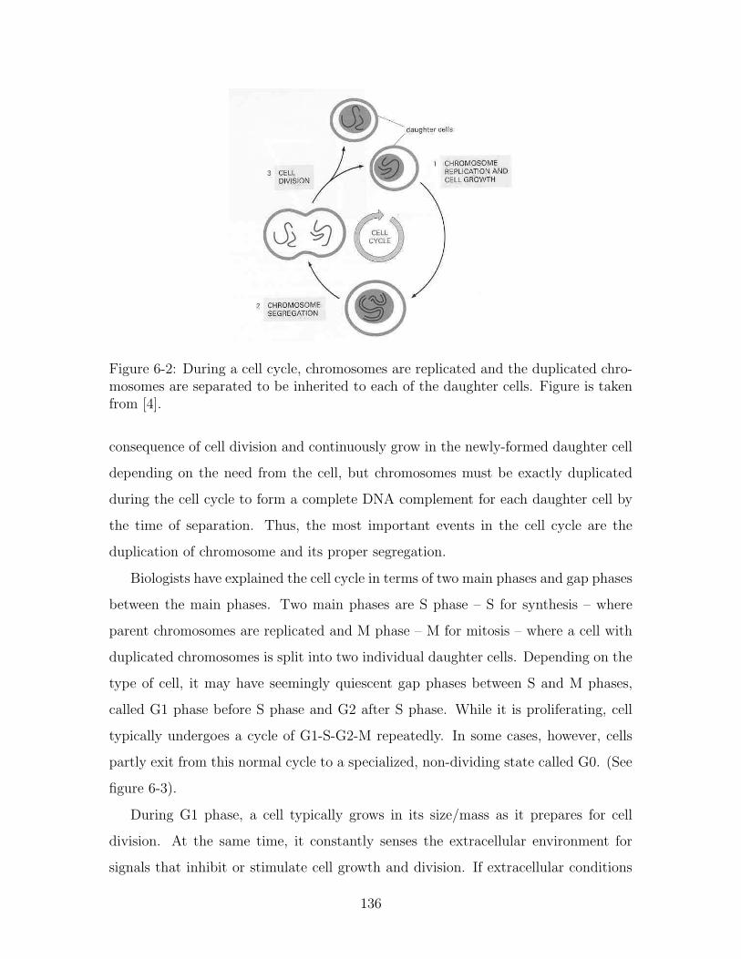
Figure 6-2: During a cell cycle, chromosomes are replicated and the duplicated chro-mosomes are separated to be inherited to each of the daughter cells. Figure is takenfrom [4].

consequence of cell division and continuously grow in the newly-formed daughter cell

depending on the need from the cell, but chromosomes must be exactly duplicated

during the cell cycle to form a complete DNA complement for each daughter cell by

the time of separation. Thus, the most important events in the cell cycle are the

duplication of chromosome and its proper segregation.

Biologists have explained the cell cycle in terms of two main phases and gap phases

between the main phases. Two main phases are S phase – S for synthesis – where

parent chromosomes are replicated and M phase – M for mitosis – where a cell with

duplicated chromosomes is split into two individual daughter cells. Depending on the

type of cell, it may have seemingly quiescent gap phases between S and M phases,

called G1 phase before S phase and G2 after S phase. While it is proliferating, cell

typically undergoes a cycle of G1-S-G2-M repeatedly. In some cases, however, cells

partly exit from this normal cycle to a specialized, non-dividing state called G0. (See

figure 6-3).

During G1 phase, a cell typically grows in its size/mass as it prepares for cell

division. At the same time, it constantly senses the extracellular environment for

signals that inhibit or stimulate cell growth and division. If extracellular conditions

136

S

G1

G2

M

Mitosis (nuclear division)Cytokinesis

(cytoplasmic division) Cell growthExtracellular signalCheckpoint

DNA replicationCell growthCheckpoint

G0

Non-dividing/resting state

Figure 6-3: Cell cycle progresses through different phases: DNA is replicated duringS phase, and the nucleus and cytoplasm divide in M phase. Partly to allow more timefor growth, most cells have gap phase: G1 between M and S phase and G2 between Sand M phase. Depending on the extracellular condition, some cells enter a specializedresting state, called G0.

are favorable and the cell has grown enough, then it commits itself to cell division

process by entering S phase for chromosome duplication. As chromosomes are being

duplicated inside a nucleus during S phase, a microtubule-organizing organelle, called

the centrosome, is duplicated outside the nucleus. Later in M phase, centrosomes play

a crucial role in segregating duplicated chromosomes. Completion of DNA replication

in S phase leads to G2 phase where the cell is getting ready for actual separation.

Then, the cell finally enters M phase. In the first half of M phase, the membrane of

the original nucleus is broken down, and the replicated chromosomes are segregated

and pulled apart to opposite sides of the cell. Then, new nuclear membrane is formed

around each of the two chromosome sets to form two intact nuclei. This process of

nuclear division is called mitosis. Following mitosis is the separation of the parent cell

into two daughter cells each with one nucleus. This process of cytoplasmic division

is called cytokinesis. After cytokinesis, two individual cells are formed and they are

in their G1 phase and proceed to the next round of their own cell cycle.

6.1.2 Regulating the Cell Cycle: Cyclin and Cdk

The progress of cell cycle, e.g. from G1 to S phase, is precisely regulated by the cell

cycle control mechanism. Considering that the correct completion of cell division is

137

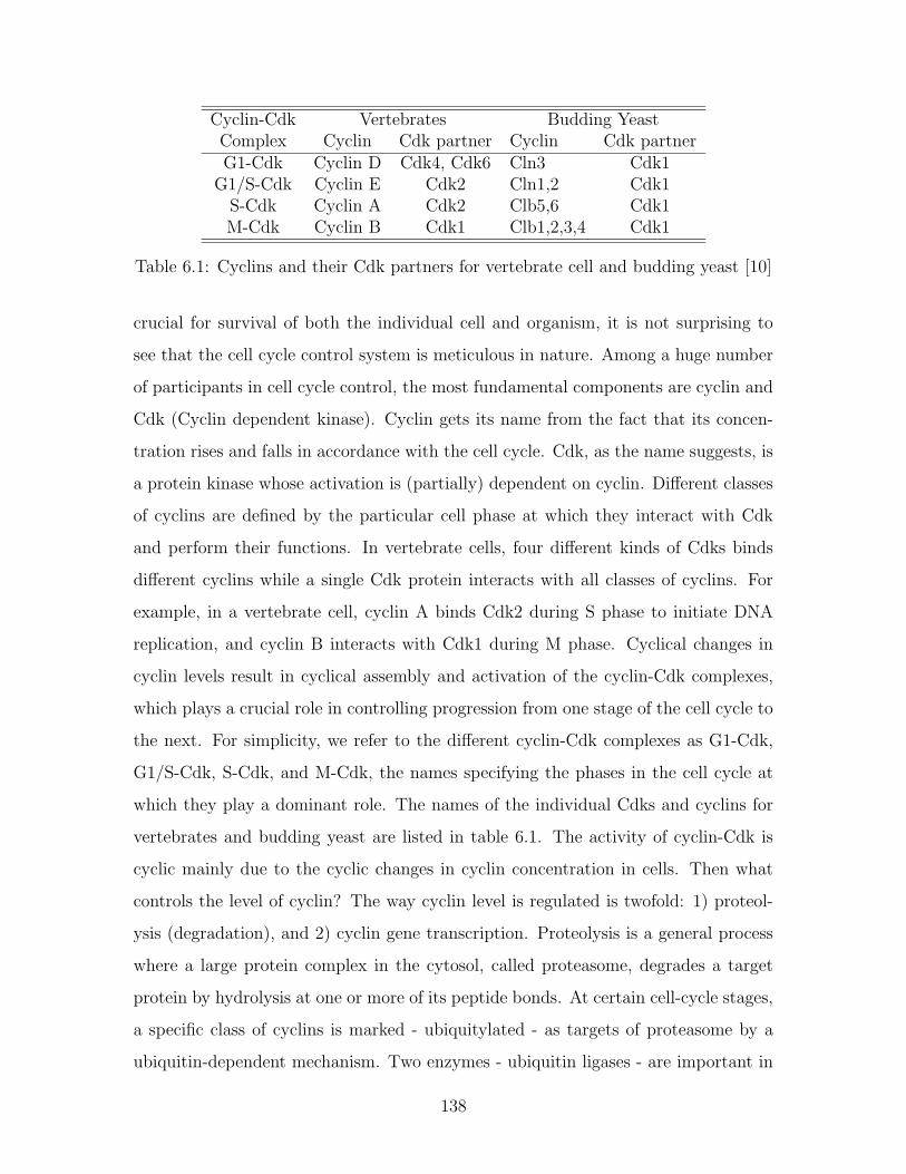
Cyclin-Cdk Vertebrates Budding YeastComplex Cyclin Cdk partner Cyclin Cdk partnerG1-Cdk Cyclin D Cdk4, Cdk6 Cln3 Cdk1

G1/S-Cdk Cyclin E Cdk2 Cln1,2 Cdk1S-Cdk Cyclin A Cdk2 Clb5,6 Cdk1M-Cdk Cyclin B Cdk1 Clb1,2,3,4 Cdk1

Table 6.1: Cyclins and their Cdk partners for vertebrate cell and budding yeast [10]

crucial for survival of both the individual cell and organism, it is not surprising to

see that the cell cycle control system is meticulous in nature. Among a huge number

of participants in cell cycle control, the most fundamental components are cyclin and

Cdk (Cyclin dependent kinase). Cyclin gets its name from the fact that its concen-

tration rises and falls in accordance with the cell cycle. Cdk, as the name suggests, is

a protein kinase whose activation is (partially) dependent on cyclin. Different classes

of cyclins are defined by the particular cell phase at which they interact with Cdk

and perform their functions. In vertebrate cells, four different kinds of Cdks binds

different cyclins while a single Cdk protein interacts with all classes of cyclins. For

example, in a vertebrate cell, cyclin A binds Cdk2 during S phase to initiate DNA

replication, and cyclin B interacts with Cdk1 during M phase. Cyclical changes in

cyclin levels result in cyclical assembly and activation of the cyclin-Cdk complexes,

which plays a crucial role in controlling progression from one stage of the cell cycle to

the next. For simplicity, we refer to the different cyclin-Cdk complexes as G1-Cdk,

G1/S-Cdk, S-Cdk, and M-Cdk, the names specifying the phases in the cell cycle at

which they play a dominant role. The names of the individual Cdks and cyclins for

vertebrates and budding yeast are listed in table 6.1. The activity of cyclin-Cdk is

cyclic mainly due to the cyclic changes in cyclin concentration in cells. Then what

controls the level of cyclin? The way cyclin level is regulated is twofold: 1) proteol-

ysis (degradation), and 2) cyclin gene transcription. Proteolysis is a general process

where a large protein complex in the cytosol, called proteasome, degrades a target

protein by hydrolysis at one or more of its peptide bonds. At certain cell-cycle stages,

a specific class of cyclins is marked - ubiquitylated - as targets of proteasome by a

ubiquitin-dependent mechanism. Two enzymes - ubiquitin ligases - are important in

138

cyclin destruction: SCF and APC. SCF is named after its three main protein sub-

units, and is responsible for the ubiquitylation and destruction of G1/S-cyclin. APC

(Anaphase-promoting complex) is responsible for M-cyclin proteolysis in M phase.

While SCF and APC are one part of cyclin regulation, control of cyclin synthesis is

another important part. Cyclin levels in most cells are controlled not only by changes

in cyclin degradation but also by changes in cyclin gene transcription and thereby cy-

clin synthesis. For example, transcription of genes encoding S cyclins is promoted by

a gene regulatory protein, E2F. Promoted by E2F, increased level of S cyclin synthesis

leads to the increase in S-Cdk activity. Although the details of this gene expression

regulation remain unknown, it is certain that cyclin gene transcription provides an

added level of regulation. In addition to the above primary determinant of cyclic

activation of cyclin-Cdk, there are additional mechanisms involved in Cdk activity

regulation. These mechanisms include CAK (Cdk-activating kinase), inhibitory ki-

nase (e.g. Wee1 kinase), phosphatase (e.g. cdc25) and CKI (Cdk inhibitor protein).

By interacting with cyclin-Cdk complex when called upon, they provide the ability

of fine-tuning Cdk activity in the cell cycle. To summarize, the level of cyclin-Cdk

activity is regulated by the following mechanisms:

• degradation of cyclin: SCF, APC

• synthesis of cyclin: gene transcription control (E2F)

• CAK (Cdk-activating kinase)

• CKI (Cdk inhibitor protein): p27, p21, p16

• Cdk phosphorylation/dephosphorylation: Wee1 inhibitory kinase, Cdc25 acti-

vating phosphatase

• and possibly other mechanisms that are yet to be described

139

6.1.3 Transition of Phases in the Cell Cycle

After the completion of a cell cycle, each of the daughter cells has to have inherited

exactly one copy of chromosome as well as other organelles from their parent cell to

properly function. Therefore, the chromosome replication is among the most critical

events in a cell cycle. This critical event occurs during S phase (S for synthesis),

which requires 10-12 hours and occupies about half of the cell-cycle time in a typical

mammalian cell. The molecular details of the DNA duplication are beyond the scope

of this chapter, and we concentrate on the regulatory mechanism from the cell cycle

control perspective.

The S phase regulatory mechanism has two main functions. One is to initiate

the chromosome replication process, and the other is to prevent it from happening

more than once per cycle. The second task is as important as the first since hyper-

replication of chromosomes results in an abnormal number of genes in one or both

daughter cells and leads to serious damage to the cell itself and potentially the organ-

ism as a whole. Initiation of chromosome duplication requires the activity of S-Cdk.

Chromosome replication begins at “origins of replication.” The origins of replication

are scattered at various locations in the chromosome, and serve as the landing sta-

tions for chromosome replication ‘machine.’ A large, multi-protein complex known as

the origin recognition complex (ORC) binds to the origin of replication. In early G1

phase, the level of Cdc6, one of the regulatory proteins, increases transiently. Cdc6

binds to ORC, and together they promote the formation of Mcm protein rings on the

adjacent DNA, which later migrate along DNA strands. The resulting protein com-

plex, bindings of ORC, Cdc6, and Mcm rings, is known as the pre-replicative complex

(pre-RC). With pre-RC in place, the replication origin is ready to fire. The activation

of S-Cdk in late G1 phase triggers the origin firing, assembling DNA polymerase and

other replication proteins and activating the Mcm protein rings. S-Cdk is also respon-

sible for preventing hyper-replication of chromosome. First, it disassembles pre-RC

by causing the Cdc6 protein to dissociate from ORC after the origin has fired. At

the same time, it phosphorylates Cdc6, which in turn triggers Cdc6 ubiquitylation by

140

the SCF enzyme. As a result, the level of free Cdc6 protein decreases quickly after

the initiation of chromosome replication. S-Cdk also phosphorylate some Mcm pro-

teins. It causes the export of Mcm protein from the nuecleus, and thus enhances the

preventive mechanism. G1/S-Cdk and M-Cdk also helps restraining the unwanted

pre-RC assembly to make sure DNA replication does not occur after S phase. Having

understood that S-Cdk is the key component in progression into S phase, what, then,

activates S-Cdk? Activating S-Cdk requires another set of mechanisms which involve

extracellular signal, and the detail is discussed later.

Having two accurate copies of the entire genome, the cell is (almost) ready to

undergo M phase, where the duplicated chromosomes and other cell contents are

distributed equally to the two daughter cells. M phase is further broken down to

two stages: mitosis and cytokinesis. During mitosis, a series of events occur: the

replicated chromosomes condense, the mitotic spindle assembles, nuclear envelope

breaks down, microtubules attach to the chromosomes, the chromosomes are aligned

at the equator of the cell, the sister chromatids abruptly separate and are pulled

apart, and new nuclear envelopes are formed around each of the chromosome set

completing nuclear division. Once the nucleus is divided, other substances are to be

divided. During cytokinesis, the cytoplasm (extra-nuclear substances) is divided in

two by a contractile ring of filaments, completing the cell division process for one

generation.

M-Cdk is responsible for initiating a number of events during M phase: the repli-

cated chromosomes have to be rearranged for separation, the microtubules have to

be organized around centrosome to form mitotic spindle, the spindles are attached

to the replicated chromosomes, and so on. Once the complex rearrangements of the

chromosomes and mitotic spindle are completed, the sister chromatids are to be sep-

arated. It is not M-Cdk but the anaphase-promoting complex (APC) that triggers

the separation, the most dramatic event in M phase. When duplicated, the two sister

chromatids are bound tightly together by the action of cohesin complex. Active APC

acts on a protein complex that dissociates cohesin from the chromosomes and thereby

initiates the sister chromatids separation. The separation of sister chromatids is im-

141

Figure 6-4: At the end of M phase, the activity of M-Cdk is suppressed by Cdc20-APCand Hct1-APC. Figure is taken from [6].

mediately followed by cytokinesis where cytoplasm is divided into two and thus two

daughter cells are formed.

At the end of M phase when the chromosomes have been completely separated, the

cell reverses the changes to prepare for cytokinesis. The spindle is disassembled, the

chromosomes decondenses, and the nuclear envelope is re-formed. It is believed that

M-Cdk inactivation is mainly responsible for this reversing process, and thus triggers

the exit from mitosis. While Cdc20-APC complex initiates sister chromatids sepa-

ration, it also inactivates M-Cdk by ubiquitylating M-cyclin. Thus, as Cdc20-APC

become more active toward the end of M phase, M-Cdk level decreases. Interest-

ingly, since the activation of Cdc20-APC requires M-Cdk, the activity of Cdc20-APC

also decreases along with M-Cdk level. By this feedback mechanism, the destruction

of M-cyclin leads to the inactivation of APC activity, which then allows the cell to

quickly begin accumulating new M-cyclin for the next cell cycle (see figure 6.1.3). It

is a useful setup for embryonic cells with no G1 phase, but not very useful for cells

with G1 phase because they need to suppress Cdk activity for a while to allow for

cell growth and to be regulated by extracellular signals. Therefore, cells with G1

phase need other mechanisms to ensure that Cdk reactivation is prevented after mi-

tosis. There are three mechanisms that suppress Cdk activity at the end of M phase:

Hct1-APC complex that initiates the ubiquitylation of M-cyclin, CKI accumulation

(Sic1 in budding yeast cell and p27 in mammalian cell), and reduced transcription

of M-cyclin genes. The first two are mutually inhibitory with respect to M-Cdk,

i.e. Hct1-APC and CKI suppress M-Cdk, and vice versa. By this mutual inhibition,

142

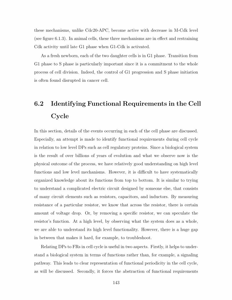
these mechanisms, unlike Cdc20-APC, become active with decrease in M-Cdk level

(see figure 6.1.3). In animal cells, these three mechanisms are in effect and restraining

Cdk activity until late G1 phase when G1-Cdk is activated.

As a fresh newborn, each of the two daughter cells is in G1 phase. Transition from

G1 phase to S phase is particularly important since it is a commitment to the whole

process of cell division. Indeed, the control of G1 progression and S phase initiation

is often found disrupted in cancer cell.

6.2 Identifying Functional Requirements in the Cell

Cycle

In this section, details of the events occurring in each of the cell phase are discussed.

Especially, an attempt is made to identify functional requirements during cell cycle

in relation to low level DPs such as cell regulatory proteins. Since a biological system

is the result of over billions of years of evolution and what we observe now is the

physical outcome of the process, we have relatively good understanding on high level

functions and low level mechanisms. However, it is difficult to have systematically

organized knowledge about its functions from top to bottom. It is similar to trying

to understand a complicated electric circuit designed by someone else, that consists

of many circuit elements such as resistors, capacitors, and inductors. By measuring

resistance of a particular resistor, we know that across the resistor, there is certain

amount of voltage drop. Or, by removing a specific resistor, we can speculate the

resistor’s function. At a high level, by observing what the system does as a whole,

we are able to understand its high level functionality. However, there is a huge gap

in between that makes it hard, for example, to troubleshoot.

Relating DPs to FRs in cell cycle is useful in two aspects. Firstly, it helps to under-

stand a biological system in terms of functions rather than, for example, a signaling

pathway. This leads to clear representation of functional periodicity in the cell cycle,

as will be discussed. Secondly, it forces the abstraction of functional requirements

143

to a higher level which at the same time the top level functional requirements are

decomposed so that the available information is put into context. Also, some of the

unrealized research questions can be raised by examining a system from functional

perspective, which would be hard to do just through the interpretation of observed

mechanisms.

6.2.1 Functional Decomposition for G1 phase

Top level FR-DP

Having understood the state of a cell at the end of M phase, it is not difficult to guess

what needs to happen during G1 phase. It has to constantly monitor signals for cell

cycle progression, and, once it comes, all three Cdk inhibitory mechanisms must be

reversed so that S phase is quickly initiated. As a preparation for chromosome repli-

cation, it also has to form pre-RC during G1 phase. To maintain its size throughout

the successive dividing processes, a typical cell must grow its size. Otherwise, the

size of a cell becomes smaller and smaller as it divides itself. Note, however, in some

cases cell does divide without growing (embryonic development), and grow without

dividing (neuron). Another critical function is that a cell must prevent itself from

entering S phase if there is something wrong with the cell. For example, a cell with

DNA damage should not replicate itself to avoid creating malfunctioning daughter

cells. In summary, the following is a list of functional requirements for G1 phase in

particular relation to cell cycle regulation:

• FR1: Form DNA replication ‘machine’

• FR2: Grow cell to maturity

• FR3: Sense environment to determine the entry to next phase

• FR4: Cause cell cycle arrest/death if necessary

• FR5: Initiate exit-G1 & entry-S

144

Design parameters can be stated for each of the above functional requirements. Albeit

abstract at this level of decomposition, explicitly stating design parameters helps

organizing information into perspective.

• DP1: Pre-RC forming mechanism

• DP2: Extracellular signal (growth factors)

• DP3: Extracellular signal (mitogens)

• DP4: Cell cycle inhibitory mechanism / Apoptosis

• DP5: Rb-pathway

DP1, pre-RC forming mechanism, as discussed in 6.1.3, involves the activities of sev-

eral proteins (e.g. Cdc6, Mcm) and is solely responsible for creating the pre-replicative

complex at the origin of replication on DNA strand. DP2 is the extracellular growth

factor (e.g. PDGF, EGF) , which stimulates cell growth by initiating intracellular

signaling pathway. For single-celled organisms such as yeasts, cell growth depends

only on nutrients. By contrast, animal cells require both nutrients and extracellular

signals typically from other neighboring cells. DP3 is another type of extracellular

substance, called mitogens. It initiates an intracellular signaling pathway, called Rb

pathway, that leads to the break down of the blocking mechanisms that suppress the

progress of cell cycle. Many extracellular signal proteins act as growth factor as well

as mitogen. Also, growth factor stimulation also leads to increased production of the

gene regulatory protein. DP4 is responsible for monitoring the anomaly in cell activ-

ity and taking appropriate action if necessary. This is very important FR-DP pair in

regulating cell reproduction and suppressing cancer development, and the failing of

this FR-DP is indeed commonly found in cancer cells. FR5 is the ultimate outcome

of normal G1 phase, and Rb-pathway delivers the function.

The top level FR-DP pairs are decomposed to the next level to describe the system

with further detail.

145

Decomposition of FR1-DP1: pre-RC forming mechanism

FR1-DP1 (pre-RC development) is decomposed to:

FR11: Mark origin of duplication DP11: ORC - origin interaction

FR12: Create Mcm helicase ring DP12: Cdc6-dependent mechanism

As discussed in background section, pre-RC creation requires ORC-origin interaction

to mark the origin location. It is a stable interaction that marks a replication origin

throughout the entire cell cycle. On the contrary, Cdc6-dependent mechanism is

cell cycle dependent: Cdc6 is present at low levels during most of the cell cycle but

increases transiently in early G1. Transcription of this protein was reported to be

regulated in response to mitogenic signals through transcriptional control mechanism.

Decomposition of FR2-DP2: Response to extracellular growth factors

FR2-DP2 (growth factors) has the following sub FRs-DPs:

FR21: Detect growth factor DP21: Growth factor receptor

FR22: Stimulate protein synthesis DP22: Growth factor pathways

FR23: Suppress cell cycle until it grows

enough

DP23: G1-cyclin inhibitory mecha-

nism

To grow the cell, it has to increase the level of protein synthesis. This requires in-

creased mRNA transcription and mRNA translation, which are stimulated by growth

factors. For example, PI 3-kinase activates the S6 protein kinase and a translation

initiation factor called eIF4E, which leads to increased mRNA translation. Most

of these mRNA encode ribosomal components and as a result, protein synthesis in-

creases. Since the exit from G1 phase begins by G1-cyclin accumulation, for a cell to

have enough time to grow, it needs to suppress the available G1-cyclin level. DP23,

G1-cyclin inhibitory mechanism is responsible for the function. It is quite interesting

that G1-cyclin that is an important factor in determining dell division timing also

holds an important role in cell growth regulation. For a cell that grows and divides,

146

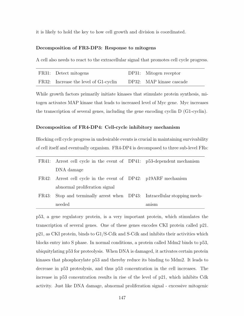
it is likely to hold the key to how cell growth and division is coordinated.

Decomposition of FR3-DP3: Response to mitogens

A cell also needs to react to the extracellular signal that promotes cell cycle progress.

FR31: Detect mitogens DP31: Mitogen receptor

FR32: Increase the level of G1-cyclin DP32: MAP kinase cascade

While growth factors primarily initiate kinases that stimulate protein synthesis, mi-

togen activates MAP kinase that leads to increased level of Myc gene. Myc increases

the transcription of several genes, including the gene encoding cyclin D (G1-cyclin).

Decomposition of FR4-DP4: Cell-cycle inhibitory mechanism

Blocking cell cycle progress in undesirable events is crucial in maintaining survivability

of cell itself and eventually organism. FR4-DP4 is decomposed to three sub-level FRs:

FR41: Arrest cell cycle in the event of

DNA damage

DP41: p53-dependent mechanism

FR42: Arrest cell cycle in the event of

abnormal proliferation signal

DP42: p19ARF mechanism

FR43: Stop and terminally arrest when

needed

DP43: Intracellular stopping mech-

anism

p53, a gene regulatory protein, is a very important protein, which stimulates the

transcription of several genes. One of these genes encodes CKI protein called p21.

p21, as CKI protein, binds to G1/S-Cdk and S-Cdk and inhibits their activities which

blocks entry into S phase. In normal conditions, a protein called Mdm2 binds to p53,

ubiquitylating p53 for proteolysis. When DNA is damaged, it activates certain protein

kinases that phosphorylate p53 and thereby reduce its binding to Mdm2. It leads to

decrease in p53 proteolysis, and thus p53 concentration in the cell increases. The

increase in p53 concentration results in rise of the level of p21, which inhibits Cdk

activity. Just like DNA damage, abnormal proliferation signal - excessive mitogenic

147

stimulation - causes p53 activation. The abnormal proliferation signal leads to the

activation of cell-cycle inhibitor protein called p19ARF, which binds and inhibits

Mdm2 resulting in p53 increase. DP43, stopping mechanism, is poorly understood.

One possible explanation is a progressive increase in CKI p27. Another is ‘replicative

cell senescence (aging)’ by a pair of sub-mechanisms.

Decomposition of FR5-DP5: Rb-pathway

Before decomposing FR5-DP5, examining the signaling pathway first will help un-

derstand the sublevel functional requirements. Recall that at the end of M phase,

three Cdk-inhibitory mechanisms are in effect: low level of cyclin gene transcription,

Hct1-APC, and CKI (p27 for mammalian cells), which collectively prevent Cdk ac-

tivity. The activation of G1-Cdk is the very first step to reverse all three inhibitory

mechanisms. The phosphorylation target of active G1-Cdk is retinoblastoma protein

(Rb), an inhibitor of cell-cycle progression. During G1 phase, Rb binds to a gene reg-

ulatory protein called E2F and inhibits E2F activity. E2F promotes transcription of

many genes that encode proteins required for S-phase entry such as G1/S-cyclins and

S-cyclins. Thus, G1-Cdk with E2F as mediator stimulates the synthesis of G1/S-Cdk

and S-Cdk. Then, what about those Cdk-inhibitory mechanisms? As with M-Cdk,

G1/S-Cdk and S-Cdk also form positive feedback loops. The increase in these Cdk ac-

tivities enhances the phosphorylation of Hct1 and p27, leading to their inactivation or

destruction. Therefore, activation of G1/S-Cdk and S-Cdk result in more activation

of themselves. Two more feedback loops enhance the process. Active E2F promotes

the transcription of its own gene. G1/S-Cdk and S-Cdk enhance phosphorylation

of Rb and thereby promote E2F release, which then increases gene transcription of

G1/S-cyclin and S-cyclin. These enhancing feedback mechanisms ensure the rapid

transition from G1 phase to S phase, once initiated by G1-Cdk.

The remaining part of the G1-S phase transition mechanism is G1-Cdk activation.

In animal cells, activating G1-Cdk requires stimulation by the extracellular signals.

As discussed in FR3-DP3 decomposition, mitogens promote the gene transcription

for G1-cyclin. Not only does mitogen-dependent mechanism stimulate G1-cyclin syn-

148

G1-Cdk

Mitogen-dependentmechanism

(Extracellular signal)

genetranscription

G1/S-cyclin

S-cyclin

Rb

E2F

CKI:p27

G1/S-Cdk

S-Cdk

Hct1-APC

promoteaccumulation

inactivate

inactivate

inactivate

mutuallyinhibits

inactivate

mutuallyinhibits

mutuallyinhibits

Figure 6-5: G1-Cdk triggers the phase transition from G1 to S by initiating a seriesof events that lead to increased level of S-Cdk activity.

thesis, but it also helps the transition by additional activities. The regulatory protein

Myc increases the transcription of genes including a gene encoding a subunit of the

SCF enzyme and E2F gene as well as G1-cyclin gene. SCF enzyme ubiquitylates CKI

p27, leading to the increase in G1/S-Cdk activity. Increased level of E2F protein

by transcription of E2F gene promotes its own gene transcription. The end result

of the whole mechanism is the increased S-Cdk activity and consequently exit from

G1 phase. Figure 6-5 shows the overall signaling pathway involved in G1-S phase

transition. FR-DP representation of the above mechanism is shown below:

FR51: Accumulate G1-Cdk DP51: Available G1-cyclin

FR52: Inactivate Rb DP52: G1-Cdk

FR53: Promote E2F synthesis DP53: Rb phosphorylation

FR54: Promote S-cyclin synthesis DP54: E2F

FR55: Activate S-Cdk DP55: S-cyclin

FR56: Inactivate CKI (p27) DP56: G1/S-Cdk

FR57: Inactivate Hct1 DP57: S-Cdk

FR58: Promote G1/S-cyclin synthesis DP58: E2F

FR59: Activate G1/S-Cdk DP59: G1/S-cyclin

149

OR

C-o

rigin

inte

ract

ion

cdc6

mec

hani

sm

Gro

wth

fact

or r

ecep

tor

Ext

race

llula

r gr

owth

fact

or p

athw

ay

Cln

3 in

hibi

tory

mec

hani

sm

Mito

gen

rece

ptor

Myc

(ge

ne r

egul

ator

y pr

otei

n)

p53-

depe

nden

t mec

hani

sm

p19A

RF

->p5

3 m

echa

nism

Intr

acel

lula

r st

oppi

ng m

echa

nism

Ava

ilabl

e G

1-C

yclin

G1-

Cdk

Inac

tivat

ion

of R

b

E2F

S-c

yclin

G1/

S-C

dk

S-C

dk

G1/

S-c

yclin

Mark origin of duplication XForm Mcm helicase X 13 13 16 16Detect growth factor XStimulate cell growth 15 X 3Suppress cell cycle until grows enough 1 X cDetect mitogen 14 2 XIncrease the level of G1-Cyclin b 4 XArrest cell cycle in the event of DNA damage X O**Arrest cell cycle in the event of abnormal proliferation signals d 5 XStop and terminally arrest XAccumulate G1-Cdk O* b 6 XInactivate Rb f XPromote E2F protein 7 g X 11Promote S-phase gene transcription h XActivate 'some' of S-Cdk 9 9 k XInactivate CKI (e.g. Sic1, p27) 8 X 12Deactivate Hct1 (APC-activating protein) 12 XActivate 'some' of G1/S-Cdk 10 10 m X

Figure 6-6: Design matrix for FR-DP in G1 phase

Design matrix

Now that we have fair details on the functional requirements and design parameters,

a design matrix is constructed to examine the interrelationship among FRs and DPs.

The design matrix is shown in figure 6-6, and the explanations on each of non-zero

design matrix elements are given as numbered annotation. Since the interactions

indicated by diagonal elements (marked by ’X’) are self explanatory, only the off-

diagonal elements - cross interactions - are explained. Off-diagonal elements labeled

with numbers indicate strong interactions, whereas alphabetic labels imply relatively

weak interrelationships. Two of the zero elements are also explained for clarity. Note

that the symbol ‘A→ B’ means that A activates or increases the activity of B, whereas

‘A a B’ means inactivation or suppression of B by A.

1. G1-cyclin is synthesized in proportion to cell growth

2. Many extracellular growth factors activate the signaling protein Ras,

which stimulates the MAP-kinase pathway to trigger cell-cycle progression

150

3. Many mitogens stimulate cell-growth by Mitogen→ Ras→ PI3-kinase

4. Mitogen→ Ras→MAP-kinase→Myc→ G1-cyclin gene transcription

5. Excessive Myc production induces cell-cycle arrest

6. Myc → G1-cyclin transcription → G1-cyclin → G1-Cdk

7. Myc → E2F transcription → E2F

8. Myc → SCF subunit transcription → SCF → p27 degradation

9. p53 → p21 transcription → p21 CKI a S-Cdk

10. p53 → p21 transcription → p21 CKI a G1/S-Cdk

11. E2F → E2F transcription

12. Symmetry: S-Cdk&G1/S-Cdk a Hct1-APC&CKI

13. Creating Mcm-halicase requires Cdc6 which in turn is regulated in

response to mitogenic signal through transcriptional control mechanism

involving E2F proteins.

14. Many growth factor receptors also recognize mitogens.

15. Receptor → Ras → PI 3-kinase

16. G1/S-Cdk and S-Cdk prevents Mcm ring formation after S phase

initiation to prevent multiple DNA replication

a. Excessive Myc production induces cell-cycle arrest

b. G1-cyclin inhibitory mechanism poses a threshold level for G1-cyclin

c. Myc promotes G1-cyclin synthesis (Indeed, ’1’ is rather (3,3)-2-(5,5)-

4-(6,6)-c )

d. Excessive Myc production induces cell-cycle arrest

f. G1-cyclin → G1-Cdk a Rb

g. G1-Cdk a Rb a E2F

O*. Extracellular GF eventually contributes to G1-Cdk accumulation by

GF → Ras → MAP-kinase → Myc → G1-cyclin → G1-Cdk. However,

151

that is too far-downstream, and that effect is represented by a chain DP21

→ FR32 → DP32 → FR41

O**. p19ARF leads to p53 mechanism, but has nothing to do with DNA

damage

Apparently, the above full design matrix looks like a coupled design matrix. Given

that the cell cycle is successfully managed repeatedly in normal multicellular organ-

isms, having a coupled design matrix may be explained by one of the following possi-

ble reasons. First, cells have evolved to have coupled relationships, but the cell cycle

regulatory mechanism has been able to somehow manage the coupled relationships.

If that is true, the cell cycle regulatory mechanism must involve intensive feedback

mechanisms and they have to be tightly controlled. In other words, the existence of

coupled design matrices is an evidence of complicated regulatory mechanism. Sec-

ond, although it looks coupled at this level of decomposition, it is indeed a decoupled

design if further decomposed. A theorem that addresses such a peculiarity was pro-

posed by Melvin [26], and that may be the case with this design matrix. Thirdly,

there is a possibility that the information captured by this design matrix is incorrect

or incomplete because much of the details about the cell regulatory mechanisms are

unknown yet. Testing each of the three hypotheses is an interesting problem from

both cell biology and axiomatic design perspective.

6.3 Centrosome Cycle

The previous section discussed the cell cycle mainly from the perspective of the chro-

mosome cycle. It focuses on the functional requirements to duplicate chromosomes

and divide the replicated chromosomes into two daughter cells. As part of M phase

FR-DP decomposition, the function of centrosome is briefly mentioned. While it

is a part of chromosome cycle, centrosome has its own functional cycle for duplica-

tion and it is independent of the chromosome cycle in that the centrosome cycle can

progress independent of chromosome cycle. This section discusses centrosome cycle

and importance of maintaining synchronized periodicity between two cycles.

152

Prophase Prometaphase MetaphaseProphase Prometaphase Metaphase Anaphase TelophaseAnaphase Telophase

Figure 6-7: During mitosis, nuclear division, centrosomes shown as circles in thisfigure play an important role as microtubule-organizing center. Figure is taken from[7].

6.3.1 Centrosome: Microtubule Organizing Center

During mitosis, sister chromatids (duplicated chromosomes) are separated and pulled

apart from each other to the opposite side of a cell. The mitotic spindle, an array of

microtubules, performs the action of separating sister chromatids. Although in cells

of higher plants and in many meiotic cells, bipolar spindles are assembled without

centrosomes, in most animal cells, centrosome is known to play an important role

in organizing microtubules to form the mitotic spindle [43],[44]. As a microtubule

organizing center, the centrosome takes central stage during mitosis. Microtubules

are nucleated within centrosome, and centrosome acts as a pole. As a nucleation site

and mitotic spindle pole, it coordinates the microtubule activity during M phase.

Figure 6-7 shows a series of events during mitosis. In early M phase, each of a

pair of centrosomes moves toward the opposite side of the cell, forming mitotic spindle

poles at each side. As nuclear envelope breaks down, one end of mitotic spindle is

attached to a sister chromatid’s kinetochore while the other end is anchored at the

spindle pole. Once the kinetochores on both sides of sister chromatids are attached

to microtubules, the chromosome is said to have formed bipolar mitotic spindle at-

tachment. By the action of attached mitotic spindle, the replicated chromosomes are

aligned along a plane, called metaphase plate, that is nearly equidistant between the

two spindle poles. With each of the centrosomes as a pole, kinetochore microtubules

– microtubules that are attached to kinetochore – shrinks in length. Shortening of

the length of kinetochore microtubules creates a pulling force that separates sister

chromatids. Although the bipolar spindle may be formed without centrosomes in

153

Figure 6-8: The centrosome consists of a pair of centrioles, surrounded by pericentri-olar material. Lines in the figure are microtubues nucleated and anchored at pericen-triolar material.

vertebrate cells whose centrosomes have been destroyed with a laser beam, the spin-

dle is often mispositioned, resulting in abnormalities in cytokinesis [6].

The centrosome consists of a pair of centrioles, pericentriolar material (sometimes

called pericentriolar matrix), and centrosomal domain (See figure 6-8). The centriole

is a barrel-shaped, cylindrical organelle that is found in most animal cells. Although

the functions of the centrioles within the centrosome remain unclear, centrioles are be-

lieved to be important in the assembly of pericentriolar material and the stabilization

of the centrosomal structure [45],[46],[8]. Also, since centrosomes lacking centrioles

do not reproduce in animal cells, centrioles seem to play an important role in centro-

some reproduction [45]. The centriole pair is oriented perpendicular to each other,

but the significance of this unusual orientation is still unknown [47]. Pericentriolar

material surrounds the centrioles, and contains elements that nucleate and organize

microtubules. Most importantly, it contains γ-tubulin complex that seems to serve as

a template for microtubule polymerization. Instead of having a clearly defined bound-

ary, the centrosomes extend out and integrate with cytoplasm, and these extensions

are called outer centrosomal domain.

As a normal vertebrate cell enters M phase, a cell contains a pair of duplicated

chromosomes and a pair of centrosomes. Thus, a cell has to duplicate exactly one copy

of the existing centrosome prior to M phase. Duplication of centrosome begins with

a separation of a centriole pair and forming a new daughter centriole from mother

154

centrioles. Like chromosome replication, the centrosome is duplicated through a series

of cyclic events, and the process is called centrosome cycle.

6.3.2 The Centrosome Cycle

Centrosome has its own cycle for its duplication. Normally, a single centrosome in a

cell in G1 phase is duplicated exactly once to provide two centrosomes to form the

poles of the mitotic spindle. Duplication of the single centrosome is initiated at the

G1/S transition and completed before mitosis. At mitosis, the duplicated centrosomes

are pulled apart to the opposite side of a cell, and plays a role of the mitotic spindle

poles. When a cell is divided into two daughter cells at the end of M phase, each

daughter cell receives one centrosome, and the centrosome begins its next cycle of

duplication.

Figure 6-9 shows the centrosome cycle. Centrosome cycle begins with a loss of

orthogonal connection between centrioles in a process called centriole disorientation.

Once the centrioles are disoriented and exist as individual centrioles, a new daughter

centriole is formed near one end of of parental centriole, and the nucleated daughter

centriole is called a procentriole. Procentrioles then elongate until they reach full

length. During the next round of duplication, both the the parental centriole and

the daughter centriole from the current generation become parental centrioles for the

next generation. Hence, one of the duplicated centrosomes is ’old’, i.e. containing the

oldest of the four centrioles, and the other is ’young.’ While there exist two centriole

doublet, the duplicated centrosomes remain associated until the cell enters M phase

as indicated by the continuous pericentriolar material in figure 6-9 [47],[8]. In ‘young’

centrosome side, the parental centriole acquires a structure called distal appendages

and cenexin. At the same time, pericentriolar material around young centrosome

grows and acquires ε-tubulin that is initially present only in the old centrosome. As

the cell enters M phase, the centrosomes are finally separated and move away to form

mitotic spindle poles at the opposite side of the cell.

Despite its early discovery as old as late 19th century, research on centrosomes

was not actively pursued except the work in early 20th century by Theodor Boveri

155

Figure 6-9: The centrosome is duplicated during S phase and separated later in Mphase to organize activities of microtubules. Each of the two daughter cells receiveone copy of the centrosomes. Figure is taken from [8].

[45]. It has been actively pursued only recently, sparked mainly by the demonstration

that centrosomal abnormalities are frequent in many common cancers [8]. Centro-

some research is now being extended to a molecular level, and yet much less is known

about centrosome cycle relative to the fair amount of knowledge about chromosome

duplication cycle. It was discovered several years ago that G1/S-Cdk and S-Cdk at

the G1-S phase transition of the cell cycle allows centrosome duplication to proceed

[48],[49],[50]. The earliest step that fails in the absence of Cdk2 activity is disorien-

tation (splitting) of the centrioles [8],[48]. One of the downstream targets of Cdk2

activity is the protein nucleophosmin (NPM/B23). The work by Okuda et al[51] sug-

gests that the protein nucleophosmin is associated with the centrosome during mitosis

and needs to be removed to allow splitting of the centrioles. This explains the link

between Cdk2 activity and the first step of centrosome cycle. Once the centrioles are

split, new daughter centriole, procentriole, is nucleated. Although the regulation of

new centriole formation is not well understood yet, a couple of mechanisms are known

to play an important role in the process, including CaMK II (calmodulin-dependent

156

kinase II)[52] and zyg1 [53]. The procentrioles continue to grow to maximum length

in parallel with the growth of pericentriolar material. With fully grown pair of centro-

some, the last step of centrosome cycle is centrosome separation. It seems that there

is a linkage between duplicated centrosome. A protein kinase, Nek2, along with its

phosphorylation target C-Nap1, seem to regulate the linkage. Other factors that are

likely to be part of the mechanism include a protein CP110, a ubiquitin-conjugating

machine SCF complex, kinase Mps1p, and p53/p21 pathway. As mentioned earlier,

understanding of centrosome cycle regulation is still at its early stage, and involves

many unknowns. Yet, the most important and interesting fact about centrosome

cycle is that its regulation, particularly synchronization with chromosome cycle, is

crucial in maintaining cell’s normality.

6.4 Synchronization of Centrosome Cycle and Chro-

mosome Cycle

Because of the way centrosomes work during mitosis, it is crucial to have exactly one

pair of centrosomes during M phase. Having two properly separated centrosomes at

early M phase is required for a precise division of chromosomes. If there are more

than two centrosomes (the extras called supernumerary centrosomes), missegrega-

tion of chromosomes is likely. Supernumerary centrosomes may produce multipo-

lar spindles unless they fortuitously coalesce into a bipolar spindle. On the other

hand, a single centrosome can induce formation of monopolar spindles. Multipolar

or monopolar spindles do not properly direct cell division and generally provoke ab-

normal segregation of chromosomes [45]. The missegregation of chromosomes results

in the aneuploidy (see figure 6-10), which, in most cases, leads to cell death due to

the lack of essential chromosomes. However, some cells manage to function with de-

fective chromosomes and rarely can acquire an advantage in terms of cell growth. In

fact, aneuploidy is the most prevalent form of genetic instability found in cancer cells.

Recent evidence argues that aneuploidy is a discrete event that contributes to malig-

157

Figure 6-10: Missegregation of chromosomes results in incorrect number of chromo-somes in daughter cells.

Figure 6-11: Centrosomal abnormalities are common in human tumor cells: Tumorcolon tissues(b) contains amplified centrosomes compared to normal cells(a), indicatedby bright spots; Human prostate tumor(d),(e) has multipolar spindles shown by darkspots while normal cell(c) has a bipolar spindle. Images are taken from [8].

nant transformation and tumor progression [45]. As mentioned above, it has long been

recognized that errors in centrosome replication may be an important cause of aneu-

ploidy and might thus contribute to cancer formation [45]. Centrosome abberation is

common to most cancer types. Indeed, extra copies of centrosomes (supernumerary

centrosomes) have been described for nearly all cancers that have been surveyed [8].

For example, figure 6-11 clearly shows centrosomal abnormalities in human tumors.

Figure 6-11(a) and (b) are normal and tumor colon tissues from the same patient.

Bright spots in the figure indicate centrosomes. The tumor cells contains amplified

158

centrosomes that are larger and more numerous than those in the normal tissue. That

is also the case with a human prostate tumor (figure 6-11 (d),(e)). While a normal

cell has bipolar spindle indicated by two dark spots, there are multipolar spindles

in dividing tumor cells. Although it is still being debated whether the centrosomal

abnormality is the cause or consequence of cancer, there is no doubt that the two

phenotypes enhances each other; centrosome aberrations will foster chromosome mis-

segregation, regardless of whether they arose through deregulation of the centrosome

cycle or as a consequence of another primary event [8].

To ensure that there are exactly two centrosomes at the beginning of M phase,

synchronizing the chromosome cycle with centrosome cycle is critical. Figure 6-12(a)

compares two cycles. In normal cells, exactly one copy of chromosomes is replicated

during S phase, and at the same time, exactly one copy of centrosomes is duplicated.

Thereby, by the time of G2-M transition, a cell contains a pair of duplicated chro-

mosomes and centrosomes. That, in turn, ensures daughter cells receive one set of

chromosomes along with one centrosome. If the coordination of the two cycles fails, it

will lead to a change in ploidy. The coordination of these two subsystem cycles has an

interesting similarities with manufacturing system example (see figure 6-12(b)): the

integration of the two subsystems requires precise synchronization of the periodicity

of the two sub-cycles for a proper functioning of the overall system. By recognizing

the analogy, we can view the cell division cycle based on what is learned from the the

manufacturing system scheduling example, i.e. periodicity. We can pose questions

such as what controls the periodicity, what is the re-initialization agent? Do we have

a control over the agent? Answers to these questions are at least partially available

from current knowledge. The two cycles are independent in a sense that these two

cycles can be dissociated at least experimentally during the rapid early nuclear di-

visions in the embryos of some species [54]. In human somatic cells, however, they

were shown to be closely synchronized through the activity of Cdk2. As discussed

in section 6.1.3 and 6.3.2, Cdk2 is known to act as a signal to trigger centrosome

duplication as well as DNA replication at G1-S transition. This ensures one level of

coordination between these two cycles by making the two cycles begin at the same

159

Chromosome cycleCentrosome cycle � �

��

IN Inter-face

Machine Y

MachineX

(a) (b)

Chromosome cycleCentrosome cycle � �

��

IN Inter-face

Machine Y

MachineX

� �

��

IN Inter-face

Machine Y

MachineX

(a) (b)

Figure 6-12: (a) A schematic comparison of centrosome cycle and chromosome cycle.This figure is taken from [8]. (b) Coordination of two cycles bears resemblance to themanufacturing system example presented in chapter 5.

time. Another part of synchronization is related to completing the duplication of

both chromosomes and centrosomes before the cell cycle proceeds to mitosis. For

the chromosome cycle, there is a dedicated mechanism responsible for monitoring the

completion of chromosome replication, which is called a DNA replication checkpoint.

It would be reasonable to expect that there is also a mechanism for centrosome cy-

cle to ensure the completion of the centrosome duplication process. However, such

a mechanism has not been identified yet. Instead, there is an indirect mechanism

during mitosis of the cell cycle that monitors, in some sense, the completion of both

cycles. It is called a spindle attachment checkpoint. At early mitosis, it prevents

further cell cycle progress until all the chromosomes are properly attached to mitotic

spindle. As you can imagine, though, it is unable to directly detect the number of

centrosomes. Thus, the lack of dedicated monitoring mechanism for centrosome du-

plication seems to be one of the reasons for centrosomal abnormality. Finally, after

mitosis and cytokinesis, both chromosome and centrosome cycles must return to their

initial states so that newly-generated daughter cells begin their cell cycle with the

same state. That portion of synchronization is ensured by the three Cdk-inhibitory

mechanisms discussed in 6.1.3. The Cdk-inhibitory mechanism brings the activity

160

Cdk2 (S-Cdk)

Firing origin ofreplication

Centriolesplit

Replicating DNADuplicate

centrosome

Check for completionof DNA replication

Check forcompletion

Prophase

Prometaphase

Metaphase

Check forspindle

attachment

Cen

tro

som

ed

up

licat

ion

Ch

rom

oso

me

du

plic

atio

n

Anaphase

TelophaseCytokinesis

Cdk2 initiates both cycle ensuring one level of synchronization

DNA replication checkpoint ensures completion of chromosome duplication

Centrosome cycle lacks a mechanism to check its completion

G1-Cdk



genetranscription

G1/S-cyclin

S-cyclin

Rb

E2F

CKI:p27

G1/S-Cdk

S-Cdk

Hct1-APC

promoteaccumulation

inactivate

inactivate

inactivate

mutuallyinhibits

inactivate

mutuallyinhibits

mutuallyinhibits

Cdk-inhibitory mechanism

Rb-pathway

Cdk2 (S-Cdk)

Firing origin ofreplication

Centriolesplit

Replicating DNADuplicate

centrosome

Check for completionof DNA replication

Check forcompletion

Prophase

Prometaphase

Metaphase

Check forspindle

attachment

Cen

tro

som

ed

up

licat

ion

Ch

rom

oso

me

du

plic

atio

n

Anaphase

TelophaseCytokinesis

Cdk2 initiates both cycle ensuring one level of synchronization

DNA replication checkpoint ensures completion of chromosome duplication

Centrosome cycle lacks a mechanism to check its completion

G1-Cdk



genetranscription

G1/S-cyclin

S-cyclin

Rb

E2F

CKI:p27

G1/S-Cdk

S-Cdk

Hct1-APC

promoteaccumulation

inactivate

inactivate

inactivate

mutuallyinhibits

inactivate

mutuallyinhibits

mutuallyinhibits

Cdk-inhibitory mechanism

Rb-pathway

Figure 6-13: Synchronization of chromosome and centrosome cycles involve at leastthree mechanisms: S-Cdk acting as a signaling agent to initiate both cycles at thesame time, checkpoints to ensure the completion of duplication process in both cycles,and Cdk-inhibitory mechanism to initialize the level of Cdk at the end of the cell cycle.

level of Cdk to zero, and thus re-initializes the cell cycle (and the subcycles) in terms

of Cdk state. The level of Cdk activity turns into active state as the new cells pre-

pares for the next round of division. Stimulated mainly by extracellular signals, the

active Rb-pathway results in the increased level of S-Cdk. Figure 6-13 summarizes

the coordination activity of a cell. Yet, details of these coordination mechanism is

subject to further research, and it is likely to hold a key to identifying the causality

between centrosomal abnormality and cancer development.

Centrosomal abnormality and resulting aneuploidy is a consequence of the break-

down of synchronized periodicity in chromosome-centrosome cycle. For example,

overduplication of centrosomes within a single chromosome cycle has been proposed

as one scenario. In most cases, this results in fatality in individual cells. Cells with

genetic instability die or at least are not allowed to duplicate. But, rarely a few cells

with genetic instability manage to survive. When they survive, some of them gain an

unregulated periodicity. They proliferate and grow abnormally, which threatens the

161

life of the organism. This shows a quite interesting similarity to the manufacturing

system example discussed in chapter 5. In the scheduling example, a disturbance from

one of the subsystems breaks down the inherent periodicity of the system. Because

of the loss of periodicity, the system eventually yields suboptimal performance of the

system. In case of cell, it leads to death of cell itself, even worse, death of organism

due to cancer.

6.5 Summary

A cell under a microscope presents apparent morphological cycle, and the visually

cyclic events has long been recognized for more than a century. Essential functions

of the cell cycle are faithful replication of chromosomes and precise distribution of

duplicated chromosomes to two daughter cells. Chromosomes are replicated during

S phase, and they are divided into two daughter cells in M phase. G1 and G2 phases

are common for cell growth and regulatory purpose. The progress of cell cycle is

precisely regulated by intricate cell cycle control mechanism. The cell cycle control

mechanism is in charge of ensuring the exactly one copy of chromosome is inherited to

next generation by the end of each cell cycle. Thus, the essence of cell cycle regulatory

mechanism is precise initiation and termination of functional requirements throughout

the cycle.

FR-DP decomposition for G1 phase was presented to demonstrate the utility of

axiomatic design approach in describing and understanding a biological system. First

of all, by identifying and abstracting functions into a hierarchy, it can obscure molec-

ular details for simplicity and clarity. Secondly, it reveals and highlights hidden FRs,

DPs and their interactions. During the process of decomposition, it is required that all

FRs be identified and corresponding DPs be specified along with interrelationships.

Thus, an ambiguity related to any of those will stand out and requires attention.

Lastly, by examining design matrix, it is possible to pose some hypotheses, and test-

ing such hypotheses is an interesting problem from both cell biology and axiomatic

design perspective.

162

Centrosome is known to play an important role as a microtubule organizing center

in successful division of duplicated chromosomes. Centrosome is one of the two or-

ganelles – chromosome being the other – known to replicate exactly once during cell

reproduction. Centrosome has its own duplication cycle which is independent from

chromosome cycle. Coordination of these two cycles is crucial to produce normal

daughter cells for next generation. Failure to synchronize the two cycles results in

the breakdown of regular periodicity of the cell cycle, and leads to a genetic insta-

bility, aneuploidy. Aneuploidy, the abberation in chromosome number is commonly

found in many cancer cells, and is believed to be one of the causes of cancer devel-

opment. This example supports the periodic/combinatorial complexity argument in

axiomatic design’s complexity theory. To maintain periodicity is an important func-

tional requirement in the cell division cycle rather than periodicity being a result or

reflection of something else. By achieving periodicity, cells are able to manage the

level of complexity for their survival. In addition, coordinating centrosome cycle and

chromosome cycle is analogous to integrating multiple subsystems to form a manu-

facturing system that was discussed in chapter 5. By recognizing the analogy, it is

possible to examine the problem with a new perspective. For example, what are the

re-initializing signals, does either of the two cycles re-initialize the other, does the lack

of monitoring mechanism for the completion of centrosome cycle explain the cause of

aneuploidy? This type of new ways of looking at the problem can contribute to the

study of biological systems.

163

Chapter 7

Geometric Periodicity in Designing

Low Friction Surface

Previous two chapters present examples to discuss functional periodicity. Functional

periodicity is considered in temporal domain in that it primarily deals with pattern of

functional requirements’ emergence. This chapter demonstrates periodicity concept in

geometric domain using an example from the field of tribology. Design of low friction

surface discussed by Suh [29] is presented as an example. As briefly mentioned in

the example 4-1, in designing low friction surface, periodic complexity is achieved by

establishing geometric periodicity at the sliding interface.

7.1 Background: Mechanism of Friction

When two surfaces slide against each other, the relative tangential motion is resisted

by some force. The force resisting tangential motion is the frictional force. The

frictional force depends on many factors such as normal load, surface roughness, and

materials of the sliding surfaces. All of these factors except normal load is lumped

into a characteristic parameter, friction coefficient. Although a simple description of

friction force, Ffriction = µN , has practical utility, the actual mechanism that cause

frictional force is quite complicated. Friction at the sliding interface of metals is

caused by the collective action of the three mechanisms [28]. First, wear debris and

165

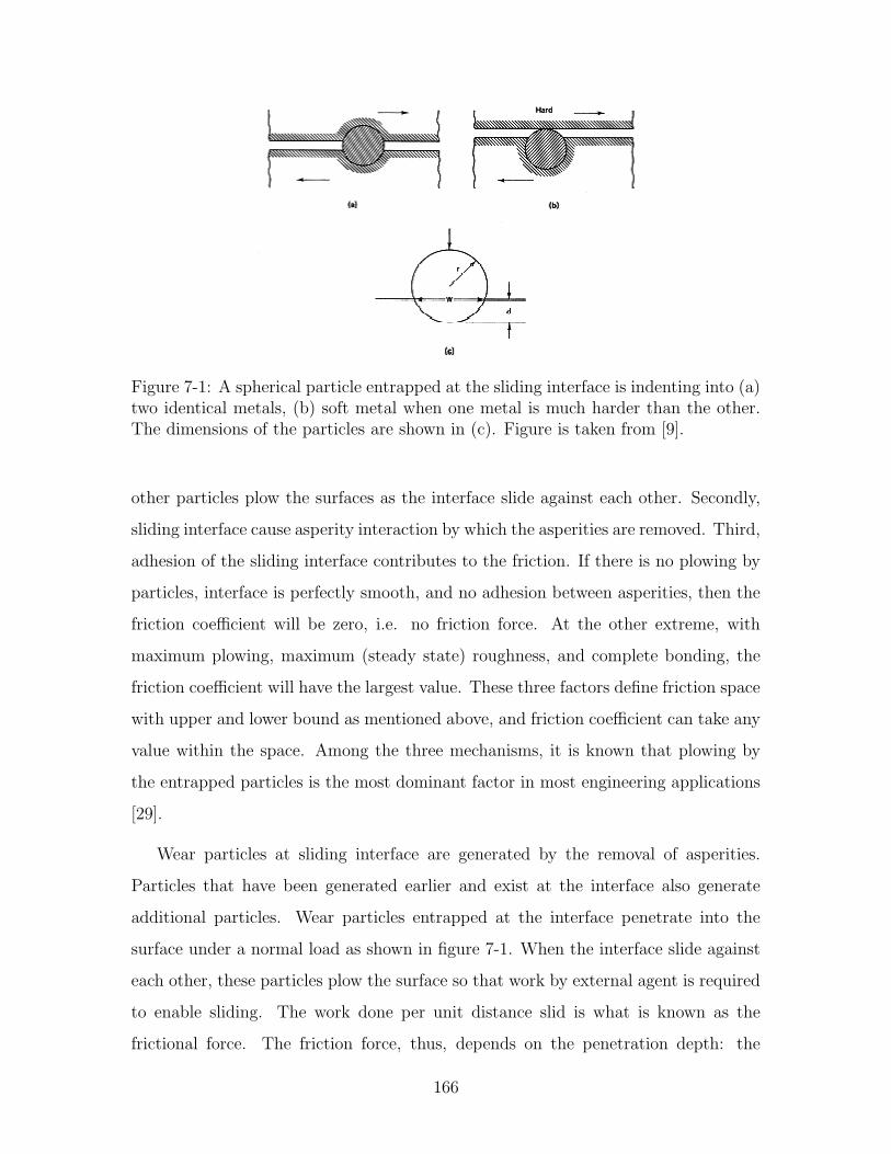
Figure 7-1: A spherical particle entrapped at the sliding interface is indenting into (a)two identical metals, (b) soft metal when one metal is much harder than the other.The dimensions of the particles are shown in (c). Figure is taken from [9].

other particles plow the surfaces as the interface slide against each other. Secondly,

sliding interface cause asperity interaction by which the asperities are removed. Third,

adhesion of the sliding interface contributes to the friction. If there is no plowing by

particles, interface is perfectly smooth, and no adhesion between asperities, then the

friction coefficient will be zero, i.e. no friction force. At the other extreme, with

maximum plowing, maximum (steady state) roughness, and complete bonding, the

friction coefficient will have the largest value. These three factors define friction space

with upper and lower bound as mentioned above, and friction coefficient can take any

value within the space. Among the three mechanisms, it is known that plowing by

the entrapped particles is the most dominant factor in most engineering applications

[29].

Wear particles at sliding interface are generated by the removal of asperities.

Particles that have been generated earlier and exist at the interface also generate

additional particles. Wear particles entrapped at the interface penetrate into the

surface under a normal load as shown in figure 7-1. When the interface slide against

each other, these particles plow the surface so that work by external agent is required

to enable sliding. The work done per unit distance slid is what is known as the

frictional force. The friction force, thus, depends on the penetration depth: the

166

Figure 7-2: Friction coefficient due to plowing component increases nonlinearly as afunction of the depth of penetration of the wear particle. Figure is taken from [9].

deeper particles penetrate into the surface, the more work is required to overcome

resistance. Indeed, friction coefficient increases nonlinearly as a function of the depth

of penetration of the wear particle (see figure 7-2).

7.2 Introducing Periodicity

As the interface slide continuously with wear particles entrapped between the sliding

surfaces, wear particles may agglomerate as shown in figure 7-3. Under the normal

load, a newly-generated particle undergoes plastic deformation and conforms to the

work-hardened asperity of the existing agglomerate, a process similar to cold com-

paction of metal powders or coining process [3]. Sooner or later, the growing agglom-

erate reaches a point where it cannot sustain the stress due to increased moments.

Then, the agglomerate breaks and new agglomerate begins to form. Thus, wear par-

ticle agglomeration has periodicity by itself. As many number of agglomerates follow

the periodicity, it reaches steady state overall.

As the particles agglomerate, the applied normal load is carried by a smaller

167

Figure 7-3: (a) An agglomerate wear debris is shown as a cylindrical shape, and(b)wear particles may agglomerate to form larger particles at the sliding interfacewhen there is sufficient pressure to deform the particles and cause bonding. Figure istaken from [3].

number of larger particles rather than by a large number of small particles. Assuming

the total wear volume is constant, the larger agglomerated particles penetrate deeper

into the surface than the smaller particles do. Recall that the friction coefficient

increases with the penetration depth of wear particle (figure 7-2). Therefore, friction

coefficient is expected to increase as agglomeration occurs, and the experimental

results reported in [3] show that is the case.

Natural periodicity of the particle agglomeration would result in the characteristic

maximum size of the agglomerates at steady state, which, in turn would lead to

steady state penetration depth. That will determine friction coefficient of the sliding

interface. Then, if we want to lower the friction coefficient, introducing periodicity

that is shorter – in terms of the size of agglomerates – than inherent periodicity.

7.2.1 Undulated Surface

Having understood the mechanism of surface friction, relevant design range is the size

of agglomerated wear particles. Then, the system range, actual size of wear particle,

drifts out of the design range as the interface slides continuously. Thus, it has to

be re-initialized to bring the system range back to initial system range. That is to

168

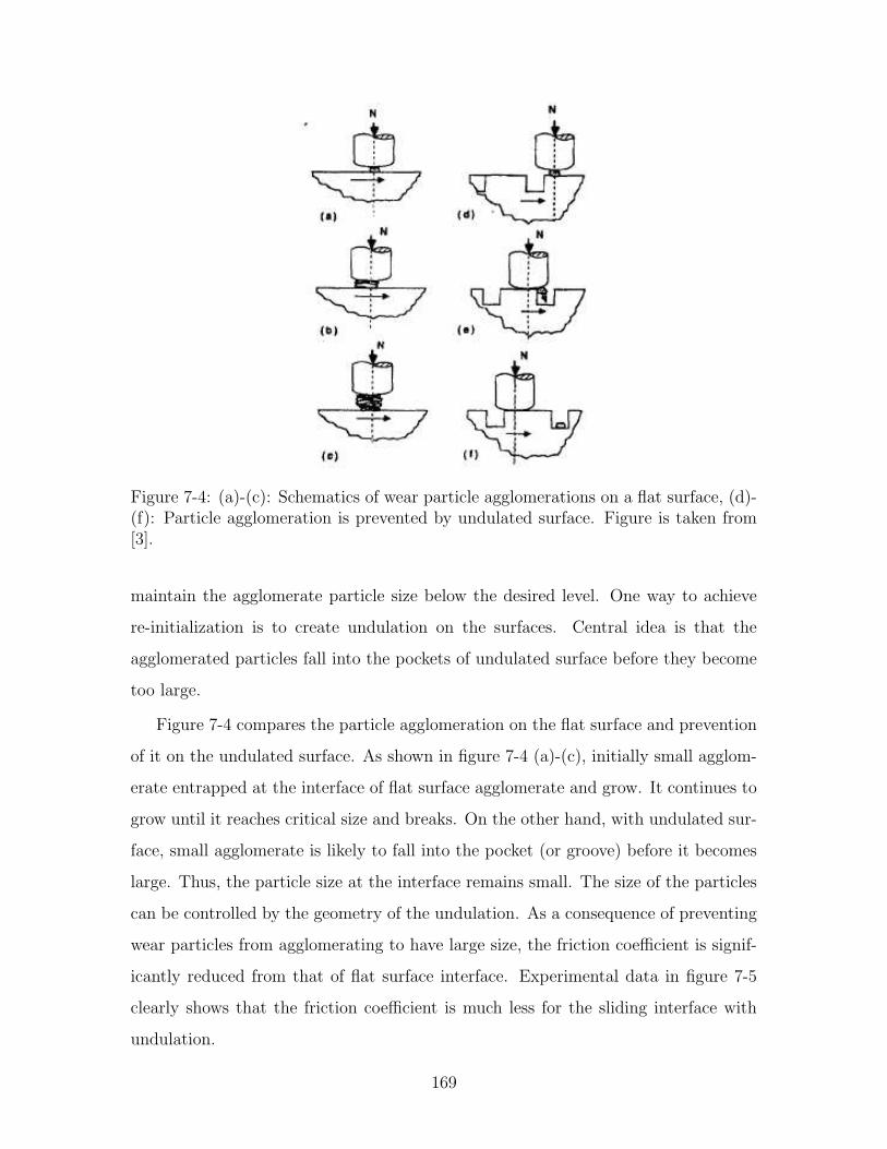
Figure 7-4: (a)-(c): Schematics of wear particle agglomerations on a flat surface, (d)-(f): Particle agglomeration is prevented by undulated surface. Figure is taken from[3].

maintain the agglomerate particle size below the desired level. One way to achieve

re-initialization is to create undulation on the surfaces. Central idea is that the

agglomerated particles fall into the pockets of undulated surface before they become

too large.

Figure 7-4 compares the particle agglomeration on the flat surface and prevention

of it on the undulated surface. As shown in figure 7-4 (a)-(c), initially small agglom-

erate entrapped at the interface of flat surface agglomerate and grow. It continues to

grow until it reaches critical size and breaks. On the other hand, with undulated sur-

face, small agglomerate is likely to fall into the pocket (or groove) before it becomes

large. Thus, the particle size at the interface remains small. The size of the particles

can be controlled by the geometry of the undulation. As a consequence of preventing

wear particles from agglomerating to have large size, the friction coefficient is signif-

icantly reduced from that of flat surface interface. Experimental data in figure 7-5

clearly shows that the friction coefficient is much less for the sliding interface with

undulation.

169

(a) (b)

Figure 7-5: Friction coefficient versus sliding distance in copper on (a)flat Zinc surfaceand (b)undulated zinc, sliding at 2.5N normal load and 0.01m/s sliding speed [3].

7.3 Summary

Design of low friction surface was discussed to illustrate how combinatorial complex-

ity can be transformed to periodic complexity. The transformation is achieved by

introducing geometric periodicity into the sliding interface.

Knowing that plowing by the entrapped particles is the dominant contributor to

the frictional force and that agglomeration of the wear particles increases the frictional

force, the relevant design range is the size of wear particles. As the interface continue

to slide against each other, the system range – actual size of agglomerate – moves

out of the design range. Thus, it has to be re-initialized. Undulated surface plays

a role of internal re-initialization and thereby maintains the particle size under the

desired value. By introducing periodicity that is short enough to prevent excessive

agglomeration, the interface achieves low friction coefficient.

170

Chapter 8

Conclusions

8.1 Complexity in Axiomatic Design

Although there exist many definitions for complexity concept, they do not properly

address issues that are important from engineering design standpoint, for example, a

relative aspect of design problem and causes of complexity. As a result, a concept of

complexity has a limited utility, or more often it is used as a metaphor to indicate the

difficulty associated in design/manufacturing/operation. The concept of complexity

defined in axiomatic design theory provides a useful framework to effectively discuss

causes of complexity and methods to reduce it.

Complexity in axiomatic design is defined as a measure of uncertainty in achiev-

ing the desired functional requirements. This definition of complexity incorporates

attributes such as difficulty, uncertainty, relativity, ignorance, and information. The

peculiarity of AD complexity concept can be well understood once those aspects of

the definition are recognized. There are four different sub-categories of AD com-

plexity: time-independent real complexity, time-independent imaginary complexity,

time-dependent periodic complexity, and time-dependent combinatorial complexity

(see figure 8-1). Time-dependent complexity consists of real and imaginary com-

plexity. Real complexity accounts for random nature of a system, and is equivalent

to information content since information content measures the uncertainty in the

same probability context. Imaginary complexity, on the other hand, accounts for the

171

ComplexityMeasure of uncertainty in achieving FR

Time-independentComplexity

Time-dependentComplexity

Realcomplexity

Imaginarycomplexity

Combinatorialcomplexity

Periodiccomplexity

Does uncertaintychange with time?

Figure 8-1: Four types of complexity are identified in axiomatic design. Dependingon the uncertainty’s time-dependence, it is divided into time-independent and time-dependent complexity. Time-independent complexity consists of real and imaginarycomplexity, and time-dependent complexity has combinatorial and periodic complex-ity.

uncertainty due to ignorance, particularly the ignorance of the structure of design

matrices. Time-dependent complexity is also divided into two different kinds: combi-

natorial complexity and periodic complexity. Uncertainty in a case of combinatorial

complexity increases continuously while periodic complexity ceases to increase at cer-

tain point and returns to initial level of uncertainty. A system has combinatorial

complexity when (1) its system range continues to drift away from design range and

(2) the functional requirements set FR(t) is unpredictable.

It is clear that the causes of complexity are embedded in its definition. Real

complexity is due to random variations associated in a design such as variations

in DPs and noise factors. The cause of imaginary complexity is the ignorance of

the structure of design matrices. For both combinatorial and periodic complexity,

the causes are time-varying system range and time-dependent FR. By identifying

what causes complexity, it is possible to develop a systematic approach to complexity

reduction.

172

8.2 Reduction of Complexity

Reducing real complexity is equivalent to reducing variation in functional require-

ments, which has been the topic of common engineering research and practices. They

include 1)eliminating source of variation, 2)desensitizing a system, and 3)compen-

sating for the variation. Based on technical and economic consideration, these three

approaches must be combined to yield optimal result. Imaginary complexity must be

eliminated by identifying the structure of design matrices and following one of the

correct sequences dictated by design matrices.

By definition of time-dependent complexity, uncertainty of a system with combi-

natorial complexity increases indefinitely while in case of a system with periodic com-

plexity, it ceases to increase at certain point and returns to initial level of uncertainty.

In order to prevent uncertainty from ever-increasing and to maintain complexity un-

der a manageable limit, combinatorial complexity should be avoided. Transforming

combinatorial complexity into periodic complexity is referred to as re-initialization.

When a system experiences combinatorial complexity due to a time-varying sys-

tem range issue, functional requirements are becoming more difficult to achieve as

time elapses. Thus, periodically recovering the initial system range is important.

Periodically bringing back the system range is equivalent to transforming the combi-

natorial complexity to periodic complexity. The act of achieving this transformation

is one type of re-initialization, in a sense that the system is re-initialized to its ini-

tial state in terms of the associated uncertainty. Re-initialization of time-varying

system range can be done externally or internally. While preventive maintenance

and statistical process control are common examples of external re-initialization, the

low friction surface design example illustrate how the system range can be self-re-

initialized internally by design. A clever design as in knob example in section 3.1.1

can help minimizing the cost of external re-initialization by delaying the deterioration

of system range.

Whether a system has combinatorial or periodic complexity can also depend on

the type of periodicity present in time-dependent functional requirements set FR.

173

It was shown by probability of success and predictability of FR that periodic and

semi-periodic FR result in periodic complexity whereas aperiodic FR leads to com-

binatorial complexity. Functional periodicity is achieved by establishing appropriate

initial states repeatedly in a system, and that is the second type of re-initialization.

Two examples are drawn from different fields to support the argument on the role

of functional periodicity in achieving successful system functionality. First example is

a scheduling of part-transport in an integrated system with process time variation. In

the example, it was shown that break-down of functional periodicity in one of the sub-

systems results in sub-optimal throughput performance of the integrated system. In

order to ensure the productivity and reliability of such system, functional periodicity

must be maintained by re-initializing the subsystems on a periodic functional interval,

meaning each and every functional requirement is completed in every period. This

is equivalent to preventing a system from developing time-dependent combinatorial

complexity and thereby increases predictability of system performance and produc-

tivity. Second example is drawn from biological world where periodicity is commonly

observed at various scales. Among the abundant examples of biological systems with

periodicity, the eukaryotic cell cycle is examined with particular emphasis on its func-

tional periodicity. To maintain periodicity is an important functional requirement in

the cell division cycle rather than periodicity being a result or reflection of something

else. By achieving periodicity, cells are able to manage the level of complexity for

their survival. In addition, coordinating centrosome cycle and chromosome cycle is

analogous to integrating multiple subsystems to form a manufacturing system that

was discussed in chapter 5. By recognizing the analogy, it is possible to examine the

problem with a new perspective. This type of new ways of looking at the problem

can contribute to the study of biological systems.

These examples illustrate a critical role of functional periodicity in achieving de-

sired functional requirements. In many cases, loss of periodicity or lack thereof results

in chaotic behavior of a system and even leads to failure of a system. Introducing

functional periodicity by re-initialization ensures that a system does not develop a

combinatorial complexity.

174

8.3 Suggestions for Future Research

This thesis has discussed axiomatic design’s complexity concept to make progress to-

ward the following goals: 1) to avoid the vague usage of the term in the engineering

design discipline, 2) to acquire deeper insight into possible cause of complexity in

engineering design, and 3) to develop a systematic approach to complexity reduction.

While this thesis effectively addresses all three goals, further research will only im-

prove our understanding and broaden the applicability of the concept. Development

of systematic approach to complexity reduction must be on-going research topic.

In particular, developing quantifiable metric for time-dependent complexity is

one of the challenging research topics along the line. Indeed, with a comprehensive

complexity metric, the information axiom may be restated in terms of complexity.

Another interesting topic is to investigate more on creating periodicity as opposed to

maintaining inherent periodicity. For example, job shop scheduling requires defining

or creating periodicity in the system which is not naturally present in it. Finally,

it will broaden the scope of application of periodicity concept if periodicity in many

different domains other than temporal domain is investigated.

175

Bibliography

[1] Grassberger P. Problems in quantifying self-organized complexity. Helvetica

Physica Acta, 62:498–511, 1989.

[2] Suh N.P. Axiomatic Design: Advances and Applications. Oxford University

Press, New York, NY, 2001.

[3] Oktay S.T. and Suh N.P. Wear debris formation and agglomeration. Journal of

Tribology, 114:379–393, April 1992.

[4] Alberts B., Johnson A., Lewis J., Raff M., Roberts K., and Walter P. Molecular

Biology of the Cell, section 17, page 984. Garland Science, New York, NY, forth

edition, 2002.



edition, 2002.


Biology of the Cell. Garland Science, New York, NY, forth edition, 2002.


Biology of the Cell, section 18, pages 1034–1035. Garland Science, New York,

NY, forth edition, 2002.

[8] Nigg E.A. Centrosome aberrations: Cause or consequence of cancer progression.

Nature Reviews: Cancer, 2:1–11, November 2002.

177

[9] Suh N.P. and Sin S.-C. The genisis of friction. Wear, 69:91–114, 1981.



edition, 2002.

[11] Edmonds B. Syntactic measures of complexity. PhD dissertation, University of

Manchester, Department of Philosophy, 1999.

[12] Gell man M. and Lloyd S. Information measures, effective complexity, and total

information. Complexity, 2:44–52, 1996.

[13] Baranger M. Chaos, complexity, and entropy. http://necsi.org/projects/. Pub-

lished on WWW; access in 2001.

[14] Chakrabarti C.G. and De K. Boltzmann-gibbs entropy: Axiomatic characteriza-

tion and application. International Journal of Math. and Math. Science, 23:243–

251, 2000.

[15] Shannon C.E. A mathematical theory of communication. The Bell System Tech-

incal Journal, 27:379–423, 623–656, 1948.

[16] Cover T.M. and Thomas J.A. Elements of Information Theory. Wiley Searies

in Telecommunications. A Wiley-Interscience Publication, 1991.

[17] Sipser M. Introduction to the Theory of Computation. PWS Publishing Company,

Boston, MA, 1997.

[18] Bennett C.H. Logical depth and physical complexity. In R. Herken, editor,

The Universal Turing Machine, A Half-Century Survey, pages 227–257. Oxford

University Press, Oxford, UK, 1988.

[19] Mikulecky D.C. Definition of complexity. http://views.vce.edu/ mikuleck/. Pub-

lished on WWW; accessed in 2001.

[20] Suh N.P. A theory of compelxity, periodicity, and design axioms. Research in

Engineering Design, 11:116–131, 1999.

178

[21] Carlson J.M. and Doyle J. Complexity and robustness. In Proceedings of the

National Academy of Sciences, number 99, pages 2538–2545, February 2002.

[22] Klir G.J. and Folger T.A. Fuzzy Sets, Uncertainty, and Information. Prentice

Hall, 1988.

[23] Frey D.D., Jabangir E., and Engelhardt F. Computing the information content

of decoupled designs. In Proceedings of the First International Conference on

Axiomatic Design, pages 151–161, Cambridge, MA, June 2000.

[24] Suh N.P. and Lee T. Reduction of complexity in manfuacturing systems through

the creation of time-dependent periodic complexity from time-dependent combi-

natorial complexity. Keynote Paper at the 35th CIRP-International Seminar on

Manufacturing Systems, Seoul, Korea, May 2002.

[25] Lee T. The system architecture concept in axiomatic design theory: Hypotheses

generation and case-study validation. Master’s thesis, MIT, Dept. of Mechanical

Engineering, June 1999.

[26] Melvin J.W. Axiomatic System Design: Chemical Mechanical Polishing Machine

Case Study. PhD dissertation, MIT, Dept. of Mechanical Engineering, February

2003.

[27] Suh N.P. Design and operation of large systems. Journal of Manufacturing

Systems, 14(3):203–213, 1995.

[28] Suh N.P. Tribophysics. Prentice-Hall, Englewood Cliffs, NJ, 1986.

[29] Suh N.P. Design of engineered tribological systems. Talk at the South African

Conference on Tribology at Pretoria, South Africa, 2001.

[30] Perkinson T.L., Gyurcsik R.S., and McLary P.K. Single-wafer cluster tool per-

formance: An analysis of the effects of redundant chambers and revisitation

sequences on throughput. IEEE Transactions on Semiconductor Manufacturing,

9:384–400, August 1996.

179

[31] Jevtic D. Method and apparatus for automatically generating schedules for

wafer processing within a multichamber semiconductor wafer processing tool.

US Patent & Trademark Office, 2001.

[32] Oh H.L. and Lee T. A synchronous algorithm to reduce complexity in wafer

flow. In Proceedings of the First International Conference on Axiomatic Design,

pages 87–92, Cambridge, MA, June 2000.

[33] Oh H.L. Reducing complexity of wafer flow to improve quality and throughput

in a single-wafer cluster tool. In IEEE/CPMT International Electronics Manu-

facturing Technology Symposium, pages 378–388, 1999.

[34] Perkinson T.L., McLary P.K., Gyurcsik R.S., and Cavin R.K. Single-wafer clus-

ter tool performance: An analysis of throughput. IEEE Transactions on Semi-

conductor Manufacturing, 7:369–373, August 1994.

[35] Wood S.C. Simple performance models for integrated processing tools. IEEE

Transactions on Semiconductor Manufacturing, 9(3), 1996.

[36] Lopez M.J. and Wood S.C. Performance models of systems of multiple cluster

tools. In 1996 IEEE/CPMT International Electronics Manufacturing Technology

Symposium, pages 57–65, 1996.

[37] Rostami S., Hamidzadeh B., and Camporese D. An optimal scheduling technique

for dual-arm robots in cluster tools with residency constraints. In The 39th IEEE

Conference on Decision and Control, pages 3459–3464, December 2000.

[38] Song W., Zabinsky Z.B., and Storch R.L. An algorithm for scheduling a chemical

processing tank line. Production Planning and Control, 4:323–332, 1993.

[39] Levner E., Kats V., and Sriskandarajah C. A geometric algorithm for finding

two-unit cyclic schedules in a no-wait robotic flowshop. In Proceedings of the

International Workshop on Intelligent Scheduling of Robots and Flexible Manu-

facturing Systems, pages 101–112, Holon, Israel.

180

[40] Kats V., Levner E., and Meyzin L. Multiple-part cyclic hoist scheduling using

a sieve method. IEEE Transactions on Robotics and Automation, 15:704–713,

1999.

[41] Che A., Chu C., and Chu F. Multicyclic hoist scheduling with constant processing

times. IEEE Transactions on Robotics and Automation, 18(1), February 2002.

[42] Lee T. and Suh N.P. Reduction of complexity of manufacturing systems through

the creation of time-dependent periodic complexity from time-dependent combi-

natorial complexity. To be published, 2002.

[43] Compton D.A. Spindle assembly in animal cells. Annual Review of Biochemistry,

69:95–114, 2000.

[44] Megraw T.L., Kao L.R., and Kaufman T.C. Zygotic development without func-

tional mitotic centrosomes. Current Biology, 11:116–120, 2001.

[45] Kramer A., Neben K., and Ho A.D. Centrosome replication, genomic instability

and cancer. Leukemia, 16:767–775, 2002.

[46] Bobinnec Y., Khodjakov A., Mir L.M., Rieder C.L., Edde B., and Bornens M.

Centriole disassembly in vivo and its effect on centrosome structure and function

in vertebrate cells. Journal of Cell Biology, 143:1575–1589, 1998.

[47] Stearns T. Centrosome duplication: A centriolar pas de deux. Cell, 105:417–420,

2001.

[48] Lacey K.R., Jackson P.K., and Stearns T. Cyclin-dependent kinase control of

centrosome duplication. In Proceedins of National Academy of Science, num-

ber 96, pages 2817–2822, 1999.

[49] Matsumoto Y., Hayashi K., and Nishida E. Cyclin-dependent kinase 2(cdk2)

is required for centrosome duplication in mammalian cells. Current Biology,

9:429–432, 1999.

181

[50] Meraldi P., Lukas J., Fry A.M., Bartek J., and Nigg E.A. Centrosome duplication

in mammalian somatic cells requires e2f andcdk2-cyclin a. Nature Cell Biology,

1:88–93, 1999.

[51] Okuda M., Horn H.F., Tarapore P., Tokuyama Y., Smulian A.G., Chan P-K.,

Knudsen E.S., Hofmann I.A., Snyder J.D., Bove K.E., and Fukasawa K. Nu-

cleophosmin/b23 is a target of cdk2/cyclin e in centrosome duplication. Cell,

103:127–140, 2000.

[52] Matsumoto Y. and Maller J.L. Calcium, calmodulin, and camkii requirement for

initiation of centrosome duplication in xenopus egg extracts. Science, 295:499–

502, January 2002.

[53] O’Connell K.F., Caron C., Kopish K., Hurd D.D., Kemphues K.J., Li Y., and

White J.G. The c. elegans zyg-1 gene encodes a regulator of centrosome duplica-

tio nwith distinct maternal and paternal roles in the embryo. Cell, 105:547–558,

2001.

[54] Sluder G. and Hinchcliffe E.H. The coordination of cetnrosome reprodevents

during the cell cycle. Current Topics in Developmental Biology, 49:267–289,

2000.

182

Complexity Theory in Axiomatic Designweb.mit.edu/pccs/pub/2003/tlee-complexity.pdf · Complexity...

Documents

Transcript of Complexity Theory in Axiomatic Designweb.mit.edu/pccs/pub/2003/tlee-complexity.pdf · Complexity...