Complexity: Revealed Preference and Equilibriumfede/slides/compcom.pdf · Complexity: Revealed...
87
Complexity: Revealed Preference and Equilibrium Federico Echenique California Institute of Technology MSR – March 29, 2013
Transcript of Complexity: Revealed Preference and Equilibriumfede/slides/compcom.pdf · Complexity: Revealed...

Complexity: Revealed Preference and Equilibrium
Federico Echenique
California Institute of Technology
MSR – March 29, 2013

Three papers:
I A Revealed Preference Approach to ComputationalComplexity in Economics, by Echenique, Golovin & Wierman.
I Finding a Walrasian equilibrium is easy for a fixed number ofagents, by Echenique & Wierman
I The Empirical Implications of Rank in Bimatrix Games, byBarman, Bhaskar, Echenique, & Wierman.

CS and Economics
Recent interest from the theoretical CS literature in economicmodels. Important new results on our basic models of agents,markets and strategic interactions.
Many basic results are negative:
I Utility functions are hard to maximize;
I Nash equilibrium is hard to find;
I Walrasian equilibrium is hard to find.

CS critique of positive economics:
Economics is flawed because it assumes agents/society solve hardproblems.
“As rational as consumers can possibly be, it is unlikelythat they can solve in their minds problems that proveintractable for computer scientists equipped with thelatest technology.”
– Gilboa, Schmeidler & Postlewaite
“If an equilibrium is not efficiently computable, much ofits credibility as a prediction of the behavior of rationalagents is lost”
– Christos Papadimitriou
“If your laptop cannot find it, neither can the market”
– Kamal Jain

Theory of the consumer.
“As rational as consumers can possibly be, it is unlikelythat they can solve in their minds problems that proveintractable for computer scientists equipped with thelatest technology.”
– Gilboa, Schmeidler & Postlewaite

Methodological positivism.
CS (Bded. rationality) critique misunderstands the role of modelsin positive economics.
Model is a way of thinking about reality, i.e. about data.
Economic theory only states that reality behaves as if the theory istrue.

Question: What is the empirical content of the hypothesis thatconsumers are boundedly rational (i.e. that they can’t solve hardproblems).
Answer: None.

Question: What is the empirical content of the hypothesis thatconsumers are boundedly rational (i.e. that they can’t solve hardproblems).
Answer: None.
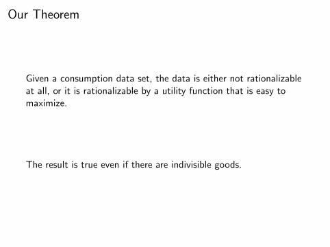
Our Theorem
Given a consumption data set, the data is either not rationalizableat all, or it is rationalizable by a utility function that is easy tomaximize.
The result is true even if there are indivisible goods.
Digression: complexity for economists.

Complexity for dummies.
Economists’ reaction to complexity:
I May make sense for computers, notfor people/economies.
I Worst case analysis.

Complexity for dumm. . . economists!
A decision problem is a problem with a yes/no answer.Let A be a class of dec. problems.
A dec. problem α is A-hard if there is an algorithm that easilytransforms any instance of a problem in A into an instance of α,and preserves the answer.
So if you have an algorithm to solve α, you have an algorithm tosolve any problem in A. Or, α is as hard as anything in A.
Ex: NP-hard problems.
Primitives
n = number of goodsX ⊆ Rn
+ is consumption spacewe assume X ⊆ Zn
+

Data sets
A consumption data set D is a collection (xk , pk), k = 1, . . .K ,with xk ∈ X and pk ∈ Rn
++.
I xk is the consumption bundle
I purchased at prices pk .

Rationalization
A utility u : X → R rationalizes the data if,for all k and y ∈ X ,
(pk · y ≤ pk · xk and y 6= xk)⇒ u(xk) > u(y).
Are all data sets rationalizable?

x1
x2
p1
p2
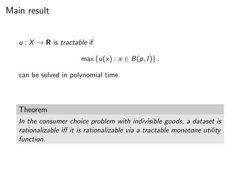
Main result
u : X → R is tractable if
max u(x) : x ∈ B(p, I ) .
can be solved in polynomial time.
Theorem
In the consumer choice problem with indivisible goods, a dataset isrationalizable iff it is rationalizable via a tractable monotone utilityfunction.

Two approaches in revealed pref. theory
I Construct a utility
I Extend demand.

Constructing a utility does not work.
Theorem (Chambers & Echenique)
In the consumer choice problem with indivisible goods, thefollowing statements are equivalent:
I The dataset is rationalizable.
I The dataset is rationalizable by a supermodular utilityfunction.
I The dataset is rationalizable by a submodular utility function.
Max. of a super/sub-modular utility subject to a budget constraintis hard.

Revealed preference
x is revealed preferred to y ifthere is k s.t. x = xk and pky ≤ pkxk
Indicate revealed preference with →.

x1x2
x3

x1 x2
x3

x1x2
x3


Algorithm:
I Construct a (strict) preference on data points s.t. extends the rev. pref.
I Given p and m choose a maximal point in B(p,m) by:
1. Choose best data point z in B(p,m) for .2. Project z into the budget line lexicographically.
The algorithm defines a demand function d(p,m).We show that it is a rational demand: it satisfies SARP.

A violation of WARP
x1
x2
p1
p2
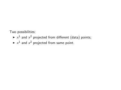
Two possibilities:
I x1 and x2 projected from different (data) points;
I x1 and x2 projected from same point.

x1
x2

x1
x2

x1
x2

Running time of algorithm depends on size of the data set. Thisturns out to be unavoidable.
Proposition
Any algorithm that takes as input a data set with n data points, aprice vector p, and an income I and outputs d(p, I ) for a d whichrationalizes the data set requires, in the worst case, Ω(n) runningtime on a RAM with word size Θ(log n), even when there are onlytwo goods.
Proposition
Any demand function d that rationalizes a data set with n datapoints requires Ω(n log n) bits of space to represent, in the worstcase, even when there are only two goods.

Now: general equilibrium theory.
“If your laptop cannot find it, neither can the market”
– Kamal Jain

CS and Economics
For the model of general equilibrium, main CS result is:
Walrasian equilibrium is hard to find.
Hard, even if:
I Utilities are separable over goods and piecewise linear(concave).
I Utilities are Leontief

Our results
Consider exchange economies with std. assumptions on preferences(smooth concave utilities); n agents and l goods.
When n is fixed, it’s easy to find a WE.
Exploits the Negishi approach to prove existence of WE.

Why study n fixed?
Macro & finance models → many goods, few agents.
I Models w/representative agent.
I Models with n agents and infinitely many goods.
Literally fixed n.

Why study n fixed?
The history of all hitherto existing society is the historyof class struggles.
– Karl Marx
Many agents but limited heterogeneity: economic “class.”
If preferences are homothetic, and all agents belong to one of afixed number of endowment classes (e.g. farmers, workers andcapitalists), then WE is easy.

Why study n fixed?
Popular model of a large economy: replica of a given economy.
Many classical results on large economies, such as coreconvergence, hold for replica economies.
Our result implies that WE is easy for (large) replica economies.

Digression: complexity for economists.

Complexity for dummies
Economists’ reaction to complexity:
I May make sense for computers, notfor people/economies.
I Worst case analysis.

Complexity for dumm. . . economists!
A decision problem is a problem with a yes/no answer.Let A be a class of dec. problems.
A dec. problem α is A-hard if there is an algorithm that easilytransform any instance of a problem in A into an instance of α,and preserves the answer.
So if you have an algorithm to solve α, you have an algorithm tosolve any problem in A. Or, α is as hard as anything in A.
Ex: NP-hard problems.

Complexity for dumm. . . economists!
Decision problems are not appropriate for equilibria, becauseexistence is guaranteed.
Class of problems based on computing a (total) function: given aninput x , compute f (x).
A problem is PPAD-hard if it is as hard as END OF THE LINE.Finding Walrasian eq. with Leontief utilities is PPAD-hard.


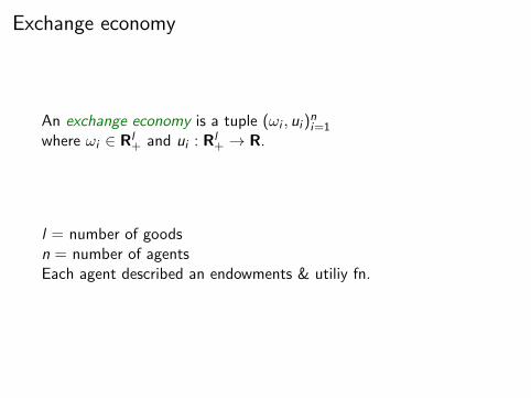
Exchange economy
An exchange economy is a tuple (ωi , ui )ni=1
where ωi ∈ Rl+ and ui : Rl
+ → R.
l = number of goodsn = number of agentsEach agent described an endowments & utiliy fn.

Exchange economy
An allocation in (ωi , ui )ni=1 is
x ∈ Rnl+ s.t.
∑ni=1 xi =
∑ni=1 ωi .
A Walrasian equilibrium in (ωi , ui )ni=1 is (p, x) s.t.
1. (p a price vector),
2. (supply equals demand)
3. (agents maximize utility when consuming xi )

Exchange economy
An allocation in (ωi , ui )ni=1 is
x ∈ Rnl+ s.t.
∑ni=1 xi =
∑ni=1 ωi .
A Walrasian equilibrium in (ωi , ui )ni=1 is (p, x) s.t.
1. (p a price vector),
2. (supply equals demand)
3. (agents maximize utility when consuming xi )

Exchange economy
An allocation in (ωi , ui )ni=1 is
x ∈ Rnl+ s.t.
∑ni=1 xi =
∑ni=1 ωi .
A Walrasian equilibrium in (ωi , ui )ni=1 is (p, x) s.t.
1. (p a price vector), p ∈ Rl++
2. (supply equals demand) x = (xi )ni=1 ∈ Rnl
+ is an allocation,
3. (agents maximize utility when consuming xi ) and for all ip · ωi = p · xi and
ui (y) > ui (xi )⇒ p · y > p · xi

Approximate equilibrium
A Walrasian ε-equilibrium is (p, x) s.t.
1. p ∈ Rl+,
2. x is an allocation,
3. and for all i
ui (y) > ui (xi )⇒ p · y > p · xi
and |p · ωi − p · xi | < ε.

E a family of exchange economies.
Each (ui , ωi )ni=1 ∈ E has n agents (different numb. goods);
assume:
1. (all goods exist)∑n
i=1 ωi ∈ Rl++;
2. (regular utilities) ui is C 1, concave, and strictly monotonic;
3. (boundary condition) If x ∈ Rl+ \ Rl
++ and y ∈ Rl++, then
u(x) < u(y);
4. (normalization) ∀x ∈ Rnl+ s.t.
∑ni=1 ωi =
∑ni=1 xi ,
ui (xi ) ∈ [0, 1].

Theorem
Let ε > 0. There is an algorithm that, for any economy in E , findsa Walrasian ε-equilibrium in time polynomial in l .
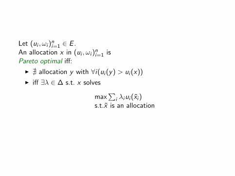
Let (ui , ωi )ni=1 ∈ E .
An allocation x in (ui , ωi )ni=1 is
Pareto optimal iff:
I @ allocation y with ∀i(ui (y) > ui (x))
I iff ∃λ ∈ ∆ s.t. x solves
max∑
i λiui (xi )s.t.x is an allocation

A Walrasian equilibrium with transfers is a triple (p, x ,T ), where:
I p ∈ Rl+ (a vector of prices);
I T ∈ Rn and∑n
i=1 Ti = 0 (a vector of transfers);
I x is an allocation (supply equals demand);
I ∀iui (y) > ui (xi )⇒ p · y > p · ωi + Ti
and p · xi = p · ωi + Ti (agents are maximizing utility).
Note: a WE is a WET with zero transfers; an approximate WE is aWET with small transfers.

Second Welfare Theorem
Theorem
Let (ui , ωi )ni=1 ∈ E and x be an interior Pareto optimal allocation.
Then ∃ p and T s.t. (x , p,T ) is Walrasian eq. with transfers.

Negishi’s approach
λ ∈ ∆ // x(λ) ∈ argmax∑
i λiui // (x(λ), p(λ),T (λ))
_
λ′ ∈ ∆
Existence follows by Kakutani’s FPT.Note the fixed-point argument is in the n-dimensional simplex.

Negishi’s approach
We:
I Kakutani is non-constructive.Instead we use Sperner’s lemma.
I Find a zero of T (λ).
I Approximation must be independent of l .
λ ∈ ∆ // x(λ) ∈ argmax∑
i λiui // (x(λ), p(λ),T (λ))

SWT for undergrads
max∑n
i=1 λiui (xi )
s.t.
∑ni=1 xi ≤
∑ni=1 ωi
xi ≥ 0.
p(λ) = λhDui (xh(λ)).
Ti (λ) = p(λ) · (xi (λ)− ωi ).
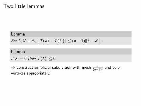
Two little lemmas
Lemma
For λ, λ′ ∈ ∆, ‖T (λ)− T (λ′)‖ ≤ (n − 1)‖λ− λ′‖.
Lemma
If λi = 0 then T (λ)i ≤ 0.
⇒ construct simplicial subdivision with mesh ε(n−1)2 and color
vertexes appropriately.


Sperner’s lemma to get ‖T‖ < ε
I simplicial subdivision with mesh ε(n−1)2
I for λ, λ′ in same subsimplex, T (λ) close to T (λ′) (Lipschitzlemma)
I color subdivision: vertex λ has color i if Ti (λ) > 0 (chooselargest Ti (λ) if more than one).
I Boundary lemma ⇒ proper labeling of subsimplex
I polychromatic subsimplex gives T (λ) close to each other, foreach i one λ with Ti (λ) > 0.
I Since∑
i Ti (λ) = 0 must have ‖T (λ)‖ < ε.
Other notions of approximate equilibria.

Other notions of approximation
An ε-approximate equilibrium in an exchange economy (ui , ωi )ni=1
is a pair (p, x) where p ∈ Rl+, x is an allocation, and for all i
p · y ≤ p · ωi ⇒ ui (y) ≤ ui (xi ) + ε,
and |p · ωi − p · xi | < ε.
A defn. like the one used in CS.
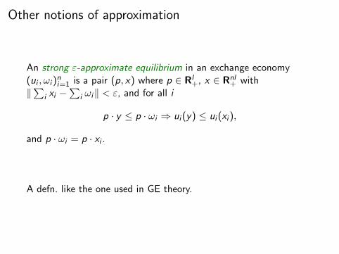
Other notions of approximation
An strong ε-approximate equilibrium in an exchange economy(ui , ωi )
ni=1 is a pair (p, x) where p ∈ Rl
+, x ∈ Rnl+ with
‖∑i xi −∑
i ωi‖ < ε, and for all i
p · y ≤ p · ωi ⇒ ui (y) ≤ ui (xi ),
and p · ωi = p · xi .
A defn. like the one used in GE theory.

Other notions of approximation
Suppose that there is Θ > 0 and π > 0 such that, for all(ui , ωi )
ni=1 in E ,
supp∈∆
p ·n∑
i=1
ωi ≤ Θ,
and if x is an allocation in (ui , ωi )ni=1, then Dsui (xi ) > π.

Other notions of approximation
Theorem
Let ε > 0. There is an algorithm that, for any economy in E , findsan ε-approximate equilibrium, and a strong ε-approximateequilibrium, in time polynomial in l .

Now: game theory.
The Empirical Implications of Rank in Bimatrix Games, byBarman, Bhaskar, Echenique, & Wierman.

Nash equilibrium
A two-player game in normal form is given by a pair of matrices(A,B) of size n × n,A Nash equilibrium is a pair (i , j) ∈ [n]× [n] s.t. ∀ i ′ ∈ [n] andj ′ ∈ [n],
Aij ≥ Ai ′j and Bij ≥ Bij ′ .
If inequalities are strict, then (i , j) is a strict Nash equilibrium.

Rank
Our focus is on games with low rank.The rank of a game (A,B) is the rank of the matrix C := A + B.For a zero-sum game, C = 0.

Data
A subgame is denoted by (I , J) where I , J ⊆ [n]A data set is a set of triples ((i , j), I , J), where (I , J) is a subgame,and i ∈ I and j ∈ J.
Revealed Preference
A data set T is rationalizable if there exist a game (A,B) s.t. (i , j)is a strict Nash eq. in the subgame (I , J), ∀((i , j), I , J) ∈ T .
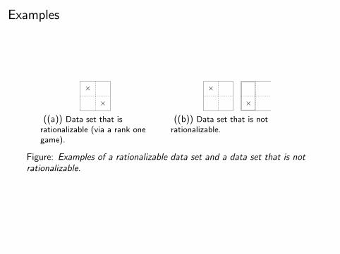
Examples
××
((a)) Data set that isrationalizable (via a rank onegame).
××
((b)) Data set that is notrationalizable.
Figure: Examples of a rationalizable data set and a data set that is notrationalizable.

Crossing number
Two subgames (I , J) and (I ′, J ′) cross if (I × J) ∩ (I ′ × J ′) 6= ∅,but (I × J) 6⊆ (I ′ × J ′) and (I ′ × J ′) 6⊆ (I × J).
The crossing number of T is
min |i : (i , j) ∈ O| , |j : (i , j) ∈ O| .

Theorem
For all n, there exists a rationalizable data set T over an n × nstrategy space such that the rank of any bimatrix game thatrationalizes T is Ω(
√n).

Theorem
Any rationalizable data set T that satisfies the uniqueness propertycan be rationalized by a bimatrix game of rank at most thecrossing number of T .

Despite all the computationsYou could just dance to that rock ’n’ roll stationAnd baby it was allright
– Lou Reed