Complexity and stochastic evolution of dyadic networks

Computers & Operations Research 33 (2006) 312–327

www.elsevier.com/locate/cor

Complexity and stochastic evolution of dyadic networks

Richard Barona, Jacques Durieua, Hans Hallerb,∗, Philippe Solala

aCREUSET, University of Saint-Etienne, 42023 Saint-Etienne, FrancebDepartment of Economics, Virginia Polytechnic Institute and State University, Blacksburg, VA 24061-0316, USA

Available online 23 July 2004

Abstract

A strategic model of network formation is developed which permits unreliable links and organizational costs.Finding a connected Nash network which guarantees a given payoff to each player proves to be anNP-hard problem.For the associated evolutionary game with asynchronous updating and logit updating rules, the stochastically stablenetworks are characterized.The organization of agents into networks has an important role in the communication of information within a

spatial structure. One goal is to understand how such networks form and evolve over time. Our agents are endowedwith some information which can be accessed by other agents forming links with them. Link formation is costlyand communication not fully reliable. We model the process of network formation as a non-cooperative game,and we then focus on Nash networks. But, showing existence of a Nash network with particular properties andcomputing one are two different tasks. The aim of this paper is to show that computing a connected Nash networkis a computationally demanding optimization problem. The question then arises what outcomes might be chosenby agents who would like to form a connected Nash network but fail to achieve their goal because of computationallimitations.We propose a stochastic evolutionary model. By solving a companion global optimization problem, thismodel selects a subset of Nash networks referred to as the set of stochastically stable networks.� 2004 Elsevier Ltd. All rights reserved.

Keywords:Game theory; Network formation; NP-hardness; Potential games; Stochastic stability

1. Introduction

Communication and information networks are of interest in artificial intelligence, computer science,economics, electrical engineering, neuroscience, and sociology, among others. The emphasis has been

∗ Corresponding author. Tel.: +1-540-231-7591; fax: +1-540-231-5097.E-mail address:[email protected](H. Haller).

0305-0548/$ - see front matter� 2004 Elsevier Ltd. All rights reserved.doi:10.1016/j.cor.2004.06.006

http://www.elsevier.com/locate/cor

mailto:[email protected]

R. Baron et al. / Computers & Operations Research 33 (2006) 312 – 327 313

on the functions and properties of networks and to a lesser degree on the formation and reconfigurationof networks. Here we develop a non-cooperative model of network formation with unreliable links andorganizational costs. In the dynamic version, we study the stochastic evolution of network architecturesand characterize the set of stochastically stable networks.The basic premise of our model is that deliberate individual or group decisions lead to the formation

or transformation of networks, like in the recent game-theoretic literature. The oldest strand of thatliterature originates with Myerson[1] and belongs to the domain of cooperative game theory. Jacksonand Wolinsky[2] introduced the concept of pairwise stability (known from the matching literature) asan equilibrium concept in models of network formation and gave rise to a second strand of literaturewhich can be characterized as semi-cooperative. A third game-theoretic approach to network formationhas been pioneered by Bala and Goyal[3] and is purely non-cooperative in nature. We follow the lattertradition and consider a network as the outcome of a non-cooperative or strategic game. The canonicalsolution concept for the static game is Nash equilibrium.The central assumption underlying Nash equilibrium and standard game theory is omniscience and full

rationality of players.As a practical matter, however, finding a Nash equilibrium of a gamemay consumetime and, perhaps, take too long. It turns out that finding a connected Nash network which guaranteesa given payoff to each player is an NP-hard problem with respect to the number of players, despite thesimplicity of our network formation game. Therefore, the question arises what outcomesmight be chosenby players who would like to form a Nash network, but fail to achieve their goal in reasonable amountof time because of computational limitations. Theories of bounded rationality aim to model how playerswould proceed in such a situation. Our own approach has two roots, one in evolutionary game theory andone in computer science.On the one hand, recent trends in game theory study adaptive learning models, in which players

or agents have limited cognitive and computational capacities and act according to boundedly rationalbehavior rules. Decisions taken on the basis of myopic best responses, reinforcement rules, imitation, orother short-sighted rules, coalesce in the long-run into limit sets or conventions. In the dynamic versionof our model, we assume asynchronous updating and that players choose myopic best responses whenthey have the opportunity to update. In addition, players make mistakes according to a logit rule. Thelatter implies that more severe mistakes are less likely.On the other hand, the use of heuristic methods in computer science is now standard for the approxima-

tion of solutions of computationally demanding global optimization problems. Most of them are based onperturbed iterative processes which are well suited to study adaptive evolution of a population of decisionmaking units. The objective of these methods is to globally optimize a function of a discrete finite systemcharacterized by a large number of solutions. Our game-theoretic dynamical model, with a logit updatingrule, makes use of a simulated annealing-like method: the energy function is the potential function of thegame.The logit updating rule of our dynamic model depends on a noise parameter which corresponds to the

temperature in simulated annealing. The probability of a mistake becomes arbitrarily small, but remainspositive for sufficiently small noise parameter values. The dynamic system forms an irreducible Markovchain and passes in finitely many steps from any given state to any other state with positive, perhapsvery small probability. But certain states may be visited and revisited much more frequently than others.The states which preserve this property as the noise parameter goes to zero and mistakes vanish, arecalled stochastically stable. In our specific model, the static game has a potential and the stochasticallystable states of the dynamic adjustment process are the maximizers of the potential. This means that the

314 R. Baron et al. / Computers & Operations Research 33 (2006) 312 – 327

stochastically stable states (networks) are the solutions of a discrete maximization problem. It furtherimplies that the stochastically stable states (networks) form a subset of the set of Nash equilibria (Nashnetworks) of the static game.In Section 2, we develop the basic model of stochastic evolution of a strategic game. In Section 3, we

introduce the strategic game of network formation. In Section 4, the computational complexity of thenetwork formation game is investigated. In Section 5, the stochastic evolution of the network formationgame is analyzed.

2. Preliminaries

We are going to model a network or graph as the outcome of a strategic game. The finite set of nodesof the network is exogenously given and coincides with the set of players. A joint strategy in the gamedetermines the directed links of the network. We are interested in the stochastic evolution of such anetwork. For the moment, we abstract from the specifics of the game—which will be introduced in thenext section—and lay out the basic model of stochastic evolution of a strategic game which we havedeveloped in Baron et al.[4,5]. The elementary building block is a finite strategic game in normal form,

G= (I, (Si)i∈I , (ui)i∈I )that is played recurrently. The player set isI = {1, . . . , n}. For playeri ∈ I, Si is i’s strategy set, withgeneric elementssi, s′i , ki . S−i =

∏j �=iSj denotes the set of joint strategies or strategy profiles of all

players excepti, with generic elementss−i = (sj )j �=i . S =∏iSi denotes the set of joint strategies or

strategy profiles of all players, with generic elementss = (si)i∈I = (s1, . . . , sn). An elements ∈ S willalso be called aplayor astate. In slight abuse of notation, we sometimes writes= (si, s−i). Playeri ∈ Ihas payoff functionui : S→ R.For i ∈ I , letBri : S−i →→ Si bei’s pure best-reply correspondence which maps each strategy profile

s−i ∈ S−i to the non-empty and finite set

Bri(s−i)= arg maxsi∈Si

ui(si, s−i).

The combined pure best-reply correspondenceBr : S →→ S of the gameG is defined as the productset of all players’ pure best-reply correspondences,

Br(s)=∏i∈I

Bri(s−i).

A Nash equilibriumin pure strategies is a fixed point ofBr, that is a strategy profiles∗ ∈ S such thats∗ ∈ Br(s∗).Throughout, we consider dynamics with asynchronous updating and persistent noise, with discrete

time t = 0,1, . . . and statess ∈ S. Let q = (q1, . . . , qn) � 0 be ann-dimensional probability vector.The recurrent gameG is played once in each period. In each periodt , one player, sayi, is drawn withprobabilityqi >0 from this population to adjust his strategy and does so according to a perturbed adaptiverule. The non-selected players repeat the strategies they have played in the previous period.We assume that the perturbed adaptive rule is a logit rule. Suppose the current state iss = (sj )j∈I . In

principle, the updating playeri wants to play a best reply againsts−i = (sj )j �=i . But with some small


probability, the player trembles and plays a non-best reply. If the player follows a logit rule, then for allti ∈ Si , the probability thati choosesti in states is given by

ptii (s)=

exp[ui(ti, s−i)/�]∑kiexp[ui(ki, s−i)/�] . (1)

Mattsson andWeibull[6] and Baron et al.[4,5] derive the logit rule (1) as the solution of a maximizationproblem involving a trade-off between the magnitude of trembles and control costs. In that sense theyendogenize the trembles. The noise parameter�>0 is a multiplicative coefficient for the control costs.For given�, two choices that yield the same payoff toi are equally likely. If one of them yields a higherpayoff, it will be chosen with a higher probability. In particular, any best reply tos−i is more likely tobe chosen than a non-best reply. As� → 0, the probability that a best reply is chosen goes to 1. Forgiven�>0, one obtains a stationary Markov process onS with transition matrixM(�).M(�) has entriesms,s′(�) with the following properties. Ifsands′ differ in more than one component, thenms,s′(�) = 0.If s and s′ differ only in the ith coordinate ands′ = (ti, s−i), thenms,s′(�) = qi · ptii (s). If s = s′,thenms,s(�) =∑

j∈I qj · psjj (s). The process is irreducible and aperiodic, hence it is ergodic and has aunique stationary distribution, represented by a row probability vector�(�). Like in many prior studies ofperturbed evolutionary games we want to determine the behavior of the system when�→ 0, that is whenthe control costs become insignificant in comparison with the payoffs in the game. If the limit stationarydistribution�∗ = lim�→0�(�) exists, we writeC(�∗) for its support:

C(�∗)= {s ∈ S : �∗s >0}The profiles inC(�∗) will be referred to asstochastically stable states. These are the states in which thesystem stays most of the time when very little, but still some noise remains. It turns out that the limitstationary distribution exists and the stochastically stable states are the maximizers of the potential, if theunderlying gameG has a potential. Potential games are introduced and characterized by Monderer andShapley[7]. A gameG is a potential game if there exists a functionP : S→ R such that for anyi ∈ I ,s ∈ S, s′i ∈ Si ,

ui(s)− ui(s′i , s−i)=P(s)−P(s′i , s−i).

ThenP is called apotentialof G. An argument given by Blume[8,9], Young [10], Baron et al.[4,5],among others, establishes:

Proposition 1. If G has a potentialP, then

C(�∗)= arg maxs∈S P(s). (2)

In the next sections we indicate how the formation and evolution of networks with unreliable links canbe analyzed within our formal framework.

3. Strategic network formation

Here we develop a non-cooperative or strategic model of network formation. The model builds on theoriginal work of Bala and Goyal[3]. Agents form links with others based on the cost and assessed benefit


of a link. Link formation is one-sided and costly. That is agents can initiate links with other agents withoutthe consent of the latter, provided the agent forming a link makes the necessary investment. The benefitof a link is a two-way information flow, that is a link between two agents allows both agents to access theother’s information, regardless of who initiated a link and bears its cost. Thus the resulting networks areinformation networks. Bala and Goyal[11] and Haller and Sarangi[12] investigate Nash networks andtheir architectures with imperfect reliability of links. That is links transmit information randomly. Balaand Goyal permit links to fail with a certain common probability. Here we follow Haller and Sarangi andassume that the probability of failure can be different for different links.We depart from these earlier models in five ways. First, we introduce a connected spatial structure so

that agents can form links only with their neighbors. Second, the benefits of the network for an agentare not derived from the entire network but solely from his local network, i.e. from the direct linksformed with his neighbors. Third, we introduce organizational costs. Agents must expend an extra effortto maintain various links. Fourth, we are going to address the computational complexity of finding aNash equilibrium in the next section. Finally, we will characterize the stochastically stable networks andexamine their architectures in the last section.

3.1. The spatial structure

The gameG has player setI={1, . . . , n}wherewe assume throughout thatn�3. The connected spatialstructure defines a set of neighbors for each player and is represented by a binary relation∼ onI . If i ∼ j ,we say that “j is a neighbor ofi”. Write Ni for the set of neighbors ofi, that isNi = {j ∈ I : i ∼ j}.In the subsequent network formation game, a player can only be linked to his neighbors. One possibleinterpretation is that the spatial structure represents a preexisting network and the ultimately formednetwork has to be a subnetwork thereof. For example, the spatial structure could reflect geographical,legal or language barriers. If two persons are not neighbors broadly defined, then a link between themmay be implausible, because it is impossible or to no avail. Alternatively, the spatial structure could bea physical infrastructure, like fiber-optical cables, which determines the set of feasible individual links.Infeasible could simply mean exorbitantly costly.We are going to impose some restrictions on∼. Let∼∗be the reflexive and transitive closure of∼.∼∗ is defined as the minimal reflexive and transitive relation≈ on I such that≈ contains∼. Thus for everyi ∈ I , i∼∗i, and for any two different elementsi andj of I,i∼∗j iff there existi0, . . . , ir with i0= i andir = j such thatik ∼ ik+1 for all 0�k < r. Note that if∼ is asymmetric relation, then∼∗ is an equivalence relation (reflexive, symmetric and transitive). Throughout,we will assume the following restrictions on∼:(a) Irreflexivity: i /∼ i. No player is his own neighbor.(b) Symmetry:i ∼ j ⇒ j ∼ i. If j ∈ I is a neighbor ofi, theni is a neighbor ofj.(c) Connectedness:I is the unique equivalence class of∼∗. If j �= i is not a neighbor ofi, then there

exists a sequence of neighbors linkingi to j.

A connected spatial structure on Iis a binary relation∼ satisfying properties (a)–(c). Notice that(c) implies that each player has at least one neighbor. No player is isolated and excluded from net-work formation. If (c) did not hold, one could disregard isolated players and analyze network formationfor each remaining equivalence class of∼∗ separately. The very general concept of a connected spa-tial structure admits as a special case the possibility of global interaction, where any two players are


neighbors, like in the strategic network formation models of Bala and Goyal[3,11] and Haller andSarangi[12].

3.2. Strategies and networks

Theconnectedspatial structureon theplayer setI may influencewhichstrategiesandpayoffsare feasiblein the static gameG. The details are as follows. Each agent is assumed to possess some information ofvaluev >0 to his neighbors. An agenti ∈ I can gain access to more information by forming links withhis neighborsj ∈ Ni . The formation of links is costly.1 For the sake of simplicity, we will assume thateach link formed by agenti costs the same amountc�0, i.e. we assume acommon constant marginalcostof link formation. Notice, however, that we shall introduce an additional cost component, namedorganizational costs, in the sequel. Each link constitutes a connection between a pair of neighbors whichis not fully reliable. Each link between neighborsi andj succeeds with probabilityrij ∈ (0,1) and failswith the complementary probability.rij is not necessarily equal torkl for i, j, k, l ∈ I , j ∈ Ni , l ∈ Nk.It is assumed, however, thatrij = rji . Finally, the success or failure of different links are independentevents. Then the network formed by agents can be regarded as arandom digraphwith possibly differentprobabilities of realization for different arcs or links.A pure strategy of agenti ∈ I is a vectorsi = (sij )j∈Ni wheresij ∈ {0,1} for eachj ∈ Ni . The value

sij =1 means thati andj have a link initiated byi, whereassij =0 means that agenti does not initiate thelink. The symboli → j means thati creates the link withj ∈ Ni . The symboli ↔ j means that bothiandj initiate a link with each other. The set of all pure strategies of agenti ∈ I is Si = {0,1}Ni . Noticethat a strategy profiles = (si)i∈I ∈ S is equivalent to a digraph or network.

3.3. Dyads

Consider a pair of neighbors,(i, j) ∈∼. Suppose that agentj initiates a link with agenti, that issji=1.Then because ofrij = rji , i’s expected net benefits are given by

�i(sij ,1)={vrij if sij = 0,vrij (2− rij )− c if sij = 1.

(3)

Now suppose that agentj ∈ Ni does not initiate a link with agenti, that issji = 0. The expected netbenefits ofi are given by

�i(sij ,0)={0 if sij = 0,vrij − c if sij = 1.

(4)

Define(sij , sji) ∈ {0,1} × {0,1} as thedyadfor the pair of neighbors(i, j). A dyad is calledemptyifsij = sji = 0. It is said to beweakly connectedif sij �= sji andstrongly connectedif sij = sji = 1. Let

bri(sji)= arg maxsij∈{0,1}

�i(sij , sji)

1 It is possible to introduce a measure of distance between elements ofI where the distance between two agentsi and jrepresents the (minimal) cost of establishing a link between them (Haller[13]; Johnson andGilles[14]). Themeasure of distancemay be related to the spatial structure.


be the set of agenti’s local best-replies tosji wherej ∈ Ni . A pair (sij , sji) is said to be aNash dyadifsij ∈ bri(sji) andsji ∈ brj (sij ). In other word, a Nash dyad is a Nash equilibrium of the 2-player gameGij = ({i, j}, {0,1}, {0,1}, �i , �j ). (3) and (4) imply that

bri(0)={0 if rij < c/v,{0,1} if rij = c/v,1 otherwise,

bri(1)=0 if rij − r2ij < c/v,{0,1} if rij − r2ij = c/v,1 otherwise.

(5)

Observe that if the reliabilityrij of a link is too low compared to the relative costc/v it is never beneficialfor agenti to initiate a link from i to j whateverj’s behavior. More precisely, we have to distinguishbetween three main cases. First note thatrij − r2ij < rij for all rij ∈ (0,1).

1. rij − r2ij < rij < c/v. The empty dyad is the only Nash dyad.

2. rij−r2ij < c/v < rij .Agenti benefits from creating a link only ifj does not initiate a link and converselydue to the symmetry of pairwise interaction. Each weakly connected dyad is a Nash dyad. Pictoriallyi → j andj → i represents the Nash dyads, respectively.

3. c/v�rij − r2ij < rij . For both agents the dominant action is to create a link. The strongly connecteddyad is the only Nash dyad. Pictorially,i ↔ j represents the Nash dyad.

In the boundary casec/v = rij , the empty dyad and the weakly connected dyads are Nash dyads.In the boundary casec/v = rij − r2ij , the weakly connected dyads and the strongly connected dyad areNash dyads.

3.4. The static game and Nash networks

Weassume that the agents belonging to a subsetJ ⊂ I incur someadditional costs of playing a strategy.For agenti ∈ J ,Ci(si)�0 denotes the additional cost associated to strategysi . The functionCi is strictlyincreasing in the number of links formed. For notational convenience we writeCi(si) = 0 for i ∈ I\Jandsi ∈ Si . A possible interpretation is that an agenti ∈ J expends some effort to organize variouslinks. Therefore, we callCi(si) the agent’sorganizational cost. Alternatively, one may think ofc as thecost of certain standard features which every link requires and which can be procured in a competitivemarket. In contrast, some nodes require special features which give rise to an idiosyncratic costcomponentCi(si).Playeri’s total expected payoff from the strategy profiles = (sj )j∈I ∈ S is given by the following

expression:

ui(s)=∑j∈Ni

�i(sij , sji)− Ci(si) (6)

This completes the description of the static gameG = (I, (Si)i∈I , (ui)i∈I ). LetBri(s−i) denote the setof best replies of agenti againsts−i . A network (s∗i )i∈I ∈ S is said to be aNash network(of G) ifs∗i ∈ Bri(s∗−i) for all i ∈ I .


4. Complexity of Nash networks

Here we are going to show that finding certain Nash networks is anNP-hardproblem with respectto the number of players. When confronted with anNP-hardproblem, players may consider solving theproblem too time consuming. Consequently, they may ignore some elements of the problem to simplifythe task and reduce both the cognitive and the computational burden. Regarding the problem at hand,they might give up coordinating on a Nash equilibrium and resort instead to heuristic methods like thelogit updating rules which govern the perturbed best-response dynamics of Sections 2 and 5.For an introduction to computational complexity, definitions ofNP, NP-complete, NP-hard, and a

catalog of NP-complete problems, we refer toGarey and Johnson[15]. Tomake these concepts applicablein our context, we restrict further to gamesG whose reliability of links, costs, and value of informationare rational numbers. This ensures that these games are finitely described and can be computed in finiteamount of time.A network(si)i∈I ∈ S is said to beconnectedif its closure is a connected network. For the application

we envisage here, the dissemination of valuable information, connectedness of a Nash network is adesirable property. For only if the network is connected, information originating from any node can (withpositive probability) spread throughout the network.

Connected Nash network (CNN)Instance: A gameG= (I, (Si)i∈I , (ui)i∈I ) and a rational numberB.Question: Does there exist a connected Nash network inG in which each player obtains a payoff of atleastB?

Proposition 2. CNN is NP-hard with respect to the number of players.

Proof. We construct a reduction from a known NP-complete problem to CNN. We use the Hamiltoniancycle (Hamiltonian circuit) problem.

Hamiltonian cycle (HC)Instance: A graph�n = (V ,E).Question: Does�n contain a Hamiltonian cycle?

To show that HC reduces to CNN we need to create a polynomial-time transformationf that mapsinstances of HC to instances of CNN such that�n is a positive instance of HC if and only iff (�n) isa positive instance of CNN. Before we proceed to the main argument, we shall argue that we can limitourselves to particular instances of HC and CNN.To begin with, we can assume that�n is connected, for HC remains NP-complete when limited to

connected graphs. In fact, Garey et al.[16] have shown that HC remains NP-complete when limitedto graphs which are planar, cubic (each vertex has degree 3) and triply connected (deletion of any twovertices leaves the graph connected). Let HC∗ denote the HC problem for connected graphs.Moreover, it will suffice to confine ourselves to instances of CNN for the subclassC of games with

the following special features:c= 0, v = 1; organizational costs are non-linear and of the formCi(si)=K(

∑j sij ) for each playeri; there is a rational numberr ∈ (0,1) such that success probabilities satisfy


rij = r for every pair of neighborsi andj; K(0) = 0, r >K(1)> r − r2, andK(h)>hr for h>1. In agameG ∈ C, each player wants to create at most one link and no double link. Consequently, in a Nashnetwork, for eachi �= j , either there exists a single link (i → j or j → i) or there is no link betweenthese two players.Next notice that an instance�n=(V ,E) of HChas the following numerical representation. The vertices

are represented by the setV = {1, . . . , n}. The edges are represented by the symmetric adjacency matrixA= [A(i, j)] such thatA(i, j)=A(j, i)= 1 if {i, j} ∈ E andA(i, j)=A(j, i)= 0 if {i, j} /∈E. Furthernotice that in ann-player gameG, the player set is of the formI = {1, . . . , n} and the spatial structurecan be represented by an adjacency matrixA′ = [A′(i, j)] such thatA′(i, j)= 1 if i ∼ j andA′(i, j)= 0if i /∼ j .Now let�n = (V ,E) be an instance of HC∗. We construct an instancef (�n) of CNN inC as follows.

First, setI = V . This is an operation of ordern. Second, setA′ = A. SinceA hasn2 entries, this is anoperation of ordern2. Third, setr=1/2,K(1)=1/3,K(h)=h for h=2, . . . , n−1. This is an operationof ordern. These three operations generate the necessary data to determine a game inC. In particular,A′represents a connected spatial structure, because�n is undirected and connected. As a last operation, setB = 2/3= 2r −K(1). Then the four operations specify in quadratic time an instancef (�n) of CNN inC. DenoteG′ = f (�n).We claim that there is a connected Nash network ofG′ in which each player gets a payoff of at least

B = 2r −K(1) if and only if �n contains a Hamiltonian cycle.First assume that�n contains a Hamiltonian cycle, say{{i1, i2}, {i2, i3}, . . . , {in, i1}}. Create a network

as follows:si1i2 = si2i3 = · · · = sini1 = 1 and 0 elsewhere. This network corresponds to the Hamiltoniancycle, and thus is obviously connected. Each player creates one link and receives only one link. It followsthat each player obtains a payoff ofB. As the network contains no double link and since no player has astrict interest to sever or displace a link, this is also a Nash network ofG′.Conversely, suppose that�n does not contain a Hamiltonian cycle.We note that in the gameG′, a player

obtains a payoff of at leastBon a network only if he is connected with at least two neighbours. Recall thatin any Nash network ofG′, each player creates at most one link. Thus there are two cases. (i) There is aplayeri who creates no link at all. If this network is Nash, then the total number of links created is at mostequal ton− 1. This implies that there exists a playerj �= i who does not receive any link. Consequently,this playerj cannot obtain a payoff of at leastB. (ii) Each player creates exactly one link. If a playerreceives more than one link, then there must be another player in the network who does not receive anylink and, consequently, cannot achieve a payoff of at leastB. Finally, if each player receives exactly onelink, each one achievesB. But the resulting network cannot be connected because the only connectednetworks in which each player creates one link and receives one link are the Hamiltonian cycles.�

If we could further show CNN∈ NP, then Proposition 2 would imply that CNN isNP-complete. Butsuppose a non-deterministic Turing machine guesses an arbitrary networks = (si)i∈I ∈ S. In orderto verify whethers is a Nash network, the machine has to consider up to 2n−1 − 1 deviations for eachplayer—which suggests that CNN/∈NP.

5. Evolution

The computational complexity result of the previous section, that finding a connected Nash networkof G is anNP-hardproblem with respect to the number of players, provides a rationale for considering


a dynamic model where players perform the computationally less demanding task of asynchronousupdating instead of coordinating on a Nash equilibrium. Here we are specifically interested in the studyof the architectures of the stochastically stable networks with respect to the perturbed best-responsedynamics outlined in Section 2. The recurrent game of network formation underlying these dynamics isthe strategic gameG developed in Section 3.We first demonstrate thatG is a potential game. Ui[17] andSlikker et al.[18] provide a necessary and sufficient condition for a gameG= (I, (Si)i∈I , (ui)i∈I ) to be apotential game. They proceed as follows. ForC ⊆ I , defineSC=∏

i∈CSi andsC= (si)i∈C . A collectionof functions{�C : SC → R, C ⊆ I } is called aninteraction potential.

Proposition 3 (Ui [17 ], Slikker et al. [18 ]). G= (I, (Si)i∈I , (ui)i∈I ) is a potential game if and only ifthere exists an interaction potential{�C : SC → R, C ⊆ I } such that for alli ∈ I , s ∈ S,

ui(s)=∑

C⊆I,i∈C�C(sC). (7)

A potential functionP : S→ R for G is given by

P(s)=∑C⊆I

�C(sC). (8)

Proposition 3 gives a practical test of when a strategic game in normal form is a potential game. It turnsout that the game of network formationG has an interaction potential. This result is contained in the nextproposition.

Proposition 4. Suppose thatG = (I, (Si)i∈I , (ui)i∈I ) is a game of network formation as defined inSection3.ThenG is a potential game.

Proof. Pick an arbitrarys ∈ S and define for any subset of playersC ⊆ I , the function�C : SC → R

as follows:

�C(sC)=−∑

j∈Ni sij c − Ci(si) if C = {i},vrij (sij + sji)− vr2ij sij sji if C = {i, j} and i ∼ j,0 otherwise.

Clearly, the collection{�C : SC → R, C ⊆ I } defines an interaction potential. We have

ui(s)=∑j∈Ni

�i(sij , sji)− Ci(si)

=∑j∈Ni

(vrij (sij + sji)− sij sjivr2ij − sij c)− Ci(si)

=∑j∈Ni

�{i,j}(s{i,j})+ �{i}(s{i})

=∑

C⊆I,i∈C�C(sC).

By Proposition 3,G is a potential game and a potential function is given by (8).�


Note that a slight adaptation of Proposition 1 in Baron et al.[5] produces a similar result, with apotential given by

P(s)= 1

2

∑i∈I

∑j∈Ni

�rij (sij , sji)−∑i∈I

Ci(si). (9)

For each pair of neighbors, the function�rij : Si × Sj → R is a symmetric potential of the gameGijwhich is referred to as thedyadic potentialand attains values given by

.

The Nash dyads are the maximizers of the dyadic potential. For the remainder of the paper, we assumewithout loss of generality a potentialP of G given by the suitable expression (9). According to (2),the maximizers ofP are the stochastically stable networks and constitute a non-empty subset of theNash networks. Therefore, the stochastically stable networks are the solutions of a discrete optimiza-tion problem. In the following subsections, we determine the stochastically stable networks for severalspecial cases.

5.1. Zero organizational costs

In this case, the game can be decomposed into its dyadic componentsGij and the following facts hold:

1. s∗ ∈ S is a Nash network if and only if(s∗ij , s∗ji) is a Nash dyad for each pair of neighborsi andj.2. P(s) given by (9) is the sum of the dyadic terms�rij (sij , sji).3. For every pair of neighborsi andj, a dyad(sij , sji) maximizes�rij if and only if it is a Nash dyad.

From these three facts and (2) follows:

Proposition 5. With zero organizational costs, each Nash network is the composition of Nash dyads andis stochastically stable.

5.2. Linear organizational costs

Linear organizational costs are proportional to the number of links initiated by the player. That is foreachi ∈ I , there exists�i�0 such that

Ci(si)= �i ·∑j∈Ni

sij .

In this case, the game can still be decomposed into dyadic components. But unless�i = �j fortwo neighborsi and j, the corresponding game,G∗ij , and its dyadic potential,�∗rij (which includes


organizational costs) are asymmetric, since payoffs assume the form�i(sij , sji) − �isij . The followingfacts still hold:

1. s∗ ∈ S is a Nash network if and only if(s∗ij , s∗ji) is a Nash dyad ofG∗ij for each pair of neighborsiandj.

2. P(s) given by (9) is the sum of the dyadic terms�∗rij (sij , sji).

Hence we obtain:

Proposition 6. With linear organizational costs, each Nash network is composed of Nash dyads. A Nashnetwork is stochastically stable if and only if each of its dyadic components maximizes the correspondingdyadic potential.

It remains to identify the cases where a Nash dyad(sij , sji) of a component gameG∗ij does notmaximize the potential�∗rij and, consequently, stochastic stability selects a proper subset of all Nash

networks ofG. The only such case occurs whenrij − r2ij �(c + �i)/v < (c + �j )/v < rij . Under thiscondition, the Nash dyads are the two weakly connected dyads,i → j and i ← j . But only thefirst one maximizes the dyadic potential. A numerical example satisfying this condition is given byc = 1, v = 10, �i = 0, �j = 0.25, rij �(1+√3/5)/2. Some more details are collected in the followingexample.

Example 1. Let c = 1, v = 10.

(1A) First consider two neighborsi andj with �i = 0, �j = 0.25. Then one obtains as Nash dyads:

• rij <1/10: the empty dyad.• rij = 1/10 :i → j and the empty dyad.• 1/10<rij < (1−√1/2)/2 : i → j .• rij = (1−√1/2)/2 : i → j andi ↔ j .• (1−√1/2)/2<rij < (1+√1/2)/2 : i ↔ j .• rij = (1+√1/2)/2 : i → j andi ↔ j .• (1+√1/2)/2<rij < (1+√3/5)/2 : i → j .• rij �(1+√3/5)/2 : i → j andi ← j .

All Nash dyads maximize the dyadic potential except fori ← j in the last instance.(1B) Next consider�1 = 0.25 and�j = 0 for j >1. Moreover, assumeNi = I\{i} for eachi ∈ I . In

caserij − r2ij >1/8, that is(1−√1/2)/2<rij < (1+√1/2)/2 for all i �= j , the unique Nash networkconsists of all possible links, i.e.i ↔ j for all i �= j . E.g., this is the case forrij ∈ [1/4,4/5]. In case1/10<rij − r2ij <1/8, that is(1+√1/2)/2<rij < (1+√3/5)/2 for all i �= j , the unique Nash networkconsist of all double linksi ↔ j for all i �= j, i �= 1, j �= 1, and all single linksi → 1, i �= 1. Such isthe case forrij = 0.88. In case 1/8<rij andrij − r2ij <1/10, that isrij �(1+√3/5)/2 for all i �= j ,a network is Nash if for alli �= j , eitheri → j or j → i. Such is the case forrij = 0.89. However,in this case, only the Nash networks that do not contain any links 1→ i, i �= 1 are stochasticallystable.


Fig. 1.

(1C) Finally, consider again�1= 0.25 and�j = 0 for j >1. Further assumeN1= I\{1} andNi = {1}for i �= 1. If, for instancerij = 0.8 for all i �= j , then the star network with center 1 and all double links1↔ i, i �= 1, is the unique Nash network. In caserij = 0.88 for all i �= j , the star network with center1 and the only linksi → 1, i �= 1 is the unique Nash network. In caserij = 0.89 for all i �= j , otherstar networks with center 1 (like the one with single links 1→ i, i �= 1) are also Nash networks, but notstochastically stable.

5.3. Arbitrary organizational costs

With non-linear organizational costs, the game can no longer be decomposed into dyadic components.But (2) and (9) prove still useful in determining the stochastically stable states. For example, assume that aplayer’s organizational costs depend only on the number of links initiated by the player. That is there existnot necessarily linear functionsKi : N ∪ {0} → R, i ∈ I , such thatKi(0)= 0 andCi(si)=Ki(∑j sij )

for i ∈ I, si ∈ Si . To explore various possibilities, let us examine:

Example 2. Let n�4, c = 0, v = 1,Ni = I\{i} for all i and

2rij >Ki(2)> rij + rik − r2ij for all i �= j, k,hrij <Ki(h) for all i �= j, h= 1,3, . . . , n− 1.

Notice that then a Nash network cannot contain a double link: every player at the endpoint of such a linkhas a strict interest to delete it. Consequently, in a Nash network, for eachi �= j , either there exists asingle link (i → j or j → i) or there is no link between these two players. Further, notice that withhomogeneous players, the stochastically stable networks are theNash networks with themaximal numberof links. Here homogeneity refers to the player characteristics which influence the potential of a Nashnetwork. Hence homogeneity meansrij = rkl= r for all i �= j, k �= l, andKi(2)=Kj(2)=K for all i, j .Let z(s∗) denote the number of players who form links in a Nash networks∗. Then for two Nash networkss∗ ands′, P(s∗) − P(s′) = (z(s∗) − z(s′))[2r − K] under the general assumptions of the example andthe homogeneity assumption. Since 2r >K, this yields the conclusion that stochastically stable networksare the Nash networks with the maximal number of links. The conclusion still holds if 2rij >Kk(2) forall i �= j and allk.(2A) Let n = 4. There exist two kinds of Nash networks. In the first one, two players establish two

single links and the players who do not initiate any link receive two links each as inFig. 1(a) and (c).Note that if a player who does not initiate any link receives only one link, then the network is not a Nashnetwork. To see this, considerFig. 1(b). In this case, 4 has a strict interest to initiate a link with 1 and 3.The second kind of Nash network has the form ofFig. 1(d): three of the players establish two single linkseach and one of the players does not initiate any link.


(2B) Assumen= 4 and homogeneity of players. Then a Nash network of the first type such as (a) and(c) has potential−2r − 2K whereas a Nash network of the second type like (d) has potential−3K. Thelatter has the larger potential and is stochastically stable. Now suppose that only homogeneity with respectto link probabilities holds, that isrij = rkl = r for all i �= j, k �= l. Without loss of generality, assumeK1(2)�K2(2)�K3(2)�K4(2). One can no longer conclude that each Nash network of the second typehas a larger potential than every Nash network of the first type. However, a Nash network of the firsttype has a potential of at most−2r −K1(2)−K2(2) whereas the two Nash networks of the second typewhere players 1,2, and 3 form links have potential−K1(2)−K2(2)−K3(2). Since 2r >K3(2), the lattermaximize the potential and constitute stochastically stable networks while the former do not.(2C) Letn=4 and specificallyr1j =0.8 for j >1,rij =0.9 for j > i >1,Ki(1)=1,Ki(3)=3 for all i,

K1(2)=1.4,K2(2)=1.45,K3(2)=1.5,K4(2)=1.55. Then it is still the case that Nash networks whereonly two players form links do not maximize the potential, since 2rij >Kk(2) for all i �= j and allk. Inthe second type of Nash networks, where three players form links, each of the terms�rij (sij , sji) in (9)turns out to be zero. Therefore, by (2) and (9), the stochastically stable states are those Nash networks ofthe second type at which the sum

∑iCi(si) is minimized. Thus, in the two stochastically stable networks,

players 1, 2, and 3 form two single links each whereas player 4 (whose organizational costs are highest)does not form a link.(2D) Let us keepn= 4 and the link probabilities from 2C, but alter the specification of organizational

costs toKi(1)=1,Ki(2)=2,Ki(3)=2.5 for all i. Then the Nash networks are the three stars with centeri �= 1 and respective linksi → j, j �= i. 2 In each case, potential (9) equals−5 so that all three Nashnetworks are stochastically stable. If there were slight differences in organizational costs, then the onewith the least organizational costs would be stochastically stable.(2E) A further modification of organizational costs generates an example where each player wants

to establish at most one single link, with wheels as the Nash networks. E.g., 1→ 2 → 3 → 4 → 1constitutes a Nash network and likewise any network obtained therefrom via a permutation of playernames. Each wheel is stochastically stable.(2F) For the last numerical specification, let us assume thatn=m2 withm>2 and that the elements of

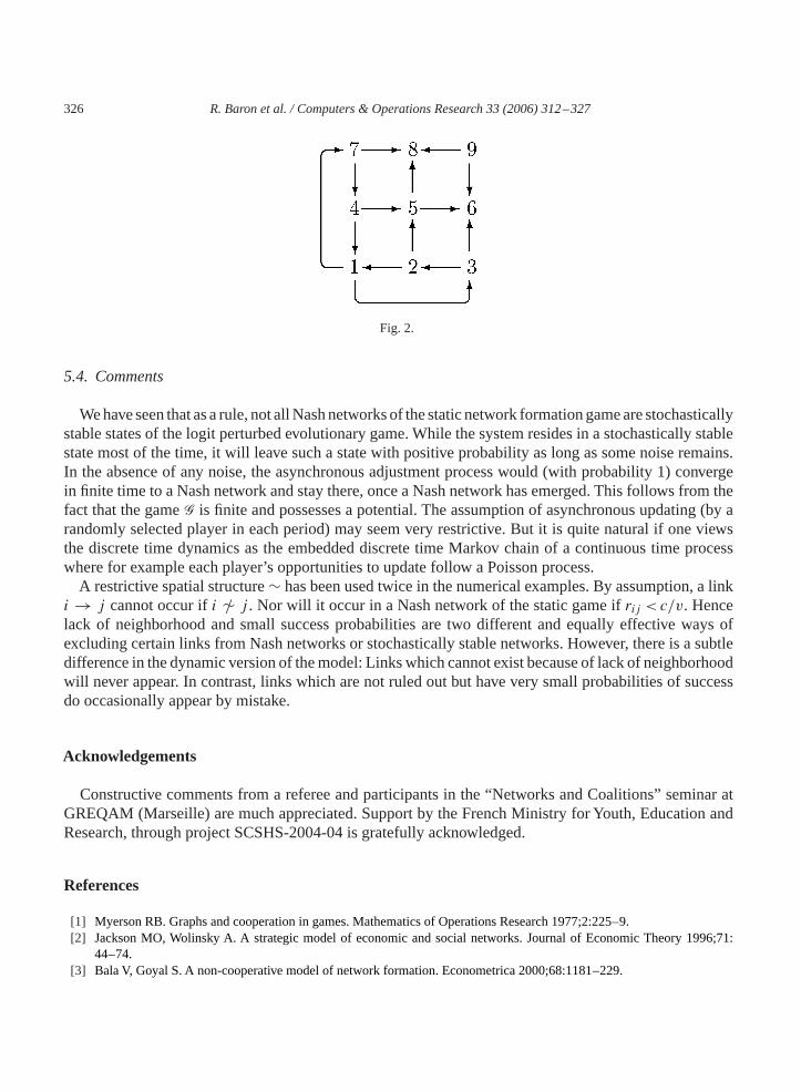
I are represented by the elements ofZ={1,2, . . . , m}2. In this representation,i= (i1, i2) for any playeri.We assume thatZ forms a finite torus and the neighborhood of a playeri is his vonNeumann neighborhoodon the torus, that isNi = {j : j1= i1± 1modm andj2= i2± 1modm}. Otherwise, we make the sameassumptions as in the very beginning of the example, so that each player wants to establish two singlelinks or no link at all. Let specificallyrij = 0.9 for all i �= j andKi(2)= 1.6 for all i so that the playerpopulation is homogeneous. Then there exist Nash networks where each player forms two single links,for instance the network which consists of the edgesi → j with j1= i1+ 1modm, j2= i2+ 1modm.These networks are stochastically stable. However, in general, there exist also Nash networks where notall players form two single links. Those networks are not stochastically stable. Form=3, such a networkis depicted inFig. 2. In this network, players 6 and 8 do not form links.When organizational costs are not of the formCi(si) = Ki(∑j sij ) for i ∈ I, si ∈ Si , analogous

(albeit somewhat more complicated) restrictions lead to the same Nash networks as in Example 2.However, determination of the stochastically stable networks proves more intricate without furtherrestrictions.

2 For largen and certain cost functionsKi , Nash networks may consist of a collection of stars.


Fig. 2.

5.4. Comments

Wehaveseen that asa rule, not all Nashnetworksof the static network formationgameare stochasticallystable states of the logit perturbed evolutionary game.While the system resides in a stochastically stablestate most of the time, it will leave such a state with positive probability as long as some noise remains.In the absence of any noise, the asynchronous adjustment process would (with probability 1) convergein finite time to a Nash network and stay there, once a Nash network has emerged. This follows from thefact that the gameG is finite and possesses a potential. The assumption of asynchronous updating (by arandomly selected player in each period) may seem very restrictive. But it is quite natural if one viewsthe discrete time dynamics as the embedded discrete time Markov chain of a continuous time processwhere for example each player’s opportunities to update follow a Poisson process.A restrictive spatial structure∼ has been used twice in the numerical examples. By assumption, a link

i → j cannot occur ifi /∼ j . Nor will it occur in a Nash network of the static game ifrij < c/v. Hencelack of neighborhood and small success probabilities are two different and equally effective ways ofexcluding certain links from Nash networks or stochastically stable networks. However, there is a subtledifference in the dynamic version of themodel: Links which cannot exist because of lack of neighborhoodwill never appear. In contrast, links which are not ruled out but have very small probabilities of successdo occasionally appear by mistake.

Acknowledgements

Constructive comments from a referee and participants in the “Networks and Coalitions” seminar atGREQAM (Marseille) are much appreciated. Support by the French Ministry for Youth, Education andResearch, through project SCSHS-2004-04 is gratefully acknowledged.

References

[1] Myerson RB. Graphs and cooperation in games. Mathematics of Operations Research 1977;2:225–9.[2] Jackson MO, Wolinsky A. A strategic model of economic and social networks. Journal of Economic Theory 1996;71:

44–74.[3] Bala V, Goyal S. A non-cooperative model of network formation. Econometrica 2000;68:1181–229.


[4] Baron R, Durieu J, Haller H, Solal P. A note on control costs and logit rules for strategic games. Journal of EvolutionaryEconomics 2002;12:563–75.

[5] Baron R, Durieu J, Haller H, Solal P. Control costs and potential functions for spatial games. International Journal of GameTheory 2002;31:541–61.

[6] Mattsson L-G, Weibull JW. Probabilistic choice and procedurally bounded rationality. Games and Economic Behavior2002;41:61–78.

[7] Monderer D, Shapley LS. Potential games. Games and Economic Behavior 1996;14:124–43.[8] Blume L. Statistical mechanics of strategic interaction. Games and Economic Behavior 1993;5:387–426.[9] Blume L. Population games. In: Arthur B, Durlauf S, Lane D., editors. The economy as an evolving complex systems II.

MA: AddisonWesley; 1997.[10] Young P. Individual strategy and social structure. Princeton, NJ: Princeton University Press; 1998.[11] Bala V, Goyal S. A strategic analysis of network reliability. Review of Economic Design 2000;5:205–28.[12] Haller H, Sarangi S. Nash networks with heterogeneous agents. Mimeo, Department of Economics, Virginia Polytechnic

Institute and State University, 2001.[13] Haller H. Large random graphs in pseudo-metric spaces. Mathematical Social Sciences 1990;20:147–64.[14] Johnson C, Gilles RP. Spatial social networks. Review of Economic Design 2000;5:273–99.[15] GareyMR, Johnson DS. Computers and intractability.A guide to the theory of NP-completeness. San Francisco: Freeman;

1979.[16] Garey MR, Johnson DS, Tarjan RE. The planar hamiltonian circuit problem is NP-complete. SIAM Journal of Computing

1976;5:704–14.[17] Ui TA. Shapley value representation of potential games. Games and Economic Behavior 2000;31:121–35.[18] Slikker M, Dutta D, van den Nouweland A, Tijs S. Potential maximizers and network formation. Mathematical Social

Sciences 2000;39:55–70.

Complexity and stochastic evolution of dyadic networks

Documents

Transcript of Complexity and stochastic evolution of dyadic networks