Complexity and self-organization inTuring

Jean Petitot∗

International Academy of Philosophy of Science ConferenceThe Legacy of A.M. Turing

Urbino, 25-28 september 2012

1 Introduction: “converting chemical information into a ge-ometrical form”

Alan Turing’s celebrated paper “The Chemical Basis of Morphogenesis” [22] pub-lished in 1952 in the Philosophical Transactions of the Royal Society of London isa typical example of a pioneering and inspired work in the domain of mathematicalmodelling.

1. The paper presents a new key idea for solving an old problem. As LionelHarrison said in his 1987 paper [6] “it is a theoretical preconception preceedingexperience”.

2. It contains right away the germ of quite the whole theory associated to thenew ideas.

3. Its forsightedness is striking. It anticipates by many years its experimentalconfirmations and mathematical developments.

The key idea is formulated from the outset in the first sentence:

“It is suggested that a system of chimical substances, called morphogens,reacting together and diffusing through a tissue, is adequate to accountfor the main phenomena of morphogenesis.”

∗CAMS, Ecole des Hautes Etudes en Sciences Sociale, Paris.e-mail : petitot@ehess.fr.fr

1

arX

iv:1

502.

0532

8v1

[q-

bio.

OT

] 1

8 Fe

b 20

15

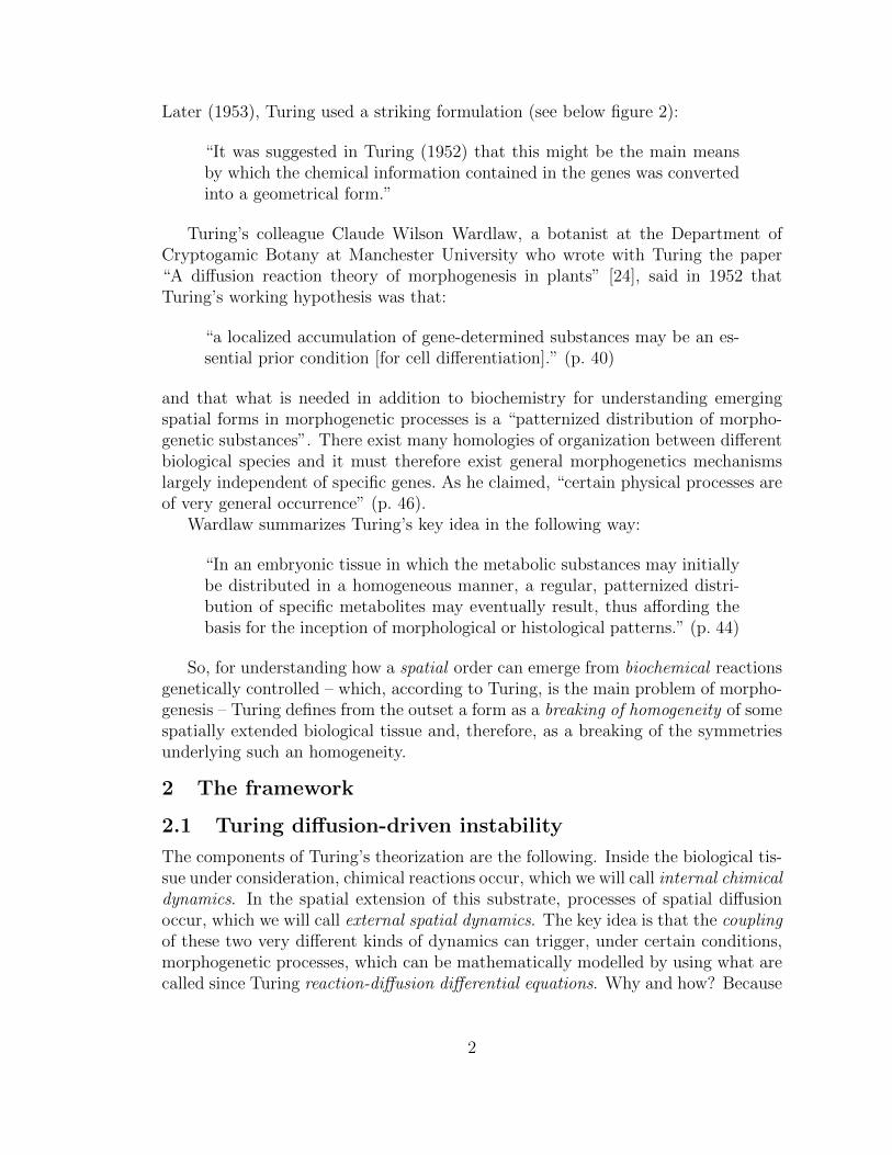
Later (1953), Turing used a striking formulation (see below figure 2):

“It was suggested in Turing (1952) that this might be the main meansby which the chemical information contained in the genes was convertedinto a geometrical form.”

Turing’s colleague Claude Wilson Wardlaw, a botanist at the Department ofCryptogamic Botany at Manchester University who wrote with Turing the paper“A diffusion reaction theory of morphogenesis in plants” [24], said in 1952 thatTuring’s working hypothesis was that:

“a localized accumulation of gene-determined substances may be an es-sential prior condition [for cell differentiation].” (p. 40)

and that what is needed in addition to biochemistry for understanding emergingspatial forms in morphogenetic processes is a “patternized distribution of morpho-genetic substances”. There exist many homologies of organization between differentbiological species and it must therefore exist general morphogenetics mechanismslargely independent of specific genes. As he claimed, “certain physical processes areof very general occurrence” (p. 46).

Wardlaw summarizes Turing’s key idea in the following way:

“In an embryonic tissue in which the metabolic substances may initiallybe distributed in a homogeneous manner, a regular, patternized distri-bution of specific metabolites may eventually result, thus affording thebasis for the inception of morphological or histological patterns.” (p. 44)

So, for understanding how a spatial order can emerge from biochemical reactionsgenetically controlled – which, according to Turing, is the main problem of morpho-genesis – Turing defines from the outset a form as a breaking of homogeneity of somespatially extended biological tissue and, therefore, as a breaking of the symmetriesunderlying such an homogeneity.

2 The framework

2.1 Turing diffusion-driven instability

The components of Turing’s theorization are the following. Inside the biological tis-sue under consideration, chimical reactions occur, which we will call internal chimicaldynamics. In the spatial extension of this substrate, processes of spatial diffusionoccur, which we will call external spatial dynamics. The key idea is that the couplingof these two very different kinds of dynamics can trigger, under certain conditions,morphogenetic processes, which can be mathematically modelled by using what arecalled since Turing reaction-diffusion differential equations. Why and how? Because

2

the external spatial diffusion can destabilize, under certain conditions, the internalchimical equilibria.

We must emphasize the fact that the notion of diffusion-driven instabilities is tosome extent paradoxical. Indeed, diffusion is a stabilizing process and therefore theidea amounts to posit that the coupling of two stabilities can induce an instability!

We will see that Turing assumes that there exists only one equilibrium of theinternal chimical dynamics. A diffusion-induced instability could therefore make thechimical state diverge, but in general non-linearities of the equations bound suchdivergences. Another possibility would be that there exist several equilibria. ThenTuring instabilities would induce bifurcations from one equilibrium state to anotherone. It is this idea that has been worked out in the late 1960s by Rene Thom [20],[21] to explain also morphogenesis.

2.2 Turing’s objective

Today, reaction-diffusion equations are mainly used to explain the formation of pat-terns in material substrates. But Turing’s objective was deeper and more ambitiousand concerned embryogenesis. As he claimed in his Introduction,

“The purpose of this paper is to discuss a possible mechanism by whichthe genes of a zygote may determine the anatomical structure of theresulting organism.” (p. 37)

As this general objective was too ambitious, he assumed many simplifications.The first simplification was to eliminate any direct reference to specific genes and toreduce the internal chemical dynamics to reaction equations between concentrationsof morphogens. As explains Philip Maini in [9], a morphogen is

“a chemical to which cells respond by differentiating in a concentration-dependent way.”

Turing was inspired by what Waddington [25] called “form producers” or “evoca-tors”. Morphogens are controlled by genes which catalize their production, but,contrary to genes, they can diffuse in the developing tissues and carry the positionalinformation (e.g. in the sense of Wolpert) which is needed for morphogenesis.1

The second simplification made by Turing was to eliminate the mechano-chemicalaspects of embryogenesis, although he was aware of their importance during thedevelopment. These aspects will be worked out later by specialists such as GeorgeOster and James Murray

But, even so drastically simplified, the search for good mathematical modelsremains a

“a problem of formidable mathematical complexity” (p. 38).

1For an introduction to the concept of “positional information” in Waddington, Wolpert, Good-win and Thom, see Petitot [18].

3

Figure 1: Turing’s general equation for morphogenesis.

Figure 2: Turing’s anticipation of the richness of the general equation for morpho-genesis.

In fact, it seems that Turing was looking for a kind of universal equation formorphogenesis. In his last paper “Morphogen theory of phyllotaxis”, which remainedunpublished because of his suicide and is kept at the King’s College Archives, heproposed the equation

dΓmdt

= µm∇2Γm + fm (Γ1, · · · ,ΓM)

where the Γm are the respective concentrations of the M morphogens, ∇2 the spatialLaplacian, that is the diffusion operator, the µm the diffusibility coefficients, andthe fm the reaction equations (see figure 1)

The point was that, when you vary the fm and the µm, the solutions of such auniversal equation can be extremely diverse (see figure 2). Hence the idea that, aswith Newton’s equation for Mechanics, it could be possible to classify a lot of verydifferent kinds of forms using the same general equation.

4

Indeed, we can vary three classes of parameters:

1. For the chemical part, the eigenvalues provided by the spectral analysis of thelinearized system of the fm.

2. The diffusibility coefficients µm.

3. For the geometrical part, the eigenfunctions of the Laplacian operator (har-monic analysis).

2.3 Turing’s foresightedness

In his 1990 paper “Turing’s theory of morphogenesis. Its influence on modellingbiological pattern and form” [15], James Murray claims that Turing’s 1952 paper is“one of the most important papers in theoretical biology of this century” (p. 119).Indeed,

“What is astonishing about Turing’s seminal paper is that, with veryfew exceptions, it took the mathematical world more than 20 years torealise the wealth of fascinating problems posed by his theory. What iseven more astonishing is that it was closer to 30 years before a significantnumber of experimental biologists took serious notice of its implicationsand potential applications in developmental biology, ecology and epi-demiology.” (p. 121)

These inspired anticipations proved to be exact in chemistry. There exist today alot of models of chimical reaction-diffusion phenomena: clocks, travelling waves, etc.Their analysis constitutes a rapidly expanding research domain while, at Turing’stime, no empirical example was known. Turing discovered theoretically the basicphenomenon and was the first to compute simulations on the computer he hadhimself constructed at Manchester. In embryogenesis, the exact limits of validity ofTuring model are still under discussion.

3 The context

3.1 The bibliography

It is interesting to look at Turing’s bibliography, which is very short. First, it in-cludes two books which are not really used, the Theory of Elasticity and Magnetismof James Jeans (1927) and The permeability of natural membranes of Hugh Dawsonand James Danielli (1943). Then, it cites a fundamental paper of Leonor Michaelisand Maud Menten (1913) on Die Kinetik der Invertinwirkung [13] whose pioneeringmathematical model is typical of the internal chimical dynamics used by Turing.Finally, there are three masterpieces on embryology and morphogenesis: CharlesManning Child’s “summa” Patterns and problems of development (1941), Sir D’Arcy

5

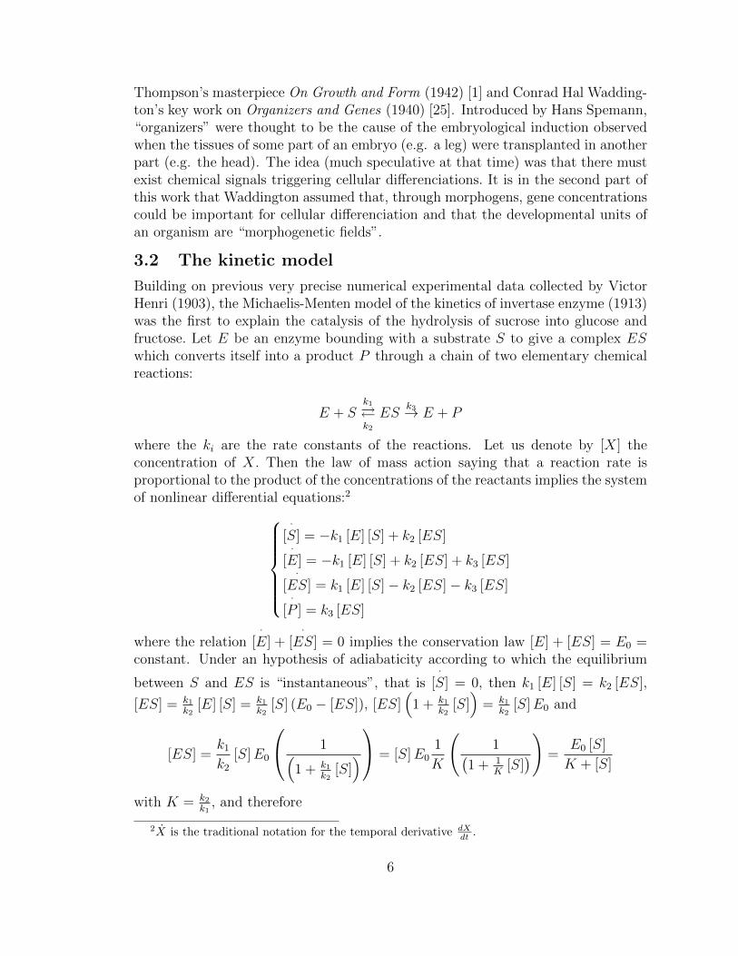
Thompson’s masterpiece On Growth and Form (1942) [1] and Conrad Hal Wadding-ton’s key work on Organizers and Genes (1940) [25]. Introduced by Hans Spemann,“organizers” were thought to be the cause of the embryological induction observedwhen the tissues of some part of an embryo (e.g. a leg) were transplanted in anotherpart (e.g. the head). The idea (much speculative at that time) was that there mustexist chemical signals triggering cellular differenciations. It is in the second part ofthis work that Waddington assumed that, through morphogens, gene concentrationscould be important for cellular differenciation and that the developmental units ofan organism are “morphogenetic fields”.

3.2 The kinetic model

Building on previous very precise numerical experimental data collected by VictorHenri (1903), the Michaelis-Menten model of the kinetics of invertase enzyme (1913)was the first to explain the catalysis of the hydrolysis of sucrose into glucose andfructose. Let E be an enzyme bounding with a substrate S to give a complex ESwhich converts itself into a product P through a chain of two elementary chemicalreactions:

E + Sk1�k2

ESk3→ E + P

where the ki are the rate constants of the reactions. Let us denote by [X] theconcentration of X. Then the law of mass action saying that a reaction rate isproportional to the product of the concentrations of the reactants implies the systemof nonlinear differential equations:2

·[S] = −k1 [E] [S] + k2 [ES]·

[E] = −k1 [E] [S] + k2 [ES] + k3 [ES]·

[ES] = k1 [E] [S]− k2 [ES]− k3 [ES]·

[P ] = k3 [ES]

where the relation·

[E] +·

[ES] = 0 implies the conservation law [E] + [ES] = E0 =constant. Under an hypothesis of adiabaticity according to which the equilibrium

between S and ES is “instantaneous”, that is·

[S] = 0, then k1 [E] [S] = k2 [ES],

[ES] = k1k2

[E] [S] = k1k2

[S] (E0 − [ES]), [ES](

1 + k1k2

[S])

= k1k2

[S]E0 and

[ES] =k1k2

[S]E0

1(1 + k1

k2[S]) = [S]E0

1

K

(1(

1 + 1K

[S])) =

E0 [S]

K + [S]

with K = k2k1

, and therefore

2X is the traditional notation for the temporal derivative dXdt .

6

·[P ] = k3

E0 [S]

K + [S]

4 Turing’s numerical example

So, Turing start with morphogens diffusing and reacting inside a tissue. Diffusionflows from regions of strong concentrations towards regions of weak concentrationswith a velocity proportional to the gradients of the concentrations and to the dif-fusibility coefficients. According to the law of mass action, reaction rates are propor-tional to the product of concentrations. Hence a huge variety of nonlinear differentialequations.

Turing gives several examples and develop one of them in minute detail in his§10 “A numerical example”. He considers a ring of N = 20 cells and two mor-phogens X and Y and makes several numerical assumptions on their size, the dif-fusibility constants, the permeability of membranes (it is here that the reference toDawson-Danielli is used), etc. With great acuity, he argues that the system mustbe (thermodynamically) open and include a “fuel substance” A providing it withenergy through its degradation into another substance B.

“In order to maintain the wave pattern a continual supply of free energyis required. It is clear that this must be so since there is a continualdegradation of energy through diffusion. This energy is supplied throughthe ‘fuel substances’ (A, B in the last example), which are degraded into‘waste products’.” (p. 65)

For modelling catalysis, Turing add three other substances C, C ′, and W .It must be emphasized that it will be only thirty years later that open thermo-

dynamical systems out of equilibrium will be systematically investigated (see e.g.Prigogine’s dissipative structures).

4.1 The internal chimical dynamics

The system of 7 elementary reactions proposed by Turing is the following:

[1]Y +X → W rate: 2516XY

[2]W + A→ 2Y +B(instantly)A = 1000 = constant (fuel substance)

[3] 2X → W rate: 764X2

[4]A→ X rate: 116

10−3A = 116

[5]Y → B rate: 116Y

[6]Y + C → C ′(instantly)C = C ′ = 10−3 (1 + γ)

[7]C ′ → X + C rate: 5532

103C ′ = 5532

(1 + γ)

So, X converts into Y at the rate 132

[50XY + 7X2 − 55 (1 + γ)] (because of [1],[3], and [7]) while self-reproducing (because of [4]) at the constant rate 1

16and

7

destroying Y (because of [5]) at the rate 116Y . So the kinetic equations for the

time varying concentrations X (t), Y (t) of the morphogens X, Y – i.e. the internalchimical dynamics – are{ ·

X = 132

[−50XY − 7X2 + 57 + 55γ] = f (X, Y )·Y = 1

32[50XY + 7X2 − 55− 55γ − 2Y ] = g (X, Y )

where 57 in the first equation is 55 + 2 with 2 coming from [4] and −2Y in thesecond equation comes from [5].

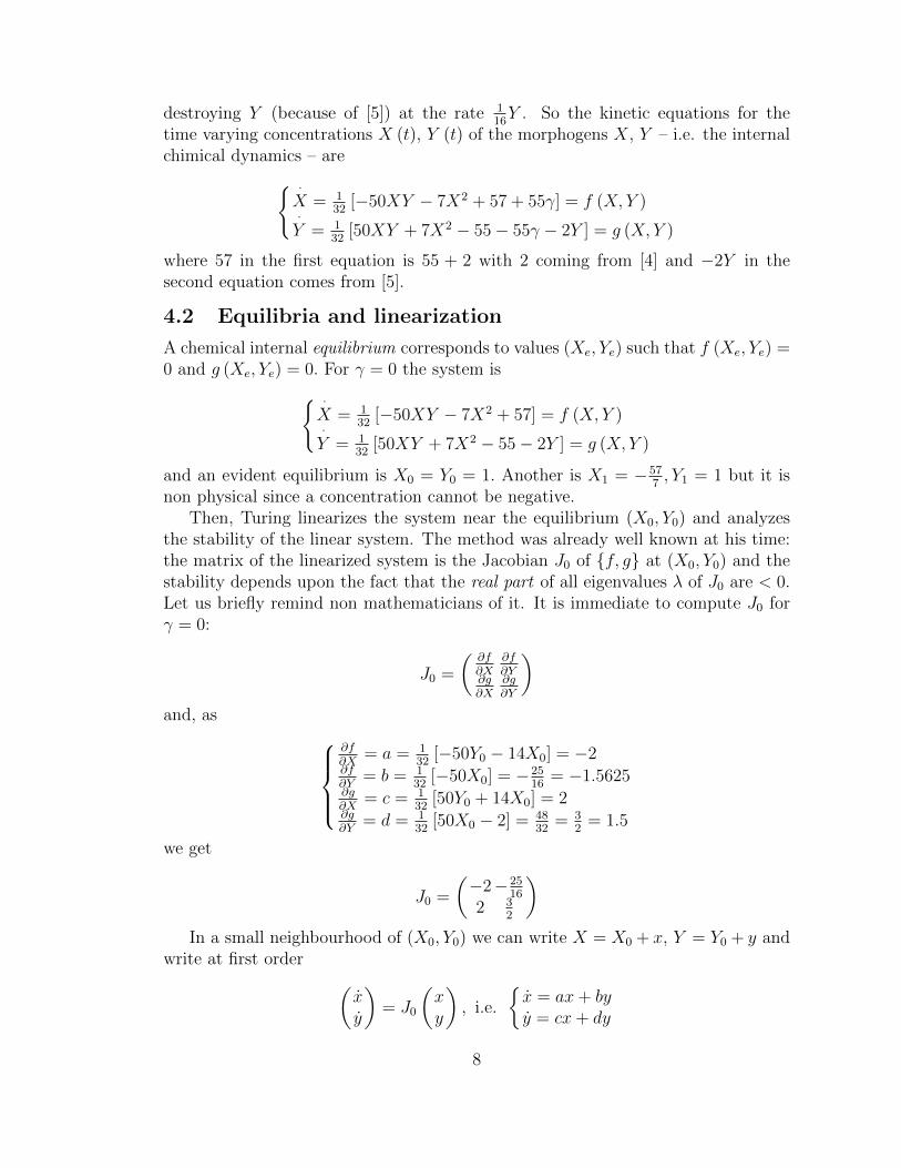
4.2 Equilibria and linearization

A chemical internal equilibrium corresponds to values (Xe, Ye) such that f (Xe, Ye) =0 and g (Xe, Ye) = 0. For γ = 0 the system is{ ·

X = 132

[−50XY − 7X2 + 57] = f (X, Y )·Y = 1

32[50XY + 7X2 − 55− 2Y ] = g (X, Y )

and an evident equilibrium is X0 = Y0 = 1. Another is X1 = −577, Y1 = 1 but it is

non physical since a concentration cannot be negative.Then, Turing linearizes the system near the equilibrium (X0, Y0) and analyzes

the stability of the linear system. The method was already well known at his time:the matrix of the linearized system is the Jacobian J0 of {f, g} at (X0, Y0) and thestability depends upon the fact that the real part of all eigenvalues λ of J0 are < 0.Let us briefly remind non mathematicians of it. It is immediate to compute J0 forγ = 0:

J0 =

(∂f∂X

∂f∂Y

∂g∂X

∂g∂Y

)and, as

∂f∂X

= a = 132

[−50Y0 − 14X0] = −2∂f∂Y

= b = 132

[−50X0] = −2516

= −1.5625∂g∂X

= c = 132

[50Y0 + 14X0] = 2∂g∂Y

= d = 132

[50X0 − 2] = 4832

= 32

= 1.5

we get

J0 =

(−2−25

16

2 32

)In a small neighbourhood of (X0, Y0) we can write X = X0 + x, Y = Y0 + y and

write at first order (xy

)= J0

(xy

), i.e.

{x = ax+ byy = cx+ dy

8

As the system is linear, we look at solutions of the form(x (t)y (t)

)= eλt

(x0y0

)where (x0, y0) is the state of the system at time t = 0. They are straight trajecto-ries on the line (0, 0) − (x0, y0) with an exponential temporal law. Computing thederivatives in two different ways, we get(

xy

)= J0

(xy

)= λeλt

(x0y0

)= λ

(xy

)that is an equation linking λ to J0:

(J0 − λI)

(xy

)= 0

If (x0, y0) 6= (0, 0), then (x, y) 6= (0, 0) and this equation can be satisfied only if thedeterminant Det (J0 − λI) vanishes. The equation Det (J0 − λI) = 0 is called thecharacteristic equation of the linear system. It is a polynomial equation of degree 2which writes

Det

(a− λ bc d− λ

)= 0

λ2 − (a+ d)λ+ ad− bc= 0

λ2 − Tr (J0)λ+ Det (J0) = 0

λ2 − Sλ+ P = 0

where the sum of diagonal terms Tr (J0) = a + d = S, called the trace of thematrix J0, gives the sum S of the solutions and the determinant Det (J0) of J0gives their product P . As the discriminant of the equation is ∆ = S2 − 4P =Tr (J0)

2 − 4 Det (J0), the solutions are given by the well known formula

λ±=1

2

(S ±√

∆)

λ±=1

2

(Tr (J0)±

√Tr (J0)

2 − 4 Det (J0)

)and any solution of the linear system is a linear combination of the two solutionswith λ±.

Let us suppose now that λ = α + iω has real part Re (λ) = α and imaginarypart Im (λ) = ω. Then, eλt = e(α+iω)t = eαteiωt is an oscillation modulated bythe real exponential eαt. If α > 0, eαt diverges exponentially when t → +∞ andthe corresponding trajectories go to infinity and are unstable. On the contrary, if

9

α < 0, eαt converges exponentially towards 0 when t→ +∞ and the correspondingtrajectories go to equilibrium and are stable. In Turing’s example,

Tr (J0) = a+ d = −2 +3

2= −1

2

Det (J0) = ad− bc = −2× 3

2−(−25

16

)× 2 =

1

8

λ±=−1

4(1± i) , Re (λ±) = −1

4< 0

and the two eigenvalues have negative real parts. The internal chemical equilibrium(X0, Y0) (i.e. (x0, y0) = 0) is therefore stable.

More generally, in the 2-dimensional case, the system is stable if and only if{Tr (J0) = a+ d < 0, here − 1

2< 0

Det (J0) = ad− bc > 0, here 18> 0

Indeed, we must have Re (λ±) < 0. If ∆ = Tr (J0)2 − 4 Det (J0) < 0, then λ+ and

λ− are complex conjugate eigenvalues and we must have Tr (J0) < 0, and of courseDet (J0) > 0 because otherwise we would have ∆ > 0. If ∆ ≥ 0, then λ+ and λ− arereal eigenvalues and they must be both < 0. This imply that the greatest eigenvalue,namely λ+ = Tr (J0)+

√∆ must be < 0, which implies Tr (J0) < −

√∆. So Tr (J0) <

0, and, as Tr (J0)2 > ∆ = Tr (J0)

2 − 4 Det (J0), we have also Det (J0) > 0.

5 Diffusion-driven instability

After having defined the internal chemical equilibrium and analyzed its stability,Turing explains how a spatial diffusion of the morphogens X, Y can induce aninstability. Let us summarize his computations.

5.1 The reaction-diffusion model

Let r = 1, · · · , N label the positions of the N cells in the ring. ConcentrationsX, Y are then functions X(r, t) and Y (r, t) of time t and spatial position r. In acontinuous model, the spatial positions would be parametrized by an angle θ ∈ S1

and concentrations would be functions X(θ, t) and Y (θ, t) (angles θr = 2π rN

retrievethe discrete case). We start with an homogeneous initial state where X(r, t) = X0

and Y (r, t) = Y0 everywhere and we apply diffusion using the Laplace operator∆ = ∇2 and its discrete approximation ∆F (r) = F (r − 1)− 2F (r) + F (r + 1) forany function F (r).

We get that way the reaction-diffusion equations·X(r, t) = f (X(r, t), Y (r, t)) +

µ (X(r − 1, t)− 2X(r, t) +X(r + 1, t))·Y (r, t) = g (X(r, t), Y (r, t)) +

ν (Y (r − 1, t)− 2Y (r, t) + Y (r + 1, t))

, (r = 1, . . . , N)

10

where µ and ν are the respective coefficients of diffusibility of X and Y . Sometechnical aspects of the general analysis of such equations are well emphasized byTuring in §11 “Restatement and biological interpretation of the results” (p. 66),with an incredible sense of anticipation: it is essential to take into account

1. the role of fluctuations, which play a critical role when the system becomesunstable;

2. the role of slow changes of reaction rates and diffusibility coefficients because“such changes are supposed ultimately to bring the system out of the stablestate”.

Turing considered therefore that the systems he analyzed belong to the class ofwhat are called today slow-fast dynamical systems and focused on the breaking ofspatial homogeneity near instability. As he said

“the phenomena when the system is just unstable were the particularsubject of the inquiry.”

He underlined the fact that the “linearity assumption” near the equilibrium, i.e.the fact that the dynamics is qualitatively equivalent to its linear part, is “a seriousone” and made what is called today an hypothesis of adiabaticity : as the system isa slow-fast one, the slow variation of parameters is slow w.r.t. the fast time used toreach equilibrium and, therefore, one can suppose that the system is always in itsequilibrium state until he reaches a bifurcation destabilizing it.

In terms of the variables x (r, t) and y (r, t), the linearized reaction-diffusionequations are:

·x(r, t) = ax(r, t) + by(r, t)+

µ (x(r − 1, t)− 2x(r, t) + x(r + 1, t))·y(r, t) = cx(r, t) + dy(r, t)+

ν (y(r − 1, t)− 2y(r, t) + y(r + 1, t))

, (r = 1, . . . , N)

In the continuous limit on a circle of radius 1, they are(x (θ, t)y (θ, t)

)= J0

(x (θ, t)y (θ, t)

)+

(µ′ 00 ν ′

)(x′′ (θ, t)y′′ (θ, t)

)where x′′ and y′′ are spatial second derivatives (Laplacian term).

A pedagogical interest of the ring model is that the space is the circle S1, thatthe eigenfunctions of the Laplacian are the trigonometric functions, and that theharmonic analysis is therefore nothing else than Fourier analysis. Let ξ (s, t) andη (s, t) be the Fourier tranforms of x (r, t) and y (r, t):{

ξ (s, t) = 1N

∑r=Nr=1 exp

(−2πirs

N

)x(r, t)

η (s, t) = 1N

∑r=Nr=1 exp

(−2πirs

N

)y(r, t)

, (r = 1, . . . , N)

11

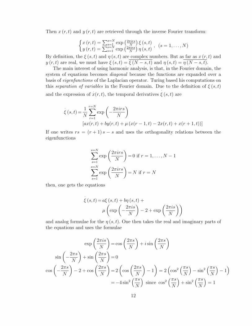
Then x (r, t) and y (r, t) are retrieved through the inverse Fourier transform:{x (r, t) =

∑s=Ns=1 exp

(2πirsN

)ξ (s, t)

y (r, t) =∑s=N

s=1 exp(2πirsN

)η (s, t)

, (s = 1, . . . , N)

By definition, the ξ (s, t) and η (s, t) are complex numbers. But as far as x (r, t) andy (r, t) are real, we must have ξ (s, t) = ξ (N − s, t) and η (s, t) = η (N − s, t).

The main interest of using harmonic analysis, is that, in the Fourier domain, thesystem of equations becomes diagonal because the functions are expanded over abasis of eigenfunctions of the Laplacian operator. Turing based his computations onthis separation of variables in the Fourier domain. Due to the definition of ξ (s, t)

and the expression of·x(r, t), the temporal derivatives

·ξ (s, t) are

·ξ (s, t) =

1

N

r=N∑r=1

exp

(−2πirs

N

)[ax(r, t) + by(r, t) + µ (x(r − 1, t)− 2x(r, t) + x(r + 1, t))]

If one writes rs = (r + 1) s − s and uses the orthogonality relations between theeigenfunctions

s=N∑s=1

exp

(2πirs

N

)= 0 if r = 1, . . . , N − 1

s=N∑s=1

exp

(2πirs

N

)=N if r = N

then, one gets the equations

·ξ (s, t) = aξ (s, t) + bη (s, t) +

µ

(exp

(−2πis

N

)− 2 + exp

(2πis

N

))and analog formulae for the η (s, t). One then takes the real and imaginary parts ofthe equations and uses the formulae

exp

(2πis

N

)= cos

(2πs

N

)+ i sin

(2πs

N

)sin

(−2πs

N

)+ sin

(2πs

N

)= 0

cos

(−2πs

N

)− 2 + cos

(2πs

N

)= 2

(cos

(2πs

N

)− 1

)= 2

(cos2

(πsN

)− sin2

(πsN

)− 1)

=−4 sin2(πsN

)since cos2

(πsN

)+ sin2

(πsN

)= 1

12

to get the equations{ ·ξ (s, t) =

(a− 4µ sin2

(πsN

))ξ (s, t) + bη (s, t)

·η (s, t) = cξ (s, t) +

(d− 4ν sin2

(πsN

))η (s, t)

In the continuous model, the Fourier transforms of functions on S1 are Fourierseries whose components are indexed by k ∈ Z and one gets{ ·

ξ (k, t) = (a− µ′k2) ξ (k, t) + bη (k, t)·η (k, t) = cξ (k, t) + (d− ν ′k2) η (k, t)

with k2 corresponding to N2

π2 sin2(πsN

). Turing denotes by U this variable.

5.2 The origin of instability

The fundamental new phenomenon introduced by diffusion is that the spectral anal-ysis of the linearized system now depends upon diffusion which, by changing thecharacteristic equation, can tranform eigenvalues with Re (λ) < 0 into eigenvalueswith Re (λ) > 0. It is the origin of diffusion-driven instabilities. Indeed, the Jacobianis now

J =

(a− 4µ sin2

(πsN

)b

c d− 4ν sin2(πsN

))and the characteristic equation – also called a dispersion relation – is therefore(

p− a+ 4µ sin2(πsN

))(p− d+ 4ν sin2

(πsN

))= bc

Turing denotes by ps and p′s, with Re (ps) ≥ Re (p′s) the two eigenvalues. Ifps 6= p′s then the solutions of the system in the Fourier domain are of the form{

ξ (s, t) = Asepst +Bse

p′st

η (s, t) = Csepst +Dse

p′st

If ps and p′s are real, then AN−s = As, etc. If ps and p′s are conjugate complexnumbers, then BN−s = As, etc. It is straightforward to verify that the coefficientssatisfy the relations: {

As(ps − a+ 4µ sin2

(πsN

))= bCs

Bs

(p′s − a+ 4µ sin2

(πsN

))= bDs

Now if Max (Re (ps)) > 0, some diverging Fourier modes will become dominantand push the system out of equilibrium. Such a possibility can happen only underprecise conditions relating the parameters a, b, c, d of the internal chemical equilib-rium to the parameters µ, ν of the external spatial diffusion. Turing explains verywell that generically only a single Fourier mode (with its conjugate) can becomedominant. Indeed, if it was not the case,

13

“the quantities a, b, c, d, µ, ν will be restricted to satisfy some specialcondition, which they would be unlikely to satisfy by chance.” (p. 50)

Let s0 be the index yielding Max (Re (ps)) and suppose Re (ps0) > 0. If the twoeigenvalues ps0 and p′s0 are real, the pair (ps0 , pN−s0) will induce divergences since

sin2(π(N−s0)

N

)= sin2

(πs0N

), and if they are complex conjugate the two pairs (ps0 , pN−s0)

and(p′s0 , p

′N−s0

)will both induce divergences.

6 A toy model

Turing presents a simple numerical example p. 52. The parameters are

a= I − 2, b = 2.5, c = −1.25, d = I + 1.5

µ′= 1, ν ′ =1

2,µ

µ′=ν

ν ′=

(N

2πρ

)2

, U =

(N

πρ

)2

sin2(πsN

)The characteristic equation is therefore

(p− a+ 4µ sin2

(πsN

))(p− d+ 4ν sin2

(πsN

))= bc(

p− I + 2 + 4

(N

2πρ

)2

sin2(πsN

))(p− I − 1.5 + 2

(N

2πρ

)2

sin2(πsN

))= bc

(p− I + 2 + U)

(p− I − 1.5 +

1

2U

)+ (2.5) (1.25) = 0

(p− I)2 +

(1

2+

3

2U

)(p− I) +

1

2

(U − 1

2

)2

= 0

We observe that p = I for U = 12. Let sc be the corresponding value of s. If the radius

ρ of the ring is such that there exists an integer s0 satisfying U =(Nπρ

)2sin2

(πs0N

)=

12, then there will exist stationary waves with s0 lobes. Otherwise, it will be the s0

nearest to sc which will dominate.The figure 3 displays for I = 0 the graph Γ of the hyperbola p2 +

(12

+ 32U)p +

12

(U − 1

2

)2= 0 in the (U, p) plane for U ∈ [0, 1.2] and p ∈ [−0.4, 0], and I = 0.

The points of Γ are evident. If p is considered as a parameter,

U =1

2

(1− 3p±

√p2 − 10p

)and if U is considered as a parameter,

p =1

4

(−1− 3U ±

√U2 + 14U − 1

).

14

0.0 0.2 0.4 0.6 0.8 1.0 1.2

-0.4

-0.3

-0.2

-0.1

0.0

Figure 3: The graph Γ of p2 +(12

+ 32U)p + 1

2

(U − 1

2

)2= 0 for U ∈ [0, 1.2] and

p ∈ [−0.4, 0].

The solutions of U2 + 14U − 1 = 0 are U = −7 ± 5√

2 but, as U is a real square(Nπρ

)2sin2

(πsN

), the only admissible value is Uc = −7 + 5

√2 ∼ 0.071 and for Uc the

two values of p are equal to −14

(1 + 3U) ∼ 0.30325. For U > Uc, the two p roots are

real and for 0 ≤ U < Uc, they have an imaginary part Im (p) = ±√U2 + 14U − 1

while the real part move on the segment Re (p) = −14

(1 + 3U) from the point(U = 0, p = −1

4

)to the point (U ∼ 0.071, p ∼ 0.30325). In what concerns p, as U

is real, we must have√p2 − 10p real, that is p2 − 10p ≥ 0 i.e. p ∈ (−∞, 0] or

p ∈ [10,+∞).The figure 4 reproduces Turing’s figure 1 which displays Re (p) and − |Im (p)| as

functions of U for I = 0.

7 Conditions for instability and the critical point

In the §9 “Further considerations on the mathematics of the ring”, Turing analyzesfurther the conditions under which a diffusion-driven instability can occur. We willpresent and complete his computations using the continuous model which is easierto understand.

As reaction-diffusion equations are linear, and since every function on S1 is alinear superposition of harmonics eikθ, we look at solutions of the form(

xy

)= eλteikθ

(x0y0

)

15

Figure 4: Turing’s figure 1 which displays Re (p) and − |Im (p)| as functions of U forI = 0. The full line and the dotted line represent respectively Re (ps) and Re (p′s),while the broken line represents − |Im (p)|. Turing has indicated with black thickpoints the integer values from s = 0 (left) to s = 5 (right).

which implies immediately

(xy

)= λeλteikθ

(x0y0

)=

J0eλteikθ

(x0y0

)+

(µ′ 00 ν ′

)(−k2eλteikθ

)(x0y0

), that is

(J0 − k2D − λI

)(xy

)= 0, with D =

(µ′ 00 ν ′

)The characteristic equation is therefore

Det(J0 − k2D − λI

)= Det

(a− µ′k2 − λ b

c d− ν ′k2 − λ

)= 0

and the dispersion relations are(λ− a+ µ′k2

) (λ− d+ ν ′k2

)= bc

or, if we write this equation λ2 − S (k2)λ + P (k2) = 0 with S (k2) the sum of itstwo roots and P (k2) their product,

λ2 −(Tr (J0)− k2 Tr (D)

)λ+

(µ′ν ′k4 − (ν ′a+ µ′d) k2 + Det (J0)

)= 0

We want Tr (J0) = a + d < 0 and Det (J0) = ad− bc > 0 to ensure the stabilityof the internal chemical equilibrium. But we want also one λ with Re (λ) > 0

16

to ensure a diffusion-driven instability. As Tr (J0) < 0 and Tr (D) = µ′ + ν ′ >0, this implies S (k2) = Tr (J0) − k2 Tr (D) < 0. If P (k2) happened to be > 0,we would have two roots with Re (λ) < 0, so we must have P (k2) < 0. But asDet (J0) > 0 by hypothesis and of course µ′ν ′k4 > 0, we need in fact ν ′a + µ′d >µ′ν ′k2 + Det (J0) /k

2 > 0. This is a first condition. As Tr (J0) = a + d < 0 andµ′, ν ′ > 0, we need µ′ 6= ν ′ since, if µ′ and ν ′ would be equal, we would haveν ′a+ µ′d = µ′ (a+ d) < 0.

It is essential to strongly emphasize here the fact that the diffusibility of the twomorphogens X and Y must be sufficiently different in order that an instability canoccur. It is the key of Turing’s discovery.

In the example of §10, µ′ = α 12, ν ′ = α 1

4(α > 0), a = −2, d = 3

2and the

condition ν ′a+ µ′d = α(−2× 1

4+ 3

2× 1

2

)= α

4> 0 is therefore satisfied.

There is a second condition. P (k2) = µ′ν ′k4−(ν ′a+ µ′d) k2+Det (J0) is a seconddegree polynomial in k2 and we want it to become < 0 for values of k2 which mustnecessarilly be positive since k2 is a real square. Let δ = µ′

ν′. The graph of P (k2) is

a parabola Π starting at Det (J0) > 0 for k = 0. If δ < δc for a critical value to becomputed, Π is over the k2-axis and the condition P (k2) < 0 cannot be satisfied.But if δ > δc, Π intersects the k2-axis at two points k21 and k22 > k21 and inside theinterval [k21, k

22] the condition P (k2) < 0 is satisfied: there exists an eigenvalue λ

with Re (λ) > 0.The computation of δc is rather tedious. Let u = k2. The polynomial P (u) and

its first and second derivatives are

P (u) =µ′ν ′u2 − (ν ′a+ µ′d)u+ ad− bcP ′ (u) =− (ν ′a+ µ′d) + 2µ′ν ′u

P ′′ (u) = 2µ′ν ′

So the minimum of Π is given by P ′ (u) = − (ν ′a+ µ′d) + 2µ′ν ′u = 0 and it is aminimum since P ′′ (u) = 2µ′ν ′ > 0. Its value is

u0 = k20 =ν ′a+ µ′d

2µ′ν ′

and we have

P(k20)

= ad− bc− 1

4

(ν ′a+ µ′d)2

µ′ν ′

For P (k2) to become < 0, we must have therefore

0 < ad− bc < 1

4

(ν ′a+ µ′d)2

µ′ν ′=

1

4

(a+ δd)2

δ

and δc is given by the equation

17

ad− bc =1

4

(a+ δcd)2

δc

In the example, when γ = 0, we have ad− bc = 18, ν ′a+ µ′d = α

4, µ′ν ′ = α2

8, and

we verify that 18

= 14×(14

)2× 8. So Turing’s system is at its critical point for γ = 0.Let us now investigate more precisely the second degree equation giving δc. It

can be written

d2δ2c + 2 (2bc− ad) δc + a2 = 0

and its two solutions are

δc± =ad− 2bc± 2

√−bc (ad− bc)

d2

But as one root, and hence both roots, must be real, we need −bc (ad− bc) > 0 and,as ad− bc > 0 by hypothesis, we must have bc < 0.

In the example, for γ = 0, we have effectively −2516× 2 < 0 and

δc =

(1

32

)2[

1

8−(−25

16× 2

)+ 2

√(25

16

)×(

1

8

)]= 2 = δ

As δ = δc we are indeed at the critical point. Then

P(k2)

=α2

8k4 − α

4k2 +

1

8=

1

8

(αk2 − 1

)2and the parabola Π is tangent at the k2-axis and at the point of tangency theeigenvalues are λ+ = 0 and λ = Tr (J0)− k2 Tr (D) = −

(3α4k2)− 1

2< 0. So, at the

crossing of the critical point, the eigenvalue λ+ becomes > 0.

8 The bifurcation

After having analyzed the conditions of a diffusion-driven instability at a criticalpoint, Turing analyzed further the behavior of the system in the neighbourhood ofthe critical point. To this end, he varied the small parameter γ around its criticalvalue γ = 0. Today, computations are very easy, but at his time they were difficultand he must use the computer he had himself constructed. We will first do themfor the continuous model and then return to Turing’s own discrete model.

8.1 Continuous model

The chemical internal equilibrium is now given by the concentrations of morphogens

X0 =1

7

(−25 +

√210 + 7× 55γ

), Y0 = 1

18

1 2 3 4 5

-0.2

0.2

0.4

0.6

0.8

1.0

1.2

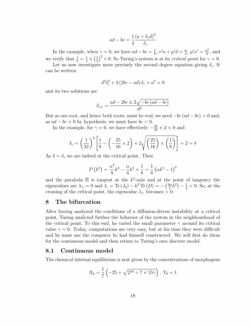
Figure 5: The graph of P (k2) for ε = 0.1. Inside the interval [0.367, 2.862] of k2 wehave P (k2) < 0.

We linearize the system in the neighbourhood of (X0, Y0) and compute first orderexpansions in the small parameter ε = 7×55

210γ = 385

1024γ. We get

a = −2− ε, b = −25

16− 25

7ε, c = 2 + ε, d =

3

2+

25

7ε

and the conditions for instability: Tr (J0) = a + d = −12

+ 187ε must be < 0, which

implies ε < 736∼ 0.194; ν ′a + µ′d = 1

4+ 43

28ε must be > 0, which implies ε > − 7

43;

Det (J0) = ad− bc = 18

+ 116ε must be > 0, which implies ε > −2; ad must be < 0,

which implies ε > − 42121

; ad− bc must be < 14(ν′a+µ′d)2

µ′ν′, which implies ε > 0.

The equation yielding the eigenvalues is now

λ2 −(Tr (J0)− k2 Tr (D)

)λ+ P

(k2)

= 0

Figure 5 displays the graph of P (k2) for ε = 0.1. The roots of P (k2) = 0 are0.367 and 2.862 and inside their interval we have P (k2) < 0.

The characteristic equation is

λ2 −(Tr (J0)− k2 Tr (D)

)λ+

(µ′ν ′k4 − (ν ′a+ µ′d) k2 + Det (J0)

)= 0

that is

λ2 +

(1

2+

3k2

4− 18

7ε

)λ+

(k4

8−(

1

4+

43

28ε

)k2 +

1

8+

1

16ε

)= 0

and its roots λ± are approximated by

1

128

(−7 + 36ε±

√−49− 553ε+ 1296ε2 + 490k2 − 308εk2 + 343k4

)Figures 7 and 9 display the graphs of λ+ and λ (including the irrelevant negativek2-axis). For λ+ we see that λ+ ≥ 0 for k2 ∈ [0.367, 2.862]. Figure 8 zooms on

19

-2.0 -1.5 -1.0 -0.5 0.5 1.0

-200

200

400

600

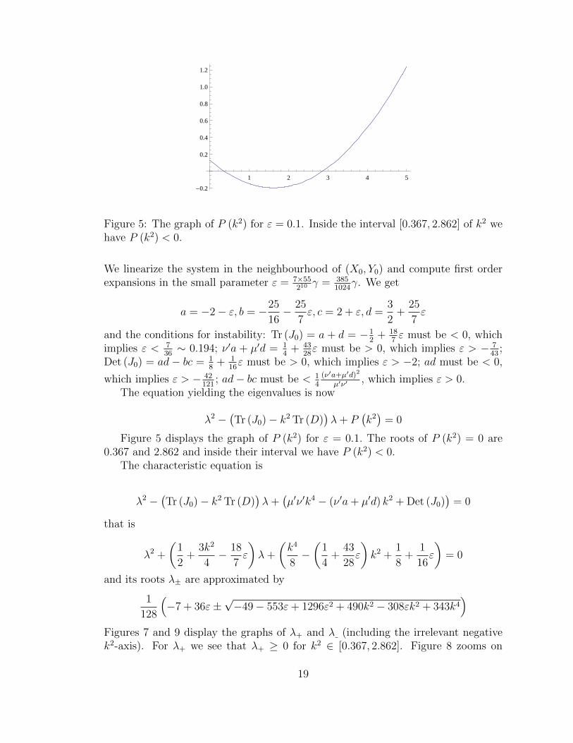
Figure 6: The discriminant ∆ (k2) for ε = 0.1. ∆ is negative inside the open interval]−1.5146, 0.1758[ .

-10 -5 5 10

2

4

6

8

10

12

Figure 7: Graph of λ+ (including the irrelevant negative k2-axis). λ+ ≥ 0 fork2 ∈ [0.367, 2.862]. There is no graph inside the open interval ]−1.5146, 0.1758[where the discriminant ∆ of the characteristic equation is < 0.

this interval. There is no graph inside the open interval ]−1.5146, 0.1758[ where thediscriminant ∆ of the characteristic equation is < 0 (see figure 6).

8.2 Discrete model

Let us come back to the discrete ring model composed of N = 20 cells. At thecritical point γ = 0, the 20 characteristic equations in the Fourier domain are(

p+ 2 + 2 sin2(πs

20

))(p− 1.5 + sin2

(πs20

))+

25

8= 0

The figure 10 shows the table of the 20 pairs (ps, p′s) of eigenvalues for s = 0, . . . , 19.

We see that if we order the p w.r.t to increasing Re (p) we get p3 = p17 = −0.00346,p4 = p16 = −0.012, p5 = p15 = −0.064, p2 = p18 = −0.066. It is therefore the modep3 which can most readily become > 0.

20

1 2 3 4 5

-0.25

-0.20

-0.15

-0.10

-0.05

0.05

Figure 8: Zoom on the interval k2 ∈ [0.367, 2.862] of the figure 7 where λ+ ≥ 0.

-10 -5 5 10

-10

-5

Figure 9: Graph of λ (including the irrelevant negative k2-axis). λ is always < 0for k2 > 0. There is no graph inside the open interval ]−1.5146, 0.1758[ where thediscriminant ∆ of the characteristic equation is < 0.

eq@s_D := Hp + 2 + 2 * HSin@Pi * s � 20DL^2L * Hp - 1.5 + HSin@Pi * s � 20DL^2L + 25 � 8 == 0;Table@Solve@eq@sD, pD, 8s, 0, 19<D888p -> -0.25 - 0.25 I<, 8p -> -0.25 + 0.25 I<<,

88p -> -0.286708 - 0.139731 I<, 8p -> -0.286708 + 0.139731 I<<,88p -> -0.720177<, 8p -> -0.0662972<<,88p -> -1.11487<, 8p -> -0.00345613<<, 88p -> -1.52451<, 8p -> -0.0119627<<,88p -> -1.93541<, 8p -> -0.0645857<<, 88p -> -2.32263<, 8p -> -0.140898<<,88p -> -2.65919<, 8p -> -0.222488<<, 88p -> -2.92013<, 8p -> -0.293399<<,88p -> -3.08537<, 8p -> -0.341218<<, 88p -> -3.14194<, 8p -> -0.358059<<,88p -> -3.08537<, 8p -> -0.341218<<, 88p -> -2.92013<, 8p -> -0.293399<<,88p -> -2.65919<, 8p -> -0.222488<<, 88p -> -2.32263<, 8p -> -0.140898<<,88p -> -1.93541<, 8p -> -0.0645857<<, 88p -> -1.52451<, 8p -> -0.0119627<<,88p -> -1.11487<, 8p -> -0.00345613<<, 88p -> -0.720177<, 8p -> -0.0662972<<,88p -> -0.286708 - 0.139731 I<, 8p -> -0.286708 + 0.139731 I<<<

Figure 10: The table of the 20 pairs (ps, p′s) of eigenvalues of the discrete ring model

for s = 0, . . . , 19 and γ = 0.

21

eq2@s_D :=

Hp + 2.02336 + 2 * HSin@Pi * s � 20DL^2L * Hp - 1.58344 + HSin@Pi * s � 20DL^2L � -1.64594 * 2.02336list2 = Table@Solve@eq2@sD, pD, 8s, 0, 19<D888p ® -0.21996 - 0.279424 ä<, 8p ® -0.21996 + 0.279424 ä<<,

88p ® -0.256668 - 0.183836 ä<, 8p ® -0.256668 + 0.183836 ä<<,88p ® -0.673699<, 8p ® -0.0526953<<,88p ® -1.0807<, 8p ® 0.0224553<<, 88p ® -1.49637<, 8p ® 0.0199735<<,88p ® -1.9113<, 8p ® -0.0286193<<, 88p ® -2.30143<, 8p ® -0.102014<<,88p ® -2.64011<, 8p ® -0.181492<<, 88p ® -2.90249<, 8p ® -0.25096<<,88p ® -3.06857<, 8p ® -0.297935<<, 88p ® -3.12542<, 8p ® -0.314498<<,88p ® -3.06857<, 8p ® -0.297935<<, 88p ® -2.90249<, 8p ® -0.25096<<,88p ® -2.64011<, 8p ® -0.181492<<, 88p ® -2.30143<, 8p ® -0.102014<<,88p ® -1.9113<, 8p ® -0.0286193<<, 88p ® -1.49637<, 8p ® 0.0199735<<,88p ® -1.0807<, 8p ® 0.0224553<<, 88p ® -0.673699<, 8p ® -0.0526953<<,88p ® -0.256668 - 0.183836 ä<, 8p ® -0.256668 + 0.183836 ä<<<

Figure 11: The table of the 20 pairs (ps, p′s) of eigenvalues of the discrete ring model

for s = 0, . . . , 19 and γ = 116

.

Let us now vary the small slow parameter γ. Turing varied γ almost adiabaticallyfrom −1

4(stability) to 1

16(instability) at speed γ = 2−7 = 1

128. This corresponds

to variations ε : −0.094 → 0.0235 for ε and t : 0 → 40 for the discrete time t.For γ = −1

4, the equilibrium is (X0 = 0.78, Y0 = 1), and a0 = −1.9, b0 = −1.218,

c0 = 1.9, d0 = 1.156, and all Re (ps) < 0: the system is stable. On the contrary, forγ = − 1

16, the equilibrium is (X1 = 1.053, Y1 = 1), and a1 = −2.023, b1 = −1.646,

c1 = 2.023, d1 = 1.583, and p3 = p17 = 0.0224 > 0, p4 = p16 = 0.012 > 0: the systemis unstable. The figure 11 shows the table of the 20 pairs (ps, p

′s) of eigenvalues for

s = 0, . . . , 19 for γ = 116

.In figure 12 we show the 20 graphs Re (ps) as functions of t for γ varying from

−14

to 116

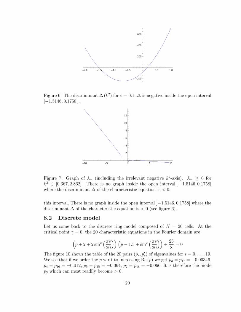
. The time t varies from t = 0 to t = 40. We see the Re (ps) which become> 0 for s = 3, 17, 4, 16. At t = 40, p3 = p17 = 0.0224 and p4 = p16 = 0.012. Fors = 0, 1, 19, Re (ps) presents an angular point because ps is a complex number withIm (ps) 6= 0. It is the same phenomenon as in the toy model of figure 4. Figure 13shows the graphs of Re (p) and Im (p) in such a case.

In his paper, Turing computes (with his recently constructed Manchester com-puter) the table of the evolution of the ring (see figure 14) and shows how Fouriermodes become dominant after the bifurcation induced by the diffusion-driven insta-bility (see figure 15). In the initial state, all cells are, up to small fluctuations, inthe equilibrium state (X0 = 1, Y0 = 1). After the bifurcation, a stationary oscilla-tory wave pattern with 3 lobes develops. The divergences induced by the instabilityare tamed by two factors: (i) the concentration X cannot become < 0 and whenX (r, t) vanishes, the process stops locally, (ii) saturation non-linear effects allow anew equilibrium to occur. These results constitute a great achievement.

9 Further aspects of Turing’s paper

In his paper, Turing evoked many other problems. In §4 he gave simple examplesfor explaining the idea of “breakdown of symmetry and homogeneity” in pattern

22

Figure 12: The 20 graphs Re (ps) as functions of t for γ varying from −14

to 116

. Thetime t varies from t = 0 to t = 40. The Re (ps) become > 0 for s = 3, 17, 4, 16. Att = 40, p3 = p17 = 0.0224 and p4 = p16 = 0.012. For s = 0, 1, 19, Re (ps) presentsan angular point because ps is a complex number with Im (ps) 6= 0. It is the samephenomenon as in the toy model of figure 4.

23

10 20 30 40

-0.4

-0.3

-0.2

-0.1

0.1

0.2

0.3

Figure 13: When Im (p) 6= 0 (graph up), Re (p) (graph down) presents an angularpoint.

Figure 14: Turing’s computation of the evolution of the ring.

24

Figure 15: The evolution of the ring after the bifurcation induced by a diffusion-driven instability. The hatched graph represents the X concentration at the initialstate: all cells are, up to small fluctuations, in the equilibrium state (X0 = 1, Y0 = 1).The other graph represents a stationary oscillatory wave pattern with 3 lobes. Thedivergences induced by the stability are tamed by two factors: (i) the concentrationX cannot become < 0, (ii) non-linear effects.

25

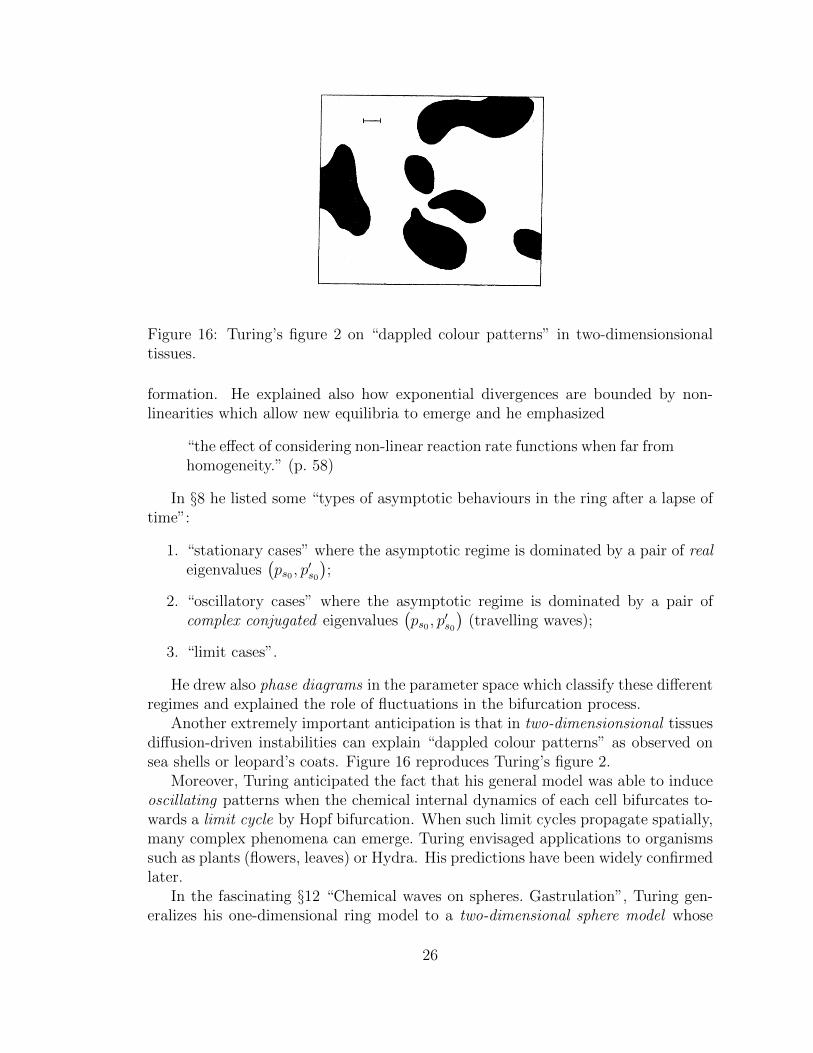
Figure 16: Turing’s figure 2 on “dappled colour patterns” in two-dimensionsionaltissues.

formation. He explained also how exponential divergences are bounded by non-linearities which allow new equilibria to emerge and he emphasized

“the effect of considering non-linear reaction rate functions when far fromhomogeneity.” (p. 58)

In §8 he listed some “types of asymptotic behaviours in the ring after a lapse oftime”:

1. “stationary cases” where the asymptotic regime is dominated by a pair of realeigenvalues

(ps0 , p

′s0

);

2. “oscillatory cases” where the asymptotic regime is dominated by a pair ofcomplex conjugated eigenvalues

(ps0 , p

′s0

)(travelling waves);

3. “limit cases”.

He drew also phase diagrams in the parameter space which classify these differentregimes and explained the role of fluctuations in the bifurcation process.

Another extremely important anticipation is that in two-dimensionsional tissuesdiffusion-driven instabilities can explain “dappled colour patterns” as observed onsea shells or leopard’s coats. Figure 16 reproduces Turing’s figure 2.

Moreover, Turing anticipated the fact that his general model was able to induceoscillating patterns when the chemical internal dynamics of each cell bifurcates to-wards a limit cycle by Hopf bifurcation. When such limit cycles propagate spatially,many complex phenomena can emerge. Turing envisaged applications to organismssuch as plants (flowers, leaves) or Hydra. His predictions have been widely confirmedlater.

In the fascinating §12 “Chemical waves on spheres. Gastrulation”, Turing gen-eralizes his one-dimensional ring model to a two-dimensional sphere model whose

26

geometry is more complex, the harmonic analysis on the sphere resting on the eigen-functions of the spherical Laplacian, namely the spherical harmonics. His strikingidea was to apply the model to gastrulation in embryology, which is the step at whichthe spherical symmetry of the blastula is broken. He developed this idea further inhis unpublished paper on phyllotaxis.

Finally, in the last §13 “Non-linear theory. Use of digital computer”, Turing cameback to the assumption that linearization is a good approximation and explainedthat it is the case only in the neighbourhood of the first bifurcation. It is

“an assumption which is justifiable in the case of a system just beginningto leave a homogeneous condition.” (p. 72)

For Turing it was risky to try to go beyond:

“One cannot hope to have any very embracing theory of such processes,beyond the statement of the equations.” (p. 73)

Hence the fundamental interest of the just constructed digital computers enablingnumerical simulations avoiding the too drastic simplifications imposed by the searchof explicit theoretical solutions to the equations.

10 Conclusion: after Turing

To conclude this presentation of Turing’s 1952 paper, let us look briefly at the workson reaction-diffusion equations after Turing. I have already tackle this theme in mytalk [19] at the IAPS 2001 Conference on Complexity and Emergence.

10.1 General reaction-diffusion models

Among the many specialists of the domain, we would cite Hans Meinhardt andAlfred Gierer who, since 1972 [5], have considerably increased our knowledge onreaction-diffusion models. They have shown that, for an activator/inhibitor pair ofmorphogens, instabilities mainly result from the competition between a short rangeslow activation and a long range fast inhibition, the inhibitor diffusing faster thanthe excitator. This confirms Turing’s remark on the role of the difference betweenthe two diffusibility coefficients µ and ν.

A general Meinhardt-Gierer model has the form{x = ρx

2

y− αx+ σx + µ∆x

y = ρx2 − βy + σy + ν∆yα < β, µ� ν

The activator morphogen x is self-catalizing (x2 term in x) and its production isinhibited by the inhibitor morphogen y ( 1

yterm in x). Moreover, x catalyzes its

inhibitor (x2 term in y). The linear terms αx and βy (α < β) are degradation terms,the constant σy enables a stable homogeneous state and the constant σx allows totrigger the process. µ and ν are the diffusibility coefficients with µ (slow) � ν

27

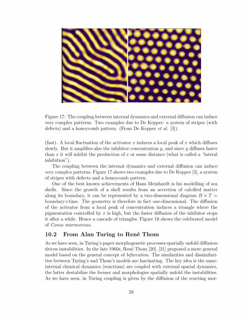
Figure 17: The coupling between internal dynamics and external diffusion can inducevery complex patterns. Two examples due to De Kepper: a system of stripes (withdefects) and a honeycomb pattern. (From De Kepper et al. [3]).

(fast). A local fluctuation of the activator x induces a local peak of x which diffusesslowly. But it amplifies also the inhibitor concentration y, and since y diffuses fasterthan x it will inhibit the production of x at some distance (what is called a “lateralinhibition”).

The coupling between the internal dynamics and external diffusion can inducevery complex patterns. Figure 17 shows two examples due to De Kepper [3], a systemof stripes with defects and a honeycomb pattern.

One of the best known achievements of Hans Meinhardt is his modelling of seashells. Since the growth of a shell results from an accretion of calcified matteralong its boundary, it can be represented by a two-dimensional diagram B × T =boundary×time. The geometry is therefore in fact one-dimensional. The diffusionof the activator from a local peak of concentration induces a triangle where thepigmentation controlled by x is high, but the faster diffusion of the inhibitor stopsit after a while. Hence a cascade of triangles. Figure 18 shows the celebrated modelof Conus marmoreous.

10.2 From Alan Turing to Rene Thom

As we have seen, in Turing’s paper morphogenetic processes spatially unfold diffusion-driven instabilities. In the late 1960s, Rene Thom [20], [21] proposed a more generalmodel based on the general concept of bifurcation. The similarities and dissimilari-ties between Turing’s and Thom’s models are fascinating. The key idea is the same:internal chimical dynamics (reactions) are coupled with external spatial dynamics,the latter destabilize the former and morphologies spatially unfold the instabilities.As we have seen, in Turing coupling is given by the diffusion of the reacting mor-

28

Figure 18: Meinhardt’s model for the sea shell Conus marmoreous. In front a trueshell. In the background its reaction-diffusion model. (From Meinhardt [10]).

phogens. In Thom, coupling is more generally a spatial control of internal dynamicsand the morphogenetic discontinuities breaking the homogeneity of the substrateare induced by bifurcations.

10.3 Beyond Turing

After Turing, many authors, e.g. James Murray [14], [15], introduced bifurcationsin reaction-diffusion equations. Let u be the vector (x, y) and consider a differentialequation u = f (u, r) where r is a spatial control. When r varies and crosses a criticalvalue rc, the initial stable equilibrium state u0 of the system can collapse with anunstable equilibrium and disappear. The system is therefore projected to anotherequilibrium through this saddle-node bifurcation. Another most used bifurcationis the Hopf bifurcation. When r varies and crosses a critical value rc, the initialstable (i.e. attracting) equilibrium state u0 becomes a repellor and generates asmall attracting closed orbit (i.e. a limit cycle).

Consider for instance the following system analyzed by Robin Engelhardt [4]:{x = −xy2 + ay − (1 + b)x+ δ∆xy = xy2 − (1 + a) y + x+ F + δ∆y

The chemical internal equilibria without diffusion (δ = 0) are solutions of the equa-tions (if y2 + 1 + b 6= 0):

29

x =ay

y2 + 1 + b

ay3

y2 + 1 + b− (1 + a) y +

ay

y2 + 1 + b+ F = 0

that is

y3 − Fy2 + (1 + b+ ab) y − F (1 + b) = 0

which is a cubic equation with parameters a, b, F .At the points where y2 + 1 + b = 0, we have{

x = ay + δ∆xy = −bx− (1 + a) y + F + δ∆y

and this can be an equilibrium point for δ = 0 only if ay = 0 and −bx− y + F = 0.If a 6= 0, this implies the condition b = −1, and the equilibrium is y = 0, x = −F .If a = 0, the equilibrium would be −bx− y + F = 0 with y2 + 1 + b = 0. Figure 19shows some examples of patterns solution of this system of equations.

There is a wealth of material on these topics. The reader could look e.g. atHarrison [6], Lee et al. [7], [8], Maini [9], Oyang-Swinney [16], or Pearson [17].

10.4 Experimental results

The validity of Turing’s models for embryology are still under discussion. But inwhat concerns chimical and biological patterns their validity is without doubt. Wehave seen Meinhardt’s examples. For chemical systems exact verifications go backto 1990 and the works of the Bordeaux group of Patrick De Kepper (Castets, Du-los, Boissonade) on iodate-ferrocyanide-sulfite or clorite-iodide-malonic acid-starchreactions in gel reactors.

It is a full universe of morphological phenomena and mathematical models thatTuring opened in 1952 with a remarkable foresightedness.

References

[1] D’Arcy Thompson, 1942. On Growth and Form, Cambridge University Press,Cambridge.

[2] V. Castets, E. Dulos, J. Boissonade, P. De Kepper, 1990. “Experimental evi-dence of a sustained standing Turing type non-equilibrium chemical pattern”,Physical Review Letter, 64 (1990) 2953-2955.

[3] P. De Kepper et al. 1998. “Taches, rayures et labyrinthes”, La Recherche, 305,84-89.

[4] R. Engelhardt, 1994. Modelling Pattern Formation in Reaction-Diffusion Sys-tems, Thesis, University of Copenhagen.

30

Figure 19: Some examples of patternized solutions of Engelhardt’s system of equa-tions. (From [4]).

31

[5] A. Gierer, H. Meinhardt, 1972. “A theory of biological pattern formation”,Kybernetik, 12 (1972) 30-39.

[6] L.G. Harrison, 1987.“What is the status of reaction-diffusion theory thirty-fouryears after Turing?”, Journal of Theoretical Biology, 125 (1987) 369-384.

[7] K.J. Lee, W.D. McCormick, Q. Ouyang, H.L. Swinney, 1993. “Pattern Forma-tion by Interacting Chemical Fronts”, Science, 261 (1993) 192-194.

[8] K.J. Lee, W.D. McCormick, J.E. Pearson, H.L. Swinney, 1994. “ExperimentalObservation of Self-replicating Spots in a Reaction-diffusion System”, Nature,369 (1994) 215-218.

[9] P. Maini, 2012. “Turing’s mathematical theory of morphogenesis, Asia PacificMathematics Newsletter, 2, 1 (2012) 7-8.

[10] H. Meinhardt, 1982. Models of Biological Pattern Formation, Academic Press,London.

[11] H. Meinhardt, P. Prusinkiewicz, D. Fowler, 2003. The Algorithmic Beauty ofSea Shells, Springer, Berlin, 2003.

[12] H. Meinhardt, 2012. “Turing’s theory of morphogenesis of 1952 and the sub-sequent discovery of the crucial role of local self-enhancement and long-rangeinhibition, Interface Focus, 2, 4 (2012) 407-416.

[13] L. Michaelis, M. Menthen, 1913. “Die Kinetic der Invertin-wirkung”, Biochemische Zeitschrift, 49 (1913) 333-369. Engl. transl.R.S. Goody, K.A. Johnson, “The Kinetics of Invertase Action”,http://path.upmc.edu/divisions/chp/PDF/Michaelis-Menten Kinetik.pdf.

[14] J.D. Murray, 1989. Mathematical Biology. An Introduction, Springer, Berlin.[15] J.D. Murray, 1990. “Turing’s theory of morphogenesis. Its influence on mod-

elling biological pattern and form”, Bulletin of Mathematical Biology, 52, 1/2(1990) 119-152.

[16] Q. Oyang, H.L. Swinney, 1991. “Transition from a uniform state to hexagonaland striped Turing patterns”, Nature, 352 (1991) 610-612.

[17] J.E. Pearson, 1993. “Complex Patterns in a Simple System”, Science, 261(1993) 189-192.

[18] J. Petitot, 2003. Morphogenesis of Meaning, Peter Lang, Bern.[19] J. Petitot, 2003. “Modeles de structures emergentes dans les systemes com-

plexes”, Complexity and Emergence (E. Agazzi, L. Montecucco eds), Proceed-ings of the Annual Meeting of the International Academy of the Philosophy ofScience, World Scientific, Singapore, 57-71.

[20] R. Thom, 1972. Stabilite structurelle et morphogenese, Intereditions, Paris.[21] R. Thom, 1974. Modeles mathematiques de la morphogenese, Collection 10/18,

Union Generale d’Editions, Paris.[22] A.M. Turing, 1952. “The Chemical Basis of Morphogenesis”, Philosophical

Transactions of the Royal Society of London, Series B, Biological Sciences,237, 641(1952) 37-72.

[23] A.M. Turing, 1953. “Morphogen Theory of Phyllotaxis”, King’s College ArchiveCenter, Cambrige (unpublished).

32

[24] A.M. Turing, C.W. Wardlaw, 1952. “A diffusion reaction theory of morphogen-esis in plants”, New Phyt. 52, 40-47. Also in Collected Works of A.M. Turing,P.T. Saunders, Amsterdam, 1953, 37-47.

[25] C.H. Waddington, 1940. Organizers and Genes, Cambridge University Press,Cambridge.

33