Complexity and performance of temperature -based snow ... · 1 Complexity and performance of...
31
1 Complexity and performance of temperature-based snow routines for runoff modelling in mountainous areas in Central Europe Marc Girons Lopez 1, 2 , Marc J. P. Vis 1 , Michal Jenicek 3 , Nena Griessinger 4 , Jan Seibert 1 1 Department of Geography, University of Zurich, Zurich, CH-8006, Switzerland 2 Swedish Meteorological and Hydrological Institute, Norrköping, SE-60176, Sweden 5 3 Department of Physical Geography and Geoecology, Charles University, Prague, CZ-11636, Czechia 4 WSL Institute for Snow and Avalanche Research SLF, Davos, CH-7260, Switzerland Correspondence to: Marc Girons Lopez ([email protected]) Abstract. Snow processes are a key component of the water cycle in mountainous areas as well as in many areas of the mid- and high latitudes of the Earth. The complexity of these processes, coupled with the limited data available on them, has led 10 to the development of different modelling approaches to improve their understanding and support management practices. Physically-based approaches, such as the energy balance method, provide the best representation of these processes but at the expense of high data requirements. Data limitations, in most situations, constrain the use of these methods in favour of more simple approaches. The temperature-index method is the most widely-used modelling approach of the snowpack processes for hydrological modelling, with many variants implemented in different models. However, in many cases, the 15 decisions on the most suitable complexity of these conceptualisations are not adequately assessed for a given model structure, application, or decision-making support tool. In this study, we assessed model structure choices of the HBV model, a popular semi-distributed, bucket-type hydrological model, for its application in mountainous areas in Central Europe. To this end, we reviewed the most widely-used choices to different components of the snow routine in different hydrological models and proposed a series of modifications to the 20 structure of HBV. We constrained the choice of modifications to those that are aligned with HBV’s modelling approach of keeping processes as simple as possible to constrain model complexity. We analysed a total of 64 alternative snow routine structures over 54 catchments using a split-sample test. We found that using (a) an exponential snowmelt function coupled with no refreezing instead of a linear function for both processes and (b) a seasonally-variable degree-day factor instead of a constant one were, overall, the most valuable modifications to the model. Additionally, we found that increasing model 25 complexity does not necessarily lead to improved model performance per se. Instead, we found that a thorough analysis of the different processes included in the model and their optimal degree of realism for a given application is a preferable alternative. While the results may not be transferrable to other modelling purposes or geographical domains, the methodology presented here may be used to assess the suitability of model design choices. https://doi.org/10.5194/hess-2020-57 Preprint. Discussion started: 13 February 2020 c Author(s) 2020. CC BY 4.0 License.
Transcript of Complexity and performance of temperature -based snow ... · 1 Complexity and performance of...

1
Complexity and performance of temperature-based snow routines
for runoff modelling in mountainous areas in Central Europe
Marc Girons Lopez1, 2, Marc J. P. Vis1, Michal Jenicek3, Nena Griessinger4, Jan Seibert1
1Department of Geography, University of Zurich, Zurich, CH-8006, Switzerland 2Swedish Meteorological and Hydrological Institute, Norrköping, SE-60176, Sweden 5 3Department of Physical Geography and Geoecology, Charles University, Prague, CZ-11636, Czechia 4WSL Institute for Snow and Avalanche Research SLF, Davos, CH-7260, Switzerland
Correspondence to: Marc Girons Lopez ([email protected])
Abstract. Snow processes are a key component of the water cycle in mountainous areas as well as in many areas of the mid-
and high latitudes of the Earth. The complexity of these processes, coupled with the limited data available on them, has led 10
to the development of different modelling approaches to improve their understanding and support management practices.
Physically-based approaches, such as the energy balance method, provide the best representation of these processes but at
the expense of high data requirements. Data limitations, in most situations, constrain the use of these methods in favour of
more simple approaches. The temperature-index method is the most widely-used modelling approach of the snowpack
processes for hydrological modelling, with many variants implemented in different models. However, in many cases, the 15
decisions on the most suitable complexity of these conceptualisations are not adequately assessed for a given model
structure, application, or decision-making support tool.
In this study, we assessed model structure choices of the HBV model, a popular semi-distributed, bucket-type hydrological
model, for its application in mountainous areas in Central Europe. To this end, we reviewed the most widely-used choices to
different components of the snow routine in different hydrological models and proposed a series of modifications to the 20
structure of HBV. We constrained the choice of modifications to those that are aligned with HBV’s modelling approach of
keeping processes as simple as possible to constrain model complexity. We analysed a total of 64 alternative snow routine
structures over 54 catchments using a split-sample test. We found that using (a) an exponential snowmelt function coupled
with no refreezing instead of a linear function for both processes and (b) a seasonally-variable degree-day factor instead of a
constant one were, overall, the most valuable modifications to the model. Additionally, we found that increasing model 25
complexity does not necessarily lead to improved model performance per se. Instead, we found that a thorough analysis of
the different processes included in the model and their optimal degree of realism for a given application is a preferable
alternative. While the results may not be transferrable to other modelling purposes or geographical domains, the
methodology presented here may be used to assess the suitability of model design choices.
https://doi.org/10.5194/hess-2020-57Preprint. Discussion started: 13 February 2020c© Author(s) 2020. CC BY 4.0 License.

2
1 Introduction 30
Snow is an essential aspect of the seasonal hydrological variations in Alpine areas as well as in many other regions of the
mid and high latitudes of the Earth. Unlike rainfall, which contributes directly to groundwater recharge and stream runoff,
snowfall accumulates on the ground creating a temporary freshwater reservoir. This accumulated water is then gradually
released through melting, often triggered by raising temperatures, and ultimately contributes to runoff. The snow
accumulated on the ground (i.e. snowpack) is not only crucial for ecological reasons (Hannah et al., 2007), but also for many 35
human activities such as hydropower, agriculture, or tourism (Barnett et al., 2005). At the same time, snow processes can
also lead to risks for society. For instance, the accumulation of snow on steep slopes may, under the right conditions, cause
avalanches (Schweizer et al., 2003) and the sudden melt of large amounts of snow, such as during rain-on-snow events (Sui
and Koehler, 2001) or after rapid increases of air temperature, may lead to widespread flooding either directly (Merz and
Blöschl, 2003) or indirectly (e.g. dam failure accidents) (Rico et al., 2008). 40
Society´s dependence on the freshwater stored in the snowpack and its vulnerability to its associated risks raises the need to
understand its dynamics and evolution (Fang et al., 2014; Jamieson and Stethem, 2002). Nevertheless, even if knowledge on
snow hydrology has broadly advanced over the last decades, the limitations of data availability on catchment hydrology –
and especially on snow processes – pose a challenge to properly monitoring these processes as well as implementing
adequate management policies and practices. Furthermore, the evolution of snow water resources in the future cannot be 45
estimated through direct observation, but is essential in the context of global climate change (Berghuijs et al., 2014; Jenicek
and Ledvinka, 2020).
Consequently, different modelling strategies have been developed to overcome the data limitations and to study the
evolution of the snowpack and its impact on water resources. The most common modelling approaches are based either on
the physically-based energy budget model or on the temperature-index distribution function method (Verdhen et al., 2014). 50
While energy budget models are the most accurate alternative to represent snowpack processes, in order to be reliable they
usually require data that are often not available in conventional meteorological stations (Avanzi et al., 2016). These models
attempt to estimate the snow contribution to runoff in a distributed way by solving the energy balance of the snowpack,
which requires detailed data on topography, temperature, wind speed and direction, cloud cover fraction, snow density, etc.
Conversely, temperature-based models tend to have low data requirements and offer a balance between simplicity and 55
realism, which makes them successful in many different contexts and applications, even in cases with limited data
availability (Hock, 2003). Hybrid methods have also been developed, such as including a radiation component in the
temperature-based models (Hock, 1999). These approaches are especially relevant for high elevation, often glacierised areas
in which temperature seldom gets above the freezing point (Gabbi et al., 2014; Pellicciotti et al., 2005).
The temperature-index model – also referred to as degree-day method – is based on the observation that the rate of snowmelt 60
is proportional to the temperature above the freezing point per unit time through a proportionality constant commonly named
degree-day factor (Collins, 1934; Martinec, 1960). Many distribution function hydrological models use variations of this
https://doi.org/10.5194/hess-2020-57Preprint. Discussion started: 13 February 2020c© Author(s) 2020. CC BY 4.0 License.

3
method to simulate snowpack processes. For instance, while some models use the freezing point as reference temperature
(Walter et al., 2005), others include a calibrated threshold temperature parameter (Viviroli et al., 2007). Regarding the
proportionality constant, some applications define it as time-independent (Valéry et al., 2014), while others establish it as 65
being seasonally-variable (Hottelet et al., 1994). Moreover, connecting with energy budget models, some applications use
two proportionality constants: one for temperature and another for net radiation (Kane et al., 1997). Nevertheless, regardless
of the preferred approach, the inherent simplifications made in semi-distributed temperature-index models leave out some
critical aspects of the snowpack processes that may be significant in some circumstances. For instance, the disregard of
lateral transport processes may lead to the development of unreasonable accumulations of snow over long periods of time 70
(i.e., snow towers) in high mountainous areas (Freudiger et al., 2017; Frey and Holzmann, 2015).
The different implementations of the temperature-index method may relate to differences in model philosophy, scope,
desired resolution, or available computing power, among others. Nevertheless, these choices are not always adequately
tested to ensure that they provide the best possible alternative for a given model design and application (Harpold et al.,
2017). For instance, some studies have found that a more realistic representation of hydrological processes does not always 75
translate into improved model performance (Orth et al., 2015). For a long time, limitations in computing power hindered the
systematic testing of different alternative model structures over a large number of catchments. In recent years, however, the
increase in computing power has made these tests not only feasible but also desirable in order to ensure that model structures
are adequate and robust for their intended applications (Günther et al., 2019).
In this study, we evaluated the design choices made in the snow routine of the HBV hydrological model (Bergström, 1995), 80
a typical bucket-type model with a temperature-based snow routine, for its application in mountainous central-European
catchments. We implemented and tested a number of modifications to the snow routine of the model based on common
practices in similar hydrological models, and investigated whether it is possible to identify model structure alternatives
which generally result in improved model performance. With this, we aimed to provide a basis to decide on useful
modifications to the model while avoiding adding unnecessary complexity and additional parameters. To ensure that the 85
results are representative we explored different levels of added complexity, from single modifications to combinations of
multiple modifications, to a large dataset of catchments covering a wide range of climatological and hydrological conditions
of the area of interest.
2 Materials and Methods
The HBV model is a bucket-type rainfall-runoff model, with a number of boxes (routines) including the main components of 90
the terrestrial phase of the water cycle, i.e., snow routine, soil routine, groundwater (response) routine, and routing function.
In this study, we focus solely on the snow routine of the model. We use the HBV-light software, which follows the general
structure of other implementation of the HBV model and includes some additional functionalities such as Monte Carlo runs
and a genetic algorithm for automated optimisation (Seibert and Vis, 2012). Henceforth we use the term ‘HBV model’ when
https://doi.org/10.5194/hess-2020-57Preprint. Discussion started: 13 February 2020c© Author(s) 2020. CC BY 4.0 License.

4
referring to our simulations using the HBV-light software. With ‘HBV model’ we mean the ‘standard HBV’, i.e., the HBV 95
model with the snow routine as described in Lindström et al. (1997) or Seibert & Vis (2012).
2.1 HBV's Snow Routine
The snow routine of the HBV model is based on well-established conceptualisations of the relevant snow processes for
hydrological applications. It represents the processes regarding two aspects of snow hydrology: the phase of the precipitation
(snow or rain), and the accumulation and melt of the snowpack. 100
Regarding the precipitation phase, HBV uses a threshold temperature parameter, TT [°C], above which all precipitation,
P [mm/Δt], is considered to fall as rain, PR [mm/Δt] (Eq. 1). This threshold can be adjusted to account for local conditions.
Below the threshold, all snow is considered to fall as snow, PS [mm/Δt] (Eq. 2). The combined effect of snowfall undercatch
and interception of snowfall by the vegetation is represented by a snowfall correction factor, CSF [-].
𝑃𝑅 = 𝑃, &𝑇 > 𝑇𝑇 , (1) 105
𝑃𝑆 = 𝑃 ∙ 𝐶𝑆𝐹 , &𝑇 ≤ 𝑇𝑇 , (2)
As previously mentioned, the HBV model uses a simple approach based on the temperature-index method to simulate the
evolution of the snowpack. This way, snowmelt, M [mm/Δt], is assumed to be proportional to the air temperature, T [°C],
above a predefined threshold temperature, TT [°C], through a proportionality coefficient, also called degree-day factor,
C0 [mm/Δt°C] (Eq. 3). The physical motivation of this approach is that the energy available for snowmelt is generally 110
proportional to the air temperature (Ohmura, 2001). The model allows for a certain volume of melted water to remain within
the snowpack, given as a fraction of the corresponding snow water equivalent of the snowpack, CWH [-]. Finally, the
refreezing of melted water, F [mm/Δt], takes place when the air temperature is below TT, and its magnitude is modulated
through an additional proportionality parameter, CF [-] (Eq. 4).
𝑀 = 𝐶0(𝑇 − 𝑇𝑇) , (3) 115
𝐹 = 𝐶𝐹 ∙ 𝐶0(𝑇𝑇 − 𝑇) , (4)
HBV allows for a limited representation of catchment characteristics through the specification of different elevation and
vegetation zones. This way, the parameters controlling the different processes included in the snow routine can be modified
for individual vegetation zones. The combination of elevation and vegetation zones (also known as Elevation Vegetation
Units, EVUs) is the equivalent of the Hydrologic Response Units (HRUs) used in other distribution function models (Flügel, 120
1995). Both precipitation and temperature are corrected for elevation using two parameters for the precipitation and
temperature lapse rate.
https://doi.org/10.5194/hess-2020-57Preprint. Discussion started: 13 February 2020c© Author(s) 2020. CC BY 4.0 License.

5
2.2 Proposed Modifications to Snow Routine Components
Here we review the individual components of the snow routine structure of the HBV model as well as functions that are
directly related to it (e.g. input data correction with elevation) and describe the proposed modifications. Each of these 125
modifications requires one to three parameters (Table 1).
Table 1 Description of the proposed modifications to the snow routine of the HBV model. The default component structures of the
HBV model are marked with a * symbol.
Snow routine component Structure Abbreviation Number of
Parameters
Temperature lapse rate Constant* Γc 1
Seasonally-variable Γs 2
Precipitation phase partition Abrupt transition* ΔPa 1
Partition defined by a linear function ΔPl 2
Partition defined by a sine function ΔPs 2
Partition defined by an exponential
function
ΔPe 2
Threshold temperature One threshold for both precipitation and
snowmelt*
TT 1
Different thresholds for precipitation and
snowmelt
TP,M 2
Degree-day factor Constant* C0,c 1
Seasonally-variable C0,s 2
Snowmelt and refreezing Linear snowmelt and refreezing
magnitude with temperature*
Ml 3
Exponential snowmelt magnitude with
temperature. No refreezing.
Me 3
130
2.2.1 Temperature Lapse Rate
When different elevation zones are used, the temperature for each zone is generally computed from some catchment-average
value and a lapse rate. In HBV, usually a constant temperature lapse rate is used. Alternatively, if the available data allows, it
is also possible to provide an estimation of the daily temperature lapse rate. However, if no data on the altitude dependence
of temperature is available, setting a constant value throughout the year might be an oversimplification. Indeed, in an 135
experimental study on several locations across the Alps, Rolland (2002) found that the seasonal variability of the temperature
lapse rate follows approximately a sine curve with a minimum at the winter solstice. Following these results, we
https://doi.org/10.5194/hess-2020-57Preprint. Discussion started: 13 February 2020c© Author(s) 2020. CC BY 4.0 License.

6
implemented a seasonally variable computation of the temperature lapse rate using a sine function (Eq. 5). This way, the
temperature lapse rate for a given day of the year, Γn [°C/100 m] (where n is the day of the year, a sequential day number
starting with day 1 on the 1st of January), depends on two parameters, namely the annual temperature lapse rate average, 140
Γ0 [°C/100 m], and amplitude, Γi [°C/100 m].
Γ𝑛 = Γ0 +1
2Γ𝑖 sin
2𝜋(𝑛−81)
365 , (5)
Precipitation lapse rates could not be related to a seasonal or other types of systematic variations as they are strongly
dependent on the synoptic meteorological conditions and therefore highly variable. Therefore, we decided to keep the default
approach of calibrating the model using an average precipitation lapse rate parameter. 145
2.2.2 Precipitation Phase Partition
The determination of the precipitation phase is crucial as it controls whether water accumulates in the snowpack or
contributes directly to recharge and runoff. In the HBV model the distinction between rainfall and snowfall is based on the
assumption that precipitation falls either as rain or as snow, depending on a threshold temperature. However, in reality, this
transition is less sharp, as there are mixed events with both rain and snow and, depending on other factors such as humidity 150
and atmosphere stratification, the shift from rain to snow can occur at different temperatures (Dai, 2008; Magnusson et al.,
2014; Sims and Liu, 2015). Therefore, the single threshold temperature may not adequately represent the snow
accumulation, especially in areas or periods with temperatures close to zero degrees Celsius. Different approaches have been
suggested to describe the snow fraction of precipitation, S [-], as a function of temperature (Froidurot et al., 2014;
Magnusson et al., 2014; Viviroli et al., 2007). In this study, we considered three different conceptualisations of snowfall 155
fraction of precipitation, (Eq. 6 – 7): (i) a linear function (Eq. 8), (ii) a sine function (Eq. 9), and (iii) an exponential function
(Eq. 10). Both the TA [°C] and MP [°C] parameters control the range of temperatures for mixed precipitation.
𝑃𝑆 = 𝑃 ∙ 𝑆 ∙ 𝐶𝑆𝐹 , (6)
𝑃𝑅 = 𝑃 ∙ (1 − 𝑆) , (7)
𝑆 =
{
1, 𝑇 ≤ 𝑇𝑇 −
𝑇𝐴
21
2+
𝑇𝑇−𝑇
𝑇𝐴, 𝑇𝑇 −
𝑇𝐴
2< 𝑇 ≤ 𝑇𝑇 +
𝑇𝐴
2
0, 𝑇 > 𝑇𝑇 +𝑇𝐴
2
, (8) 160
𝑆 =
{
1, 𝑇 ≤ 𝑇𝑇 −
𝑇𝐴
21
2−
1
2sin (𝜋
𝑇𝑇−𝑇
𝑇𝐴) , 𝑇𝑇 −
𝑇𝐴
2< 𝑇 ≤ 𝑇𝑇 +
𝑇𝐴
2
0, 𝑇 > 𝑇𝑇 +𝑇𝐴
2
, (9)
https://doi.org/10.5194/hess-2020-57Preprint. Discussion started: 13 February 2020c© Author(s) 2020. CC BY 4.0 License.

7
𝑆 =1
1+𝑒
𝑇−𝑇𝑇𝑀𝑃
, (10)
2.2.3 Snowmelt Threshold Temperature
In addition to determining the precipitation phase, a temperature threshold is also needed to determine when snowmelt starts.
The most straightforward approach, as used in the HBV model, is to use the same threshold temperature parameter for both 165
snowfall and snowmelt. However, as these two transitions are related to different processes happening at different
environmental conditions, a single parameter might not adequately describe both transitions. A more realistic approach
would be to consider two separate parameters for these processes: a threshold temperature parameter for precipitation phase
differentiation, TP [°C], and another one for snowmelt processes, TM [°C] (Debele et al., 2010). We implemented this
modification using one additional parameter. 170
2.2.4 Degree-day factor
The degree-day factor is an empirical factor that relates the rate of snowmelt to air temperature (Ohmura, 2001). In the HBV
model a single proportionality coefficient to estimate the magnitude of the snowmelt is used. This coefficient, multiplied by
a constant (usually set to 0.05 in HBV), is also used to compute refreezing rates. However, while the degree-day factor is
often assumed to be constant over time, there are good reasons to assume temporal variations due to changes such as snow 175
albedo and solar inclination. A simple way to represent this variability is to consider the degree-day factor to be seasonally
variable following a sine function defined by a yearly average degree-day factor parameter, C0 [mm/Δt°C], and an amplitude
parameter, C0,a [mm/Δt°C], defining the amplitude of the seasonal variation (Eq. 11) (Braun and Renner, 1992). By
establishing a seasonally-variable degree-day factor instead of a constant value for this parameter, potential snowmelt rates
are smaller during the winter months, while increasing during spring. 180
𝐶0,𝑛 = 𝐶0 +1
2𝐶0,𝑎 sin
2𝜋(𝑛−81)
365 , (11)
2.2.5 Snowmelt and Refreezing
Snowmelt water does not leave the snowpack directly; a certain amount of liquid water may be stored in the snow. This is
important as it delays the outflow of water from the snowpack, and besides that, the liquid water can potentially refreeze if
temperatures decrease again. In the HBV model, both the storage of liquid water and refreezing processes are considered. 185
However, since the magnitude of refreezing meltwater is generally tiny compared to other fluxes, some models disregard this
process entirely as it adds complexity to the model without adding any value to it (Magnusson et al., 2014). Here we follow
the approach by Magnusson et al. (2014) which, besides disregarding the refreezing process, describes snowmelt using an
exponential function (Eq. 12). This conceptualisation if somewhat more realistic than the one used in HBV but requires the
use of an additional parameter to control for the smoothness of the snowmelt transition, MM [°C]. This way, and contrary to 190
https://doi.org/10.5194/hess-2020-57Preprint. Discussion started: 13 February 2020c© Author(s) 2020. CC BY 4.0 License.

8
the formulation used in HBV, snowmelt occurs even below the freezing point, but at negligible amounts. The impact of
increasing temperatures on snowmelt is also higher for this conceptualisation.
𝑀 = 𝐶0 ∙ 𝑀𝑀 (𝑇−𝑇𝑇
𝑀𝑀+ ln(1 + 𝑒
−𝑇−𝑇𝑇𝑀𝑀 )) , (11)
2.3 Study Domain and Data
We selected two sets of catchments in two different geographical domains to test the proposed modifications to the 195
individual components of the snow routine of the model (Table 2, Figure 1). The first set, composed of Swiss catchments,
contains a range of catchments from high altitude, steep catchments in the central Alps to lower catchments in the Pre-Alps
and Jura mountains. The second set, composed of Czech catchments, is representative of mountain catchments at lower
elevations compared to the Swiss catchments.
200
Figure 1 Geographical location of the catchments used in this study. We used a total of 54 catchments; 22 located in Switzerland
and 32 in Czechia.
https://doi.org/10.5194/hess-2020-57Preprint. Discussion started: 13 February 2020c© Author(s) 2020. CC BY 4.0 License.

9
Table 2 Relevant physical characteristics of the catchments included in the study. Each catchment is given an identification code in 205
the following way: country (CH – Switzerland, CZ – Czechia), geographical location (Switzerland: 100 – Jura and Swiss Plateau,
200 – Central Alps, 300 – Southern Alps; Czechia: 100 – Bohemian Forest, 200 – Western Sudetes, 300 – Central Sudetes, 400 –
Carpathians), and a sequential number for increasingly snow-dominated catchments within each geographical setting. The official
hydrometric station IDs from FOEN and CHMI are also provided.
ID Catchment Station Station
ID
Area
[km2]
Mean
elevation
[m a.s.l.]
Elevation
range
[m a.s.l.]
Snowmelt
contribution
to runoff [%]
CH-101 Ergolz Liestal 2202 261.2 604 305 – 1087 5
CH-102 Mentue Yvonand 2369 105.3 690 469 – 915 5
CH-103 Murg Wängi 2126 80.1 657 469 – 930 7
CH-104 Langeten Huttwil 2343 59.9 770 632 – 1032 8
CH-105 Goldach Goldach 2308 50.4 825 401 – 1178 14
CH-106 Rietholzbach Mosnang 2414 3.2 774 697 – 868 9
CH-107 Sense Thörishaus 2179 351.2 1091 551 – 2096 12
CH-108 Emme Eggiwil 2409 124.4 1308 770 – 2022 22
CH-109 Ilfis Langnau 2603 187.4 1060 699 – 1973 14
CH-110 Alp Einsiedeln 2609 46.7 1173 878 – 1577 19
CH-111 Kleine Emme Emmen 2634 478.3 1080 440 – 2261 16
CH-112 Necker Mogelsberg 2374 88.1 970 649 – 1372 16
CH-113 Minster Euthal 2300 59.1 1362 891 – 1994 26
CH-201 Grande Eau Aigle 2203 131.6 1624 427 – 3154 26
CH-202 Ova dal Fuorn Zernez 2304 55.2 2359 1797 – 3032 36
CH-203 Grosstalbach Isenthal 2276 43.9 1880 781 – 2700 28
CH-204 Allenbach Adelboden 2232 28.8 1930 1321 – 2587 38
CH-205 Dischmabach Davos 2327 42.9 2434 1657 – 3024 52
CH-206 Rosegbach Pontresina 2256 66.6 2772 1771 – 3793 62
CH-301 Riale di Calneggia Cavergno 2356 23.9 2079 881 – 2827 42
CH-302 Verzasca Lavertezzo 2605 185.1 1723 546 – 2679 27
CH-303 Cassarate Pregassona 2321 75.8 1017 286 – 1904 4
CZ-101 Vydra Modrava 135000 89.8 1140 983 – 1345 34
CZ-102 Otava Rejstejn 137000 333.6 1017 598 – 1345 29
CZ-103 Hamersky potok Antygl 136000 20.4 1098 978 – 1213 26
CZ-104 Ostruzna Kolinec 139000 92.0 755 541 – 1165 17
CZ-105 Spulka Bohumilice 141700 104.6 804 558 – 1131 19
CZ-106 Volynka Nemetice 143000 383.4 722 430 – 1302 17
https://doi.org/10.5194/hess-2020-57Preprint. Discussion started: 13 February 2020c© Author(s) 2020. CC BY 4.0 License.

10
CZ-107 Tepla Vltava Lenora 106000 176.0 1010 765 – 1314 20
CZ-201 Jerice Chrastava 319000 76.0 493 295 – 862 14
CZ-202 Cerna Nisa Straz nad Nisou 317000 18.3 672 368 – 850 13
CZ-203 Luzicka Nisa Prosec 314000 53.8 611 419 – 835 22
CZ-204 Smeda Bily potok 322000 26.5 817 412 – 1090 26
CZ-205 Smeda Frydlant 323000 132.7 588 297 – 1113 18
CZ-206 Jizera Dolni Sytová 086000 321.8 771 399 – 1404 26
CZ-207 Mumlava Janov-Harrachov 083000 51.3 970 625 – 1404 34
CZ-208 Jizerka Dolni Stepanice 086000 44.2 842 490 – 1379 29
CZ-209 Malé Labe Prosecne 003000 72.8 731 376 – 1378 25
CZ-210 Cista Hostinne 004000 77.4 594 358 – 1322 19
CZ-211 Modry potok Modry dul 008000 2.6 1297 1076 – 1489 38
CZ-212 Upa Horni Marsov 013000 82.0 1030 581 – 1495 28
CZ-213 Upa Horni Stare Mesto 014000 144.8 902 452 – 1495 25
CZ-301 Bela Castolovice 031000 214.1 491 269 – 1104 25
CZ-302 Knezna Rychnov nad Kneznou 030000 75.4 502 305 – 861 25
CZ-303 Zdobnice Slatina nad Zdobnici 027000 84.1 721 395 – 1092 24
CZ-304 Divoka Orlice Klasterec nad Orlici 024000 153.6 728 505 – 1078 22
CZ-305 Ticha Orlice Sobkovice 032000 98.5 622 459 – 965 22
CZ-401 Vsetinska Becva Velke Karlovice 370000 68.3 749 524 – 1042 22
CZ-402 Roznovska Becva Horni Becva 383000 14.1 745 568 – 966 24
CZ-403 Celadenka Celadna 279000 31.0 803 536 – 1187 30
CZ-404 Ostravice Stare Hamry 275300 73.3 707 542 – 922 32
CZ-405 Moravka Uspolka 281000 22.2 763 560 – 1104 30
CZ-406 Skalka Uspolka 282000 18.9 785 571 – 1029 24
CZ-407 Lomna Jablunkov 298000 69.9 667 390 – 1011 25
210
2.3.1 Switzerland
We selected 22 catchments in Switzerland covering a wide range of elevations and areas in the three main hydro-
geographical domains of the country, i.e. the Jura and Swiss Plateau, the Central Alps, and the Southern Alps (Weingartner
and Aschwanden, 1989). The choice of catchments was constrained by our intention to avoid catchments with significant
karst or glacierised areas, as well as catchments with substantial human influence on runoff. This decision allowed us to 215
observe the signal of snow processes, without including noise or added complexity from other processes, but limited the
number of catchments in high altitudes, which are the ones with largest snowmelt contribution to runoff, and therefore those
that would potentially benefit the most from an increased realism of the snow routine of the model. The resulting set of
https://doi.org/10.5194/hess-2020-57Preprint. Discussion started: 13 February 2020c© Author(s) 2020. CC BY 4.0 License.

11
catchments has mean elevations between 600 and 2800 m a.s.l. with elevation gradients of up to 2000 m and catchment areas
between 3 and 500 km2 (Figure 2). There is a great variability in the yearly snowmelt contribution to runoff ranging from 220
5 % to 60 % as the catchments range between pluvial to glacio-nival regimes.
We obtained the necessary meteorological data for running the HBV model from the Swiss Federal Office of Meteorology
and Climatology (MeteoSwiss). More specifically, we used pre-processed gridded data products to obtain catchment-average
precipitation (Frei et al., 2006; Frei and Schär, 1998), and temperature (Frei, 2014). These gridded data products are
available from 1961, have a daily temporal resolution, and a spatial resolution of 1.25 degree minutes covering the entire 225
country.
We used both stream runoff and snow water equivalent data for model calibration and validation. We obtained daily stream
runoff data from the Swiss Federal Office for the Environment (FOEN, 2017). Regarding snow water equivalent, we used
18 years of gridded daily snow water equivalent data at 1 km2 resolution derived from a temperature index snow model with
integrated three-dimensional sequential assimilation of observed snow data from 338 stations of the snow monitoring 230
networks of MeteoSwiss and the Swiss Institute for Snow and Avalanche Research (SLF) (Griessinger et al., 2016;
Magnusson et al., 2014). Finally, we obtained the catchment areas and topography from a digital elevation model with a
resolution of 25 m from the Swiss Federal Office of Topography (swisstopo).
2.3.2 Czechia
The second set composed of Czech catchments includes 32 mountain catchments with catchment areas ranging from 3 to 383 235
km2 (Figure 2). We selected near-natural catchments with no major human influences such as big dams or water transfers.
The resulting catchments are at relatively lower elevations and present lower elevation ranges compared to most of the
selected Swiss catchments. Additionally, they are located in the transient zone between oceanic and continental climate with
lower mean annual precipitation compared to Swiss catchments. The mean annual snow water equivalent maximum for the
period 1980 – 2014 ranges from 35 mm to 742 mm depending on catchment elevation, resulting in 13 % to 39 % of the 240
annual runoff coming from spring snowmelt.
We obtained daily precipitation, daily mean air temperature, and daily mean runoff time series from the Czech
Hydrometeorological Institute (CHMI). Additionally, we obtained weekly snow water equivalent data from CHMI
(measured each Monday at 7 CET). Since no gridded data of precipitation, air temperature, or snow water equivalent are
available for Czechia, station data were used for HBV model parametrization. We used stations located within individual 245
catchments when available. When no such station was available, we selected the nearest station representing similar
catchment conditions (e.g., stations situated at a similar elevation). Finally, we used a digital elevation model with a vertical
resolution of 5 m from the Czech Office for Surveying, Mapping and Cadastre to obtain catchment areas and topography.
https://doi.org/10.5194/hess-2020-57Preprint. Discussion started: 13 February 2020c© Author(s) 2020. CC BY 4.0 License.

12
Figure 2 Distribution of the catchments used in this study regarding their area (x-axis), elevation mean value and range (y-axis), 250
and snowmelt contribution to runoff (marker size). The catchments are coloured according to their respective geographical
domain: blue (Switzerland), and orange (Czechia).
2.4 Experimental Setup
Even if sub-daily data were available for most variables for the Swiss catchments, we considered that daily data was suitable
for this study, as using sub-daily temporal resolutions would have required taking into account the diurnal variability of 255
some of the variables, thus requiring a higher model complexity (Wever et al., 2014). For instance, radiation and temperature
fluctuations along the day would require similarly variable degree-day factor values (Hock, 2005). Other factors such as
travel times between the sources of snowmelt and the streams would also become significant issues at sub-daily time scales
(Magnusson et al., 2015). In order to keep the model simple but able to represent the elevation-dependent snow processes,
we used a single vegetation zone per catchment but divided the catchment area into 100 m elevation zones. 260
When evaluating the performance of hydrological models to simulate snow dynamics, this evaluation is sometimes done
solely looking at the simulated runoff by the model, as this variable is the main output of hydrological models (Riboust et al.,
2019; Watson and Putz, 2014). Nevertheless, this analysis alone is incomplete as the performance of the model to reproduce
runoff is the result of the interaction between the different components of the model, also those that are not directly related to
snow processes. For this reason, here we evaluated the existing model structure as well as the proposed modifications to it 265
based on their ability to represent (i) the snow water equivalent of the snowpack, and (ii) stream runoff at the catchment
outlet.
To evaluate the performance of the different model structures to reproduce the snow water equivalent of the snowpack we
used a modified version of the Nash-Sutcliffe efficiency (Nash and Sutcliffe, 1970) where the model performance, RW, is
https://doi.org/10.5194/hess-2020-57Preprint. Discussion started: 13 February 2020c© Author(s) 2020. CC BY 4.0 License.

13
given by the fraction of the sum of quadratic differences between snow water equivalent observations, WO, and simulations, 270
WS, and between observations and the mean observed value, 𝑊𝑜̅̅ ̅̅ (Eq. 12).
𝑅𝑊 = 1 −∑(𝑊𝑜−𝑊𝑠)
2
∑(𝑊𝑜−𝑊𝑜̅̅ ̅̅ )2 , (12)
Due to the substantial differences in snow water equivalent data availability between the two datasets (gridded data in
Switzerland vs point data in Czechia), we had to adapt the model calibration and evaluation procedure to each case. We
evaluated the model against the mean snow water equivalent value for each elevation zone for the Swiss catchments, and 275
against the measured values at a given elevation for the Czech ones.
Regarding the evaluation of the stream runoff estimation, we deemed that the standard Nash-Sutcliffe efficiency measure
was not suitable for our case study as it is skewed towards high flows (Schaefli and Gupta, 2007). Snow processes are
dominant both in periods of high flows (e.g. spring flood) and low flows (e.g. winter conditions), which are equally
important to estimate correctly. For this reason, we decided to evaluate the estimation of stream runoff by using the natural 280
logarithm of runoff instead (Eq. 13).
𝑅ln 𝑄 = 1 −∑(ln𝑄𝑜−ln𝑄𝑠)
2
∑(ln𝑄𝑜−ln𝑄𝑜̅̅ ̅̅ ̅̅ ̅)2 , (13)
Some studies focusing on snow hydrology establish specific calibration periods for each catchment based on, for instance,
the snowmelt season (Griessinger et al., 2016). In this study, however, we decided to constrain the calibration and evaluation
periods in a consistent and automated manner for all catchments. For this reason, we defined the model calibration and 285
evaluation periods as comprising days with significant snow cover on the catchment (>25% of the catchment covered by
snow). We also considered a full week after the occurrence of snowmelt in order to account for runoff delay. We obtained
the value of 25% through empirical tests on the number of days with specific snow coverage values and their corresponding
snow water equivalent values. We found that below this value the total snow water equivalent in the studied catchments
becomes negligible. 290
We calibrated the model for all the catchments in the study using a split-sample approach. We selected this approach because
it allowed us to assess both the best possible efficiency for each model alternative (calibration period), and a realistic model
application scenario (validation period), helping us to distinguish between real model improvement and overfitting. In our
case, the simulation period was limited by the input data with the shortest temporal availability, which in this case was the
snow water equivalent data for the Swiss catchments. In total 20 years were available, which we divided into two equally 295
long 9-year periods plus 2 years for model warm-up. We calibrated the model for both periods and cross-validated the
simulations for the remaining periods. For the Swiss catchments, we considered the period between 1st of September 1998
and 31st August 2016, while for the Czech catchments we considered the period between 1st November 1996 and 31st
October 2014. The different start dates for simulation periods in the Swiss and Czech catchments correspond to the different
timing for the onset of snow conditions in the different areas. Additionally, the different years included in each study domain 300
https://doi.org/10.5194/hess-2020-57Preprint. Discussion started: 13 February 2020c© Author(s) 2020. CC BY 4.0 License.

14
correspond to data limitations in each area. Since both areas are geographically separated, we considered that it was more
important to have the same period length for simulation in both domains rather than using the exact same years, as the
meteorological conditions are different in the two study domains anyway.
Overall, we calibrated the model for all possible combinations of the single modifications to individual components of the
snow routine of the HBV model described in Section 0 (n = 64), catchments (n = 54), simulation periods (n = 2), and 305
objective functions (n = 2) using a genetic algorithm (Seibert, 2000). Every calibration effort consisted of 3500 model runs
with parameter ranges based on previous studies (Seibert, 1999; Vis et al., 2015). We performed 10 independent calibrations
for each setup in order to capture the uncertainty of the model. In total we performed around 500 million model simulations.
3 Results
The large number of catchments and model variations considered in this study make it difficult to grasp the detailed results 310
when looking at the entire dataset. Therefore, we first describe the results for one single catchment to explore the
implications of individual model modifications and then we progressively add more elements into the analysis. Additionally,
even if we calibrated (and validated) the model for both periods defined in the split-sample test, here we only present the
results for the calibration effort in period 1 and corresponding model validation in period 2, as they are representative for the
entire analysis. As an example catchment, we selected one of the high altitude, snow-dominated catchments in the set, the 315
Allenbach catchment at Adelboden (CH-204), as it allows us to describe some of the general trends observed across the
study domain.
The performance of HBV for this catchment is very high for both objective functions (~0.90). Looking at all the single
modifications to the snow routine structure of the HBV model that we evaluated in this study, using a seasonally varying
degree-day factor (C0,s) has the most substantial impact on the model performance to represent snow water equivalent and, to 320
a lesser extent, stream runoff (Figure 3). Apart from these modifications, only the use of an exponential function to define
the precipitation partition between rain and snow (ΔPe) produces significant changes in the model performance against both
objective functions. In this case, however, this modification impacts the model performance in different ways depending on
the objective function, even leading to decreased model performance when calibrating against stream runoff. Finally, if we
look at the model, we observe that model uncertainty, as given by the performance ranges obtained when aggregating the 325
different calibration efforts, is small compared to the performance differences between the different model structures.
https://doi.org/10.5194/hess-2020-57Preprint. Discussion started: 13 February 2020c© Author(s) 2020. CC BY 4.0 License.

15
Figure 3 Model calibration performance for the 10 calibration efforts against the two objective functions (top: snow water
equivalent; bottom: logarithmic stream runoff) for each of the modifications to individual components of the snow routine of the
HBV model for the Allenbach catchment at Adelboden (CH-204). The modifications include a seasonally-variable temperature 330
lapse rate (Γs), a linear, sinusoidal, and exponential function for the precipitation phase partition (ΔPl, ΔPs, and ΔPe respectively),
different thresholds for precipitation phase and snowmelt (TP,M), a seasonally variable degree-day factor (C0,s), and an exponential
snowmelt with no refreezing (Me). The median efficiency of HBV is represented with an orange horizontal line.
If we look at an example year within the calibration period, we can get a grasp of how the simulated values of snow water
equivalent and stream runoff, including the model uncertainty, compared with the observed values (Figure 3). While 335
capturing the general evolution of the snowpack, the HBV model tends to underestimate the snow water equivalent amounts,
except for the spring snowmelt period. The model alternative using a seasonal degree-day factor (C0,s), which, as we have
already seen, is the best possible model structure modification for model calibration against snow water equivalent for this
catchment, exhibits the same behaviour but is more accurate than the HBV model structure. Regarding the calibration
against stream runoff, both model alternatives perform well for low flow periods, but they miss or underestimate some of the 340
peaks. Model uncertainty is comparable for both model alternatives and is not significant when compared to the simulated
values.
https://doi.org/10.5194/hess-2020-57Preprint. Discussion started: 13 February 2020c© Author(s) 2020. CC BY 4.0 License.

16
Figure 4 Example time series (September 2003 – August 2004) from the Allenbach catchment at Adelboden (CH-204) within the
calibration period. Top: daily mean air temperature and total precipitation. Middle: catchment-average observed (grey line) and 345 simulated snow water equivalent (HBV in blue and the model structure modification including a seasonally-varying degree-day
factor, C0,s in orange). Bottom: observed (grey line) and simulated stream runoff (HBV in blue and the model structure
modification including a seasonal degree-day factor in orange). The grey field represents the period used when calibrating the
model against the logarithmic stream runoff. The uncertainty fields for model simulation cover the 10th – 90th percentiles range
while the solid line represents the median value. 350
Zooming out to the entire set of catchments we can observe that, for the calibration period, the impact of the different
modifications on the model performance is generally more pronounced for RW than for Rln(Q) across all of the considered
catchments (Figure 5). For most catchments, most performance improvements when calibrating against snow water
equivalent were achieved by using a seasonally variable degree-day factor (C0,s). Using different thresholds for precipitation
phase partition and snowmelt (TP,M) and using an exponential function for precipitation phase partition (ΔPe) also convey 355
significant improvements in some of the catchments. Nevertheless, this last modification performs almost equal to the HBV
model when calibrating against stream runoff, and for some catchments even slightly worse. Using an exponential function
to define the precipitation partition between rain and snow consistently penalises the model performance when calibrating
the HBV model against stream runoff, whereas using an exponential function for snowmelt (Me) is the best alternative when
looking at this objective function. Overall, most modifications convey slight improvements in model performance with 360
respect to snow water equivalent for most of the catchments in the dataset. Nevertheless, the modifications on the
precipitation phase partition tend to penalise most Czech catchments when calibrating against snow water equivalent. We did
https://doi.org/10.5194/hess-2020-57Preprint. Discussion started: 13 February 2020c© Author(s) 2020. CC BY 4.0 License.

17
not observe any significant connection between model performance and catchment characteristics such as mean catchment
elevation, catchment area, or yearly snowmelt contribution to runoff.
365
Figure 5 Median relative model calibration performance for alternative HBV model structures, including modifications to single
components of the snow routine with respect to HBV. The modifications include a seasonally-variable temperature lapse rate (Γs),
a linear, sinusoidal, and exponential function for the precipitation phase partition (ΔPl, ΔPs, and ΔPe respectively), different
thresholds for precipitation phase and snowmelt (TP,M), a seasonally variable degree-day factor (C0,s), and an exponential snowmelt
with no refreezing (Me). Left: model calibration against snow water equivalent; right: model calibration against logarithmic 370 stream runoff. The catchments are ordered by mean yearly snowmelt contribution to runoff in downwards increasing order.
https://doi.org/10.5194/hess-2020-57Preprint. Discussion started: 13 February 2020c© Author(s) 2020. CC BY 4.0 License.
18
So far, we have seen that while some modifications have a clear and consistent impact on model calibration performance in
all catchments, most of them have less pronounced, catchment-dependent impact. It is therefore difficult to decide which
modifications are better than others (including the default HBV structure) for most of the catchments. Furthermore, until this
point, we have only looked at the calibration efficiencies. To better understand the usefulness of the different modifications 375
in real applications, we need to take into account which of the modifications perform best with respect to the validation
period (Figure 6). As already observed in Figure 5, using a seasonal degree-day factor (C0,s) is the best modification for
calibrating the model against snow water equivalent for the vast majority of the catchments. Nevertheless, this modification
ranks relatively low for model validation against the same objective function. Looking at stream runoff, using an exponential
function for snowmelt simulation while disregarding the refreezing process (Me) is the best-ranking modification for both 380
model calibration and validation while the HBV model structure ranks higher than several of the considered modifications.
Using an exponential function to define the precipitation partition between rain and snow (ΔPe) is the worst alternative for
calibrating it against stream runoff. For model calibration, there is a diagonal pattern from the top left to the bottom right
(Figure 6), indicating that different modifications have the same rank in most catchments (notice that the ranking of
modifications is different when looking at snow water equivalent with respect to stream runoff). Such a pattern is not present 385
for model validation, suggesting that there is no clear answer to which modifications convey most value to the model.
https://doi.org/10.5194/hess-2020-57Preprint. Discussion started: 13 February 2020c© Author(s) 2020. CC BY 4.0 License.

19
Figure 6 Rank matrices for each of the model simulation scenarios. Top: model calibration (left) and validation (right) against
snow water equivalent; bottom: model calibration (left) and validation (right) against logarithmic stream runoff. Each rank
matrix shows the rank distribution of each modification to single components of the snow structure of the HBV model for all the 390 catchments included in this study. The modifications are ordered from highest to lowest average ranking (left to right) and include
a seasonally-variable temperature lapse rate (Γs), a linear, sinusoidal, and exponential function for the precipitation phase
partition (ΔPl, ΔPs, and ΔPe respectively), different thresholds for precipitation phase and snowmelt (TP,M), a seasonally variable
degree-day factor (C0,s), and an exponential snowmelt with no refreezing (Me). The HBV model structure is highlighted with a
white vertical line. 395
As we have seen, even if some model modifications clearly improve the performance of the model for model calibration,
most modifications have at most minimal impact. A reason for this might be that the actual differences compared to the
standard HBV model formulation are minimal. For this reason, we next explore whether the same trends persist when
increasing the model complexity through incorporating an increasing amount of modifications simultaneously. The number
of model alternatives for each number of modifications to the model structure is presented in Table 3. 400
https://doi.org/10.5194/hess-2020-57Preprint. Discussion started: 13 February 2020c© Author(s) 2020. CC BY 4.0 License.

20
Table 3 Number of model structure alternatives containing a given number of snow routine modifications.
Number of modifications Number of
alternatives
1 7
2 18
3 22
4 13
5 3
n = 63
For instance, in the case of introducing 5 modifications to the snow routine of the model, the only available alternative
representation for the lapse rate (i.e. Γs), the threshold temperature (i.e. TP,M), the degree-day factor (i.e. C0,s), and snowmelt 405
and refreezing (i.e. Me) are used, in combination with one of the three alternative representations for the precipitation phase
partition (i.e. ΔPl, ΔPs or ΔPe).
Figure 7 shows the median relative efficiency of each of the 64 possible model structure alternatives for all catchments
relative to the standard HBV model performance, sorted by the number of components being modified. We can see that,
when calibrating the model against snow water equivalent, model efficiency clearly increases for all of the model structure 410
alternatives. The impact is more modest for model validation with a significant percentage of alternative structures
performing worse than HBV. Regarding model calibration against stream runoff, the effect of an increasing number of
components being modified is minimal but mostly positive. The range of efficiencies is also significantly smaller than when
looking at snow water equivalent, which is due to the fact that, for most catchments, the snow routine has a limited weight
over the entire HBV model. For model validation we observe a similar trend, but with broader efficiency ranges. Also, the 415
fact that performance ranges vary significantly across the number of components being modified is in part due to the
differences in the number of model alternatives for each of them.
https://doi.org/10.5194/hess-2020-57Preprint. Discussion started: 13 February 2020c© Author(s) 2020. CC BY 4.0 License.
21
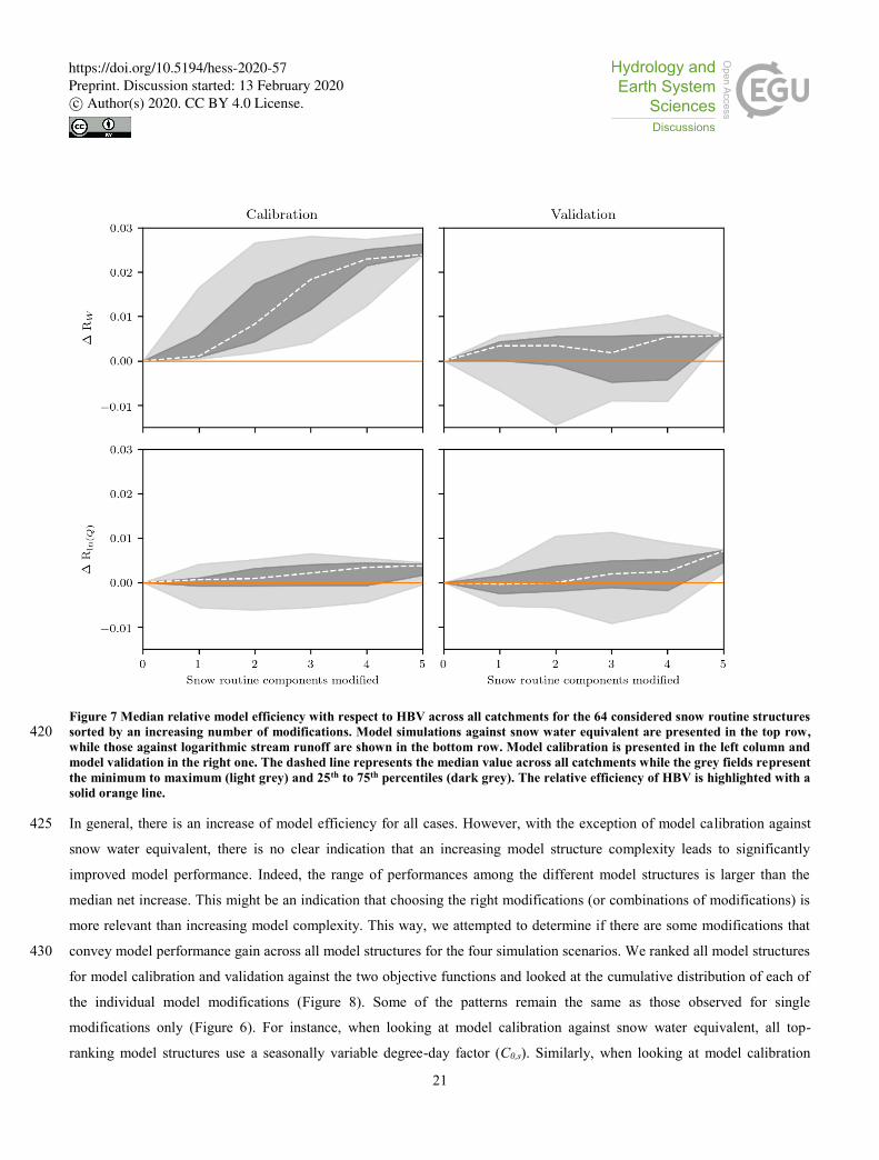
Figure 7 Median relative model efficiency with respect to HBV across all catchments for the 64 considered snow routine structures
sorted by an increasing number of modifications. Model simulations against snow water equivalent are presented in the top row, 420 while those against logarithmic stream runoff are shown in the bottom row. Model calibration is presented in the left column and
model validation in the right one. The dashed line represents the median value across all catchments while the grey fields represent
the minimum to maximum (light grey) and 25th to 75th percentiles (dark grey). The relative efficiency of HBV is highlighted with a
solid orange line.
In general, there is an increase of model efficiency for all cases. However, with the exception of model calibration against 425
snow water equivalent, there is no clear indication that an increasing model structure complexity leads to significantly
improved model performance. Indeed, the range of performances among the different model structures is larger than the
median net increase. This might be an indication that choosing the right modifications (or combinations of modifications) is
more relevant than increasing model complexity. This way, we attempted to determine if there are some modifications that
convey model performance gain across all model structures for the four simulation scenarios. We ranked all model structures 430
for model calibration and validation against the two objective functions and looked at the cumulative distribution of each of
the individual model modifications (Figure 8). Some of the patterns remain the same as those observed for single
modifications only (Figure 6). For instance, when looking at model calibration against snow water equivalent, all top-
ranking model structures use a seasonally variable degree-day factor (C0,s). Similarly, when looking at model calibration
https://doi.org/10.5194/hess-2020-57Preprint. Discussion started: 13 February 2020c© Author(s) 2020. CC BY 4.0 License.

22
against stream runoff, all bottom-ranking model structures use an exponential function for precipitation phase partition (ΔPe). 435
Other patterns that could not be clearly observed when only looking at single modifications emerge here as well. Indeed,
even if a seasonal degree-day factor performs above average for most cases, this particular modification is included in all
bottom-ranking model structures for model validation against snow water equivalent. Also, structures including an
exponential function for snowmelt (Me) perform above average for all cases, even in almost all the top-ranking ones.
440
Figure 8 Cummulative plots for each of the 7 individual modifications to the snow routine of the HBV model as a function of the
ranked 64 model structures arising from all the possible combinations of modifications. The modifications are a seasonally-
variable temperature lapse rate (Γs), a linear, sinusoidal, and exponential function for the precipitation phase partition (ΔPl, ΔPs,
and ΔPe respectively), different thresholds for precipitation phase and snowmelt (TP,M), a seasonally variable degree-day factor
(C0,s), and an exponential snowmelt with no refreezing (Me). Model simulations against snow water equivalent are presented in the 445 top row, while those against logarithmic stream runoff are presented in the bottom row. Model calibration is presented in the lleft
column and model validation in the right one. Model modifications plotting above the 1:1 line (gray dotted line) tend to be
included in high-ranking model structures, while those plotting below the 1:1 line tend to be included in low ranking structures.
Indeed, looking at the ranked alternative model structures and the modifications contained in each of them, some model
modifications have proven to be dominant, even when combined with a number of other modifications. Nevertheless, these 450
dominant modifications impact the model structure performance in different ways, depending on the modelling scenario.
https://doi.org/10.5194/hess-2020-57Preprint. Discussion started: 13 February 2020c© Author(s) 2020. CC BY 4.0 License.

23
Ideally, the modifications we are considering to the HBV model should convey an improved representation of snow water
equivalent but also have a positive impact on stream runoff, both for model calibration and validation.
To achieve an improved representation of both snow water equivalent and stream runoff we should only consider model
alternatives that have a positive impact for each of the four modelling scenarios (i.e. calibration and validation efforts against 455
both objective functions). This way, we selected and ranked all model alternatives that have positive median relative
efficiency values with respect to HBV and examine which modifications are dominant (Figure 9). All of the selected
alternative model structures contain an exponential function for snowmelt (Me), and none of them includes an exponential
function for precipitation phase partition (ΔPe). Most model structures are the result of the combination of three or four
different modifications (seven alternatives each). Four alternatives contain two model modifications and two alternatives 460
include five modifications. Perhaps most interesting, two of the model alternatives only include a single modification: an
exponential snowmelt function, and a sine function for precipitation phase partition (ΔPs). Nevertheless, these alternatives
have the lowest ranking among the selection. Overall, the top-ranking alternatives contain a seasonally varying degree-day
factor (C0,s) and an exponential snowmelt function, while other modifications resulted in more variable performances.
465
Figure 9 Ranked alternative structures to the snow routine of HBV that present positive relative efficiency values with respect to
HBV for model calibration and validation against snow water equivalent and stream runoff disaggregated by snow routine
component variants. The alternatives for each of the considered model components are a linear and a seasonally-variable degree-
day factor (Γc and Γs respectively); an abrupt, linear, sinusoidal, and exponential precipitation phase partition (ΔPa, ΔPl, ΔPs, and
ΔPe respectively); a common and individualised threshold temperature for precipitation phase partition and snowmelt (TT and 470 TP,M respectively); a constant and seasonally-variable degree-day factor (C0,c and C0,s respectively); and a linear and exponential
(with no refreezing) melt function (Ml and Me respectively). Every row contains one model structure with the selected variant for
each of the components highlighted in blue. The median relative efficiency for all modelling scenarios is given on the left y-axis
while the number of model modifications in each alternative is provided in the right y-axis.
https://doi.org/10.5194/hess-2020-57Preprint. Discussion started: 13 February 2020c© Author(s) 2020. CC BY 4.0 License.
24
4 Discussion 475
From the results obtained in this study we can conclude that it is difficult to improve existing hydrological models and
especially those that, like HBV, have proven capable of reproducing the hydrological behaviour of catchments over an
extensive range of environmental and geographical conditions (Bergström, 2006). That being said, some of the proposed
modifications to the snow routine of the HBV model that we tested in this study showed a generally positive impact on the
model performance for simulating both snow water equivalent and stream runoff, albeit to different extents. The most 480
valuable single model modifications for modelling mountainous catchments in Central Europe are the use of an exponential
snowmelt function and, to a lesser extent, a seasonally-varying degree-day factor. Another modification, using different
thresholds for snowfall and snowmelt instead of a single threshold, produces significant improvements towards snow water
equivalent, but does not convey any advantage for simulating stream runoff.
Continuing on the impact of model modifications on the different objective functions we considered in this study, we have 485
seen that there are large differences between them. In general, the impact is more evident when simulating snow water
equivalent, as the simulated stream runoff is modulated and smoothened out by the other routines of the model (i.e. soil,
groundwater, and routing routines), which partially compensate and mask any modifications made on the snow routine
(Clark and Vrugt, 2006). Additionally, some of the modifications that improve the performance of the model to simulate
snow water equivalent, such as the use of an exponential function to define the solid and liquid phases of precipitation, 490
clearly penalise the stream runoff simulations.
Unlike most modifications considered in this study, which are simplifications of complex processes, the use of an
exponential function to describe precipitation phase partition and the use of a seasonally varying temperature lapse rate are
both modifications derived from empirical evidence (Magnusson et al., 2014; Rolland, 2002). Nevertheless, as we have
previously discussed, neither of these modifications translate into an improvement of model performance for any of the 495
objective functions. This might be due to the fact that, since the models are based on simplifications and generalisations of
the processes that occur in reality, these accurate measurements of the processes do not align well with other simplifications
made in the model structure and/or behaviour or the chosen spatio-temporal resolution (Harder and Pomeroy, 2014;
Magnusson et al., 2015).
Other modifications are relatively similar to each other, such as the case of using linear and sine functions to describe 500
precipitation phase partition. Both these conceptualisations require only one additional parameter, and perform almost
identical. Indeed, precipitation partition between rain and snow is exactly the same for both conceptualisations for most of
the transition temperature range. The only divergence is in the tails, which are abrupt for the linear case and smooth for the
sine one. Provided that the smooth transition is a more accurate description of the physical process which, in addition, avoids
the introduction of discontinuities into the objectives functions, which might complicate model calibration (Kavetski and 505
Kuczera, 2007), and that both modifications include the same degree of complexity and perform nearly identical, we should
https://doi.org/10.5194/hess-2020-57Preprint. Discussion started: 13 February 2020c© Author(s) 2020. CC BY 4.0 License.

25
favour the most accurate description. Nevertheless, some models, including HBV, continue to use the linear
conceptualisation with the argument of simplicity.
We observe differences in model performance among the two geographical domains included in this study. Most notably, the
modifications on precipitation phase partition penalised the model performance on most Czech catchments for simulating 510
snow water equivalent, while having the opposite impact for Swiss catchments. The Czech catchments have a narrower
elevation range compared to the Swiss catchments, in addition to an earlier and shorter snowmelt period. These
characteristics may favour the simplification of an abrupt transition between rain and snow, while using gradual transitions
between rain and snow favours the more extended melt season and larger elevation ranges of the Swiss catchments. Another
factor that may impact the results is the significant differences in model driving and validation data availability for each of 515
the geographical domains (Günther et al., 2019; Meeks et al., 2017). Indeed, while in Czechia there are a limited number of
meteorological stations providing temperature, precipitation and snow water equivalent data, the Swiss catchments benefit
from distributed data for the different catchment elevations, allowing for more accurate calibration of snow-related
parameters.
Nevertheless, even with the large differences in hydrological regime, catchment morphology, and data availability between 520
the two geographical domains, the impact of the different modifications to model performance was in general comparable
among them. This is a relevant point because HBV aims to be a general-purpose hydrological model that is applicable to a
range of geographical domains and both in areas with data wealth and scarcity. Achieving comparable model performances
under these different conditions is an indication of the suitability and strength of the HBV model for such goals.
Regarding model complexity and uncertainty, we found that increasing the complexity, and thus the number of parameters of 525
the model, generally translated into a broader range of model performances, indicating that the uncertainty related to the
model structure was also increased. This is a well-known problem of hydrological models, and the focus of many studies
(Essery et al., 2013; Strasser et al., 2002). Additionally, we found that, for most cases, the median model performance
increase with increasing model complexity was not significant with respect to the performance range. This means that an
increasing model complexity does not necessarily translate into better model performance, which is consistent with other 530
studies (Orth et al., 2015). This fact highlights the importance of carefully choosing the degree of complexity of the model
based on the objectives to be achieved and the available data (Hock, 2003; Magnusson et al., 2015).
Even if model complexity is not desirable by itself if implemented in a sensible way, it can improve the performance of
hydrological models. Indeed, 22 of the 63 model structure alternatives that we tested in this study (all of them conveying an
increase of model complexity) convey and increase in model performance with respect to HBV for all cases. Furthermore, 535
out of these 22 alternatives, only two of them consist of a single modification, while most have 3 or 4 modifications.
Nevertheless, all of these alternatives share common traits such as using an exponential snowmelt function with no
refreezing. Indeed, almost all model structures that do not have this particular modification perform worse than HBV in at
least one simulation scenario.
https://doi.org/10.5194/hess-2020-57Preprint. Discussion started: 13 February 2020c© Author(s) 2020. CC BY 4.0 License.

26
Considering these results, it is reasonable to state that, while the increased realism arising from the interplay among the 540
different modifications in these model structure alternatives play a role in improving the model performance, this is mainly
the result of a few dominant modifications. This way, the use of an exponential snowmelt function is the most valuable
single modification with a median performance increase of 0.002 with respect to HBV for all simulations (with individual
performance increases over 0.1). However, when we combine it with a seasonal degree-day factor, we achieve a median
performance increase of 0.008, almost the highest performance increase amongst all model alternatives. Adding further 545
complexity to the model does not convey significant improvements with respect to this model structure. Consequently, if we
were to implement any modifications to the model, they would be to substitute the linear snowmelt and refreezing
conceptualisation by an exponential snowmelt function, and replacing the constant degree-day factor by a seasonally varying
one, in that order.
Finally, it is important to mention that these results are only valid for the selected study areas and cannot be extrapolated to 550
all the different alpine and snow-covered areas around the world. The different processes involved in different settings are
likely to favour different conceptualisations of the snow processes. So, while the proposed modifications might be useful to
tailor the model to Central-European alpine catchments, we still consider the default model structure of HBV as a very
capable general purpose model that can be used in a variety of settings and for different purposes.
5 Conclusions 555
We evaluated the performance of the snow routine of the HBV model and explored possible modifications to make it more
realistic and relevant for hydrological modelling in Alpine areas in Central Europe. We tested a number of modifications to
all of the different components of the snow routine over a large number of catchments covering a range of geographical
settings, and different data availability conditions on their ability to reproduce both snow water equivalent and stream runoff.
We found that the results differ greatly across the different catchments, objective functions, and simulation type 560
(calibration/validation). However, the results allow drawing the following general conclusions regarding the value of the
different model modifications for the performance in mountainous catchments in Central Europe:
The comparatively simple default structure of the HBV model performs well when simulating snow-related
processes and their impact to stream runoff in most of the examined catchments.
An increased model complexity does not by itself add any value to the ability of the model to reproduce snow water 565
equivalent and stream runoff. A careful examination of the design choices of the model for the given application,
data availability and objective is a significantly better approach.
An exponential snowmelt function with no refreezing is the single most valuable overall modification to the snow
routine structure, followed by a seasonally variable degree-day factor. Adding further complexity to the model does
not necessarily translate in significant performance improvements. 570
https://doi.org/10.5194/hess-2020-57Preprint. Discussion started: 13 February 2020c© Author(s) 2020. CC BY 4.0 License.

27
These results are not transferrable to other geographical domains or purposes, but the methodology presented here may be
used to assess the suitability of model design choices.
6 Data availability
Meteorological and hydrological data to calibrate the HBV model were obtained from the Swiss Federal Office of
Meteorology and Climatology, the Swiss Federal Office for the Environment, and the Czech Hydrometeorological Institute. 575
The HBV model outputs are available from the first author upon request.
7 Author contribution
JS initiated the study. MGL developed the methodology and performed all analyses. MGL, NG, and MJ prepared the input
meteorological and hydrological data used to calibrate the HBV model. MJPV performed all the necessary modifications to
the source code of the HBV model. MGL prepared the manuscript with contributions from all co-authors. 580
8 Competing interests
The authors declare that they have no conflict of interest.
9 Acknowledgements
This project was partially funded by the Swiss Federal Office for the Environment (FOEN). The contribution of Michal
Jenicek was supported by the Czech Science Foundation, project no. GA18-06217Y. 585
References
Avanzi, F., De Michele, C., Morin, S., Carmagnola, C. M., Ghezzi, A. and Lejeune, Y.: Model complexity and data
requirements in snow hydrology: seeking a balance in practical applications, Hydrol. Process., 30(13), 2106–2118,
doi:10.1002/hyp.10782, 2016.
Barnett, T. P., Adam, J. C. and Lettenmaier, D. P.: Potential impacts of a warming climate on water availability in snow-590
dominated regions, Nature, 438(7066), 303–309, doi:10.1038/nature04141, 2005.
Berghuijs, W. R., Woods, R. A. and Hrachowitz, M.: A precipitation shift from snow towards rain leads to a decrease in
streamflow-supplement, Nat. Clim. Chang., 4(7), 583–586, doi:10.1038/NCLIMATE2246, 2014.
Bergström, S.: The HBV Model, in Computer Models of Watershed Hydrology, edited by V. P. Singh, pp. 443–476, Water
Resources Publications, Highlands Ranch, CO., 1995. 595
https://doi.org/10.5194/hess-2020-57Preprint. Discussion started: 13 February 2020c© Author(s) 2020. CC BY 4.0 License.

28
Bergström, S.: Experience from applications of the HBV hydrological model from the perspective of prediction in ungauged
basins, IAHS Publ., 307, 97–107, 2006.
Braun, J. N. and Renner, C. B.: Application of a conceptual runoff model in different physiographic regions of Switzerland,
Hydrol. Sci. J., 37(3), 217–231, doi:10.1080/02626669209492583, 1992.
Clark, M. P. and Vrugt, J. A.: Unraveling uncertainties in hydrologic model calibration: Addressing the problem of 600
compensatory parameters, Geophys. Res. Lett., 33(6), 1–5, doi:10.1029/2005GL025604, 2006.
Collins, E. H.: Relationship of Degree-Days above Freezing to Runoff, Eos, Trans. Am. Geophys. Union, 15(2), 624–629,
1934.
Dai, A.: Temperature and pressure dependence of the rain-snow phase transition over land and ocean, Geophys. Res. Lett.,
35(12), 1–7, doi:10.1029/2008GL033295, 2008. 605
Debele, B., Srinivasan, R. and Gosain, A. K.: Comparison of process-based and temperature-index snowmelt modeling in
SWAT, Water Resour. Manag., 24(6), 1065–1088, doi:10.1007/s11269-009-9486-2, 2010.
Essery, R., Morin, S., Lejeune, Y. and Ménard, C. B.: A comparison of 1701 snow models using observations from an alpine
site, Adv. Water Resour., 55, 131–148, doi:10.1016/j.advwatres.2012.07.013, 2013.
Fang, S., Xu, L., Pei, H., Liu, Y., Liu, Z., Zhu, Y., Yan, J. and Zhang, H.: An Integrated Approach to Snowmelt Flood 610
Forecasting in Water Resource Management, IEEE Trans. Ind. Informatics, 10(1), 548–558, doi:10.1109/TII.2013.2257807,
2014.
Flügel, W.-A.: Hydrological response units (HRUs) to preserve basin heterogeneity in hydrological modelling using
PRMS/MMS - case study in the Bröl basin, Germany, in Modelling and Management of Sustainable Basin-scale Water
Resource Systems, vol. 231, pp. 79–87, International Association of Hydrological Sciences (IAHS), Boulder, CO., 1995. 615
FOEN: Observed Discharge Time Series of Swiss Rivers, 2017.
Frei, C.: Interpolation of temperature in a mountainous region using nonlinear profiles and non-Euclidean distances, Int. J.
Climatol., 34, 1585–1605, doi:10.1002/joc.3786, 2014.
Frei, C. and Schär, C.: A precipitation climatology of the Alps from high-resolution rain-gauge observations, Int. J.
Climatol., 18, 873–900, doi:10.1002/(SICI)1097-0088(19980630)18:8<873::AID-JOC255>3.0.CO;2-9, 1998. 620
Frei, C., Schöll, R., Fukutome, S., Schmidli, J. and Vidale, P. L.: Future change of precipitation extremes in Europe:
Intercomparison of scenarios from regional climate models, J. Geophys. Res., 111, doi:10.1029/2005JD005965, 2006.
Freudiger, D., Kohn, I., Seibert, J., Stahl, K. and Weiler, M.: Snow redistribution for the hydrological modeling of alpine
catchments, Wiley Interdiscip. Rev. Water, 4(5), e1232, doi:10.1002/wat2.1232, 2017.
Frey, S. and Holzmann, H.: A conceptual, distributed snow redistribution model, Hydrol. Earth Syst. Sci., 19(11), 4517–625
4530, doi:10.5194/hess-19-4517-2015, 2015.
Froidurot, S., Zin, I., Hingray, B. and Gautheron, A.: Sensitivity of Precipitation Phase over the Swiss Alps to Different
Meteorological Variables, J. Hydrometeorol., 15(2), 685–696, doi:doi:10.1175/JHM-D-13-073.1, 2014.
Gabbi, J., Carenzo, M., Pellicciotti, F., Bauder, A. and Funk, M.: A comparison of empirical and physically based glacier
https://doi.org/10.5194/hess-2020-57Preprint. Discussion started: 13 February 2020c© Author(s) 2020. CC BY 4.0 License.

29
surface melt models for long-term simulations of glacier response, J. Glaciol., 60(224), 1199–1207, 630
doi:10.3189/2014JoG14J011, 2014.
Griessinger, N., Seibert, J., Magnusson, J. and Jonas, T.: Assessing the benefit of snow data assimilation for runoff modeling
in Alpine catchments, Hydrol. Earth Syst. Sci., 20(9), 3895–3905, doi:10.5194/hess-20-3895-2016, 2016.
Günther, D., Marke, T., Essery, R. and Strasser, U.: Uncertainties in Snowpack Simulations—Assessing the Impact of Model
Structure, Parameter Choice, and Forcing Data Error on Point-Scale Energy Balance Snow Model Performance, Water 635
Resour. Res., 55(4), 2779–2800, doi:10.1029/2018WR023403, 2019.
Hannah, D. M., Brown, L. E., Milner, A. M., Gurnell, A. M., McGregor, G. R., Petts, G. E., Smith, B. P. G. and Snook, D.
L.: Integrating climate-hydrology-ecology for alpine river systems, Aquat. Conserv. Mar. Freshw. Ecosyst., 17, 636–656,
doi:10.1002/aqc.800, 2007.
Harder, P. and Pomeroy, J. W.: Hydrological model uncertainty due to precipitation-phase partitioning methods, Hydrol. 640
Process., 28(14), 4311–4327, doi:10.1002/hyp.10214, 2014.
Harpold, A. A., Kaplan, M. L., Zion Klos, P., Link, T., McNamara, J. P., Rajagopal, S., Schumer, R. and Steele, C. M.: Rain
or snow: Hydrologic processes, observations, prediction, and research needs, Hydrol. Earth Syst. Sci., 21(1), 1–22,
doi:10.5194/hess-21-1-2017, 2017.
Hock, R.: A distributed temperature-index ice- and snowmelt model including potential direct solar radiation, J. Glaciol., 645
45(149), 101–111, doi:10.1017/S0022143000003087, 1999.
Hock, R.: Temperature index melt modelling in mountain areas, J. Hydrol., 282(1–4), 104–115, doi:10.1016/S0022-
1694(03)00257-9, 2003.
Hock, R.: Glacier melt: a review of processes and their modelling, Prog. Phys. Geogr., 29(3), 362–391,
doi:10.1191/0309133305pp453ra, 2005. 650
Hottelet, C., Blažková, Š. and Bičík, M.: Application of the ETH Snow Model to Three Basins of Different Character in
Central Europe, Nord. Hydrol., 25(1–2), 113–128, 1994.
Jamieson, B. and Stethem, C.: Snow avalanche hazards and management in Canada: Challenges and progress, Nat. Hazards,
26(1), 35–53, doi:10.1023/A:1015212626232, 2002.
Jenicek, M. and Ledvinka, O.: Importance of snowmelt contribution to seasonal runoff and summer low flows in Czechia, 655
Hydrol. Earth Syst. Sci. Discuss., doi:10.5194/hess-2019-611, 2020.
Kane, D. L., Gieck, R. E. and Hinzman, L. D.: Snowmelt Modeling at Small Alaskan Arctic Watershed, J. Hydrol. Eng.,
2(4), 204–210, doi:10.1061/(ASCE)1084-0699(1997)2:4(204), 1997.
Kavetski, D. and Kuczera, G.: Model smoothing strategies to remove microscale discontinuities and spurious secondary
optima im objective functions in hydrological calibration, Water Resour. Res., 43(3), 1–9, doi:10.1029/2006WR005195, 660
2007.
Lindström, G., Johansson, B., Persson, M., Gardelin, M. and Bergström, S.: Development and test of the distributed HBV-96
hydrological model, J. Hydrol., 201, 272–288, doi:10.1016/S0022-1694(97)00041-3, 1997.
https://doi.org/10.5194/hess-2020-57Preprint. Discussion started: 13 February 2020c© Author(s) 2020. CC BY 4.0 License.

30
Magnusson, J., Gustafsson, D., Hüsler, F. and Jonas, T.: Assimilation of point SWE data into a distributed snow cover model
comparing two contrasting methods, Water Resour. Res., 50, 7816–7835, doi:10.1002/ 2014WR015302, 2014. 665
Magnusson, J., Wever, N., Essery, R., Helbig, N., Winstral, A. and Jonas, T.: Evaluating snow models with varying process
representations for hydrological applications, Water Resour. Res., 51(4), 2707–2723, doi:10.1002/2014WR016498, 2015.
Martinec, J.: The degree–day factor for snowmelt runoff forecasting, in IUGG General Assembly of Helsinki, vol. 51, pp.
468–477, IAHS Commission of Surface Waters, Helsinki, Finland., 1960.
Meeks, J., Moeck, C., Brunner, P. and Hunkeler, D.: Infiltration under snow cover: Modeling approaches and predictive 670
uncertainty, J. Hydrol., 546, 16–27, doi:10.1016/j.jhydrol.2016.12.042, 2017.
Merz, R. and Blöschl, G.: A process typology of regional floods, Water Resour. Res., 39(12), 1–20,
doi:10.1029/2002WR001952, 2003.
Nash, J. E. and Sutcliffe, J. V.: River flow forecasting through conceptual models part I: A discussion of principles, J.
Hydrol., 10, 282–290, doi:10.1016/0022-1694(70)90255-6, 1970. 675
Ohmura, A.: Physical Basis for the Temperature-Based Melt-Index Method, J. Appl. Meteorol., 40(4), 753–761,
doi:10.1175/1520-0450(2001)040<0753:PBFTTB>2.0.CO;2, 2001.
Orth, R., Staudinger, M., Seneviratne, S. I., Seibert, J. and Zappa, M.: Does model performance improve with complexity? A
case study with three hydrological models, J. Hydrol., 523, 147–159, doi:10.1016/j.jhydrol.2015.01.044, 2015.
Pellicciotti, F., Brock, B., Strasser, U., Burlando, P., Funk, M. and Corripio, J.: An enhanced temperature-index glacier melt 680
model including the shortwave radiation balance: development and testing for Haut Glacier d’Arolla, Switzerland, J.
Glaciol., 51, doi:10.3189/172756505781829124, 2005.
Riboust, P., Thirel, G., Moine, N. Le and Ribstein, P.: Revisiting a simple degree-day model for integrating satellite data:
implementation of swe-sca hystereses, J. Hydrol. Hydromechanics, 67(1), 70–81, doi:10.2478/johh-2018-0004, 2019.
Rico, M., Benito, G., Salgueiro, A. R., Díez-Herrero, A. and Pereira, H. G.: Reported tailings dam failures. A review of the 685
European incidents in the worldwide context, J. Hazard. Mater., 152(2), 846–852, doi:10.1016/j.jhazmat.2007.07.050, 2008.
Rolland, C.: Spatial and Seasonal Variations of Air Temperature Lapse Rates in Alpine Regions, J. Clim., 16, 1032–1046,
doi:10.1175/1520-0442(2003)016<1032:SASVOA>2.0.CO;2, 2002.
Schaefli, B. and Gupta, H. V.: Do Nash values have value?, Hydrol. Process., 21, 2075–2080, doi:10.1002/hyp.6825, 2007.
Schweizer, J., Jamieson, J. B. and Schneebeli, M.: Snow avalanche formation, Rev. Geophys., 41(4), 690
doi:10.1029/2002RG000123, 2003.
Seibert, J.: Regionalisation of parameters for a conceptual rainfall-runoff model, Agric. For. Meteorol., 98–99, 279–293,
doi:10.1016/S0168-1923(99)00105-7, 1999.
Seibert, J.: Multi-criteria calibration of a conceptual runoff model using a genetic algorithm, Hydrol. Earth Syst. Sci., 4(5),
215–224, 2000. 695
Seibert, J. and Vis, M. J. P.: Teaching hydrological modeling with a user-friendly catchment-runoff-model software package,
Hydrol. Earth Syst. Sci., 16, 3315–3325, doi:10.5194/hess-16-3315-2012, 2012.
https://doi.org/10.5194/hess-2020-57Preprint. Discussion started: 13 February 2020c© Author(s) 2020. CC BY 4.0 License.

31
Sims, E. M. and Liu, G.: A Parameterization of the Probability of Snow–Rain Transition, J. Hydrometeorol., 16(4), 1466–
1477, doi:10.1175/JHM-D-14-0211.1, 2015.
Strasser, U., Etchevers, P. and Lejeune, Y.: Inter-comparison of two snow models with different complexity using data from 700
an alpine site, Nord. Hydrol., 33(1), 15–26, doi:10.2166/nh.2002.0002, 2002.
Sui, J. and Koehler, G.: Rain-on-snow induced flood events in southern Germany, J. Hydrol., 252(1–4), 205–220,
doi:10.1016/S0022-1694(01)00460-7, 2001.
Valéry, A., Andréassian, V. and Perrin, C.: “As simple as possible but not simpler”: What is useful in a temperature-based
snow-accounting routine? Part 1 - Comparison of six snow accounting routines on 380 catchments, J. Hydrol., 517, 1166–705
1175, doi:10.1016/j.jhydrol.2014.04.059, 2014.
Verdhen, A., Chahar, B. R. and Sharma, O. P.: Snowmelt modelling approaches in watershed models: Computation and
comparison of efficiencies under varying climatic conditions, Water Resour. Manag., 28(11), 3439–3453,
doi:10.1007/s11269-014-0662-7, 2014.
Vis, M., Knight, R., Pool, S., Wolfe, W. and Seibert, J.: Model calibration criteria for estimating ecological flow 710
characteristics, Water, 7(5), 2358–2381, doi:10.3390/w7052358, 2015.
Viviroli, D., Gurtz, J. and Zappa, M.: The hydrological modelling system PREVAH, edited by S. Steiner, Geographica
Bernensia P40, Berne, Switzerland., 2007.
Walter, M. T., Brooks, E. S., McCool, D. K., King, L. G., Molnau, M. and Boll, J.: Process-based snowmelt modeling: does
it require more input data than temperature-index modeling?, J. Hydrol., 300(1–4), 65–75, 715
doi:10.1016/j.jhydrol.2004.05.002, 2005.
Watson, B. M. and Putz, G.: Comparison of Temperature-Index Snowmelt Models for Use within an Operational Water
Quality Model, J. Environ. Qual., 43(1), 199–207, doi:10.2134/jeq2011.0369, 2014.
Weingartner, R. and Aschwanden, H.: Discharge Regime - the Basis for the Estimation of Average Flows, Plate 5.2, in
Hydrological Atlas of Switzerland, edited by R. Weingartner and S. M., Swiss Federal Office for Water and Geology, Bern, 720
Switzerland., 1989.
Wever, N., Fierz, C., Mitterer, C., Hirashima, H. and Lehning, M.: Solving Richards Equation for snow improves snowpack
meltwater runoff estimations in detailed multi-layer snowpack model, Cryosphere, 8(1), 257–274, doi:10.5194/tc-8-257-
2014, 2014.
725
https://doi.org/10.5194/hess-2020-57Preprint. Discussion started: 13 February 2020c© Author(s) 2020. CC BY 4.0 License.


![A Quantitative Physical Model of the Snow Crystal ...morphology of snow crystals growing in air as a function of temperature and water vapor supersaturation (from [1990Yok]). 2 especially](https://static.fdocuments.in/doc/165x107/5ed7caaba904e157fb28c3df/a-quantitative-physical-model-of-the-snow-crystal-morphology-of-snow-crystals.jpg)