Complexity and Flexibility in Call Center Scheduling Models

International Journal of Business and Social Science Volume 8 • Number 12 • December 2017

1

Complexity and Flexibility in Call Center Scheduling Models

Thomas R. Robbins

East Carolina University

College of Business

Department of Marketing and Supply Chain

3136 Bate Building

Greenville, NC 27858-4353

Abstract

Call center scheduling models have historically presented a significant challenge to operations researchers and

practitioners alike. Though conceptually simple to describe, the models can quickly become quite complex and

computationally intensive. Increasing the flexibility of the scheduling model, for example by adding additional

scheduling options lowers cost but can drive the model to a size that is impractical or impossible to solve to

optimality. In this paper we examine the trade-off between flexibility and complexity. We investigate the

feasibility of solving these models in what is often the call center supervisor’s tool of choice – Excel. We present

two different formulations with a number of scheduling options for each. We discuss strategies to achieve

practical solution time frames using the Excel-based Risk Solver Platform engine. Our analysis shows that more

sophisticated models provide improved schedules and that Excel is a viable modeling platform for this problem.

Keywords: Service Operations, Scheduling, Flexibility

1 Introduction

Call center scheduling models have historically presented a significant challenge to operations researchers and

practitioners alike. Though conceptually simple to describe, the models can quickly become quite complex and

computationally intensive. In a standard model call center management forecasts the number of calls expected to

arrive in each of a pre-defined number of discrete time periods, often every half hour. Period by period staffing

requirements are then determined based on some service level objective. For example, staff enough agents so that

in each time period a minimum of 80% of the calls are answered within 30 seconds. This calculation is easily

performed using some queuing model such as the Erlang-C model, or the more sophisticated Erlang-A model.

Based on the call center’s hours of operation and its staffing policy a menu of possible shifts is defined. The

scheduling objective is then to find the lowest cost combination of shift assignments that meets the staffing

requirement. This model is easily formulated as an integer program in what is known as a set-covering model.

The model has one decision variable for each possible shift and one constraint for each time period. A basic

model formulation was presented and solved by Dantzig as early as 1954. The model expressed in that paper is

trivially easy to solve using current technology.

The model however does not scale well, and once a few assumptions are relaxed, the set covering model becomes

NP-Complete. Straightforward scheduling options, such as 24-hour operation, explicitly scheduled breaks, or part

time shifts, create a combinatorial explosion that can quickly drive the model to a size that is impractical or

impossible to solve to optimality. In the years since Dantzig’s paper was first published a number of researchers

have analyzed the problem and put forward approaches to solve large-scale problems. New formulations have

also been developed that address some of the key functional limitations in the basic set covering approach, for

example the desire to achieve a service level goal over an entire day instead of in each 30-minute period. These

formulations further increased the size and complexity of the scheduling problem.

In this paper we examine the call center-scheduling problem. We examine the impact flexibility has on

complexity and cost. Our primary objective is to examine the benefits of scheduling flexibility and its

relationship to computational complexity. We seek to show that increased flexibility, in the form of more

scheduling options yields lower cost solutions. Secondly, we seek to show that although computational

complexity increases significantly that these models can be solved even on desktop platforms.

ISSN 2219-1933 (Print), 2219-6021 (Online) © Center for Promoting Ideas, USA www.ijbssnet.com

2

We present two different formulations of the call center scheduling problem and analyze the scale of the model

within those formulations based on business policy decisions. We discuss strategies to achieve practical solution

time frames using the Excel-based Risk Solver Platform (RSP) engine and evaluate the potential improvements

that can be gained from using more sophisticated models.

The remainder of this paper is organized as follows. Section 2 provides a summary of the relevant literature.

Section 3 presents several variations of the set-covering model. We solve and compare multiple instances of the

model, comparing relative costs and solution times. Section 4 presents a second formulation that implements a

global service level requirement. Section 5 provides a summary and outlines future research topics.

2 Related Literature

2.1 Call Center Scheduling Literature

There is a very substantial body of literature addressing call center issues. A comprehensive review of the

literature, including papers that address the scheduling problem can be found in Gans, Koole, & Mandelbaum

(2003). Robbins(2010) provides an overview of the range of scheduling models applicable to call centers.

A basic model for shift scheduling is presented in Dantzig (1954). This paper examines scheduling in the context

of a toll booth problem, but the basic set-covering model presented is directly applicable to call center scheduling.

In the set covering approach call center scheduling is inherently a two-stage process. In the first stage a queuing

model is used to determine period by period staffing levels. So, for example, the staffing requirement in each

period might be set to the level required to achieve a targeted minimum level of surface. That level is calculated

based on a queuing model, typically the Erlang C or Erlang A model (Gans et al., 2003). Staffing levels are

determined exogenously to the set covering model, providing a period by period staffing level that must be

satisfied. The set-covering model problem is known to be NP Complete unless it possesses the cyclic 1’s property

(Garey and Johnson 1979); that is unless each shift is continuous with no breaks. NP Completeness implies the

lack of a polynomial time solution algorithm. Practically this means staff scheduling problems that include

explicit breaks, whether those are breaks for lunch or breaks between days, are inherently unscalable. Much of the

research related to staff scheduling is related either directly or indirectly, to this scalability problem.

Researchers have addressed this problem in several ways; through problem simplification, heuristic methods, and

alternative algorithms. Henderson & Berry (1976) applied two types of heuristics. The first heuristic reduces the

number of shift types, scheduling against only a reduced set of schedules referred to as the working subset. The

working set was selected either using a most different selection algorithm, or by randomly sampling from the set

of possible schedules. Their analysis showed good results for random sampling when a reasonably large number

of schedules are used.

An alternate stream of research attacks the problem using an implicit scheduling approach. Implicit scheduling

models generally use a two-phased approach, generating an overall schedule in the first phase, and then placing

breaks in the second phase. Implicit scheduling approaches are addressed in Bechtold & Jacobs (1990),

Thompson (1995) and Aykin (1996). Thompson (1995) includes a summary of related papers and then develops

a Doubly-Implicit Shift Scheduling Model (DISSM). Aykin (1996) addresses problems with multiple break

windows. Several other papers address related problems (Brusco & Jacobs, 1998, 2000; Brusco & Johns, 1996).

An alternative to the two-staged approach is to integrate the staffing requirement and shift scheduling steps into a

single joint staffing and scheduling model. Many models of this type use simulation based optimization, but the

concept can be applied in discrete optimization as well. Robbins & Harrison(2010) use a piecewise linear

approximation of the service level curve to perform a joint staffing and scheduling model. A key advantage of the

joint approach is that the model can implement a global service level requirement instead of, or in addition to, the

period by period service level requirement inherent in the two-stage approach. In call centers with short interval

peaks staffing to satisfy the peak arrival rate may result in excess capacity in other periods. In response to this

issue some call centers seek to achieve their service level targets over an extended period; perhaps a day, week or

even a month. This is often referred to as a global service constraint.

Excel is a ubiquitous tool in the business world. Practitioners use Excel for a wide range of data analysis and

reporting functions. Excel is also used as an optimization platform that is extremely popular in undergraduate and

graduate business education. Popular textbooks such as Ragsdale (2017) teach the concepts of optimization using

Excel and optimization add-ins such as Solver and Risk Solver Platform.

http://www.ijbssnet.com/


3

The use of Excel as a commercial tool for Operations Research applications in general, and optimization in

particular, is becoming increasingly popular. LeBlanc & Galbreth (2007) describes a supply chain optimization

model implemented with Excel and Visual Basic for Applications (VBA). A special edition of the applied OR

journal Interfaces is devoted to the use of spreadsheets in OR applications. LeBlanc & Grossman (2008) provide

an overview. Several papers in this issue specifically involve optimization models. Gurgur & Morley (2008)

describe a chance constrained optimization model for selecting infrastructure projects. Kumiega & Van Vliet

(2008) present a financial portfolio optimization application. Ovchinnikov & Milner (2008) discuss an application

for assigning medical school residents to job rotations. Pasupathy & Medina-Borja (2008) present an application

that supports resource allocation decision for the American Red Cross.

Other papers and other journals have also presented Excel based optimization models. Grover & Lavin (2007)

also develop a portfolio optimization model using Excel and Solver. Grossman & Özlük (2009) develop an

enhanced scenario management tool with Excel and Solver. Multiple papers are focused on how specific problem

types can be solved in Excel. The assignment problem is addressed in M. Patterson & Harmel (2001),

transportation problems in M. Patterson & Harmel, (2002), and the Traveling Salesman problem in M. C.

Patterson & Harmel (2003). Perzina & Ramík (2014) examine using Excel to solve Multicriteria decision

problems and Sil, Banerjee, Kumar, Bui, & Saikia (2013) use Excel to optimize the design of a pipe network.

3 A Set-Covering Formulation

Model one is our simplest model. It is a basic set covering model where the staffing level figures are defined

exogenously. The standard approach is to forecast call volumes in each period. A queuing model, most

commonly the Erlang C or Erlang A model, is then used to determine the number of agents required to achieve a

target staff level in each individual time-period. The optimization problem is to pick the set of schedules that

covers the requirement as efficiently as possible. Mathematically the model can be expressed as

Minimize j j

j J

c x

(1)

Subject to

ij j i

j J

a x b I

(2)

jx (3)

Where J is the set of schedules and I is the set of time periods. The integer decision variable jx represents the

number of workers assigned to the schedule j. Each assignment has a cost of jc . The objective function (1)

minimizes the weighted cost of staffing. Parameterija is a binary indicator that defines which schedules cover

which periods and parameter ib defines the per-period staffing requirement. Constraint (2) requires that the

minimum staffing requirement is satisfied in every time-period. Constraint (3) requires that schedule assignments

are non-negative integers.

The complexity of this problem is driven by the number of schedules and to a lesser extent the number of time

periods. The model includes one constraint for each time-period and one decision variable for each schedule

option. The number of schedules is the primary driver of computational complexity. A detailed model that

schedules to the half hour time-period for a week will have 336 constraints. This same model can have many

thousand schedules to choose from depending on the flexibility of staffing and the scheduling of agent breaks. It

is worth noting that nothing in Model 1 is unique to the call center environment. The model can be used in any

scenario where we have an externally defined staffing requirement and a number of scheduling options to select

from. It was in fact first presented by Dantzig in the context of toll booth operators.

In the remainder of this section we will analyze several instances of this model. We start with a simple problem

of scheduling a single day of operations with full time shifts. We progress to a week-long schedule for a 24x7

operation with explicit breaks and flexible scheduling options. Along the way our model grows from trivial to

quite complex.


4

3.1 Instance 1 – Simple Day Schedule

In this instance we examine a simple model that schedules a call center that is open less than 24 hours. Only full-

time shifts are scheduled, and breaks are not explicitly scheduled. Staffing requirements are specified in 30-

minute increments. The model has a maximum of 48 constraints and up to 31 decision variables (the exact

number depends on specific hours of operation). The model is easily solved to optimality in a fraction of a second

(typically less than .25 seconds) using the Standard LP/Quadratic engine.

Although this model is typically specified as an integer program, because of the Cyclic 1’s property the integer

constraints are not required to achieve an integral solution. Because the number of agents required are integral

and the schedules are contiguous, the optimal solution of the Linear Program relaxation will always be integer

valued.

Formulating this model in Excel is quite straightforward. The bulk of the formulation is the definition of the

schedule to matrix mapping, the aij coefficients in equation (2). A portion of the matrix is shown in

Figure 1. The cells in this matrix are configured with an auto format feature so that a 1 is shaded and a 0 is un-

shaded.

Figure 1 – Schedule Matrix

Two rows are required to establish the constraints in equation (2), a portion of which are shown in

Figure 2.

Figure 2 – Staffing constraints

While the model technically has 48 constraints, those constraints can be expressed as a single statement in RSP.

In the example $D$4:$AY$4>= $D$5:$AY$5. In addition, the decision variables are required to be non-negative.

This can be accomplished in one of two ways, adding a bound constraint ($B$11:$B$41 >= 0) or setting the non-

negative assumption on the Engine tab. Either method achieves the same result with no measurable impact on

solution time frames. The final constraint enforces integrality condition ($B$11:$B$41 = integer), though this

constraint is not actually required in this instance due to the cyclic 1’s property. Adding this constraint does not

change the result in this example, nor does it change the solution time.

The objective of this optimization problem is to minimize the cost of staffing. The cost is easily calculated by

summing up the number of agents assigned to each shift, weighted by the cost of the shift. In this example we

1 2 3 4 5 6 7 8 9 10 11 12 13 14 15 16 17 18 19

# Assigned

Name

Midnight

0:30

1:00

1:30

2:00

2:30

3:00

3:30

4:00

4:30

5:00

5:30

6:00

6:30

7:00

7:30

8:00

8:30

9:00

0 S1 1 1 1 1 1 1 1 1 1 1 1 1 1 1 1 1 1 1 0

0 S2 0 1 1 1 1 1 1 1 1 1 1 1 1 1 1 1 1 1 1

0 S3 0 0 1 1 1 1 1 1 1 1 1 1 1 1 1 1 1 1 1

0 S4 0 0 0 1 1 1 1 1 1 1 1 1 1 1 1 1 1 1 1

0 S5 0 0 0 0 1 1 1 1 1 1 1 1 1 1 1 1 1 1 1

0 S6 0 0 0 0 0 1 1 1 1 1 1 1 1 1 1 1 1 1 1

2 S7 0 0 0 0 0 0 1 1 1 1 1 1 1 1 1 1 1 1 1

3 S8 0 0 0 0 0 0 0 1 1 1 1 1 1 1 1 1 1 1 1

0 S9 0 0 0 0 0 0 0 0 1 1 1 1 1 1 1 1 1 1 1

0 S10 0 0 0 0 0 0 0 0 0 1 1 1 1 1 1 1 1 1 1

0 S11 0 0 0 0 0 0 0 0 0 0 1 1 1 1 1 1 1 1 1

0 S12 0 0 0 0 0 0 0 0 0 0 0 1 1 1 1 1 1 1 1

1 2 3 4 5 6 7 8 9 10 11 12 13 14 15 16 17 18 19

Midnight

0:30

1:00

1:30

2:00

2:30

3:00

3:30

4:00

4:30

5:00

5:30

6:00

6:30

7:00

7:30

8:00

8:30

9:00

Scheduled 0 0 0 0 0 0 2 5 5 5 5 5 7 7 9 9 11 12 13

Required 0 0 0 0 0 0 0 0 0 0 0 1 1 0 8 8 8 10 10



5

assume that the pay rate is identical for all shifts, so we minimize the number of hours. If different schedules

carried different rates, if for example late night schedules received extra compensation,

we could easily multiply the hours by the rate to obtain the total cost. In Excel the cost is easily calculated using

the Sumproduct function to multiply each shift by the hours and add the results.

(=SUMPRODUCT(B11:B41,AZ11:AZ41))

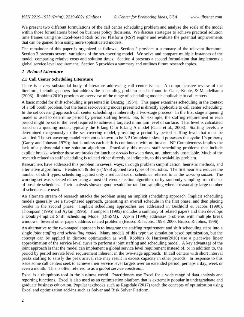
Figure 3 illustrates the staffing matrix formulated in Excel. This is a matrix of schedule mapping where a 1

indicates the schedule is on during that time period, and a 0 indicates the schedule is off during that period. The

cells in this matrix correspond to the ija parameters in equation (2). The subscript i represents the Excel column,

the subscript j represents the Excel row. The shading pattern clearly reveals the basic structure of the matrix with

9-hour shifts that start as early as midnight and end as late as 11:30.

Figure 3 – Model 1 Instance 1 in Excel

This simple base case illustrates the basic principles of many of the scheduling models we will examine. While

this initial model is almost trivial from a solution perspective, the model can grow substantially, both in its

capabilities and complexity, before we make any fundamental changes in the formulation. Figure 4 shows the

number of agents required and the number of agents scheduled for each 30-minute period.

This graph clearly illustrates one of the major problems with this scheduling problem. The constraints define the

minimum number of agents required in each period, but we are unable to achieve that minimum level in a

significant number of periods due to the scheduling options we have to choose from. One measure of the

additional cost this creates is the excess scheduling percentage, the additional hours scheduled as a percentage of

the hours required. In this example the excess scheduling percentage is 22.9%. This simple instance applies to

situations where the call center can be scheduled a day at a time and is open less than 24 hours. If either of these

conditions is not satisfied, we must move to a more complex formulation.


6

Figure 4- Scheduled and Required Staffing Levels

3.2 Instance 2 – Simple 5 Day Schedule

In this case we examine a simple model that schedules a call center that is open less than 24 hours, but requires

that we schedule employees to full time 5-day shifts. Only full-time shifts are scheduled, and breaks are not

explicitly scheduled. Staffing requirements are specified in 30-minute increments. Employees work the same

hours every day of the week. Staffing requirements however vary from day to day based on some seasonal

pattern. The advantage of scheduling for the full week is the model can best fit staffing to the full weeks demand

pattern.

This is very simple extension of instance 1. Since agents work the same hours every day the number of schedules

is unchanged at 31. However, the staffing requirement is now specified for each 30-minute period over the 5-day

work week (240 time-periods). The expanded model still has 31 decision variables, but the number of constraints

has expanded to 240. The assignment matrix now appears as in

Figure 5.

Figure 5 – Model 1 Instance 2 Schedule Matrix

Note that because of the breaks between days, this model no longer has the cyclic 1’s property and the integer

constraints are required. Other than expanding the number of columns to include all 240 time periods, and

updating the model specification to account for the extra columns the base model is essentially the same as

instance 1. From a computational perspective the time required to solve this program increases significantly, but

it is still very fast. In our testing this program solved to optimality in about 0.36 seconds.

Figure 6 shows the required and scheduled staffing level.

0

2

4

6

8

10

12

14

16

18

20

1 2 3 4 5 6 7 8 9 10 11 12 13 14 15 16 17 18 19 20 21 22 23 24 25 26 27 28 29 30 31 32 33 34 35 36 37 38 39 40 41 42 43 44 45 46 47 48

Staffing (Scheduled vs. Required)

Scheduled

Required



7

Figure 6 – Model 1 Instance 2 Staffing Profile

Matching staff levels to requirements is even more of a challenge in this model. Besides time of day seasonality,

the required staffing level also exhibits day of the week seasonality which is quite common in call centers. In this

example Monday is the busiest day and call volumes decline each day of the week. Staffing to the peak demand

on Monday morning means that the call center is overstaffed for the remainder of the week. The excess

scheduling percentage in this instance is now 36.8%

3.3 Instance 3 – 24x7 Full Time 5-day schedule

In this instance we expand the hours of operation for the call center to 7 days a week, 24 hours a day. We

continue to limit the available schedules so that agents work 5 days a week, 8 hours a day, with 2 consecutive

days off. The total number of schedules that satisfy this requirement is 336. So, in this model we now 336

integer decision variables and 240 constraints.

Figure 7 shows the assignment matrix for this model.

Figure 7 – Instance 3 Schedule Matrix

The large increase in decision variables creates a dramatic increase in solution time, but again the time is quite

reasonable. In our testing, solution time increased to about 4.7 seconds. The increased number of schedules to

choose from helps somewhat with matching supply and demand and the excess staffing percentage drops slightly

to 24.6%.

3.4 Instance 4 - 24x7 Full Time 4 and 5-day schedules

0

5

10

15

20

25

1 7 13 19 25 31 37 43 49 55 61 67 73 79 85 91 97 103

109

115

121

127

133

139

145

151

157

163

169

175

181

187

193

199

205

211

217

223

229

235

Staffing (Scheduled vs Required)

Scheduled

Required


8

Instance 4 builds on the 24x7 operation of instance 3. The primary change here is the addition of 4x10 four

schedules. Under these conditions the number of schedules to choose from increases to 1680. With 1680

integer decision variables the time to solve to optimality increases dramatically – 1 min 20 seconds in this

example, but it is highly variable from instance to instance. In this particular example the engine finds a 5% gap

within about 36 secs, the additional time is required to get to the optimal solution that is about 3.5% better than

the 5% gap solution. The increased staffing flexibility, in the form of 4x10 schedules allows the model to better

fit supply and demand dropping the excess staffing percentage to 13.0%.

3.5 Instance 5 - 24x7 Flexible Staffing

This model calculates a schedule for a 7-day week 24 hour a day call center based on specific requirements

defined for each 30-minute period. In this model the call center supports 5x8, 4x10, 4x8, 5x6, and 5x4 shifts each

with 2 consecutive days off. Breaks are not explicitly scheduled. The result is a total of 3696 possible schedules.

Fully implementing this model would require 3696 integer variables. RSP supports up to 8000 variables, but only

2000 integer variables. To solve this problem, we use a working subset of the total schedule set as in Henderson

& Berry (1976). We generate the complete set of 3696 schedules and then randomly select 2,000 schedules for

use in the optimization process. As the assignment matrix in

Figure 8 shows, the basic schedule pattern remains, but the smooth lines as replaced by jagged edges caused by

missing schedules.


The model is formulated and solved as an integer program with 2,000 integer variables and 336 constraints. It

will solve to near optimality in a few minutes, but the total solution time is very dependent on the gap level

selected. Our test problem solved to a 2% gap in about 35 seconds. Solving to a 1% gap required 9 mins and 54

secs with no change in the objective value.

Figure 9 shows the number of agents required and staffed. The increased flexibility of scheduling options now

allows the staffing profile to decline along with demand over the course of the week. The Excess Staffing % in

this instance is reduced to 7.5%.



9

Figure 9 – Instance 5 Schedule Profile

3.6 Instance 6 - 24x7 Flexible Staffing with Explicit Breaks

The models we have reviewed so far did not explicitly schedule breaks. Instead we assumed that the call center

would have sufficient capacity to allow the supervisor to send agents on breaks during periods when service levels

are high. In some cases, this may not be a good assumption and the call center may want to explicitly schedule

breaks. In this instance we continue with the flexible work patterns used in instance 4, but add break windows.

We assume a 30-minute break will be scheduled in one of the middle periods of a shift. This increases the

number of possible schedules to 18,816. Given the constraints of RSP we again randomly select 2,000 schedules

from this set to form the working subset available to the optimization model.

The added requirement of explicitly scheduling the breaks makes it a bit more difficult to match supply and

demand. It also makes the model more difficult to solve. For our sample instance it took about 48 secs to find a

5% gap solution. Allowing the model to run for several minutes did not improve upon that solution. With

explicit breaks included the Excess Staffing % increased to 11.3% in our test case. A portion of the assignment

matrix is shown in

Figure 10.


0

5

10

15

20

25

1 9

17

25

33

41

49

57

65

73

81

89

97

10

5

11

3

12

1

12

9

13

7

14

5

15

3

16

1

16

9

17

7

18

5

19

3

20

1

20

9

21

7

22

5

23

3

24

1

24

9

25

7

26

5

27

3

28

1

28

9

29

7

30

5

31

3

32

1

32

9

Agents Scheduled vs Required

Scheduled

Required


10

A closer view of a portion of the matrix shown in

Figure 11 reveals the scheduled break windows.

Figure 11 – Instance 6 Schedule Matrix Closeup

3.7 Summary

As model complexity increased across our 6 examples we are able to schedule more complex scenarios. We

moved from scheduling a single day to a 5-day week, to a 24 x 7 operation. We were also able to add scheduling

flexibility by adding in different scheduling options such as part time shifts and non-traditional scheduling

patterns. To address the integer variable limitation of the RSP engine we implement a random selection of a

working subset of schedules.

Table 1 summarizes the results of our analysis of model 1. As we progress from instance 1 to 6 the size of the

model increases dramatically as does the solution time. However, even with our most complex model we are able

to obtain a 5% gap solution in under a minute.

Table 1 – Model 1 Summary

We were able to generate quality schedules in rapid time frames confirming that Excel and RSP is a viable

platform for this scheduling model. Our analysis clearly demonstrates the benefits of schedule flexibility. The

direct expansion of flexibility from instance 3 through instance 5 demonstrates that additional scheduling options

reduce excess staffing % from24.6% to 7.5%

4 A Joint Staffing and Scheduling Model

Model 1 was a two-stage model where the staffing requirement required to achieve a targeted service level was

determined outside the optimization model. By contrast, model two is a joint staffing and scheduling model.

Instead of using the required staffing level per period as an input parameter, the forecasted call volume per time-

period is the input. As part of the optimization process we calculate the resulting service level. Our model is

similar to the model presented in Robbins & Harrison (2010).

The key benefit to this modeling approach is it allows us to implement a global service level requirement. In

other words, instead of requiring that the service level is met in every 30-minute window, we can specify that the

service level must be achieved over the course of the week. More precisely, we can specify a dual service level

requirement. For example, we may choose to require that over the course of a week a minimum of 80% of the

calls must be answered within 60 seconds, and in any given 30-minute period at least 65% of the calls must be

answered within 60 seconds. This allows the call center to achieve an aggregate service level requirement

1 2 3 4 5 6

Constraints 48 240 336 336 336 336

Possible Decision Variables 31 31 336 1680 3696 18816

Implemented Decision Variables 31 31 336 1680 2000 2000

Representative Solution Time (secs) 0.25 0.36 4.7 80 35 48

% Gap Setting 0% 0% 0% 0% 2% 5%

Excess Staffing % 22.9% 36.8% 24.6% 13.0% 7.5% 11.3%



11

without having to achieve the same target in each period, reducing the peak staffing requirement during the peak

busy period. For call centers with sharp volume peaks this allows for an overall service level to be achieved at a

much lower cost. In order to achieve this objective, we must be able to calculate the number of calls answered in

each time period within the service level time frame. We can then add a constraint to force the aggregate number

of calls summed up across all periods to be at least the minimum required to achieve the SLA. At the same time,

we can specify the minimum number of agents in each period required to achieve the minimum period by period

SLA. The problem we face becomes apparent if we examine the graph of the service level that will be achieved

for a fixed number of calls as we vary the number of agents shown in Figure 12.

Figure 12 – Service Level curve

The graph is clearly non-linear, and is neither convex nor concave across the entire range of staffing.

Implementing this function in our model, while maintaining a linear convex formulation appears to be a

challenge. However, we can observe that for the upper range of service levels, say above 50%, the curve is non-

linear, but it is concave. Under these conditions we can approximate the curve through a pricewise linear

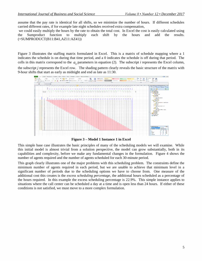
function. Figure 13 shows a five linear segment approximation. If a decision variable is maximized but

constrained to be less than each of these segments, it provides a reasonable approximation of the TSF curve.

Figure 14 shows the actual TSF curve and the piecewise linear approximation on the same graph demonstrating

the close fit for TSF levels above about 20%.

Figure 13 – Piecewise Linear Segments

-10%

10%

30%

50%

70%

90%

110%

130%

150%

0 5 10 15 20 25 30 35 40 45

Serv

ice

Le

vel R

esu

lt (

TSF)

Agent's Staffed

Service Level as a Function of Staffing

-50%

-30%

-10%

10%

30%

50%

70%

90%

110%

130%

150%

0 5 10 15 20 25 30 35 40 45

Serv

ice

Leve

l Res

ult

(TS

F)

Agent's Staffed

Piecewise Linear Approximation


12

Figure 14 – Piecewise Linear Approximation

We can then formulate a model with the following definitions:

Sets

I: time periods

J: possible schedules

H: segments in the linear approximation

Decision Variables

xj: number of resources assigned to schedule j

Model Parameters

cj: cost of schedule j

aij: indicates if schedule j is staffed in time i

g: global SLA goal

mih: slope of piecewise TSF approximation h

in period i

bih: intercept of piecewise TSF approximation

h in period i

i: minimum number of agents in period i

ni: number of calls in period i

State Variables

yi: service level achieved in period i

The model can then be expressed as

min j j

j J

c x

(4)

subject to

ij j i

j J

a x

i I (5)

i ih ij j ih

j J

y m a x b

,i I h H (6)

i i i

i I i I

y n g n

(7)

,j ix y ,i I h H (8)

The objective function (4) is the same as model 1, minimizing the weighted cost of schedules staffed. Constraint

(5) requires the staffing in each period to be large enough to ensure the minimum period by period service level is

achieved. Note that the parameter i is defined statically as the number of agents required to achieve the target

minimum service level. We perform this calculation in Excel using the Staff to TSF function, a custom function

coded in Visual Basic it searches for the minimum number of agents required to achieve the specified service

level. These calculations are based on approximate formulas for the Erlang A model presented in Mandelbaum &

Zeltyn (2004). Constraint (6) constrains the real-valued decision variable yi to be less than each of the piecewise

linear segments. The process of finding the lowest cost solution that satisfies the global constraint will force the

yi values to make the piecewise constraint binding. Constraint (7) enforces the global TSF requirement, if forces

the sum of each period’s TSF and its calls to be greater than the sum of all calls and the global TSF requirement.

-60%

-40%

-20%

0%

20%

40%

60%

80%

100%

120%

0 5 10 15 20 25 30 35 40 45

Serc

ice

Leve

l Res

ult

(TS

F)

Agents Staffed

Piecewise Linear Approximation

TSF

PWL TSF



13

Constraint (8) specifies that the agents assigned to each schedule are non-negative integers and the service level in

each period is a non-negative real number.

Compared to model 1 this model requires additional decision variables and constraints to facilitate the piecewise

linear calculation of the service level. However, the additional decision variables are real valued so there is no

impact on the number of schedules we can include. In this model formulation we have one integer variable for

each schedule. The number of real valued variables required is equal to the number of time periods plus one for

the overall service level. The number of constraints is equal to the number of time periods multiplied by one plus

the number of piecewise segments. One constraint is required for the per-period minimum service level, and an

additional constraint is required for each piecewise segment per time-period.

4.1 Results

To evaluate model 2 we solve the same 6 instances we used for model one, summarized in Table 2. When solving

model one, we used the number of agents as an input parameter. In model two we use the number of calls per

period that will generate the same number of agents. The call volumes forecasts and schedule options as in model

1. Staffing requirements in model 1 are defined based on an 80% TSF requirement. The only policy change we

make is that we now require an 80% TSF service level requirement over the course of the week, but allow for a

65% TSF in any individual period. The TSF calculation is based on the Erlang A model assuming calls have an

average talk time of 12 minutes, that callers have an average time to abandon of 300 seconds. The service level

requirement is to answer 80% of all call within 60 secs, and 65% of calls within 60 seconds for every 30-minute

period.

Table 2 – Instance Summary

The time required to solve model 2 instances is significantly longer than the time required for model 1. Size

statistics and representative solution times are presented in

Table 3. Solution times for our data ranged from 9.5 seconds to nearly 6 minutes.

Table 3 – Model 2 Summary

The ability to schedule to a global service requirement reduces total staffing costs as summarized in Table 4. The

cost savings range from 3.6% to 10%. The intuition behind this savings is easy to understand; by no longer

having to match the service level in each period the optimization model gains significant flexibility to match

supply and demand. It is this same added flexibility that makes the model much more difficult to solve to

optimality.

Instance Description

Instance 1 Simple Day Schedule

Instance 2 Simple 5 Day Schedule

Instance 3 24x7 Full Time 5 day schedule

Instance 4 24x7 Full Time 4 and 5 day schedules

Instance 5 24x7 Flexible Staffing

Instance 6 24x7 Flexible Staffing with Explicit Breaks

1 2 3 4 5 6

Time Periods 48 240 336 336 336 336

Possible Schedule DVs 31 31 336 1680 3696 18816

Implemented Schedules DVs 31 31 336 1680 2000 2000

PW Linear DVs 48 240 336 336 336 336

Total DVs 79 271 672 2016 2336 2336

Constraints 289 1441 2017 2017 2017 2017

Bounds 79 271 672 2016 2336 2336

Representative Solution Time (secs) 9.52 47.8 142 255 237 353

% Gap Setting 0.0% 0.0% 2.0% 3.5% 2.0% 5.0%


14

Table 4 – Model Comparison

Figure 15 – Period by Period Service Level

The graph in Figure 15 shows the period by period service level. The service level is seen to vary from the period

minimum of 65% to 100%. Allowing the period by period service level to drop as low as 65% creates a situation

where the service level varies significantly over the course of the week, as shown in Figure 15. This phenomenon

is better illustrated in Figure 16 and Figure 17. In these figures we show only one day worth of data. In each

graph we superimpose expected call volume as a line with a separate scale. In Figure 16 we see that the service

level is allowed to drop off during several periods, including the peak demand period in the late morning.

Figure 17 shows that we still reach a maximum staffing level during the peak demand period, but the ability to

attenuate that peak somewhat allows us to lower overall costs. The ability of the global service level model to

better match supply and demand seems to explain why the cost improvement afforded by this model is most

significant for instances of Model One where the excess staffing percentage is the highest. This implies two

alternative strategies for call center managers to reduce costs. First, increase scheduling flexibility by adding

more scheduling options, through part time shifts and other non-standard scheduling patterns such as 4x10 shifts.

Second, increase scheduling options by implementing a global service level requirement with a relaxed period by

period requirement. Each approach has its own challenges and complexities, but it appears either can help reduce

the cost of service delivery.

Model 1 Model 2 % Reduction

Instance 1 180.00 162.00 10.0%

Instance 2 1,170.00 1,080.00 7.7%

Instance 3 1,280.00 1,160.00 9.4%

Instance 4 1,160.00 1,080.00 6.9%

Instance 5 1,104.00 1,064.00 3.6%

Instance 6 1,143.50 1,098.50 3.9%

Hours

0.00

0.20

0.40

0.60

0.80

1.00

1.20

1 8

15

22

29

36

43

50

57

64

71

78

85

92

99

10

6

11

3

12

0

12

7

13

4

14

1

14

8

15

5

16

2

16

9

17

6

18

3

19

0

19

7

20

4

21

1

21

8

22

5

23

2

23

9

24

6

25

3

26

0

26

7

27

4

28

1

28

8

29

5

30

2

30

9

31

6

32

3

33

0

Period by Period Service Level



15

Figure 16 - Period by Period SL and Call Volume

Figure 17-Period by Period Staffing and Call volume

5 Conclusions and Future Research

In this paper we have examined two computationally intensive call center scheduling models, formulated in

Excel. We have examined the impact scheduling flexibility has on computational effort as well as overall costs.

We examined two primary forms of flexibility. First, we created a larger menu of schedules from which to pick

by adding different types of shift patterns. Given the seasonal nature of call center demand, both within a day and

across a week, this flexibility provided significant benefits. With more options to choose from the scheduling

algorithm was able to reduce the number of agents scheduled above and beyond what was required from 36.8% to

7.5%. The second type of flexibility we investigated deals with the nature of the call center’s service level

agreement. By partially relaxing the period by period service level requirement, while still enforcing an overall

global service limit, the call center can also address the difficulty associated with demand spikes.

Incorporating this type of flexibility requires a significant modification to the relatively simple set covering

model. The computational requirements for this model are significantly higher than they were for the first model,

but this approach will further reduce staffing costs. We have also shown that Excel with Risk Solver Platform is a

viable platform for solving these models to near optimality in reasonable time frames. Our analysis showed that

the global service level constraint allowed us to achieve a lower cost solution. In our analysis we allowed the

80% service level target to slip to 65% in individual time periods. We saw cost improvements that ranged from

3.6% to 10%. A more complete analysis would assess the factors that drive this improvement and examine how

the per-period minimum service level requirement impacts the total savings.

0

10

20

30

40

50

60

0%

10%

20%

30%

40%

50%

60%

70%

80%

90%

100%

1 2 3 4 5 6 7 8 9 101112131415161718192021222324252627282930313233343536373839404142434445464748

Period by Period Service Level and Expected Call Volume

TSF

Expected Calls

0

10

20

30

40

50

60

0

5

10

15

20

25

1 2 3 4 5 6 7 8 9 101112131415161718192021222324252627282930313233343536373839404142434445464748

Period by Period Staffing and Expected Call Volume

Scheduled

Expected Calls


16

6 References

Aykin, T. (1996). Optimal Shift Scheduling with Multiple Break Windows. Management Science, 42(4), 591-602.

Bechtold, S. E., & Jacobs, L. W. (1990). Implicit Modeling of Flexible Break Assignments in Optimal Shift

Scheduling. Management Science, 36(11), 1339-1351.

Brusco, M. J., & Jacobs, L. W. (1998). Personnel Tour Scheduling When Starting-Time Restrictions Are Present.

Management Science, 44(4), 534-547.

Brusco, M. J., & Jacobs, L. W. (2000). Optimal Models for Meal-Break and Start-Time Flexibility in Continuous

Tour Scheduling. Management Science, 46(12), 1630-1641.

Brusco, M. J., & Johns, T. R. (1996). A sequential integer programming method for discontinuous labor tour

scheduling. European Journal of Operational Research, 95(3), 537-548.

Dantzig, G. B. (1954). A Comment on Edie's "Traffic Delays at Toll Booths". Journal of the Operations Research

Society of America, 2(3), 339-341.

Gans, N., Koole, G., & Mandelbaum, A. (2003). Telephone call centers: Tutorial, review, and research prospects.

. Manufacturing & Service Operations Management, 5(2), 79-141.

Grossman, T. A., & Özlük, Ö. (2009). A Spreadsheet Scenario Analysis Technique That Integrates with

Optimization and Simulation. INFORMS Transactions on Education, 10(1), 18-33.

doi:10.1287/ited.1090.0027

Grover, J., & Lavin, A. M. (2007). Modern Portfolio Optimization: A Practical Approach Using an Excel Solver

Single-Index Model. The Journal of Wealth Management, 10(1), 60-72,68.

Gurgur, C. Z., & Morley, C. T. (2008). Lockheed Martin Space Systems Company Optimizes Infrastructure

Project-Portfolio Selection. Interfaces, 38(4), 251-262.

Henderson, W. B., & Berry, W. L. (1976). Heuristic Methods for Telephone Operator Shift Scheduling: An

Experimental Analysis. Management Science, 22(12), 1372-1380.

Kumiega, A., & Van Vliet, B. (2008). Optimal Trading of ETFs: Spreadsheet Prototypes and Applications to

Client-Server Applications. Interfaces, 38(4), 289-299.

LeBlanc, L. J., & Galbreth, M. R. (2007). Implementing Large-Scale Optimization Models in Excel Using VBA.

Interfaces, 37(4), 370-382. doi:10.1287/inte.1060.0256

LeBlanc, L. J., & Grossman, T. A. (2008). Introduction: The Use of Spreadsheet Software in the Application of

Management Science and Operations Research. Interfaces, 38(4), 225-227.

Mandelbaum, A., & Zeltyn, S. (2004). Service Engineering in Action: The Palm/Erlang-A Queue, with

Applications to Call Centers Draft, December 2004.

Ovchinnikov, A., & Milner, J. (2008). Spreadsheet Model Helps to Assign Medical Residents at the University of

Vermont's College of Medicine. Interfaces, 38(4), 311-323.

Pasupathy, K. S., & Medina-Borja, A. (2008). Integrating Excel, Access, and Visual Basic to Deploy Performance

Measurement and Evaluation at the American Red Cross. Interfaces, 38(4), 324-337.

Patterson, M., & Harmel, B. (2001). Using Microsoft Excel Solver for linear programming assignment problems.

International Journal of Management, 18(3), 308-313.

Patterson, M., & Harmel, B. (2002). An algorithmic approach for solving linear programming transportation

problems using Microsoft Solver. International Journal of Business Disciplines, 12(1), 1-5.

Patterson, M. C., & Harmel, B. (2003). An Algorithm for Using Excel Solver© for the Traveling Salesman

Problem. Journal of Education for Business, 78(6), 341-346. doi:10.1080/08832320309598624

Perzina, R., & Ramík, J. (2014). Microsoft Excel as a Tool for Solving Multicriteria Decision Problems. Procedia

Computer Science, 35, 1455-1463. doi:http://dx.doi.org/10.1016/j.procs.2014.08.206

Ragsdale, C. T. (2017). Spreadsheet Modeling & Decision Analysis: A Practical Introduction to Management

Science (8 ed.).

Robbins, T. R. (2010). Tour Scheduling and Rostering. In J. J. Cochran, L. A. Cox, P. Keskinocak, J. P.

Kharoufeh, & J. C. Smith (Eds.), Wiley Encyclopedia of Operations Research and Management Science:

John Wiley & Sons, Ltd.

Robbins, T. R., & Harrison, T. P. (2010). A stochastic programming model for scheduling call centers with global

Service Level Agreements. European Journal of Operational Research, 207, 1608-1619.

Sil, B. S., Banerjee, P., Kumar, A., Bui, P. J., & Saikia, P. (2013). Use of Excel-Solver as an Optimization Tool in

Design of Pipe Network. International Journal of Hydraulic Engineering, 2(4), 59-63.



17

Thompson, G. M. (1995). Improved Implicit Optimal Modeling of the Labor Shift Scheduling Problem.

Management Science, 41(4), 595-607.

Complexity and Flexibility in Call Center Scheduling Models

Documents

Transcript of Complexity and Flexibility in Call Center Scheduling Models