Geophys. J. Int. (1991) 107, 597-604

Complex component analysis of shear-wave splitting: theory

Xiang-Y ang Lil y2 and Stuart Crampin’1 Edinburgh Anisotropy Project, British Geological Survey, Murchison House, West Mains Road, Edinburgh EH9 3LA, UK2 Department of Geology and Geophysics, University of Edinburgh, James Clerk Maxwell Building, Edinburgh EH9352, UK

Accepted 1991 June 12. Received 1991 June 11; in original form 1991 January 8

SUMMARYThe use of complex arithmetic is a natural way to treat vectorially polarized data,where the real and imaginary components can be taken as two perpendicular axes.This transforms multicomponent data from conventional Cartesian coordinates topolar coordinates, and allows the calculation of instantaneous amplitude andinstantaneous polarization. We call this technique complex component analysis.Wave motion can be represented by instantaneous attributes which show distinctfeatures characteristic of the type of wave motion. It is particularly informative toexamine shear-wave splitting by instantaneous attributes. The instantaneous ampli-tude of shear-wave splitting has a number of local maxima, and the instantaneouspolarization has a combination of rectangular and semitriangular shapes. Shear-wave splitting can be identified from displays of instantaneous amplitude andpolarization, where the polarization of the faster split shear wave and the delaybetween the two split shear waves can be quantified from colour-coded displays. Theinstantaneous attributes can be displayed as wiggle-lines of amplitude superimposedon a colour-coded polarization, where the use of colour improves the indentificationand quantification of shear-wave splitting.

Key words: complex components, instantaneous amplitude, instantaneous polariza-tion, shear-wave splitting.

1 I N T R O D U C T I O N

Shear-wave splitting occurs along almost all ray paths in theuppermost 10 to 20 km of the Earth’s crust (Crampin 1985a,1987; Crampin & Atkinson 1985), including most sedimen-tary basins (Alford 1986; Willis, Rethford & Bielanski1986). We present a technique (Li & Crampin 1990a,1990b), which we shall call complex component analysis, toanalyse shear-wave splitting in multicomponent reflectionand VSP surveys.

Rene et al. (1986) extended complex trace analysis(Taner & Sheriff 1977; Taner, Koehler & Sheriff 1979) tomulticomponent data. They defined the complex multicom-ponent trace with real orthogonal components andimaginary (quadrature) components derived by applicationof the Hilbert transform to the corresponding realcomponents. They then defined several polarizationattributes including phase difference, reciprocal ellipticityand tilt angle. They applied the technique to multicom-ponent walkaway seismic data to characterize ambient noiseand source-generated waves.

Here, we directly define the two horizontal components ofmulticomponent reflection and VSP surveys as the real andimaginary parts of a complex component. This transforms

multicomponent data from conventional Cartesian coordin-ates to polar coordinates, and allows the calculation ofinstantaneous amplitude and instantaneous polarization.These quantities, referred to as seismic attributes (followingTaner et al. 1979), can be presented in conventional seismictime-versus-offset displays in which colour is used toquantify the polarizations of the shear waves.

Three major applications of such complex componentanalysis can be envisaged as follows.

(1) Anisotropic interpretation. Attributes can assist in therapid recognition and identification of shear-wave splittingin seismic sections, and in extracting shear-wave polariza-tions and delays from seismic data for interpretation interms of the crack- and stress-geometry throughout thereservoir.

(2) Stratigraphic interpretation. Seismic attributes pro-vide further information about the location and analysis offaults, discontinuities, unconformities, and other geologicalfeatures, as demonstrated by Taner et al. (1979).

(3) Hydrocarbon determination. Attributes can assist inrecognizing and interpreting bright spots, with particularapplication to the relative brightness of differentialshear-wave amplitude. Such bright spots are likely to be

597

598 X.-Y. Li and S. Crampin

associated with hydrocarbon accumulations in orientedcracks and fractures. Attributes can also help in interpretingfracture zones, and identifying lateral variation of fractureintensity, which may be related to preferential permeability.

This paper presents the theory of complex componentanalysis of shear-wave splitting. The paper suggeststechniques for estimating the behaviour of shear waves, anddemonstrates the significance of instantaneous attributes inidentifying and evaluating shear-wave splitting.

2 S I G N I F I C A N C E O F T H E C O M P L E XCOMPONENT

2.1 Definitions

We assume a multicomponent shear-wave data set with thehorizontal in-line x(t) and cross-line y(t) recording geometryshown in Fig. 1. We may write the horizontal displacementof a shear wave (or any seismic wave), with vectordisplacement Pt, amplitude A(t) and angle to the inlinedirection 0(t), as

x(t) = A(t) cos O(t)

and

(1)

y(t) = A(t) sin e(t). (2)

Thus, x(t) and y(t) can be considered as the real andimaginary parts of a complex signal z(t) = x(t) + iy (t),where i is the square root of -1. In this way, the method ofcomplex trace analysis of single component data (Taner &Sheriff 1977; Taner et al. 1979) can be extended tomulticomponent data without using the Hilbert transforms(Rene et al. 1986). Solving for A and 8 for any x and y, wehave

A(t) = [x2(t) + ~~(t)]l’~ = Iz(t)l, (3)e(t) = arctan [y(t)/x(t)], (4)

defined for f180”; where A(t) is the instantaneousamplitude; and 0(t) is the instantaneous polarization.

2.2 Physical significance

In addition to the attributes described above, the wavetrainalso contains information about instantaneous frequency,apparent polarity, energy distribution, and waveform, which

Figure 1. Diagram showing the coordinate system for complexcomponent analysis. Pt is the horizontal displacement of a shearwave at time 5 with amplitude A(t) and angle O(t) to the inlinedirection, and x(t) and y(t) are the coordinates of the twohorizontal components in a Cartesian coordinate system.

can also be extracted from complex components (Taner etal. 1979; Huang 1989). Each piece of information has aparticular significance and application in explorationseismology, and in reservoir characterization and develop-ment. Here, we shall only discuss instantaneous amplitudeand instantaneous polarization.

Instantaneous amplitude

The instantaneous amplitude in equation (3) is a measure ofthe distance between the moving particle and its equilibriumposition. Instantaneous amplitude may have its maximum atpoints other than at peaks or troughs of the two individualhorizontal components. Local maxima of instantaneousamplitude indicate the largest distance of the particle fromits equilibrium position, and may help in identifying theonset of the shear-wave signal and the interference of splitshear waves without rotating seismogram axes.

Instantaneous polarization

The instantaneous polarization in equation (4) is a measureof the polarization direction of the moving particle relativeto the polarization direction of the source. Since thepolarization is independent of amplitude, it may give clearparticle motion directions even for weak arrivals as long asthey are coherent signals. Thus, instantaneous polarizationmay be a good indicator of discontinuities, faults, pinchouts,and angularities, as demonstrated in similar circumstancesby Taner et al. (1979).

The variation of the instantaneous polarization ofrecorded split shear waves represents the variation of thedirection of the particle motion of the split shear waves. Thefirst arrival of the split shear waves is polarized in a directionfixed by the ray path through the anisotropic rock (Crampin1981), so that the instantaneous polarization tends to remainconstant until the arrival of the slower split shear wave.Thus the polarization display, and associated amplitudedisplay, can help to identify and quantify shear-wavesplitting in both seismic reflection and VSP data sets.

2.3 Represention of wave motion

Figures 2(a) and (b) show the seismograms and instan-taneous amplitude and polarization attributes of eighttypical wave motions: linear, elliptical, and shear-wavesplitting with six different time delays. Fig. 3 showscorresponding polarization diagrams (hodograms) of theparticle motion. Since any shear-wave motion in thehorizontal plane can be considered as either linearly, orelliptically polarized (or some combination thereof inshear-wave splitting), we first discuss these two characteris-tic types of wave motion.

Linear wave motion

WMl in Figs 2 and 3 show typical linear motion, that can bewritten as

y(t) =x(t) tan a, (5)where x(t) and y (t) are the displacements in the x and ydirections, respectively; a is the angle the polarization

Complex component analysis: theory 599

WMl

WM2

WM3

WM4

WM5

WM6

WM7

WM8

r:!:!:!0 . 0 0 0 . 0 5 0 . 1 0 0 . 1 5

T I M E , S E C O N D S

(a)

AP

AP

AP

AP

AP

AP

AP

AP

0 . 0 0 0 . 0 5 0 . 1 0 0 . 1 5

T I M E , S E C O N D S

(b)

Figure 2. Seismograms and instantaneous attributes of eight typicalwave motions. WMl is linear motion, WM2 is elliptical, and WM3to WM8 show shear-wave splitting with time delays increasing from8 ms (WM3) to 48 ms (WM8) for a 40Hz signal. (a) Horizontalcomponent seismograms, X inline and Y crossline; (b) displays ofinstantaneous amplitude (A) and polarization (P). Arrows on WM2mark the position of the effective polarization angle, and arrows onWM3 to WM8 mark the points where the polarization changesdirection at the onset of the second split shear-wave arrival.

DELAYS

WMl

WM2

WM3

WM4

WM5

WM7

0 . 0 0 0.15Figure 3. Polarization diagrams of the eight typical wave motions inFig. 2. The small arrows mark the direction of motion, and the largearrows mark the initial polarization directions.

makes with the inline direction. In Fig. 2, ar is chosen as160” measured from the instantaneous polarization directionto the inline direction:

a = 160”, x(t) < 0,e(t) = 0, x(t) = 0, (6)

a - n = 160” - 180” = -2O”, x(t) > 0.

We see that the instantaneous polarization of linearmotion is a series of rectangular shapes. The importantfeatures to note are as follows.

(1) The height or depth of the initial rectangle from thebase line is the polarization angle of the linear motion atthat point, and the height or depth of the next rectangle isthe polarization angle less 180”. Note that there is only onerectangle unless the signal is more than half a cycle long.

(2) The width of the rectangle is the half period of thewave motion, independent of the number of cycles in thewaveform (as long as the signal contains at least half acycle). Thus, the angle of polarization given by theinstantaneous polarization in Fig. 2(b) is 160”, and theinstantaneous amplitude has two local maxima. The finalnarrower rectangle in WMl, Fig. 2(b), is a result of thelow-amplitude tail of the wavelet used in Fig. 2(a).

Elliptical motion

The elliptical motion WM2 in Figs 2(a) and 3 can berepresented by

y(t) = a sin wt, x(t) = b cos (ut + q5), (7)

where a and b are the peak amplitudes in y and xcomponents (WM2, Fig. 2a), respectively; cr) is the angularfrequency, here taken to be 2~ x 40, say, for a 40 Hz signal,and C#J is a phase shift, here taken to be 20”.

The elliptical motion in Fig. 2(b) gives a varyinginstantaneous polarization of repeated characteristic shapes,which we call ‘semitriangular’. The polarization angle of theellipse (the direction of semimajor axis, also called theeffective polarization angle) can be determined bycombining the instantaneous amplitude displays. Themaximum amplitude occurs when the particle displacementis at the long axis of the ellipse. Thus, the angle at the timewhere the amplitude has a local maximum is an effectivepolarization angle. (Note, however, that this is not usuallycoincident with the polarization directions of either of thesplit shear waves.) There is also another feature which canbe used to determine the polarization angle of the ellipse.When the particle motion is at the maximum, thepolarization has a smooth variation which forms a step inthe instantaneous polarization [marked with arrowhead inWM2, Fig. 2(b)]. The polarization angle can be estimatedfrom the amplitude of this step.

The features discussed above can be used to determinethe type of wave motion. Wholly rectangular shapes indicatelinear motion (or well-separated split shear waves), andsemitriangular shapes indicate some form of ellipticalmotion. Note that if black and white plots of instantaneouspolarization, as in Fig. 2(b), were to be routinely used todetermine polarization angles, the polarization would needto be plotted at a larger scale so that the values of the

600 X. -Y. Li and S. Crampin

polarization would be easily read. More effective displayswill be discussed below.

3 S H E A R - W A V E S P L I T T I N G

The most characteristic features of shear waves inanisotropic structures are the polarization anomalies in the3-D waveforms resulting from shear waves splitting intophases which propagate with different polarizations anddifferent velocities (Crampin 1978, 1981; Crampin & Booth1985). The polarization patterns of shear-wave splitting canbe represented by the interference of two linear motionswith (typically) similar waveforms but different polarizationdirections and separated by a time delay. The interferenceof these signals results in a combination of linear andelliptical waveforms, or two linear waveforms if the timedelay between the two split shear waves is large enough toseparate the signals. The patterns of particle motion varywith the delay and particle-motion polarizations of the twosplit shear waves.

We examine a variety of characteristic wavetypes.Without loss of generality, we assume in this paper that thetwo split shear-wave polarizations are polarizedorthogonally.

3.1 Polarization patterns

The six polarization patterns, WM3 to WM8 in Fig. 3, arecharacteristic of shear-wave splitting with a range of delays:from WM3 to WM8, the delay linearly increases from 8 to48 on a 40 Hz signal (phase delays from 72” to 432”,respectively). At the onset of the faster split shear waves,the polarizations are linear. At the onset of the slower shearwaves, the polarizations either change smoothly to ellipticalmotion or change abruptly to further linear motion indifferent directions, if the delays between the two split shearwaves are sufficiently large. When the delays between thesplit shear waves are less than half a cycle (as in WM3 andWM4, Fig. 3), the polarizations change smoothly withelliptical patterns of polarization, and the underlyingcharacteristic cruciform patterns are barely discernible. Asthe delays increase beyond half a period (WM5 and WM6),the polarizations change more sharply, and the cruciformpatterns become clearer. When the delays are equal to theperiod of the wave (WM7), or greater (WM8), thepolarizations change abruptly, and the patterns are whollycruciform.

3.2 Instantaneous attributes

Figure 2(b) shows corresponding instantaneous attributes ofamplitude (A) and polarization (P) of the seismograms inFig. 2(a) and polarization diagrams in Fig. 3.

WM3 and WM4

The amplitude has three local maxima, and the polarizationstarts with a step equal to the polarization angle of the firstarrival. The polarization then remains constant until theslower wave arrives, when it changes smoothly. If thechange can be identified [marked by arrowheads in WM3and WM4. Fig. 2(b)], the arrival time and polarization

direction of the slower split shear wave and the delaybetween the two split shear waves can also be determined.The overall feature of the instantaneous polarization ofshear-wave splitting is a combination of rectangular andsemitriangular shapes.

WM5 and WM6

The amplitude has four local maxima, and the polarizationis again a combination of rectangular and semitriangularshapes. The polarization change on arrival of the slowershear wave has been marked by arrows in Fig. 2(b), but issubtle and difficult to identify reliably.

WM7and WM8

The amplitude has four clear local maxima, and thepolarization has wholly rectangular shapes. The polarizationdirections and the delay can be determined easily.

To summarize: as the delay increases, the number of localmaxima of instantaneous amplitude increases, and the shapeof instantaneous polarization changes from a combination ofrectangular and semitriangular shapes to a combination ofpurely rectangular shapes. Thus, shear-wave splitting can beidentified from displays of instantaneous amplitude andpolarization, and the polarization direction can be easily andaccurately determined when the delays are sufficiently large.The delays are easy to determine when the delays are large,but may be difficult to determine when the delays are lessthan a cycle. We shall see that colour displays of theattributes are more informative.

4 C O L O U R D I S P L A Y S

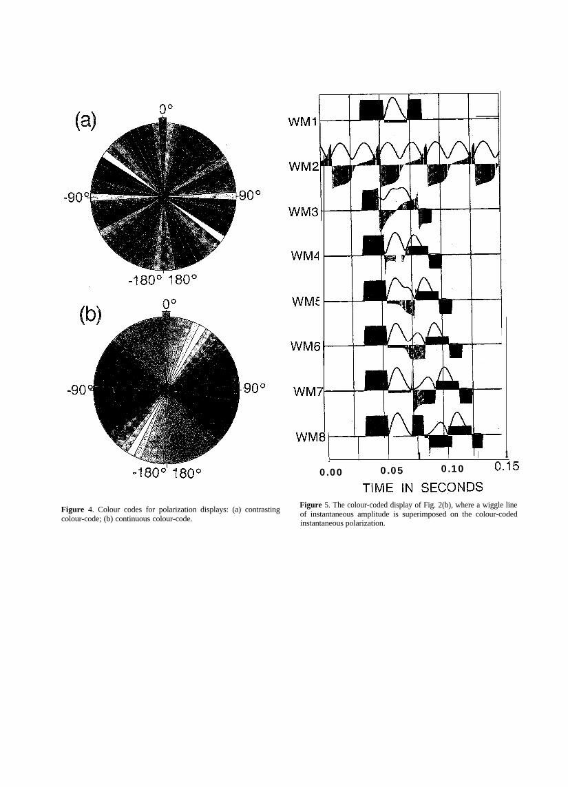
The use of colour in displaying seismic data has been shownto improve the perceptibility of subsurface features (Taneret al. 1979). Fig. 4 shows the colour codes used for displaysof instantaneous polarization in this paper. Code (a)contains a series of contrasting colours, useful for identifyingthe exact value of the polarization; and (b) a series ofcontinuous colours, useful for recognizing shear-wavesplitting on a larger scale. Note that the colours repeat every180”. Thus, if the polarization values have a difference off180”, they will be coded with the same colour, allowing forthe f180” difference between the positive and negativevalues of the polarization of linear motion.

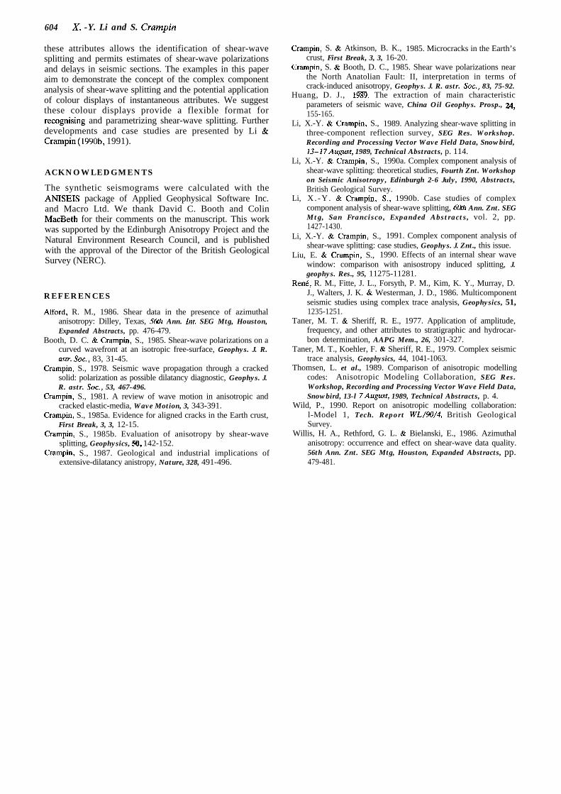
Figure 5 is the colour display of Fig. 2(b), showing thecolour-coded polarization angle in the contrasting colours ofcode (a) superimposed on a wiggle trace of instantaneousamplitude. This type of display aids estimation of theparameters of shear-wave splitting:

(1) The colour-coded polarization quantifies the polariza-tion direction by reference to the colour key. For exampleWMl is a wholly red colour, which represents 162” f 3” (or-18” f 3”), where we use the angle (colour) D to representthe range D - 3” < to I D + 3”. From the shape of thepolarization curve we know the angle is 162” f 3”.

(2) The onset of the slower arrival can be easily identifiedby the change of the uniform (red) to the varying colours ofelliptical motion in WM3 to WM7, or the uniform (black)

-go*

Figure 4. Colour codes for polarization displays: (a) contrastingcolour-code; (b) continuous colour-code.

WM1’

WMZ

WM4

WME

WM7

WM81 I I----l II I I I ’ I I 10.00 0.05 0.10 0.15

TIME IN SECQNDSFigure 5. The colour-coded display of Fig. 2(b), where a wiggle lineof instantaneous amplitude is superimposed on the colour-codedinstantaneous polarization.

d-C

T O

ii? I 01 I b ’ ? I zd

0 and

W LL7 c3 . I

EaNo33s Ni- 3w T--

m

saNo33s NI 3lAlIl

colour representing perpendicular motion (72” f 3” or- 108” f 3”).

(3) The difference between the linear motion. WMl andthe shear-wave splitting with a delay of more than a cycle,WM8, is clearly demonstrated by the colour. WMl has asingle colour which implies no change of polarization (or achange of &180”); whereas WM8 has two different colours(separated by approximately go”), which implies twoapproximately orthogonal linear motions.

In applying these techniques to seismograms withincoherent or signal-generated noise, the use of thecontinuous colour code, is recommended for identifyingshear-wave splitting, although the contrasting colour codemay be required for estimating values of polarization. In thefollowing examples, the polarization is coded by thecontinuous code (b). Two examples are used to demonstratethe significance and application of instantaneous attributesto anisotropic interpretations.

1990) to the Anisotropic Modelling Collaboration ofThomsen et al. (1989). A number of research groups arecontributing to the Anisotropic Modelling Collaboration(AMC) to calculate full wave synthetic seismograms ins p e c i f i e d VSPs a n d CMPs i n a given anisotropicmultilayered model (Thomsen et al. 1989). Fig. 6(a),adapted from Wild (1990), shows a schematic diagram ofModel 1 (AMCl) used in this study (note that only everysecond three-component geophone is marked in the figure).The crack strike is east-west in each anisotropic layer. Themodel features a strongly anisotropic layer from 1500 to2000 m depth, simulating highly fractured reservoir rocks.

5 A P P L I C A T I O N S

5.1 AMC model and data

AMC MODEL

The data used are a synthetic VSP and a CMP gather fromthe response of the Edinburgh Anisotropy Project (Wild

The collaboration calculated a full nine-component(inline, crossline, and vertical sources recorded by inline,crossline, and vertical receivers) offset VSP, and a varietyof nine-component reflection lines, as indicated in Fig. 6(a).Only one source component, the inline component, of boththe VSP, at an offset of 500 m and an azimuth of N45”E, andthe 2400 m reflection line data, again at an azimuth ofN45”E, are analysed here. Fig. 6(b) shows the twohorizontal components of the VSP excited by the inlinesource located at Sv in Fig. 6(a). Cruciform patterns ofparticle motion in the polarization diagrams from primarydownward propagating shear waves (polarization diagrams cand d) are observed within and below the simulated

Complex component analysis: theory 601

Figure 6. (a) The structure and geometry of the AMC model. The dots along survey lines represent every second geophone of 50 m geophonespacing. (b) The two horizontal components of the VSP data for the inline source orientation. The offset is 500 m at an azimuth of N45”E. Notenoise on the first five in-line source components. Some selected polarization diagrams are shown. Number on top right corner of thepolarization diagrams is the geophone number at the time interval marked below. Arrows drawn on particle motions are in the same notationas Fig. 3. Rl to R4 are reflected shear waves from Layers Ll to L4, respectively. Ml to M4 are the multiples of the primary downwardpropagating shear wave. The four particle motions on the left are selected from the primary downgoing shear waves, and on the right from thereflected shear waves. (c) The two horizontal components of the reflection line at an azimuth of N45”E for the inline source orientation withsome selected polarization diagrams. Symbols drawn on the diagrams have the same notation as (b). Those on the left are selected from thereflected shear waves Rl, R2, R3 and R4 at geophone 1 (near offset), and on the right from the same event-arrivals but at geophones at largeroffsets where the polarizations have changed.

602 X.-Y. Li and S. Crampin

INLINE CROSS LINE

i

0 . 9 0 1.10

INLINE C R O S S L I N E

0 . 3 5 0 . 5 5

d, ’T-l7 Y

I I I

1.60 i .a0

2.0

0 . 5 0 0 . 7 0

i .a5 2 . 0 5

Figure 6. (continued)

fractured reservoir (Layer L4); the delays between thedownward shear waves gradually increase with increasinggeophone depth. Fig. 6(c) shows the two horizontalcomponents of the CMP gather excited by the inline sourcelocated at S, in Fig. 6(a). Polarization diagrams of theshear-wave reflection from the bottom of the reservoir(event R4; polarization diagrams d and h) have cruciformpolarizations and show strong shear-wave splitting.

5.2 Analysis of the VSP

Figure 7 shows the colour-coded display for the instan-taneous polarization of the VSP data in Fig. 6(b), with asuperimposed wiggle trace of instantaneous amplitude. Thedisplay contains a large amount of relatively easilyinterpretable information. A few major items in theinterpretation of the display are summarized as follows.

(c)

(1) Event A corresponds to the P-wave arrival in Fig.6(b). The whole waveform of the instantaneous amplitude iscovered by a single green colour, implying linear motionwith a polarization angle of 0” f 3” (or f180 f 3”).

(2) Event B is the direct shear wave. Shear-wave splittingcan be clearly identified by the shape of polarization curvecontaining two rectangles of blue (132” f 3” or -48 f 3”) andorange (42” f 3” or -138” f 3”) representing orthogonal ornearly orthogonal motion. The polarization direction of thefaster shear wave is represented by the blue rectangle(-48” f 3” or 132” f 3”), and the magnitude of the delay canbe estimated from the duration of the blue rectangle. Belowgeophone 30, at the top of layer L4, the duration of the bluerectangle gradually increases, showing the delay betweenthe split shear waves increasing with depth in the stronglyanisotropic reservoir.

(3) Event C corresponds to R2, a reflection from the

Complex component analysis: theory 603

bottom of L2. Shear-wave splitting can also be identified bythe change of colours from blue to orange. Because thedelay is small, this change is subtle and can only be clearlyseen at geophones 9,10,11, and 12, where there is a narrowband of blue.

(4) Event D corresponds to R3, a reflection from thebottom of L3. The blue rectangle covering the waveformindicates linear motion with a polarization angle of 132” f 3”(or -48 f 3”).

(5) Event E corresponds to R4, a reflection from thebottom of L4. The waveforms of instantaneous amplitudeare dominated by two rectangles of blue and orange, andthe shear-wave splitting can be identified and parametersestimated as for the direct shear wave.

(6) Events F and G correspond to Ml and M2,respectively, multiples of the primary down shear wave. Theshape of the polarization curve and the variation of colourshow the same features as those of the direct shear wave.

5.3 Analysis of the CMP gathersFigure 8 shows the instantaneous attributes of Fig. 6(c)displaying colour-coded polarization data superimposed bywiggle lines of instantaneous amplitudes. The instantaneousattributes of CMP gathers have two applications.

First, as discussed in the VSP data, the attributes of theCMP gathers can be used to identify the type of shear-wavemotion in reflected waves, as follows.

(1) Events A and F, describing the P-wave reflectionsfrom the bottom of layers Ll and L3, respectively, showlinear motion as they are both dominated by a single lightgreen (0” f 3” or f180” f 3”) and dark green (174” f 3” or-6” f 3”) colours, respectively.

(2) Events C and G (corresponding to Rl and R3,shear-wave reflections from the bottom of layers Ll and L3,respectively) are also linear motions at near offset and aredominated by one major colour: event C by the backgroundgreen (0” f 3” or f 180” f 3”), and G by blue (132” f 3” or-48” f 3”).

(3) Events E and H, corresponding to R2 and R4, areshear-wave reflections from the bottom of L2 and L4,respectively, and at near offsets both show shear-wavesplitting which can be recognized by the shape of thepolarization curve and the variation of colour from blue toorange. The polarization and delay can be determined in thesame way as discussed for the VSP data. The delay of eventE is small as indicated by the narrow blue rectangle, but thedelay of event H is large as it traverses the stronglyanisotropic L4 on both downgoing and upgoing rays.

Secondly, the attributes of CMP gathers containinformation about the effective shear-wave window at thefree surface (Booth & Crampin 1985) for each shear-wavereflection:

(1) The polarization of the shear wave changes withoffset, as demonstrated by the variation of colour. Forexample, event B (a P-S conversion from the bottom oflayer Ll) starts with background green colour at near offset,then changes to a light green at middle offset, and becomesyellow at far offset, indicating an approximate 30” change inpolarization as the angle of incidence on the reflectinginterface varies (Liu & Crampin 1990). In contrast, the

polarization of the P-wave is relatively unaffected by thevariation of offsets as shown by events A and F.

(2) ‘Critical angles’ at internal interfaces can also beidentified, where one of the shear waves has zero reflectionamplitude as the offset increases (Liu & Crampin 1990). Forincidence on the reflecting interface smaller than this angle,the colour of the instantaneous polarization remainsconstant (or only shows gradual change), but at the criticalangle the colour indicates a 90” polarization (phase) change.For example, the change due to the critical angle forreflection from Layer 1 for event C is at geophone 12 (thecolour suddenly changes from green to red, indicating a 90”change), and the critical angle for reflection from Layer 2for event E is at geophone 22. Similarly, there are criticalangles for event G at geophone 28, and elsewhere.

Effects of the shear-wave window are difficult to observebecause of the interference of multiply reflected andconverted waves. Note that effects of the first ‘critical angle’at internal reflections typically cause a comparatively simplechange in polarization direction, and hence a change in theinstantaneous polarization (Liu & Crampin 1990), whereasthe shear-wave window at the surface usually causes muchmore complicated effects (Crampin & Booth 1985).

Identifying the offset at which the polarization of eachshear-wave arrival changes polarity is important for stackingthe CMP gather. Conventional stacking of split shear waves,where the polarizations and delays change markedly withoffset, will tend to distort and degrade the characteristics ofthe split shear waves unless appropriate techniques are used(Li & Crampin 1989). Such changes of polarity occur both atcritical reflections at internal interfaces (Liu & Crampin1990), and at the surface shear-wave window (Booth &Crampin 1985).

6 DISCUSSION AND CONCLUSIONS

We have suggested a technique for the complex componentanalysis of shear-wave data by transforming the displace-ments from Cartesian to polar coordinate systems. The useof colour provides a technique for displaying the largeamount of information contained in the shear wavetrain(Crampin 1985b) in a form which is similar to manyconventional time-versus-offset displays, and which couldeasily be assimilated into conventional stratigraphic analysis.

The VSP example shows how the technique can help inanalysing and estimating shear-wave splitting continuouslyas it varies with depth. The results of pre-stack reflectiondata show how shear-wave splitting can be traced along bothtime and offset directions, and reveals the potential forapplying these techniques to post-stack data, so that muchof the stratigraphic and anisotropic interpretation can bemade on a single display of complex attributes. Althoughthe instantaneous attributes were defined for verticalpropagation, at wider angles they can be used to identify thevarious critical angles at the surface and at internalinterfaces, which are critical for any stacking of shear-wavedata in anisotropic structures (Li & Crampin 1989).

We conclude that the treatment of the two horizontalcomponents in multicomponent shear-wave data as acomplex variable allows convenient displays of instan-taneous amplitude and polarization. The colour display of

604 X. -Y. Li and S. Crampin

these attributes allows the identification of shear-wavesplitting and permits estimates of shear-wave polarizationsand delays in seismic sections. The examples in this paperaim to demonstrate the concept of the complex componentanalysis of shear-wave splitting and the potential applicationof colour displays of instantaneous attributes. We suggestthese colour displays provide a flexible format forrecognising and parametrizing shear-wave splitting. Furtherdevelopments and case studies are presented by Li &Crampin (1990b, 1991).

ACKNOWLEDGMENTS

The synthetic seismograms were calculated with theANISEIS package of Applied Geophysical Software Inc.and Macro Ltd. We thank David C. Booth and ColinMacBeth for their comments on the manuscript. This workwas supported by the Edinburgh Anisotropy Project and theNatural Environment Research Council, and is publishedwith the approval of the Director of the British GeologicalSurvey (NERC).

REFERENCES

Alford, R. M., 1986. Shear data in the presence of azimuthalanisotropy: Dilley, Texas, 565h Ann. Znt. SEG Mtg, Houston,Expanded Abstracts, pp. 476-479.

Booth, D. C. & Crampin, S., 1985. Shear-wave polarizations on acurved wavefront at an isotropic free-surface, Geophys. J. R.a&r. sot., 83, 31-45.

Crampin, S., 1978. Seismic wave propagation through a crackedsolid: polarization as possible dilatancy diagnostic, Geophys. J.R. astr. Sot., 53, 467-496.

Crampin, S., 1981. A review of wave motion in anisotropic andcracked elastic-media, Wave Motion, 3, 343-391.

Crampin, S., 1985a. Evidence for aligned cracks in the Earth crust,First Break, 3, 3, 12-15.

Crampin, S., 1985b. Evaluation of anisotropy by shear-wavesplitting, Geophysics, 50, 142-152.

Crampin, S., 1987. Geological and industrial implications ofextensive-dilatancy anistropy, Nature, 328, 491-496.

Crampin, S. & Atkinson, B. K., 1985. Microcracks in the Earth’scrust, First Break, 3, 3, 16-20.

Crampin, S. & Booth, D. C., 1985. Shear wave polarizations nearthe North Anatolian Fault: II, interpretation in terms ofcrack-induced anisotropy, Geophys. J. R. astr. Sot., 83, 75-92.

Huang, D. J., 1989. The extraction of main characteristic

Li,

Li,

Li,

Li,

parameters of seismic wave, China Oil Geophys. Prosp., 24,155-165.X.-Y. & Crampin, S., 1989. Analyzing shear-wave splitting inthree-component reflection survey, SEG Res. Workshop.Recording and Processing Vector Wave Field Data, Snowbird,13-17August, 1989, Technical Abstracts, p. 114.

X.-Y. & Crampin, S., 1990a. Complex component analysis ofshear-wave splitting: theoretical studies, Fourth Znt. Workshopon Seismic Anisotropy, Edinburgh 2-6 July, 1990, Abstracts,British Geological Survey.X . - Y . & Crampin, S., 1990b. Case studies of complexcomponent analysis of shear-wave splitting, 6@h Ann. Znt. SEGMtg, San Francisco, Expanded Abstracts, vol. 2, pp.1427-1430.X.-Y. & Crampin, S., 1991. Complex component analysis ofshear-wave splitting: case studies, Geophys. J. Znt., this issue.

Liu, E. & Crampin, S., 1990. Effects of an internal shear wavewindow: comparison with anisostropy induced splitting, J.geophys. Res., 95, 11275-11281.

Rend, R. M., Fitte, J. L., Forsyth, P. M., Kim, K. Y., Murray, D.J., Walters, J. K. & Westerman, J. D., 1986. Multicomponentseismic studies using complex trace analysis, Geophysics, 51,1235-1251.

Taner, M. T. & Sheriff, R. E., 1977. Application of amplitude,frequency, and other attributes to stratigraphic and hydrocar-bon determination, AAPG Mem., 26, 301-327.

Taner, M. T., Koehler, F. & Sheriff, R. E., 1979. Complex seismictrace analysis, Geophysics, 44, 1041-1063.

Thomsen, L. et al., 1989. Comparison of anisotropic modellingcodes: Anisotropic Modeling Collaboration, SEG Res.Workshop, Recording and Processing Vector Wave Field Data,Snowbird, 13-l 7August, 1989, Technical Abstracts, p. 4.

Wild, P., 1990. Report on anisotropic modelling collaboration:l-Model 1, Tech. Report WL/90/4, British GeologicalSurvey.

Willis, H. A., Rethford, G. L. & Bielanski, E., 1986. Azimuthalanisotropy: occurrence and effect on shear-wave data quality.56th Ann. Znt. SEG Mtg, Houston, Expanded Abstracts, pp.479-481.