COMPLETE -...
99
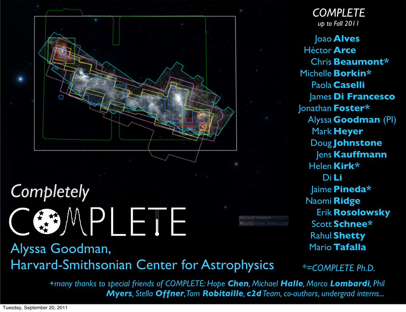
Joao Alves Héctor Arce Chris Beaumont* Michelle Borkin* Paola Caselli James Di Francesco Jonathan Foster* Alyssa Goodman (PI) Mark Heyer Doug Johnstone Jens Kauffmann Helen Kirk* Di Li Jaime Pineda* Naomi Ridge Erik Rosolowsky Scott Schnee* Rahul Shetty Mario Tafalla Alyssa Goodman, Harvard-Smithsonian Center for Astrophysics Completely COMPLETE up to Fall 2011 *=COMPLETE Ph.D. +many thanks to special friends of COMPLETE: Hope Chen, Michael Halle, Marco Lombardi, Phil Myers, Stella Offner,Tom Robitaille, c2d Team, co-authors, undergrad interns... Tuesday, September 20, 2011
Transcript of COMPLETE -...
Joao AlvesHéctor Arce
Chris Beaumont*Michelle Borkin*
Paola CaselliJames Di Francesco
Jonathan Foster*Alyssa Goodman (PI)Mark HeyerDoug Johnstone
Jens KauffmannHelen Kirk*
Di LiJaime Pineda*
Naomi RidgeErik Rosolowsky
Scott Schnee*Rahul ShettyMario TafallaAlyssa Goodman,
Harvard-Smithsonian Center for Astrophysics
Completely
COMPLETEup to Fall 2011
*=COMPLETE Ph.D.
+many thanks to special friends of COMPLETE: Hope Chen, Michael Halle, Marco Lombardi, Phil Myers, Stella Offner, Tom Robitaille, c2d Team, co-authors, undergrad interns...
Tuesday, September 20, 2011
Joao AlvesHéctor Arce
Chris Beaumont*Michelle Borkin*
Paola CaselliJames Di Francesco
Jonathan Foster*Alyssa Goodman (PI)Mark HeyerDoug Johnstone
Jens KauffmannHelen Kirk*
Di LiJaime Pineda*
Naomi RidgeErik Rosolowsky
Scott Schnee*Rahul ShettyMario TafallaAlyssa Goodman,
Harvard-Smithsonian Center for Astrophysics
Completely
COMPLETEup to Fall 2011
*=COMPLETE Ph.D.
Pineda
Caselli
Kauffmann
Goodman
+many thanks to special friends of COMPLETE: Hope Chen, Michael Halle, Marco Lombardi, Phil Myers, Stella Offner, Tom Robitaille, c2d Team, co-authors, undergrad interns...
Li
Tuesday, September 20, 2011
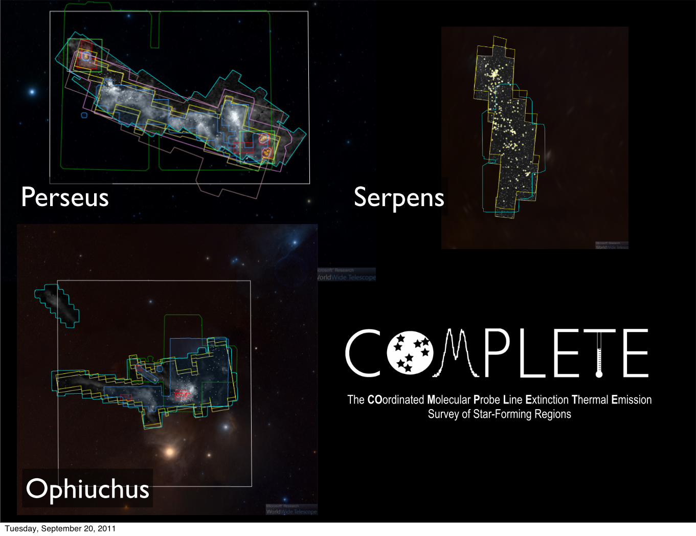
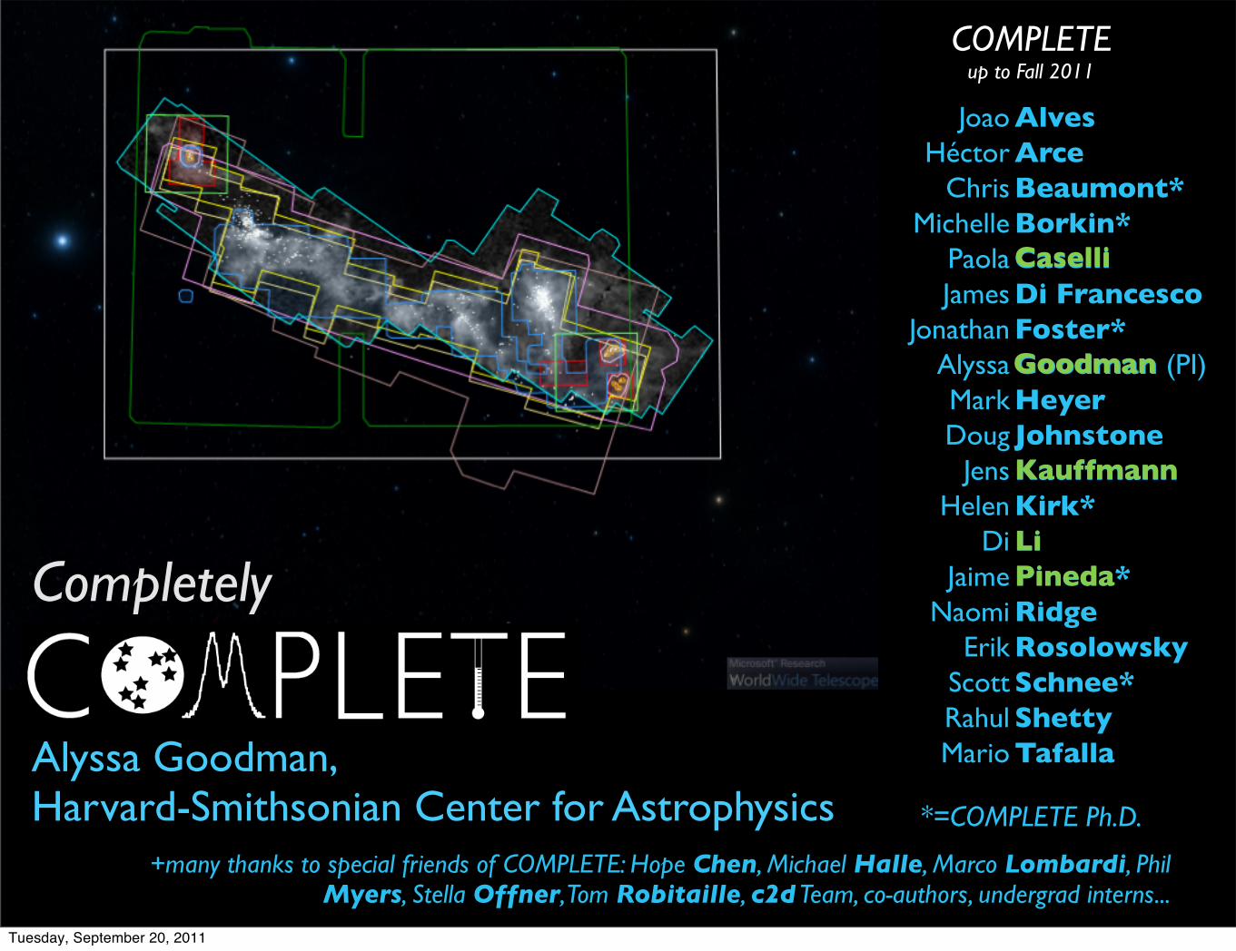
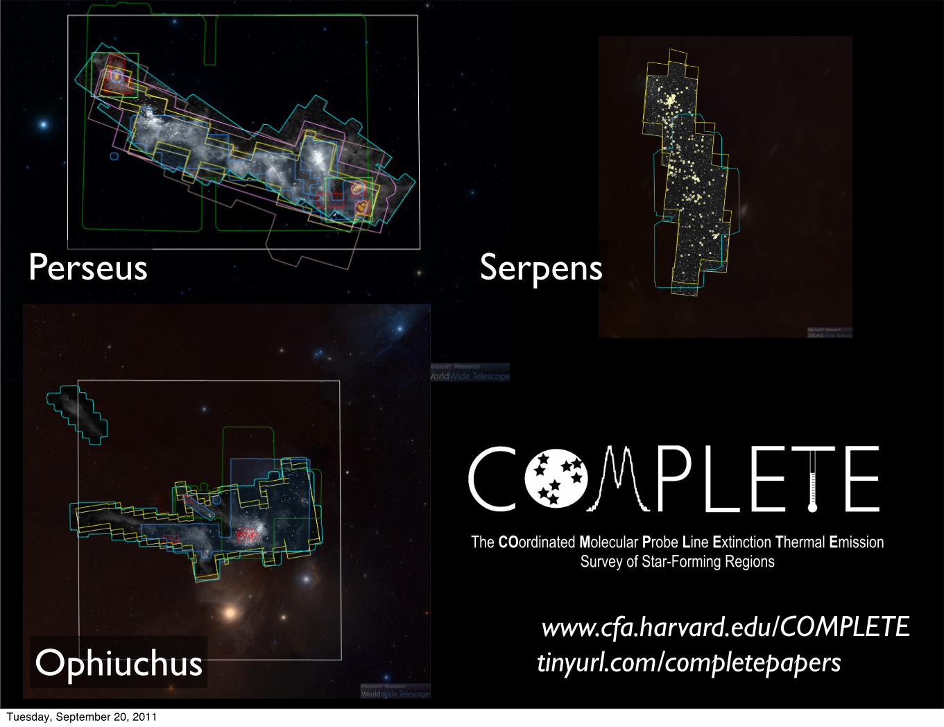
Perseus
Ophiuchus
Serpens
The COordinated Molecular Probe Line Extinction Thermal Emission Survey of Star-Forming Regions
Tuesday, September 20, 2011
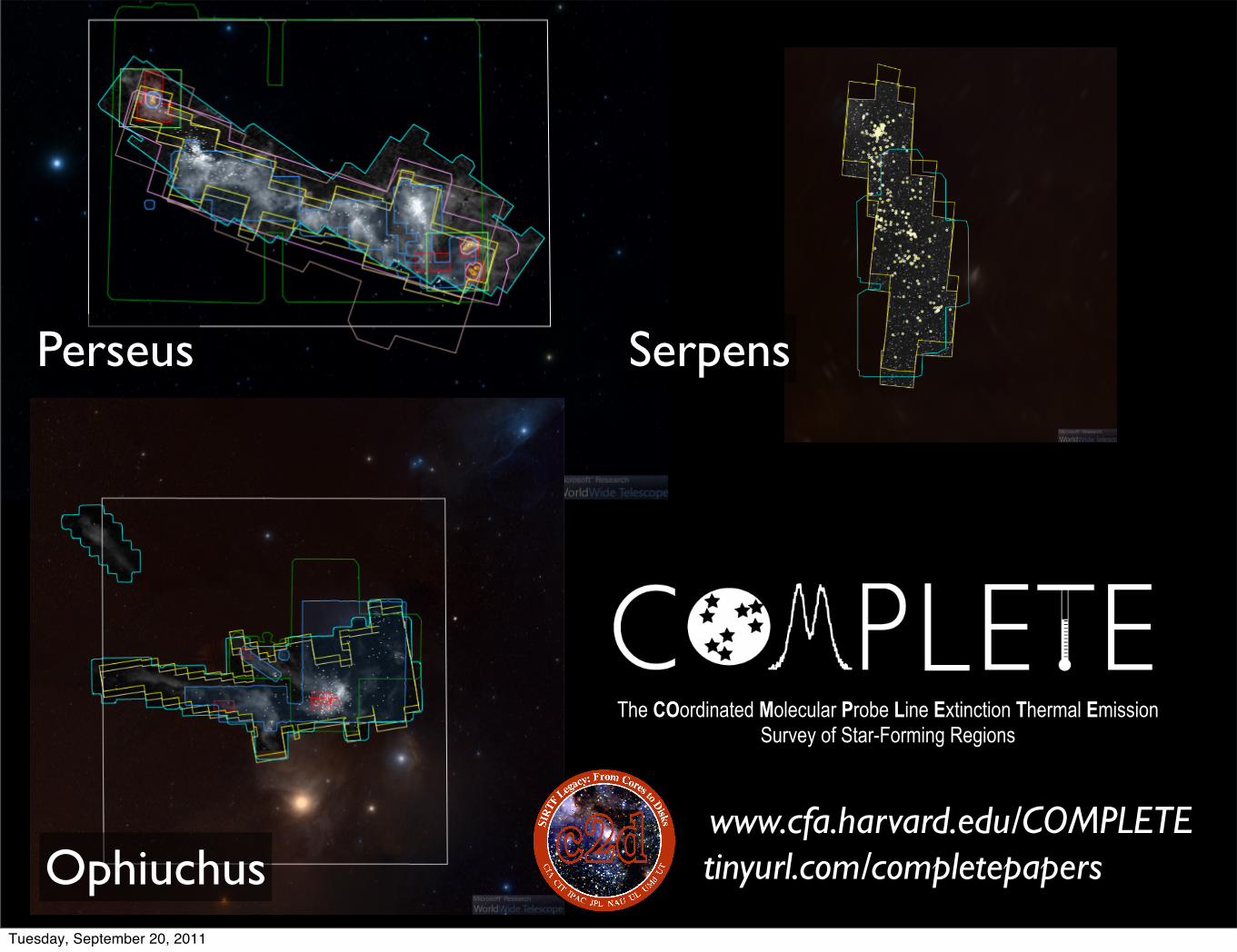
Perseus
Ophiuchus
Serpens
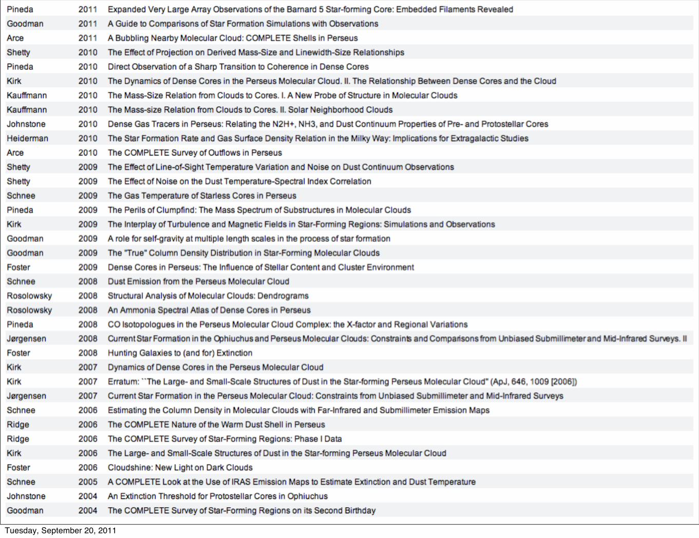
www.cfa.harvard.edu/COMPLETE
The COordinated Molecular Probe Line Extinction Thermal Emission Survey of Star-Forming Regions
tinyurl.com/completepapers
Tuesday, September 20, 2011
Perseus
Ophiuchus
Serpens
www.cfa.harvard.edu/COMPLETE
The COordinated Molecular Probe Line Extinction Thermal Emission Survey of Star-Forming Regions
tinyurl.com/completepapers
Tuesday, September 20, 2011

Perseus
Ophiuchus
Serpens
www.cfa.harvard.edu/COMPLETE
The COordinated Molecular Probe Line Extinction Thermal Emission Survey of Star-Forming Regions
tinyurl.com/completepapers
Tuesday, September 20, 2011
The “COordinated Molecular Probe Line
Extinction Thermal Emission”
Survey of Star-Forming Regions
Tuesday, September 20, 2011
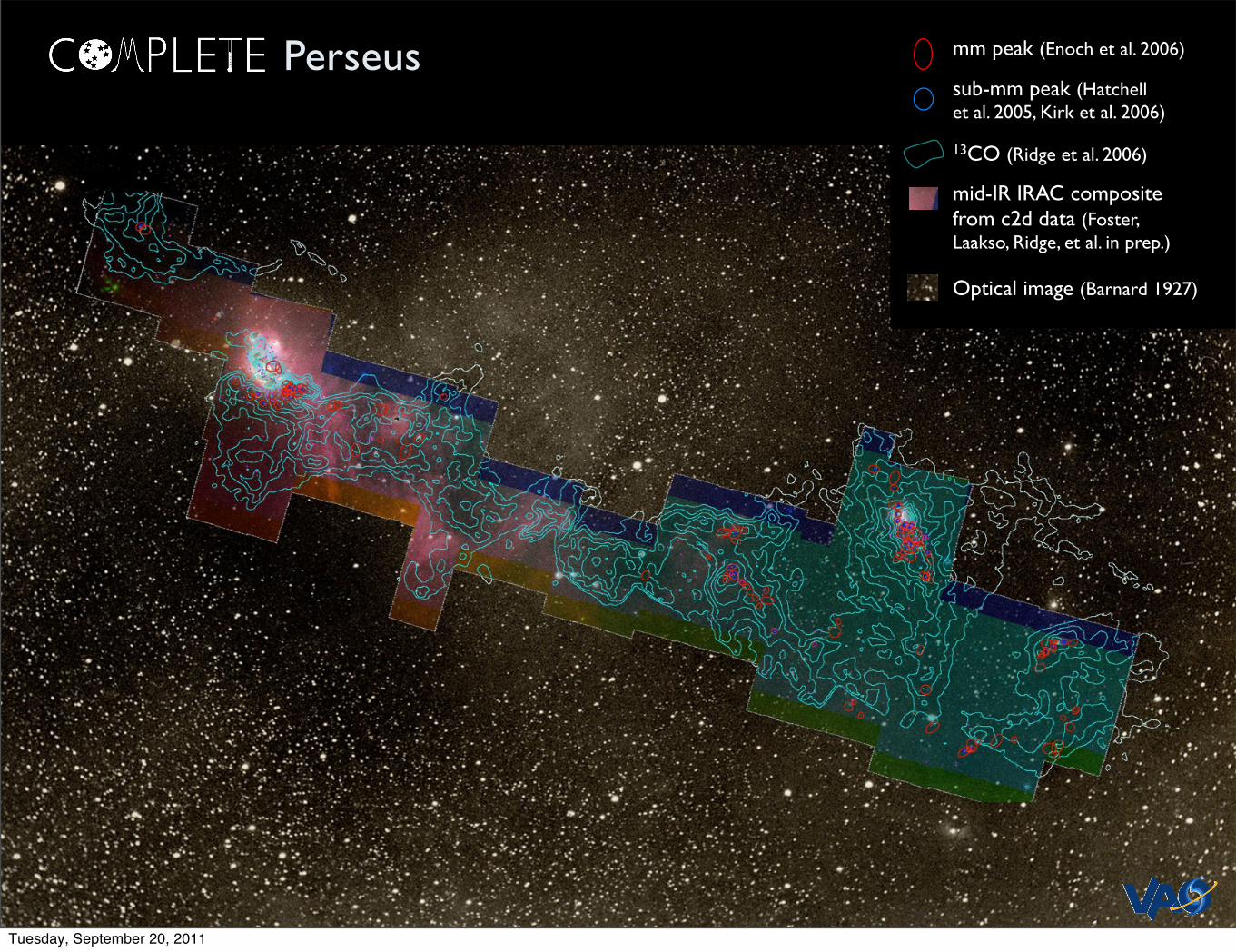
mm peak (Enoch et al. 2006)
sub-mm peak (Hatchellet al. 2005, Kirk et al. 2006)
13CO (Ridge et al. 2006)
mid-IR IRAC composite from c2d data (Foster, Laakso, Ridge, et al. in prep.)
Optical image (Barnard 1927)
Perseus
Tuesday, September 20, 2011

mm peak (Enoch et al. 2006)
sub-mm peak (Hatchellet al. 2005, Kirk et al. 2006)
13CO (Ridge et al. 2006)
mid-IR IRAC composite from c2d data (Foster, Laakso, Ridge, et al. in prep.)
Optical image (Barnard 1927)
Perseus
Tuesday, September 20, 2011

mm peak (Enoch et al. 2006)
sub-mm peak (Hatchellet al. 2005, Kirk et al. 2006)
13CO (Ridge et al. 2006)
mid-IR IRAC composite from c2d data (Foster, Laakso, Ridge, et al. in prep.)
Optical image (Barnard 1927)
Perseus
Tuesday, September 20, 2011
Tuesday, September 20, 2011
I will not do this to you...
Tuesday, September 20, 2011
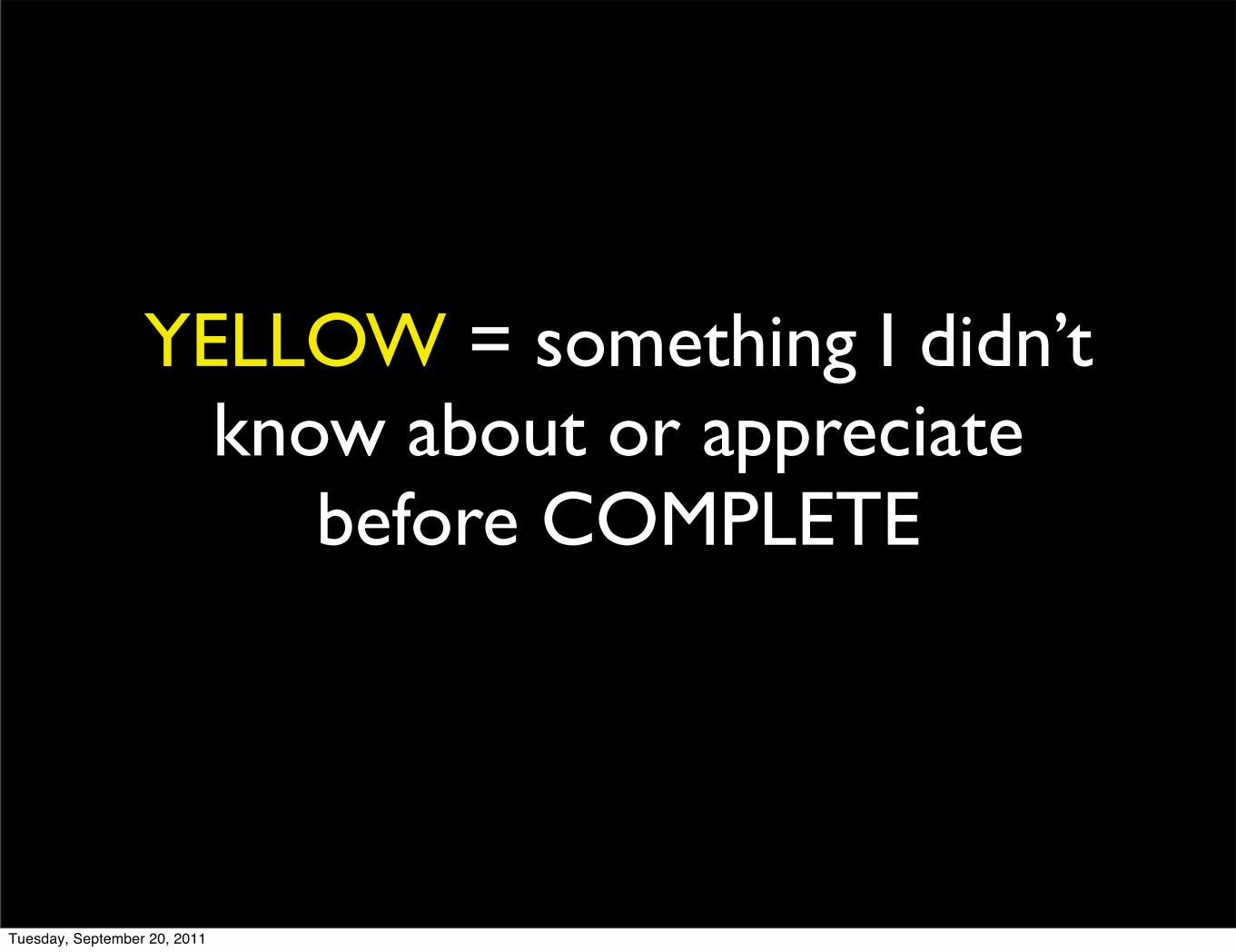
YELLOW = something I didn’t know about or appreciate
before COMPLETE
Tuesday, September 20, 2011
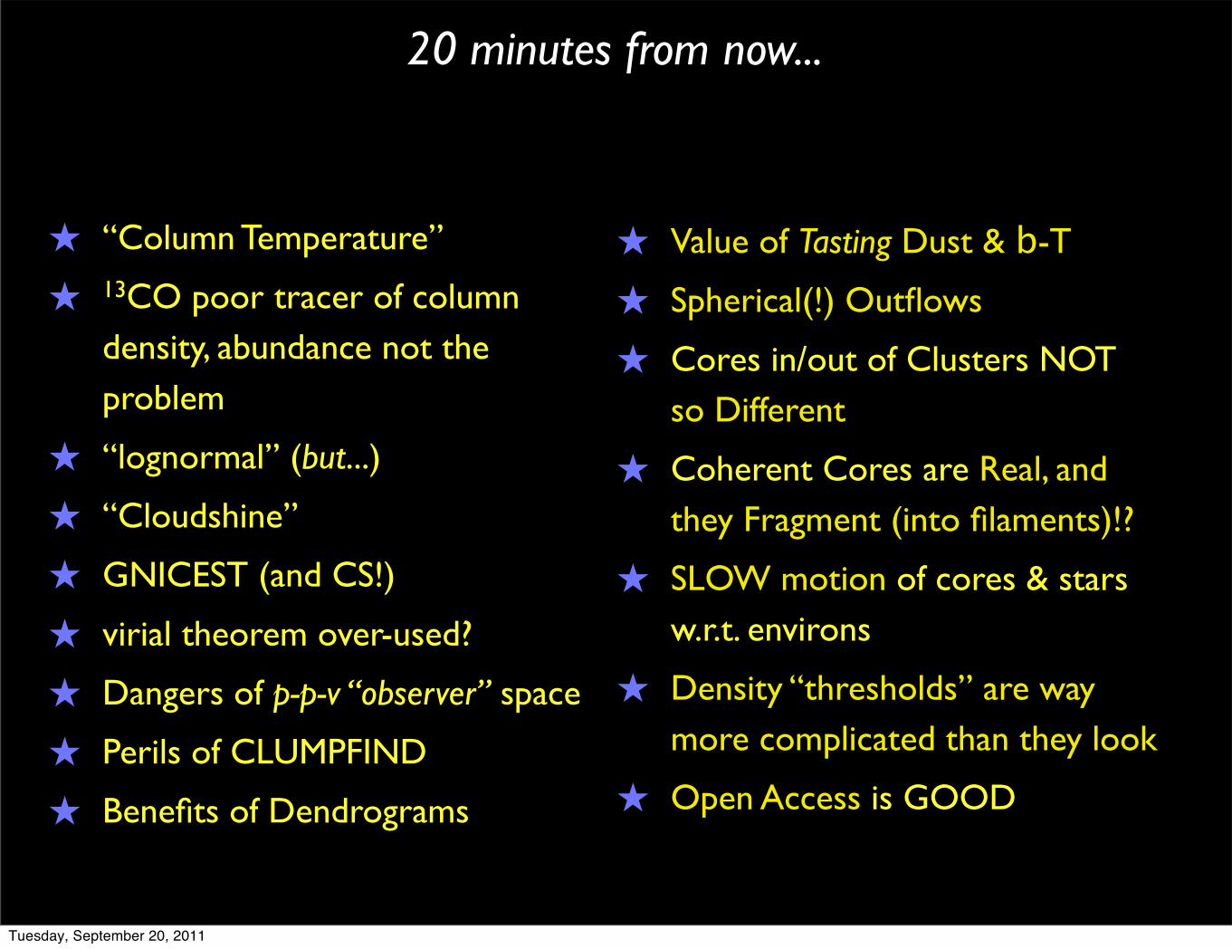
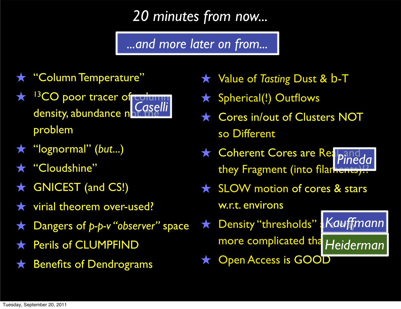
20 minutes from now...
★ “Column Temperature”
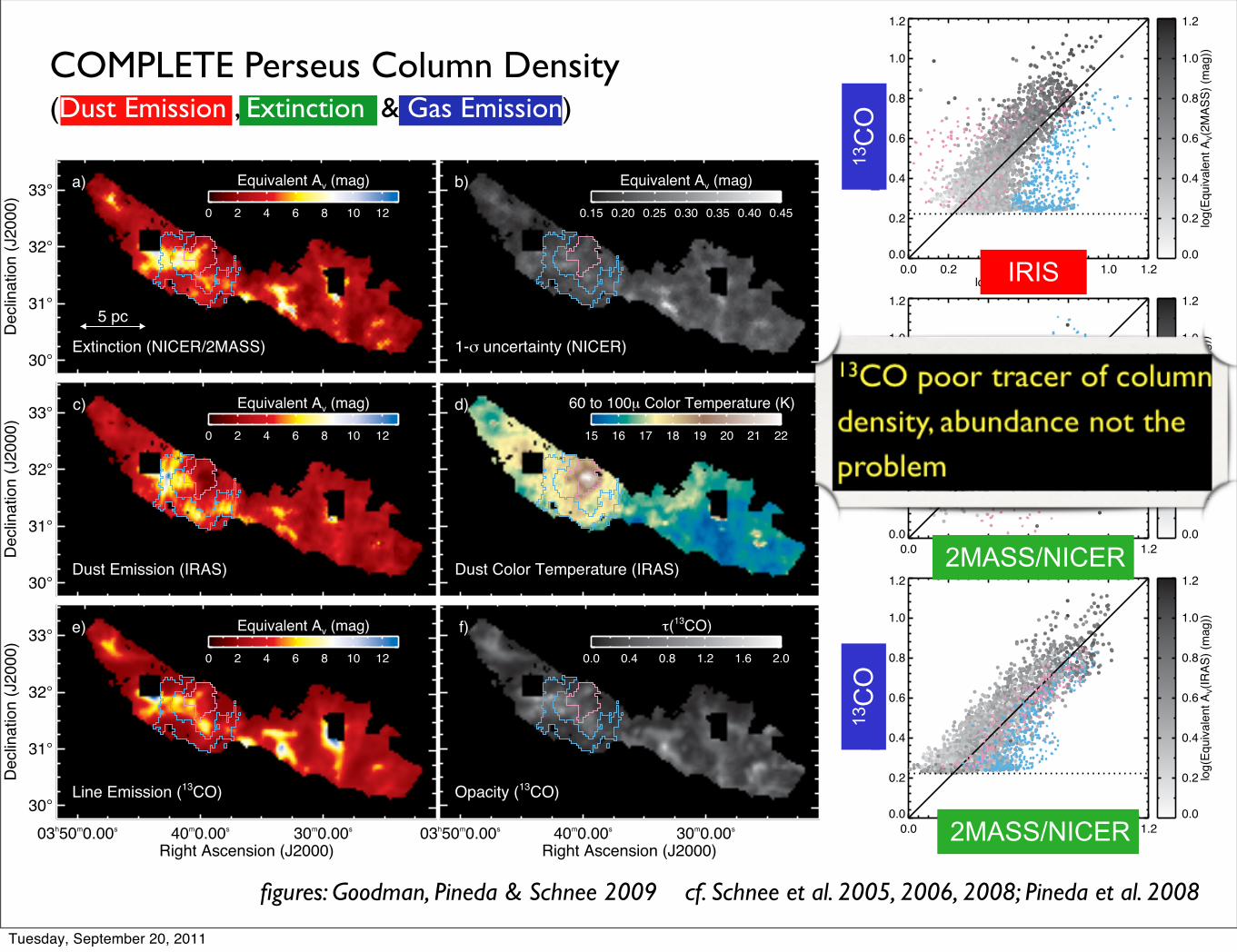
★ 13CO poor tracer of column density, abundance not the problem
★ “lognormal” (but...)
★ “Cloudshine”
★ GNICEST (and CS!)
★ virial theorem over-used?
★ Dangers of p-p-v “observer” space
★ Perils of CLUMPFIND
★ Benefits of Dendrograms
★ Value of Tasting Dust & b-T
★ Spherical(!) Outflows
★ Cores in/out of Clusters NOT so Different
★ Coherent Cores are Real, and they Fragment (into filaments)!?
★ SLOW motion of cores & stars w.r.t. environs
★ Density “thresholds” are way more complicated than they look
★ Open Access is GOOD
Tuesday, September 20, 2011

20 minutes from now...
★ “Column Temperature”
★ 13CO poor tracer of column density, abundance not the problem
★ “lognormal” (but...)
★ “Cloudshine”
★ GNICEST (and CS!)
★ virial theorem over-used?
★ Dangers of p-p-v “observer” space
★ Perils of CLUMPFIND
★ Benefits of Dendrograms
★ Value of Tasting Dust & b-T
★ Spherical(!) Outflows
★ Cores in/out of Clusters NOT so Different
★ Coherent Cores are Real, and they Fragment (into filaments)!?
★ SLOW motion of cores & stars w.r.t. environs
★ Density “thresholds” are way more complicated than they look
★ Open Access is GOOD
Pineda
Kauffmann
Caselli
...and more later on from...
Heiderman
Tuesday, September 20, 2011
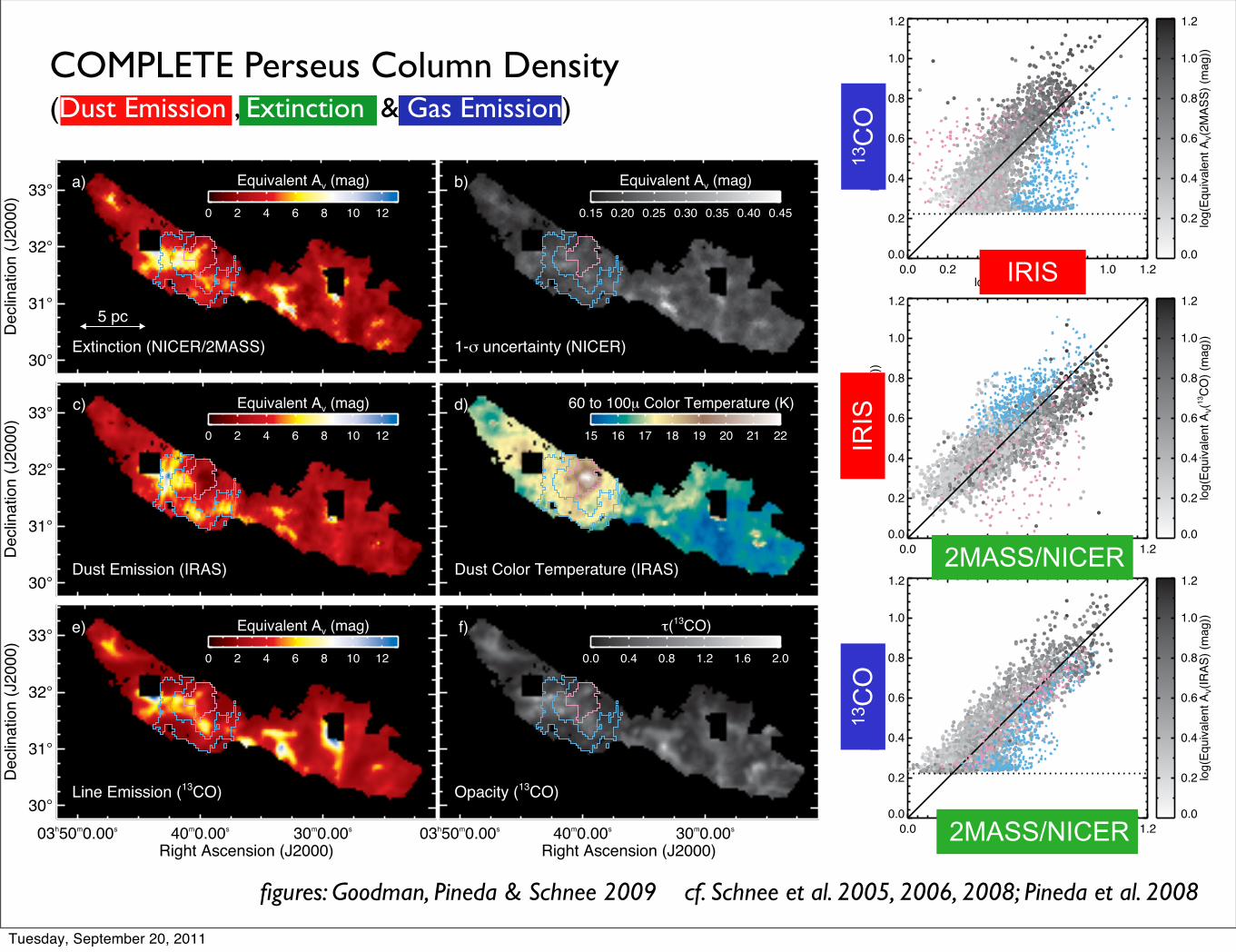
COMPLETE Perseus Column Density(Dust Emission , Extinction & Gas Emission)
Tuesday, September 20, 2011
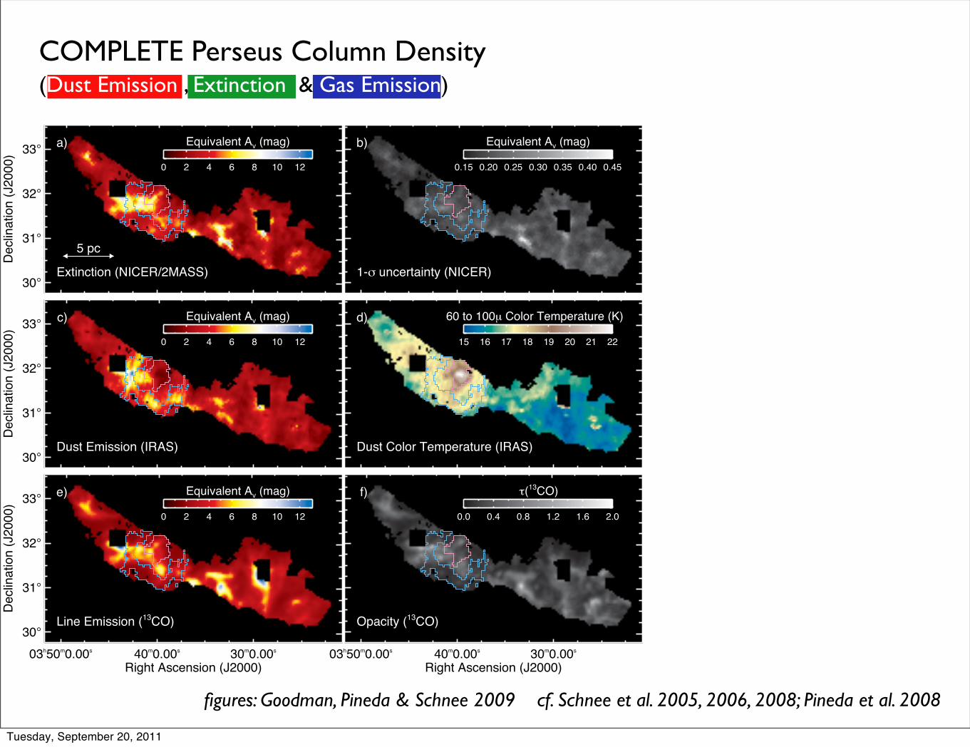
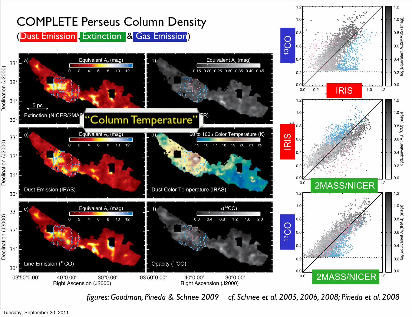
COMPLETE Perseus Column Density(Dust Emission , Extinction & Gas Emission)
Equivalent Av (mag)
2 4 6 8 10 120
5 pc
a)
Extinction (NICER/2MASS)30°
31°
32°
33°
Decli
natio
n (J
2000
)
Equivalent Av (mag)
0.15 0.20 0.25 0.30 0.35 0.40 0.45
b)
1- uncertainty (NICER)
Equivalent Av (mag)
2 4 6 8 10 120
c)
Dust Emission (IRAS)30°
31°
32°
33°
Decli
natio
n (J
2000
)
60 to 100 Color Temperature (K)
15 16 17 18 19 20 21 22
d)
Dust Color Temperature (IRAS)
Equivalent Av (mag)
2 4 6 8 10 120
e)
Line Emission (13CO)
03h50m0.00s 40m0.00s 30m0.00s
Right Ascension (J2000)
30°
31°
32°
33°
Decli
natio
n (J
2000
)
(13CO)
0.0 0.4 0.8 1.2 1.6 2.0
f)
Opacity (13CO)
03h50m0.00s 40m0.00s 30m0.00s
Right Ascension (J2000)
figures: Goodman, Pineda & Schnee 2009 cf. Schnee et al. 2005, 2006, 2008; Pineda et al. 2008
Tuesday, September 20, 2011

COMPLETE Perseus Column Density(Dust Emission , Extinction & Gas Emission)
Equivalent Av (mag)
2 4 6 8 10 120
5 pc
a)
Extinction (NICER/2MASS)30°
31°
32°
33°
Decli
natio
n (J
2000
)
Equivalent Av (mag)
0.15 0.20 0.25 0.30 0.35 0.40 0.45
b)
1- uncertainty (NICER)
Equivalent Av (mag)
2 4 6 8 10 120
c)
Dust Emission (IRAS)30°
31°
32°
33°
Decli
natio
n (J
2000
)
60 to 100 Color Temperature (K)
15 16 17 18 19 20 21 22
d)
Dust Color Temperature (IRAS)
Equivalent Av (mag)
2 4 6 8 10 120
e)
Line Emission (13CO)
03h50m0.00s 40m0.00s 30m0.00s
Right Ascension (J2000)
30°
31°
32°
33°
Decli
natio
n (J
2000
)
(13CO)
0.0 0.4 0.8 1.2 1.6 2.0
f)
Opacity (13CO)
03h50m0.00s 40m0.00s 30m0.00s
Right Ascension (J2000)
figures: Goodman, Pineda & Schnee 2009 cf. Schnee et al. 2005, 2006, 2008; Pineda et al. 2008
0.0 0.2 0.4 0.6 0.8 1.0 1.2log(AV(IRAS) (mag))
0.0
0.2
0.4
0.6
0.8
1.0
1.2
log(
A V(13
CO) (
mag
))
0.0
0.2
0.4
0.6
0.8
1.0
1.2
log(
Equi
vale
nt A
V(2M
ASS)
(mag
))
0.0 0.2 0.4 0.6 0.8 1.0 1.2log(AV(2MASS) (mag))
0.0
0.2
0.4
0.6
0.8
1.0
1.2
log(
A V(IR
AS) (
mag
))
0.0
0.2
0.4
0.6
0.8
1.0
1.2
log(
Equi
vale
nt A
V(13
CO) (
mag
))
0.0 0.2 0.4 0.6 0.8 1.0 1.2log(AV(2MASS) (mag))
0.0
0.2
0.4
0.6
0.8
1.0
1.2
log(
A V(13
CO) (
mag
))
0.0
0.2
0.4
0.6
0.8
1.0
1.2
log(
Equi
vale
nt A
V(IR
AS) (
mag
))
2MASS/NICER
IRIS
13C
O13
CO
IRIS
2MASS/NICER
Tuesday, September 20, 2011
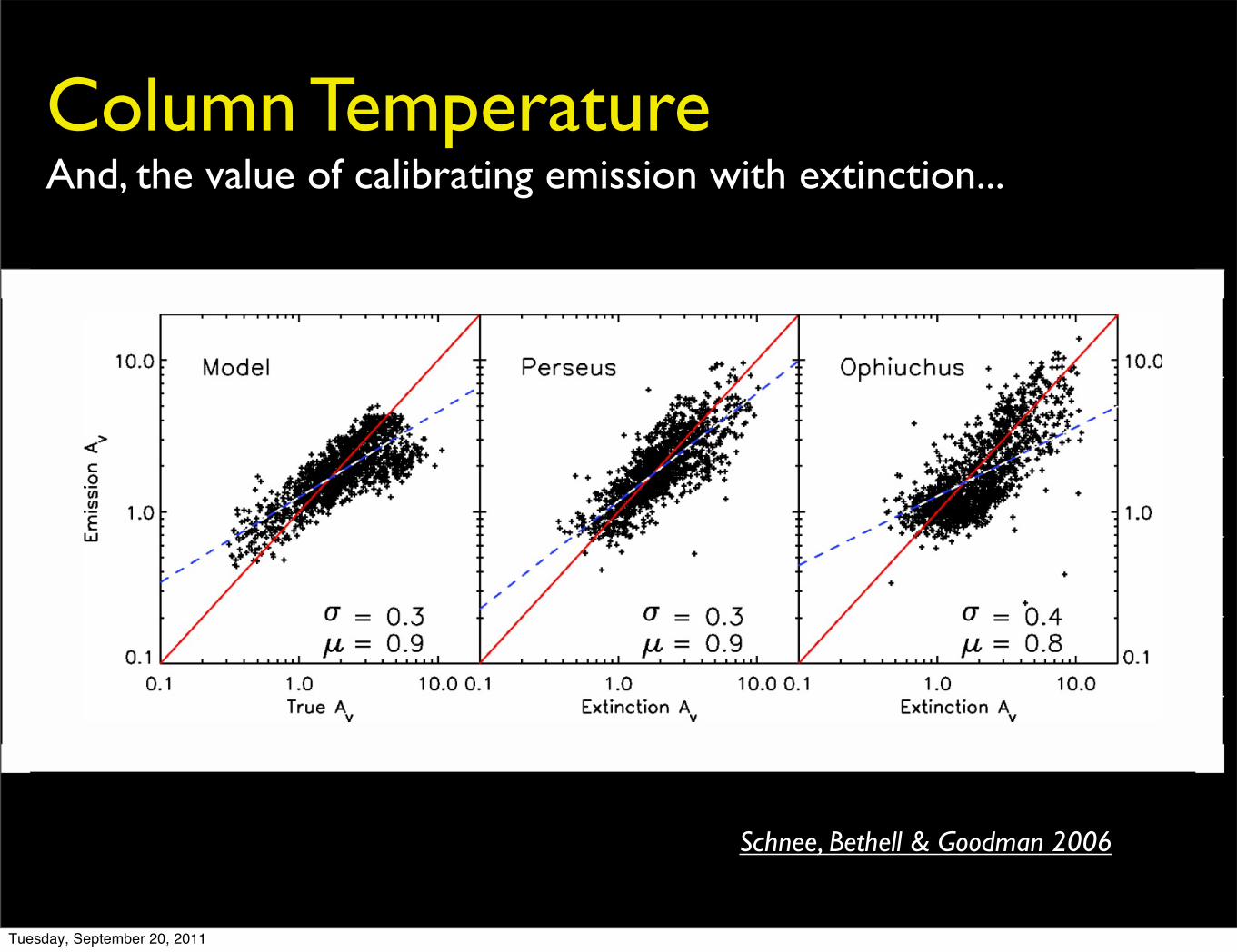
Column TemperatureAnd, the value of calibrating emission with extinction...
Schnee, Bethell & Goodman 2006
Tuesday, September 20, 2011
COMPLETE Perseus Column Density(Dust Emission , Extinction & Gas Emission)
Equivalent Av (mag)
2 4 6 8 10 120
5 pc
a)
Extinction (NICER/2MASS)30°
31°
32°
33°
Decli
natio
n (J
2000
)
Equivalent Av (mag)
0.15 0.20 0.25 0.30 0.35 0.40 0.45
b)
1- uncertainty (NICER)
Equivalent Av (mag)
2 4 6 8 10 120
c)
Dust Emission (IRAS)30°
31°
32°
33°
Decli
natio
n (J
2000
)
60 to 100 Color Temperature (K)
15 16 17 18 19 20 21 22
d)
Dust Color Temperature (IRAS)
Equivalent Av (mag)
2 4 6 8 10 120
e)
Line Emission (13CO)
03h50m0.00s 40m0.00s 30m0.00s
Right Ascension (J2000)
30°
31°
32°
33°
Decli
natio
n (J
2000
)
(13CO)
0.0 0.4 0.8 1.2 1.6 2.0
f)
Opacity (13CO)
03h50m0.00s 40m0.00s 30m0.00s
Right Ascension (J2000)
figures: Goodman, Pineda & Schnee 2009 cf. Schnee et al. 2005, 2006, 2008; Pineda et al. 2008
0.0 0.2 0.4 0.6 0.8 1.0 1.2log(AV(IRAS) (mag))
0.0
0.2
0.4
0.6
0.8
1.0
1.2
log(
A V(13
CO) (
mag
))
0.0
0.2
0.4
0.6
0.8
1.0
1.2
log(
Equi
vale
nt A
V(2M
ASS)
(mag
))
0.0 0.2 0.4 0.6 0.8 1.0 1.2log(AV(2MASS) (mag))
0.0
0.2
0.4
0.6
0.8
1.0
1.2
log(
A V(IR
AS) (
mag
))
0.0
0.2
0.4
0.6
0.8
1.0
1.2
log(
Equi
vale
nt A
V(13
CO) (
mag
))
0.0 0.2 0.4 0.6 0.8 1.0 1.2log(AV(2MASS) (mag))
0.0
0.2
0.4
0.6
0.8
1.0
1.2
log(
A V(13
CO) (
mag
))
0.0
0.2
0.4
0.6
0.8
1.0
1.2
log(
Equi
vale
nt A
V(IR
AS) (
mag
))
2MASS/NICER
IRIS
13C
O13
CO
IRIS
2MASS/NICER
Tuesday, September 20, 2011
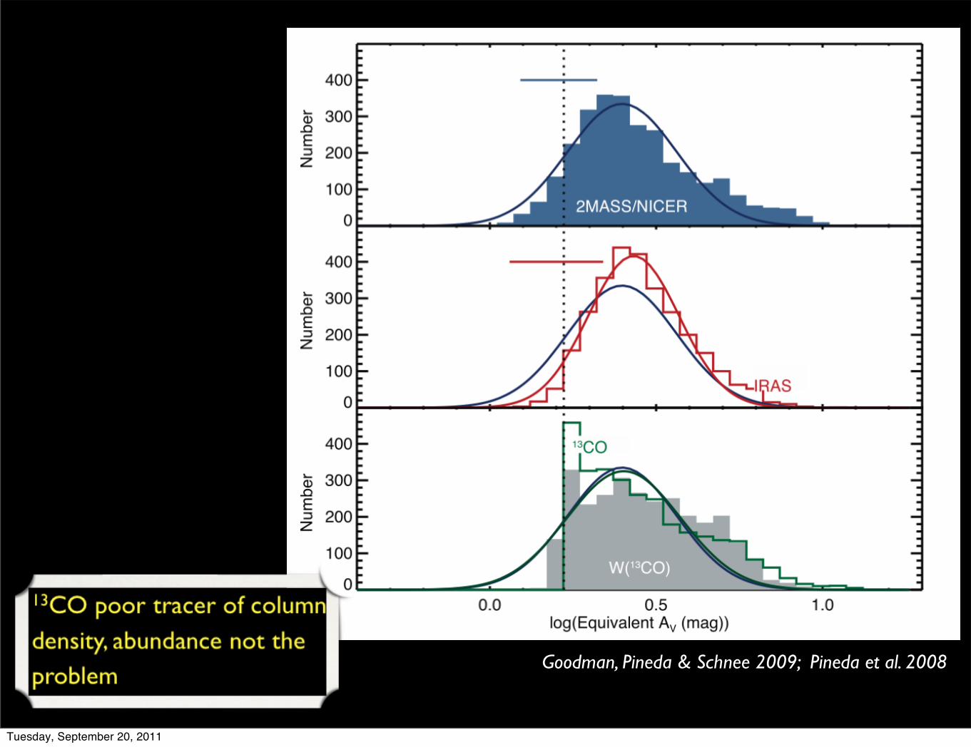
Goodman, Pineda & Schnee 2009; Pineda et al. 2008
Tuesday, September 20, 2011
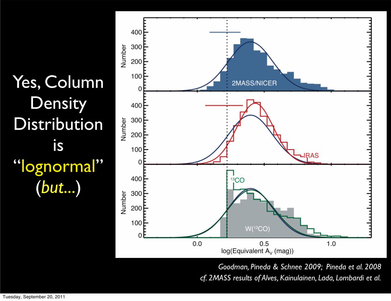
Yes, Column Density
Distribution is
“lognormal” (but...)
Goodman, Pineda & Schnee 2009; Pineda et al. 2008 cf. 2MASS results of Alves, Kainulainen, Lada, Lombardi et al.
Tuesday, September 20, 2011
...Justin Bieber, and the IMF, can be lognormal too...
see Beaumont et al. 2011, and http://www.ifa.hawaii.edu/users/beaumont/histograms/index.html
and so is any multiplicative random process.
Tuesday, September 20, 2011
...Justin Bieber, and the IMF, can be lognormal too...
see Beaumont et al. 2011, and http://www.ifa.hawaii.edu/users/beaumont/histograms/index.html
and so is any multiplicative random process.
Tuesday, September 20, 2011
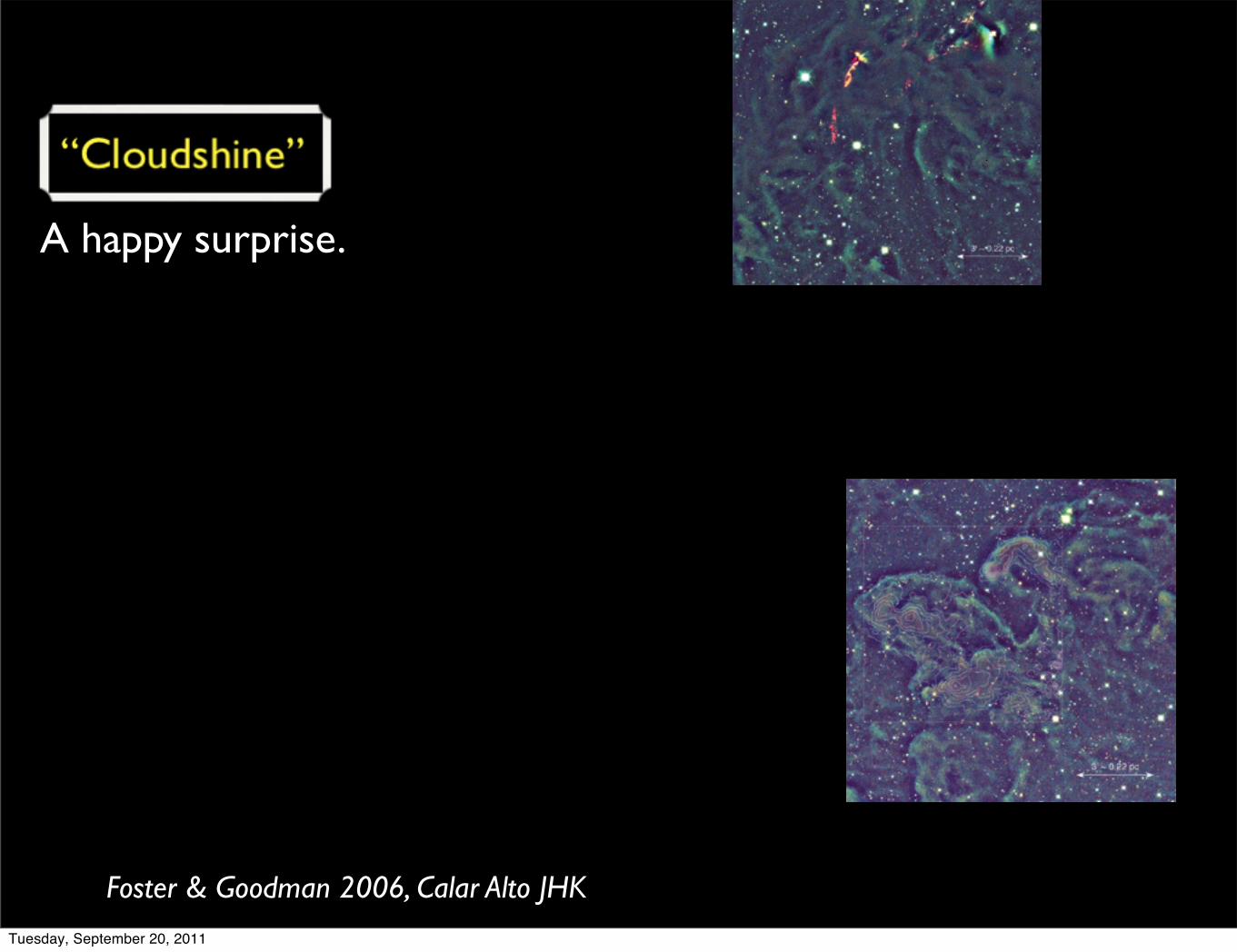
A happy surprise.
Tuesday, September 20, 2011
A happy surprise.
Foster & Goodman 2006, Calar Alto JHK
Tuesday, September 20, 2011
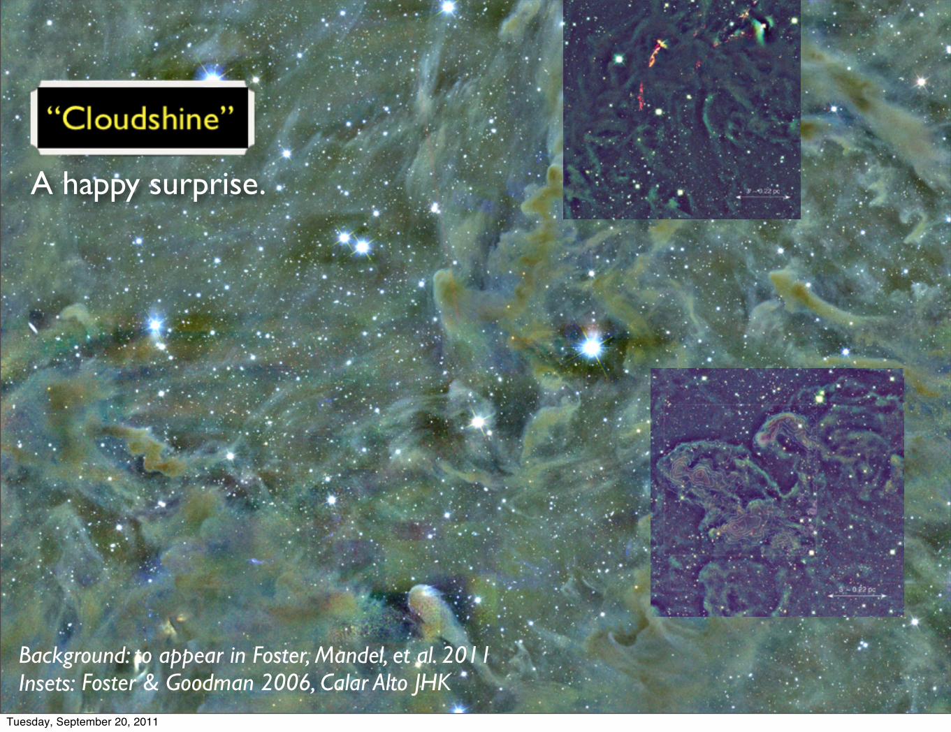
Background: to appear in Foster, Mandel, et al. 2011Insets:
A happy surprise.
Foster & Goodman 2006, Calar Alto JHK
Tuesday, September 20, 2011

Background: to appear in Foster, Mandel, et al. 2011Insets:
A happy surprise.
Foster & Goodman 2006, Calar Alto JHK
Tuesday, September 20, 2011
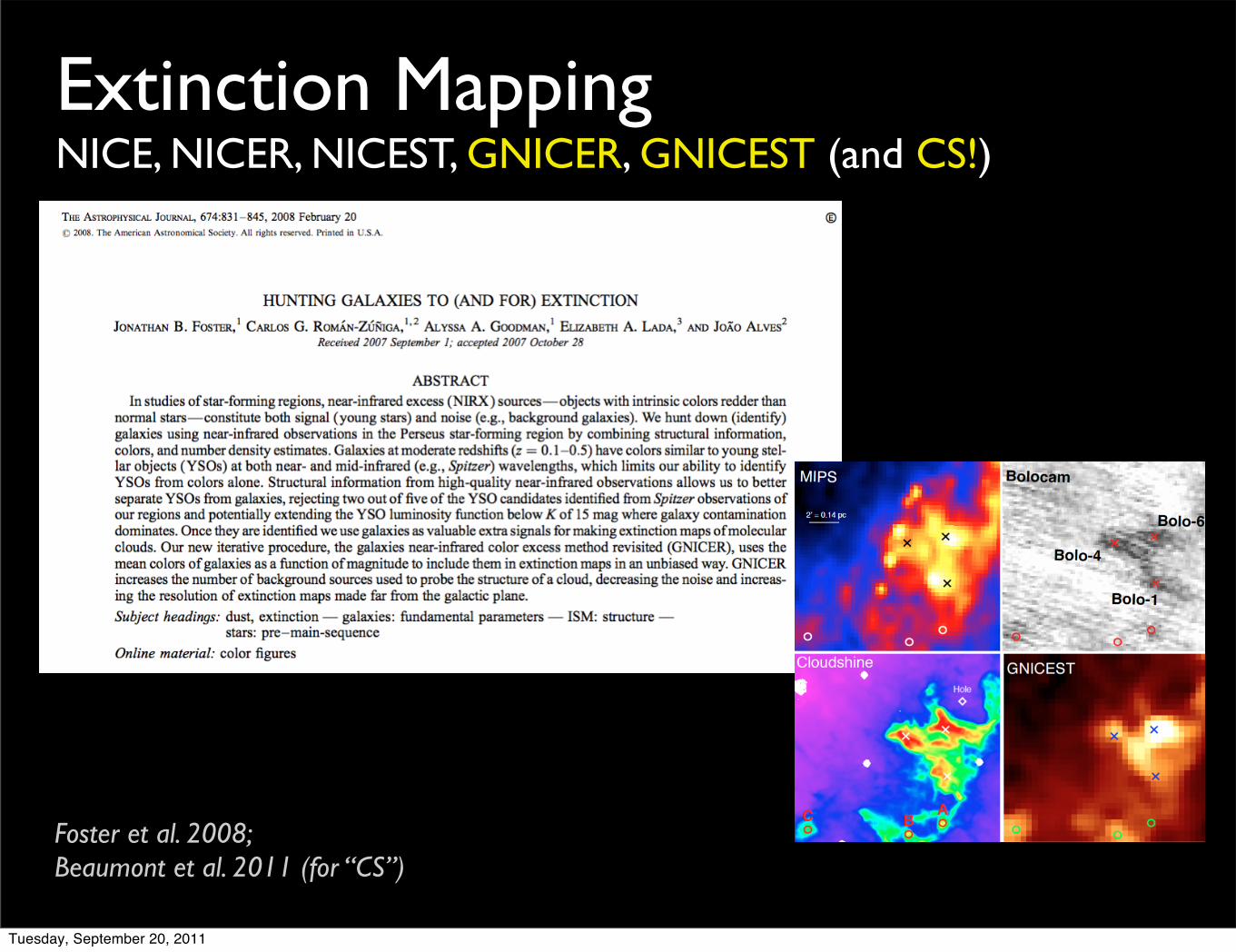
Extinction MappingNICE, NICER, NICEST, GNICER, GNICEST (and CS!)
Foster et al. 2008; Beaumont et al. 2011 (for “CS”)
Tuesday, September 20, 2011
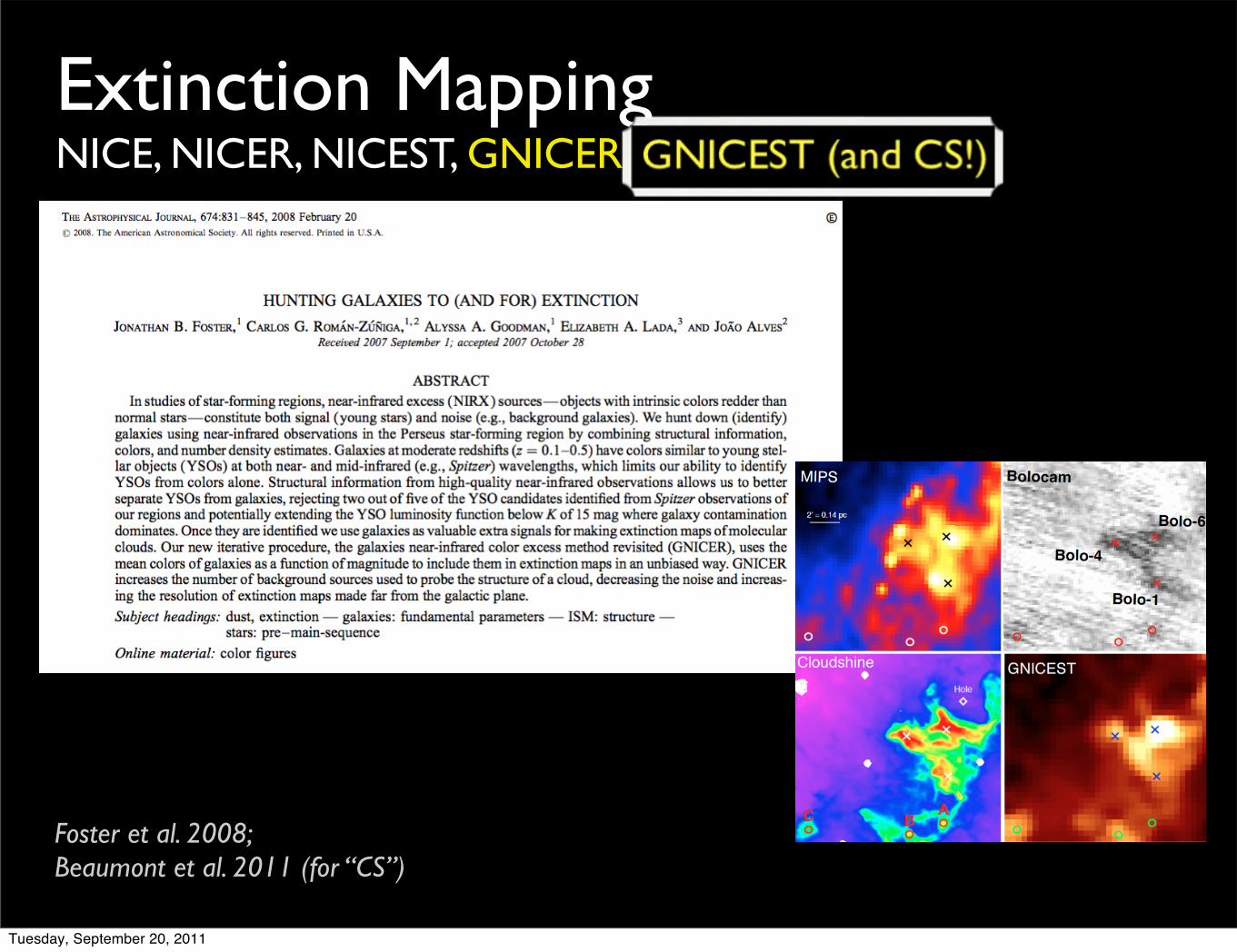
Extinction MappingNICE, NICER, NICEST, GNICER, GNICEST (and CS!)
Foster et al. 2008; Beaumont et al. 2011 (for “CS”)
Tuesday, September 20, 2011

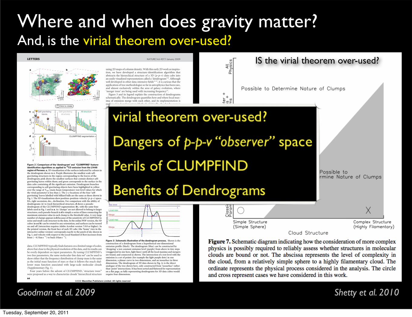
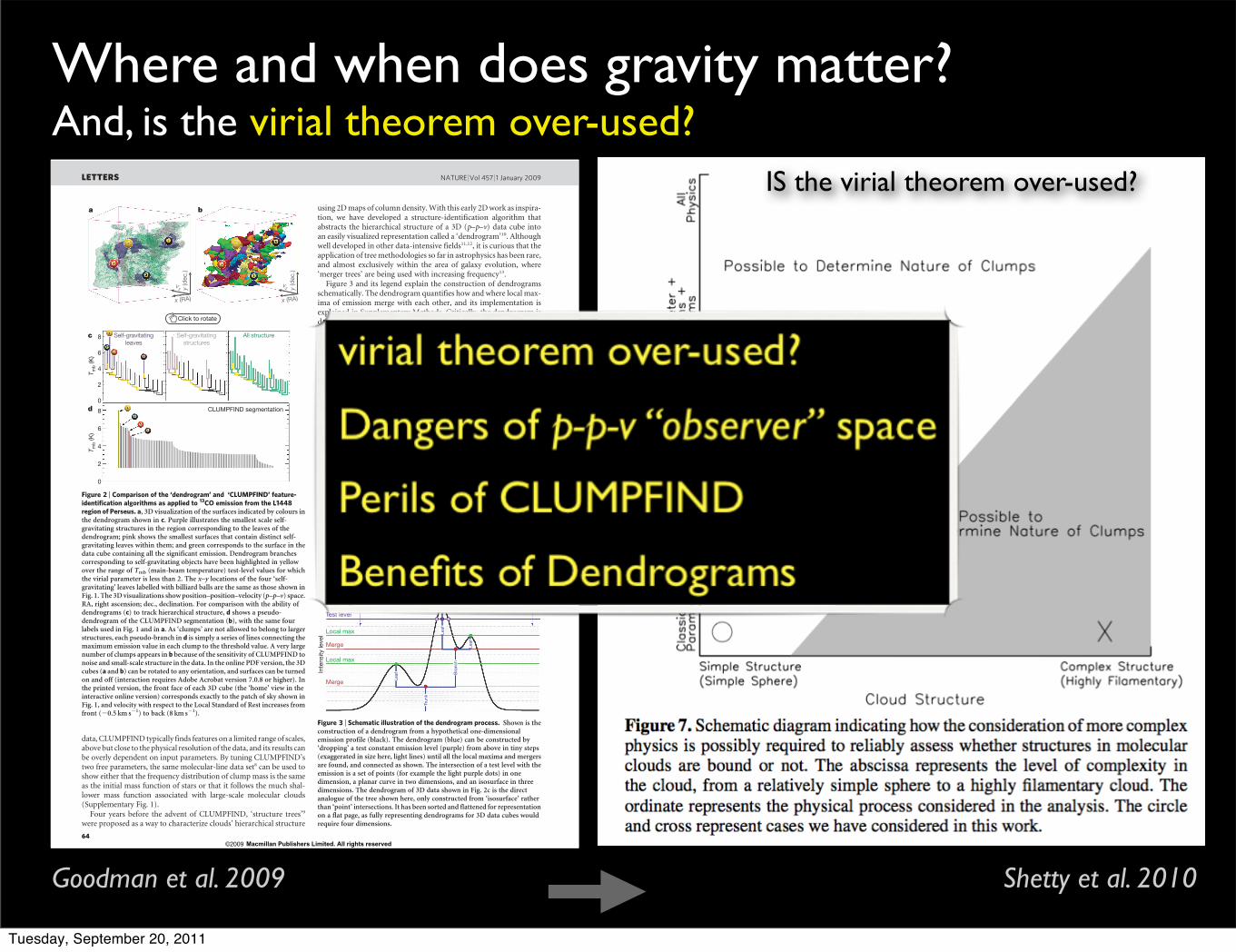
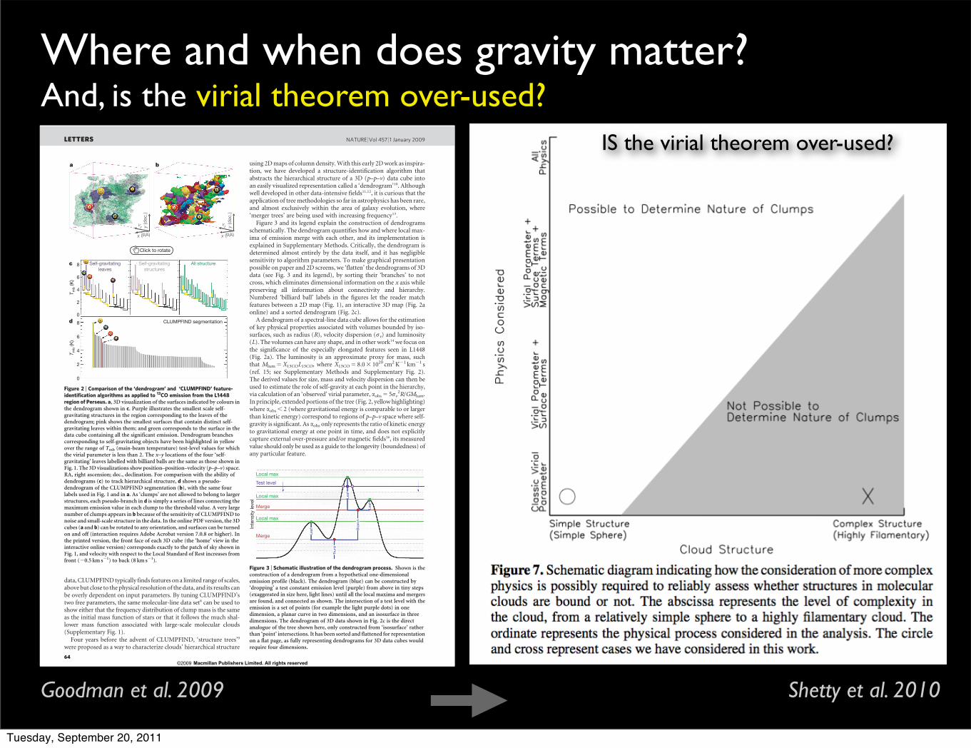
Where and when does gravity matter?And, is the virial theorem over-used?
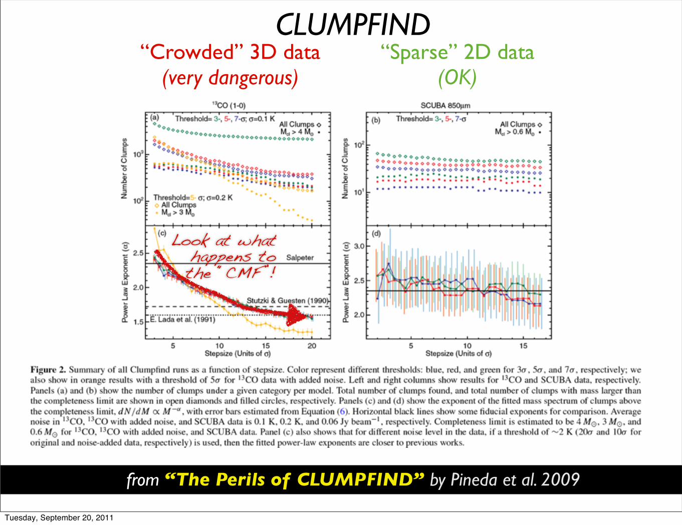
data, CLUMPFIND typically finds features on a limited range of scales,abovebut close to thephysical resolution of thedata, and its results canbe overly dependent on input parameters. By tuning CLUMPFIND’stwo free parameters, the same molecular-line data set8 can be used toshow either that the frequency distribution of clumpmass is the sameas the initial mass function of stars or that it follows the much shal-lower mass function associated with large-scale molecular clouds(Supplementary Fig. 1).
Four years before the advent of CLUMPFIND, ‘structure trees’9
were proposed as a way to characterize clouds’ hierarchical structure
using 2Dmaps of column density.With this early 2Dwork as inspira-tion, we have developed a structure-identification algorithm thatabstracts the hierarchical structure of a 3D (p–p–v) data cube intoan easily visualized representation called a ‘dendrogram’10. Althoughwell developed in other data-intensive fields11,12, it is curious that theapplication of treemethodologies so far in astrophysics has been rare,and almost exclusively within the area of galaxy evolution, where‘merger trees’ are being used with increasing frequency13.
Figure 3 and its legend explain the construction of dendrogramsschematically. The dendrogram quantifies how and where local max-ima of emission merge with each other, and its implementation isexplained in Supplementary Methods. Critically, the dendrogram isdetermined almost entirely by the data itself, and it has negligiblesensitivity to algorithm parameters. To make graphical presentationpossible on paper and 2D screens, we ‘flatten’ the dendrograms of 3Ddata (see Fig. 3 and its legend), by sorting their ‘branches’ to notcross, which eliminates dimensional information on the x axis whilepreserving all information about connectivity and hierarchy.Numbered ‘billiard ball’ labels in the figures let the reader matchfeatures between a 2D map (Fig. 1), an interactive 3D map (Fig. 2aonline) and a sorted dendrogram (Fig. 2c).
A dendrogramof a spectral-line data cube allows for the estimationof key physical properties associated with volumes bounded by iso-surfaces, such as radius (R), velocity dispersion (sv) and luminosity(L). The volumes can have any shape, and in other work14 we focus onthe significance of the especially elongated features seen in L1448(Fig. 2a). The luminosity is an approximate proxy for mass, suchthat Mlum5X13COL13CO, where X13CO5 8.03 1020 cm2K21 km21 s(ref. 15; see Supplementary Methods and Supplementary Fig. 2).The derived values for size, mass and velocity dispersion can then beused to estimate the role of self-gravity at each point in the hierarchy,via calculation of an ‘observed’ virial parameter, aobs5 5sv
2R/GMlum.In principle, extended portions of the tree (Fig. 2, yellow highlighting)where aobs, 2 (where gravitational energy is comparable to or largerthan kinetic energy) correspond to regions of p–p–v space where self-gravity is significant. As aobs only represents the ratio of kinetic energyto gravitational energy at one point in time, and does not explicitlycapture external over-pressure and/or magnetic fields16, its measuredvalue should only be used as a guide to the longevity (boundedness) ofany particular feature.
Self-gravitatingleaves
CLUMPFIND segmentation
vz
x (RA)
y (d
ec.)
vz
x (RA) y
(dec
.)
c
d
8
6
4
2
0
8
6
4
2
0
T mb
(K)
T mb
(K)
Self-gravitatingstructures
All structure
a b
Click to rotate
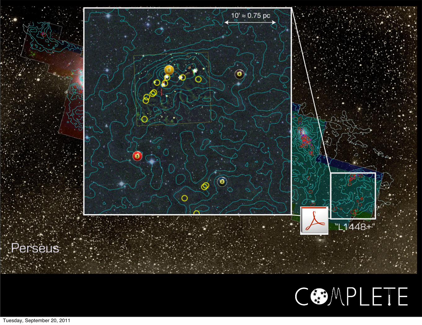
Figure 2 | Comparison of the ‘dendrogram’ and ‘CLUMPFIND’ feature-identification algorithms as applied to 13CO emission from the L1448region of Perseus. a, 3D visualization of the surfaces indicated by colours inthe dendrogram shown in c. Purple illustrates the smallest scale self-gravitating structures in the region corresponding to the leaves of thedendrogram; pink shows the smallest surfaces that contain distinct self-gravitating leaves within them; and green corresponds to the surface in thedata cube containing all the significant emission. Dendrogram branchescorresponding to self-gravitating objects have been highlighted in yellowover the range of Tmb (main-beam temperature) test-level values for whichthe virial parameter is less than 2. The x–y locations of the four ‘self-gravitating’ leaves labelled with billiard balls are the same as those shown inFig. 1. The 3D visualizations showposition–position–velocity (p–p–v) space.RA, right ascension; dec., declination. For comparison with the ability ofdendrograms (c) to track hierarchical structure, d shows a pseudo-dendrogram of the CLUMPFIND segmentation (b), with the same fourlabels used in Fig. 1 and in a. As ‘clumps’ are not allowed to belong to largerstructures, each pseudo-branch in d is simply a series of lines connecting themaximum emission value in each clump to the threshold value. A very largenumber of clumps appears in b because of the sensitivity of CLUMPFIND tonoise and small-scale structure in the data. In the online PDF version, the 3Dcubes (a and b) can be rotated to any orientation, and surfaces can be turnedon and off (interaction requires Adobe Acrobat version 7.0.8 or higher). Inthe printed version, the front face of each 3D cube (the ‘home’ view in theinteractive online version) corresponds exactly to the patch of sky shown inFig. 1, and velocity with respect to the Local Standard of Rest increases fromfront (20.5 km s21) to back (8 km s21).
Inte
nsity
leve
l
Local max
Local max
Local max
Merge
Merge
Leaf
Leaf
Leaf
Bra
nch
Trun
k
Test level
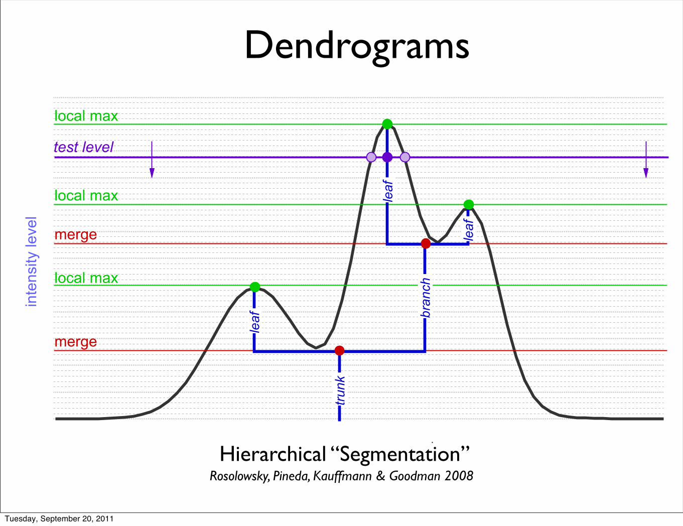
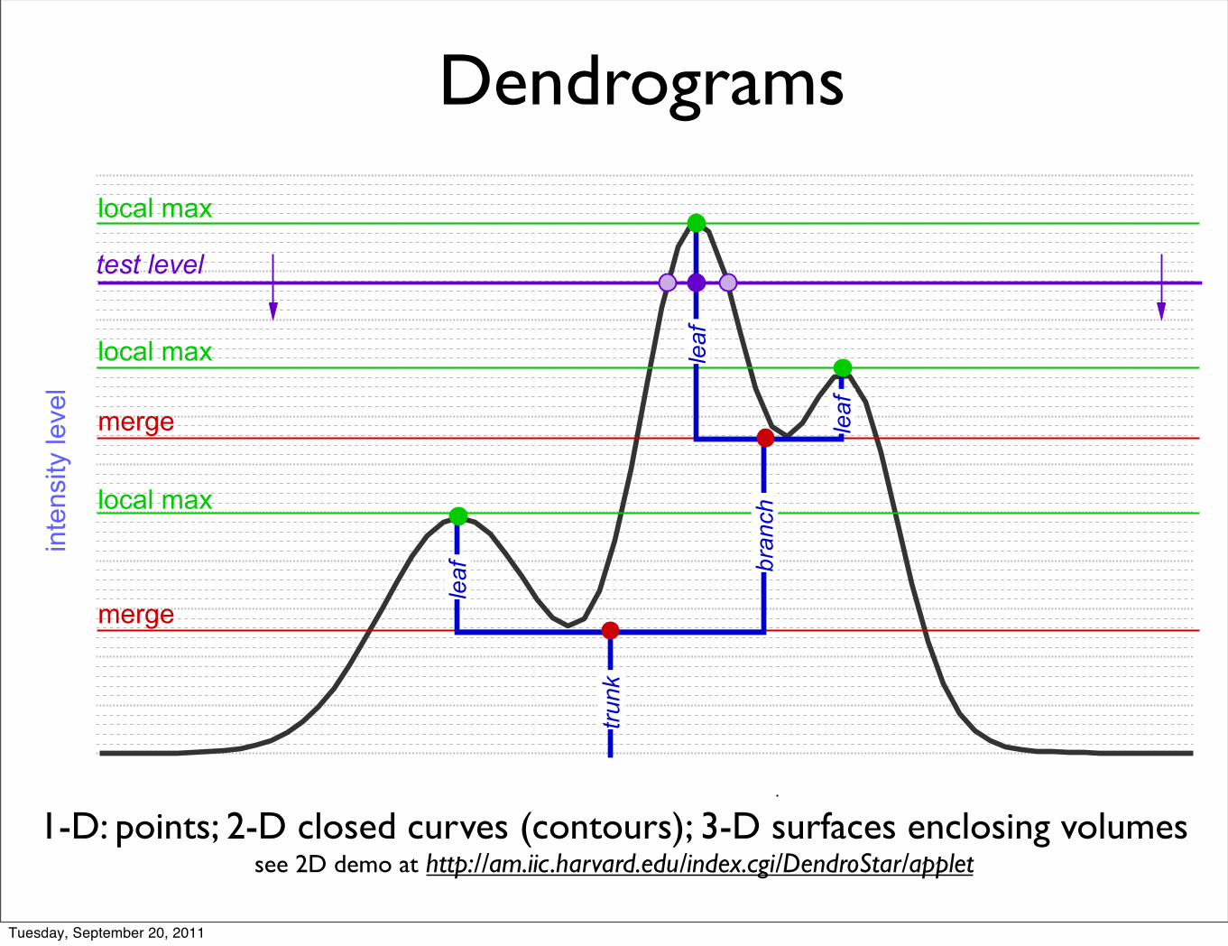
Figure 3 | Schematic illustration of the dendrogram process. Shown is theconstruction of a dendrogram from a hypothetical one-dimensionalemission profile (black). The dendrogram (blue) can be constructed by‘dropping’ a test constant emission level (purple) from above in tiny steps(exaggerated in size here, light lines) until all the local maxima and mergersare found, and connected as shown. The intersection of a test level with theemission is a set of points (for example the light purple dots) in onedimension, a planar curve in two dimensions, and an isosurface in threedimensions. The dendrogram of 3D data shown in Fig. 2c is the directanalogue of the tree shown here, only constructed from ‘isosurface’ ratherthan ‘point’ intersections. It has been sorted and flattened for representationon a flat page, as fully representing dendrograms for 3D data cubes wouldrequire four dimensions.
LETTERS NATURE |Vol 457 | 1 January 2009
64 Macmillan Publishers Limited. All rights reserved©2009
Goodman et al. 2009 Shetty et al. 2010
IS the virial theorem over-used?
Tuesday, September 20, 2011
Where and when does gravity matter?And, is the virial theorem over-used?
data, CLUMPFIND typically finds features on a limited range of scales,abovebut close to thephysical resolution of thedata, and its results canbe overly dependent on input parameters. By tuning CLUMPFIND’stwo free parameters, the same molecular-line data set8 can be used toshow either that the frequency distribution of clumpmass is the sameas the initial mass function of stars or that it follows the much shal-lower mass function associated with large-scale molecular clouds(Supplementary Fig. 1).
Four years before the advent of CLUMPFIND, ‘structure trees’9
were proposed as a way to characterize clouds’ hierarchical structure
using 2Dmaps of column density.With this early 2Dwork as inspira-tion, we have developed a structure-identification algorithm thatabstracts the hierarchical structure of a 3D (p–p–v) data cube intoan easily visualized representation called a ‘dendrogram’10. Althoughwell developed in other data-intensive fields11,12, it is curious that theapplication of treemethodologies so far in astrophysics has been rare,and almost exclusively within the area of galaxy evolution, where‘merger trees’ are being used with increasing frequency13.
Figure 3 and its legend explain the construction of dendrogramsschematically. The dendrogram quantifies how and where local max-ima of emission merge with each other, and its implementation isexplained in Supplementary Methods. Critically, the dendrogram isdetermined almost entirely by the data itself, and it has negligiblesensitivity to algorithm parameters. To make graphical presentationpossible on paper and 2D screens, we ‘flatten’ the dendrograms of 3Ddata (see Fig. 3 and its legend), by sorting their ‘branches’ to notcross, which eliminates dimensional information on the x axis whilepreserving all information about connectivity and hierarchy.Numbered ‘billiard ball’ labels in the figures let the reader matchfeatures between a 2D map (Fig. 1), an interactive 3D map (Fig. 2aonline) and a sorted dendrogram (Fig. 2c).
A dendrogramof a spectral-line data cube allows for the estimationof key physical properties associated with volumes bounded by iso-surfaces, such as radius (R), velocity dispersion (sv) and luminosity(L). The volumes can have any shape, and in other work14 we focus onthe significance of the especially elongated features seen in L1448(Fig. 2a). The luminosity is an approximate proxy for mass, suchthat Mlum5X13COL13CO, where X13CO5 8.03 1020 cm2K21 km21 s(ref. 15; see Supplementary Methods and Supplementary Fig. 2).The derived values for size, mass and velocity dispersion can then beused to estimate the role of self-gravity at each point in the hierarchy,via calculation of an ‘observed’ virial parameter, aobs5 5sv
2R/GMlum.In principle, extended portions of the tree (Fig. 2, yellow highlighting)where aobs, 2 (where gravitational energy is comparable to or largerthan kinetic energy) correspond to regions of p–p–v space where self-gravity is significant. As aobs only represents the ratio of kinetic energyto gravitational energy at one point in time, and does not explicitlycapture external over-pressure and/or magnetic fields16, its measuredvalue should only be used as a guide to the longevity (boundedness) ofany particular feature.
Self-gravitatingleaves
CLUMPFIND segmentation
vz
x (RA)
y (d
ec.)
vz
x (RA) y
(dec
.)
c
d
8
6
4
2
0
8
6
4
2
0
T mb
(K)
T mb
(K)
Self-gravitatingstructures
All structure
a b
Click to rotate
Figure 2 | Comparison of the ‘dendrogram’ and ‘CLUMPFIND’ feature-identification algorithms as applied to 13CO emission from the L1448region of Perseus. a, 3D visualization of the surfaces indicated by colours inthe dendrogram shown in c. Purple illustrates the smallest scale self-gravitating structures in the region corresponding to the leaves of thedendrogram; pink shows the smallest surfaces that contain distinct self-gravitating leaves within them; and green corresponds to the surface in thedata cube containing all the significant emission. Dendrogram branchescorresponding to self-gravitating objects have been highlighted in yellowover the range of Tmb (main-beam temperature) test-level values for whichthe virial parameter is less than 2. The x–y locations of the four ‘self-gravitating’ leaves labelled with billiard balls are the same as those shown inFig. 1. The 3D visualizations showposition–position–velocity (p–p–v) space.RA, right ascension; dec., declination. For comparison with the ability ofdendrograms (c) to track hierarchical structure, d shows a pseudo-dendrogram of the CLUMPFIND segmentation (b), with the same fourlabels used in Fig. 1 and in a. As ‘clumps’ are not allowed to belong to largerstructures, each pseudo-branch in d is simply a series of lines connecting themaximum emission value in each clump to the threshold value. A very largenumber of clumps appears in b because of the sensitivity of CLUMPFIND tonoise and small-scale structure in the data. In the online PDF version, the 3Dcubes (a and b) can be rotated to any orientation, and surfaces can be turnedon and off (interaction requires Adobe Acrobat version 7.0.8 or higher). Inthe printed version, the front face of each 3D cube (the ‘home’ view in theinteractive online version) corresponds exactly to the patch of sky shown inFig. 1, and velocity with respect to the Local Standard of Rest increases fromfront (20.5 km s21) to back (8 km s21).
Inte
nsity
leve
l
Local max
Local max
Local max
Merge
Merge
Leaf
Leaf
Leaf
Bra
nch
Trun
k
Test level
Figure 3 | Schematic illustration of the dendrogram process. Shown is theconstruction of a dendrogram from a hypothetical one-dimensionalemission profile (black). The dendrogram (blue) can be constructed by‘dropping’ a test constant emission level (purple) from above in tiny steps(exaggerated in size here, light lines) until all the local maxima and mergersare found, and connected as shown. The intersection of a test level with theemission is a set of points (for example the light purple dots) in onedimension, a planar curve in two dimensions, and an isosurface in threedimensions. The dendrogram of 3D data shown in Fig. 2c is the directanalogue of the tree shown here, only constructed from ‘isosurface’ ratherthan ‘point’ intersections. It has been sorted and flattened for representationon a flat page, as fully representing dendrograms for 3D data cubes wouldrequire four dimensions.
LETTERS NATURE |Vol 457 | 1 January 2009
64 Macmillan Publishers Limited. All rights reserved©2009
Goodman et al. 2009 Shetty et al. 2010
IS the virial theorem over-used?
Tuesday, September 20, 2011

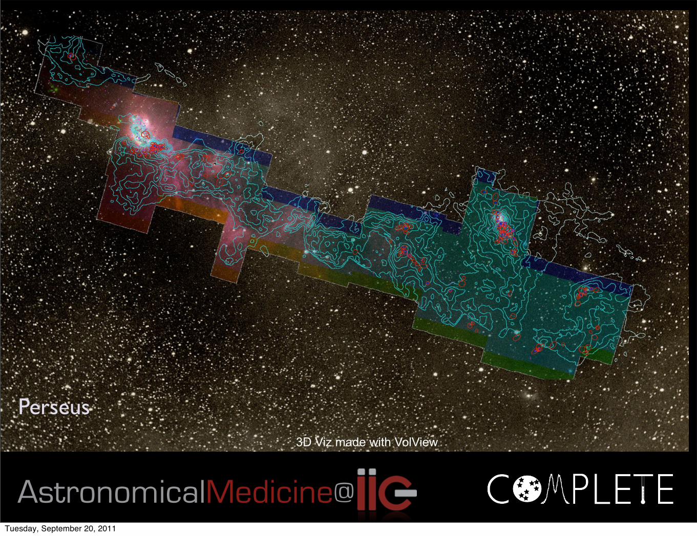
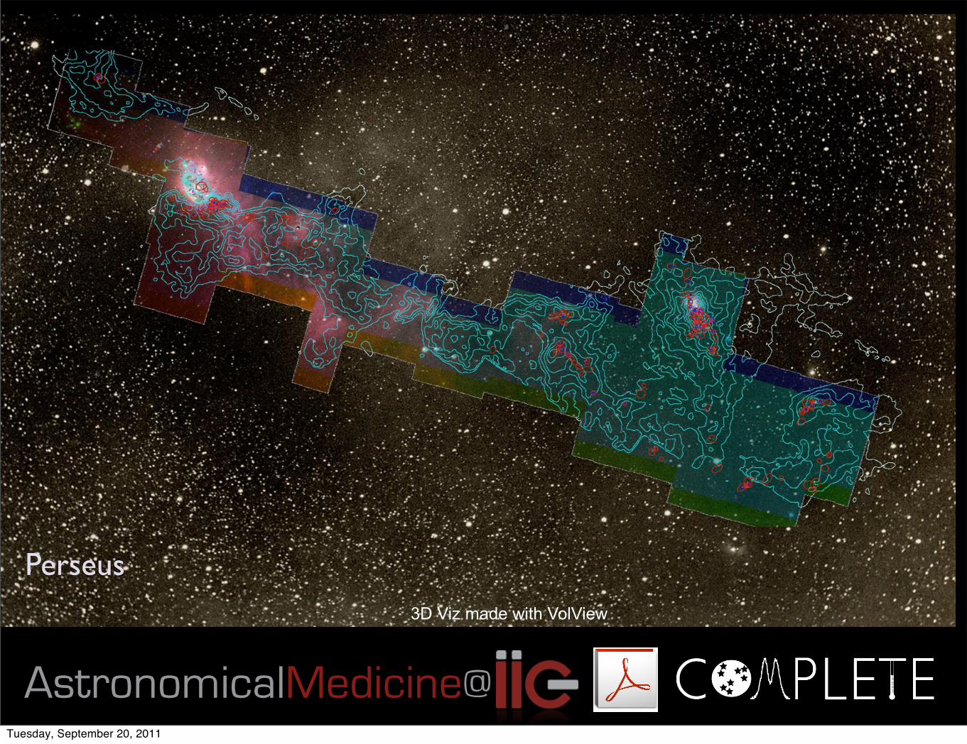
mm peak (Enoch et al. 2006)
sub-mm peak (Hatchellet al. 2005, Kirk et al. 2006)
13CO (Ridge et al. 2006)
mid-IR IRAC composite from c2d data (Foster, Laakso, Ridge, et al. in prep.)
Optical image (Barnard 1927)
Perseus
Tuesday, September 20, 2011
mm peak (Enoch et al. 2006)
sub-mm peak (Hatchellet al. 2005, Kirk et al. 2006)
13CO (Ridge et al. 2006)
mid-IR IRAC composite from c2d data (Foster, Laakso, Ridge, et al. in prep.)
Optical image (Barnard 1927)
Perseus
Tuesday, September 20, 2011

mm peak (Enoch et al. 2006)
sub-mm peak (Hatchellet al. 2005, Kirk et al. 2006)
13CO (Ridge et al. 2006)
mid-IR IRAC composite from c2d data (Foster, Laakso, Ridge, et al. in prep.)
Optical image (Barnard 1927)
Perseus
Tuesday, September 20, 2011
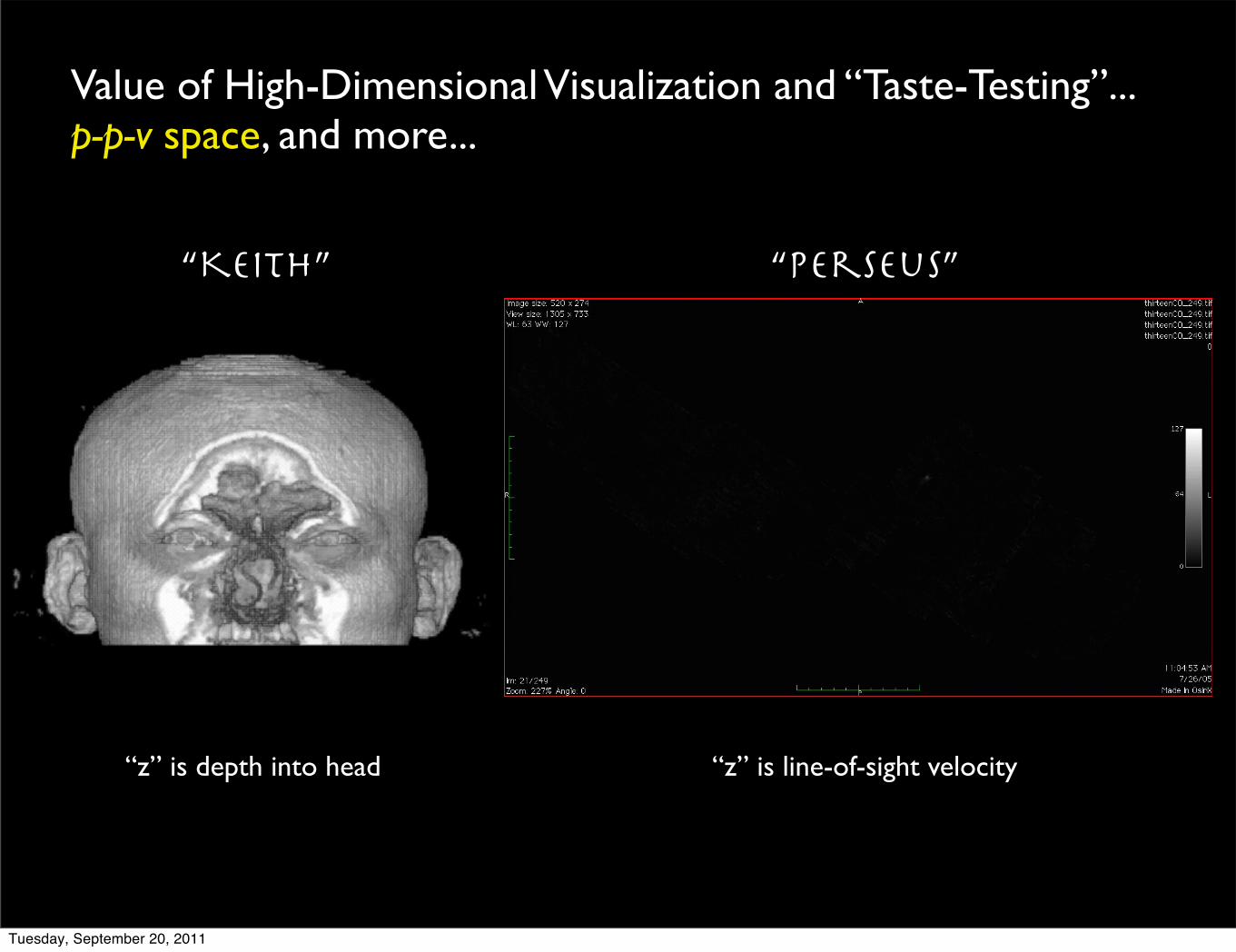
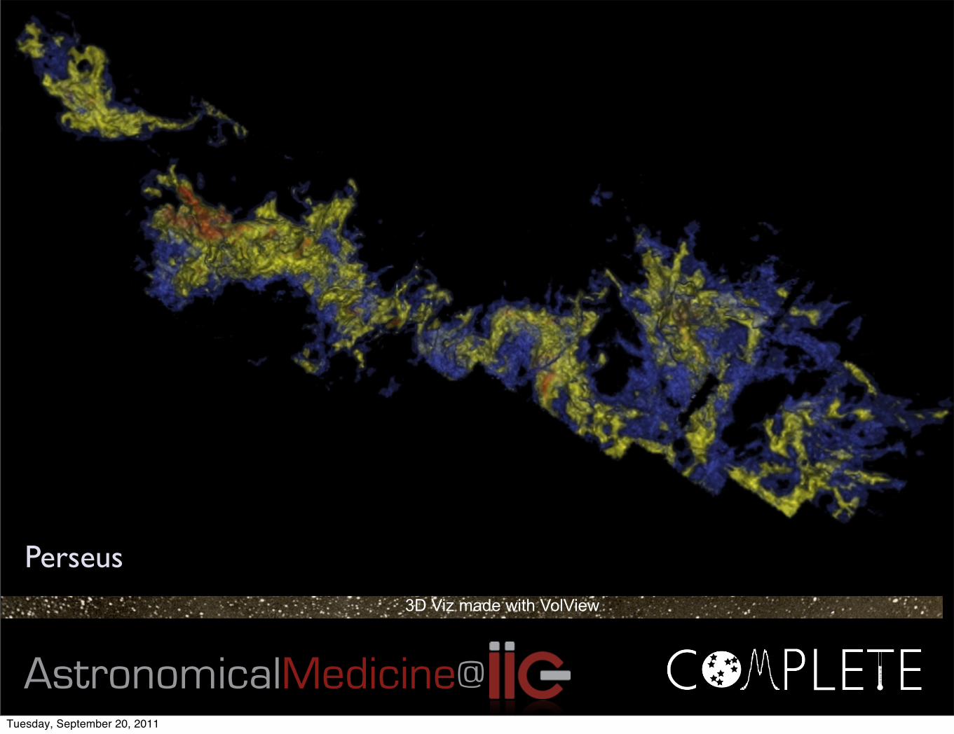
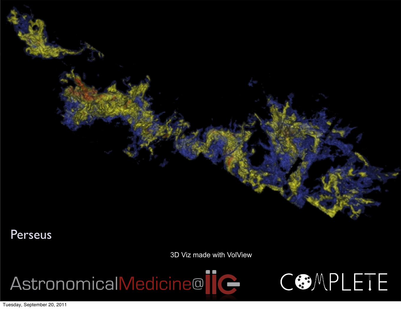
“Keith” “Perseus”
Value of High-Dimensional Visualization and “Taste-Testing”...p-p-v space, and more...
“z” is depth into head “z” is line-of-sight velocity
Tuesday, September 20, 2011
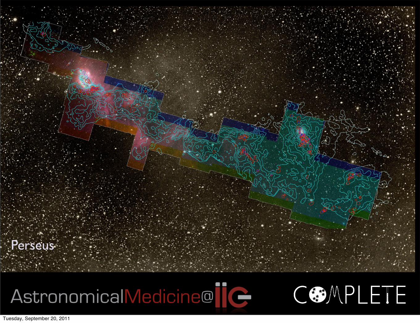
AstronomicalMedicine@
Perseus
Tuesday, September 20, 2011
AstronomicalMedicine@
3D Viz made with VolView
Perseus
Tuesday, September 20, 2011
AstronomicalMedicine@
3D Viz made with VolView
Perseus
Tuesday, September 20, 2011
AstronomicalMedicine@
3D Viz made with VolView
Perseus
Tuesday, September 20, 2011
AstronomicalMedicine@
3D Viz made with VolView
Perseus
Tuesday, September 20, 2011
Where and when does gravity matter?And, is the virial theorem over-used?
data, CLUMPFIND typically finds features on a limited range of scales,abovebut close to thephysical resolution of thedata, and its results canbe overly dependent on input parameters. By tuning CLUMPFIND’stwo free parameters, the same molecular-line data set8 can be used toshow either that the frequency distribution of clumpmass is the sameas the initial mass function of stars or that it follows the much shal-lower mass function associated with large-scale molecular clouds(Supplementary Fig. 1).
Four years before the advent of CLUMPFIND, ‘structure trees’9
were proposed as a way to characterize clouds’ hierarchical structure
using 2Dmaps of column density.With this early 2Dwork as inspira-tion, we have developed a structure-identification algorithm thatabstracts the hierarchical structure of a 3D (p–p–v) data cube intoan easily visualized representation called a ‘dendrogram’10. Althoughwell developed in other data-intensive fields11,12, it is curious that theapplication of treemethodologies so far in astrophysics has been rare,and almost exclusively within the area of galaxy evolution, where‘merger trees’ are being used with increasing frequency13.
Figure 3 and its legend explain the construction of dendrogramsschematically. The dendrogram quantifies how and where local max-ima of emission merge with each other, and its implementation isexplained in Supplementary Methods. Critically, the dendrogram isdetermined almost entirely by the data itself, and it has negligiblesensitivity to algorithm parameters. To make graphical presentationpossible on paper and 2D screens, we ‘flatten’ the dendrograms of 3Ddata (see Fig. 3 and its legend), by sorting their ‘branches’ to notcross, which eliminates dimensional information on the x axis whilepreserving all information about connectivity and hierarchy.Numbered ‘billiard ball’ labels in the figures let the reader matchfeatures between a 2D map (Fig. 1), an interactive 3D map (Fig. 2aonline) and a sorted dendrogram (Fig. 2c).
A dendrogramof a spectral-line data cube allows for the estimationof key physical properties associated with volumes bounded by iso-surfaces, such as radius (R), velocity dispersion (sv) and luminosity(L). The volumes can have any shape, and in other work14 we focus onthe significance of the especially elongated features seen in L1448(Fig. 2a). The luminosity is an approximate proxy for mass, suchthat Mlum5X13COL13CO, where X13CO5 8.03 1020 cm2K21 km21 s(ref. 15; see Supplementary Methods and Supplementary Fig. 2).The derived values for size, mass and velocity dispersion can then beused to estimate the role of self-gravity at each point in the hierarchy,via calculation of an ‘observed’ virial parameter, aobs5 5sv
2R/GMlum.In principle, extended portions of the tree (Fig. 2, yellow highlighting)where aobs, 2 (where gravitational energy is comparable to or largerthan kinetic energy) correspond to regions of p–p–v space where self-gravity is significant. As aobs only represents the ratio of kinetic energyto gravitational energy at one point in time, and does not explicitlycapture external over-pressure and/or magnetic fields16, its measuredvalue should only be used as a guide to the longevity (boundedness) ofany particular feature.
Self-gravitatingleaves
CLUMPFIND segmentation
vz
x (RA)
y (d
ec.)
vz
x (RA) y
(dec
.)
c
d
8
6
4
2
0
8
6
4
2
0
T mb
(K)
T mb
(K)
Self-gravitatingstructures
All structure
a b
Click to rotate
Figure 2 | Comparison of the ‘dendrogram’ and ‘CLUMPFIND’ feature-identification algorithms as applied to 13CO emission from the L1448region of Perseus. a, 3D visualization of the surfaces indicated by colours inthe dendrogram shown in c. Purple illustrates the smallest scale self-gravitating structures in the region corresponding to the leaves of thedendrogram; pink shows the smallest surfaces that contain distinct self-gravitating leaves within them; and green corresponds to the surface in thedata cube containing all the significant emission. Dendrogram branchescorresponding to self-gravitating objects have been highlighted in yellowover the range of Tmb (main-beam temperature) test-level values for whichthe virial parameter is less than 2. The x–y locations of the four ‘self-gravitating’ leaves labelled with billiard balls are the same as those shown inFig. 1. The 3D visualizations showposition–position–velocity (p–p–v) space.RA, right ascension; dec., declination. For comparison with the ability ofdendrograms (c) to track hierarchical structure, d shows a pseudo-dendrogram of the CLUMPFIND segmentation (b), with the same fourlabels used in Fig. 1 and in a. As ‘clumps’ are not allowed to belong to largerstructures, each pseudo-branch in d is simply a series of lines connecting themaximum emission value in each clump to the threshold value. A very largenumber of clumps appears in b because of the sensitivity of CLUMPFIND tonoise and small-scale structure in the data. In the online PDF version, the 3Dcubes (a and b) can be rotated to any orientation, and surfaces can be turnedon and off (interaction requires Adobe Acrobat version 7.0.8 or higher). Inthe printed version, the front face of each 3D cube (the ‘home’ view in theinteractive online version) corresponds exactly to the patch of sky shown inFig. 1, and velocity with respect to the Local Standard of Rest increases fromfront (20.5 km s21) to back (8 km s21).
Inte
nsity
leve
l
Local max
Local max
Local max
Merge
Merge
Leaf
Leaf
Leaf
Bra
nch
Trun
k
Test level
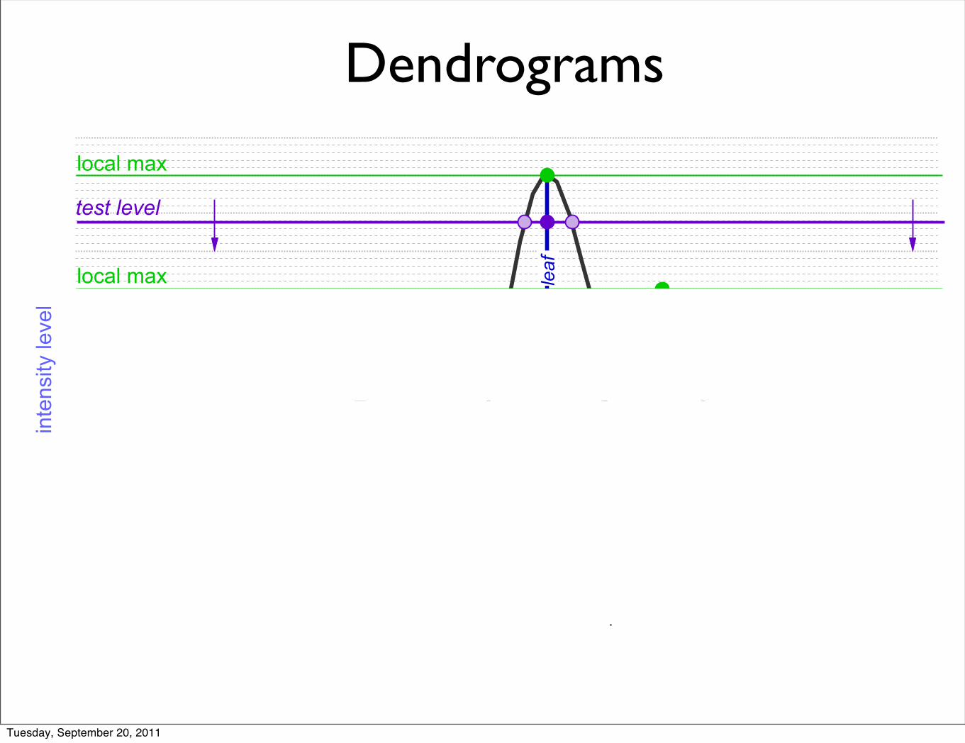
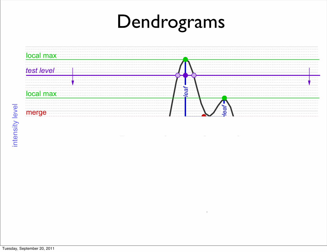
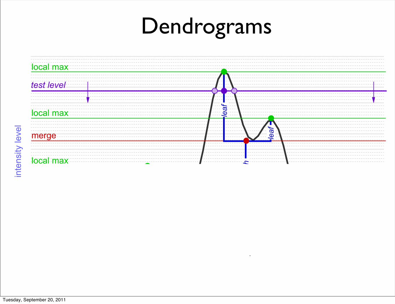
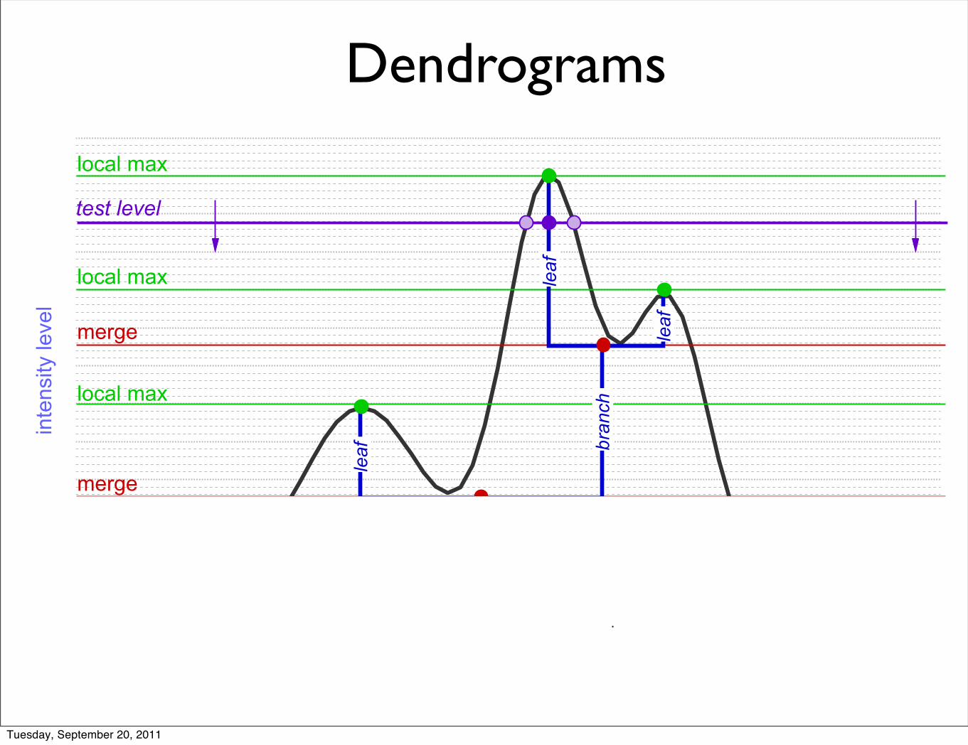
Figure 3 | Schematic illustration of the dendrogram process. Shown is theconstruction of a dendrogram from a hypothetical one-dimensionalemission profile (black). The dendrogram (blue) can be constructed by‘dropping’ a test constant emission level (purple) from above in tiny steps(exaggerated in size here, light lines) until all the local maxima and mergersare found, and connected as shown. The intersection of a test level with theemission is a set of points (for example the light purple dots) in onedimension, a planar curve in two dimensions, and an isosurface in threedimensions. The dendrogram of 3D data shown in Fig. 2c is the directanalogue of the tree shown here, only constructed from ‘isosurface’ ratherthan ‘point’ intersections. It has been sorted and flattened for representationon a flat page, as fully representing dendrograms for 3D data cubes wouldrequire four dimensions.
LETTERS NATURE |Vol 457 | 1 January 2009
64 Macmillan Publishers Limited. All rights reserved©2009
Goodman et al. 2009 Shetty et al. 2010
IS the virial theorem over-used?
Tuesday, September 20, 2011
Where and when does gravity matter?And, is the virial theorem over-used?
data, CLUMPFIND typically finds features on a limited range of scales,abovebut close to thephysical resolution of thedata, and its results canbe overly dependent on input parameters. By tuning CLUMPFIND’stwo free parameters, the same molecular-line data set8 can be used toshow either that the frequency distribution of clumpmass is the sameas the initial mass function of stars or that it follows the much shal-lower mass function associated with large-scale molecular clouds(Supplementary Fig. 1).
Four years before the advent of CLUMPFIND, ‘structure trees’9
were proposed as a way to characterize clouds’ hierarchical structure
using 2Dmaps of column density.With this early 2Dwork as inspira-tion, we have developed a structure-identification algorithm thatabstracts the hierarchical structure of a 3D (p–p–v) data cube intoan easily visualized representation called a ‘dendrogram’10. Althoughwell developed in other data-intensive fields11,12, it is curious that theapplication of treemethodologies so far in astrophysics has been rare,and almost exclusively within the area of galaxy evolution, where‘merger trees’ are being used with increasing frequency13.
Figure 3 and its legend explain the construction of dendrogramsschematically. The dendrogram quantifies how and where local max-ima of emission merge with each other, and its implementation isexplained in Supplementary Methods. Critically, the dendrogram isdetermined almost entirely by the data itself, and it has negligiblesensitivity to algorithm parameters. To make graphical presentationpossible on paper and 2D screens, we ‘flatten’ the dendrograms of 3Ddata (see Fig. 3 and its legend), by sorting their ‘branches’ to notcross, which eliminates dimensional information on the x axis whilepreserving all information about connectivity and hierarchy.Numbered ‘billiard ball’ labels in the figures let the reader matchfeatures between a 2D map (Fig. 1), an interactive 3D map (Fig. 2aonline) and a sorted dendrogram (Fig. 2c).
A dendrogramof a spectral-line data cube allows for the estimationof key physical properties associated with volumes bounded by iso-surfaces, such as radius (R), velocity dispersion (sv) and luminosity(L). The volumes can have any shape, and in other work14 we focus onthe significance of the especially elongated features seen in L1448(Fig. 2a). The luminosity is an approximate proxy for mass, suchthat Mlum5X13COL13CO, where X13CO5 8.03 1020 cm2K21 km21 s(ref. 15; see Supplementary Methods and Supplementary Fig. 2).The derived values for size, mass and velocity dispersion can then beused to estimate the role of self-gravity at each point in the hierarchy,via calculation of an ‘observed’ virial parameter, aobs5 5sv
2R/GMlum.In principle, extended portions of the tree (Fig. 2, yellow highlighting)where aobs, 2 (where gravitational energy is comparable to or largerthan kinetic energy) correspond to regions of p–p–v space where self-gravity is significant. As aobs only represents the ratio of kinetic energyto gravitational energy at one point in time, and does not explicitlycapture external over-pressure and/or magnetic fields16, its measuredvalue should only be used as a guide to the longevity (boundedness) ofany particular feature.
Self-gravitatingleaves
CLUMPFIND segmentation
vz
x (RA)
y (d
ec.)
vz
x (RA) y
(dec
.)
c
d
8
6
4
2
0
8
6
4
2
0
T mb
(K)
T mb
(K)
Self-gravitatingstructures
All structure
a b
Click to rotate
Figure 2 | Comparison of the ‘dendrogram’ and ‘CLUMPFIND’ feature-identification algorithms as applied to 13CO emission from the L1448region of Perseus. a, 3D visualization of the surfaces indicated by colours inthe dendrogram shown in c. Purple illustrates the smallest scale self-gravitating structures in the region corresponding to the leaves of thedendrogram; pink shows the smallest surfaces that contain distinct self-gravitating leaves within them; and green corresponds to the surface in thedata cube containing all the significant emission. Dendrogram branchescorresponding to self-gravitating objects have been highlighted in yellowover the range of Tmb (main-beam temperature) test-level values for whichthe virial parameter is less than 2. The x–y locations of the four ‘self-gravitating’ leaves labelled with billiard balls are the same as those shown inFig. 1. The 3D visualizations showposition–position–velocity (p–p–v) space.RA, right ascension; dec., declination. For comparison with the ability ofdendrograms (c) to track hierarchical structure, d shows a pseudo-dendrogram of the CLUMPFIND segmentation (b), with the same fourlabels used in Fig. 1 and in a. As ‘clumps’ are not allowed to belong to largerstructures, each pseudo-branch in d is simply a series of lines connecting themaximum emission value in each clump to the threshold value. A very largenumber of clumps appears in b because of the sensitivity of CLUMPFIND tonoise and small-scale structure in the data. In the online PDF version, the 3Dcubes (a and b) can be rotated to any orientation, and surfaces can be turnedon and off (interaction requires Adobe Acrobat version 7.0.8 or higher). Inthe printed version, the front face of each 3D cube (the ‘home’ view in theinteractive online version) corresponds exactly to the patch of sky shown inFig. 1, and velocity with respect to the Local Standard of Rest increases fromfront (20.5 km s21) to back (8 km s21).
Inte
nsity
leve
l
Local max
Local max
Local max
Merge
Merge
Leaf
Leaf
Leaf
Bra
nch
Trun
k
Test level
Figure 3 | Schematic illustration of the dendrogram process. Shown is theconstruction of a dendrogram from a hypothetical one-dimensionalemission profile (black). The dendrogram (blue) can be constructed by‘dropping’ a test constant emission level (purple) from above in tiny steps(exaggerated in size here, light lines) until all the local maxima and mergersare found, and connected as shown. The intersection of a test level with theemission is a set of points (for example the light purple dots) in onedimension, a planar curve in two dimensions, and an isosurface in threedimensions. The dendrogram of 3D data shown in Fig. 2c is the directanalogue of the tree shown here, only constructed from ‘isosurface’ ratherthan ‘point’ intersections. It has been sorted and flattened for representationon a flat page, as fully representing dendrograms for 3D data cubes wouldrequire four dimensions.
LETTERS NATURE |Vol 457 | 1 January 2009
64 Macmillan Publishers Limited. All rights reserved©2009
Goodman et al. 2009 Shetty et al. 2010
IS the virial theorem over-used?
Tuesday, September 20, 2011
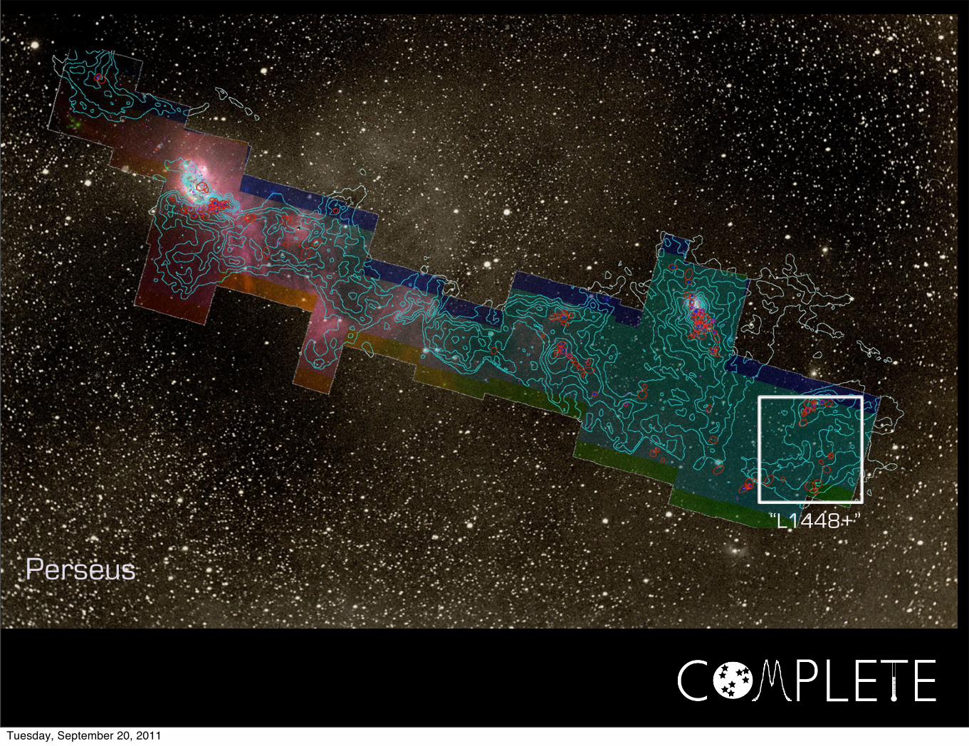
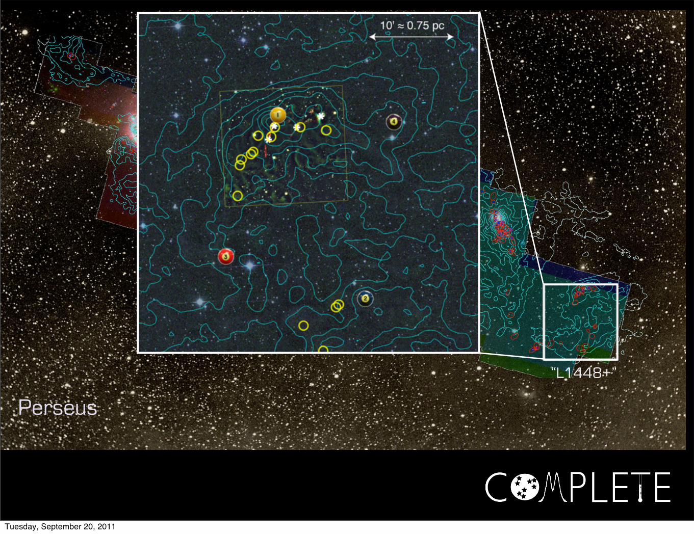
Perseus
“L1448+”
Tuesday, September 20, 2011
Perseus
“L1448+”
Tuesday, September 20, 2011
Perseus
“L1448+”
Tuesday, September 20, 2011
Dendrograms1.20
1.10
1.00
0.90
0.80
0.70
0.60
0.50
0.40
0.30
0.20
0.10
0.00
80 70 60 50 40 30 20
inte
nsity
leve
l
local max
local max
local max
merge
merge
Hierarchical “Segmentation”Rosolowsky, Pineda, Kauffmann & Goodman 2008
Tuesday, September 20, 2011
Dendrograms1.20
1.10
1.00
0.90
0.80
0.70
0.60
0.50
0.40
0.30
0.20
0.10
0.00
80 70 60 50 40 30 20
inte
nsity
leve
l
local max
local max
local max
merge
merge
Tuesday, September 20, 2011
Dendrograms1.20
1.10
1.00
0.90
0.80
0.70
0.60
0.50
0.40
0.30
0.20
0.10
0.00
80 70 60 50 40 30 20
inte
nsity
leve
l
local max
local max
local max
merge
merge
Tuesday, September 20, 2011
Dendrograms1.20
1.10
1.00
0.90
0.80
0.70
0.60
0.50
0.40
0.30
0.20
0.10
0.00
80 70 60 50 40 30 20
inte
nsity
leve
l
local max
local max
local max
merge
merge
Tuesday, September 20, 2011
Dendrograms1.20
1.10
1.00
0.90
0.80
0.70
0.60
0.50
0.40
0.30
0.20
0.10
0.00
80 70 60 50 40 30 20
inte
nsity
leve
l
local max
local max
local max
merge
merge
Tuesday, September 20, 2011
Dendrograms1.20
1.10
1.00
0.90
0.80
0.70
0.60
0.50
0.40
0.30
0.20
0.10
0.00
80 70 60 50 40 30 20
inte
nsity
leve
l
local max
local max
local max
merge
merge
Tuesday, September 20, 2011
Dendrograms1.20
1.10
1.00
0.90
0.80
0.70
0.60
0.50
0.40
0.30
0.20
0.10
0.00
80 70 60 50 40 30 20
inte
nsity
leve
l
local max
local max
local max
merge
merge
Tuesday, September 20, 2011
Dendrograms1.20
1.10
1.00
0.90
0.80
0.70
0.60
0.50
0.40
0.30
0.20
0.10
0.00
80 70 60 50 40 30 20
inte
nsity
leve
l
local max
local max
local max
merge
merge
1-D: points; 2-D closed curves (contours); 3-D surfaces enclosing volumessee 2D demo at http://am.iic.harvard.edu/index.cgi/DendroStar/applet
Tuesday, September 20, 2011
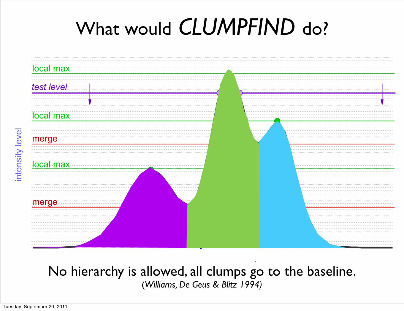
What would CLUMPFIND do?1.20
1.10
1.00
0.90
0.80
0.70
0.60
0.50
0.40
0.30
0.20
0.10
0.00
80 70 60 50 40 30 20
inte
nsity
leve
l
local max
local max
local max
merge
merge
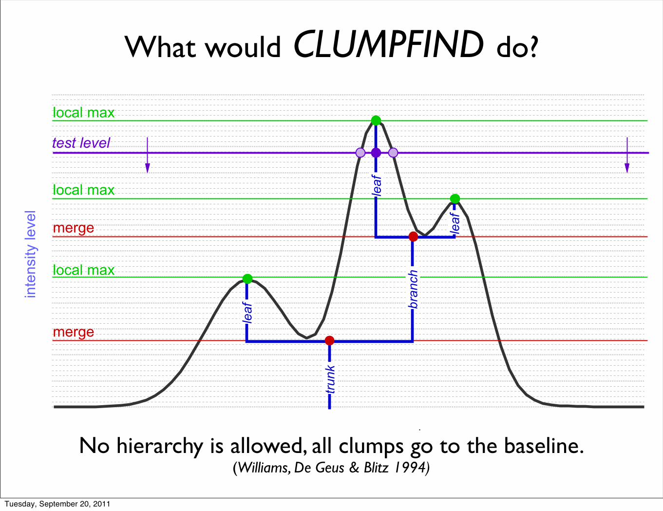
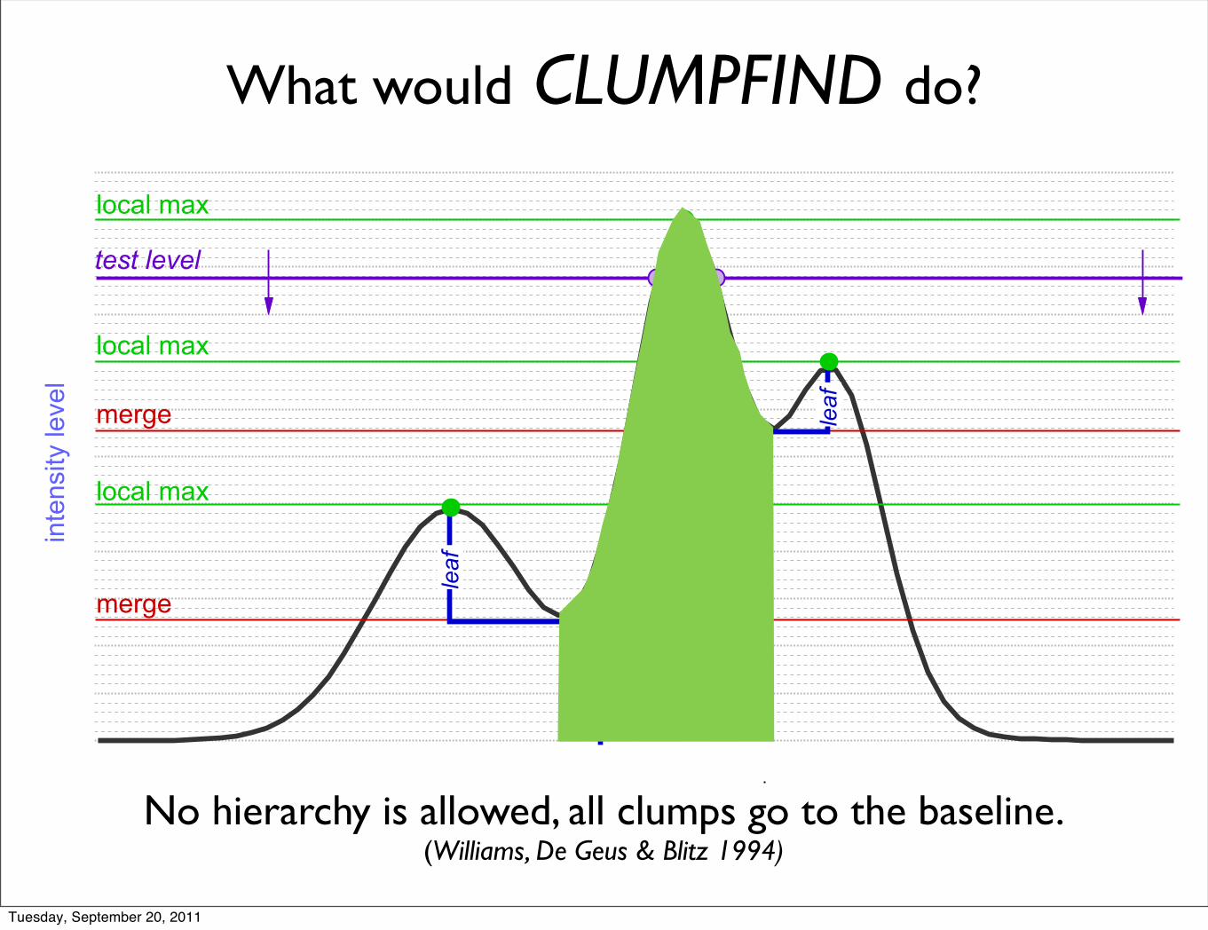
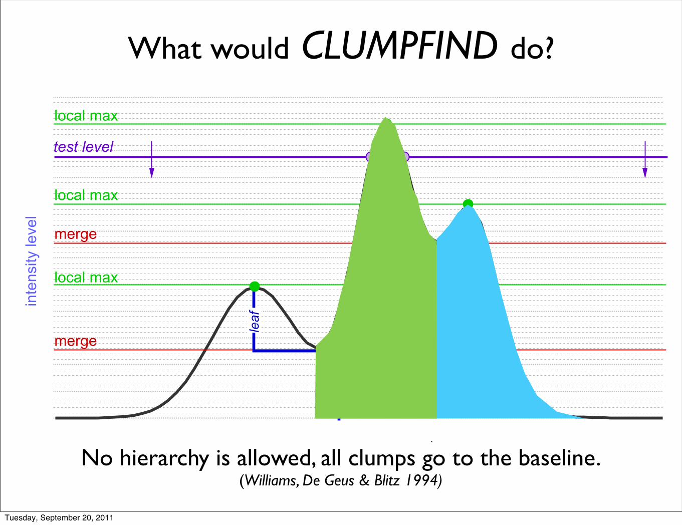
No hierarchy is allowed, all clumps go to the baseline.(Williams, De Geus & Blitz 1994)
Tuesday, September 20, 2011
What would CLUMPFIND do?1.20
1.10
1.00
0.90
0.80
0.70
0.60
0.50
0.40
0.30
0.20
0.10
0.00
80 70 60 50 40 30 20
inte
nsity
leve
l
local max
local max
local max
merge
merge
No hierarchy is allowed, all clumps go to the baseline.(Williams, De Geus & Blitz 1994)
Tuesday, September 20, 2011
What would CLUMPFIND do?1.20
1.10
1.00
0.90
0.80
0.70
0.60
0.50
0.40
0.30
0.20
0.10
0.00
80 70 60 50 40 30 20
inte
nsity
leve
l
local max
local max
local max
merge
merge
No hierarchy is allowed, all clumps go to the baseline.(Williams, De Geus & Blitz 1994)
Tuesday, September 20, 2011
What would CLUMPFIND do?1.20
1.10
1.00
0.90
0.80
0.70
0.60
0.50
0.40
0.30
0.20
0.10
0.00
80 70 60 50 40 30 20
inte
nsity
leve
l
local max
local max
local max
merge
merge
No hierarchy is allowed, all clumps go to the baseline.(Williams, De Geus & Blitz 1994)
Tuesday, September 20, 2011

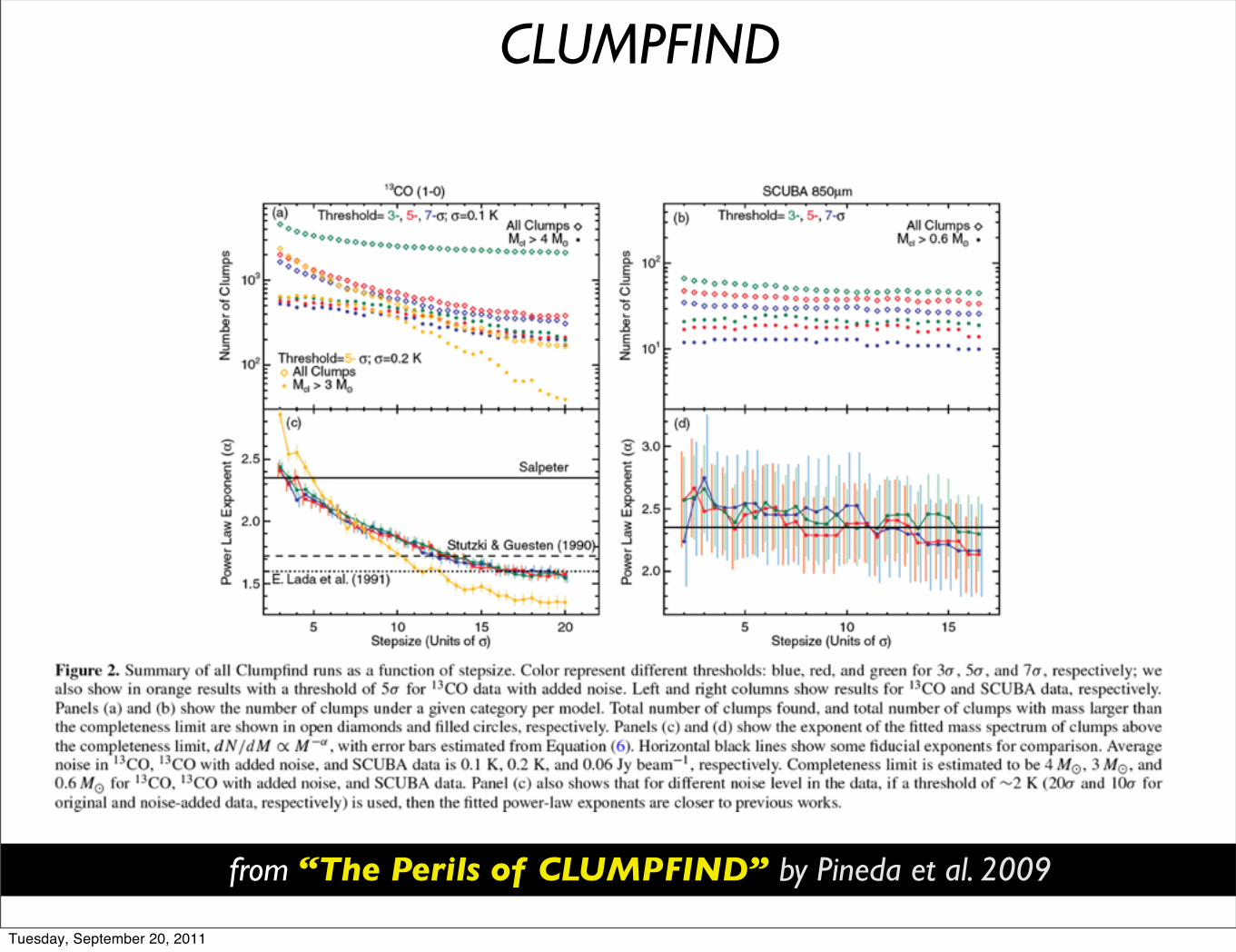
from “The Perils of CLUMPFIND” by Pineda et al. 2009
CLUMPFIND
Tuesday, September 20, 2011
from “The Perils of CLUMPFIND” by Pineda et al. 2009
CLUMPFIND
Tuesday, September 20, 2011
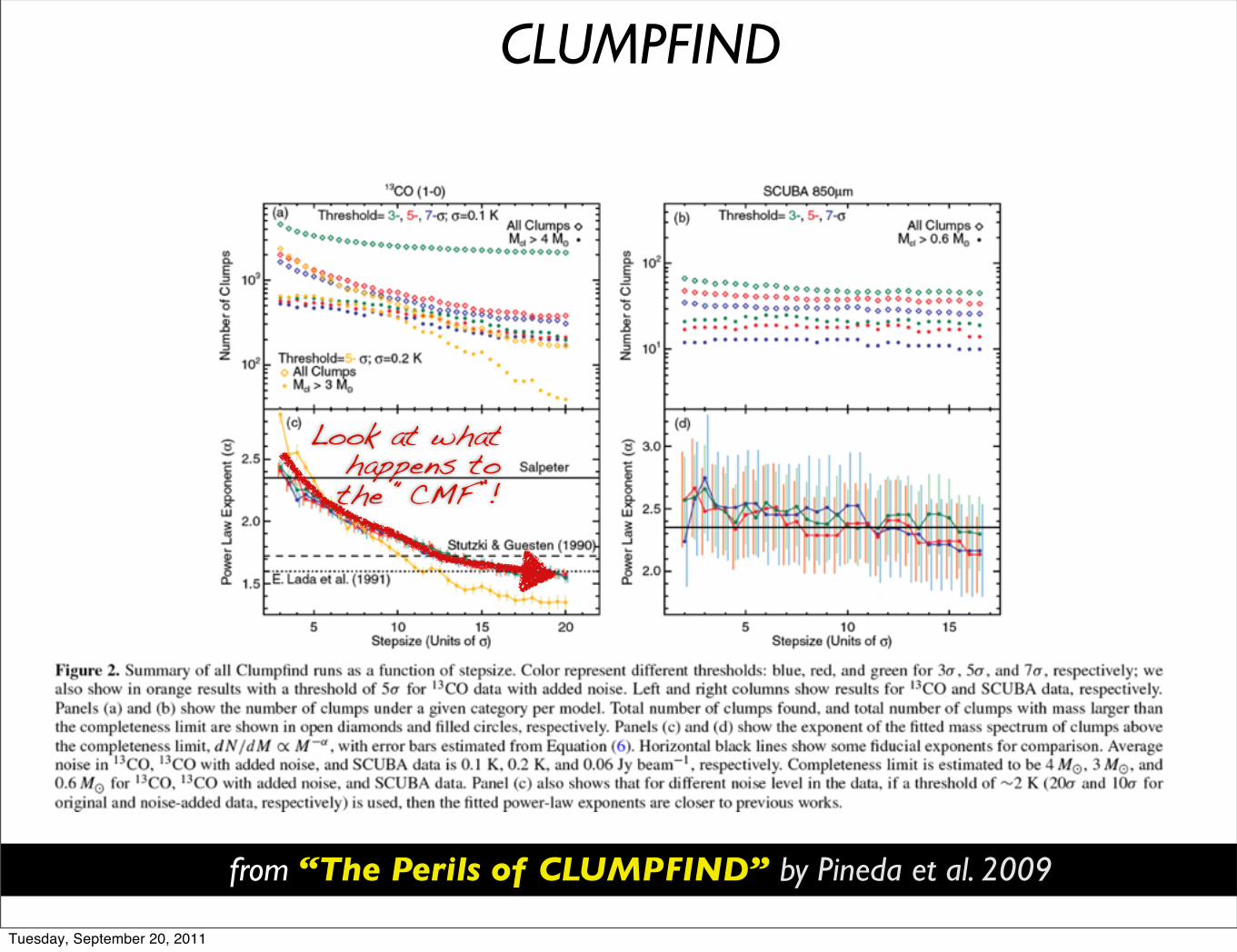
from “The Perils of CLUMPFIND” by Pineda et al. 2009
Look at what happens to the “CMF”!
CLUMPFIND
Tuesday, September 20, 2011
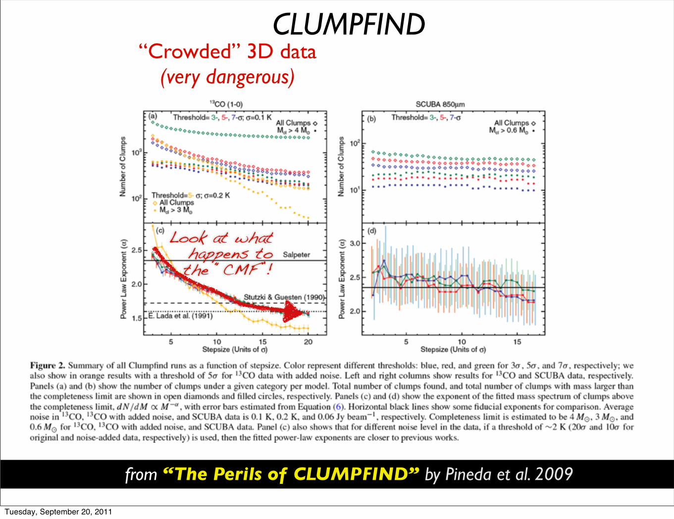
from “The Perils of CLUMPFIND” by Pineda et al. 2009
“Crowded” 3D data(very dangerous)
Look at what happens to the “CMF”!
CLUMPFIND
Tuesday, September 20, 2011
from “The Perils of CLUMPFIND” by Pineda et al. 2009
“Crowded” 3D data(very dangerous)
“Sparse” 2D data(OK)
Look at what happens to the “CMF”!
CLUMPFIND
Tuesday, September 20, 2011
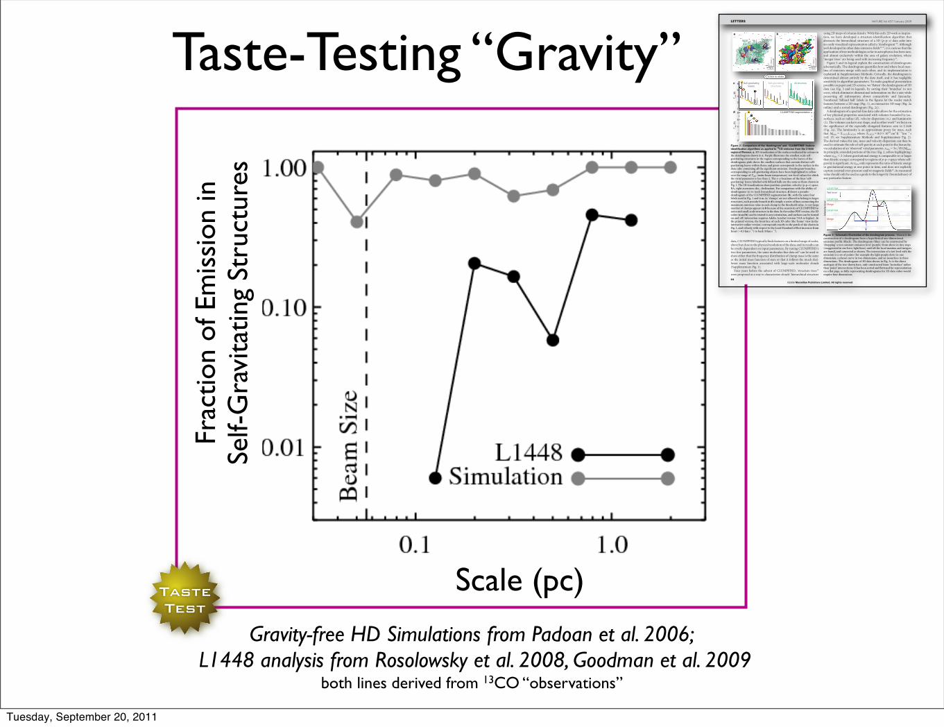
Taste-Testing “Gravity”
Frac
tion
of E
mis
sion
in
Self-
Gra
vita
ting
Stru
ctur
es
Scale (pc)Taste Test
Gravity-free HD Simulations from Padoan et al. 2006; L1448 analysis from Rosolowsky et al. 2008, Goodman et al. 2009
both lines derived from 13CO “observations”
data, CLUMPFIND typically finds features on a limited range of scales,abovebut close to thephysical resolution of thedata, and its results canbe overly dependent on input parameters. By tuning CLUMPFIND’stwo free parameters, the same molecular-line data set8 can be used toshow either that the frequency distribution of clumpmass is the sameas the initial mass function of stars or that it follows the much shal-lower mass function associated with large-scale molecular clouds(Supplementary Fig. 1).
Four years before the advent of CLUMPFIND, ‘structure trees’9
were proposed as a way to characterize clouds’ hierarchical structure
using 2Dmaps of column density.With this early 2Dwork as inspira-tion, we have developed a structure-identification algorithm thatabstracts the hierarchical structure of a 3D (p–p–v) data cube intoan easily visualized representation called a ‘dendrogram’10. Althoughwell developed in other data-intensive fields11,12, it is curious that theapplication of treemethodologies so far in astrophysics has been rare,and almost exclusively within the area of galaxy evolution, where‘merger trees’ are being used with increasing frequency13.
Figure 3 and its legend explain the construction of dendrogramsschematically. The dendrogram quantifies how and where local max-ima of emission merge with each other, and its implementation isexplained in Supplementary Methods. Critically, the dendrogram isdetermined almost entirely by the data itself, and it has negligiblesensitivity to algorithm parameters. To make graphical presentationpossible on paper and 2D screens, we ‘flatten’ the dendrograms of 3Ddata (see Fig. 3 and its legend), by sorting their ‘branches’ to notcross, which eliminates dimensional information on the x axis whilepreserving all information about connectivity and hierarchy.Numbered ‘billiard ball’ labels in the figures let the reader matchfeatures between a 2D map (Fig. 1), an interactive 3D map (Fig. 2aonline) and a sorted dendrogram (Fig. 2c).
A dendrogramof a spectral-line data cube allows for the estimationof key physical properties associated with volumes bounded by iso-surfaces, such as radius (R), velocity dispersion (sv) and luminosity(L). The volumes can have any shape, and in other work14 we focus onthe significance of the especially elongated features seen in L1448(Fig. 2a). The luminosity is an approximate proxy for mass, suchthat Mlum5X13COL13CO, where X13CO5 8.03 1020 cm2K21 km21 s(ref. 15; see Supplementary Methods and Supplementary Fig. 2).The derived values for size, mass and velocity dispersion can then beused to estimate the role of self-gravity at each point in the hierarchy,via calculation of an ‘observed’ virial parameter, aobs5 5sv
2R/GMlum.In principle, extended portions of the tree (Fig. 2, yellow highlighting)where aobs, 2 (where gravitational energy is comparable to or largerthan kinetic energy) correspond to regions of p–p–v space where self-gravity is significant. As aobs only represents the ratio of kinetic energyto gravitational energy at one point in time, and does not explicitlycapture external over-pressure and/or magnetic fields16, its measuredvalue should only be used as a guide to the longevity (boundedness) ofany particular feature.
Self-gravitatingleaves
CLUMPFIND segmentation
vz
x (RA)
y (d
ec.)
vz
x (RA)
y (d
ec.)
c
d
8
6
4
2
0
8
6
4
2
0
T mb
(K)
T mb
(K)
Self-gravitatingstructures
All structure
a b
Click to rotate
Figure 2 | Comparison of the ‘dendrogram’ and ‘CLUMPFIND’ feature-identification algorithms as applied to 13CO emission from the L1448region of Perseus. a, 3D visualization of the surfaces indicated by colours inthe dendrogram shown in c. Purple illustrates the smallest scale self-gravitating structures in the region corresponding to the leaves of thedendrogram; pink shows the smallest surfaces that contain distinct self-gravitating leaves within them; and green corresponds to the surface in thedata cube containing all the significant emission. Dendrogram branchescorresponding to self-gravitating objects have been highlighted in yellowover the range of Tmb (main-beam temperature) test-level values for whichthe virial parameter is less than 2. The x–y locations of the four ‘self-gravitating’ leaves labelled with billiard balls are the same as those shown inFig. 1. The 3D visualizations showposition–position–velocity (p–p–v) space.RA, right ascension; dec., declination. For comparison with the ability ofdendrograms (c) to track hierarchical structure, d shows a pseudo-dendrogram of the CLUMPFIND segmentation (b), with the same fourlabels used in Fig. 1 and in a. As ‘clumps’ are not allowed to belong to largerstructures, each pseudo-branch in d is simply a series of lines connecting themaximum emission value in each clump to the threshold value. A very largenumber of clumps appears in b because of the sensitivity of CLUMPFIND tonoise and small-scale structure in the data. In the online PDF version, the 3Dcubes (a and b) can be rotated to any orientation, and surfaces can be turnedon and off (interaction requires Adobe Acrobat version 7.0.8 or higher). Inthe printed version, the front face of each 3D cube (the ‘home’ view in theinteractive online version) corresponds exactly to the patch of sky shown inFig. 1, and velocity with respect to the Local Standard of Rest increases fromfront (20.5 km s21) to back (8 km s21).
Inte
nsity
leve
l
Local max
Local max
Local max
Merge
Merge
Leaf
Leaf
Leaf
Bra
nch
Trun
k
Test level
Figure 3 | Schematic illustration of the dendrogram process. Shown is theconstruction of a dendrogram from a hypothetical one-dimensionalemission profile (black). The dendrogram (blue) can be constructed by‘dropping’ a test constant emission level (purple) from above in tiny steps(exaggerated in size here, light lines) until all the local maxima and mergersare found, and connected as shown. The intersection of a test level with theemission is a set of points (for example the light purple dots) in onedimension, a planar curve in two dimensions, and an isosurface in threedimensions. The dendrogram of 3D data shown in Fig. 2c is the directanalogue of the tree shown here, only constructed from ‘isosurface’ ratherthan ‘point’ intersections. It has been sorted and flattened for representationon a flat page, as fully representing dendrograms for 3D data cubes wouldrequire four dimensions.
LETTERS NATURE |Vol 457 | 1 January 2009
64 Macmillan Publishers Limited. All rights reserved©2009
Tuesday, September 20, 2011
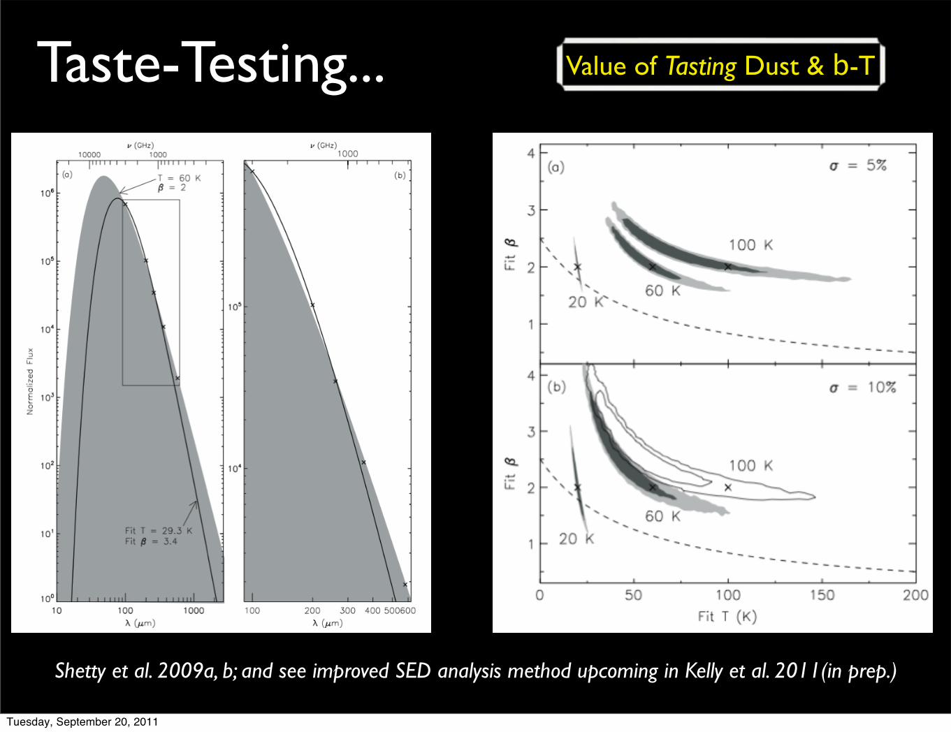
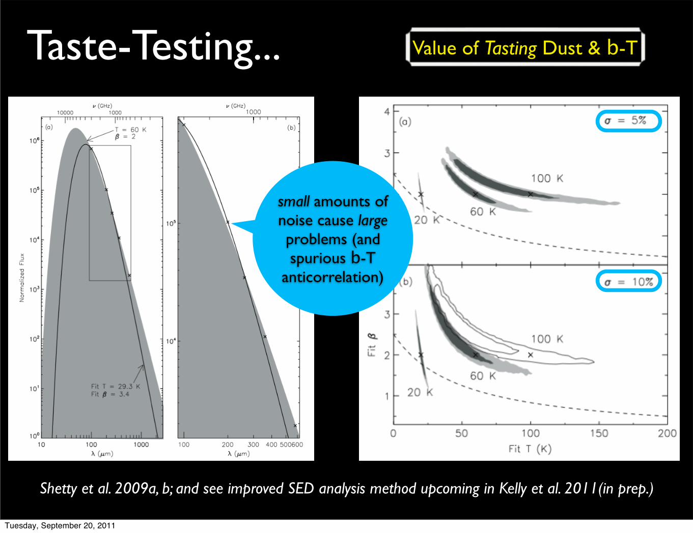
Taste-Testing... Value of Tasting Dust & b-T
Shetty et al. 2009a, b; and see improved SED analysis method upcoming in Kelly et al. 2011(in prep.)
Tuesday, September 20, 2011
Taste-Testing... Value of Tasting Dust & b-T
Shetty et al. 2009a, b; and see improved SED analysis method upcoming in Kelly et al. 2011(in prep.)
small amounts of noise cause large problems (and spurious b-T
anticorrelation)
Tuesday, September 20, 2011
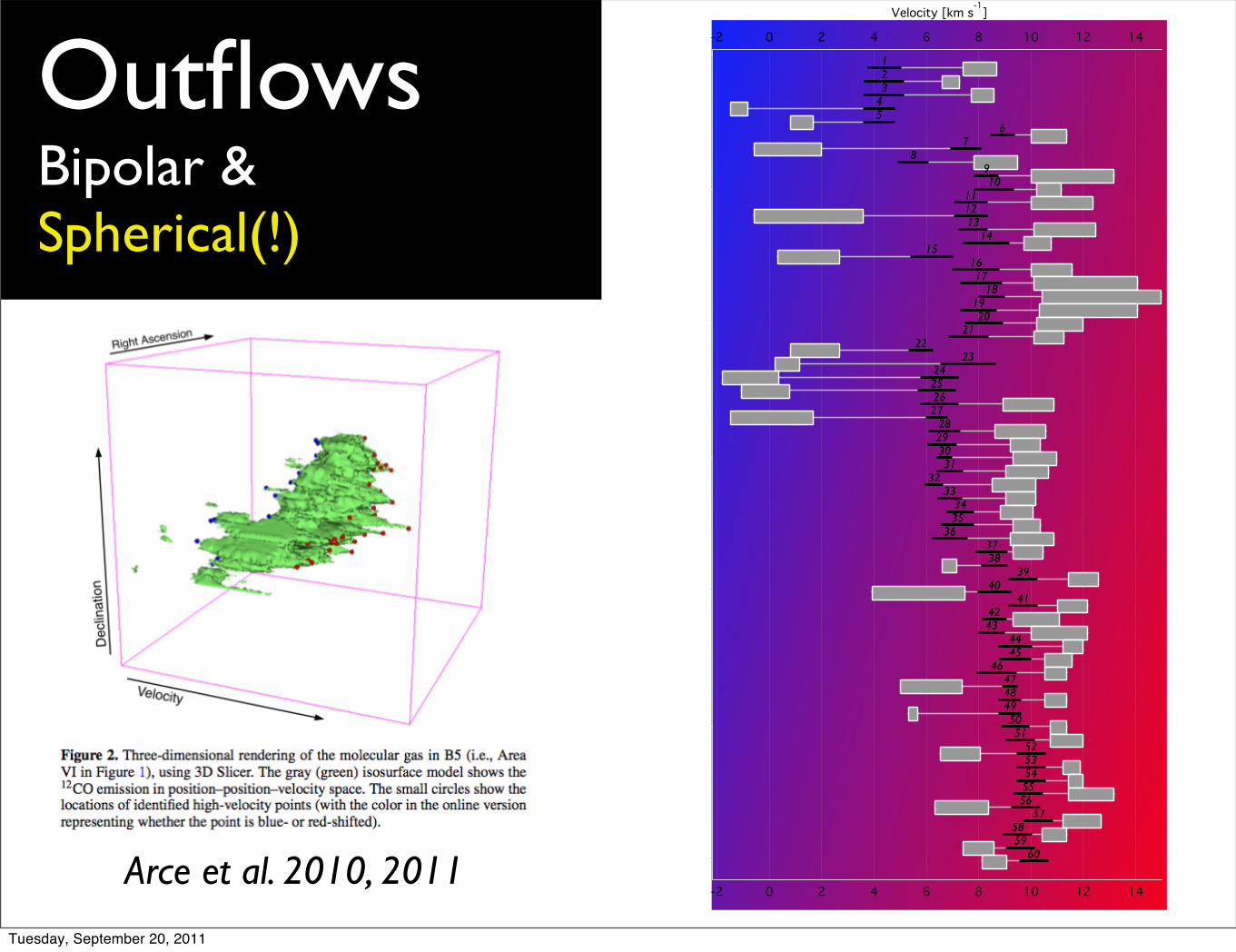
Arce et al. 2010, 2011
OutflowsBipolar & Spherical(!)
Tuesday, September 20, 2011
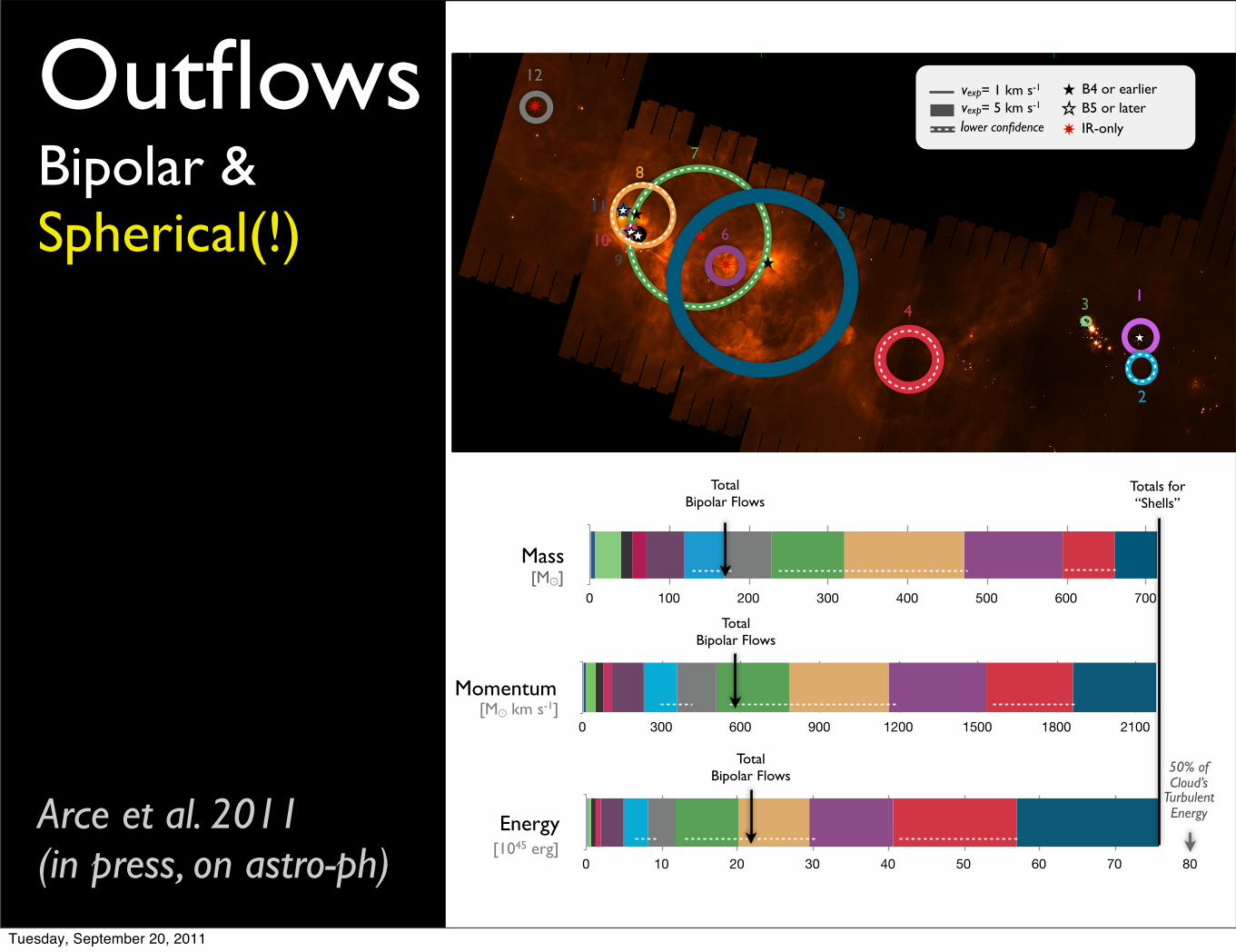
Momentum
0 300 600 900 1200 1500 1800 2100 2400 2700 3000
910
11
7
6
1
2
34
8
5
12
vexp= 5 km s-1vexp= 1 km s-1 B4 or earlier
B5 or laterIR-only
Total Bipolar Flows
Totals for“Shells”
Mass
0 100 200 300 400 500 600 700 800
Energy
0 10 20 30 40 50 60 70 80
50% of Cloud’s
Turbulent Energy
5 pc
lower confidence
Total Bipolar Flows
Total Bipolar Flows
[M]
[M km s-1]
[1045 erg]
Arce et al. 2011(in press, on astro-ph)
OutflowsBipolar & Spherical(!)
Tuesday, September 20, 2011
Momentum
0 300 600 900 1200 1500 1800 2100 2400 2700 3000
910
11
7
6
1
2
34
8
5
12
vexp= 5 km s-1vexp= 1 km s-1 B4 or earlier
B5 or laterIR-only
Total Bipolar Flows
Totals for“Shells”
Mass
0 100 200 300 400 500 600 700 800
Energy
0 10 20 30 40 50 60 70 80
50% of Cloud’s
Turbulent Energy
5 pc
lower confidence
Total Bipolar Flows
Total Bipolar Flows
[M]
[M km s-1]
[1045 erg]
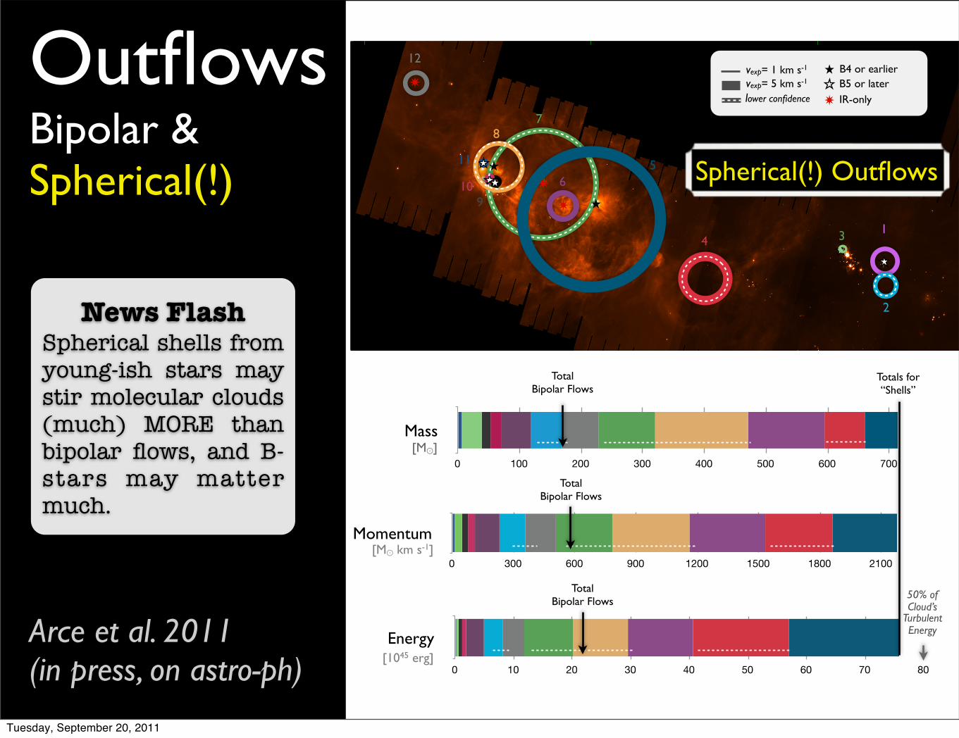
Arce et al. 2011(in press, on astro-ph)
OutflowsBipolar & Spherical(!)
News FlashSpherical shells from young-ish stars may stir molecular clouds (much) MORE than bipolar flows, and B-stars may matter much.
Spherical(!) Outflows
Tuesday, September 20, 2011
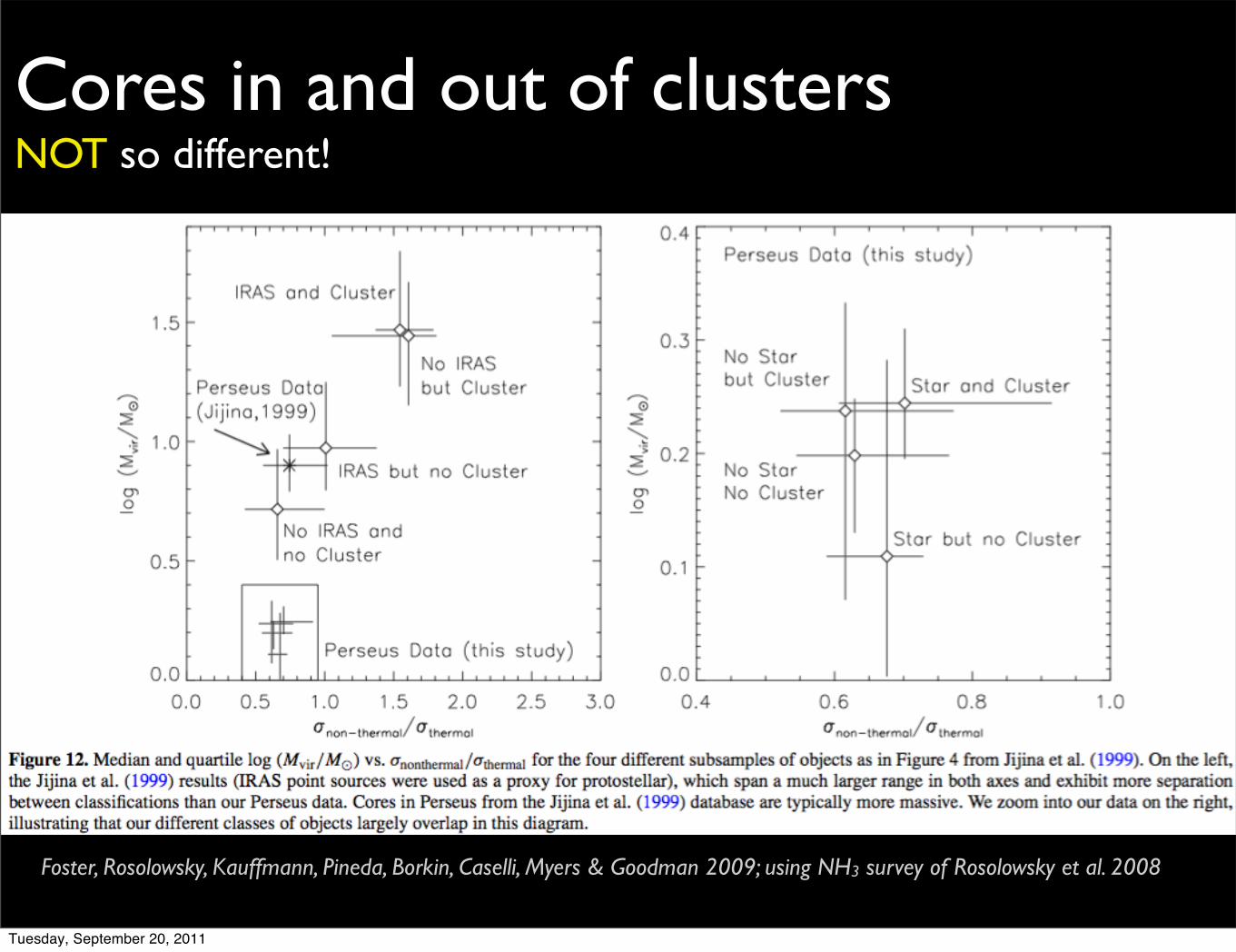
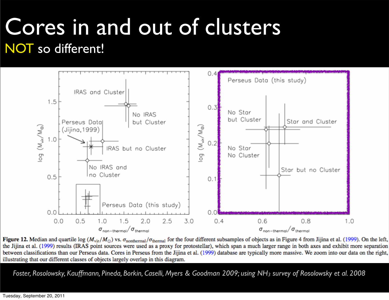
Cores in and out of clustersNOT so different!
Foster, Rosolowsky, Kauffmann, Pineda, Borkin, Caselli, Myers & Goodman 2009; using NH3 survey of Rosolowsky et al. 2008
Tuesday, September 20, 2011
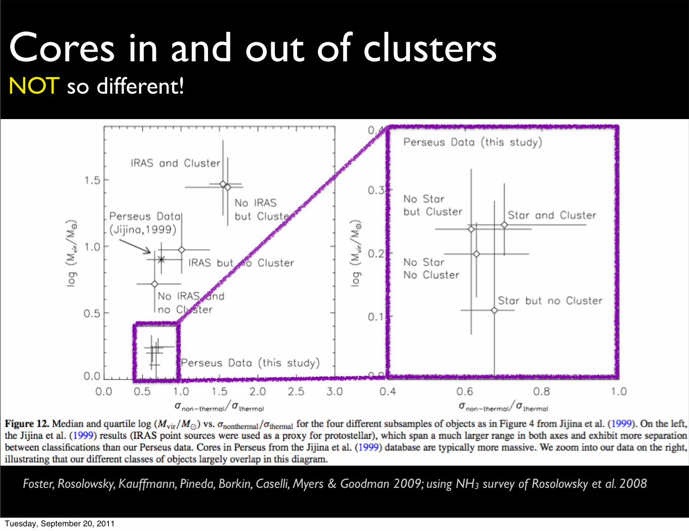
Cores in and out of clustersNOT so different!
Foster, Rosolowsky, Kauffmann, Pineda, Borkin, Caselli, Myers & Goodman 2009; using NH3 survey of Rosolowsky et al. 2008
Tuesday, September 20, 2011
Cores in and out of clustersNOT so different!
Foster, Rosolowsky, Kauffmann, Pineda, Borkin, Caselli, Myers & Goodman 2009; using NH3 survey of Rosolowsky et al. 2008
Tuesday, September 20, 2011
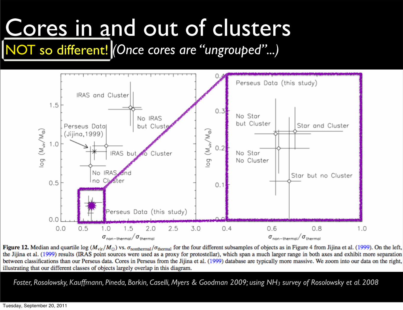
Cores in and out of clustersNOT so different!
Foster, Rosolowsky, Kauffmann, Pineda, Borkin, Caselli, Myers & Goodman 2009; using NH3 survey of Rosolowsky et al. 2008
(Once cores are “ungrouped”...)NOT so different!
Tuesday, September 20, 2011
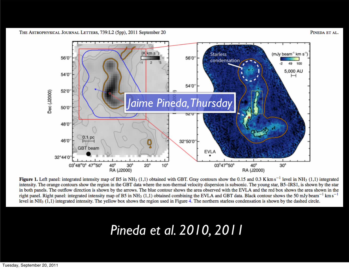
The transition to coherence has been observed directly, thanks to GBT, EVLA, and Jaime Pineda--who will tell you all about this on Wednesday!
Coherent Cores are Real, and they Fragment (into filaments)!?
Pineda et al. 2010, 2011
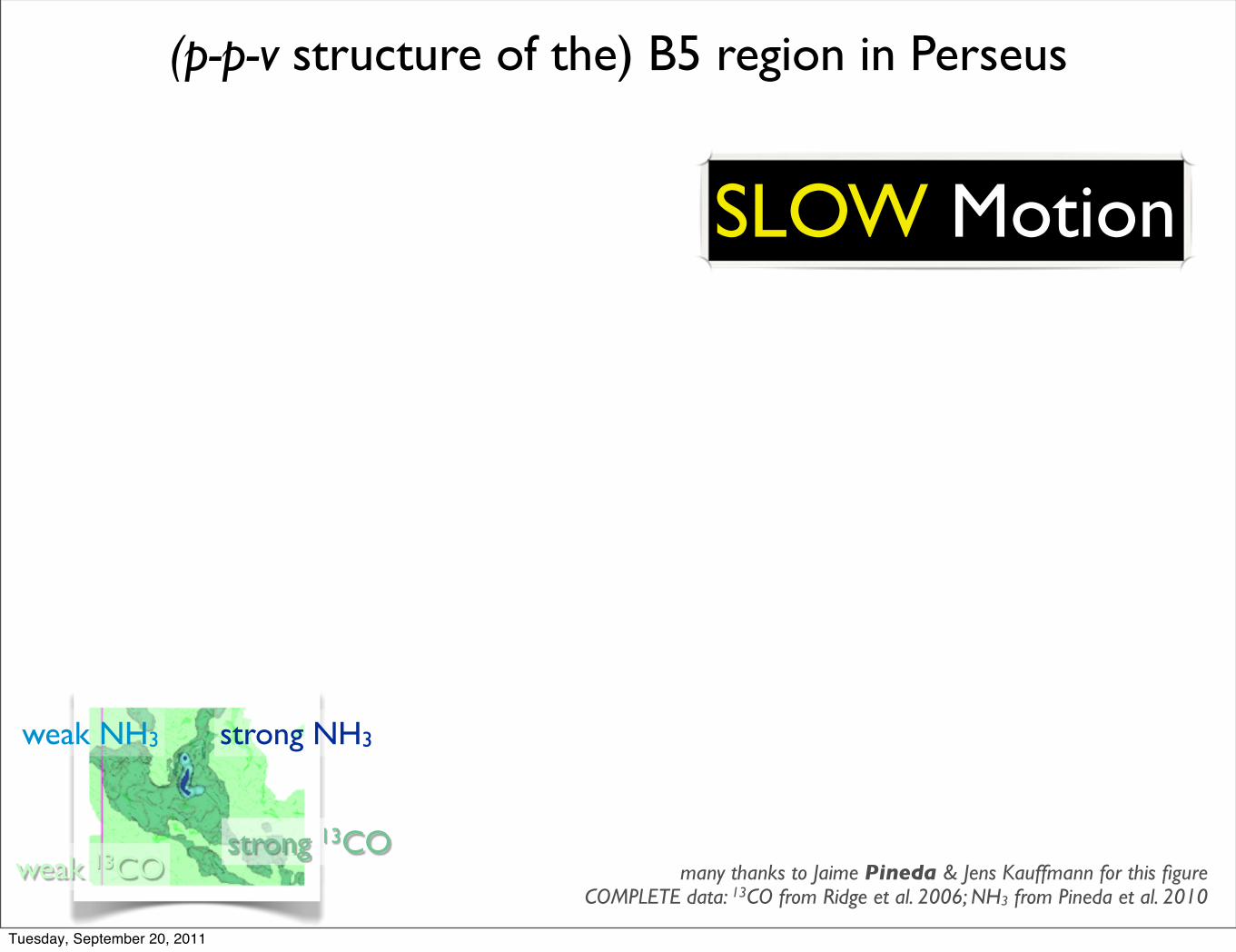
(p-p-v structure of the) B5 region in Perseus
Tuesday, September 20, 2011
The transition to coherence has been observed directly, thanks to GBT, EVLA, and Jaime Pineda--who will tell you all about this on Wednesday!
Coherent Cores are Real, and they Fragment (into filaments)!?
Pineda et al. 2010, 2011
(p-p-v structure of the) B5 region in Perseus
Jaime Pineda, Thursday
Tuesday, September 20, 2011
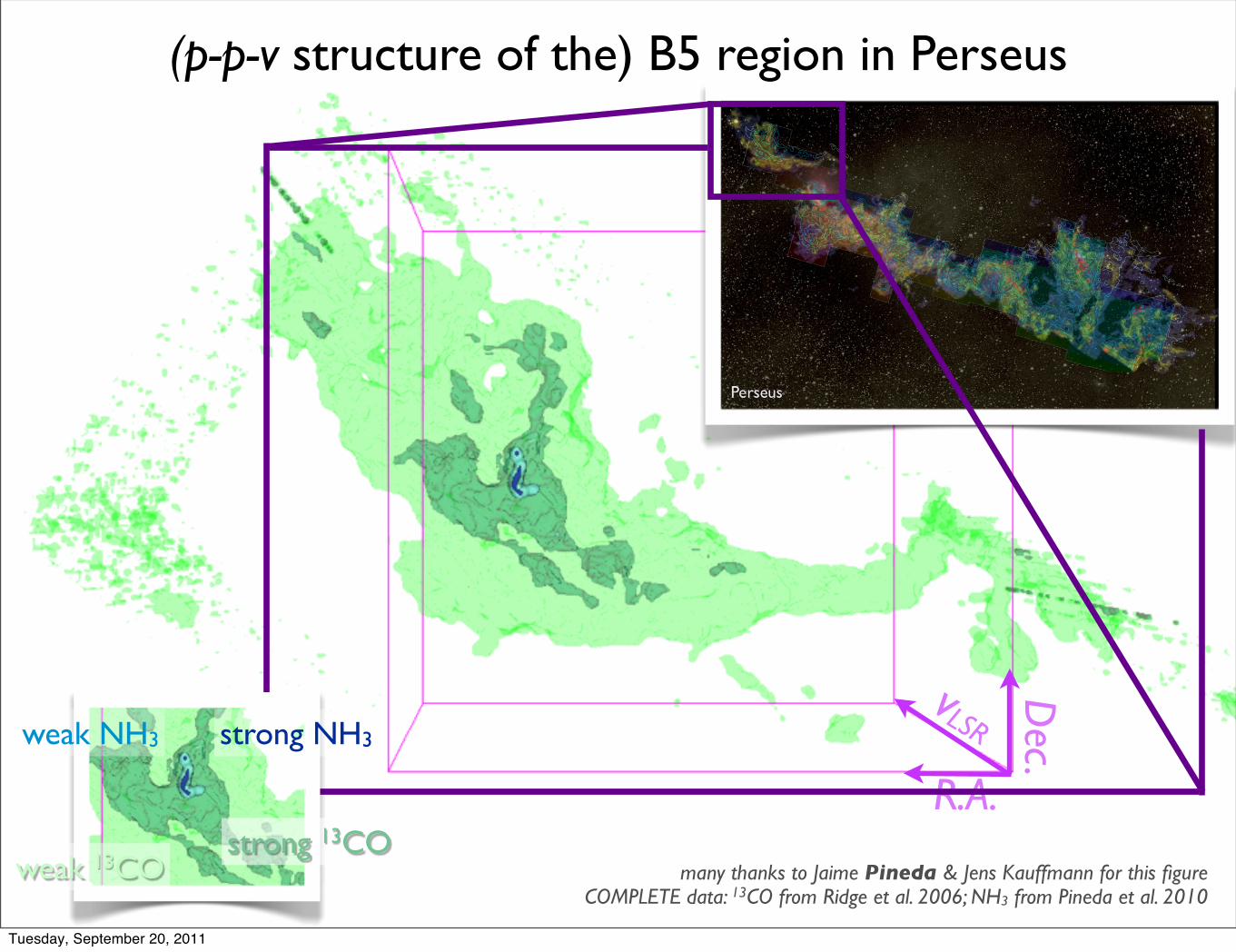
R.A.
Dec.
vLSR
many thanks to Jaime Pineda & Jens Kauffmann for this figureCOMPLETE data: 13CO from Ridge et al. 2006; NH3 from Pineda et al. 2010
weak 13COstrong 13CO
weak NH3 strong NH3
(p-p-v structure of the) B5 region in Perseus
Tuesday, September 20, 2011
R.A.
Dec.
vLSR
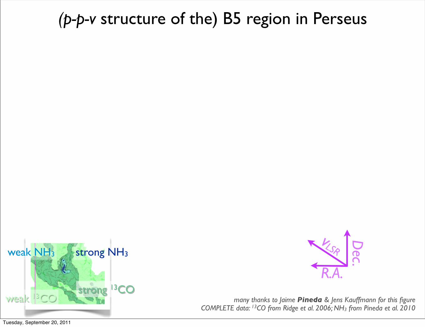
(p-p-v structure of the) B5 region in Perseus
many thanks to Jaime Pineda & Jens Kauffmann for this figureCOMPLETE data: 13CO from Ridge et al. 2006; NH3 from Pineda et al. 2010
weak 13COstrong 13CO
weak NH3 strong NH3
Tuesday, September 20, 2011
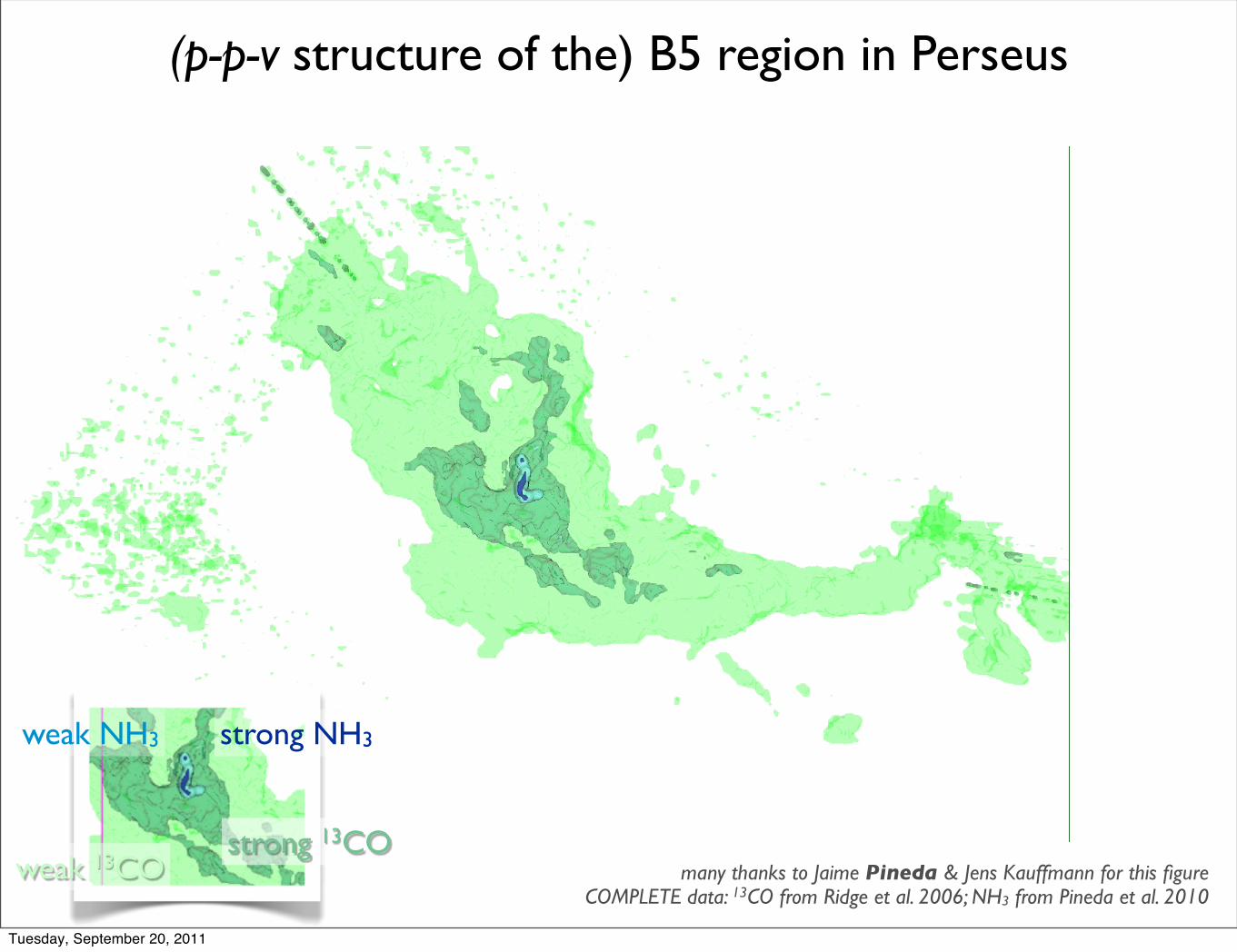
(p-p-v structure of the) B5 region in Perseus
many thanks to Jaime Pineda & Jens Kauffmann for this figureCOMPLETE data: 13CO from Ridge et al. 2006; NH3 from Pineda et al. 2010
weak 13COstrong 13CO
weak NH3 strong NH3
Tuesday, September 20, 2011
(p-p-v structure of the) B5 region in Perseus
many thanks to Jaime Pineda & Jens Kauffmann for this figureCOMPLETE data: 13CO from Ridge et al. 2006; NH3 from Pineda et al. 2010
weak 13COstrong 13CO
weak NH3 strong NH3
SLOW Motion
Tuesday, September 20, 2011

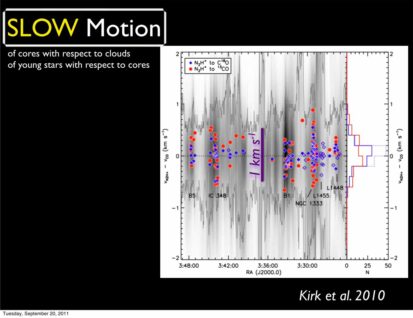
Kirk et al. 2010
of cores with respect to cloudsof young stars with respect to cores
SLOW Motion
Tuesday, September 20, 2011
Kirk et al. 2010
of cores with respect to cloudsof young stars with respect to cores
1 km
s-1
SLOW Motion
Tuesday, September 20, 2011
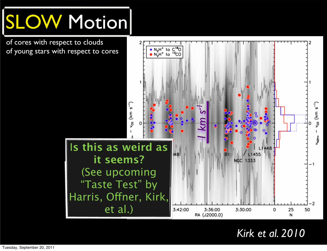
Kirk et al. 2010
Is this as weird as it seems?
(See upcoming “Taste Test” by
Harris, Offner, Kirk, et al.)
of cores with respect to cloudsof young stars with respect to cores
1 km
s-1
SLOW Motion
Tuesday, September 20, 2011

Kirk et al. 2010
of cores with respect to cloudsof young stars with respect to cores
1 km
s-1
SLOW Motion
Tuesday, September 20, 2011
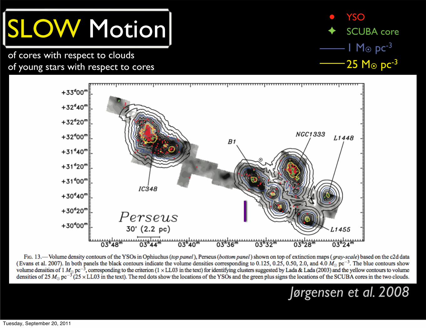
Jørgensen et al. 2008,
1 M pc-3
25 M pc-3
SCUBA coreYSO
of cores with respect to cloudsof young stars with respect to cores
SLOW Motion
Tuesday, September 20, 2011
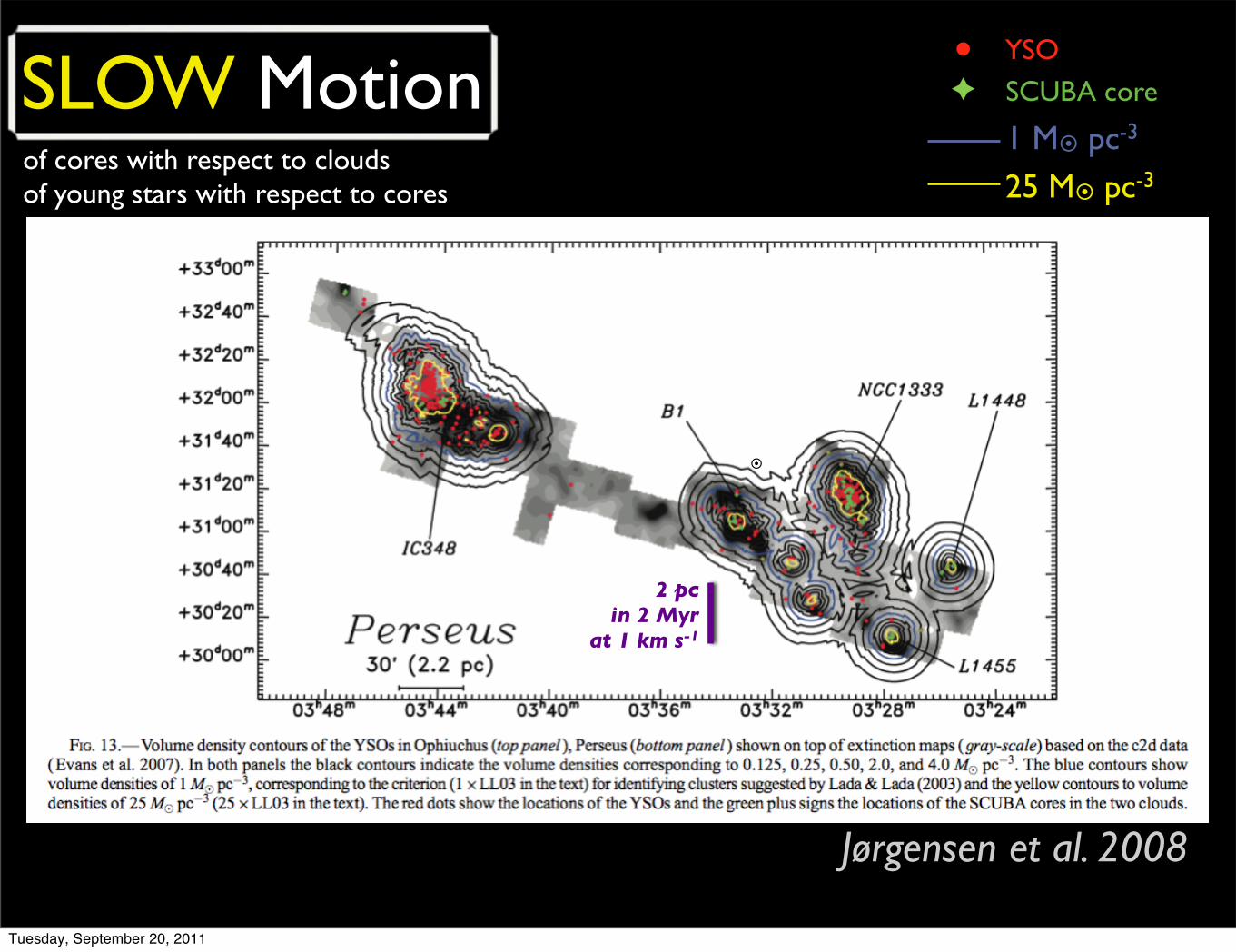
Jørgensen et al. 2008,
1 M pc-3
25 M pc-3
SCUBA coreYSO
2 pc in 2 Myr
at 1 km s-1
of cores with respect to cloudsof young stars with respect to cores
SLOW Motion
Tuesday, September 20, 2011
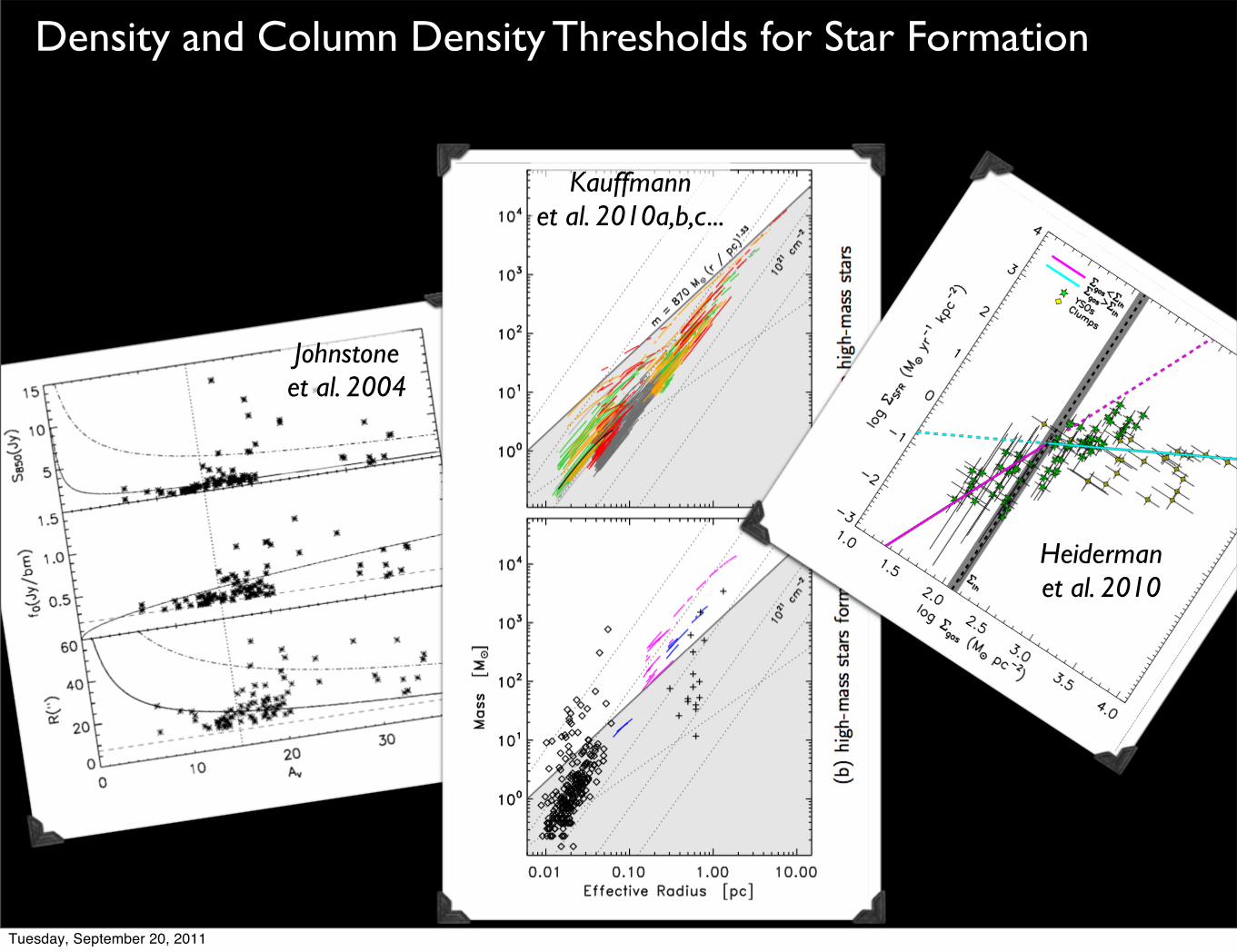
Density and Column Density Thresholds for Star Formation
Kauffmann et al. 2010a,b,c...
Heiderman et al. 2010
Johnstone et al. 2004
Tuesday, September 20, 2011
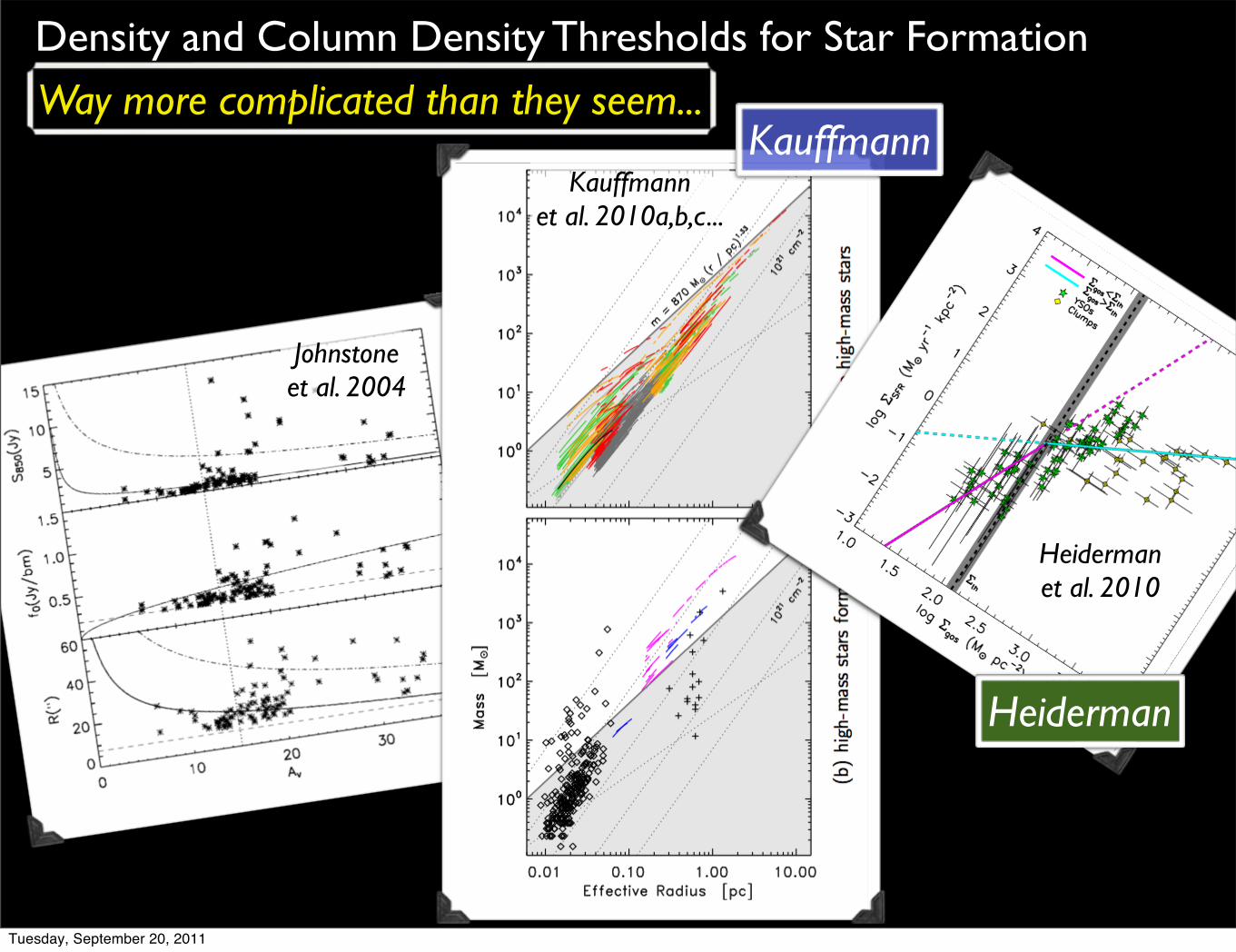
Density and Column Density Thresholds for Star Formation
Kauffmann et al. 2010a,b,c...
Heiderman et al. 2010
Johnstone et al. 2004
KauffmannWay more complicated than they seem...
Heiderman
Tuesday, September 20, 2011
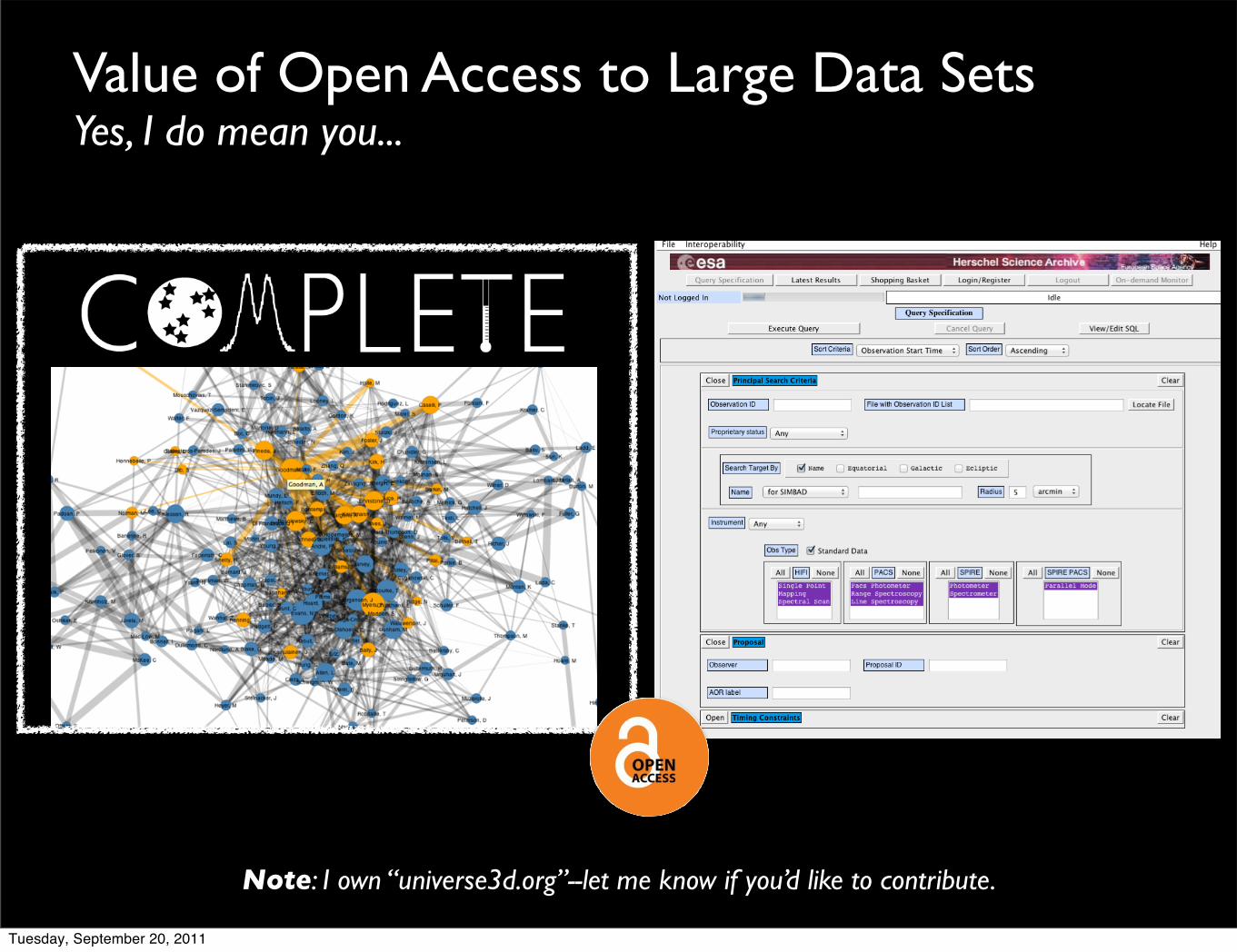
~900 citations, 10% to data paper...
H-index of 17, normalized H-index=
(17 papers)/(5 years since data paper)
=3.5!
Value of Open Access to Large Data SetsYes, I do mean you...
Note: I own “universe3d.org”--let me know if you’d like to contribute.
Tuesday, September 20, 2011
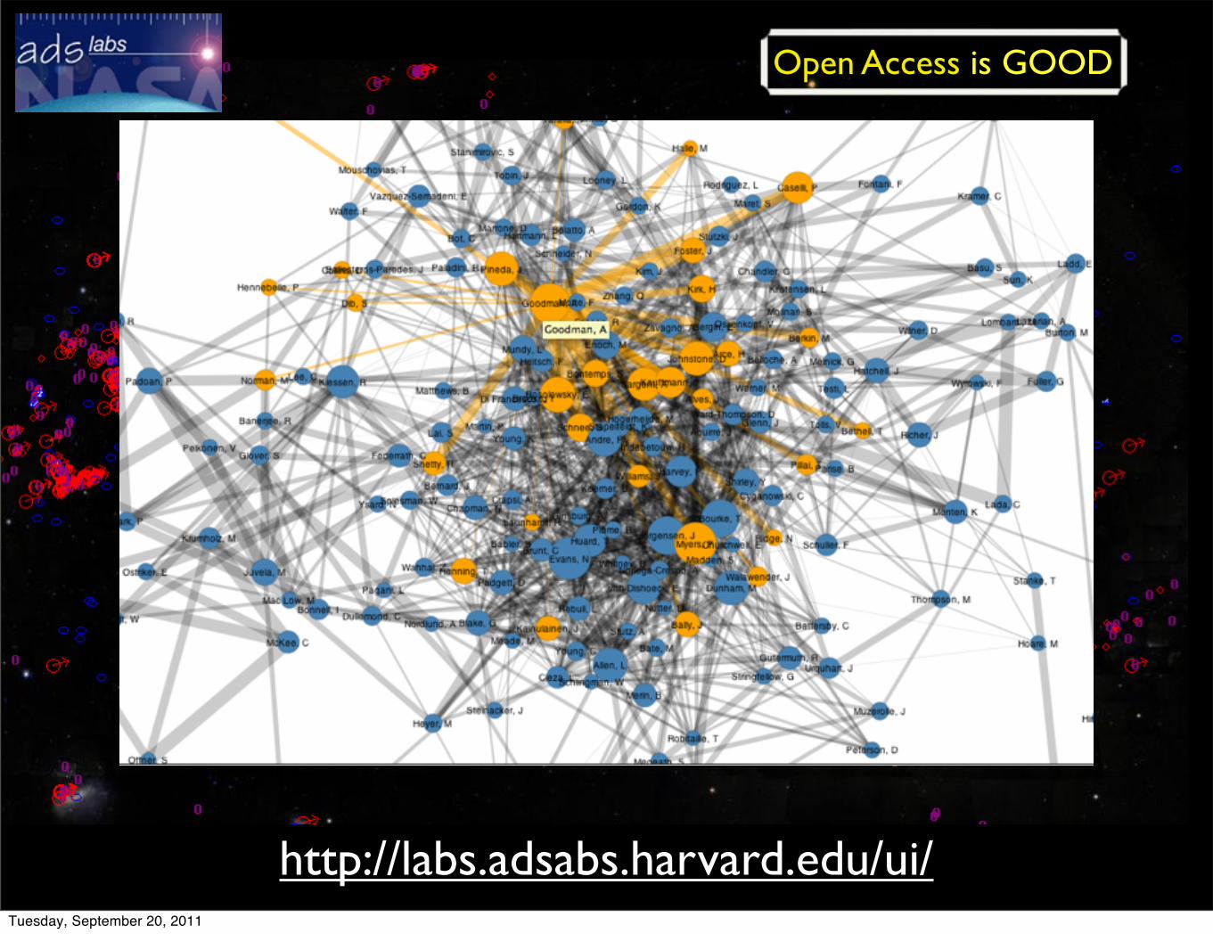
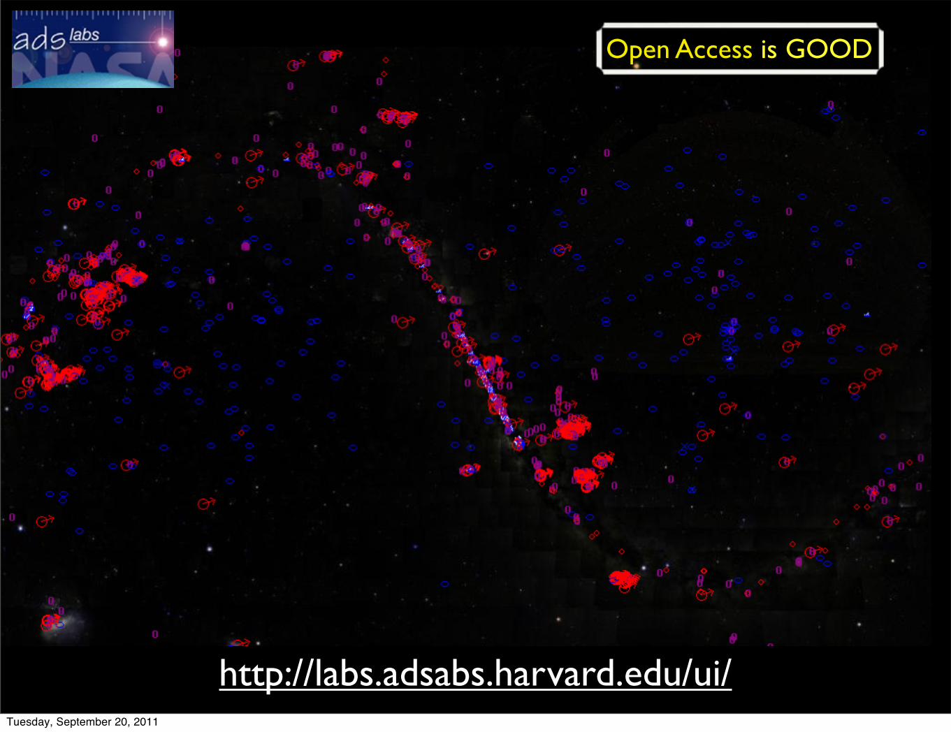
http://labs.adsabs.harvard.edu/ui/
Open Access is GOOD
Tuesday, September 20, 2011
http://labs.adsabs.harvard.edu/ui/
Open Access is GOOD
Tuesday, September 20, 2011
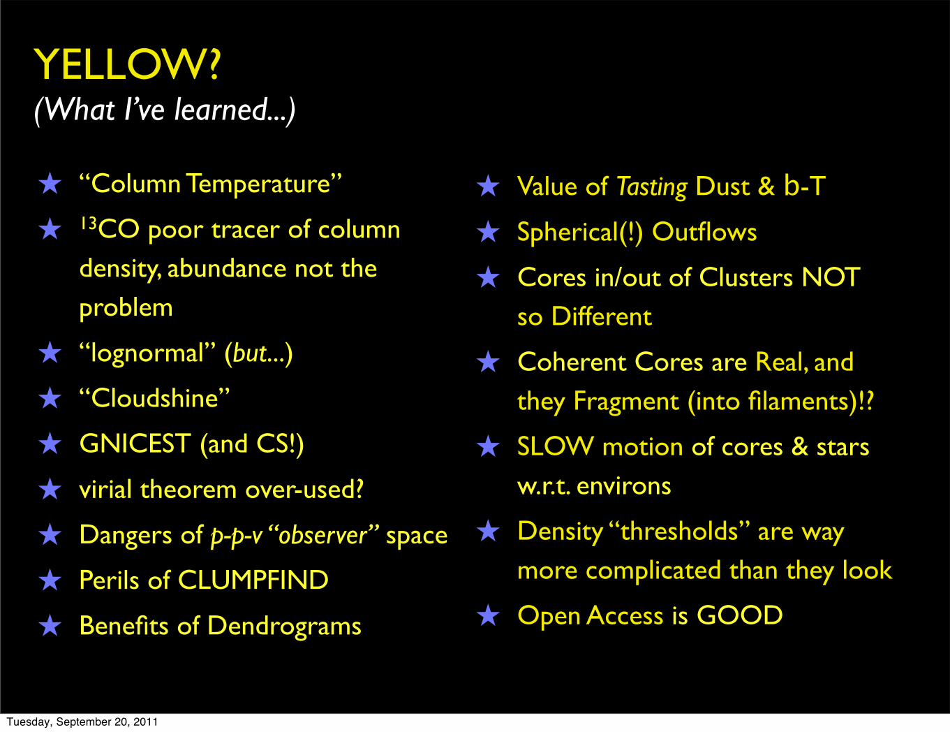
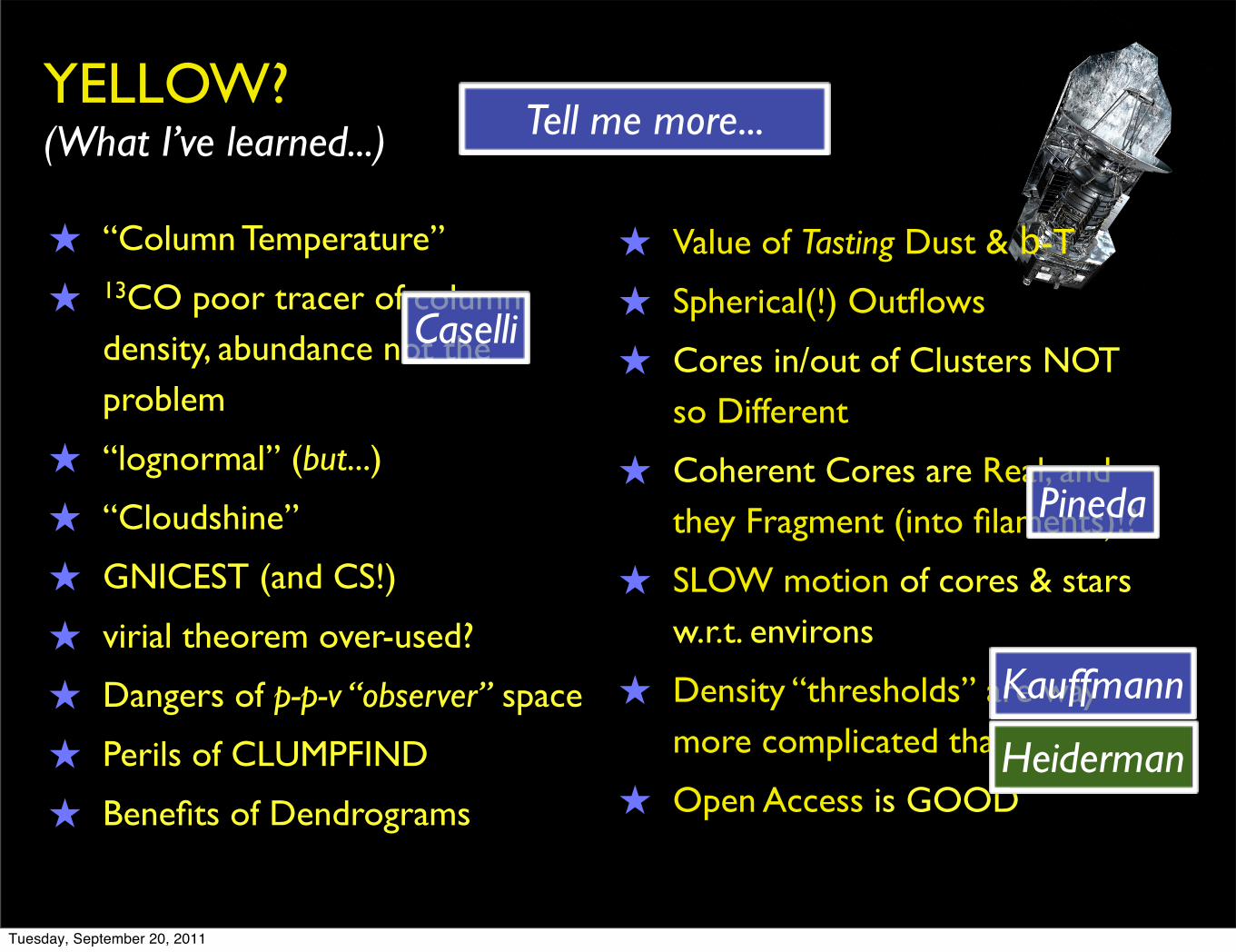
YELLOW?(What I’ve learned...)
★ “Column Temperature”
★ 13CO poor tracer of column density, abundance not the problem
★ “lognormal” (but...)
★ “Cloudshine”
★ GNICEST (and CS!)
★ virial theorem over-used?
★ Dangers of p-p-v “observer” space
★ Perils of CLUMPFIND
★ Benefits of Dendrograms
★ Value of Tasting Dust & b-T
★ Spherical(!) Outflows
★ Cores in/out of Clusters NOT so Different
★ Coherent Cores are Real, and they Fragment (into filaments)!?
★ SLOW motion of cores & stars w.r.t. environs
★ Density “thresholds” are way more complicated than they look
★ Open Access is GOOD
Tuesday, September 20, 2011
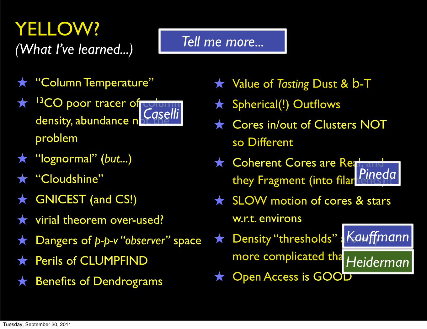
YELLOW?(What I’ve learned...)
★ “Column Temperature”
★ 13CO poor tracer of column density, abundance not the problem
★ “lognormal” (but...)
★ “Cloudshine”
★ GNICEST (and CS!)
★ virial theorem over-used?
★ Dangers of p-p-v “observer” space
★ Perils of CLUMPFIND
★ Benefits of Dendrograms
★ Value of Tasting Dust & b-T
★ Spherical(!) Outflows
★ Cores in/out of Clusters NOT so Different
★ Coherent Cores are Real, and they Fragment (into filaments)!?
★ SLOW motion of cores & stars w.r.t. environs
★ Density “thresholds” are way more complicated than they look
★ Open Access is GOOD
Pineda
Kauffmann
Caselli
Tell me more...
Heiderman
Tuesday, September 20, 2011
What I’m (still) thinking about: B, g, accrete where you are?
Tuesday, September 20, 2011
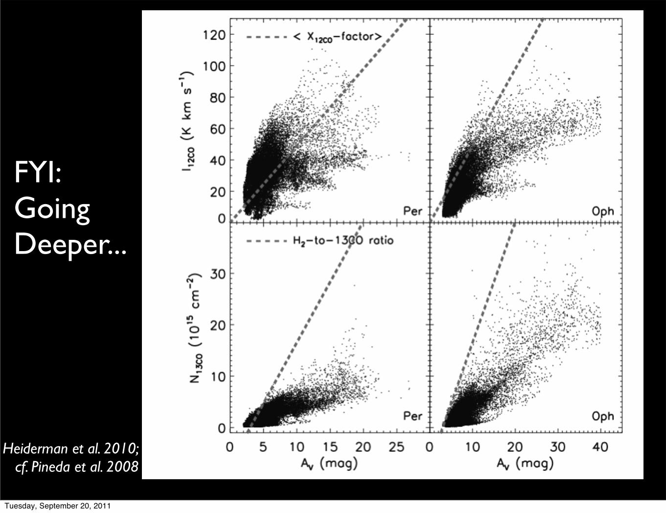
FYI:Going Deeper...
Heiderman et al. 2010,Heiderman et al. 2010; cf. Pineda et al. 2008
Tuesday, September 20, 2011
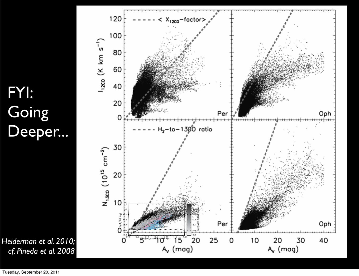
FYI:Going Deeper...
Heiderman et al. 2010,
0.0 0.2 0.4 0.6 0.8 1.0 1.2log(AV(IRAS) (mag))
0.0
0.2
0.4
0.6
0.8
1.0
1.2
log(A V(13 CO
) (mag)
)
0.0
0.2
0.4
0.6
0.8
1.0
1.2
log(Eq
uivalen
t A V(2MAS
S) (ma
g))0.0 0.2 0.4 0.6 0.8 1.0 1.2
log(AV(2MASS) (mag))
0.0
0.2
0.4
0.6
0.8
1.0
1.2
log(A V(IR
AS) (m
ag))
0.0
0.2
0.4
0.6
0.8
1.0
1.2
log(Eq
uivalen
t A V(13 CO) (m
ag))
0.0 0.2 0.4 0.6 0.8 1.0 1.2log(AV(2MASS) (mag))
0.0
0.2
0.4
0.6
0.8
1.0
1.2
log(A V(13 CO
) (mag)
)
0.0
0.2
0.4
0.6
0.8
1.0
1.2
log(Eq
uivalen
t A V(IRAS
) (mag)
)
Heiderman et al. 2010; cf. Pineda et al. 2008
Tuesday, September 20, 2011